FMO6 Web: Polls: https ... · Finite Di erence Methods The Black Scholes PDE Finite di erence...

FMO6 � Web: https://tinyurl.com/ycaloqk6 Polls: https://pollev.com/johnarmstron561

FMO6 � Web:

https://tinyurl.com/ycaloqk6 Polls:

https://pollev.com/johnarmstron561

Lecture 8

Dr John Armstrong

King's College London

July 22, 2019

https://tinyurl.com/ycaloqk6





Finite Di�erence Methods






Risk neutral pricing

We have learned how to price the following by Monte Carlo

European Call Options

European Put Options

Digital Call Options

Knockout Options

Asian Options

But what options can't we price?





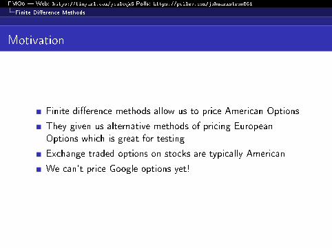
Motivation

Finite di�erence methods allow us to price American Options

They given us alternative methods of pricing EuropeanOptions which is great for testing

Exchange traded options on stocks are typically American

We can't price Google options yet!





European Options

In your project you might want to numerically test examples aboutEuropean options. It helps to know that:

Exchange traded options on indices are typically European

Call options on non dividend paying stocks have the sameprice whether they are European or American.

So if you want to �nd real data to test a theory, you can.





The Black�Scholes PDE

Finite di�erence methods

Finite di�erence methods are a method of solving PDEs(partial di�erential equations)

In a Black�Scholes world, the risk neutral price of a derivativeon a stock obeys the Black�Scholes PDE.

Vt +1

2σ2S2VSS + rSVS − rV = 0

∂V

∂t+

1

2σ2S2∂

2V

∂S2+ rS

∂V

∂S− rV = 0

V is the price of the derivative. S is the stock price. t is time.






How to remember the PDE

It's a PDE for V

It's �rst order in time

It's second order in S

It's linear

In other words it looks like this:

∗∂V∂t

+ ∗∂2V

∂S2+ ∗∂V

∂S+ ∗V = 0






Dimensional analysis: The S terms

To remember the coe�cients

WLOG the coe�cient of

∂V

∂t= 1

Each term has units of

$years−1

So the equation must be

∂V

∂t+ ∗S2∂

2V

∂S2+ ∗S ∂V

∂S+ ∗V = 0

with the ∗'s having units of years−1






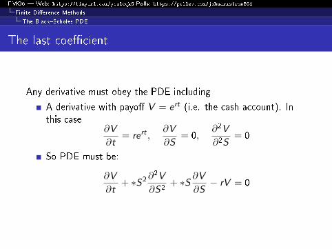
The last coe�cient

Any derivative must obey the PDE including

A derivative with payo� V = ert (i.e. the cash account). Inthis case

∂V

∂t= rert ,

∂V

∂S= 0,

∂2V

∂2S= 0

So PDE must be:

∂V

∂t+ ∗S2∂

2V

∂S2+ ∗S ∂V

∂S− rV = 0






The second to last coe�cient

The stock also obeys the PDE. It satis�es

∂V

∂t= 0,

∂V

∂S= 1,

∂2V

∂2S= 0

We deduce that the PDE must be:

∂V

∂t+ ∗S2∂

2V

∂S2+ rS

∂V

∂S− rV = 0






Conclusion

All you have to remember is that ∗ = 12σ2!

∂V

∂t+

1

2σ2S2∂

2V

∂S2+ rS

∂V

∂S− rV = 0

Note that the units are dollars/year throughout.





The Explicit Method

The Explicit Method

Suppose that I know the payo� at time T as a function of S .This is VT (S).

I can then compute ∂V∂S and ∂2V

∂S2.

Plugging this into the Black�Scholes PDE I can now compute

∂V

∂t

Using

VT−δt ≈ Vt −∂V

∂tδt

we can now compute VT−δt

So given payo� function at time T we can approximate theprice at VT−δt .

Stepping back in time we can compute the price at time 0.





The Explicit Method

Picture of algorithm





The Explicit Method

Grid notation

Equivalently we compute a grid of values showing how price Vvaries with S and t.

δS =Smax

M, δt =

T

N





The Explicit Method

Let V(i ,j) be the value at point (i , j) in this grid with i and jintegers.

We have central di�erence estimate

∂V

∂S (i ,j)≈

V(i ,j+1) − V(i ,j−1)

2δS

Second derivative estimate

∂2V

∂S2 (i ,j)≈

V(i ,j+1) − 2V(i ,j) + V(i ,j−1)

(δS)2

By PDE, plus backwards estimate for ∂V∂t :

V(i−1,j) ≈ V(i ,j) − δt∂V

∂t (i ,j)

≈ V(i ,j) + δt

(1

2σ2S2VSS + rSVS − rV

)





The Explicit Method

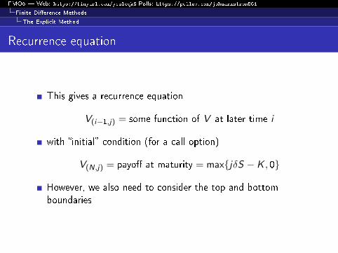
Recurrence equation

This gives a recurrence equation

V(i−1,j) = some function of V at later time i

with �initial� condition (for a call option)

V(N,j) = payo� at maturity = max{jδS − K , 0}

However, we also need to consider the top and bottomboundaries





The Explicit Method

Boundary conditions





The Explicit Method

Boundary conditions for European Call Option

Our recurrence equation breaks down at the top and bottomboundaryWe impose boundary conditions derived using simple heuristicarguments (or more rigorously limiting arguments)When S = 0, a call option is worthless. So V (t, 0) = 0. SoV(i ,0) = 0.When S = Smax, it is unlikely to end out of the money. So it isworth roughly the same as a portfolio consisting of one unit ofstock and −K zero coupon bonds. HenceV (t, Smax) ≈ Smax − e−r(T−t)K . In detail:

V (t,Smax) = e−r(T−t)EQ(payo�|St = Smax)

≈ e−r(T−t)EQ(ST − K |St = Smax)

= EQ(e−r(T−t)ST |St = Smax)− e−r(T−t)EQ(K |St = Smax)

= Smax − e−r(T−t)K





The Explicit Method

Choosing boundary conditions

We do not know the exact price along the top and bottomboundary, we must use approximation arguments.

If the boundary is far enough away, our solution won't be verysensitive to the boundary.

What is far enough away? You need to choose Smax so thatour approximation on the top boundary is reasonably accurate.Recall that over a time interval δt the change in the log stockprice is normally distributed with mean (r − 1

2σ2)δt and

standard deviation σ√t. So you might choose

Smax = e−(r−12σ2)T+4σ

√TK as a 4 standard deviation

movement in the log of the stock price is fairly unlikely.





The Explicit Method

Boundary conditions for European Call Option

So our boundary conditions are:

V(N,j) = max{Sj − K , 0}

V(i ,0) = 0

V(i ,M) = Smax − e−r(T−t)K

We have a recurrence relation for all other V(i ,j)

We can now solve this in Matlab





The Explicit Method

Boundary conditions





The Explicit Method

Step 1





The Explicit Method

Step 2





The Explicit Method

Step 3





The Explicit Method

Explicit calculation

Before proceeding to the Matlab, let's compute the di�erenceequation explicitly.

Black�Scholes PDE

∂V

∂t+

1

2σ2S2∂

2V

∂S2+ rS

∂V

∂S− rV = 0

Finite di�erence equations

V(i ,j) − V(i−1,j)

∂t+

1

2σ2S2

j

(V(i ,j+1) − 2V(i ,j) + V(i ,j−1)

(δS)2

)+ rSj

(V(i ,j+1) − V(i ,j−1)

2δS

)− rV(i ,j) = 0

Central di�erence in S . Backwards di�erence in t.





The Explicit Method

Rearrange to get

V(i−1,j) = αjV(i ,j+1) + βjV(i ,j) + γjV(i ,j−1)

where

α =1

2

σ2S2j δt

δS2+

rSj2δS

δt

β = 1−σ2S2

j δt

δS2− rδt

γ =1

2

σ2S2j δt

δS2−

rSj2δS

δt

Check: everything is dimensionless.





The Explicit Method

Matlab code - slide 1

function [ price, V ] = priceCallByExplicitMethod( ...

K, T, S0, r, sigma, SMax, N, M )

%PRICECALLBYEXPLICITMETHOD Price a call option by the explicit method

% using the Black Scholes PDE directly

iMin = 1;

iMax = N+1;

jMin = 1;

jMax = M+1;

dS = SMax/M;

dt = T/N;

t=0:dt:T;

S=0:dS:SMax;





The Explicit Method

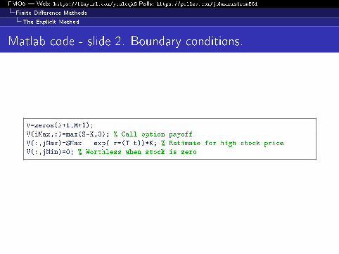
Matlab code - slide 2. Boundary conditions.

V=zeros(N+1,M+1);

V(iMax,:)=max(S-K,0); % Call option payoff

V(:,jMax)=SMax - exp(-r*(T-t))*K; % Estimate for high stock price

V(:,jMin)=0; % Worthless when stock is zero





The Explicit Method

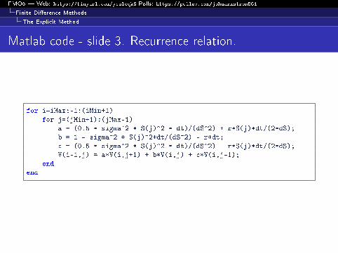
Matlab code - slide 3. Recurrence relation.

for i=iMax:-1:(iMin+1)

for j=(jMin+1):(jMax-1)

a = (0.5 * sigma^2 * S(j)^2 * dt)/(dS^2) + r*S(j)*dt/(2*dS);

b = 1 - sigma^2 * S(j)^2*dt/(dS^2) - r*dt;

c = (0.5 * sigma^2 * S(j)^2 * dt)/(dS^2) - r*S(j)*dt/(2*dS);

V(i-1,j) = a*V(i,j+1) + b*V(i,j) + c*V(i,j-1);

end

end





The Explicit Method

Final touches

% We want to extract the actual price at S0, so use

% polynomial interpolation since S0 may not fall on a grid point

s0Index = S0/dS+jMin;

price = linearInterpolate(V(iMin,:),s0Index);

end





The Explicit Method

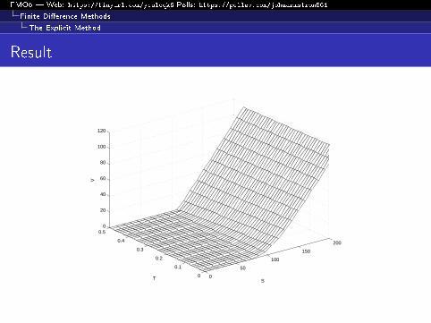
Result

0

50

100

150

200

0

0.1

0.2

0.3

0.4

0.50

20

40

60

80

100

120

ST

V





The Explicit Method

Numerical Results

Parameter choices

σ = 0.3

S0 = 108

T = 0.5

K = 110

r = 0.05

Taking Smax = e−(r−12σ2)T+4σ

√T

Black�Scholes Price 9.455

Finite di�erence with M = 100, N = 500, 9.454

Finite di�erence with M = 150, N = 500, 8.7× 10148

Something has gone terribly wrong. This is called instability.




The Heat Equation

The Heat Equation




The Heat Equation

Heat Equation - Motivation

The Black�Scholes PDE is so complex because we've made apoor choice of variables.

Clearly life would be easier if eliminated r from the equations.We can do this by working in real terms

W = e−rtV

S = e−rtS

We also know that by working with x = log S instead of Severything should be easier mathematically.

W = e−rtV , x = −rt + log(S)

In fact we can make things even easier by taking:

W = e−rtV , x = −(r − 1

2σ2)t + log(S)

because x then follows driftless Brownian motion




The Heat Equation

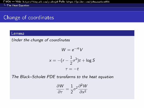
Change of coordinates

Lemma

Under the change of coordinates

W = e−rtV

x = −(r − 1

2σ2)t + log S

τ = −t

The Black�Scholes PDE transforms to the heat equation

∂W

∂τ=

1

2σ2∂2W

∂x2




The Heat Equation

Proof - step 1

The Black�Scholes PDE is

∂V

∂t+

1

2σ2S2∂

2V

∂S2+ rS

∂V

∂S− rV = 0

Writing V = ertW we get:

ert∂W

∂t+ rertW +

1

2σ2S2ert

∂2W

∂S2+ rSert

∂W

∂S− rertW = 0

Cancelling the ert terms:

∂W

∂t+

1

2σ2S2∂

2W

∂S2+ rS

∂W

∂S= 0 (1)




The Heat Equation

Proof - step 2

∂W

∂t=∂W

∂τ

∂τ

∂t+∂W

∂x

∂x

∂t= −∂W

∂τ−(r − 1

2σ2)∂W

∂x

Note there is a potential trap here because partial di�erentiationnotation is not that great. It would be better to write

∂W

∂t=:

∂1W

∂0S∂1t

to emphasize that we are holding S �xed. And to write

∂W

∂τ=:

∂1W

∂0x∂1τ

to emphasize that we are now holding x �xed.So even though τ = −t

∂W

∂t6= −∂W

∂τ




The Heat Equation

Proof - step 2, continued

∂W

∂t=∂W

∂τ

∂τ

∂t+∂W

∂x

∂x

∂t= −∂W

∂τ−(r − 1

2σ2)∂W

∂x

∂W

∂S=∂W

∂τ

∂τ

∂S+∂W

∂x

∂x

∂S=

1

S

∂W

∂x

∂2W

∂S2= − 1

S2

∂W

∂x+

1

S

∂

∂S

(∂W

∂x

)= − 1

S2

∂W

∂x+

1

S2

∂2W

∂x2

So equation (1) two slides ago becomes:

−∂W∂τ−(r − 1

2σ2)∂W

∂x+

1

2σ2∂2W

∂x2− 1

2σ2∂W

∂x+ r

∂W

∂x= 0

which simpli�es to:∂W

∂τ=

1

2σ2∂2W

∂x2




The Heat Equation

What have we gained?

The advantages of the heat equation are:

The Heat equation has constant coe�cients which makes itmuch easier to understand. This is the main purpose of thechange.

There is a huge literature on the heat equation which we canexploit

The coordinates are �better� because they scale correctly. Forlarger stock values, we should use larger grid sizes. A onedollar step size is a large step size for a one dollar stock, but asmall step size for a one hundred dollar stock. Taking logsautomatically scales things.

Against this:

The boundary conditions are a little more awkward

For pricing barrier options, we have transformed constantbarriers (easy) to curved barriers (harder)




The Heat Equation

Slightly di�erent coordinates

Lemma

Under the change of coordinates

W = e−rtV

x = −(r − 1

2σ2)t + log S

The Black�Scholes PDE transforms to the time reversed heat

equation∂W

∂t= −1

2σ2∂2W

∂x2




The Heat Equation

Hazard Warning

If you try to prove this directly you will almost certainly make themistake of thinking

∂1W

∂0S∂1t=

∂1W

∂0x∂1t

because in the ambiguous conventional notation this becomes

∂W

∂t=∂W

∂t

which looks plausible, but isn't always true!




The Heat Equation

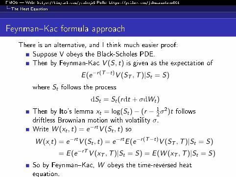
Feynman�Kac formula approach

There is an alternative, and I think much easier proof:

Suppose V obeys the Black-Scholes PDE.Then by Feynman-Kac V (S , t) is given as the expectation of

E (e−r(T−t)V (ST ,T )|St = S)

where St follows the process

dSt = St(rdt + σdWt)

Then by Ito's lemma xt = log(St)− (r − 12σ2)t follows

driftless Brownian motion with volatility σ.Write W (xt , t) = e−rtV (St , t) so

W (x,t) = e−rtV (St , t) = e−rtE (e−r(T−t)V (ST ,T )|St = S)

= E (e−rTV (xT ,T )|St = S) = E (W (xT ,T )|St = S)

So by Feynman�Kac, W obeys the time-reversed heatequation.




The Heat Equation

Feynman-Kac

The solution to the PDE

∂u

∂t+ µ(x , t)

∂u

∂x+

1

2σ2(x , t)

∂2u

∂x2− r(x , t)u(x , t) = 0

with �nal condition u(x ,T ) = ψ(T ) is given by

E(e−

∫ Tt r(Xτ ,τ)ψ(XT )|Xt = x

)where X follows the process:

dXt = µ(Xt , t)dt + σ(Xt , t)dWt

for Wt a Brownian motion.




The Heat Equation

Boundary conditions in new coordinates

Old boundary conditions for call option

V (t, S) ≈ 0 for small S

V (t, S) ≈ S − e−r(T−t)K for large S

V (T ,S) = max{S − K , 0}

W = e−rtV , S = e(r−12σ2)t+x

Boundary conditions for call option

W (t, xmin) ≈ 0

W (t, xmax) ≈ e−12σ2t+xmax − e−rTK

W (T , x) = max{e−12σ2T+x − e−rTK , 0}




The Heat Equation

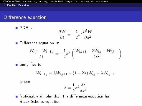
Di�erence equation

PDE is∂W

∂t= −1

2σ2∂2W

∂x2

Di�erence equation is:

Wi ,j −Wi−1,jδt

= −12σ2(Wi ,j+1 − 2Wi ,j +Wi ,j−1

δx2

)Simpli�es to:

Wi−1,j = λWi ,j+1 + (1− 2λ)Wi ,j + λWi ,j−1

where

λ =1

2σ2

δt

δx2

Noticeably simpler than the di�erence equation forBlack-Scholes equation




The Heat Equation

Observation

Equation is


This is a weighted average of Wi ,j+1, (1− 2λ)Wi ,j andλWi ,j−1 so long as (1− 2λ) > 0.

Physically temperature after a small time is a weightedaverage of nearby temperatures.




The Heat Equation

Financially

In terms of x

Each time period δt, x moves up δx with Q-probability λx moves down with Q-probability λx stays the same with probability 1− 2λ

or in terms of S

Stock moves up by a factor e(r−12σ2)δt+δx with Q-probability λ

Moves up by a factor e(r−12σ2)δt with Q-probability 1− 2λ

Moves down by a factor e(r−12σ2)δt−δx with Q-probability λ

Prices are discounted risk neutral expectations




The Heat Equation

Con�rmation of the interpretation

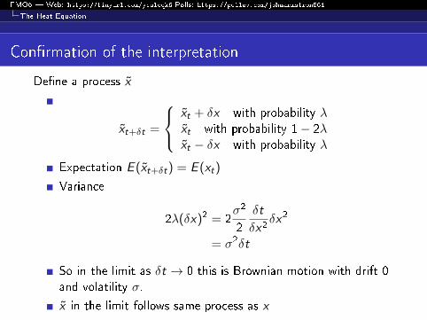
De�ne a process x

xt+δt =

xt + δx with probability λxt with probability 1− 2λxt − δx with probability λ

Expectation E (xt+δt) = E (xt)

Variance

2λ(δx)2 = 2σ2

2

δt

δx2δx2

= σ2δt

So in the limit as δt → 0 this is Brownian motion with drift 0and volatility σ.

x in the limit follows same process as x




The Heat Equation

Points used

Not all the points on the boundary are used in the calculation.White circles represent data that is not needed to calculate price atblack points.




The Heat Equation

Trinomial Tree

Pricing using a trinomial tree with risk neutral probabilities λ,1− 2λ, λ is equivalent to a heat equation method.

Easier to program because there is no need for boundaryconditions at top and bottom. This is at the expense ofunnecessary computations at unlikely points.




The Heat Equation

Non-convergence

Note that if you keepδx

δtas a constant c as you re�ne the grid, all data used comesfrom a �xed triangle

Therefore the trinomial tree method cannot possibly convergeas δt tends to 0 with c �xed. This is because you need toconsider payo�s at T outside the triangle to compute theexpectation correctly.




Stability

Stability




Stability

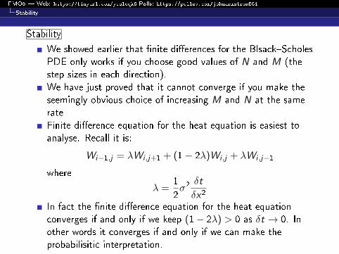
Stability

We showed earlier that �nite di�erences for the Blsack�ScholesPDE only works if you choose good values of N and M (thestep sizes in each direction).We have just proved that it cannot converge if you make theseemingly obvious choice of increasing M and N at the samerateFinite di�erence equation for the heat equation is easiest toanalyse. Recall it is:


where

λ =1

2σ2

δt

δx2

In fact the �nite di�erence equation for the heat equationconverges if and only if we keep (1− 2λ) > 0 as δt → 0. Inother words it converges if and only if we can make theprobabilisitic interpretation.




Stability

Theorem

If we choose a �xed value for

λ =1

2σ2

δt

δx2

with 1− 2λ > 0 and consider the sequence of approximate

solutions given by letting δx → 0 in the explicit scheme for the heat

equation. This will converge to a solution of the heat equation with

the desired boundary conditions (we should add that we need some

conditions such as that the boundary is compact and the boundary

conditions are continuous).




Stability

Components of proof

The proof is beyond the scope of this course.Prove the problem is well-posed, i.e. there is a unique solutiondepending continuously on the boundary conditions.Prove the scheme is consistent, i.e. the approximate operatorsused in the scheme are close to the operators in the PDE.Prove the scheme is stable, i.e. if you start with a small valuesW at the �nal time, they will remain small as you move backin time. This means that if your solution is fairly accurate buthas a small rounding ε then the e�ects of that rounding errorwill remain small as you move back in time. (Note that theequation is linear, so to compute the e�ects of the roundingerror on the scheme we can simply apply the scheme to therounding error.)Apply the Lax Equivalence Theorem that says that for wellposed problems, stability is equivalent to convergence.

Note that since our process takes weighted averages it will benumerically stable as the average of small things is still small.




Stability

Remarks

Instability shows itself numerically as extreme sensitivity torounding errors - i.e. numerical instability.

Our example of a calculation with bad choices of M and Nillustrates the instability of the scheme vividly.




Stability

Rate of Convergence

For given boundary conditions, the Explicit �nite di�erencescheme for the heat equation using �xed

λ =1

2σ2

δt

δx2

with 1− 2λ > 0 has an error of O(δt).




Heat equation implementation

Implementation

Parameters

K , T , S0, r , σ, N, M, nSds.

N = number of time steps

M = number of x steps

nSds = number of standard deviations to include each side ofx0 in the grid. 8 standard deviations would be plenty.





Initialization Code

x0 = log( S0 );

xMin = x0 - nSds*sqrt(T)*sigma;

xMax = x0 + nSds*sqrt(T)*sigma;

dt = T/N;

dx = (xMax-xMin)/M;

iMin = 1;

iMax = N+1;

jMin = 1;

jMax = M+1;

x = xMin:dx:xMax;

t = 0:dt:T;

lambda = 0.5*sigma^2 * dt/(dx)^2;





Looping Code

% Use boundary condition to create vector currW

currW=max(exp(-0.5*sigma^2*T + x) - exp(-(r*T))*K,0);

for i=iMax:-1:iMin+1

% Use recurrence for all points except jMin and jMax

currW(jMin+1:jMax-1)= lambda*currW((jMin):(jMax-2)) ...

+(1-2*lambda)*currW((jMin+1):(jMax-1)) ...

+ lambda*currW((jMin+2):(jMax));

% Use boundary conditions for jMin and jMax

currW(jMin)=0;

currW(jMax)=exp(-0.5*sigma^2 * t(i) + x(jMax))- exp(-r*T)*K;

end

price = currW(iMin,jMin+M/2);





Remarks

The code is written less naively

We use a single vector currW which holds the option price atthe current time.

This saves a lot of memory

We have no loop across the space dimension. This code isvectorized.

This makes it much faster.





Convergence

10−5

10−4

10−3

10−2

10−1

100

10−4

10−3

10−2

10−1

100

101

dt

erro

r

Convergence of explicit method

Figure: Convergence of the explicit method (error against δt)





Remarks

Plot shows convergence to the Black�Scholes price withnSds=8.

It has rate of convergence predicted by theory

(Note theory says it will converge to solution with ourapproximate boundary conditions rather than the true solution.Our boundary condition approximation is very accurate whennSds=8)





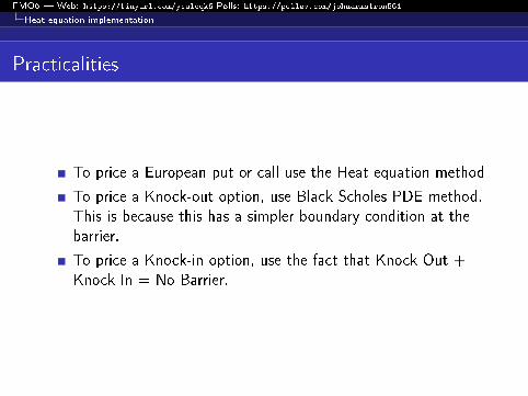
Practicalities

To price a European put or call use the Heat equation method

To price a Knock-out option, use Black Scholes PDE method.This is because this has a simpler boundary condition at thebarrier.

To price a Knock-in option, use the fact that Knock Out +Knock In = No Barrier.





American Options

For an American option, suppose we've computed the priceVi ,j at time point i .

Suppose we compute Vi−1,j by using the di�erence equationfor the Black�Scholes PDE

This is the price at time i − 1 of an option you can onlyexercise from time i onwards.

Let Ei ,j be the value obtained by exercising at time i

Vi−1,j = max{Vi−1,j ,Ei−1,j}





More explicitly

We haveVi−1,j = αjVi ,j+1 + βjVi ,j + γjVi ,j−1

where αj , βj and γj are as before.

Ei ,j = (Sj − K )+

Vi−1,j = max{Vi ,j ,Ei ,j}.

The same technique works for the heat equation and trinomial treeapproaches.



FMO6 Web: Polls: https ... · Finite Di erence Methods The Black Scholes PDE Finite di erence...

Documents

Transcript of FMO6 Web: Polls: https ... · Finite Di erence Methods The Black Scholes PDE Finite di erence...