Structural Engineering III.pdf
61
1 Joint Displacements and Forces 1. Coordinate Systems y z x x z y Fig. 1: Coordinate System1 Fig. 2: Coordinate System2 (widely used and also applied in this course) (used in some formulations) 2. Sign Convention for Joint Displacements and Forces u y F y y M y u x F x x M x z M z u z F z Fig. 3: Sign convention for Displacements Fig. 4: Sign convention for Forces 3. Sign Convention for Two-dimensional Problems u y F y z u x M z F x Fig. 5: Two-Dimensional Displacements Fig. 6: Two-Dimensional Forces
Transcript of Structural Engineering III.pdf
1
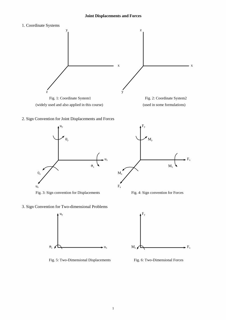
Joint Displacements and Forces
1. Coordinate Systems y z
x x
z y
Fig. 1: Coordinate System1 Fig. 2: Coordinate System2
(widely used and also applied in this course) (used in some formulations)
2. Sign Convention for Joint Displacements and Forces
uy Fy
y My
ux Fx
x Mx
z Mz
uz Fz
Fig. 3: Sign convention for Displacements Fig. 4: Sign convention for Forces
3. Sign Convention for Two-dimensional Problems
uy Fy
z ux Mz Fx
Fig. 5: Two-Dimensional Displacements Fig. 6: Two-Dimensional Forces
2
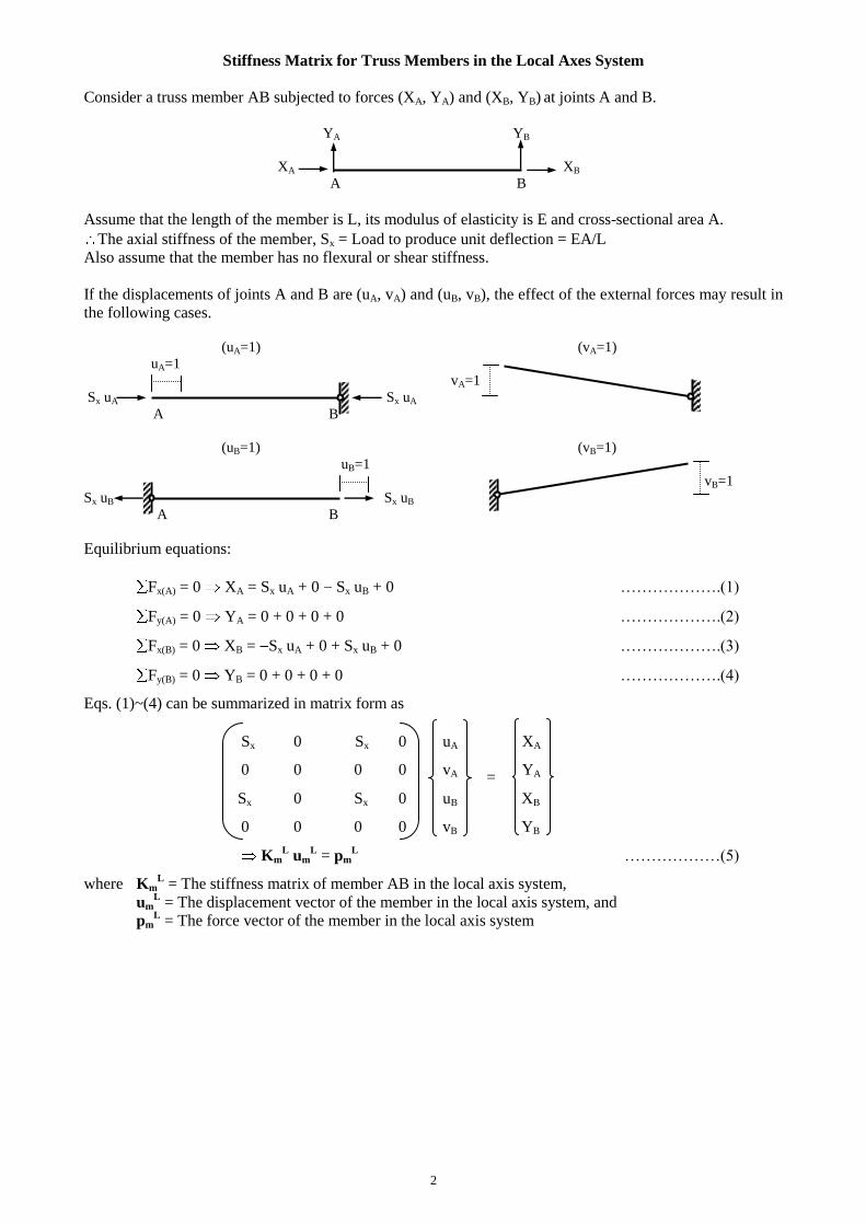
Stiffness Matrix for Truss Members in the Local Axes System
Consider a truss member AB subjected to forces (XA, YA) and (XB, YB) at joints A and B.
YA YB
XA XB A B
Assume that the length of the member is L, its modulus of elasticity is E and cross-sectional area A.
The axial stiffness of the member, Sx = Load to produce unit deflection = EA/L
Also assume that the member has no flexural or shear stiffness.
If the displacements of joints A and B are (uA, vA) and (uB, vB), the effect of the external forces may result in
the following cases.
(uA=1) (vA=1)
uA=1
vA=1
Sx uA Sx uA
A B
(uB=1) (vB=1)
uB=1
vB=1
Sx uB Sx uB
A B
Equilibrium equations:
Fx(A) = 0 XA = Sx uA + 0 Sx uB + 0 ……………….(1)
Fy(A) = 0 YA = 0 + 0 + 0 + 0 ……………….(2)
Fx(B) = 0 XB = Sx uA + 0 + Sx uB + 0 ……………….(3)
Fy(B) = 0 YB = 0 + 0 + 0 + 0 ……………….(4)
Eqs. (1)~(4) can be summarized in matrix form as
Sx 0 Sx 0 uA XA
0 0 0 0 vA YA
Sx 0 Sx 0 uB XB
0 0 0 0 vB YB
KmL um
L = pm
L ………………(5)
where KmL = The stiffness matrix of member AB in the local axis system,
umL = The displacement vector of the member in the local axis system, and
pmL = The force vector of the member in the local axis system
=
3
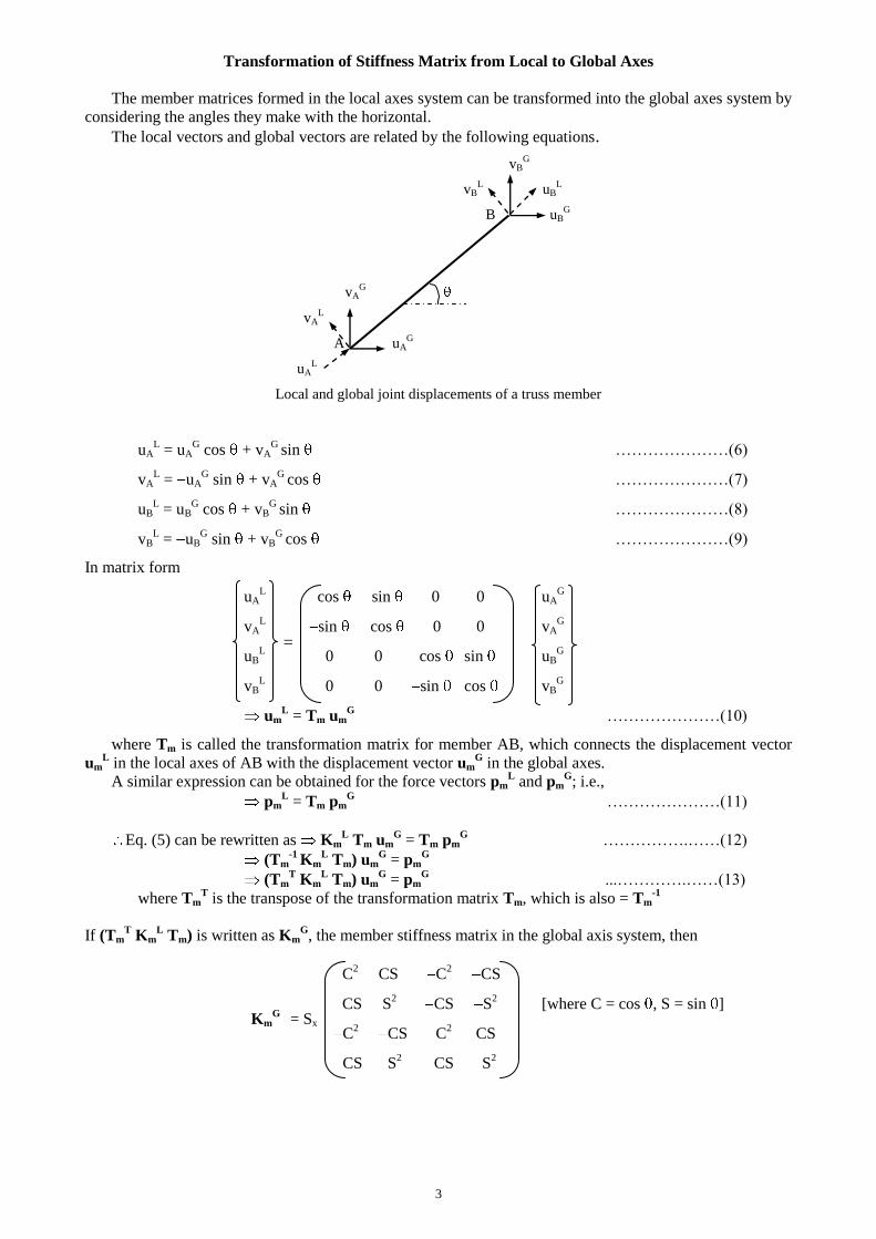
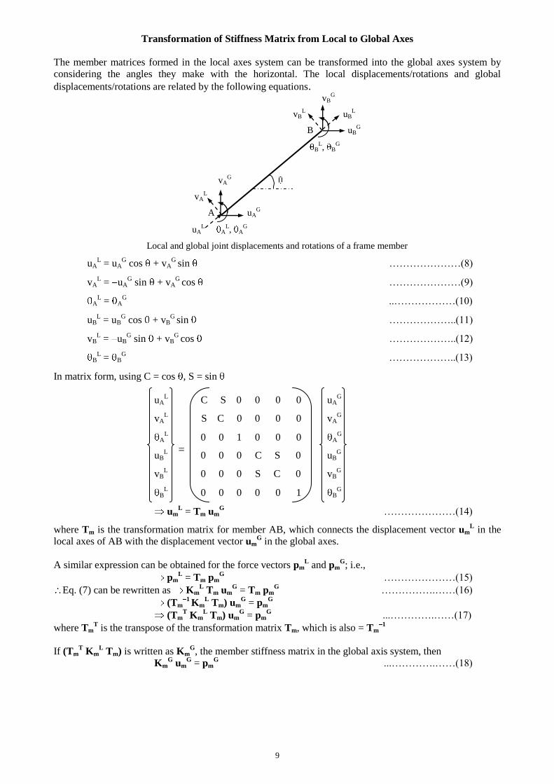
Transformation of Stiffness Matrix from Local to Global Axes
The member matrices formed in the local axes system can be transformed into the global axes system by
considering the angles they make with the horizontal.
The local vectors and global vectors are related by the following equations.
vBG
vBL uB
L
B uBG
vAG
vAL
A uAG
uAL
Local and global joint displacements of a truss member
uAL = uA
G cos + vA
G sin …………………(6)
vAL = uA
G sin + vA
G cos …………………(7)
uBL = uB
G cos + vB
G sin …………………(8)
vBL = uB
G sin + vB
G cos …………………(9)
In matrix form
uAL cos sin 0 0 uA
G
vAL sin cos 0 0 vA
G
uBL 0 0 cos sin uB
G
vBL 0 0 sin cos vB
G
umL = Tm um
G …………………(10)
where Tm is called the transformation matrix for member AB, which connects the displacement vector
umL in the local axes of AB with the displacement vector um
G in the global axes.
A similar expression can be obtained for the force vectors pmL and pm
G; i.e.,
pmL = Tm pm
G …………………(11)
Eq. (5) can be rewritten as KmL Tm um
G = Tm pm
G …………….……(12)
(Tm-1
KmL Tm) um
G = pm
G
(TmT Km
L Tm) um
G = pm
G ...………….……(13)
where TmT is the transpose of the transformation matrix Tm, which is also = Tm
-1
If (TmT Km
L Tm) is written as Km
G, the member stiffness matrix in the global axis system, then
C2 CS C
2 CS
CS S2 CS S
2 [where C = cos , S = sin ]
C2 CS C
2 CS
CS S2 CS S
2
=
= Sx KmG
4
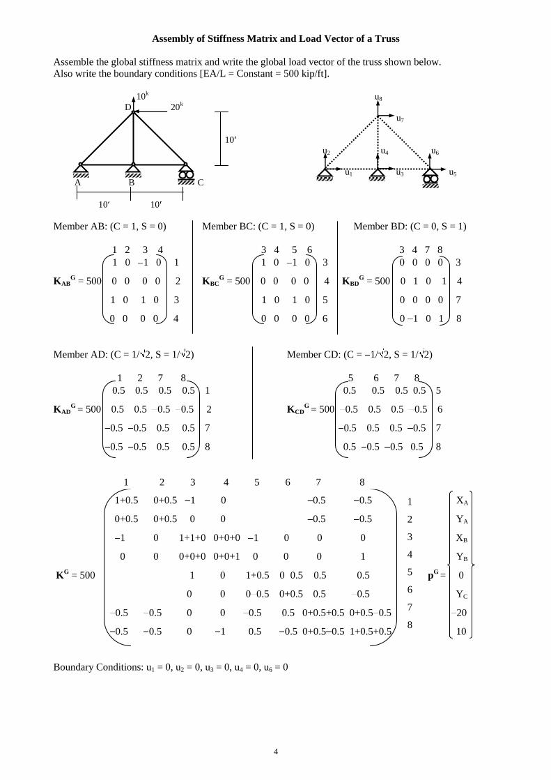
Assembly of Stiffness Matrix and Load Vector of a Truss
Assemble the global stiffness matrix and write the global load vector of the truss shown below.
Also write the boundary conditions [EA/L = Constant = 500 kip/ft].
10
k u8
D 20k
u7
10
u2 u4 u6
u1 u3 u5
A B C
10 10
Member AB: (C = 1, S = 0) Member BC: (C = 1, S = 0) Member BD: (C = 0, S = 1)
1 2 3 4 3 4 5 6 3 4 7 8
1 0 1 0 1 1 0 1 0 3 0 0 0 0 3
KABG = 500 0 0 0 0 2 KBC
G = 500 0 0 0 0 4 KBD
G = 500 0 1 0 1 4
1 0 1 0 3 1 0 1 0 5 0 0 0 0 7
0 0 0 0 4 0 0 0 0 6 0 1 0 1 8
Member AD: (C = 1/ 2, S = 1/ 2) Member CD: (C = 1/ 2, S = 1/ 2)
1 2 7 8 5 6 7 8
0.5 0.5 0.5 0.5 1 0.5 0.5 0.5 0.5 5
KADG
= 500 0.5 0.5 0.5 0.5 2 KCDG
= 500 0.5 0.5 0.5 0.5 6
0.5 0.5 0.5 0.5 7 0.5 0.5 0.5 0.5 7
0.5 0.5 0.5 0.5 8 0.5 0.5 0.5 0.5 8
1+0.5 0+0.5 1 0 0.5 0.5 XA
0+0.5 0+0.5 0 0 0.5 0.5 YA
1 0 1+1+0 0+0+0 1 0 0 0 XB
0 0 0+0+0 0+0+1 0 0 0 1 YB
KG = 500 1 0 1+0.5 0 0.5 0.5 0.5 p
G = 0
0 0 0 0.5 0+0.5 0.5 0.5 YC
0.5 0.5 0 0 0.5 0.5 0+0.5+0.5 0+0.5 0.5 20
0.5 0.5 0 1 0.5 0.5 0+0.5 0.5 1+0.5+0.5 10
Boundary Conditions: u1 = 0, u2 = 0, u3 = 0, u4 = 0, u6 = 0
1 2 3 4 5 6 7 8
1
2
3
4
5
6
7
8
5
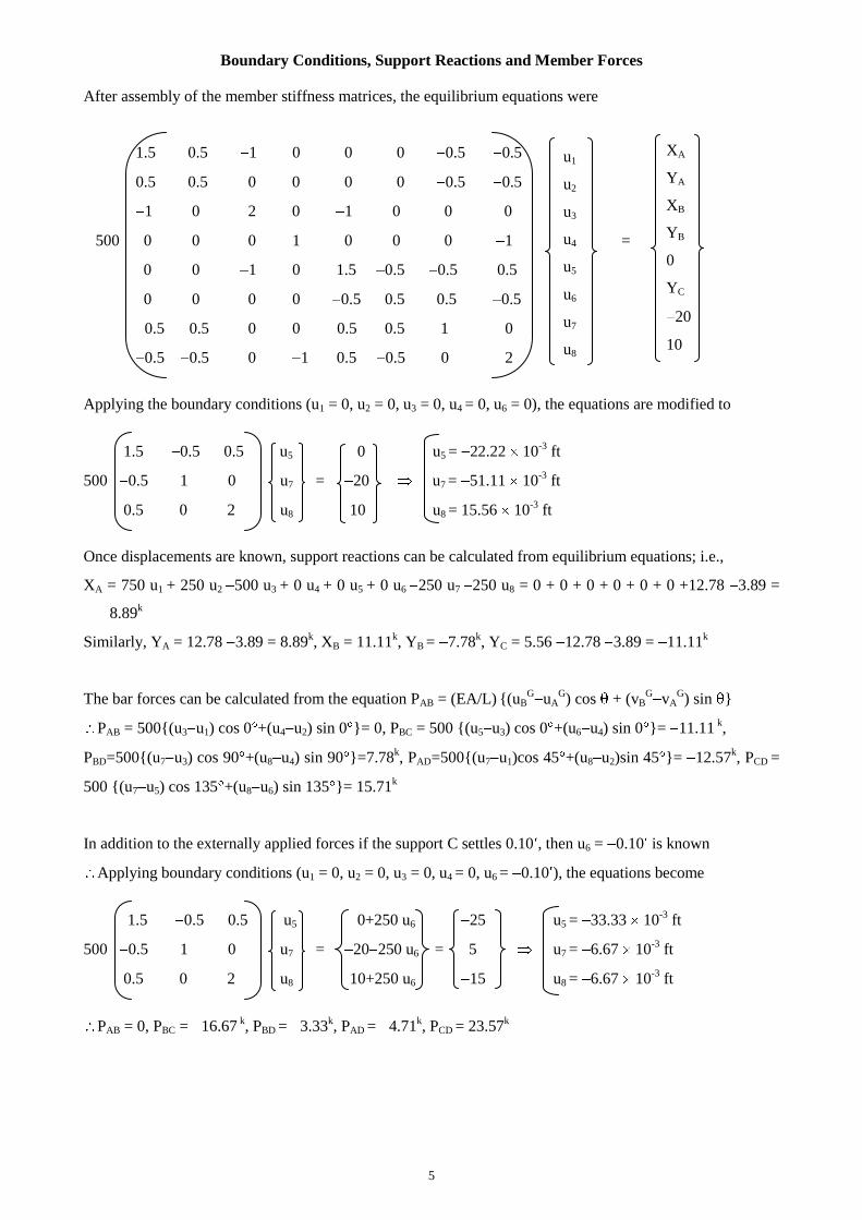
Boundary Conditions, Support Reactions and Member Forces
After assembly of the member stiffness matrices, the equilibrium equations were
1.5 0.5 1 0 0 0 0.5 0.5
0.5 0.5 0 0 0 0 0.5 0.5
1 0 2 0 1 0 0 0
500 0 0 0 1 0 0 0 1 =
0 0 1 0 1.5 0.5 0.5 0.5
0 0 0 0 0.5 0.5 0.5 0.5
0.5 0.5 0 0 0.5 0.5 1 0
0.5 0.5 0 1 0.5 0.5 0 2
Applying the boundary conditions (u1 = 0, u2 = 0, u3 = 0, u4 = 0, u6 = 0), the equations are modified to
1.5 0.5 0.5 u5 0 u5 = 22.22 10-3
ft
500 0.5 1 0 u7 = 20 u7 = 51.11 10-3
ft
0.5 0 2 u8 10 u8 = 15.56 10-3
ft
Once displacements are known, support reactions can be calculated from equilibrium equations; i.e.,
XA = 750 u1 + 250 u2 500 u3 + 0 u4 + 0 u5 + 0 u6 250 u7 250 u8 = 0 + 0 + 0 + 0 + 0 + 0 +12.78 3.89 =
8.89k
Similarly, YA = 12.78 3.89 = 8.89k, XB = 11.11
k, YB = 7.78
k, YC = 5.56 12.78 3.89 = 11.11
k
The bar forces can be calculated from the equation PAB = (EA/L) {(uBG
uAG) cos + (vB
GvA
G) sin }
PAB = 500{(u3 u1) cos 0 +(u4 u2) sin 0 }= 0, PBC = 500 {(u5 u3) cos 0 +(u6 u4) sin 0 }= 11.11 k,
PBD=500{(u7 u3) cos 90 +(u8 u4) sin 90 }=7.78k, PAD=500{(u7 u1)cos 45 +(u8 u2)sin 45 }= 12.57
k, PCD =
500 {(u7 u5) cos 135 +(u8 u6) sin 135 }= 15.71k
In addition to the externally applied forces if the support C settles 0.10 , then u6 = 0.10 is known
Applying boundary conditions (u1 = 0, u2 = 0, u3 = 0, u4 = 0, u6 = 0.10 ), the equations become
1.5 0.5 0.5 u5 0+250 u6 25 u5 = 33.33 10-3
ft
500 0.5 1 0 u7 = 20 250 u6 = 5 u7 = 6.67 10-3
ft
0.5 0 2 u8 10+250 u6 15 u8 = 6.67 10-3
ft
PAB = 0, PBC = 16.67 k, PBD = 3.33
k, PAD = 4.71
k, PCD = 23.57
k
u1
u2
u3
u4
u5
u6
u7
u8
XA
YA
XB
YB
0
YC
20
10
6
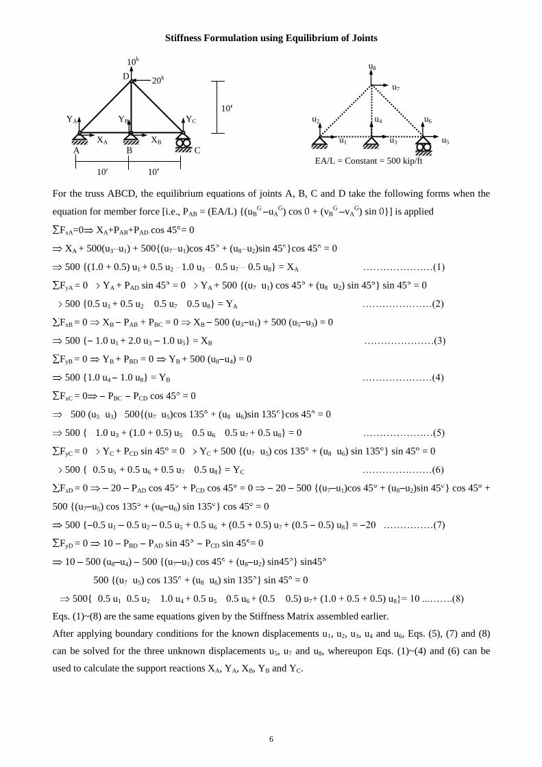
Stiffness Formulation using Equilibrium of Joints
u8
D
u7
10
YA YB YC u2 u4 u6
XA XB u1 u3 u5
A B C
EA/L = Constant = 500 kip/ft
10 10
For the truss ABCD, the equilibrium equations of joints A, B, C and D take the following forms when the
equation for member force [i.e., PAB = (EA/L) {(uBG
uAG) cos + (vB
G vA
G) sin }] is applied
FxA=0 XA+PAB+PAD cos 45 = 0
XA + 500(u3 u1) + 500{(u7 u1)cos 45 + (u8 u2)sin 45 }cos 45 = 0
500 {(1.0 + 0.5) u1 + 0.5 u2 1.0 u3 0.5 u7 0.5 u8} = XA …………………(1)
FyA = 0 YA + PAD sin 45 = 0 YA + 500 {(u7 u1) cos 45 + (u8 u2) sin 45 } sin 45 = 0
500 {0.5 u1 + 0.5 u2 0.5 u7 0.5 u8} = YA …………………(2)
FxB = 0 XB PAB + PBC = 0 XB 500 (u3 u1) + 500 (u5 u3) = 0
500 { 1.0 u1 + 2.0 u3 1.0 u5} = XB …………………(3)
FyB = 0 YB + PBD = 0 YB + 500 (u8 u4) = 0
500 {1.0 u4 1.0 u8} = YB …………………(4)
FxC = 0 PBC PCD cos 45 = 0
500 (u5 u3) 500{(u7 u5)cos 135 + (u8 u6)sin 135 }cos 45 = 0
500 { 1.0 u3 + (1.0 + 0.5) u5 0.5 u6 0.5 u7 + 0.5 u8} = 0 …………………(5)
FyC = 0 YC + PCD sin 45 = 0 YC + 500 {(u7 u5) cos 135 + (u8 u6) sin 135 } sin 45 = 0
500 { 0.5 u5 + 0.5 u6 + 0.5 u7 0.5 u8} = YC …………………(6)
FxD = 0 20 PAD cos 45 + PCD cos 45 = 0 20 500 {(u7 u1)cos 45 + (u8 u2)sin 45 } cos 45 +
500 {(u7 u5) cos 135 + (u8 u6) sin 135 } cos 45 = 0
500 { 0.5 u1 0.5 u2 0.5 u5 + 0.5 u6 + (0.5 + 0.5) u7 + (0.5 0.5) u8} = 20 ……………(7)
FyD = 0 10 PBD PAD sin 45 PCD sin 45 = 0
10 500 (u8 u4) 500 {(u7 u1) cos 45 + (u8 u2) sin45 } sin45
500 {(u7 u5) cos 135 + (u8 u6) sin 135 } sin 45 = 0
500{ 0.5 u1 0.5 u2 1.0 u4 + 0.5 u5 0.5 u6 + (0.5 0.5) u7+ (1.0 + 0.5 + 0.5) u8}= 10 ...…….(8)
Eqs. (1)~(8) are the same equations given by the Stiffness Matrix assembled earlier.
After applying boundary conditions for the known displacements u1, u2, u3, u4 and u6, Eqs. (5), (7) and (8)
can be solved for the three unknown displacements u5, u7 and u8, whereupon Eqs. (1)~(4) and (6) can be
used to calculate the support reactions XA, YA, XB, YB and YC.
20k
10k
7
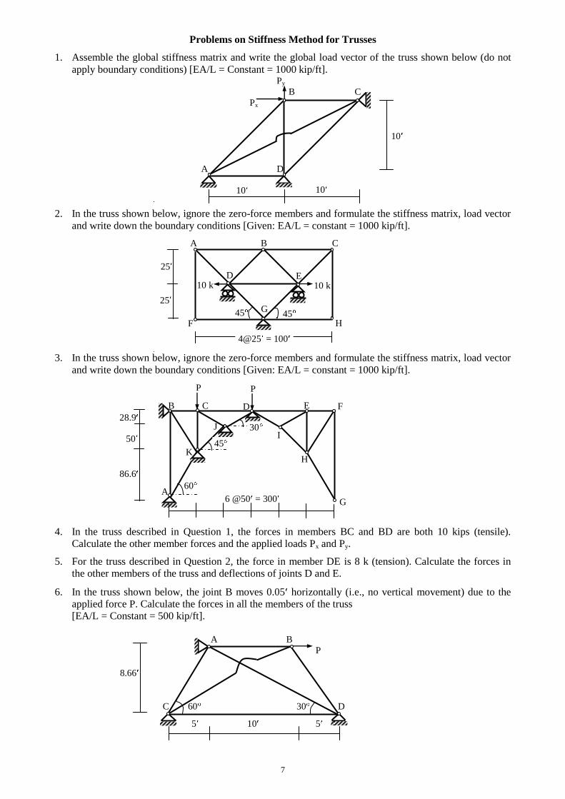
Problems on Stiffness Method for Trusses
1. Assemble the global stiffness matrix and write the global load vector of the truss shown below (do not
apply boundary conditions) [EA/L = Constant = 1000 kip/ft]. Py
B C
Px
10
A D
2. In the truss shown below, ignore the zero-force members and formulate the stiffness matrix, load vector
and write down the boundary conditions [Given: EA/L = constant = 1000 kip/ft].
3. In the truss shown below, ignore the zero-force members and formulate the stiffness matrix, load vector
and write down the boundary conditions [Given: EA/L = constant = 1000 kip/ft].
4. In the truss described in Question 1, the forces in members BC and BD are both 10 kips (tensile).
Calculate the other member forces and the applied loads Px and Py.
5. For the truss described in Question 2, the force in member DE is 8 k (tension). Calculate the forces in
the other members of the truss and deflections of joints D and E.
6. In the truss shown below, the joint B moves 0.05 horizontally (i.e., no vertical movement) due to the
applied force P. Calculate the forces in all the members of the truss
[EA/L = Constant = 500 kip/ft].
A B
P
8.66
C 60 30 D
5 10 5
45 45
10 k
A B C
F
D E
H
G
4@25 = 100
10 k
25
25
P P
A G
B C D E F
K
J I
H
6 @50 = 300
86.6
50
28.9 30
45
60
10 10
8
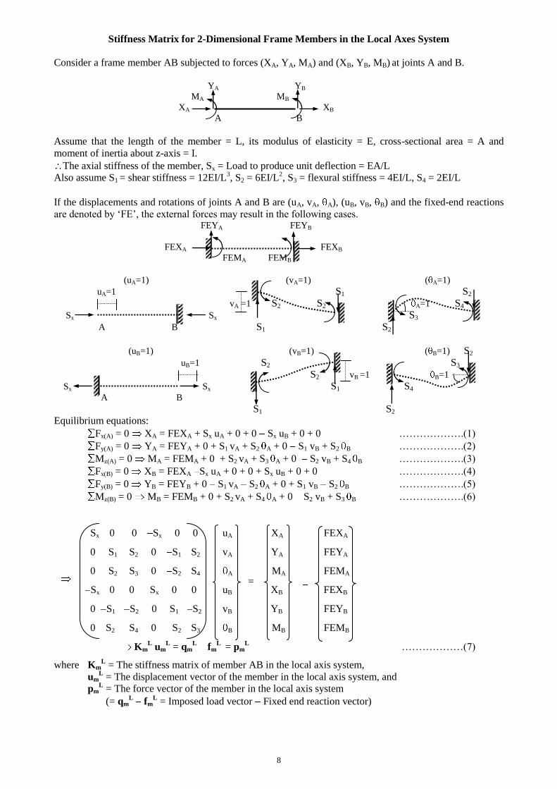
Stiffness Matrix for 2-Dimensional Frame Members in the Local Axes System
Consider a frame member AB subjected to forces (XA, YA, MA) and (XB, YB, MB) at joints A and B.
YA YB
MA MB
XA XB A B
Assume that the length of the member = L, its modulus of elasticity = E, cross-sectional area = A and
moment of inertia about z-axis = I.
The axial stiffness of the member, Sx = Load to produce unit deflection = EA/L
Also assume S1 = shear stiffness = 12EI/L3, S2 = 6EI/L
2, S3 = flexural stiffness = 4EI/L, S4 = 2EI/L
If the displacements and rotations of joints A and B are (uA, vA, A), (uB, vB, B) and the fixed-end reactions
are denoted by ‘FE’, the external forces may result in the following cases. FEYA FEYB
FEXA FEXB
FEMA FEMB
(uA=1) (vA=1) ( A=1)
uA=1 S1 S2
vA =1 S2 S2 A=1 S4
Sx Sx S3
A B S1 S2
(uB=1) (vB=1) ( B=1) S2
uB=1 S2 S3
S2 vB =1 B=1
Sx Sx S1 S4
A B S1 S2
Equilibrium equations:
Fx(A) = 0 XA = FEXA + Sx uA + 0 + 0 Sx uB + 0 + 0 ……………….(1)
Fy(A) = 0 YA = FEYA + 0 + S1 vA + S2 A + 0 S1 vB + S2 B ……………….(2)
Mz(A) = 0 MA = FEMA + 0 + S2 vA + S3 A + 0 S2 vB + S4 B ……………….(3)
Fx(B) = 0 XB = FEXA Sx uA + 0 + 0 + Sx uB + 0 + 0 ……………….(4)
Fy(B) = 0 YB = FEYB + 0 S1 vA S2 A + 0 + S1 vB S2 B ……………….(5)
Mz(B) = 0 MB = FEMB + 0 + S2 vA + S4 A + 0 S2 vB + S3 B ……………….(6)
Sx 0 0 Sx 0 0 uA XA FEXA
0 S1 S2 0 S1 S2 vA YA FEYA
0 S2 S3 0 S2 S4 A MA FEMA
Sx 0 0 Sx 0 0 uB XB FEXB
0 S1 S2 0 S1 S2 vB YB FEYB
0 S2 S4 0 S2 S3 B MB FEMB
KmL um
L = qm
L fm
L = pm
L ………………(7)
where KmL = The stiffness matrix of member AB in the local axis system,
umL = The displacement vector of the member in the local axis system, and
pmL = The force vector of the member in the local axis system
(= qmL fm
L = Imposed load vector Fixed end reaction vector)
=
9
Transformation of Stiffness Matrix from Local to Global Axes
The member matrices formed in the local axes system can be transformed into the global axes system by
considering the angles they make with the horizontal. The local displacements/rotations and global
displacements/rotations are related by the following equations. vB
G
vBL uB
L
B uBG
BL, B
G
vAG
vAL
A uAG
uAL
AL, A
G
Local and global joint displacements and rotations of a frame member
uAL = uA
G cos + vA
G sin …………………(8)
vAL = uA
G sin + vA
G cos …………………(9)
AL = A
G ..………………(10)
uBL = uB
G cos + vB
G sin ………………..(11)
vBL = uB
G sin + vB
G cos ………………..(12)
BL = B
G ………………..(13)
In matrix form, using C = cos , S = sin
uAL C S 0 0 0 0 uA
G
vAL S C 0 0 0 0 vA
G
AL 0 0 1 0 0 0 A
G
uBL 0 0 0 C S 0 uB
G
vBL 0 0 0 S C 0 vB
G
BL 0 0 0 0 0 1 B
G
umL = Tm um
G …………………(14)
where Tm is the transformation matrix for member AB, which connects the displacement vector umL in the
local axes of AB with the displacement vector umG in the global axes.
A similar expression can be obtained for the force vectors pmL and pm
G; i.e.,
pmL = Tm pm
G …………………(15)
Eq. (7) can be rewritten as KmL Tm um
G = Tm pm
G …………….……(16)
(Tm1 Km
L Tm) um
G = pm
G
(TmT Km
L Tm) um
G = pm
G ...………….……(17)
where TmT is the transpose of the transformation matrix Tm, which is also = Tm
1
If (TmT Km
L Tm) is written as Km
G, the member stiffness matrix in the global axis system, then
KmG um
G = pm
G ...………….……(18)
=
10
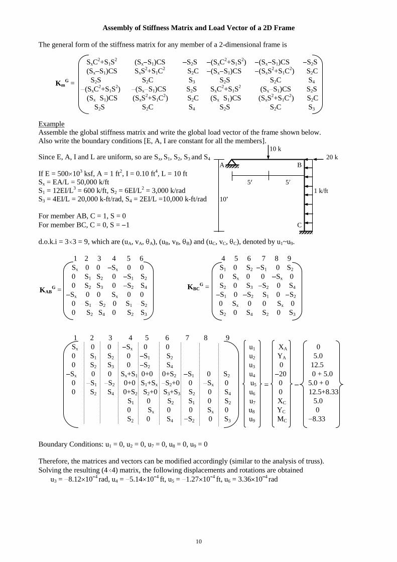
Assembly of Stiffness Matrix and Load Vector of a 2D Frame
The general form of the stiffness matrix for any member of a 2-dimensional frame is
SxC2+S1S
2 (Sx S1)CS S2S (SxC
2+S1S
2) (Sx S1)CS S2S
(Sx S1)CS SxS2+S1C
2 S2C (Sx S1)CS (SxS
2+S1C
2) S2C
S2S S2C
S3 S2S S2C S4
(SxC2+S1S
2) (Sx S1)CS S2S SxC
2+S1S
2 (Sx S1)CS S2S
(Sx S1)CS (SxS2+S1C
2)
S2C (Sx S1)CS (SxS
2+S1C
2) S2C
S2S S2C
S4 S2S S2C S3
Example
Assemble the global stiffness matrix and write the global load vector of the frame shown below.
Also write the boundary conditions [E, A, I are constant for all the members]. 10 k
Since E, A, I and L are uniform, so are Sx, S1, S2, S3 and S4 20 k A B
If E = 500 103 ksf, A = 1 ft
2, I = 0.10 ft
4, L = 10 ft
Sx = EA/L = 50,000 k/ft 5 5
S1 = 12EI/L3 = 600 k/ft, S2 = 6EI/L
2 = 3,000 k/rad 1 k/ft
S3 = 4EI/L = 20,000 k-ft/rad, S4 = 2EI/L =10,000 k-ft/rad 10
For member AB, C = 1, S = 0
For member BC, C = 0, S = 1 C
d.o.k.i = 3 3 = 9, which are (uA, vA, A), (uB, vB, B) and (uC, vC, C), denoted by u1~u9.
1 2 3 4 5 6 4 5 6 7 8 9
Sx 0 0 Sx 0 0 S1 0 S2 S1 0 S2
0 S1 S2 0 S1 S2 0 Sx 0 0 Sx 0
0 S2 S3 0 S2 S4 S2 0 S3 S2 0 S4
Sx 0 0 Sx 0 0 S1 0 S2 S1 0 S2
0 S1 S2 0 S1 S2 0 Sx 0 0 Sx 0
0 S2 S4 0 S2 S3 S2 0 S4 S2 0 S3
1 2 3 4 5 6 7 8 9
Sx 0 0 Sx 0 0 u1 XA 0
0 S1 S2 0 S1 S2 u2 YA 5.0
0 S2 S3 0 S2 S4 u3 0 12.5
Sx 0 0 Sx+S1 0+0 0+S2 S1 0 S2 u4 20 0 + 5.0
0 S1 S2 0+0 S1+Sx S2+0 0 Sx 0 u5 0 5.0 + 0
0 S2 S4 0+S2 S2+0 S3+S3 S2 0 S4 u6 0 12.5+8.33
S1 0 S2 S1 0 S2 u7 XC 5.0
0 Sx 0 0 Sx 0 u8 YC 0
S2 0 S4 S2 0 S3 u9 MC 8.33
Boundary Conditions: u1 = 0, u2 = 0, u7 = 0, u8 = 0, u9 = 0
Therefore, the matrices and vectors can be modified accordingly (similar to the analysis of truss).
Solving the resulting (4 4) matrix, the following displacements and rotations are obtained
u3 = 8.12 104 rad, u4 = 5.14 10
4 ft, u5 = 1.27 10
4 ft, u6 = 3.36 10
4 rad
KmG =
KABG = KBC
G =
=

11
Stiffness Method for 2-D Frame neglecting Axial Deformations
If axial deformations are neglected in the problem shown before, the displacements u4 and u5 are zero and
the only unknown displacements are the rotations u3 and u6. In that case, the modified equilibrium equations
are
S3 u3 + S4 u6 = 12.5 20 103 u3 + 10 10
3 u6 = 12.5
and S4 u3 + 2S3 u6 = 4.17 10 103 u3 + 40 10
3 u6 = 4.17
[Note: S1 = 600 k/ft, S2 = 3,000 k/rad, S3 = 20,000 k-ft/rad, S4 = 10,000 k-ft/rad]
Solving, u3 = 7.74 104 rad, u6 = 2.98 10
4 rad [instead of 8.12 10
4, 3.36 10
4 found before]
If the axial deformations are neglected, the calculations and formulations are much simplified without
significant loss of accuracy.
Neglecting the axial deformations, the earlier problem can be formulated as shown below
u3 10 k u6
A B Here, d.o.k.i. = 2
20 k There can be three cases of response
(i) Case0: The fixed-end reactions
(ii) Case1: The reactions due to u3
(iii) Case2: The reactions due to u6
C
5 k 5 k S2
12.5 k 12.5 k S4 S3
25 k
8.33 k S3 S4
S2 S2 S3
8.33 k S4
Case 0 (FER) 5 k Case 1 (u3 = 1) Case 2 (u6 = 1) S2
Equilibrium equations:
Mz(A) = 0 12.5 + S3 u3 + S4 u6 = 0 20 103 u3 + 10 10
3 u6 = 12.5
Mz(B) = 0 12.5 + 8.33 + S4 u3 + (S3+S3) u6 = 0 10 103 u3 + 40 10
3 u6 = 4.17
Solving the two equations, u3 = 7.74 104
rad, u6 = 2.98 104 rad
Calculation of Internal Forces (SF and BM):
SF(A) = 5 + S2 u3 + S2 u6 = 5 + 3,000 ( 7.74 104) + 3,000 (2.98 10
4) = 3.54 k
SF(B) (in AB) = 5 S2 u3 S2 u6 = 5 3,000 ( 7.74 104) 3,000 (2.98 10
4) = 6.46 k
SF(B) (in BC) = 25 + 0 + S2 u6 = 25 + 3,000 (2.98 104) = 25.89 k
SF(C) (in BC) = 5 + 0 S2 u6 = 5 3,000 (2.98 104) = 4.11 k should be zero
BM(A) = 12.5 + S3 u3 + S4 u6 = 12.5 + 20,000 ( 7.74 104) + 10,000 (2.98 10
4) = 0
BM(B) (in AB) = 12.5+ S4 u3 + S3 u6 = 12.5+ 10,000 ( 7.74 104)+ 20,000 (2.98 10
4) = 14.28 k
BM(B) (in BC) = 8.33 + 0 + S3 u6 = 8.33 + 20,000 (2.98 104) = 14.29 k
BM(C) = 8.33 + 0 + S4 u6 = 8.33 + 10,000 (2.98 104) = 5.35 k should be equal
S2
S2
12
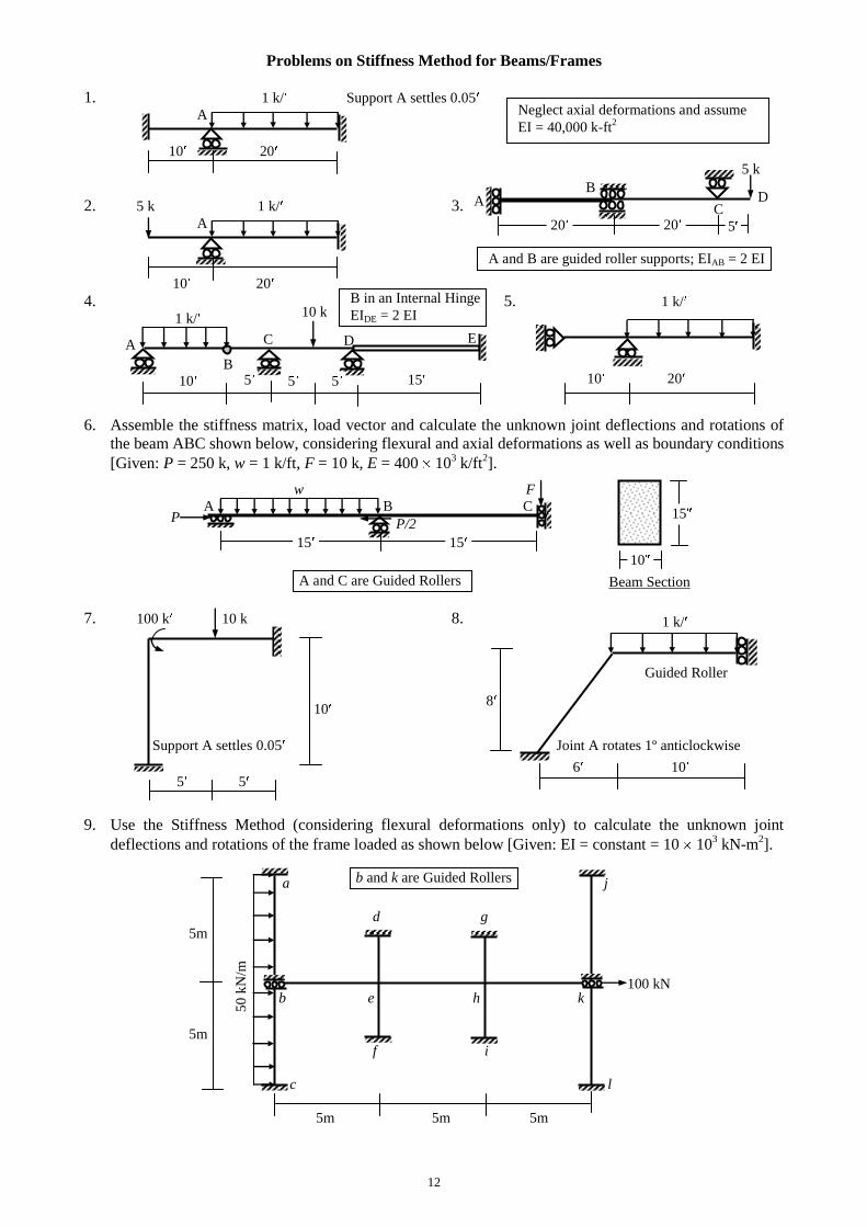
Problems on Stiffness Method for Beams/Frames
1. 1 k/ Support A settles 0.05 A
10 20
2. 5 k 1 k/ 3. A
10 20
4. 5. 1 k/
10 20
6. Assemble the stiffness matrix, load vector and calculate the unknown joint deflections and rotations of
the beam ABC shown below, considering flexural and axial deformations as well as boundary conditions
[Given: P = 250 k, w = 1 k/ft, F = 10 k, E = 400 103 k/ft
2].
w F
A B C
Beam Section
7. 100 k 10 k 8.
Guided Roller
10
Support A settles 0.05 Joint A rotates 1º anticlockwise
5 5
9. Use the Stiffness Method (considering flexural deformations only) to calculate the unknown joint
deflections and rotations of the frame loaded as shown below [Given: EI = constant = 10 103 kN-m
2].
a j
d g
5m
100 kN
5m
f i
c l
5m 5m 5m
D C
B A
A and B are guided roller supports; EIAB = 2 EI
20 5
5 k
20
8
6 10
1 k/
B
A
B in an Internal Hinge
EIDE = 2 EI
C
10 k
5 15
D
1 k/
10 5 5
E
Neglect axial deformations and assume
EI = 40,000 k-ft2
b and k are Guided Rollers
b e h k
50
kN
/m
A and C are Guided Rollers
P
10
15
15 15
P/2
13
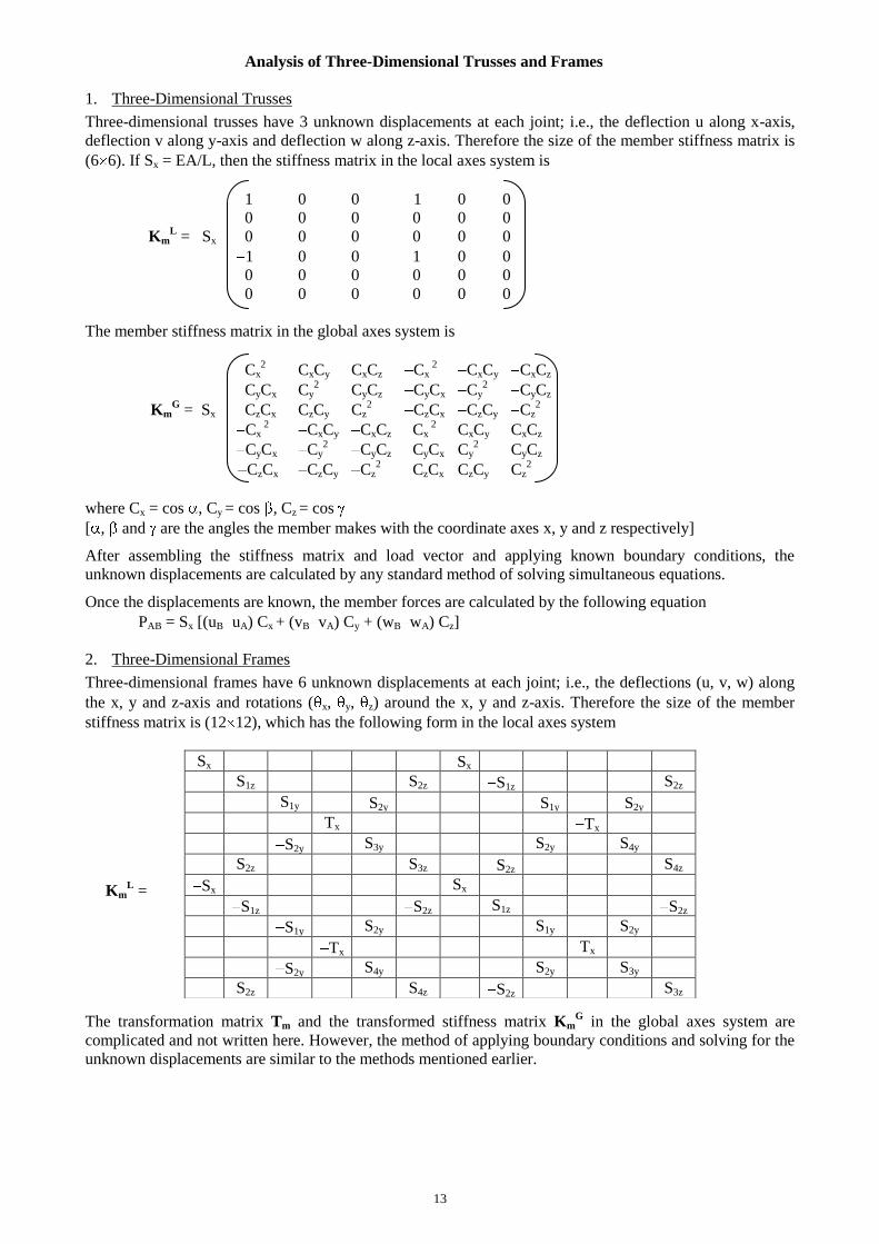
Analysis of Three-Dimensional Trusses and Frames
1. Three-Dimensional Trusses
Three-dimensional trusses have 3 unknown displacements at each joint; i.e., the deflection u along x-axis,
deflection v along y-axis and deflection w along z-axis. Therefore the size of the member stiffness matrix is
(6 6). If Sx = EA/L, then the stiffness matrix in the local axes system is
1 0 0 1 0 0
0 0 0 0 0 0
KmL = Sx 0 0 0 0 0 0
1 0 0 1 0 0
0 0 0 0 0 0
0 0 0 0 0 0
The member stiffness matrix in the global axes system is
Cx2 CxCy CxCz Cx
2 CxCy CxCz
CyCx Cy2 CyCz CyCx Cy
2 CyCz
KmG = Sx CzCx CzCy Cz
2 CzCx CzCy Cz
2
Cx 2 CxCy CxCz Cx
2 CxCy CxCz
CyCx Cy2 CyCz CyCx Cy
2 CyCz
CzCx CzCy Cz2 CzCx CzCy Cz
2
where Cx = cos , Cy = cos , Cz = cos
[ , and are the angles the member makes with the coordinate axes x, y and z respectively]
After assembling the stiffness matrix and load vector and applying known boundary conditions, the
unknown displacements are calculated by any standard method of solving simultaneous equations.
Once the displacements are known, the member forces are calculated by the following equation
PAB = Sx [(uB uA) Cx + (vB vA) Cy + (wB wA) Cz]
2. Three-Dimensional Frames
Three-dimensional frames have 6 unknown displacements at each joint; i.e., the deflections (u, v, w) along
the x, y and z-axis and rotations ( x, y, z) around the x, y and z-axis. Therefore the size of the member
stiffness matrix is (12 12), which has the following form in the local axes system
KmL =
The transformation matrix Tm and the transformed stiffness matrix KmG in the global axes system are
complicated and not written here. However, the method of applying boundary conditions and solving for the
unknown displacements are similar to the methods mentioned earlier.
Sx Sx
S1z S2z S1z S2z
S1y S2y S1y S2y
Tx Tx
S2y S3y S2y S4y
S2z S3z S2z S4z
Sx Sx
S1z S2z S1z S2z
S1y S2y S1y S2y
Tx Tx
S2y S4y S2y S3y
S2z S4z S2z S3z
14
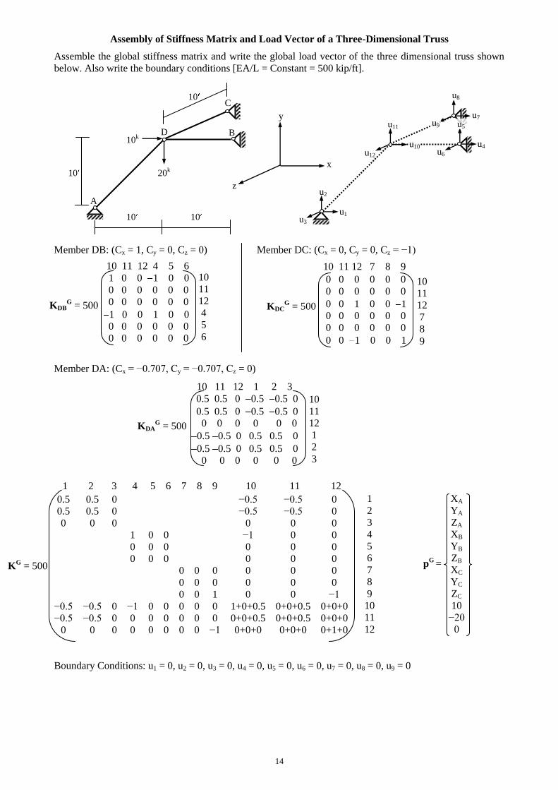
Assembly of Stiffness Matrix and Load Vector of a Three-Dimensional Truss
Assemble the global stiffness matrix and write the global load vector of the three dimensional truss shown
below. Also write the boundary conditions [EA/L = Constant = 500 kip/ft].
10
10k
10 20k
10 10
Member DB: (Cx = 1, Cy = 0, Cz = 0) Member DC: (Cx = 0, Cy = 0, Cz = −1)
Member DA: (Cx = −0.707, Cy = −0.707, Cz = 0)
0.5 0.5 0 −0.5 −0.5 0
0.5 0.5 0 −0.5 −0.5 0
0 0 0 0 0 0
1 0 0 −1 0 0
0 0 0 0 0 0
0 0 0 0 0 0
0 0 0 0 0 0
0 0 0 0 0 0
0 0 1 0 0 −1
−0.5 −0.5 0 −1 0 0 0 0 0 1+0+0.5 0+0+0.5 0+0+0
−0.5 −0.5 0 0 0 0 0 0 0 0+0+0.5 0+0+0.5 0+0+0
0 0 0 0 0 0 0 0 −1 0+0+0 0+0+0 0+1+0
Boundary Conditions: u1 = 0, u2 = 0, u3 = 0, u4 = 0, u5 = 0, u6 = 0, u7 = 0, u8 = 0, u9 = 0
x
y
z
A
C
B D
u1
u2
u3
u10
u11
u12 u4
u5
u6
u7
u8
u9
1 0 0 1 0 0 0 0 0 0 0 0 0 0 0 0 0 0 1 0 0 1 0 0 0 0 0 0 0 0 0 0 0 0 0 0
KDBG = 500
10 11 12 4 5 6 10
11
12
4
5
6
KDCG = 500
10 11 12 7 8 9
10
11
12
7
8
9
0.5 0.5 0 0.5 0.5 0 0.5 0.5 0 0.5 0.5 0 0 0 0 0 0 0
0.5 0.5 0 0.5 0.5 0 0.5 0.5 0 0.5 0.5 0
0 0 0 0 0 0
KDAG = 500
10 11 12 1 2 3 10
11
12
1
2
3
0 0 0 0 0 0 0 0 0 0 0 0 0 0 1 0 0 1 0 0 0 0 0 0 0 0 0 0 0 0 0 0 1 0 0 1
KG = 500
1 2 3 4 5 6 7 8 9 10 11 12 1
2
3
4
5
6
7
8
9
10
11
12
pG
=
XA
YA
ZA
XB
YB
ZB
XC
YC
ZC
10
−20
0
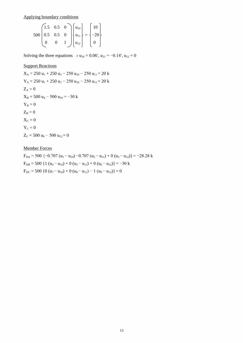
15
Applying boundary conditions
1.5 0.5 0 u10 10
0.5 0.5 0 u11 = −20
0 0 1 u12 0
Solving the three equations u10 = 0.06 , u11 = −0.14 , u12 = 0
Support Reactions
XA = 250 u1 + 250 u2 − 250 u10 − 250 u11 = 20 k
YA = 250 u1 + 250 u2 − 250 u10 − 250 u11 = 20 k
ZA = 0
XB = 500 u4 − 500 u10 = −30 k
YB = 0
ZB = 0
XC = 0
YC = 0
ZC = 500 u9 − 500 u12 = 0
Member Forces
FDA = 500 {−0.707 (u1 − u10) −0.707 (u2 − u11) + 0 (u3 − u12)} = −28.28 k
FDB = 500 {1 (u4 − u10) + 0 (u5 − u11) + 0 (u6 − u12)} = −30 k
FDC = 500 {0 (u7 − u10) + 0 (u8 − u11) − 1 (u9 − u12)} = 0
500
16
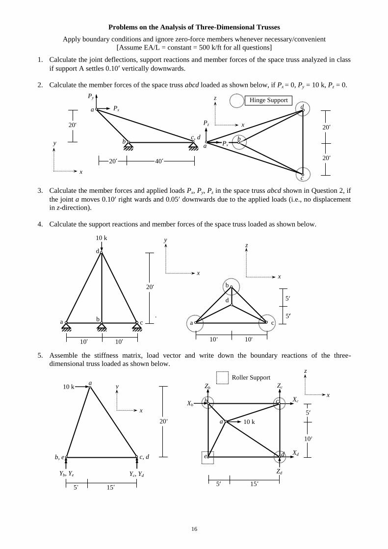
Problems on the Analysis of Three-Dimensional Trusses
Apply boundary conditions and ignore zero-force members whenever necessary/convenient
[Assume EA/L = constant = 500 k/ft for all questions]
1. Calculate the joint deflections, support reactions and member forces of the space truss analyzed in class
if support A settles 0.10 vertically downwards.
2. Calculate the member forces of the space truss abcd loaded as shown below, if Px = 0, Py = 10 k, Pz = 0.
3. Calculate the member forces and applied loads Px, Py, Pz in the space truss abcd shown in Question 2, if
the joint a moves 0.10 right wards and 0.05 downwards due to the applied loads (i.e., no displacement
in z-direction).
4. Calculate the support reactions and member forces of the space truss loaded as shown below.
b
d
.
a c
5. Assemble the stiffness matrix, load vector and write down the boundary reactions of the three-
dimensional truss loaded as shown below.
x
d
a b
c, d
a
y
x
c b a
d
10 k
10 10
20
5
5
z
x
c, d b, e
a 10 k
Yb, Ye Yc, Yd
5 15
20
5
10
y
x
z
x
Px
y
20 20
20
b
c
20 40
x
z
a 10 k
d
c
e
b
Roller Support
10 10
5 15
Py
Pz
Px
Hinge Support
Xb
Zb
Xc
Zc
Xd
Zd
17
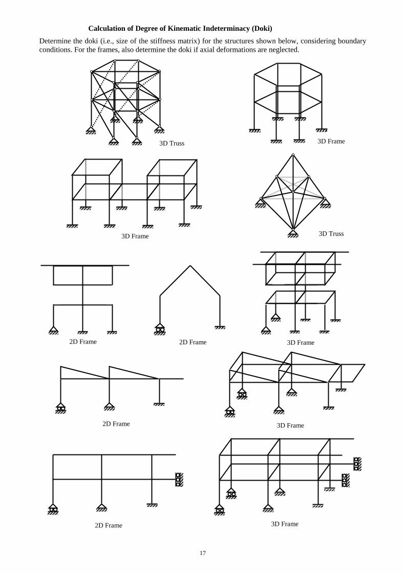
Calculation of Degree of Kinematic Indeterminacy (Doki)
Determine the doki (i.e., size of the stiffness matrix) for the structures shown below, considering boundary
conditions. For the frames, also determine the doki if axial deformations are neglected.
3D Truss 3D Frame
2D Frame 3D Frame 2D Frame
3D Frame 3D Truss
2D Frame 3D Frame
2D Frame 3D Frame
18
Energy Formulation of Geometric Nonlinearity
Linear structural analysis is based on the assumption of small deformations and linear elastic behavior of
materials. The analysis is performed on the initial undeformed shape of the structure. As the applied loads
increase, this assumption is no longer accurate, because the deformations may cause significant changes in
the structural shape. Geometric nonlinearity is the change in the elastic load-deformation characteristics of
the structure caused by the change in the structural shape.
Among various types of geometric nonlinearity, the structural instability or moment magnification caused by
large compressive forces, stiffening of structures due to large tensile forces, change in structural parameters
due to applied dynamic loads are significant. Rather than using equilibrium equations, it is often more
convenient to formulate geometrically nonlinear problems by the Method of Virtual Work.
Method of Virtual Work
Another way of representing Newton’s equation of equilibrium is by energy methods, which is based on the
law of conservation of energy. According to the principle of virtual work, if a system in equilibrium is
subjected to virtual displacements u, the virtual work done by the external forces ( WE) is equal to the
virtual work done by the internal forces ( WI)
WI = WE ...…………………(1)
where the symbol is used to indicate ‘virtual’. This term is used to indicate hypothetical increments of
displacements and works that are assumed to happen in order to formulate the problem.
Energy Formulation and Buckling of Beams-columns
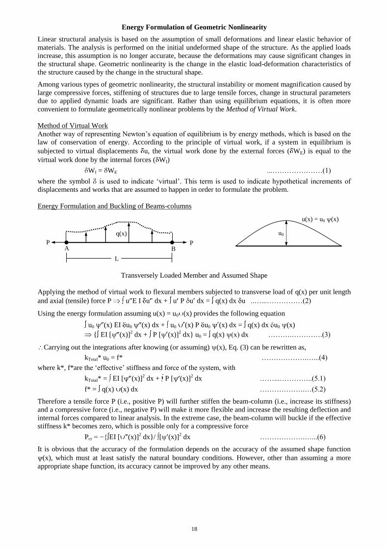
Transversely Loaded Member and Assumed Shape
Applying the method of virtual work to flexural members subjected to transverse load of q(x) per unit length
and axial (tensile) force P u E I u dx + u P u dx = q(x) dx u ..…...……………(2)
Using the energy formulation assuming u(x) = u0 (x) provides the following equation
u0 (x) EI u0 (x) dx + u0 (x) P u0 (x) dx = q(x) dx u0 (x)
{ EI [ (x)]2 dx + P [ (x)]
2 dx} u0 = q(x) (x) dx ……….………….(3)
Carrying out the integrations after knowing (or assuming) (x), Eq. (3) can be rewritten as,
kTotal* u0 = f* ……………….…...(4)
where k*, f*are the ‘effective’ stiffness and force of the system, with
kTotal* = EI [ (x)]2 dx + P [ (x)]
2 dx ……...…………..(5.1)
f* = q(x) (x) dx ……………….…(5.2)
Therefore a tensile force P (i.e., positive P) will further stiffen the beam-column (i.e., increase its stiffness)
and a compressive force (i.e., negative P) will make it more flexible and increase the resulting deflection and
internal forces compared to linear analysis. In the extreme case, the beam-column will buckle if the effective
stiffness k* becomes zero, which is possible only for a compressive force
Pcr = −{ EI [ (x)]2 dx}/ [ (x)]
2 dx ……………….…...(6)
It is obvious that the accuracy of the formulation depends on the accuracy of the assumed shape function
(x), which must at least satisfy the natural boundary conditions. However, other than assuming a more
appropriate shape function, its accuracy cannot be improved by any other means.
u0 q(x)
A B P P
u(x) = u0 (x)
L
19
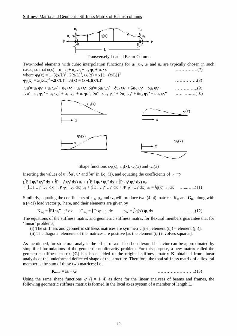
Stiffness Matrix and Geometric Stiffness Matrix of Beams-columns
u1 u3
u2 q(x) u4
L
Transversely Loaded Beam-Column
Two-noded elements with cubic interpolation functions for u1, u2, u3 and u4 are typically chosen in such
cases, so that u(x) = u1 1 + u2 2 + u3 3 + u4 4 ……………(7)
where 1(x) = 1 3(x/L)2 +2(x/L)
3, 2(x) = x{1 (x/L)}
2
3(x) = 3(x/L)2
2(x/L)3, 4(x) = (x L)(x/L)
2 ……………(8)
u = u1 1 + u2 2 + u3 3 + u4 4 ; u = u1 1
+ u2 2 + u3 3 + u4 4 .……….…..(9)
u = u1 1 + u2 2 + u3 3 + u4 4 ; u = u1 1
+ u2 2 + u3 3 + u4 4 .…...…..…(10)
1(x)
2(x)
3(x)
4(x)
Shape functions 1(x), 2(x), 3(x) and 4(x)
Inserting the values of u , u , u and u in Eq. (1), and equating the coefficients of 1
( E I 1 1 dx + P 1 1 dx) u1 + ( E I 1 2 dx + P 1 2 dx) u2
+ ( E I 1 3 dx + P 1 3 dx) u3 + ( E I 1 4 dx + P 1 4 dx) u4 = q(x) 1 dx …...…...(11)
Similarly, equating the coefficients of 2, 3 and 4 will produce two (4 4) matrices Km and Gm, along with
a (4 1) load vector pm here, and their elements are given by
Kmij = EI i
j dx Gmij = P i j dx pmi = q(x) i dx ……..…(12)
The equations of the stiffness matrix and geometric stiffness matrix for flexural members guarantee that for
‘linear’ problems,
(i) The stiffness and geometric stiffness matrices are symmetric [i.e., element (i,j) = element (j,i)],
(ii) The diagonal elements of the matrices are positive [as the element (i,i) involves squares].
As mentioned, for structural analysis the effect of axial load on flexural behavior can be approximated by
simplified formulations of the geometric nonlinearity problem. For this purpose, a new matrix called the
geometric stiffness matrix (G) has been added to the original stiffness matrix K obtained from linear
analysis of the undeformed deflected shape of the structure. Therefore, the total stiffness matrix of a flexural
member is the sum of these two matrices; i.e.,
Ktotal = K + G ……………………..(13)
Using the same shape functions i (i = 1~4) as done for the linear analyses of beams and frames, the
following geometric stiffness matrix is formed in the local axes system of a member of length L.
x
x
x
x
P P A B
20
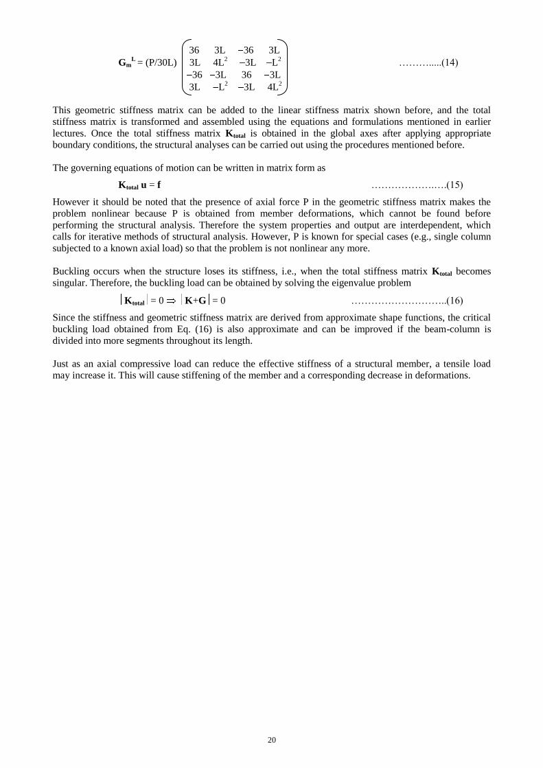
36 3L 36 3L
GmL
= (P/30L) 3L 4L2
3L L2 ……….....(14)
36 3L 36 3L
3L L2
3L 4L2
This geometric stiffness matrix can be added to the linear stiffness matrix shown before, and the total
stiffness matrix is transformed and assembled using the equations and formulations mentioned in earlier
lectures. Once the total stiffness matrix Ktotal is obtained in the global axes after applying appropriate
boundary conditions, the structural analyses can be carried out using the procedures mentioned before.
The governing equations of motion can be written in matrix form as
Ktotal u = f ……………….….(15)
However it should be noted that the presence of axial force P in the geometric stiffness matrix makes the
problem nonlinear because P is obtained from member deformations, which cannot be found before
performing the structural analysis. Therefore the system properties and output are interdependent, which
calls for iterative methods of structural analysis. However, P is known for special cases (e.g., single column
subjected to a known axial load) so that the problem is not nonlinear any more.
Buckling occurs when the structure loses its stiffness, i.e., when the total stiffness matrix Ktotal becomes
singular. Therefore, the buckling load can be obtained by solving the eigenvalue problem
Ktotal = 0 K+G = 0 ………………………..(16)
Since the stiffness and geometric stiffness matrix are derived from approximate shape functions, the critical
buckling load obtained from Eq. (16) is also approximate and can be improved if the beam-column is
divided into more segments throughout its length.
Just as an axial compressive load can reduce the effective stiffness of a structural member, a tensile load
may increase it. This will cause stiffening of the member and a corresponding decrease in deformations.
21
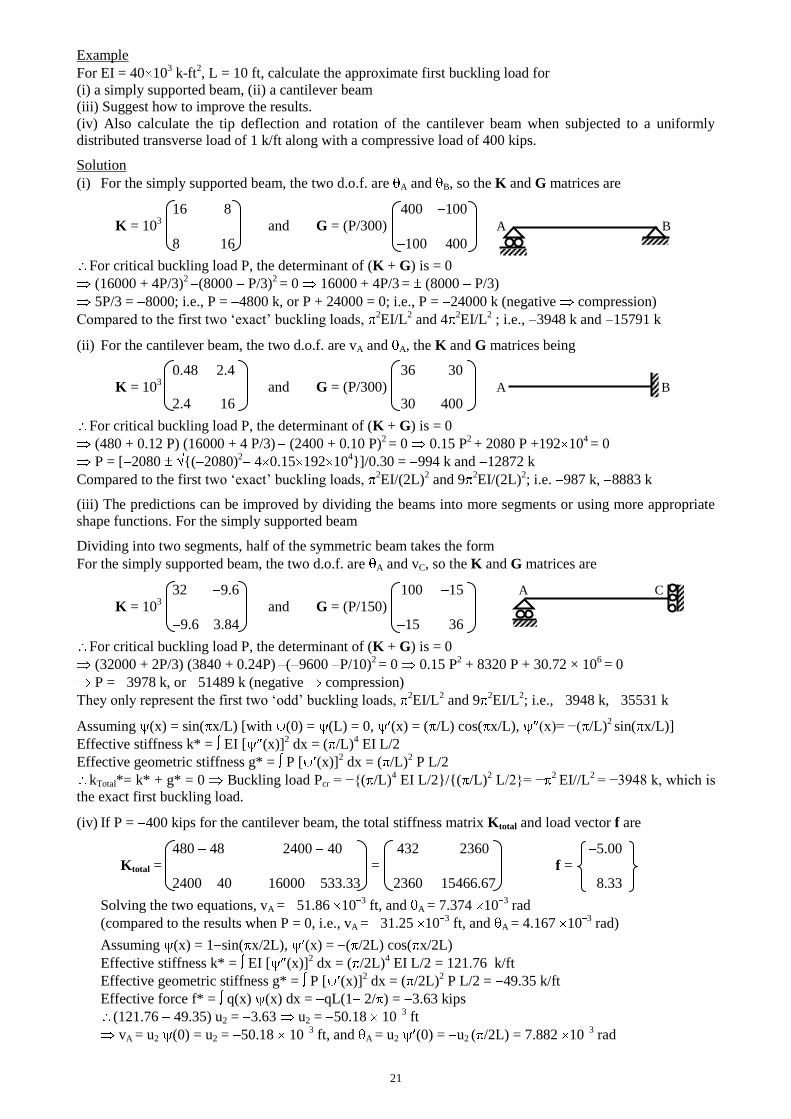
Example
For EI = 40 103 k-ft
2, L = 10 ft, calculate the approximate first buckling load for
(i) a simply supported beam, (ii) a cantilever beam
(iii) Suggest how to improve the results.
(iv) Also calculate the tip deflection and rotation of the cantilever beam when subjected to a uniformly
distributed transverse load of 1 k/ft along with a compressive load of 400 kips.
Solution
(i) For the simply supported beam, the two d.o.f. are A and B, so the K and G matrices are
16 8 400 100
K = 103 and G = (P/300) A B
8 16 100 400
For critical buckling load P, the determinant of (K + G) is = 0
(16000 + 4P/3)2
(8000 P/3)2 = 0 16000 + 4P/3
= (8000 P/3)
5P/3 = 8000; i.e., P = 4800 k, or P + 24000 = 0; i.e., P = 24000 k (negative compression)
Compared to the first two ‘exact’ buckling loads, 2EI/L
2 and 4
2EI/L
2 ; i.e., 3948 k and 15791 k
(ii) For the cantilever beam, the two d.o.f. are vA and A, the K and G matrices being
0.48 2.4 36 30
K = 103 and G = (P/300) A B
2.4 16 30 400
For critical buckling load P, the determinant of (K + G) is = 0
(480 + 0.12 P) (16000 + 4 P/3)
(2400 + 0.10 P)2 = 0 0.15 P
2 + 2080 P +192 10
4 = 0
P = [ 2080 {( 2080)2
4 0.15 192 104}]/0.30 = 994 k and 12872 k
Compared to the first two ‘exact’ buckling loads, 2EI/(2L)
2 and 9
2EI/(2L)
2; i.e. 987 k, 8883 k
(iii) The predictions can be improved by dividing the beams into more segments or using more appropriate
shape functions. For the simply supported beam
Dividing into two segments, half of the symmetric beam takes the form
For the simply supported beam, the two d.o.f. are A and vC, so the K and G matrices are
32 9.6 100 15 A C
K = 103 and G = (P/150)
9.6 3.84 15 36
For critical buckling load P, the determinant of (K + G) is = 0
(32000 + 2P/3) (3840 + 0.24P)
( 9600 P/10)2 = 0 0.15 P
2 + 8320 P + 30.72 × 10
6 = 0
P = 3978 k, or 51489 k (negative compression)
They only represent the first two ‘odd’ buckling loads, 2EI/L
2 and 9
2EI/L
2; i.e., 3948 k, 35531 k
Assuming (x) = sin( x/L) [with (0) = (L) = 0, (x) = ( /L) cos( x/L), (x)= −( /L)2 sin( x/L)]
Effective stiffness k* = EI [ (x)]2 dx = ( /L)
4 EI L/2
Effective geometric stiffness g* = P [ (x)]2 dx = ( /L)
2 P L/2
kTotal*= k* + g* = 0 Buckling load Pcr = −{( /L)4 EI L/2}/{( /L)
2 L/2}= −
2 EI//L
2 = −3948 k, which is
the exact first buckling load.
(iv) If P = 400 kips for the cantilever beam, the total stiffness matrix Ktotal and load vector f are
480 48 2400 40 432 2360 5.00
Ktotal = = f =
2400 40 16000 533.33 2360 15466.67 8.33
Solving the two equations, vA = 51.86 103 ft, and A = 7.374 10
3 rad
(compared to the results when P = 0, i.e., vA = 31.25 103 ft, and A = 4.167 10
3 rad)
Assuming (x) = 1 sin( x/2L), (x) = ( /2L) cos( x/2L)
Effective stiffness k* = EI [ (x)]2 dx = ( /2L)
4 EI L/2 = 121.76 k/ft
Effective geometric stiffness g* = P [ (x)]2 dx = ( /2L)
2 P L/2 = 49.35 k/ft
Effective force f* = q(x) (x) dx = qL(1 2/ ) = 3.63 kips
(121.76 49.35) u2 = 3.63 u2 = 50.18 103 ft
vA = u2 (0) = u2 = 50.18 103 ft, and A = u2 (0) = u2 ( /2L) = 7.882 10
3 rad
22
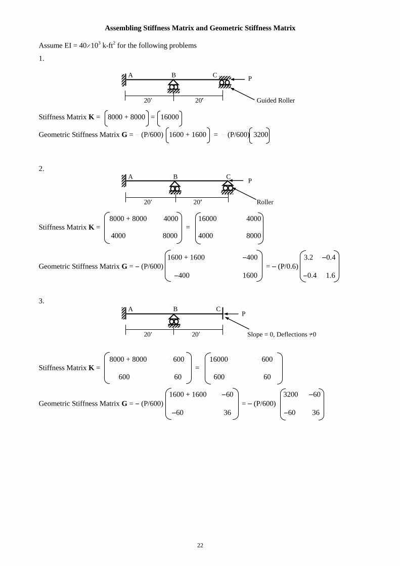
Assembling Stiffness Matrix and Geometric Stiffness Matrix
Assume EI = 40 103 k-ft
2 for the following problems
1.
A B C
20 20 Guided Roller
Stiffness Matrix K = 8000 + 8000 = 16000
Geometric Stiffness Matrix G = (P/600) 1600 + 1600 = (P/600) 3200
2. A B C
20 20 Roller
8000 + 8000 4000
16000 4000
Stiffness Matrix K = =
4000 8000
4000 8000
1600 + 1600
400 3.2 0.4
Geometric Stiffness Matrix G = (P/600) = (P/0.6)
400
1600
0.4 1.6
3. A B C
20 20 Slope = 0, Deflections 0
8000 + 8000 600
16000 600
Stiffness Matrix K = =
600 60
600 60
1600 + 1600
60 3200 60
Geometric Stiffness Matrix G = (P/600) = (P/600)
60
36
60 36
P
P
P
23
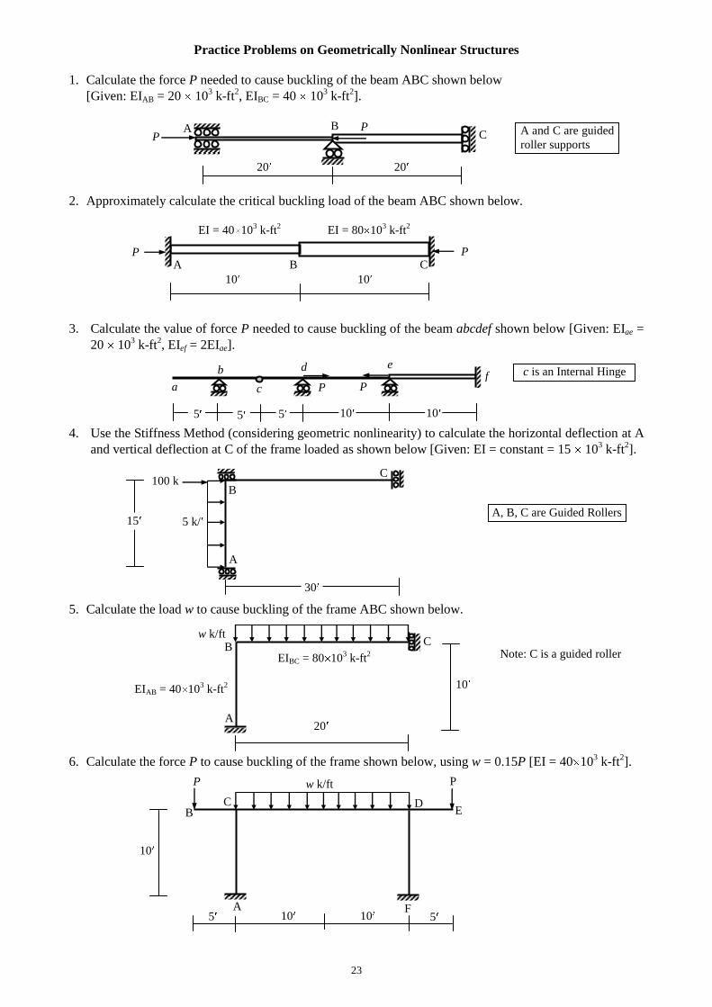
Practice Problems on Geometrically Nonlinear Structures
1. Calculate the force P needed to cause buckling of the beam ABC shown below [Given: EIAB = 20 10
3 k-ft
2, EIBC = 40 10
3 k-ft
2].
2. Approximately calculate the critical buckling load of the beam ABC shown below.
EI = 40 103 k-ft
2 EI = 80 10
3 k-ft
2
A B C
10 10
3. Calculate the value of force P needed to cause buckling of the beam abcdef shown below [Given: EIae =
20 103 k-ft
2, EIef = 2EIae].
4. Use the Stiffness Method (considering geometric nonlinearity) to calculate the horizontal deflection at A
and vertical deflection at C of the frame loaded as shown below [Given: EI = constant = 15 103 k-ft
2].
5. Calculate the load w to cause buckling of the frame ABC shown below.
Note: C is a guided roller
6. Calculate the force P to cause buckling of the frame shown below, using w = 0.15P [EI = 40 103 k-ft
2].
w k/ft
A
B C
EIBC = 80 103 k-ft
2
20
10 EIAB = 40 103 k-ft
2
P P
A
C D
5
10
P
B
10 10
E
F 5
P w k/ft
B
5 k/
30
15
c is an Internal Hinge
5 10 5 5 10
b
a c
d f
P P
A
100 k
A, B, C are Guided Rollers
C
e
20 20
C B A
P P A and C are guided
roller supports
24
Material Nonlinearity and Plastic Moment
As mentioned in the previous section, structural properties cannot be assumed to remain constant in many
practical situations. In addition to the geometric nonlinearity that may lead to instability of structures with
linearly materials properties, the variation in material properties itself can make the structural analysis
nonlinear. For example, yielding of the structural materials, a likely situation in a severe loading conditions
or ground vibrations, may alter the stiffness properties, which needs to be updated with structural
deformations.
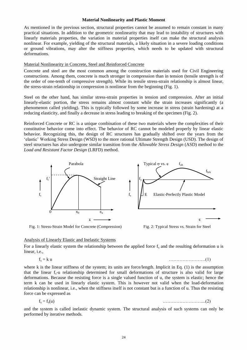
Material Nonlinearity in Concrete, Steel and Reinforced Concrete
Concrete and steel are the most common among the construction materials used for Civil Engineering
constructions. Among them, concrete is much stronger in compression than in tension (tensile strength is of
the order of one-tenth of compressive strength). While its tensile stress-strain relationship is almost linear,
the stress-strain relationship in compression is nonlinear from the beginning (Fig. 1).
Steel on the other hand, has similar stress-strain properties in tension and compression. After an initial
linearly-elastic portion, the stress remains almost constant while the strain increases significantly (a
phenomenon called yielding). This is typically followed by some increase in stress (strain hardening) at a
reducing elasticity, and finally a decrease in stress leading to breaking of the specimen (Fig. 2).
Reinforced Concrete or RC is a unique combination of these two materials where the complexities of their
constitutive behavior come into effect. The behavior of RC cannot be modeled properly by linear elastic
behavior. Recognizing this, the design of RC structures has gradually shifted over the years from the
‘elastic’ Working Stress Design (WSD) to the more rational Ultimate Strength Design (USD). The design of
steel structures has also undergone similar transition from the Allowable Stress Design (ASD) method to the
Load and Resistant Factor Design (LRFD) method.
Parabola Typical vs. fult
fbrk
fc Straight Line fy
fc fs E Elastic-Perfectly Plastic Model
0 0 u
Fig. 1: Stress-Strain Model for Concrete (Compression) Fig. 2: Typical Stress vs. Strain for Steel
Analysis of Linearly Elastic and Inelastic Systems
For a linearly elastic system the relationship between the applied force fs and the resulting deformation u is
linear, i.e.,
fs = k u ……………………(1)
where k is the linear stiffness of the system; its units are force/length. Implicit in Eq. (1) is the assumption
that the linear fs-u relationship determined for small deformations of structure is also valid for large
deformations. Because the resisting force is a single valued function of u, the system is elastic; hence the
term k can be used in linearly elastic system. This is however not valid when the load-deformation
relationship is nonlinear, i.e., when the stiffness itself is not constant but is a function of u. Thus the resisting
force can be expressed as
fs = fs(u) .……………………....(2)
and the system is called inelastic dynamic system. The structural analysis of such systems can only be
performed by iterative methods.
25
Plastic Moment of Typical Sections
The iterative method required to analyze nonlinear systems is quite laborious, time consuming and its
convergence to the exact solution is not always guaranteed, it is usually not followed in typical structural
analyses other than for very important projects. However, the calculation of the ultimate moment capacity of
a cross-section or the ultimate load carrying capacity of a structure is usually much simpler, and is of more
interest to a structural designer.
The following examples show the calculation of yielding and ultimate moment capacities of typical steel and
RC sections.
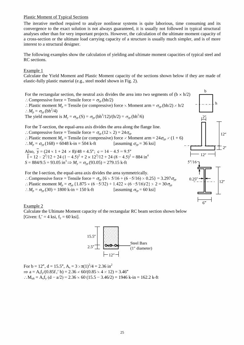
Example 1
Calculate the Yield Moment and Plastic Moment capacity of the sections shown below if they are made of
elastic-fully plastic material (e.g., steel model shown in Fig. 2).
Example 2
Calculate the Ultimate Moment capacity of the rectangular RC beam section shown below
[Given: fc = 4 ksi, fy = 60 ksi].
For b = 12 , d = 15.5 , As = 3 (1)2/4 = 2.36 in
2
a = Asfy/(0.85f c b) = 2.36 60/(0.85 4 12) = 3.46
Mult = Asfy (d − a/2) = 2.36 60 (15.5 − 3.46/2) = 1946 k-in = 162.2 k-ft
Steel Bars
(1 diameter)
12
2.5
15.5
For the rectangular section, the neutral axis divides the area into two segments of (b h/2)
Compressive force = Tensile force = yp (bh/2)
Plastic moment Mp = Tensile (or compressive) force Moment arm = yp (bh/2) h/2
Mp = yp (bh2/4)
The yield moment is My = yp (S) = yp (bh3/12)/(h/2) = yp (bh
2/6)
For the T-section, the equal-area axis divides the area along the flange line.
Compressive force = Tensile force = yp (12 2) = 24 yp
Plastic moment Mp = Tensile (or compressive) force Moment arm = 24 yp (1 + 6)
Mp = yp (168) = 6048 k-in = 504 k-ft [assuming yp = 36 ksi]
Also, y = (24 1 + 24 8)/48 = 4.5 ; c = 14 − 4.5 = 9.5
I = 12 23/12 + 24 (1 − 4.5)
2 + 2 12
3/12 + 24 (8 − 4.5)
2 = 884 in
4
S = 884/9.5 = 93.05 in3
My = yp (93.05) = 279.15 k-ft
For the I-section, the equal-area axis divides the area symmetrically.
Compressive force = Tensile force = yp {6 5/16 + (6 −5/16) 0.25} = 3.297 yp
Plastic moment Mp = yp {1.875 (6 −5/32) + 1.422 (6 −5/16)/2} 2 = 30 yp
Mp = yp (30) = 1800 k-in = 150 k-ft [assuming yp = 60 ksi]
h
2
12
12
2
b
5″/16
12
6
0.25
26
Ultimate Load of Simple Beams
Plastic Hinge and Ultimate Load
Since Plastic Moment of a section is its ultimate moment capacity, it cannot take any more moment beyond
this. As such, the section behaves almost like an internal hinge within a structure. Such a hypothetical
internal hinge is called Plastic Hinge; and by adding a new equation of statics, it reduces by one the degree
of statical indeterminacy of the structure. Therefore, formation of such hinges can make the structure
statically determinate, and eventually lead to its instability, which can cause the ultimate collapse of the
structure, at the formation of Collapse Mechanism.
By calculating the external loads necessary to form such hinges, it is possible to calculate the loads needed
to form Collapse Mechanism of the structure. This load is called the Ultimate Load of the structure and is
important to a designer because it provides information about the load that the structure can possibly sustain,
as demonstrated by the following examples.
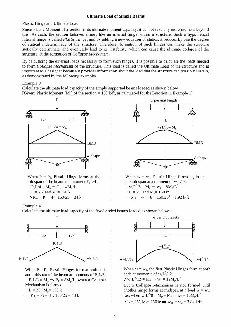
Example 3
Calculate the ultimate load capacity of the simply supported beams loaded as shown below
[Given: Plastic Moment (Mp) of the section = 150 k-ft, as calculated for the I-section in Example 1].
Example 4
Calculate the ultimate load capacity of the fixed-ended beams loaded as shown below.
P w per unit length
P1 L/4 = Mp
BMD
w1 L2/8= Mp
BMD
When P = P1, Plastic Hinge forms at the
midspan of the beam at a moment P1L/4.
P1L/4 = Mp P1 = 4Mp/L
L = 25 and Mp= 150 k
Pult = P1 = 4 150/25 = 24 k
-Shape -Shape
When w = w1, Plastic Hinge forms again at
the midspan at a moment of w1L2/8.
w1L2/8 = Mp w1 = 8Mp/L
2
L = 25 and Mp= 150 k
wult = w1 = 8 150/252 = 1.92 k/ft
P
L/2 L/2 L
w per unit length
P1 L/8
P1 L/8 P1 L/8 wL2/12 wL
2/12
When w = w1, the first Plastic Hinges form at both
ends at moments of w1L2/12.
w1L2/12 = Mp w1 = 12Mp/L
2
But a Collapse Mechanism is not formed until
another hinge forms at midspan at a load w = w2;
i.e., when w2L2/8 − Mp = Mp w2 = 16Mp/L
2
L = 25 , Mp= 150 k wult = w2 = 3.84 k/ft
When P = P1, Plastic Hinges form at both ends
and midspan of the beam at moments of P1L/8.
P1L/8 = Mp P1 = 8Mp/L, when a Collapse
Mechanism is formed
L = 25 , Mp= 150 k
Pult = P1 = 8 150/25 = 48 k
L/2 L/2 L
wL2/24
27
Energy Formulation of Collapse Mechanism
The calculation of ultimate load capacity based on bending moment diagrams demonstrates the actual
sequence of plastic hinge formulation in a structure leading to its ultimate failure. However, it requires the
bending moment diagram after each hinge formation, which may not always be convenient to form. A more
direct (though not as detailed) calculation of the ultimate load capacity is possible by using the virtual work
method on assumed collapse mechanisms of structures. As mentioned in previous formulations, if a system
in equilibrium is subjected to virtual displacements u, the virtual work done by the external forces ( WE) is
equal to the virtual work done by the internal forces ( WI); i.e., WE = WI
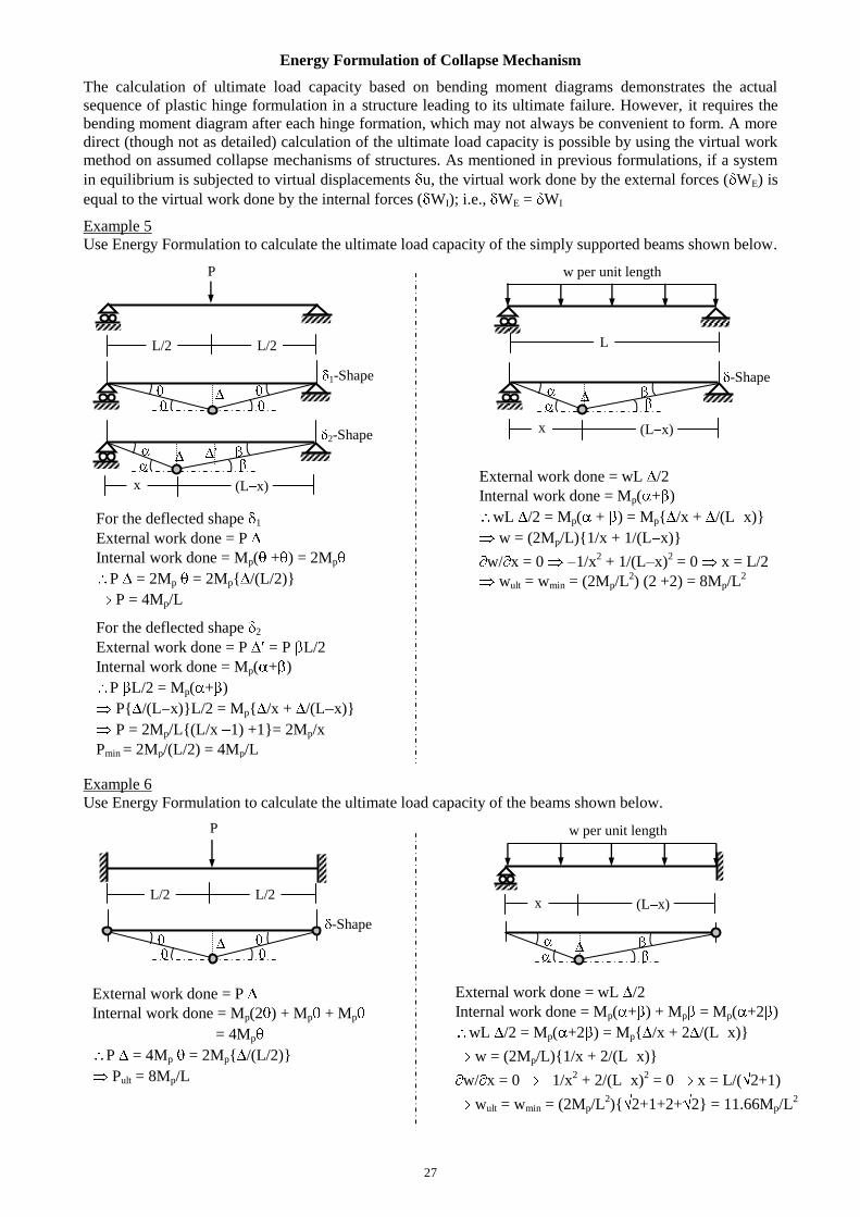
Example 5
Use Energy Formulation to calculate the ultimate load capacity of the simply supported beams shown below.
Example 6
Use Energy Formulation to calculate the ultimate load capacity of the beams shown below.
P w per unit length
For the deflected shape 1
External work done = P
Internal work done = Mp( + ) = 2Mp
P = 2Mp = 2Mp{ /(L/2)}
P = 4Mp/L
For the deflected shape 2
External work done = P = P L/2
Internal work done = Mp( + )
P L/2 = Mp( + )
P{ /(L x)}L/2 = Mp{ /x + /(L x)}
P = 2Mp/L{(L/x 1) +1}= 2Mp/x
Pmin = 2Mp/(L/2) = 4Mp/L
-Shape
External work done = wL /2
Internal work done = Mp( + )
wL /2 = Mp( + ) = Mp{ /x + /(L x)}
w = (2Mp/L){1/x + 1/(L x)}
w/ x = 0 1/x2 + 1/(L x)
2 = 0 x = L/2
wult = wmin = (2Mp/L2) (2 +2) = 8Mp/L
2
P
L/2 L/2
w per unit length
External work done = wL /2
Internal work done = Mp( + ) + Mp = Mp( +2 )
wL /2 = Mp( +2 ) = Mp{ /x + 2 /(L x)}
w = (2Mp/L){1/x + 2/(L x)}
w/ x = 0 1/x2 + 2/(L x)
2 = 0 x = L/( 2+1)
wult = wmin = (2Mp/L2){ 2+1+2+ 2} = 11.66Mp/L
2
External work done = P
Internal work done = Mp(2 ) + Mp + Mp
= 4Mp
P = 4Mp = 2Mp{ /(L/2)}
Pult = 8Mp/L
L/2 L/2 L
1-Shape
-Shape
2-Shape
x (L x)
x (L x)
x (L x)
28
Ultimate Load of Continuous Beams, Frames
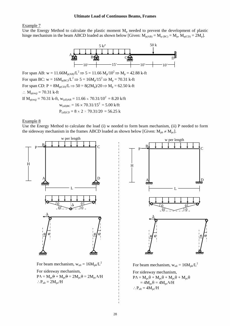
Example 7
Use the Energy Method to calculate the plastic moment Mp needed to prevent the development of plastic
hinge mechanism in the beam ABCD loaded as shown below [Given: Mp(AB) = Mp (BC) = Mp, Mp(CD) = 2Mp].
For span AB: w = 11.66Mp(AB)/L2
5 = 11.66 Mp/102
Mp = 42.88 k-ft
For span BC: w = 16Mp(BC)/L2
5 = 16Mp/152
Mp = 70.31 k-ft
For span CD: P = 8Mp(CD)/L
50 = 8(2Mp)/20
Mp = 62.50 k-ft
Mp(req) = 70.31 k-ft
If Mp(req) = 70.31 k-ft, w(all)AB = 11.66 70.31/102 = 8.20 k/ft
w(all)BC = 16 70.31/152 = 5.00 k/ft
P(all)CD = 8 2 70.31/20 = 56.25 k
Example 8
Use the Energy Method to calculate the load (i) w needed to form beam mechanism, (ii) P needed to form
the sidesway mechanism in the frames ABCD loaded as shown below [Given: Mpb Mpc].
B A
C
5 k/
D
15 10 10 10
50 k
B
A
C
w per length
L
D
P
H
B
A
C
w per length
D
P
H
L
For beam mechanism, wult = 16Mpb/L2
For sidesway mechanism,
P = Mpc + Mpc = 2Mpc = 2Mpc /H
Pult = 2Mpc/H
For beam mechanism, wult = 16Mpb/L2
For sidesway mechanism,
P = Mpc + Mpc + Mpc + Mpc
= 4Mpc = 4Mpc /H
Pult = 4Mpc/H
29
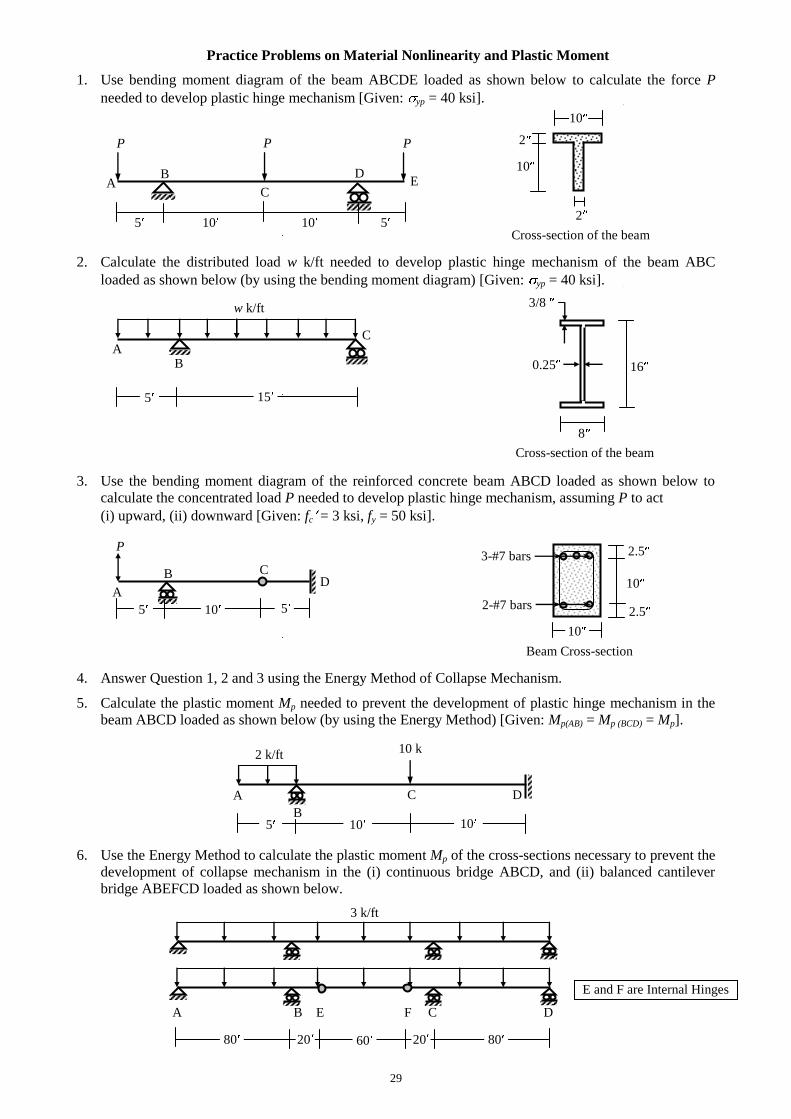
Practice Problems on Material Nonlinearity and Plastic Moment
1. Use bending moment diagram of the beam ABCDE loaded as shown below to calculate the force P
needed to develop plastic hinge mechanism [Given: yp = 40 ksi].
5 10 10 5
2. Calculate the distributed load w k/ft needed to develop plastic hinge mechanism of the beam ABC
loaded as shown below (by using the bending moment diagram) [Given: yp = 40 ksi].
3. Use the bending moment diagram of the reinforced concrete beam ABCD loaded as shown below to
calculate the concentrated load P needed to develop plastic hinge mechanism, assuming P to act
(i) upward, (ii) downward [Given: fc = 3 ksi, fy = 50 ksi].
4. Answer Question 1, 2 and 3 using the Energy Method of Collapse Mechanism.
5. Calculate the plastic moment Mp needed to prevent the development of plastic hinge mechanism in the
beam ABCD loaded as shown below (by using the Energy Method) [Given: Mp(AB) = Mp (BCD) = Mp].
6. Use the Energy Method to calculate the plastic moment Mp of the cross-sections necessary to prevent the
development of collapse mechanism in the (i) continuous bridge ABCD, and (ii) balanced cantilever
bridge ABEFCD loaded as shown below.
A B E F C D
A B
C E
P P P
D
Cross-section of the beam
Cross-section of the beam
C
3/8
16
8
0.25
A B
w k/ft
15 5
10
10
2
2
Beam Cross-section
C
A
B
10 5 5
D
P
10
10
2.5
2.5
3-#7 bars
2-#7 bars
A
2 k/ft
10 5
C
10 k
10
D
3 k/ft
E and F are Internal Hinges
80 80 60 20 20
B
30
Dynamic Equations of Motion for Lumped Mass Systems
Formulation of the Single-Degree-of-Freedom (SDOF) Equation
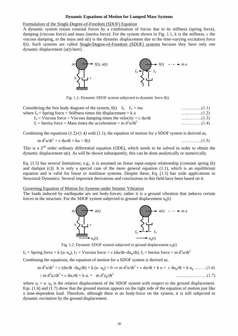
A dynamic system resists external forces by a combination of forces due to its stiffness (spring force),
damping (viscous force) and mass (inertia force). For the system shown in Fig. 1.1, k is the stiffness, c the
viscous damping, m the mass and u(t) is the dynamic displacement due to the time-varying excitation force
f(t). Such systems are called Single-Degree-of-Freedom (SDOF) systems because they have only one
dynamic displacement [u(t) here].
m f(t), u(t) f(t)
k c
Fig. 1.1: Dynamic SDOF system subjected to dynamic force f(t)
Considering the free body diagram of the system, f(t) fS fV = ma …………..(1.1)
where fS = Spring force = Stiffness times the displacement = k u …..………(1.2)
fV = Viscous force = Viscous damping times the velocity = c du/dt …..………(1.3)
fI = Inertia force = Mass times the acceleration = m d2u/dt
2 ..…………(1.4)
Combining the equations (1.2)-(1.4) with (1.1), the equation of motion for a SDOF system is derived as,
m d2u/dt
2 + c du/dt + ku = f(t) …..………(1.5)
This is a 2nd
order ordinary differential equation (ODE), which needs to be solved in order to obtain the
dynamic displacement u(t). As will be shown subsequently, this can be done analytically or numerically.
Eq. (1.5) has several limitations; e.g., it is assumed on linear input-output relationship [constant spring (k)
and dashpot (c)]. It is only a special case of the more general equation (1.1), which is an equilibrium
equation and is valid for linear or nonlinear systems. Despite these, Eq. (1.5) has wide applications in
Structural Dynamics. Several important derivations and conclusions in this field have been based on it.
Governing Equation of Motion for Systems under Seismic Vibration
The loads induced by earthquake are not body-forces; rather it is a ground vibration that induces certain
forces in the structure. For the SDOF system subjected to ground displacement ug(t)
m u(t) u(t)
k c
Fig. 1.2: Dynamic SDOF system subjected to ground displacement ug(t)
fS = Spring force = k (u ug), fV = Viscous force = c (du/dt dug/dt), fI = Inertia force = m d2u/dt
2
Combining the equations, the equation of motion for a SDOF system is derived as,
m d2u/dt
2 + c (du/dt dug/dt) + k (u ug) = 0 m d
2u/dt
2 + c du/dt + k u = c dug/dt + k ug ...……(1.6)
m d2ur/dt
2 + c dur/dt + k ur = m d
2ug/dt
2 ..…..……………(1.7)
where ur = u ug is the relative displacement of the SDOF system with respect to the ground displacement.
Eqs. (1.6) and (1.7) show that the ground motion appears on the right side of the equation of motion just like
a time-dependent load. Therefore, although there is no body-force on the system, it is still subjected to
dynamic excitation by the ground displacement.
fS fV
m a
fS fV
m a
ug(t) ug(t)
31
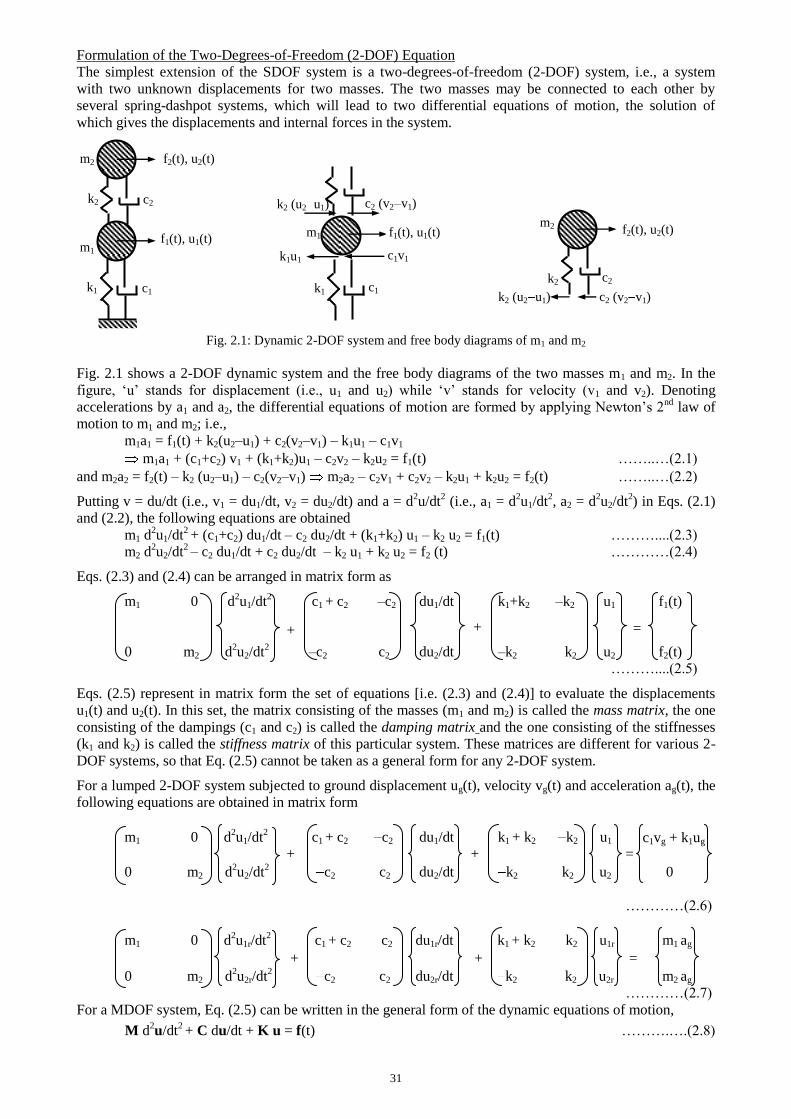
Formulation of the Two-Degrees-of-Freedom (2-DOF) Equation
The simplest extension of the SDOF system is a two-degrees-of-freedom (2-DOF) system, i.e., a system
with two unknown displacements for two masses. The two masses may be connected to each other by
several spring-dashpot systems, which will lead to two differential equations of motion, the solution of
which gives the displacements and internal forces in the system.
Fig. 2.1: Dynamic 2-DOF system and free body diagrams of m1 and m2
Fig. 2.1 shows a 2-DOF dynamic system and the free body diagrams of the two masses m1 and m2. In the
figure, ‘u’ stands for displacement (i.e., u1 and u2) while ‘v’ stands for velocity (v1 and v2). Denoting
accelerations by a1 and a2, the differential equations of motion are formed by applying Newton’s 2nd
law of
motion to m1 and m2; i.e.,
m1a1 = f1(t) + k2(u2–u1) + c2(v2–v1) – k1u1 – c1v1
m1a1 + (c1+c2) v1 + (k1+k2)u1 – c2v2 – k2u2 = f1(t) ……..…(2.1)
and m2a2 = f2(t) – k2 (u2–u1) – c2(v2–v1) m2a2 – c2v1 + c2v2 – k2u1 + k2u2 = f2(t) ……..…(2.2)
Putting v = du/dt (i.e., v1 = du1/dt, v2 = du2/dt) and a = d2u/dt
2 (i.e., a1 = d
2u1/dt
2, a2 = d
2u2/dt
2) in Eqs. (2.1)
and (2.2), the following equations are obtained
m1 d2u1/dt
2 + (c1+c2) du1/dt – c2 du2/dt + (k1+k2) u1 – k2 u2 = f1(t) ………....(2.3)
m2 d2u2/dt
2 – c2 du1/dt + c2 du2/dt – k2 u1 + k2 u2 = f2 (t) …………(2.4)
Eqs. (2.3) and (2.4) can be arranged in matrix form as
m1 0 d2u1/dt
2 c1 + c2 –c2 du1/dt k1+k2 –k2 u1 f1(t)
0 m2 d2u2/dt
2 –c2 c2 du2/dt –k2 k2 u2 f2(t)
………....(2.5)
Eqs. (2.5) represent in matrix form the set of equations [i.e. (2.3) and (2.4)] to evaluate the displacements
u1(t) and u2(t). In this set, the matrix consisting of the masses (m1 and m2) is called the mass matrix, the one
consisting of the dampings (c1 and c2) is called the damping matrix and the one consisting of the stiffnesses
(k1 and k2) is called the stiffness matrix of this particular system. These matrices are different for various 2-
DOF systems, so that Eq. (2.5) cannot be taken as a general form for any 2-DOF system.
For a lumped 2-DOF system subjected to ground displacement ug(t), velocity vg(t) and acceleration ag(t), the
following equations are obtained in matrix form
m1 0 d2u1/dt
2 c1 + c2 c2 du1/dt k1 + k2 k2 u1
+ + =
0 m2 d2u2/dt
2 c2 c2 du2/dt k2 k2 u2 0
…………(2.6)
m1 0 d2u1r/dt
2 c1 + c2 c2 du1r/dt k1 + k2 k2 u1r m1 ag
+ + =
0 m2 d2u2r/dt
2 c2 c2 du2r/dt k2 k2 u2r m2 ag
…………(2.7)
For a MDOF system, Eq. (2.5) can be written in the general form of the dynamic equations of motion,
M d2u/dt
2 + C du/dt + K u = f(t) ……….….(2.8)
c1 k1
m1
c1v1
c2 (v2 v1) k2 (u2 u1)
c2 (v2 v1) k2 (u2 u1)
c2
f2(t), u2(t)
c1
f1(t), u1(t)
k2
m2
k1
m1 k1u1
f2(t), u2(t)
c2 k2
m2
+ + =
f1(t), u1(t)
c1vg + k1ug

32
Numerical Solution of SDOF Equation
The equation of motion for a SDOF system can be solved analytically for different loading functions. Even
if the assumptions of linear structural properties are satisfied; the practical loading situations can be more
complicated and not convenient to solve analytically. Numerical methods must be used in such situations.
The most widely used numerical approach for solving dynamic problems is the Newmark- method.
Actually, it is a set of solution methods with different physical interpretations for different values of . The
total simulation time is divided into a number of intervals (usually of equal duration t) and the unknown
displacement (as well as velocity and acceleration) is solved at each instant of time. The method solves the
dynamic equation of motion in the (i + 1)th time step based on the results of the i
th step.
The equation of motion for the (i +1)th time step is
m (d2u/dt
2)i+1 + c (du/dt)i+1 + k (u)i+1 = f i+1 m ai+1 + c vi+1 + k ui+1 = f i+1 …..………(3.1)
where ‘a’ stands for the acceleration, ‘v’ for velocity and ‘u’ for displacement.
To solve for the displacement or acceleration at the (i + 1)th time step, the following equations are assumed
for the velocity and displacement at the (i + 1)th step in terms of the values at the i
th step.
vi+1 = vi + {(1 ) ai + ai+1} t ….…………(3.2)
ui+1 = ui + vi t + {(0.5 ) ai + ai+1} t2 …….………(3.3)
By putting the value of vi+1 from Eq. (3.2) and ui+1 from Eq. (3.3) in Eq. (3.1), the only unknown variable ai+1
can be solved from Eq. (3.1).
In the solution set suggested by the Newmark- method, the Constant Average Acceleration (CAA) method
is the most popular because of the stability of its solutions and the simple physical interpretations it
provides. This method assumes the acceleration to remain constant during each small time interval t, and
this constant is assumed to be the average of the accelerations at the two instants of time ti and ti+1. The CAA
is a special case of Newmark- method where = 0.50 and = 0.25. Thus in the CAA method, the
equations for velocity and displacement [Eqs. (3.2) and (3.3)] become
vi+1 = vi + (ai + ai+1) t/2 ……………(3.4)
ui+1 = ui + vi t + (ai + ai+1) t2/4 ……………(3.5)
Inserting these values in Eq. (3.1) and rearranging the coefficients, the following equation is obtained,
(m + c t /2 + k t2/4)ai+1 = fi+1 – kui – (c + k t)vi – (c t/2 + k t
2/4)ai ….….…..(3.6)
(meff) ai+1 = fi+1 – kui –(ceff) vi – (meff1) ai ….….…..(3.6)
To obtain the acceleration ai+1 at an instant of time ti+1 using Eq. (3.6), the values of ui, vi and ai at the
previous instant ti have to be known (or calculated) before. Once ai+1 is obtained, Eqs. (3.4) and (3.5) can be
used to calculate the velocity vi+1 and displacement ui+1 at time ti+1. All these values can be used to obtain the
results at time ti+2. The method can be used for subsequent time-steps also.
The simulation should start with two initial conditions, like the displacement u0 and velocity v0 at time t0 = 0.
The initial acceleration can be obtained from the equation of motion at time t0 = 0 as
a0 = (f0 – cv0 – ku0)/m ……………(3.7)
33
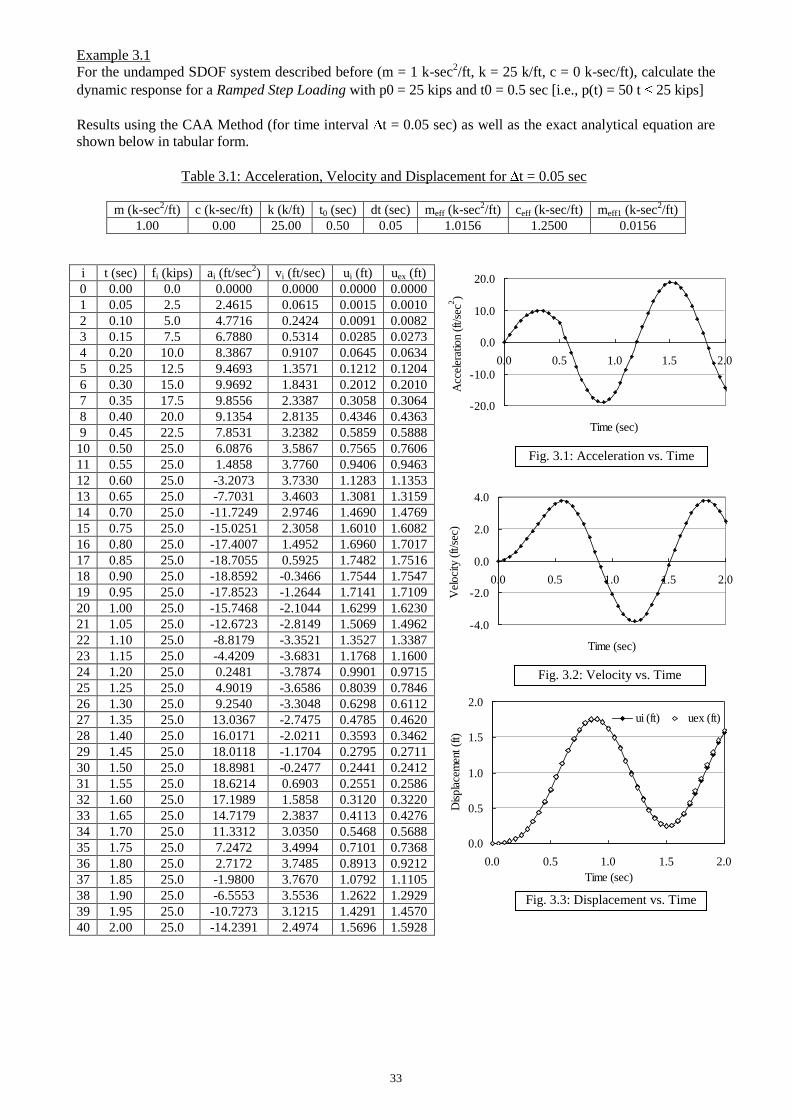
Example 3.1
For the undamped SDOF system described before (m = 1 k-sec2/ft, k = 25 k/ft, c = 0 k-sec/ft), calculate the
dynamic response for a Ramped Step Loading with p0 = 25 kips and t0 = 0.5 sec [i.e., p(t) = 50 t 25 kips]
Results using the CAA Method (for time interval t = 0.05 sec) as well as the exact analytical equation are
shown below in tabular form.
Table 3.1: Acceleration, Velocity and Displacement for t = 0.05 sec
m (k-sec2/ft) c (k-sec/ft) k (k/ft) t0 (sec) dt (sec) meff (k-sec
2/ft) ceff (k-sec/ft) meff1 (k-sec
2/ft)
1.00 0.00 25.00 0.50 0.05 1.0156 1.2500 0.0156
i t (sec) fi (kips) ai (ft/sec2) vi (ft/sec) ui (ft) uex (ft)
0 0.00 0.0 0.0000 0.0000 0.0000 0.0000
1 0.05 2.5 2.4615 0.0615 0.0015 0.0010
2 0.10 5.0 4.7716 0.2424 0.0091 0.0082
3 0.15 7.5 6.7880 0.5314 0.0285 0.0273
4 0.20 10.0 8.3867 0.9107 0.0645 0.0634
5 0.25 12.5 9.4693 1.3571 0.1212 0.1204
6 0.30 15.0 9.9692 1.8431 0.2012 0.2010
7 0.35 17.5 9.8556 2.3387 0.3058 0.3064
8 0.40 20.0 9.1354 2.8135 0.4346 0.4363
9 0.45 22.5 7.8531 3.2382 0.5859 0.5888
10 0.50 25.0 6.0876 3.5867 0.7565 0.7606
11 0.55 25.0 1.4858 3.7760 0.9406 0.9463
12 0.60 25.0 -3.2073 3.7330 1.1283 1.1353
13 0.65 25.0 -7.7031 3.4603 1.3081 1.3159
14 0.70 25.0 -11.7249 2.9746 1.4690 1.4769
15 0.75 25.0 -15.0251 2.3058 1.6010 1.6082
16 0.80 25.0 -17.4007 1.4952 1.6960 1.7017
17 0.85 25.0 -18.7055 0.5925 1.7482 1.7516
18 0.90 25.0 -18.8592 -0.3466 1.7544 1.7547
19 0.95 25.0 -17.8523 -1.2644 1.7141 1.7109
20 1.00 25.0 -15.7468 -2.1044 1.6299 1.6230
21 1.05 25.0 -12.6723 -2.8149 1.5069 1.4962
22 1.10 25.0 -8.8179 -3.3521 1.3527 1.3387
23 1.15 25.0 -4.4209 -3.6831 1.1768 1.1600
24 1.20 25.0 0.2481 -3.7874 0.9901 0.9715
25 1.25 25.0 4.9019 -3.6586 0.8039 0.7846
26 1.30 25.0 9.2540 -3.3048 0.6298 0.6112
27 1.35 25.0 13.0367 -2.7475 0.4785 0.4620
28 1.40 25.0 16.0171 -2.0211 0.3593 0.3462
29 1.45 25.0 18.0118 -1.1704 0.2795 0.2711
30 1.50 25.0 18.8981 -0.2477 0.2441 0.2412
31 1.55 25.0 18.6214 0.6903 0.2551 0.2586
32 1.60 25.0 17.1989 1.5858 0.3120 0.3220
33 1.65 25.0 14.7179 2.3837 0.4113 0.4276
34 1.70 25.0 11.3312 3.0350 0.5468 0.5688
35 1.75 25.0 7.2472 3.4994 0.7101 0.7368
36 1.80 25.0 2.7172 3.7485 0.8913 0.9212
37 1.85 25.0 -1.9800 3.7670 1.0792 1.1105
38 1.90 25.0 -6.5553 3.5536 1.2622 1.2929
39 1.95 25.0 -10.7273 3.1215 1.4291 1.4570
40 2.00 25.0 -14.2391 2.4974 1.5696 1.5928
Fig. 6.1: Acceleration vs. Time
-20.0
-10.0
0.0
10.0
20.0
0.0 0.5 1.0 1.5 2.0
Time (sec)
Acc
eler
atio
n (f
t/se
c2)
Fig. 6.2: Velocity vs. Time
-4.0
-2.0
0.0
2.0
4.0
0.0 0.5 1.0 1.5 2.0
Time (sec)
Vel
oci
ty (
ft/s
ec)
Fig. 6.3: Displacement vs. Time
0.0
0.5
1.0
1.5
2.0
0.0 0.5 1.0 1.5 2.0
Time (sec)
Dis
pla
cem
ent (f
t)
ui (ft) uex (ft)
Fig. 3.1: Acceleration vs. Time
Fig. 3.2: Velocity vs. Time
Fig. 3.3: Displacement vs. Time
34
Stiffness and Mass Matrices of Continuous Systems
Axial Members
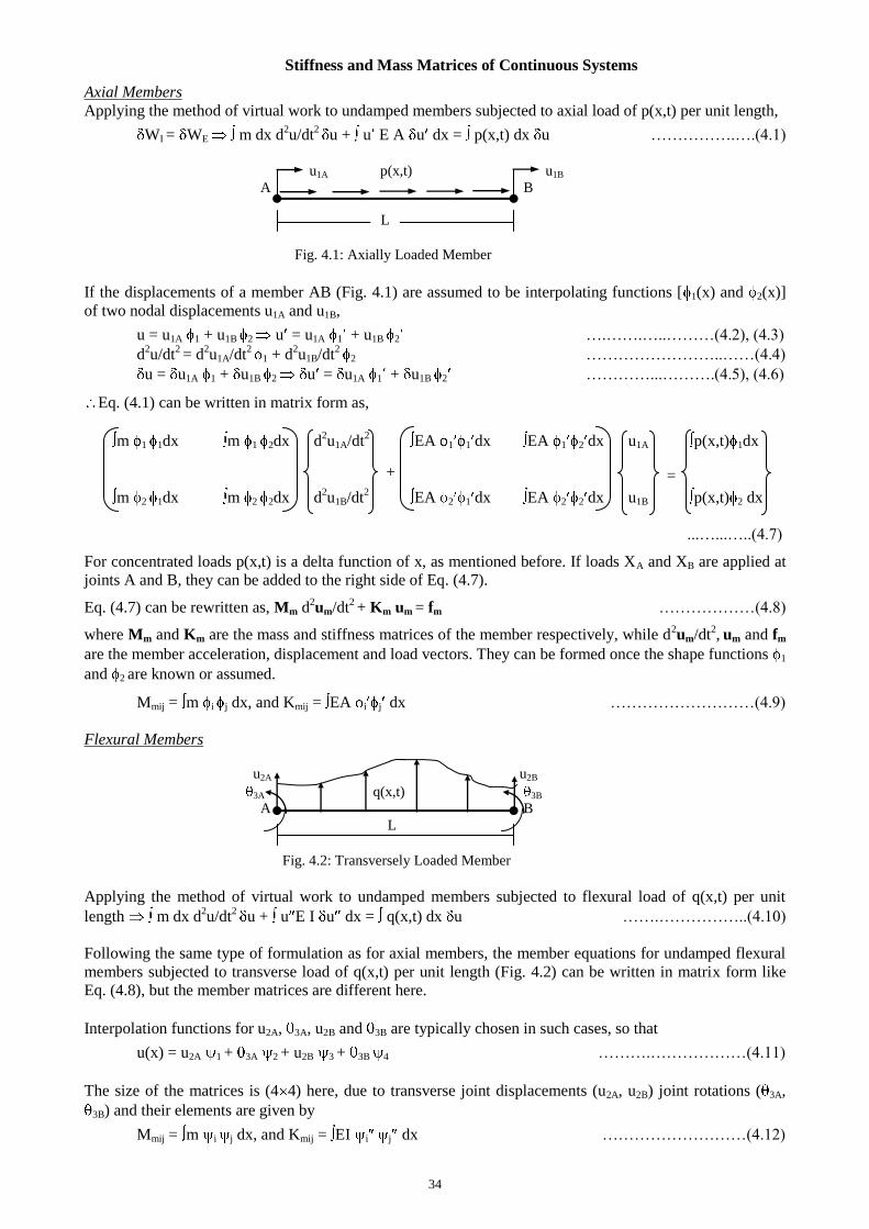
Applying the method of virtual work to undamped members subjected to axial load of p(x,t) per unit length,
WI = WE m dx d2u/dt
2 u + u E A u dx = p(x,t) dx u …………….….(4.1)
u1A p(x,t) u1B
A B
Fig. 4.1: Axially Loaded Member
If the displacements of a member AB (Fig. 4.1) are assumed to be interpolating functions [ 1(x) and 2(x)]
of two nodal displacements u1A and u1B,
u = u1A 1 + u1B 2 u = u1A 1 + u1B 2 ….…….…..………(4.2), (4.3)
d2u/dt
2 = d
2u1A/dt
2 1 + d
2u1B/dt
2 2 ……………………..……(4.4)
u = u1A 1 + u1B 2 u = u1A 1 + u1B 2 …………...……….(4.5), (4.6)
Eq. (4.1) can be written in matrix form as,
m 1 1dx m 1
2dx d2u1A/dt
2 EA 1 1 dx EA 1 2 dx u1A p(x,t) 1dx
m 2 1dx m 2
2dx d2u1B/dt
2 EA 2 1 dx EA 2 2 dx u1B p(x,t) 2 dx
...…...…..(4.7)
For concentrated loads p(x,t) is a delta function of x, as mentioned before. If loads XA and XB are applied at
joints A and B, they can be added to the right side of Eq. (4.7).
Eq. (4.7) can be rewritten as, Mm d2um/dt
2 + Km um
= fm ………………(4.8)
where Mm and Km are the mass and stiffness matrices of the member respectively, while d2um/dt
2, um and fm
are the member acceleration, displacement and load vectors. They can be formed once the shape functions 1
and 2 are known or assumed.
Mmij = m i
j dx, and Kmij = EA i j dx ………………………(4.9)
Flexural Members
u2A u2B
3A q(x,t) 3B
A B
L
Fig. 4.2: Transversely Loaded Member
Applying the method of virtual work to undamped members subjected to flexural load of q(x,t) per unit
length m dx d2u/dt
2 u + u E I u dx = q(x,t) dx u …….……………..(4.10)
Following the same type of formulation as for axial members, the member equations for undamped flexural
members subjected to transverse load of q(x,t) per unit length (Fig. 4.2) can be written in matrix form like
Eq. (4.8), but the member matrices are different here.
Interpolation functions for u2A, 3A, u2B and 3B are typically chosen in such cases, so that
u(x) = u2A 1 + 3A 2 + u2B 3 + 3B 4 ……….………………(4.11)
The size of the matrices is (4 4) here, due to transverse joint displacements (u2A, u2B) joint rotations ( 3A,
3B) and their elements are given by
Mmij = m i
j dx, and Kmij = EI i
j dx ………………………(4.12)
+ =
L
35
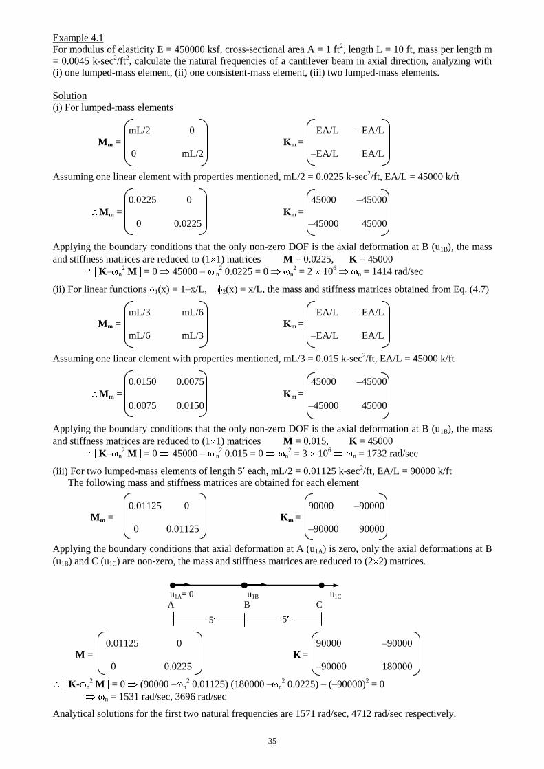
Example 4.1
For modulus of elasticity E = 450000 ksf, cross-sectional area A = 1 ft2, length L = 10 ft, mass per length m
= 0.0045 k-sec2/ft
2, calculate the natural frequencies of a cantilever beam in axial direction, analyzing with
(i) one lumped-mass element, (ii) one consistent-mass element, (iii) two lumped-mass elements.
Solution
(i) For lumped-mass elements
mL/2 0 EA/L –EA/L
Mm = Km =
0 mL/2 –EA/L EA/L
Assuming one linear element with properties mentioned, mL/2 = 0.0225 k-sec2/ft, EA/L = 45000 k/ft
0.0225 0 45000 –45000
Mm = Km =
0 0.0225 –45000 45000
Applying the boundary conditions that the only non-zero DOF is the axial deformation at B (u1B), the mass
and stiffness matrices are reduced to (1 1) matrices M = 0.0225, K = 45000
K– n2 M = 0 45000 – n
2 0.0225 = 0 n
2 = 2 10
6 n = 1414 rad/sec
(ii) For linear functions 1(x) = 1–x/L, 2(x) = x/L, the mass and stiffness matrices obtained from Eq. (4.7)
mL/3 mL/6 EA/L –EA/L
Mm = Km =
mL/6 mL/3 –EA/L EA/L
Assuming one linear element with properties mentioned, mL/3 = 0.015 k-sec2/ft, EA/L = 45000 k/ft
0.0150 0.0075 45000 –45000
Mm = Km =
0.0075 0.0150 –45000 45000
Applying the boundary conditions that the only non-zero DOF is the axial deformation at B (u1B), the mass
and stiffness matrices are reduced to (1 1) matrices M = 0.015, K = 45000
K– n2 M = 0 45000 – n
2 0.015 = 0 n
2 = 3 10
6 n = 1732 rad/sec
(iii) For two lumped-mass elements of length 5 each, mL/2 = 0.01125 k-sec2/ft, EA/L = 90000 k/ft
The following mass and stiffness matrices are obtained for each element
0.01125 0 90000 –90000
Mm = Km =
0 0.01125 –90000 90000
Applying the boundary conditions that axial deformation at A (u1A) is zero, only the axial deformations at B
(u1B) and C (u1C) are non-zero, the mass and stiffness matrices are reduced to (2 2) matrices.
u1A= 0 u1B u1C
A B C
0.01125 0 90000 –90000
M = K =
0 0.0225 –90000 180000
K- n2 M = 0 (90000 – n
2 0.01125) (180000 – n
2 0.0225) – (–90000)
2 = 0
n = 1531 rad/sec, 3696 rad/sec
Analytical solutions for the first two natural frequencies are 1571 rad/sec, 4712 rad/sec respectively.
5 5
36
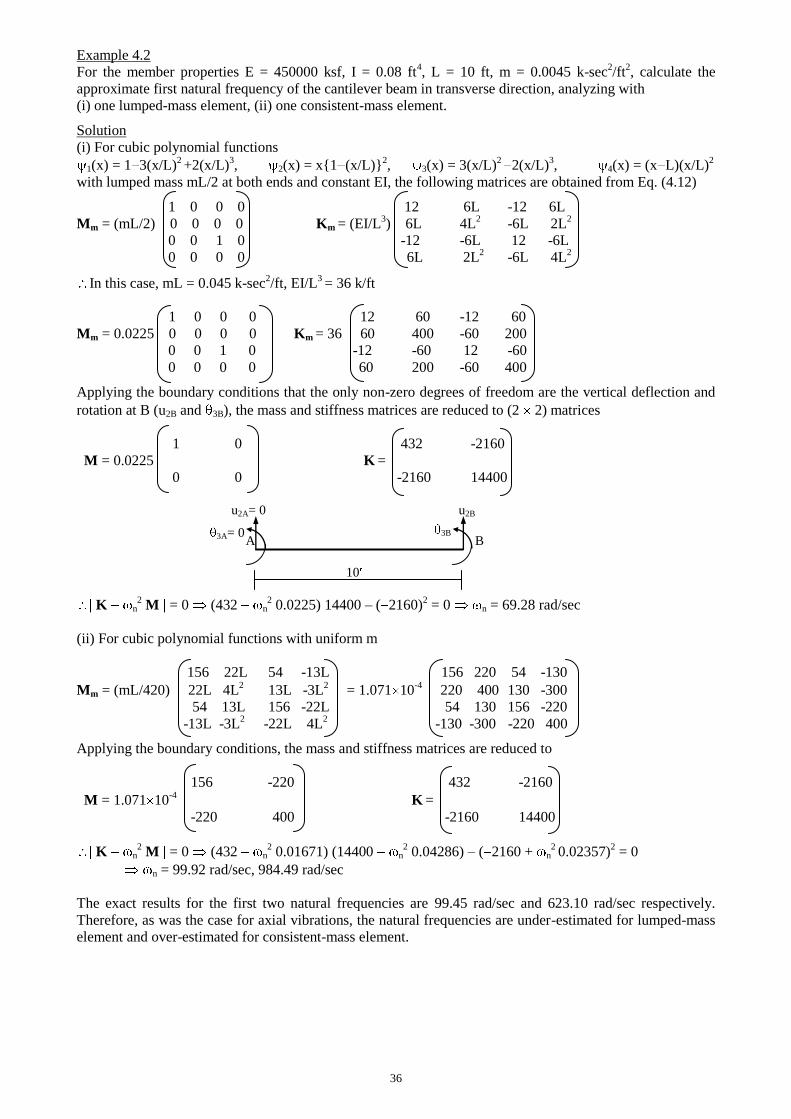
Example 4.2
For the member properties E = 450000 ksf, I = 0.08 ft4, L = 10 ft, m = 0.0045 k-sec
2/ft
2, calculate the
approximate first natural frequency of the cantilever beam in transverse direction, analyzing with
(i) one lumped-mass element, (ii) one consistent-mass element.
Solution
(i) For cubic polynomial functions
1(x) = 1 3(x/L)2 +2(x/L)
3, 2(x) = x{1 (x/L)}
2, 3(x) = 3(x/L)
2 2(x/L)
3, 4(x) = (x L)(x/L)
2
with lumped mass mL/2 at both ends and constant EI, the following matrices are obtained from Eq. (4.12)
1 0 0 0 12 6L -12 6L
Mm = (mL/2) 0 0 0 0 Km = (EI/L3) 6L 4L
2 -6L 2L
2
0 0 1 0 -12 -6L 12 -6L
0 0 0 0
6L 2L2 -6L 4L
2
In this case, mL = 0.045 k-sec2/ft, EI/L
3 = 36 k/ft
1 0 0 0 12 60 -12 60
Mm = 0.0225 0 0 0 0 Km = 36 60 400 -60 200
0 0 1 0 -12 -60 12 -60
0 0 0 0
60 200 -60 400
Applying the boundary conditions that the only non-zero degrees of freedom are the vertical deflection and
rotation at B (u2B and 3B), the mass and stiffness matrices are reduced to (2 2) matrices
1 0 432 -2160
M = 0.0225 K =
0 0 -2160 14400
u2A= 0 u2B
A B
10
K n2 M = 0 (432 n
2 0.0225) 14400 – ( 2160)
2 = 0 n = 69.28 rad/sec
(ii) For cubic polynomial functions with uniform m
156 22L 54 -13L 156 220 54 -130
Mm = (mL/420) 22L 4L2 13L -3L
2 = 1.071 10
-4 220 400 130 -300
54 13L 156 -22L 54 130 156 -220
-13L -3L2
-22L 4L2
-130 -300
-220 400
Applying the boundary conditions, the mass and stiffness matrices are reduced to
156 -220 432 -2160
M = 1.071 10-4
K =
-220 400 -2160 14400
K n2 M = 0 (432 n
2 0.01671) (14400 n
2 0.04286) – ( 2160 + n
2 0.02357)
2 = 0
n = 99.92 rad/sec, 984.49 rad/sec
The exact results for the first two natural frequencies are 99.45 rad/sec and 623.10 rad/sec respectively.
Therefore, as was the case for axial vibrations, the natural frequencies are under-estimated for lumped-mass
element and over-estimated for consistent-mass element.
3A= 0 3B
37
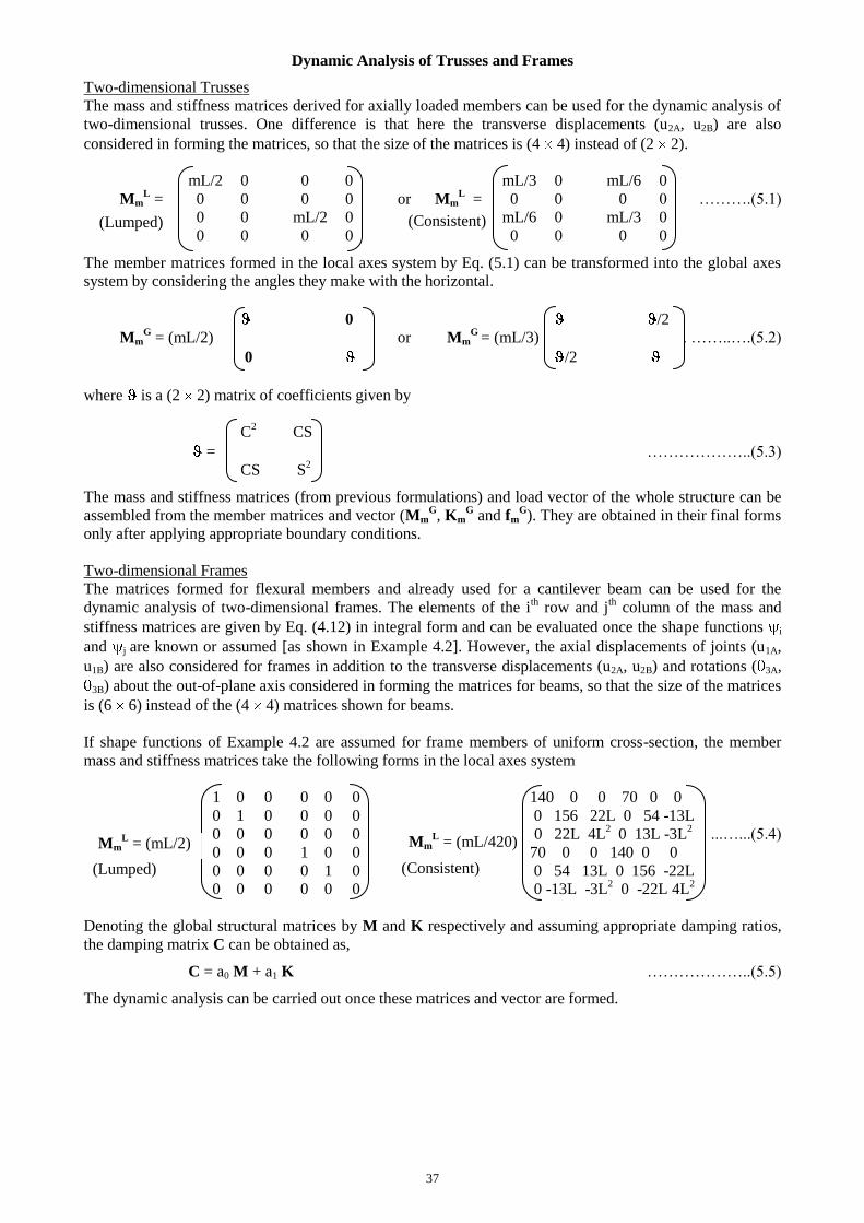
Dynamic Analysis of Trusses and Frames
Two-dimensional Trusses
The mass and stiffness matrices derived for axially loaded members can be used for the dynamic analysis of
two-dimensional trusses. One difference is that here the transverse displacements (u2A, u2B) are also
considered in forming the matrices, so that the size of the matrices is (4 4) instead of (2 2).
mL/2 0 0 0 mL/3 0 mL/6 0
MmL = 0 0 0 0 or Mm
L = 0 0 0 0 ……….(5.1)
0 0 mL/2 0 mL/6 0 mL/3 0
0 0 0 0 0 0 0 0
The member matrices formed in the local axes system by Eq. (5.1) can be transformed into the global axes
system by considering the angles they make with the horizontal.
0 /2
MmG = (mL/2) or Mm
G = (mL/3) . ……..….(5.2)
0 /2
where is a (2 2) matrix of coefficients given by
C2 CS
= ………………..(5.3)
CS S2
The mass and stiffness matrices (from previous formulations) and load vector of the whole structure can be
assembled from the member matrices and vector (MmG, Km
G and fm
G). They are obtained in their final forms
only after applying appropriate boundary conditions.
Two-dimensional Frames
The matrices formed for flexural members and already used for a cantilever beam can be used for the
dynamic analysis of two-dimensional frames. The elements of the ith row and j
th column of the mass and
stiffness matrices are given by Eq. (4.12) in integral form and can be evaluated once the shape functions i
and j are known or assumed [as shown in Example 4.2]. However, the axial displacements of joints (u1A,
u1B) are also considered for frames in addition to the transverse displacements (u2A, u2B) and rotations ( 3A,
3B) about the out-of-plane axis considered in forming the matrices for beams, so that the size of the matrices
is (6 6) instead of the (4 4) matrices shown for beams.
If shape functions of Example 4.2 are assumed for frame members of uniform cross-section, the member
mass and stiffness matrices take the following forms in the local axes system
1 0 0 0 0 0 140 0 0 70 0 0
0 1 0 0 0 0 0 156 22L 0 54 -13L
0 0 0 0 0 0 0 22L 4L2
0 13L -3L2
...…...(5.4)
0 0 0 1 0 0 70 0 0 140 0 0
0 0 0 0 1 0 0 54 13L 0 156 -22L
0 0 0 0 0 0 0 -13L -3L2 0 -22L 4L
2
Denoting the global structural matrices by M and K respectively and assuming appropriate damping ratios,
the damping matrix C can be obtained as,
C = a0 M + a1 K ………………..(5.5)
The dynamic analysis can be carried out once these matrices and vector are formed.
MmL = (mL/2)
(Lumped) (Consistent)
MmL = (mL/420)
(Lumped) (Consistent)
38
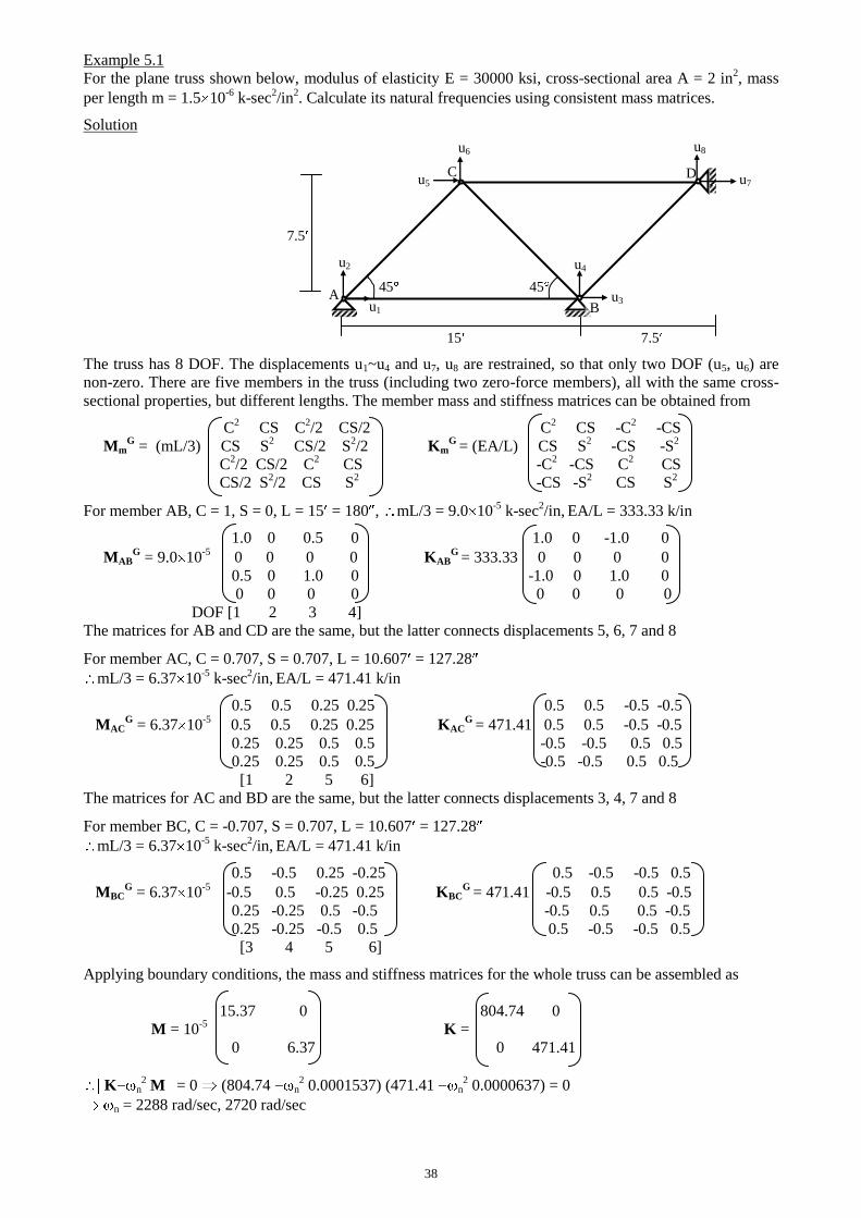
Example 5.1
For the plane truss shown below, modulus of elasticity E = 30000 ksi, cross-sectional area A = 2 in2, mass
per length m = 1.5 10-6
k-sec2/in
2. Calculate its natural frequencies using consistent mass matrices.
Solution
7.5
45 45
15 7.5
The truss has 8 DOF. The displacements u1~u4 and u7, u8 are restrained, so that only two DOF (u5, u6) are
non-zero. There are five members in the truss (including two zero-force members), all with the same cross-
sectional properties, but different lengths. The member mass and stiffness matrices can be obtained from
C2 CS C
2/2 CS/2 C
2 CS -C
2 -CS
MmG = (mL/3) CS S
2 CS/2 S
2/2 Km
G = (EA/L) CS S
2 -CS -S
2
C2/2 CS/2 C
2 CS -C
2 -CS C
2 CS
CS/2 S2/2 CS S
2 -CS -S
2 CS S
2
For member AB, C = 1, S = 0, L = 15 = 180 , mL/3 = 9.0 10-5
k-sec2/in,
EA/L = 333.33 k/in
1.0 0 0.5 0 1.0 0 -1.0 0
MABG = 9.0 10
-5 0 0 0 0 KAB
G = 333.33 0 0 0 0
0.5 0 1.0 0 -1.0 0 1.0 0
0 0 0 0
0 0 0 0
DOF [1 2 3 4]
The matrices for AB and CD are the same, but the latter connects displacements 5, 6, 7 and 8
For member AC, C = 0.707, S = 0.707, L = 10.607 = 127.28
mL/3 = 6.37 10-5
k-sec2/in,
EA/L = 471.41 k/in
0.5 0.5 0.25 0.25 0.5 0.5 -0.5 -0.5
MACG = 6.37 10
-5 0.5 0.5 0.25 0.25 KAC
G = 471.41 0.5 0.5 -0.5 -0.5
0.25 0.25 0.5 0.5 -0.5 -0.5 0.5 0.5
0.25 0.25 0.5 0.5
-0.5 -0.5 0.5 0.5
[1 2 5 6]
The matrices for AC and BD are the same, but the latter connects displacements 3, 4, 7 and 8
For member BC, C = -0.707, S = 0.707, L = 10.607 = 127.28
mL/3 = 6.37 10-5
k-sec2/in,
EA/L = 471.41 k/in
0.5 -0.5 0.25 -0.25 0.5 -0.5 -0.5 0.5
MBCG = 6.37 10
-5 -0.5 0.5 -0.25 0.25 KBC
G = 471.41 -0.5 0.5 0.5 -0.5
0.25 -0.25 0.5 -0.5 -0.5 0.5 0.5 -0.5
0.25 -0.25 -0.5 0.5
0.5 -0.5 -0.5 0.5
[3 4 5 6]
Applying boundary conditions, the mass and stiffness matrices for the whole truss can be assembled as
15.37 0 804.74 0
M = 10-5
K =
0 6.37 0 471.41
K n2 M = 0 (804.74 n
2 0.0001537) (471.41 n
2 0.0000637) = 0
n = 2288 rad/sec, 2720 rad/sec
C D
A
u8
u2
u1
u4
u3
u7
u6
u5
B
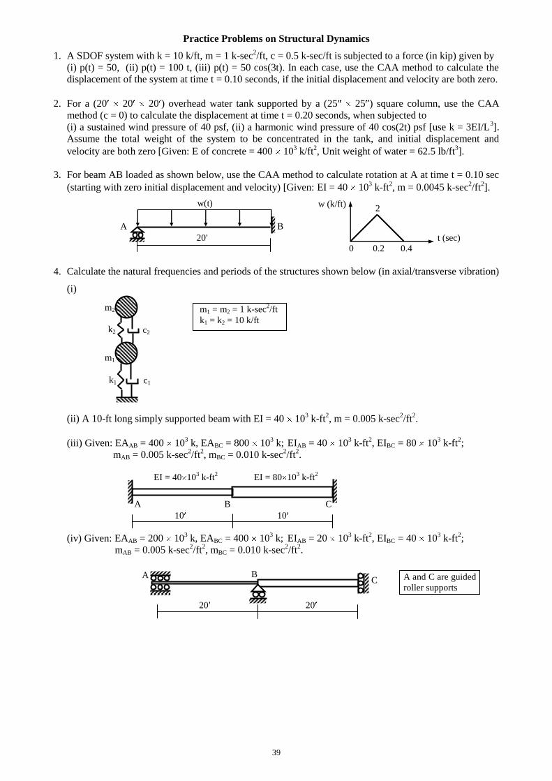
39
Practice Problems on Structural Dynamics
1. A SDOF system with k = 10 k/ft, m = 1 k-sec2/ft, c = 0.5 k-sec/ft is subjected to a force (in kip) given by
(i) p(t) = 50, (ii) p(t) = 100 t, (iii) p(t) = 50 cos(3t). In each case, use the CAA method to calculate the
displacement of the system at time t = 0.10 seconds, if the initial displacement and velocity are both zero.
2. For a (20 20 20 ) overhead water tank supported by a (25 25 ) square column, use the CAA
method (c = 0) to calculate the displacement at time t = 0.20 seconds, when subjected to
(i) a sustained wind pressure of 40 psf, (ii) a harmonic wind pressure of 40 cos(2t) psf [use k = 3EI/L3].
Assume the total weight of the system to be concentrated in the tank, and initial displacement and
velocity are both zero [Given: E of concrete = 400 103 k/ft
2, Unit weight of water = 62.5 lb/ft
3].
3. For beam AB loaded as shown below, use the CAA method to calculate rotation at A at time t = 0.10 sec
(starting with zero initial displacement and velocity) [Given: EI = 40 103 k-ft
2, m = 0.0045 k-sec
2/ft
2].
w (k/ft)
A B
20 t (sec) 0 0.2 0.4
4. Calculate the natural frequencies and periods of the structures shown below (in axial/transverse vibration)
(i)
(ii) A 10-ft long simply supported beam with EI = 40 103 k-ft
2, m = 0.005 k-sec
2/ft
2.
(iii) Given: EAAB = 400 103 k, EABC = 800 10
3 k; EIAB = 40 10
3 k-ft
2, EIBC = 80 10
3 k-ft
2;
mAB = 0.005 k-sec2/ft
2, mBC = 0.010 k-sec
2/ft
2.
EI = 40 103 k-ft
2 EI = 80 10
3 k-ft
2
A B C
10 10
(iv) Given: EAAB = 200 103 k, EABC = 400 10
3 k; EIAB = 20 10
3 k-ft
2, EIBC = 40 10
3 k-ft
2;
mAB = 0.005 k-sec2/ft
2, mBC = 0.010 k-sec
2/ft
2.
20 20
C A A and C are guided
roller supports
w(t)
m2 m1 = m2 = 1 k-sec2/ft
k1 = k2 = 10 k/ft k2
k1
m1
c2
c1
B
2
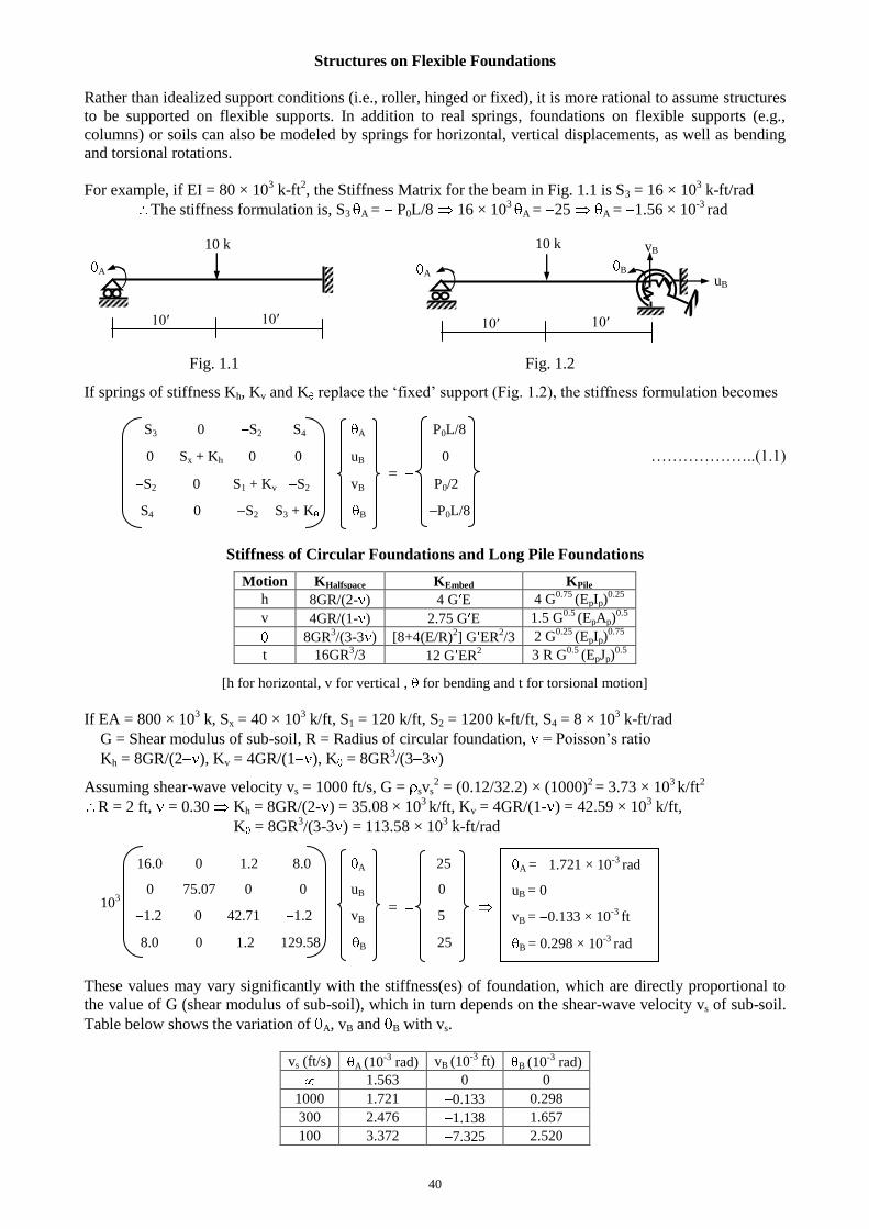
40
Structures on Flexible Foundations
Rather than idealized support conditions (i.e., roller, hinged or fixed), it is more rational to assume structures
to be supported on flexible supports. In addition to real springs, foundations on flexible supports (e.g.,
columns) or soils can also be modeled by springs for horizontal, vertical displacements, as well as bending
and torsional rotations.
For example, if EI = 80 × 103 k-ft
2, the Stiffness Matrix for the beam in Fig. 1.1 is S3 = 16 × 10
3 k-ft/rad
The stiffness formulation is, S3 A = P0L/8 16 × 103 A = 25 A = 1.56 × 10
-3 rad
Fig. 1.1 Fig. 1.2
If springs of stiffness Kh, Kv and K replace the ‘fixed’ support (Fig. 1.2), the stiffness formulation becomes
S3 0 S2 S4 A P0L/8
0 Sx + Kh 0 0 uB 0 ………………..(1.1)
S2 0 S1 + Kv S2 vB P0/2
S4 0 S2 S3 + K B P0L/8
Stiffness of Circular Foundations and Long Pile Foundations
Motion KHalfspace KEmbed KPile
h 8GR/(2- ) 4 G E 4 G0.75
(EpIp)0.25
v 4GR/(1- ) 2.75 G E 1.5 G0.5
(EpAp)0.5
8GR3/(3-3 ) [8+4(E/R)
2] G ER
2/3 2 G
0.25 (EpIp)
0.75
t 16GR3/3 12 G ER
2 3 R G
0.5 (EpJp)
0.5
[h for horizontal, v for vertical , for bending and t for torsional motion]
If EA = 800 × 103 k, Sx = 40 × 10
3 k/ft, S1 = 120 k/ft, S2 = 1200 k-ft/ft, S4 = 8 × 10
3 k-ft/rad
G = Shear modulus of sub-soil, R = Radius of circular foundation, = Poisson’s ratio
Kh = 8GR/(2 ), Kv = 4GR/(1 ), K = 8GR3/(3 3 )
Assuming shear-wave velocity vs = 1000 ft/s, G = svs2 = (0.12/32.2) × (1000)
2 = 3.73 × 10
3 k/ft
2
R = 2 ft, = 0.30 Kh = 8GR/(2- ) = 35.08 × 10³ k/ft, Kv = 4GR/(1- ) = 42.59 × 10
3 k/ft,
K = 8GR3/(3-3 ) = 113.58 × 10
3 k-ft/rad
16.0 0 1.2 8.0 A 25
0 75.07 0 0 uB 0
1.2 0 42.71 1.2 vB 5
8.0 0 1.2 129.58 B 25
These values may vary significantly with the stiffness(es) of foundation, which are directly proportional to
the value of G (shear modulus of sub-soil), which in turn depends on the shear-wave velocity vs of sub-soil.
Table below shows the variation of A, vB and B with vs.
vs (ft/s) A (10-3
rad) vB (10-3
ft) B (10-3
rad)
1.563 0 0
1000 1.721 0.133 0.298
300 2.476 1.138 1.657
100 3.372 7.325 2.520
10′ 10′
10 k
10′ 10′
10 k
A A B
vB
uB
=
=
A = 1.721 × 10⁻³
rad
uB = 0
vB = 0.133 × 10⁻³
ft
B = 0.298 × 10⁻³
rad
103

41
Effect on Dynamic Properties
The effect of foundation flexibility on the dynamic properties of a structural system can be illustrated by a
simple analysis of a 2-DOF system with the equations of motion in matrix form
Fig. 1.3: ‘Fixed-based’ and ‘Flexible-based’ foundation-structure systems
m1 0 d2u1/dt
2 c1+c2 -c2 du1/dt k1+k2 -k2 u1 f1(t)
+ + =
0 m2 d2u2/dt
2 -c2 c2 du2/dt -k2 k2 u2 f2(t)
……………..(1.2)
If u1 and u2 are the horizontal displacements at the foundation and 1st floor level and the foundation is
assumed massless (i.e., m1 = 0) but to consist of a spring k1 and dashpot c1 [Fig. 1.3], Eq. (1.2) reduces to
0 0 d2u1/dt
2 c1+c2 -c2 du1/dt k1+k2 -k2 u1 f1(t)
+ + =
0 m2 d2u2/dt
2 -c2 c2 du2/dt -k2 k2 u2 f2(t)
………..……(1.3)
Therefore, the natural frequencies of the system can be calculated from (k1 + k2 – 0)(k2 – n2 m2) – (-k2)
2 = 0
n= {k1 k2/(k1+k2)/m2}= {k2/m2/(1+k2/k1)} .……………….(1.4)
Since there is only one mass in the system, the foundation-structure system reduces to a SDOF system. The
natural frequency given by Eq. (1.4) is less than the ‘fixed-based’ frequency [ n = (k2/m2)] of the system.
Moreover, instead of the ‘fixed-based’ damping ratio = c2/2 (k2 m2), the damping ratio now
= c2/2 {k2 m2 (1+k2/k1)3} + c1/2 {k1 m2 (1+k1/k2)
3 } ………………(1.5)
This simple illustration shows some important features of foundation flexibility
(i) Natural frequency of the structure is reduced.
(ii) The damping ratio of the structure may increase or decrease.
(iii) Whether it is beneficial or harmful to the structure depends on the frequency of applied loads.
For example, if k1 = k2 = 10 k/ft, m1 = 0, m2 = 1 k-sec2/ft, c1 = c2 = 0.316 k-sec/ft
n for ‘fixed-based’ system = {k2/m2}= 3.16 rad/sec
n for ‘flexible-based’ system = {k1k2/(k1+k2)/m2} = 2.24 rad/sec
for ‘fixed-based’ system = c2/2 (k2 m2) = 0.05
for ‘flexible-based’ system = 0.316/2 (80) + 0.316/2 (80) = 0.035
c2
f2(t), u2(t)
c1
k2
m2
k1
m1 f1(t), u1(t)
m2 f2(t), u2(t)
k2 c2
42
Short Questions and Explanations
Stiffness Method for 3D Trusses vs. 3D Frames
1. Unknowns: Deflections only vs. Deflections + Rotations
2. No. of Unknowns: doki = 3j vs. doki = 6j
3. Member Stiffness Matrix: (6 6) vs. (12 12)
4. Member Properties: E, A vs. G, E, A, J, Iy, Iz
5. Forces Calculated: Member Axial Forces vs. Member Axial, Shear Forces, Torsions, BM’s
Stiffness Method for
- 2D Trusses vs. 2D Frames
- 2D Trusses vs. 3D Trusses
- 2D Frames vs. 3D Frames
- Linear vs. Nonlinear Analysis
- Analysis for Geometric vs. Material Nonlinearity
Briefly explain
- axial deformations are sometimes neglected for the structural analysis of frames but not trusses
- joint rotations are considered in calculating the doki of frames, but not trusses
- stiffness matrix of a 3D truss member is (6 6) while that of a 3D frame member is (12 12)
- the matrices K and G used for the nonlinear analysis of frames are only approximate
- the formulation of the geometric stiffness matrix G is a nonlinear problem
- a structure becomes unstable at buckling load (explain in terms of stiffness matrix)
- the terms material nonlinearity, plastic moment and collapse mechanism
- frames can be approximately modeled by lumped-mass systems
- the effect of foundation flexibility can be beneficial or harmful to the structure
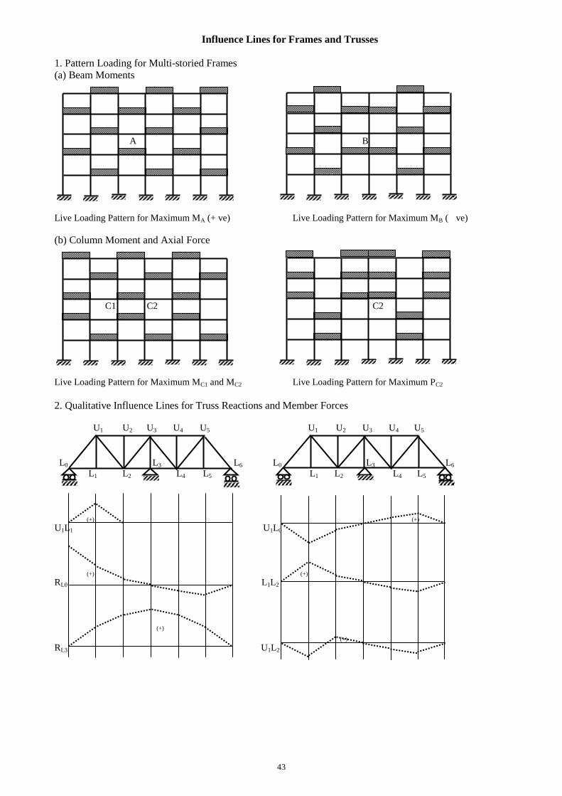
43
Influence Lines for Frames and Trusses
1. Pattern Loading for Multi-storied Frames
(a) Beam Moments
A B
Live Loading Pattern for Maximum MA (+ ve) Live Loading Pattern for Maximum MB ( ve)
(b) Column Moment and Axial Force
C1 C2 C2
Live Loading Pattern for Maximum MC1 and MC2 Live Loading Pattern for Maximum PC2
2. Qualitative Influence Lines for Truss Reactions and Member Forces
U1 U2 U3 U4 U5 U1 U2 U3 U4 U5
L0 L3 L6 L0 L3 L6
L1 L2 L4 L5 L1 L2 L4 L5
(+) (+)
U1L1 U1L0
(+) (+)
RL0 L1L2
(+)
(+)
RL3 U1L2
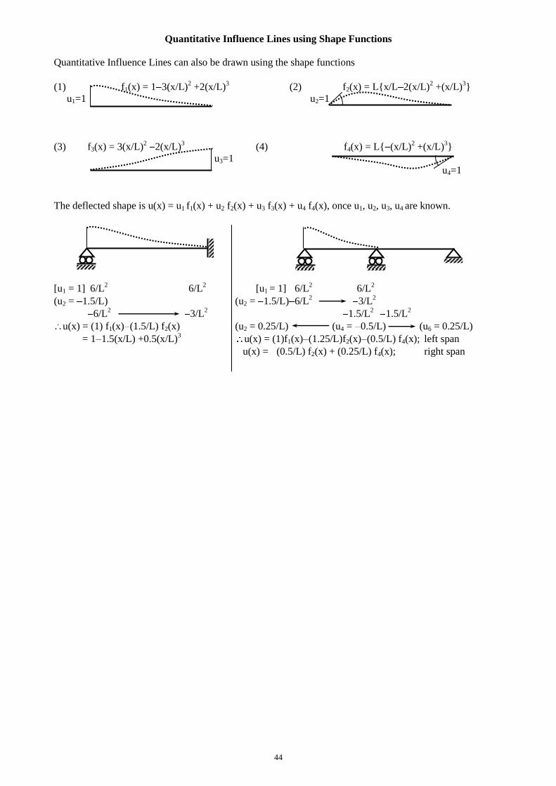
44
Quantitative Influence Lines using Shape Functions
Quantitative Influence Lines can also be drawn using the shape functions
(1) f1(x) = 1 3(x/L)2 +2(x/L)
3 (2) f2(x) = L{x/L 2(x/L)
2 +(x/L)
3}
u1=1 u2=1
(3) f3(x) = 3(x/L)2 2(x/L)
3 (4) f4(x) = L{ (x/L)
2 +(x/L)
3}
u3=1
u4=1
The deflected shape is u(x) = u1 f1(x) + u2 f2(x) + u3 f3(x) + u4 f4(x), once u1, u2, u3, u4 are known.
[u1 = 1] 6/L2
6/L2
[u1 = 1] 6/L2
6/L2
(u2 = 1.5/L) (u2 = 1.5/L) 6/L2
3/L2
6/L2
3/L2
1.5/L
2 1.5/L
2
u(x) = (1) f1(x) (1.5/L) f2(x) (u2 = 0.25/L) (u4 = 0.5/L) (u6 = 0.25/L)
= 1 1.5(x/L) +0.5(x/L)3
u(x) = (1)f1(x) (1.25/L)f2(x) (0.5/L) f4(x); left span
u(x) = (0.5/L) f2(x) + (0.25/L) f4(x); right span
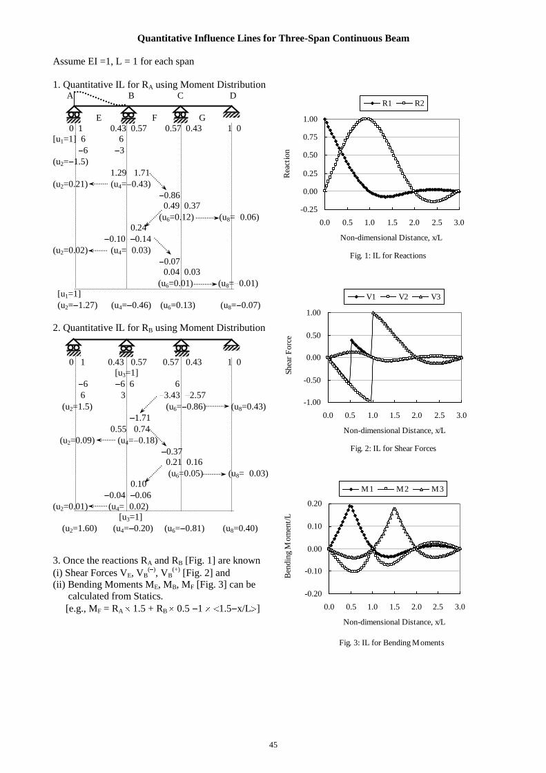
45
Quantitative Influence Lines for Three-Span Continuous Beam
Assume EI =1, L = 1 for each span
1. Quantitative IL for RA using Moment Distribution A B C D
E F G
0 1 0.43 0.57 0.57 0.43 1 0
[u1=1] 6
6
6
3
(u2= 1.5)
1.29 1.71
(u2=0.21) (u4= 0.43)
0.86
0.49 0.37
(u6=0.12) (u8= 0.06)
0.24
0.10 0.14
(u2=0.02) (u4= 0.03)
0.07
0.04 0.03
(u6=0.01) (u8= 0.01)
[u1=1]
(u2= 1.27) (u4= 0.46) (u6=0.13) (u8= 0.07)
2. Quantitative IL for RB using Moment Distribution
0 1 0.43 0.57 0.57 0.43 1 0
[u3=1]
6 6 6 6
6
3 3.43 2.57
(u2=1.5) (u6= 0.86) (u8=0.43)
1.71
0.55 0.74
(u2=0.09) (u4= 0.18)
0.37
0.21 0.16
(u6=0.05) (u8= 0.03)
0.10
0.04 0.06
(u2=0.01) (u4= 0.02)
[u3=1]
(u2=1.60) (u4= 0.20) (u6= 0.81) (u8=0.40)
3. Once the reactions RA and RB [Fig. 1] are known
(i) Shear Forces VE, VB( )
, VB(+)
[Fig. 2] and
(ii) Bending Moments ME, MB, MF [Fig. 3] can be
calculated from Statics.
[e.g., MF = RA 1.5 + RB 0.5 1 1.5 x/L ]
Fig. 1: IL for Reactions
-0.25
0.00
0.25
0.50
0.75
1.00
0.0 0.5 1.0 1.5 2.0 2.5 3.0
Non-dimensional Distance, x/L
Rea
ctio
n
R1 R2
Fig. 2: IL for Shear Forces
-1.00
-0.50
0.00
0.50
1.00
0.0 0.5 1.0 1.5 2.0 2.5 3.0
Non-dimensional Distance, x/L
Shea
r F
orc
eV1 V2 V3
Fig. 3: IL for Bending Moments
-0.20
-0.10
0.00
0.10
0.20
0.0 0.5 1.0 1.5 2.0 2.5 3.0
Non-dimensional Distance, x/L
Ben
din
g M
om
ent/
L
M1 M2 M3
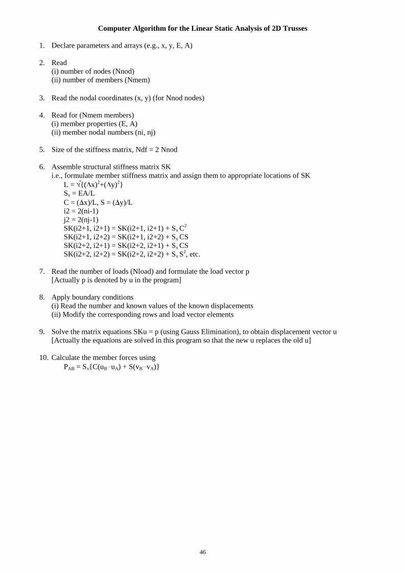
46
Computer Algorithm for the Linear Static Analysis of 2D Trusses
1. Declare parameters and arrays (e.g., x, y, E, A)
2. Read
(i) number of nodes (Nnod)
(ii) number of members (Nmem)
3. Read the nodal coordinates (x, y) (for Nnod nodes)
4. Read for (Nmem members)
(i) member properties (E, A)
(ii) member nodal numbers (ni, nj)
5. Size of the stiffness matrix, Ndf = 2 Nnod
6. Assemble structural stiffness matrix SK
i.e., formulate member stiffness matrix and assign them to appropriate locations of SK
L = {( x)2+( y)
2}
Sx = EA/L
C = ( x)/L, S = ( y)/L
i2 = 2(ni-1)
j2 = 2(nj-1)
SK(i2+1, i2+1) = SK(i2+1, i2+1) + Sx C2
SK(i2+1, i2+2) = SK(i2+1, i2+2) + Sx CS
SK(i2+2, i2+1) = SK(i2+2, i2+1) + Sx CS
SK(i2+2, i2+2) = SK(i2+2, i2+2) + Sx S2, etc.
7. Read the number of loads (Nload) and formulate the load vector p
[Actually p is denoted by u in the program]
8. Apply boundary conditions
(i) Read the number and known values of the known displacements
(ii) Modify the corresponding rows and load vector elements
9. Solve the matrix equations SKu = p (using Gauss Elimination), to obtain displacement vector u
[Actually the equations are solved in this program so that the new u replaces the old u]
10. Calculate the member forces using
PAB = Sx{C(uB uA) + S(vB vA)}
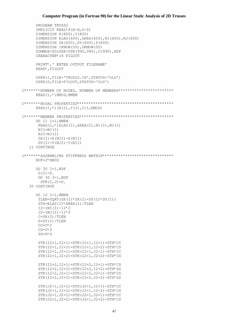
47
Computer Program (in Fortran 90) for the Linear Static Analysis of 2D Trusses
PROGRAM TRUSS2
IMPLICIT REAL*8(A-H,O-Z)
DIMENSION X(800),Y(800)
DIMENSION ELAS(600),AREA(600),NI(600),NJ(600)
DIMENSION DX(600),DY(600),P(600)
DIMENSION IKNOW(50),DKNOW(50)
COMMON/SOLVER/STK(990,990),U(990),NDF
CHARACTER*16 FILOUT
PRINT*,' ENTER OUTPUT FILENAME'
READ*,FILOUT
OPEN(1,FILE='TRUSS2.IN',STATUS='OLD')
OPEN(2,FILE=FILOUT,STATUS='OLD')
C*******NUMBER OF NODES, NUMBER OF MEMBERS************************
READ(1,*)NNOD,NMEM
C*******NODAL PROPERTIES******************************************
READ(1,*)(X(I),Y(I),I=1,NNOD)
C*******MEMBER PROPERTIES*****************************************
DO 11 I=1,NMEM
READ(1,*)ELAS(I),AREA(I),NI(I),NJ(I)
NII=NI(I)
NJI=NJ(I)
DX(I)=X(NJI)-X(NII)
DY(I)=Y(NJI)-Y(NII)
11 CONTINUE
C*******ASSEMBLING STIFFNESS MATRIX*******************************
NDF=2*NNOD
DO 30 I=1,NDF
U(I)=0.
DO 30 J=1,NDF
STK(I,J)=0.
30 CONTINUE
DO 12 I=1,NMEM
TLEN=SQRT(DX(I)*DX(I)+DY(I)*DY(I))
STX=ELAS(I)*AREA(I)/TLEN
I2=(NI(I)-1)*2
J2=(NJ(I)-1)*2
C=DX(I)/TLEN
S=DY(I)/TLEN
CC=C*C
CS=C*S
SS=S*S
STK(I2+1,I2+1)=STK(I2+1,I2+1)+STX*CC
STK(I2+1,I2+2)=STK(I2+1,I2+2)+STX*CS
STK(I2+1,J2+1)=STK(I2+1,J2+1)-STX*CC
STK(I2+1,J2+2)=STK(I2+1,J2+2)-STX*CS
STK(I2+2,I2+1)=STK(I2+2,I2+1)+STX*CS
STK(I2+2,I2+2)=STK(I2+2,I2+2)+STX*SS
STK(I2+2,J2+1)=STK(I2+2,J2+1)-STX*CS
STK(I2+2,J2+2)=STK(I2+2,J2+2)-STX*SS
STK(J2+1,I2+1)=STK(J2+1,I2+1)-STX*CC
STK(J2+1,I2+2)=STK(J2+1,I2+2)-STX*CS
STK(J2+1,J2+1)=STK(J2+1,J2+1)+STX*CC
STK(J2+1,J2+2)=STK(J2+1,J2+2)+STX*CS
48
STK(J2+2,I2+1)=STK(J2+2,I2+1)-STX*CS
STK(J2+2,I2+2)=STK(J2+2,I2+2)-STX*SS
STK(J2+2,J2+1)=STK(J2+2,J2+1)+STX*CS
STK(J2+2,J2+2)=STK(J2+2,J2+2)+STX*SS
12 CONTINUE
C WRITE(2,8)(STK(I,I),I=1,NDF)
C*******LOADS CORRESPONDING TO DEGREES OF FREEDOM**********************
READ(1,*)NLOAD
IF(NLOAD.GT.0)READ(1,*)(J,U(J),I=1,NLOAD)
C*******RESTRAINTS*****************************************************
READ(1,*)NKND
READ(1,*)(IKNOW(I),DKNOW(I),I=1,NKND)
DO 15 I=1,NKND
IKND=IKNOW(I)
DKN=DKNOW(I)
DO 16 J=1,NDF
U(J)=U(J)-STK(J,IKND)*DKN
16 CONTINUE
DO 15 J=1,NDF
IF(J.NE.IKND)THEN
STK(J,IKND)=0.
STK(IKND,J)=0.
ENDIF
U(IKND)=DKN*STK(IKND,IKND)
15 CONTINUE
CALL GAUSS
C*******DISPLACEMENTS**************************************************
6 FORMAT(10(1X,F8.2))
7 FORMAT(1X,I4,10(1X,F10.6))
8 FORMAT(1X,I4,10(1X,F10.4))
WRITE(2,*)'DISPLACEMENTS ARE'
DO 17 I=1,NDF
WRITE(2,7)I,U(I)
17 CONTINUE
C*******MEMBER FORCES**************************************************
WRITE(2,*)
WRITE(2,*)'MEMBER FORCES ARE'
DO 18 I=1,NMEM
TLEN=SQRT(DX(I)*DX(I)+DY(I)*DY(I))
STX=ELAS(I)*AREA(I)/TLEN
I2=(NI(I)-1)*2
J2=(NJ(I)-1)*2
C=DX(I)/TLEN
S=DY(I)/TLEN
AXDIS=(U(J2+1)-U(I2+1))*C+(U(J2+2)-U(I2+2))*S
P(I)=STX*AXDIS
WRITE(2,8)I,P(I)
18 CONTINUE
END
49
C**********************************************************************
C*******GAUSS ELIMINATION**********************************************
SUBROUTINE GAUSS
IMPLICIT REAL*8(A-H,O-Z)
COMMON/SOLVER/A(990,990),B(990),N
NHBW=N
N1=N-1
DO 10 K=1,N1
K1=K+1
KH=K+NHBW
C=1./A(K,K)
DO 11 I=K1,KH
IF(I.LE.N)D=A(I,K)*C
DO 12 J=K1,KH
12 IF(J.LE.N)A(I,J)=A(I,J)-D*A(K,J)
11 IF(I.LE.N)B(I)=B(I)-D*B(K)
10 CONTINUE
B(N)=B(N)/A(N,N)
DO 13 I=N1,1,-1
I1=I+1
SUM=0.
DO 14 K=I1,N
14 SUM=SUM+A(I,K)*B(K)
13 B(I)=(B(I)-SUM)/A(I,I)
END
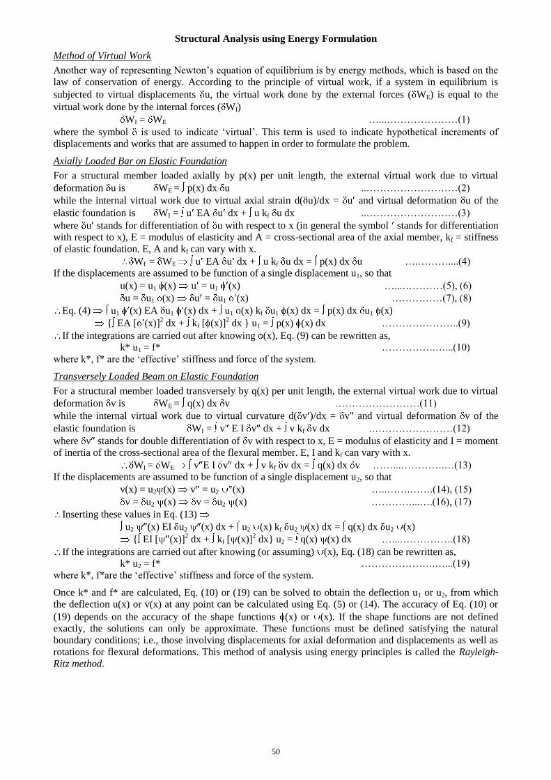
50
Structural Analysis using Energy Formulation
Method of Virtual Work
Another way of representing Newton’s equation of equilibrium is by energy methods, which is based on the
law of conservation of energy. According to the principle of virtual work, if a system in equilibrium is
subjected to virtual displacements u, the virtual work done by the external forces ( WE) is equal to the
virtual work done by the internal forces ( WI)
WI = WE …...…………………(1)
where the symbol is used to indicate ‘virtual’. This term is used to indicate hypothetical increments of
displacements and works that are assumed to happen in order to formulate the problem.
Axially Loaded Bar on Elastic Foundation
For a structural member loaded axially by p(x) per unit length, the external virtual work due to virtual
deformation u is WE = p(x) dx u ..………………………(2)
while the internal virtual work due to virtual axial strain d( u)/dx = u and virtual deformation u of the
elastic foundation is WI = u EA u dx + u kf u dx ..………………………(3)
where u stands for differentiation of u with respect to x (in general the symbol stands for differentiation
with respect to x), E = modulus of elasticity and A = cross-sectional area of the axial member, kf = stiffness
of elastic foundation. E, A and kf can vary with x.
WI = WE u EA u dx + u kf u dx = p(x) dx u ….………....(4)
If the displacements are assumed to be function of a single displacement u1, so that
u(x) = u1 (x) u = u1 (x) …...…………(5), (6)
u = u1 (x) u = u1 (x) ……………(7), (8)
Eq. (4) u1 (x) EA u1 (x) dx + u1 (x) kf u1 (x) dx = p(x) dx u1 (x)
{ EA [ (x)]2 dx + kf [ (x)]
2 dx } u1 = p(x) (x) dx …………………..(9)
If the integrations are carried out after knowing (x), Eq. (9) can be rewritten as,
k* u1 = f* …………….…...(10)
where k*, f* are the ‘effective’ stiffness and force of the system.
Transversely Loaded Beam on Elastic Foundation
For a structural member loaded transversely by q(x) per unit length, the external virtual work due to virtual
deformation v is WE = q(x) dx v .……………………(11)
while the internal virtual work due to virtual curvature d( v )/dx = v and virtual deformation v of the
elastic foundation is WI = v E I v dx + v kf v dx .……………………(12)
where v stands for double differentiation of v with respect to x, E = modulus of elasticity and I = moment
of inertia of the cross-sectional area of the flexural member. E, I and kf can vary with x.
WI = WE v E I v dx + v kf v dx = q(x) dx v ……...………….…(13)
If the displacements are assumed to be function of a single displacement u2, so that
v(x) = u2 (x) v = u2 (x) …..…….…….(14), (15)
v = u2 (x) v = u2 (x) …………...….(16), (17)
Inserting these values in Eq. (13)
u2 (x) EI u2 (x) dx + u2 (x) kf u2 (x) dx = q(x) dx u2 (x)
{ EI [ (x)]2 dx + kf [ (x)]
2 dx} u2 = q(x) (x) dx …...…………….(18)
If the integrations are carried out after knowing (or assuming) (x), Eq. (18) can be rewritten as,
k* u2 = f* ………………….…...(19)
where k*, f*are the ‘effective’ stiffness and force of the system.
Once k* and f* are calculated, Eq. (10) or (19) can be solved to obtain the deflection u1 or u2, from which
the deflection u(x) or v(x) at any point can be calculated using Eq. (5) or (14). The accuracy of Eq. (10) or
(19) depends on the accuracy of the shape functions (x) or (x). If the shape functions are not defined
exactly, the solutions can only be approximate. These functions must be defined satisfying the natural
boundary conditions; i.e., those involving displacements for axial deformation and displacements as well as
rotations for flexural deformations. This method of analysis using energy principles is called the Rayleigh-
Ritz method.
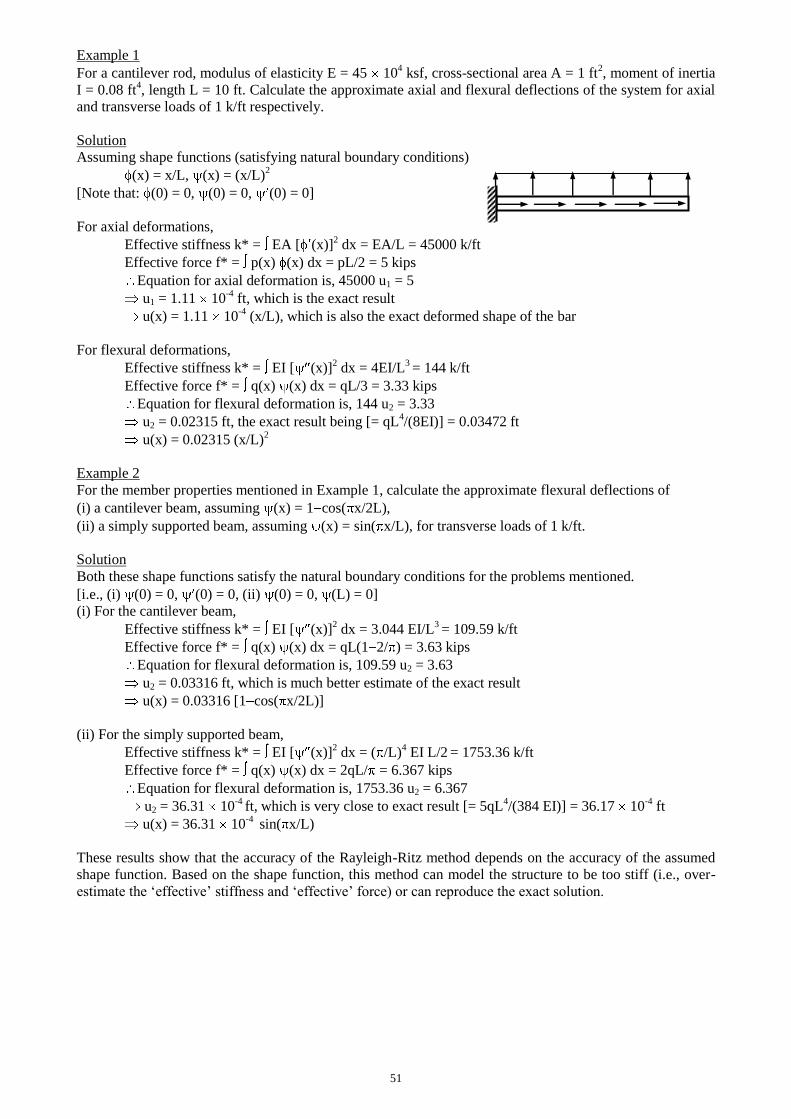
51
Example 1
For a cantilever rod, modulus of elasticity E = 45 104 ksf, cross-sectional area A = 1 ft
2, moment of inertia
I = 0.08 ft4, length L = 10 ft. Calculate the approximate axial and flexural deflections of the system for axial
and transverse loads of 1 k/ft respectively.
Solution
Assuming shape functions (satisfying natural boundary conditions)
(x) = x/L, (x) = (x/L)2
[Note that: (0) = 0, (0) = 0, (0) = 0]
For axial deformations,
Effective stiffness k* = EA [ (x)]2 dx = EA/L = 45000 k/ft
Effective force f* = p(x) (x) dx = pL/2 = 5 kips
Equation for axial deformation is, 45000 u1 = 5
u1 = 1.11 10-4
ft, which is the exact result
u(x) = 1.11 10
-4 (x/L), which is also the exact deformed shape of the bar
For flexural deformations,
Effective stiffness k* = EI [ (x)]2 dx = 4EI/L
3 = 144 k/ft
Effective force f* = q(x) (x) dx = qL/3 = 3.33 kips
Equation for flexural deformation is, 144 u2 = 3.33
u2 = 0.02315 ft, the exact result being [= qL4/(8EI)] = 0.03472 ft
u(x) = 0.02315 (x/L)2
Example 2
For the member properties mentioned in Example 1, calculate the approximate flexural deflections of
(i) a cantilever beam, assuming (x) = 1 cos( x/2L),
(ii) a simply supported beam, assuming (x) = sin( x/L), for transverse loads of 1 k/ft.
Solution
Both these shape functions satisfy the natural boundary conditions for the problems mentioned.
[i.e., (i) (0) = 0, (0) = 0, (ii) (0) = 0, (L) = 0]
(i) For the cantilever beam,
Effective stiffness k* = EI [ (x)]2 dx = 3.044 EI/L
3 = 109.59 k/ft
Effective force f* = q(x) (x) dx = qL(1 2/ ) = 3.63 kips
Equation for flexural deformation is, 109.59 u2 = 3.63
u2 = 0.03316 ft, which is much better estimate of the exact result
u(x) = 0.03316 [1 cos( x/2L)]
(ii) For the simply supported beam,
Effective stiffness k* = EI [ (x)]2 dx = ( /L)
4 EI L/2
= 1753.36 k/ft
Effective force f* = q(x) (x) dx = 2qL/ = 6.367 kips
Equation for flexural deformation is, 1753.36 u2 = 6.367
u2 = 36.31 10-4
ft, which is very close to exact result [= 5qL4/(384 EI)] = 36.17 10
-4 ft
u(x) = 36.31 10-4
sin( x/L)
These results show that the accuracy of the Rayleigh-Ritz method depends on the accuracy of the assumed
shape function. Based on the shape function, this method can model the structure to be too stiff (i.e., over-
estimate the ‘effective’ stiffness and ‘effective’ force) or can reproduce the exact solution.
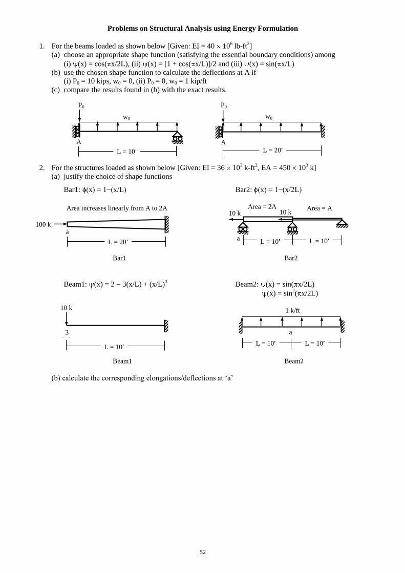
52
Problems on Structural Analysis using Energy Formulation
1. For the beams loaded as shown below [Given: EI = 40 106 lb-ft
2]
(a) choose an appropriate shape function (satisfying the essential boundary conditions) among
(i) (x) = cos( x/2L), (ii) (x) = [1 + cos( x/L)]/2 and (iii) (x) = sin( x/L)
(b) use the chosen shape function to calculate the deflections at A if
(i) P0 = 10 kips, w0 = 0, (ii) P0 = 0, w0 = 1 kip/ft
(c) compare the results found in (b) with the exact results.
2. For the structures loaded as shown below [Given: EI = 36 103 k-ft
2, EA = 450 10
3 k]
(a) justify the choice of shape functions
Bar1: (x) = 1−(x/L) Bar2: (x) = 1−(x/2L)
Bar1 Bar2
Beam1: (x) = 2 3(x/L) + (x/L)3 Beam2: (x) = sin( x/2L)
(x) = sin2( x/2L)
Beam1 Beam2
(b) calculate the corresponding elongations/deflections at ‘a’
a
w0 w0
A A
L = 20 L = 10 L = 10
L = 10 L = 10
L = 20 L = 10
P0 P0
10 k 10 k Area = 2A Area = A
100 k
Area increases linearly from A to 2A
a
3
k/ft
a
a
10 k 1 k/ft
L = 10

53
Problems on Structural Analysis using Energy Formulation
1. (a) For (x) = cos( x/2L), (0) = cos(0) = 1 (0) = ( /2L) sin(0) = 0
(L) = cos( /2) = 0 (L) = ( /2L) sin( /2) = ( /2L)
For (x) = [1 + cos( x/L)]/2, (0) = [1 + 1]/2 = 1 (0) = ( /L) sin(0) = 0
(L) = [1 1]/2 = 0 (L) = ( /L) sin( ) = 0
For (x) = sin( x/L), (0) = sin(0) = 0 (0) = ( /L) cos(0) = /L
(L) = sin( ) = 0 (L) = ( /L) cos( ) = /L
For the first beam
(0) 0, (0) = 0, (L) = 0, (L) 0; Choose (x) = cos( x/2L)
For the second beam
(0) 0, (0) = 0, (L) = 0, (L) = 0; Choose (x) = [1 + cos( x/L)]/2
Since (0) = 1 for both these functions, the deflection u2 indicates uA here
(b) For the first beam, (x) = cos( x/2L) (x) = ( /2L)2 cos( x/2L)
Effective stiffness k* = EI [ (x)]2 dx = ( /2L)
4 EI L/2
= 121.76 k/ft
For P0 = 10 kips, Effective force f* = q(x) (x) dx = ( 10) (0) = 10 kips
u2 = 10/121.76 = 0.0821 ft = 0.986 in
For w0 = 1 kip/ft, Effective force f* = q(x) (x) dx = (1) (2 10/ ) (1) = 6.366 kips
u2 = 6.366/121.76 = 0.0523 ft = 0.627 in
For the second beam, (x) = [1 + cos( x/L)]/2 (x) = ( /L)2 cos( x/L)/2
Effective stiffness k* = EI [ (x)]2 dx = [( /L)
4/4] EI L/2
= 60.88 k/ft
For P0 = 10 kips, Effective force f* = q(x) (x) dx = ( 10) (0) = 10 kips
u2 = 10/60.88 = 0.164 ft = 1.971 in
For w0 = 1 kip/ft, Effective force f* = q(x) (x) dx = (1) (20)/2 = 10 kips
u2 = 10/60.88 = 0.164 ft = 1.971 in
(c) The exact results are (using Stiffness Method)
For the first beam, u2 = 1.0 in and 0.625 in
For the second beam, u2 = 2.0 in and 2.0 in
w0 w0
A A
L = 20 L = 10
P0 P0

54
2. (a) For Bar1, (0) 0, (L) = 0
(x) = 1−(x/L) (0) = 1 0, (L) = 0 OK
For Bar2, (0) 0, (L) 0, (2L) = 0
(x) = 1−(x/2L) (0) = 1 0, (L) = 0.5 0, (2L) = 0 OK
For Beam1, (0) 0, (0) 0, (L) = 0, (L) = 0
(x) = 2 3(x/L) + (x/L)3, (x) = 3/L + 3x
2/L
3
(0) = 2, (0) = 3/L 0, (L) = 2 3 + 1 = 0, (L) = 3/L + 3L2/L
3 = 0 OK
For Beam2, (0) = 0, (0) = 0, (2L) = 0, (2L) = 0
(x) = sin( x/2L), (x) = ( /2L) cos( x/2L)
(0) = 0, (0) = /2L, (2L) = sin( ) = 0, (2L) = ( /2L) cos( ) = ( /2L) Not OK
(x) = sin2( x/2L) = [1 cos( x/L)]/2, (x) = ( /2L) sin( x/L)
(0) = 0, (0) = /2L sin (0) = 0, (2L) = sin2( ) = 0, (2L) = ( /2L) sin(2 )
= 0 OK
Bar1 Bar2
Beam1 Beam2
(b) For Bar1, A(x) = A (1 + x/L), (x) = 1/L
Effective stiffness k* = EA[ (x)]2 dx = EA (L + L
2/2L)/L
2 = 33.75 10
3 k/ft
Effective force f* = p(x) (x) dx = (100) (0) = 100 kips
u1 = 100/(33.75 103) = 2.96 10
3 ft = 0.0356 in ua = u1 (0) = 0.0356 in
For Bar2, A1 = 2A, A2 = A, (x) = 1/2L
Effective stiffness k* = EA [ (x)]2 dx = (E/4L
2) (2A L + A L) = 3 EA/4L = 33.75 10
3 k/ft
Effective force f*= p(x) (x)dx = ( 10) (0)+ ( 10) (L) = ( 10) (1) + ( 10) (0.5) = 15 kips
u1 = 15/(33.75 103) = 4.44 10
4 ft = 5.33 10
3 in ua = u1 (0) = 5.33 10
3 in
For Beam1, (x) = 2 3(x/L) + (x/L)3, (x) = 3/L + 3 x
2/L
3, (x) = 6 x/L
3
Effective stiffness k* = EI [ (x)]2 dx = EI 36 x
2/L
6 dx = 12 EI/L
3 = 432 k/ft
Effective force f* = q(x) (x) dx = ( 10) (0) = ( 10) (2) = 20 kips
u2 = 20/432 = 0.0463 ft = 0.556
in ua = u2 (0) = 0.556 2 = 1.111 in
For Beam2, (x) = [1 cos( x/L)]/2, (x) = ( /2L) sin( x/L), (x) = [( /L)2 cos( x/L)]/2
Effective stiffness k*= EI [ (x)]2 dx = EI ( /L)
4[cos
2( x/L)]/4 dx =
4EI/(4L
3)= 876.68 k/ft
Effective force f* = q(x) (x) dx = (1) [1 cos( x/L)]/2 dx = 10 kips
u2 = 10/876.68 = 0.0114 ft = 0.137
in ua = u2 (L) = 0.137 1 = 0.137 in
a
L = 20 L = 10 L = 10
L = 10 L = 10
10 k 10 k Area = 2A Area = A
100 k
Area increases linearly from A to 2A
a
a a
10 k 1 k/ft
L = 10
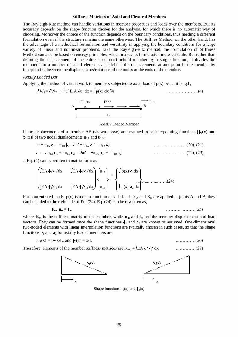
55
Stiffness Matrices of Axial and Flexural Members
The Rayleigh-Ritz method can handle variations in member properties and loads over the members. But its
accuracy depends on the shape function chosen for the analysis, for which there is no automatic way of
choosing. Moreover the choice of the function depends on the boundary conditions, thus needing a different
formulation even if the structure remains the same otherwise. The Stiffnes Method, on the other hand, has
the advantage of a methodical formulation and versatility in applying the boundary conditions for a large
variety of linear and nonlinear problems. Like the Rayleigh-Ritz method, the formulation of Stiffness
Method can also be based on energy principles, which makes its formulation more versatile. But rather than
defining the displacement of the entire structure/structural member by a single function, it divides the
member into a number of small elements and defines the displacements at any point in the member by
interpolating between the displacements/rotations of the nodes at the ends of the member.
Axially Loaded Bar
Applying the method of virtual work to members subjected to axial load of p(x) per unit length,
WI = WE u E A u dx = p(x) dx u …………………(4)
u1A p(x) u1B
A B
L
Axially Loaded Member
If the displacements of a member AB (shown above) are assumed to be interpolating functions [ 1(x) and
2(x)] of two nodal displacements u1A and u1B,
u = u1A 1 + u1B 2 u = u1A 1 + u1B 2 …………..………(20), (21)
u = u1A 1 + u1B 2 u = u1A 1 + u1B 2 …...……..……….(22), (23)
Eq. (4) can be written in matrix form as,
EA 1 1 dx EA 1 2 dx u1A p(x) 1dx
……....…...…….(24)
EA 2 1 dx EA 2 2 dx u1B p(x) 2 dx
For concentrated loads, p(x) is a delta function of x. If loads XA and XB are applied at joints A and B, they
can be added to the right side of Eq. (24). Eq. (24) can be rewritten as,
Km um = fm ………...………(25)
where Km is the stiffness matrix of the member, while um and fm are the member displacement and load
vectors. They can be formed once the shape functions 1 and 2 are known or assumed. One-dimensional
two-noded elements with linear interpolation functions are typically chosen in such cases, so that the shape
functions 1 and 2 for axially loaded members are
1(x) = 1 x/L, and 2(x) = x/L ..…………(26)
Therefore, elements of the member stiffness matrices are Kmij = EA i
j dx ..…………(27)
1(x) 2(x)
x x
Shape functions 1(x) and 2(x)
=
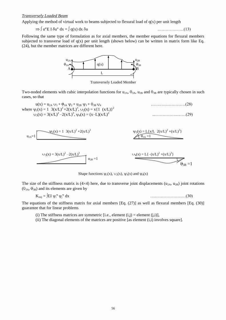
56
Transversely Loaded Beam
Applying the method of virtual work to beams subjected to flexural load of q(x) per unit length
u E I u dx = q(x) dx u .………………(13)
Following the same type of formulation as for axial members, the member equations for flexural members
subjected to transverse load of q(x) per unit length (shown below) can be written in matrix form like Eq.
(24), but the member matrices are different here.
u2A u2B
3A q(x) 3B
A B
L
Transversely Loaded Member
Two-noded elements with cubic interpolation functions for u2A, 3A, u2B and 3B are typically chosen in such
cases, so that
u(x) = u2A 1 + 3A 2 + u2B 3 + 3B 4 …….………………(28)
where 1(x) = 1 3(x/L)2 +2(x/L)
3, 2(x) = x{1 (x/L)}
2
3(x) = 3(x/L)2
2(x/L)3, 4(x) = (x L)(x/L)
2 ...…………….……(29)
1(x) = 1 3(x/L)2 +2(x/L)
3 2(x) = L{x/L 2(x/L)
2 +(x/L)
3}
u2A=1 3A =1
3(x) = 3(x/L)2 2(x/L)
3 4(x) = L{ (x/L)
2 +(x/L)
3}
u2B =1
3B =1
Shape functions 1(x), 2(x), 3(x) and 4(x)
The size of the stiffness matrix is (4 4) here, due to transverse joint displacements (u2A, u2B) joint rotations
( 3A, 3B) and its elements are given by
Kmij = EI i
j dx …..…………………(30)
The equations of the stiffness matrix for axial members [Eq. (27)] as well as flexural members [Eq. (30)]
guarantee that for linear problems
(i) The stiffness matrices are symmetric [i.e., element (i,j) = element (j,i)],
(ii) The diagonal elements of the matrices are positive [as element (i,i) involves square].
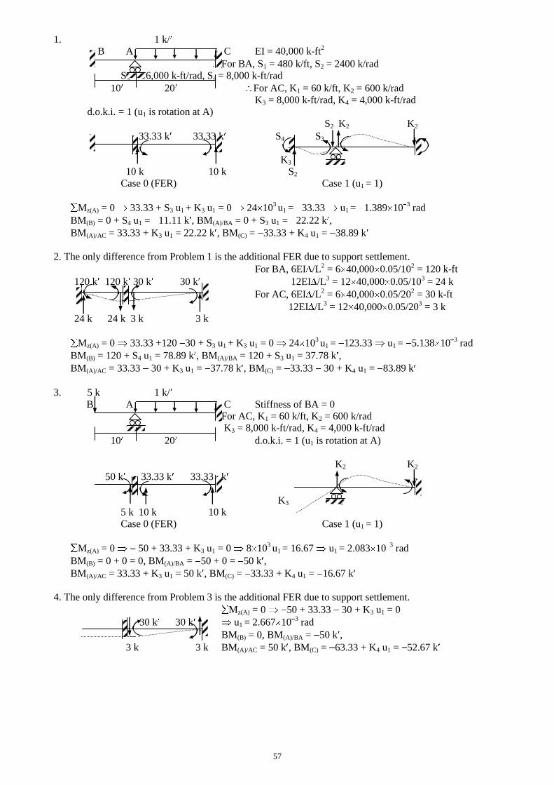
57
1. 1 k/
B A C EI = 40,000 k-ft2
For BA, S1 = 480 k/ft, S2 = 2400 k/rad
S3 = 16,000 k-ft/rad, S4 = 8,000 k-ft/rad
10 20 For AC, K1 = 60 k/ft, K2 = 600 k/rad
K3 = 8,000 k-ft/rad, K4 = 4,000 k-ft/rad
d.o.k.i. = 1 (u1 is rotation at A)
S2 K2 K2
33.33 k 33.33 k S4 S3
K3 K4
10 k 10 k S2
Case 0 (FER) Case 1 (u1 = 1)
Mz(A) = 0 33.33 + S3 u1 + K3 u1 = 0 24 103 u1 = 33.33 u1 = 1.389 10
3 rad
BM(B) = 0 + S4 u1 = 11.11 k , BM(A)/BA = 0 + S3 u1 = 22.22 k ,
BM(A)/AC = 33.33 + K3 u1 = 22.22 k , BM(C) = 33.33 + K4 u1 = 38.89 k
2. The only difference from Problem 1 is the additional FER due to support settlement.
For BA, 6EI /L2 = 6 40,000 0.05/10
2 = 120 k-ft
120 k 120 k 30 k 30 k 12EI /L3 = 12 40,000 0.05/10
3 = 24 k
For AC, 6EI /L2 = 6 40,000 0.05/20
2 = 30 k-ft
12EI /L3 = 12 40,000 0.05/20
3 = 3 k
24 k 24 k 3 k 3 k
Mz(A) = 0 33.33 +120 30 + S3 u1 + K3 u1 = 0 24 103 u1 = 123.33 u1 = 5.138 10
3 rad
BM(B) = 120 + S4 u1 = 78.89 k , BM(A)/BA = 120 + S3 u1 = 37.78 k ,
BM(A)/AC = 33.33 30 + K3 u1 = 37.78 k , BM(C) = 33.33 30 + K4 u1 = 83.89 k
3. 5 k 1 k/
B A C Stiffness of BA = 0
For AC, K1 = 60 k/ft, K2 = 600 k/rad
K3 = 8,000 k-ft/rad, K4 = 4,000 k-ft/rad
10 20 d.o.k.i. = 1 (u1 is rotation at A)
K2 K2
50 k 33.33 k 33.33 k
K3 K4
5 k 10 k 10 k Case 0 (FER) Case 1 (u1 = 1)
Mz(A) = 0 50 + 33.33 + K3 u1 = 0 8 103 u1 = 16.67 u1 = 2.083 10
3 rad
BM(B) = 0 + 0 = 0, BM(A)/BA = 50 + 0 = 50 k ,
BM(A)/AC = 33.33 + K3 u1 = 50 k , BM(C) = 33.33 + K4 u1 = 16.67 k
4. The only difference from Problem 3 is the additional FER due to support settlement.
Mz(A) = 0 50 + 33.33 30 + K3 u1 = 0
30 k 30 k u1 = 2.667 103 rad
BM(B) = 0, BM(A)/BA = 50 k ,
3 k 3 k BM(A)/AC = 50 k , BM(C) = 63.33 + K4 u1 = 52.67 k
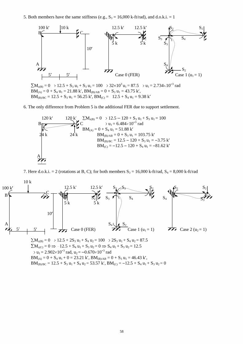
58
5. Both members have the same stiffness (e.g., S3 = 16,000 k-ft/rad), and d.o.k.i. = 1
100 k 10 k 12.5 k 12.5 k S2 S2
B C
S2 S3 S4
5 k 5 k S3
10
A S4
S2
5 5 Case 0 (FER) Case 1 (u1 = 1)
Mz(B) = 0 12.5 + S3 u1 + S3 u1 = 100 32 103 u1 = 87.5 u1 = 2.734 10
3 rad
BM(A) = 0 + S4 u1 = 21.88 k , BM(B)/AB = 0 + S3 u1 = 43.75 k ,
BM(B)/BC = 12.5 + S3 u1 = 56.25 k , BM(C) = 12.5 + S4 u1 = 9.38 k
6. The only difference from Problem 5 is the additional FER due to support settlement.
120 k 120 k Mz(B) = 0 12.5 120 + S3 u1 + S3 u1 = 100
B C u1 = 6.484 103 rad
BM(A) = 0 + S4 u1 = 51.88 k
24 k 24 k BM(B)/AB = 0 + S3 u1 = 103.75 k
BM(B)/BC = 12.5 120 + S3 u1 = 3.75 k
BM(C) = 12.5 120 + S4 u1 = 81.62 k
A
7. Here d.o.k.i. = 2 (rotations at B, C); for both members S3 = 16,000 k-ft/rad, S4 = 8,000 k-ft/rad
10 k
12.5 k 12.5 k S2 S3 S2 S2 S2
C
S2 S3 S4 S4
5 k 5 k
10
S4 S2
5 Case 0 (FER) Case 1 (u1 = 1) Case 2 (u2 = 1)
Mz(B) = 0 12.5 + 2S3 u1 + S4 u2 = 100 2S3 u1 + S4 u2 = 87.5
Mz(C) = 0 12.5 + S4 u1 + S3 u2 = 0 S4 u1 + S3 u2 = 12.5
u1 = 2.902 103 rad, u2 = 0.670 10
3 rad
BM(A) = 0 + S4 u1 + 0 = 23.21 k , BM(B)/AB = 0 + S3 u1 = 46.43 k ,
BM(B)/BC = 12.5 + S3 u1 + S4 u2 = 53.57 k , BM(C) = 12.5 + S4 u1 + S3 u2 = 0
100 k
B
A
5
S3
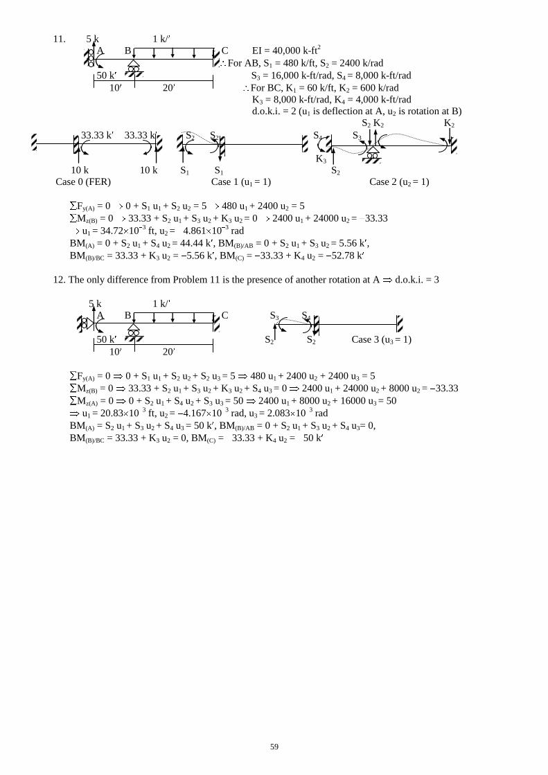
59
11. 5 k 1 k/
A B C EI = 40,000 k-ft2
For AB, S1 = 480 k/ft, S2 = 2400 k/rad
50 k S3 = 16,000 k-ft/rad, S4 = 8,000 k-ft/rad
10 20 For BC, K1 = 60 k/ft, K2 = 600 k/rad
K3 = 8,000 k-ft/rad, K4 = 4,000 k-ft/rad
d.o.k.i. = 2 (u1 is deflection at A, u2 is rotation at B)
S2 K2 K2
33.33 k 33.33 k S2 S2 S4 S3
K3 K4
10 k 10 k S1 S1 S2
Case 0 (FER) Case 1 (u1 = 1) Case 2 (u2 = 1)
Fy(A) = 0 0 + S1 u1 + S2 u2 = 5 480 u1 + 2400 u2 = 5
Mz(B) = 0 33.33 + S2 u1 + S3 u2 + K3 u2 = 0 2400 u1 + 24000 u2 = 33.33
u1 = 34.72 103 ft, u2 = 4.861 10
3 rad
BM(A) = 0 + S2 u1 + S4 u2 = 44.44 k , BM(B)/AB = 0 + S2 u1 + S3 u2 = 5.56 k ,
BM(B)/BC = 33.33 + K3 u2 = 5.56 k , BM(C) = 33.33 + K4 u2 = 52.78 k
12. The only difference from Problem 11 is the presence of another rotation at A d.o.k.i. = 3
5 k 1 k/
A B C S3 S4
50 k S2 S2 Case 3 (u3 = 1)
10 20
Fy(A) = 0 0 + S1 u1 + S2 u2 + S2 u3 = 5 480 u1 + 2400 u2 + 2400 u3 = 5
Mz(B) = 0 33.33 + S2 u1 + S3 u2 + K3 u2 + S4 u3 = 0 2400 u1 + 24000 u2 + 8000 u2 = 33.33
Mz(A) = 0 0 + S2 u1 + S4 u2 + S3 u3 = 50 2400 u1 + 8000 u2 + 16000 u3 = 50
u1 = 20.83 103 ft, u2 = 4.167 10
3 rad, u3 = 2.083 10
3 rad
BM(A) = S2 u1 + S3 u2 + S4 u3 = 50 k , BM(B)/AB = 0 + S2 u1 + S3 u2 + S4 u3= 0,
BM(B)/BC = 33.33 + K3 u2 = 0, BM(C) = 33.33 + K4 u2 = 50 k
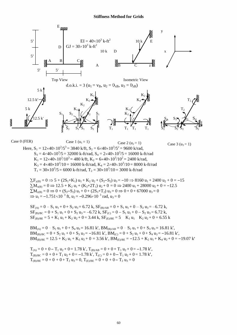
60
Stiffness Method for Grids
E y
5 EI = 40 103 k-ft
2 10 k E
GJ = 30 103 k-ft
2
10 k D x
5 A B C A B C z 5 5
Top View Isometric View
d.o.k.i. = 3 (u1 = vB, u2 = xB, u3 = zB) 5 k
K1 K2 12.5 k K2 K4 T2 K2 5 k K1 K3 T2 S1 S2 S2 S1 K2 12.5 k S4 S3 S3 S4
S2 S1 S1 S2 T1 T1 T1 T1 S2 S2 S2 S2
Here, S1 = 12 40 103/5
3 = 3840 k/ft, S2 = 6 40 10
3/5
2 = 9600 k/rad,
S3 = 4 40 103/5
= 32000 k-ft/rad, S4 = 2 40 10
3/5
= 16000 k-ft/rad
K1 = 12 40 103/10
3 = 480 k/ft, K2 = 6 40 10
3/10
2 = 2400 k/rad,
K3 = 4 40 103/10
= 16000 k-ft/rad, K4 = 2 40 10
3/10
= 8000 k-ft/rad
T1 = 30 103/5
= 6000 k-ft/rad, T2 = 30 10
3/10
= 3000 k-ft/rad
Fy(B) = 0 5 + (2S1+K1) u1 + K2 u2 + (S2 S2) u3 = 10 8160 u1 + 2400 u2 + 0 = 15
Mx(B) = 0 12.5 + K2 u1 + (K3+2T1) u2 + 0 = 0 2400 u1 + 28000 u2 + 0 = 12.5
Mz(B) = 0 0 + (S2 S2) u1 + 0 + (2S3+T2) u3 = 0 0 + 0 + 67000 u3 = 0
u1 = 1.751 103 ft, u2 = 0.296 10
3 rad, u3 = 0
SF(A) = 0 S1 u1 + 0 + S2 u3 = 6.72 k, SF(B)/AB = 0 + S1 u1 + 0 S2 u3 = 6.72 k,
SF(B)/BC = 0 + S1 u1 + 0 + S2 u3 = 6.72 k, SF(C) = 0 S1 u1 + 0 S2 u3 = 6.72 k,
SF(B)/BE = 5 + K1 u1 + K2 u2 + 0 = 3.44 k, SF(E)/BE = 5 K1 u1 K2 u2 + 0 = 6.55 k
BM(A) = 0 S2 u1 + 0 + S4 u3 = 16.81 k , BM(B)/AB = 0 S2 u1 + 0 + S3 u3 = 16.81 k ,
BM(B)/BC = 0 + S2 u1 + 0 + S3 u3 = 16.81 k , BM(C) = 0 + S2 u1 + 0 + S4 u3 = 16.81 k ,
BM(B)/BE = 12.5 + K2 u1 + K3 u2 + 0 = 3.56 k , BM(E)/BE = 12.5 + K2 u1 + K4 u2 + 0 = 19.07 k
T(A) = 0 + 0 T1 u2 + 0 = 1.78 k , T(B)/AB = 0 + 0 + T1 u2 + 0 = 1.78 k ,
T(B)/BC = 0 + 0 + T1 u2 + 0 = 1.78 k , T(C) = 0 + 0 T1 u2 + 0 = 1.78 k ,
T(B)/BE = 0 + 0 + 0 + T2 u3 = 0, T(E)/BE = 0 + 0 + 0 T2 u3 = 0
D
Case 0 (FER) Case 1 (u1 = 1) Case 2 (u2 = 1) Case 3 (u3 = 1)

61
Problems on Stiffness Method for Grids
Given: EI = 40 103 k-ft
2, GJ = 30 10
3 k-ft
2 for all the problems.
1,2. Use the Stiffness Method to calculate the rotations at joint C for the grids shown below.
Problem 1 Problem 2
3. Using the Stiffness Method, calculate the deflection and rotation at joint C for the grid shown in the
figure below.
A
15
10 10
B C D
5
10 k
4, 5. Formulate the stiffness matrix and load vector for the grids shown in the figures below.
A
B C D
10 10 5 5
Problem 4 Problem 5
E
1 k/ft
10 k
10 15
C
15
5
E
A
10 10
D B
10 k
10 15
5
E
D
C
B
A
1 k/ft
10