Structural Analysis Bab 12

7/18/2019 Structural Analysis Bab 12

http://slidepdf.com/reader/full/structural-analysis-bab-12 1/37

12

Approximate Analysis ofRectangular Building Frames12.1 Assumptions for Approximate Analysis

12.2 Analysis for Vertical Loads

12.3 Analysis for Lateral Loads—Portal Method

12.4 Analysis for Lateral Loads—Cantilever Method

SummaryProblems

St. Louis Gateway Arch and Old CourthouseR. Gino Santa Maria/Shutterstock

471

The analysis of statically indeterminate structures using the force anddisplacement methods introduced in the preceding chapter can be con-sidered as exact in the sense that the compatibility and equilibrium

conditions of the structure are exactly satisfied in such an analysis.However, the results of such an exact analysis represent the actualstructural response only to the extent that the analytical model of thestructure represents the actual structure. Experimental results havedemonstrated that the response of most common types of structuresunder service loads can be reliably predicted by the force and displace-ment methods, provided an accurate analytical model of the structure isused in the analysis.

Exact analysis of indeterminate structures involves computationof deflections and solution of simultaneous equations, so it can be quitetime consuming. Moreover, such an analysis depends on the relativesizes (cross-sectional areas and/or moments of inertia) of the membersof the structure. Because of these di‰culties associated with the exactanalysis, the preliminary designs of indeterminate structures are oftenbased on the results of approximate analysis, in which the internal forcesare estimated by making certain assumptions about the deformationsand/or the distribution of forces between the members of structures,

thereby avoiding the necessity of computing deflections.



Approximate analysis proves to be quite convenient to use in theplanning phase of projects, when several alternative designs of thestructure are usually evaluated for relative economy. The results of ap-proximate analysis can also be used to estimate the sizes of variousstructural members needed to initiate the exact analysis. The prelimi-nary designs of members are then revised iteratively, using the results of successive exact analyses, to arrive at their final designs. Furthermore,approximate analysis is sometimes used to roughly check the resultsof exact analysis, which due to its complexity can be prone to errors.Finally, in recent years, there has been an increased tendency towardrenovating and retrofitting older structures. Many such structures con-structed prior to 1960, including many high-rise buildings, were de-

signed solely on the basis of approximate analysis, so a knowledge andunderstanding of approximate methods used by the original designers isusually helpful in a renovation undertaking.

Unlike the exact methods, which are general in the sense that theycan be applied to various types of structures subjected to various load-ing conditions, a specific method is usually required for the approximateanalysis of a particular type of structure for a particular loading. Forexample, a di¤erent approximate method must be employed for theanalysis of a rectangular frame under vertical (gravity) loads than forthe analysis of the same frame subjected to lateral loads. Numerousmethods have been developed for approximate analysis of indeterminatestructures. Some of the more common approximate methods pertainingto rectangular frames are presented in this chapter. These methods canbe expected to yield results within 20% of the exact solutions.

The objectives of this chapter are to consider the approximateanalysis of rectangular building frames as well as to gain an under-standing of the techniques used in the approximate analysis of struc-

tures in general. We present a general discussion of the simplifyingassumptions necessary for approximate analysis and then consider theapproximate analysis of rectangular frames under vertical (gravity)loads. Finally, we present the two common methods used for the ap-proximate analysis of rectangular frames subjected to lateral loads.

12.1 ASSUMPTIONS FOR APPROXIMATE ANALYSISAs discussed in Chapters 3 through 5, statically indeterminate structureshave more support reactions and/or members than required for staticstability; therefore, all the reactions and internal forces (including anymoments) of such structures cannot be determined from the equationsof equilibrium. The excess reactions and internal forces of an in-determinate structure are referred to as redundants, and the number of redundants (i.e., the di¤erence between the total number of unknowns and

the number of equilibrium equations) is termed the degree of indeterminacy

472 CHAPTER 12 Approximate Analysis of Rectangular Building Frames



of the structure. Thus, in order to determine the reactions and internalforces of an indeterminate structure, the equilibrium equations must besupplemented by additional equations, whose number must equal thedegree of indeterminacy of the structure. In an approximate analysis,

these additional equations are established by using engineering judg-ment to make simplifying assumptions about the response of the struc-ture. The total number of assumptions must be equal to the degree of indeterminacy of the structure, with each assumption providing an in-dependent relationship between the unknown reactions and/or internalforces. The equations based on the simplifying assumptions are thensolved in conjunction with the equilibrium equations of the structure todetermine the approximate values of its reactions and internal forces.

Two types of assumptions are commonly employed in approximateanalysis.

Assumptions about the Location of Points of Inflection

In the first approach, a qualitative deflected shape of the indeterminatestructure is sketched and used to assume the location of the points of inflection—that is, the points where the curvature of the elastic curvechanges signs, or becomes zero. Since the bending moments must be zeroat the points of inflection, internal hinges are inserted in the in-determinate structure at the assumed locations of inflection points toobtain a simplified determinate structure. Each of the internal hingesprovides one equation of condition, so the number of inflection pointsassumed should be equal to the degree of indeterminacy of the structure.Moreover, the inflection points should be selected such that the resultingdeterminate structure must be statically and geometrically stable. The

simplified determinate structure thus obtained is then analyzed to de-termine the approximate values of the reactions and internal forces of the original indeterminate structure.

Consider, for example, a portal frame subjected to a lateral load P ,as shown in Fig. 12.1(a). As the frame is supported by four reactioncomponents and since there are only three equilibrium equations, it isstatically indeterminate to the first degree. Therefore, we need to makeone simplifying assumption about the response of the frame. By exam-ining the deflected shape of the frame sketched in Fig. 12.1(a), we ob-serve that an inflection point exists near the middle of the girder CD.Although the exact location of the inflection point depends on the (yetunknown) properties of the two columns of the frame and can be de-termined only from an exact analysis, for the purpose of approximateanalysis we can assume that the inflection point is located at the mid-point of the girder CD. Since the bending moment at an inflection pointmust be zero, we insert an internal hinge at the midpoint E of girder CD

to obtain the determinate frame shown in Fig. 12.1(b). The four

reactions of the frame can now be determined by applying the three

SECTION 12.1 Assumptions for Approximate Analysis 473



equilibrium equations,P

F X ¼ 0,P

F Y ¼ 0, andP

M ¼ 0, and oneequation of condition,

PM AE

E ¼ 0 orP

M BE E ¼ 0, to the determinate

frame (Fig. 12.1(b)):

þ ’P

M B ¼ 0 AY ðLÞ Ph ¼ 0 AY ¼Ph

L #

þ "P F Y ¼ 0 Ph

L

þ B Y ¼ 0 B Y ¼Ph

L

"

FIG. 12.1




þ ’P

M BE E ¼ 0

Ph

L

L

2

B X ðhÞ ¼ 0 B X ¼

P

2

þ !P F X ¼ 0 P A

X

P

2 ¼ 0 A

X ¼

P

2

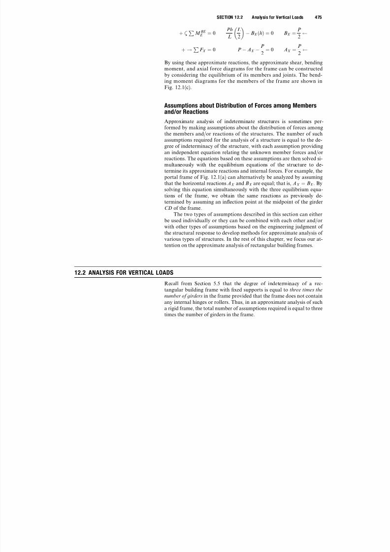
By using these approximate reactions, the approximate shear, bendingmoment, and axial force diagrams for the frame can be constructedby considering the equilibrium of its members and joints. The bend-ing moment diagrams for the members of the frame are shown inFig. 12.1(c).

Assumptions about Distribution of Forces among Membersand/or Reactions

Approximate analysis of indeterminate structures is sometimes per-formed by making assumptions about the distribution of forces amongthe members and/or reactions of the structures. The number of suchassumptions required for the analysis of a structure is equal to the de-gree of indeterminacy of the structure, with each assumption providingan independent equation relating the unknown member forces and/or

reactions. The equations based on these assumptions are then solved si-multaneously with the equilibrium equations of the structure to de-termine its approximate reactions and internal forces. For example, theportal frame of Fig. 12.1(a) can alternatively be analyzed by assumingthat the horizontal reactions AX and B X are equal; that is, AX ¼ B X . Bysolving this equation simultaneously with the three equilibrium equa-tions of the frame, we obtain the same reactions as previously de-termined by assuming an inflection point at the midpoint of the girder

CD of the frame.The two types of assumptions described in this section can eitherbe used individually or they can be combined with each other and/orwith other types of assumptions based on the engineering judgment of the structural response to develop methods for approximate analysis of various types of structures. In the rest of this chapter, we focus our at-tention on the approximate analysis of rectangular building frames.

12.2 ANALYSIS FOR VERTICAL LOADS

Recall from Section 5.5 that the degree of indeterminacy of a rec-tangular building frame with fixed supports is equal to three times the

number of girders in the frame provided that the frame does not containany internal hinges or rollers. Thus, in an approximate analysis of sucha rigid frame, the total number of assumptions required is equal to three

times the number of girders in the frame.

SECTION 12.2 Analysis for Vertical Loads 475



A commonly used procedure for approximate analysis of rec-tangular building frames subjected to vertical (gravity) loads involvesmaking three assumptions about the behavior of each girder of theframe. Consider a frame subjected to uniformly distributed loads w, as

shown in Fig. 12.2(a). The free-body diagram of a typical girder DE of the frame is shown in Fig. 12.2(b). From the deflected shape of thegirder sketched in the figure, we observe that two inflection points existnear both ends of the girder. These inflection points develop because thecolumns and the adjacent girder connected to the ends of girder DE of-fer partial restraint or resistance against rotation by exerting negativemoments M DE and M ED at the girder ends D and E , respectively. Al-though the exact location of the inflection points depends on the relative

sti¤nesses of the frame members and can be determined only from anexact analysis, we can establish the regions along the girder in whichthese points are located by examining the two extreme conditions of ro-tational restraint at the girder ends shown in Fig. 12.2(c) and (d). If thegirder ends were free to rotate, as in the case of a simply supportedgirder (Fig. 12.2(c)), the zero bending moments—and thus the inflectionpoints—would occur at the ends. On the other extreme, if the girderends were completely fixed against rotation, we can show by the exactanalysis presented in subsequent chapters that the inflection points

would occur at a distance of 0.211L from each end of the girder, as il-lustrated in Fig. 12.2(d). Therefore, when the girder ends are only par-tially restrained against rotation (Fig. 12.2(b)), the inflection points mustoccur somewhere within a distance of 0.211L from each end. Forthe purpose of approximate analysis, it is common practice to assumethat the inflection points are located about halfway between the twoextremes—that is, at a distance of 0.1L from each end of the girder.Estimating the location of two inflection points involves making two

assumptions about the behavior of the girder. The third assumption isbased on the experience gained from the exact analyses of rectangularframes subjected to vertical loads only, which indicates that the axialforces in girders of such frames are usually very small. Thus, in an ap-proximate analysis, it is reasonable to assume that the girder axial forcesare zero.

To summarize the foregoing discussion, in the approximate analysisof a rectangular frame subjected to vertical loads the following assump-tions are made for each girder of the frame:

1. The inflection points are located at one-tenth of the span from eachend of the girder.

2. The girder axial force is zero.

The e¤ect of these simplifying assumptions is that the middle eight-tenths of the span (0.8L) of each girder can be considered to be simplysupported on the two end portions of the girder, each of which isof the length equal to one-tenth of the girder span (0.1L), as shown in

Fig. 12.2(e). Note that the girders are now statically determinate, and




FIG. 12.2




FIG. 12.2 (contd.)




their end forces and moments can be determined from statics, as shownin the figure. It should be realized that by making three assumptionsabout the behavior of each girder of the frame, we have made a totalnumber of assumptions equal to the degree of indeterminacy of the

frame, thereby rendering the entire frame statically determinate, asshown in Fig. 12.2(f). Once the girder end forces have been computed,the end forces of the columns and the support reactions can be de-termined from equilibrium considerations.

Example 12.1

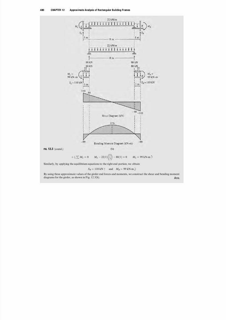
Draw the approximate shear and bending moment diagrams for the girders of the frame shown in Fig. 12.3(a).

Solution

As the span lengths and loads for the four girders of the frame are the same (Fig. 12.3(a)), the approximate shear andbending moment diagrams for the girders will also be the same. By applying the assumptions discussed in this section toany of the girders of the frame, we obtain the statically determinate girder shown in Fig. 12.3(b). Note that the middleportion of the girder, which has a length of 0:8L ¼ 0:8ð10Þ ¼ 8 m, is simply supported on the two end portions, each of length 0:1L ¼ 0:1ð10Þ ¼ 1 m

By considering the equilibrium of the simply supported middle portion of the girder, we obtain the vertical re-actions at the ends of this portion to be 22ð8=2Þ ¼ 88 kN. These forces are then applied in opposite directions(Newton’s law of action and reaction) to the two end portions, as shown in the figure. The vertical forces (shears) andmoments at the ends of the girder can now be determined by considering the equilibrium of the end portions. By ap-plying the equations of equilibrium to the left end portion, we write

þ "P

F Y ¼ 0 S L 22ð1Þ 88 ¼ 0 S L ¼ 110 kN "

continued

FIG. 12.3




þ ’P

M L ¼ 0 M L 22ð1Þ 1

2

88ð1Þ ¼ 0 M L ¼ 99 kN-m

’

Similarly, by applying the equilibrium equations to the right end portion, we obtain

S R ¼ 110 kN " and M R ¼ 99 kN-m @

By using these approximate values of the girder end forces and moments, we construct the shear and bending momentdiagrams for the girder, as shown in Fig. 12.3(b). Ans.

FIG. 12.3 (contd.)




12.3 ANALYSIS FOR LATERAL LOADS—PORTAL METHOD

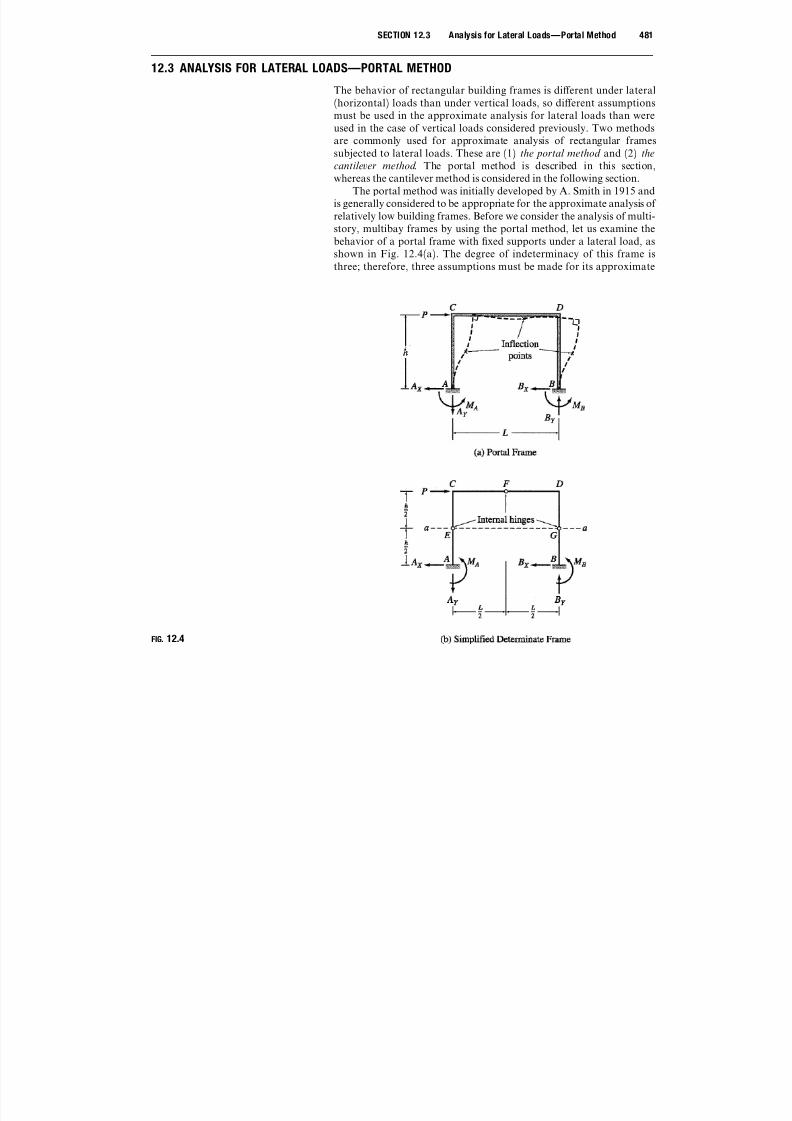
The behavior of rectangular building frames is di¤erent under lateral

(horizontal) loads than under vertical loads, so di¤erent assumptionsmust be used in the approximate analysis for lateral loads than wereused in the case of vertical loads considered previously. Two methodsare commonly used for approximate analysis of rectangular framessubjected to lateral loads. These are (1) the portal method and (2) the

cantilever method . The portal method is described in this section,whereas the cantilever method is considered in the following section.

The portal method was initially developed by A. Smith in 1915 andis generally considered to be appropriate for the approximate analysis of

relatively low building frames. Before we consider the analysis of multi-story, multibay frames by using the portal method, let us examine thebehavior of a portal frame with fixed supports under a lateral load, asshown in Fig. 12.4(a). The degree of indeterminacy of this frame isthree; therefore, three assumptions must be made for its approximate

FIG. 12.4

SECTION 12.3 Analysis for Lateral Loads—Portal Method 481



analysis. From the deflected shape of the frame sketched in Fig. 12.4(a),we observe that an inflection point exists near the middle of each mem-ber of the frame. Thus, in approximate analysis, it is reasonable to as-sume that the inflection points are located at the midpoints of the frame

members. Since the bending moments at the inflection points must bezero, internal hinges are inserted at the midpoints of the three framemembers to obtain the statically determinate frame shown in Fig.12.4(b). To determine the six reactions, we pass a horizontal section aa

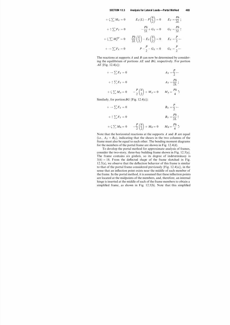
through the hinges E and G , as shown in Fig. 12.4(b), and apply theequations of equilibrium (and condition, if any) to the three portions of the frame. Applying the three equilibrium equations and one equationof condition to the portion ECDG (Fig. 12.4(c)), we compute the forces

at the internal hinges E and G to be

FIG. 12.4 (contd.)




þ ’P

M G ¼ 0 E Y ðLÞ P h

2

¼ 0 E Y ¼

Ph

2L#

þ "P F Y ¼ 0 Ph

2L

þ G Y ¼ 0 G Y ¼Ph

2L

"

þ ’P

M EF F ¼ 0

Ph

2L

L

2

E X

h

2

¼ 0 E X ¼

P

2

þ !P

F X ¼ 0 P P

2 G X ¼ 0 G X ¼

P

2

The reactions at supports A and B can now be determined by consider-

ing the equilibrium of portions AE and BG , respectively. For portionAE (Fig. 12.4(c)):

þ !P

F X ¼ 0 AX ¼P

2

þ "P

F Y ¼ 0 AY ¼Ph

2L#

þ’ P M

A ¼ 0

P

2

h

2

þM

A ¼ 0 M

A ¼

Ph

4

’

Similarly, for portion BG (Fig. 12.4(c)):

þ !P

F X ¼ 0 B X ¼P

2

þ "P

F Y ¼ 0 B Y ¼Ph

2L"

þ ’P

M B ¼ 0 P 2

h2

þ M B ¼ 0 M B ¼ Ph

4

’

Note that the horizontal reactions at the supports A and B are equal(i.e., AX ¼ B X ), indicating that the shears in the two columns of theframe must also be equal to each other. The bending moment diagramsfor the members of the portal frame are shown in Fig. 12.4(d).

To develop the portal method for approximate analysis of frames,consider the two-story, three-bay building frame shown in Fig. 12.5(a).

The frame contains six girders, so its degree of indeterminacy is3ð6Þ ¼ 18. From the deflected shape of the frame sketched in Fig.12.5(a), we observe that the deflection behavior of this frame is similarto that of the portal frame considered previously (Fig. 12.4(a)), in thesense that an inflection point exists near the middle of each member of the frame. In the portal method, it is assumed that these inflection pointsare located at the midpoints of the members, and, therefore, an internalhinge is inserted at the middle of each of the frame members to obtain a

simplified frame, as shown in Fig. 12.5(b). Note that this simplified




frame is not statically determinate because it is obtained by insertingonly 14 internal hinges (i.e., one hinge in each of the 14 members) into

the original frame, which is indeterminate to the 18th degree. Thus, thedegree of indeterminacy of the simplified frame of Fig. 12.5(b) is

FIG. 12.5




18 14 ¼ 4; therefore, four additional assumptions must be made be-fore an approximate analysis involving only statics can be carried out.In the portal method, it is further assumed that the frame is composedof a series of portal frames, as shown in Fig. 12.5(c), with each interior

column of the original multibay frame representing two portal legs. Weshowed previously (Fig. 12.4) that when a portal frame with internalhinges at the midpoints of its members is subjected to a lateral load,equal shears develop in the two legs of the portal. Since an interior col-umn of the original multibay frame represents two portal legs, whereasan exterior column represents only one leg, we can reasonably assumethat the shear in an interior column of a story of the multibay frame istwice as much as the shear in an exterior column of that story (Fig.

12.5(c)). The foregoing assumption regarding shear distribution betweencolumns yields one more equation for each story of the frame withmultiple bays than necessary for approximate analysis. For example, foreach story of the frame of Fig. 12.5, this assumption can be used to ex-press shears in any three of the columns in terms of that in the fourth.Thus, for the entire frame, this assumption provides a total of six equa-tions—that is, two equations more than necessary for approximateanalysis. However, as the extra equations are consistent with the rest,they do not cause any computational di‰culty in the analysis.

From the foregoing discussion, we gather that the assumptionsmade in the portal method are as follows:

1. An inflection point is located at the middle of each member of theframe.

2. On each story of the frame, interior columns carry twice as muchshear as exterior columns.

Procedure for Analysis

The following step-by-step procedure can be used for the approximateanalysis of building frames by the portal method.

1. Draw a sketch of the simplified frame obtained by inserting an in-ternal hinge at the midpoint of each member of the given frame.

2. Determine column shears. For each story of the frame:a. Pass a horizontal section through all the columns of the story,

cutting the frame into two portions.b. Assuming that the shears in interior columns are twice as much

as in exterior columns, determine the column shears by apply-ing the equation of horizontal equilibrium ð

PF X ¼ 0Þ to the

free body of the upper portion of the frame.3. Draw free-body diagrams of all the members and joints of the

frame, showing the external loads and the column end shears com-puted in the previous step.

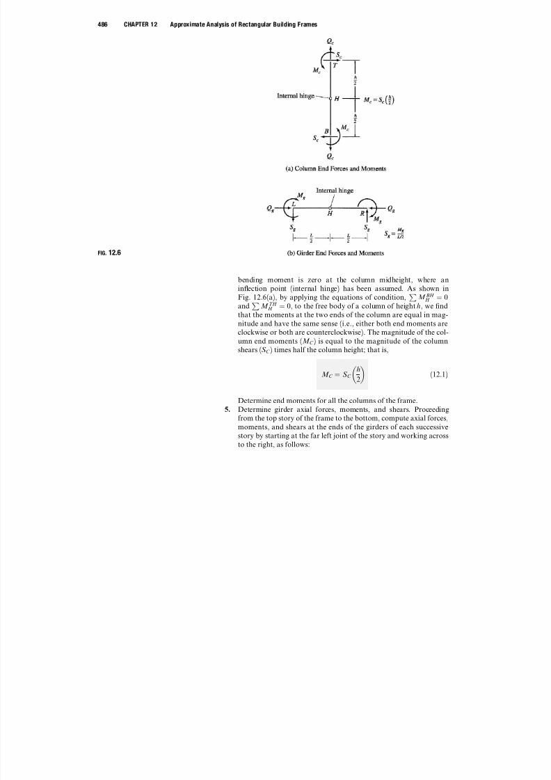
4. Determine column moments. Determine moments at the endsof each column by applying the equations of condition that the




bending moment is zero at the column midheight, where aninflection point (internal hinge) has been assumed. As shown in

Fig. 12.6(a), by applying the equations of condition,P

M BH

H ¼ 0and

PM TH

H ¼ 0, to the free body of a column of height h, we findthat the moments at the two ends of the column are equal in mag-nitude and have the same sense (i.e., either both end moments areclockwise or both are counterclockwise). The magnitude of the col-umn end moments (M C ) is equal to the magnitude of the columnshears (S C ) times half the column height; that is,

M C ¼ S C

h

2

(12.1)

Determine end moments for all the columns of the frame.5. Determine girder axial forces, moments, and shears. Proceeding

from the top story of the frame to the bottom, compute axial forces,moments, and shears at the ends of the girders of each successivestory by starting at the far left joint of the story and working across

to the right, as follows:

FIG. 12.6




a. Apply the equilibrium equations,P

F X ¼ 0 andP

M ¼ 0, tothe free body of the joint under consideration to compute theaxial force and moment, respectively, at the left (adjoining) endof the girder on the right side of the joint.

b. Considering the free body of the girder, determine the shear atthe girder’s left end by dividing the girder moment by half thegirder length (see Fig. 12.6(b)); that is,

S g ¼ M g

ðL=2Þ (12.2)

Equation (12.2) is based on the condition that the bending mo-ment at the girder midpoint is zero.

c. By applying the equilibrium equationsP

F X ¼ 0,P

F Y ¼ 0,and

PM ¼ 0 to the free body of the girder, determine the axial

force, shear, and moment, respectively, at the right end. Asshown in Fig. 12.6(b), the axial forces and shears at the ends of the girder must be equal but opposite, whereas the two endmoments must be equal to each other in both magnitude and

direction.d. Select the joint to the right of the girder considered previously,and repeat steps 5(a) through 5(c) until the axial forces, mo-ments, and shears in all the girders of the story have been de-termined. The equilibrium equations

PF X ¼ 0 and

PM ¼ 0

for the right end joint have not been utilized so far, so theseequations can be used to check the calculations.

e. Starting at the far left joint of the story below the one consid-ered previously, repeat steps 5(a) through 5(d) until the axial

forces, moments, and shears in all of the girders of the framehave been determined.

6. Determine column axial forces. Starting at the top story, apply theequilibrium equation

PF Y ¼ 0 successively to the free body of

each joint to determine the axial forces in the columns of the story.Repeat the procedure for each successive story, working from top tobottom, until the axial forces in all the columns of the frame havebeen determined.

7.

Realizing that the forces and moments at the lower ends of thebottom-story columns represent the support reactions, use the threeequilibrium equations of the entire frame to check the calculations.If the analysis has been performed correctly, then these equilibriumequations must be satisfied.

In steps 5 and 6 of the foregoing procedure, if we wish to computemember forces and moments by proceeding from the right end of thestory toward the left, then the term left should be replaced by right and

vice versa.




Example 12.2

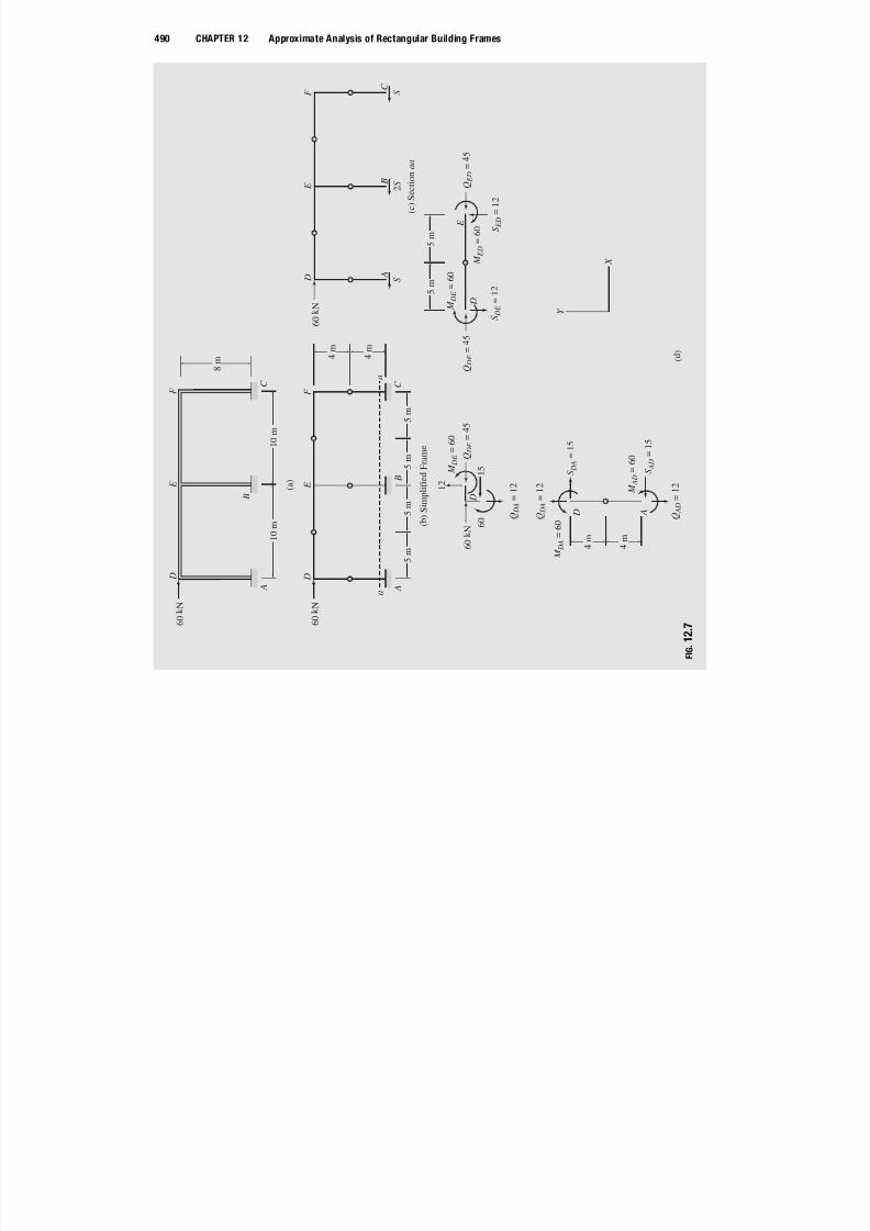
Determine the approximate axial forces, shears, and moments for all the members of the frame shown in Fig. 12.7(a) byusing the portal method.

Solution

Simplified Frame The simplified frame for approximate analysis is obtained by inserting internal hinges at themidpoints of all the members of the given frame, as shown in Fig. 12.7(b).

Column Shears To compute shears in the columns of the frame, we pass an imaginary section aa through thecolumns just above the support level, as shown in Fig. 12.7(b). The free-body diagram of the portion of the frame

above section aa is shown in Fig. 12.7(c). Note that the shear in the interior column BE has been assumed to be twiceas much as in the exterior columns AD and CF . By applying the equilibrium equation

PF X ¼ 0, we obtain (see

Fig. 12.7(c))

þ!P

F X ¼ 0 60 S 2S S ¼ 0 S ¼ 15 kN

Thus, the shear forces at the lower ends of the columns are

S AD ¼ S CF ¼ S ¼ 15 kN S BE ¼ 2S ¼ 30 kN

Shear forces at the upper ends of the columns are obtained by applying the equilibrium equationP

F X ¼ 0 to thefree body of each column. For example, from the free-body diagram of column AD shown in Fig. 12.7(d), we observethat in order to satisfy

PF X ¼ 0, the shear force at the upper end, S DA, must act to the right with a magnitude of 15 kN

to balance the shear force at the lower end, S AD ¼ 15 kN to the left. Thus, S DA ¼ 15 kN !. Shear forces at the upperends of the remaining columns are determined in a similar manner and are shown in Fig. 12.7(e), which depicts the free-body diagrams of all the members and joints of the frame.

Column Moments With the column shears now known, the column end moments can be computed by multiplyingthe column shears by half of the column heights. For example, since column AD (see Fig. 12.7(d)) is 8 m high and has

end shears of 15 kN, its end moments are

M AD ¼ M DA ¼ 15 8

2

¼ 60 kNm

’

Note that the end moments, M AD and M DA, are both counterclockwise—that is, opposite to the clockwise moments of the 15 kN end shears about the internal hinge at the column midheight. The end moments of the remaining columns of the frame are computed in a similar manner and are shown in Fig. 12.7(e).

Girder Axial Forces, Moments, and Shears We begin the calculation of girder end actions at the upper left jointD. The column shear S DA and moment M DA computed previously are applied to the free-body diagram of joint D

in opposite directions according to Newton’s third law, as shown in Fig. 12.7(d). By applying the equilibrium equationPF X ¼ 0, we obtain the girder axial force QDE ¼ 45 kN on joint D. Note that QDE must act in the opposite

direction—that is, to the right—at end D of girder DE . From the free-body diagram of joint D (Fig. 12.7(d)), we can

continued




also see that in order to satisfy the moment equilibrium equation, ðP

M ¼ 0Þ, the girder end moment M DE must beequal and opposite to the 60 kNm column end moment. Thus, M DE ¼ 60 kNm, with a counterclockwise direction

on joint D but a clockwise direction at the end D of girder DE .To evaluate the girder shear S DE , we consider the moment equilibrium of the left half of girder DE . From the free-

body diagram of girder DE in Fig. 12.7(d), we can see that the shear force S DE must act downward with a magnitude of M DE =ðL=2Þ so that it can develop a counterclockwise moment of magnitude, M DE , about the internal hinge to balancethe clockwise end moment, M DE . Thus,

S DE ¼ M DE

ðL=2Þ¼

60

ð10=2Þ¼ 12 kN #

The axial force, shear, and moment at the right end E can now be determined by applying the three equilibrium equa-tions to the free body of girder DE (Fig. 12.7(d)):

þ!P

F X ¼ 0 45 QED ¼ 0 QED ¼ 45 kN

þ "P

F Y ¼ 0 12 þ S ED ¼ 0 S ED ¼ 12 kN "

þ ’P

M D ¼ 0 60 M ED þ 12ð10Þ ¼ 0 M ED ¼ 60 kNm @

Note that the girder end moments, M DE and M ED, are equal in magnitude and have the same direction.Next, we calculate the end actions for girder EF . We first apply the equilibrium equations

PF X ¼ 0 and

PM ¼ 0

to the free body of joint E (Fig. 12.7(e)) to obtain the axial force QEF ¼ 15 kN ! and the moment M EF ¼60 kNm @ at the left end E of the girder. We then obtain the shear S EF ¼12 kN # by dividing the moment M EF byhalf of the girder length, and we apply the three equilibrium equations to the free body of the girder to obtain QFE ¼15 kN , S FE ¼ 12 kN ", and M FE ¼ 60 kNm @ at the right end F of the girder (see Fig. 12.7(e)).

Since all the moments and horizontal forces acting at the upper right joint F are now known, we can check thecalculations that have been performed thus far by applying the two equilibrium equations

PF X ¼ 0 and

PM ¼ 0 to

the free body of this joint. From the free-body diagram of joint F shown in Fig. 12.7(e), it is obvious that these equili-

brium equations are indeed satisfied.

Column Axial Forces We begin the calculation of column axial forces at the upper left joint D. From the free-bodydiagram of this joint shown in Fig. 12.7(d), we observe that the axial force in column AD must be equal and opposite tothe shear in girder DE . Thus, the axial force at the upper end D of column AD is QDA ¼ 12 kN ". By applyingP

F Y ¼ 0 to the free body of column AD, we obtain the axial force at the lower end A of the column to beQAD ¼ 12 kN #. Thus, the column AD is subjected to an axial tensile force of 12 kN. Axial forces for the remainingcolumns BE and CF are calculated similarly by considering the equilibrium of joints E and F , respectively. The axialforces thus obtained are shown in Fig. 12.7(e). Ans.

Reactions The forces and moments at the lower ends of the columns AD; BE , and CF , represent the reactions atthe fixed supports A; B , and C , respectively, as shown in Fig. 12.7(f). Ans.

continued


490 CHAPTER 12 A i t A l i f R t l B ildi F



1 0 m

1 0 m

( a )

8 m

A

C

B

D

E

F

6 0 k N

5 m

5 m

5 m

5 m

( b ) S i m p l i f i e d

F r a m e

4

m 4

m

A

C

B

D

E

F

6 0 k N

a

a

( c ) S e c t i o n a a

A S

2 S

S

B

C

D

E

F

6 0 k N

5 m

5 m

M D E = 6 0

Q D E

= 4 5

Q D E = 4 5

Q E D = 4 5

D

E

S D E = 1 2

S E D = 1 2

M E D =

6 0

X

Y

6 0 k N

1 2 M

D E = 6 0

1

5

6 0

D

Q D A = 1 2

Q D A = 1 2

Q A D = 1 2

4

m 4

m

M D A = 6 0

S

D A = 1 5

M A D = 6 0

S

A D = 1 5

A D

( d

)

F I G .

1 2 . 7


SECTION 12 3 Analysis for Lateral Loads Portal Method 491



D

E

F C

6 0 6

0

6 0

1 2

1 5

1 2

4 5

4 5

1 5

1 5

1 5

4 5

6 0

6 0

6 0

6 0

1 2

1 2

1 2

1 2

6 0

1 2

1 5

6 0

6 0 1 5

1 2

6 0

6 0

6 0

3 0

4 5

1 5

1 2

1 2

1 2

1 2 0

1 5

B 1 2 0

3 0

1 2

0

( e ) M e m b e r E n d

F o r c e s

a n d

M o m e n t s

3 0

1 5

1 5

6 0

6 0

1 2

1 2

A

1 2

A

C

B

D

E

F

6 0 k N

1 5

6 0

1 2

( f ) S u p p o r t R e a c

t i o n s

3 0

1 2 0

1 5

6 0

1 2

F I G .

1 2 . 7

( c o n t d . )





FIG. 12.8

Checking Computations To check our computations, we apply the three equilibrium equations to the free body of the entire frame (Fig. 12.7(f)):

þ!P

F X ¼ 0 60 15 30 15 ¼ 0 Checks

þ "P

F Y ¼ 0 12 þ 12 ¼ 0 Checks

þ ’P

M C ¼ 0 60ð8Þ þ 12ð20Þ þ 60 þ 120 þ 60 ¼ 0 Checks

Example 12.3

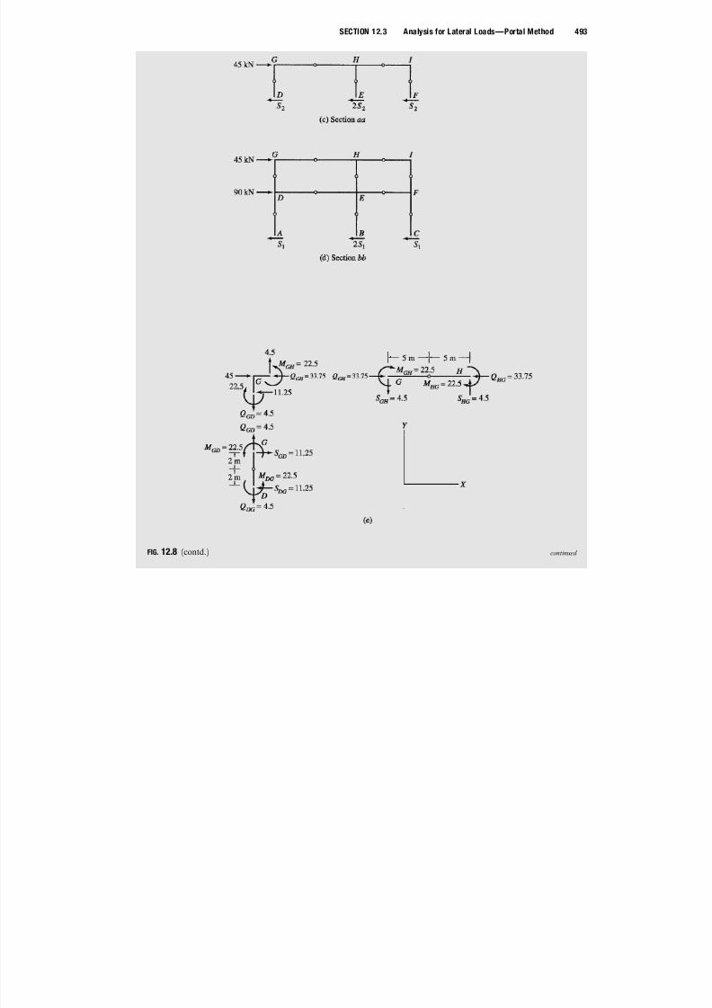
Determine the approximate axial forces, shears, and moments for all the members of the frame shown in Fig. 12.8(a) byusing the portal method.

Solution

Simplified Frame The simplified frame is obtained by inserting internal hinges at the midpoints of all the membersof the given frame, as shown in Fig. 12.8(b).

Column Shears To compute shears in the columns of the second story of the frame, we pass an imaginary sectionaa through the columns DG ; EH , and FI just above the floor level, as shown in Fig. 12.8(b). The free-body diagram of the portion of the frame above section aa is shown in Fig. 12.8(c). Note that the shear in the interior column EH hasbeen assumed to be twice as much as in the exterior columns DG and FI . By applying the equilibrium equationP

F X ¼ 0, we obtain (Fig. 12.8(c))

þ!P

F X ¼ 0 45 S 2 2S 2 S 2 ¼ 0 S 2 ¼ 11:25 kN

continued





FIG. 12.8 (contd.) continued

SECTION 12.3 Analysis for Lateral Loads Portal Method 493




F I G .

1 2 . 8

( c o n t d . )

pp y g g




Thus, the shear forces at the lower ends of the second-story columns are

S DG ¼ S FI ¼ S 2 ¼ 11:25 kN S EH ¼ 2S 2 ¼ 22:5 kN

Similarly, by employing section bb (Fig. 12.8(b)), we determine shear forces at the lower ends of the first-storycolumns AD; BE , and CF to be (see Fig. 12.8(d)):

S AD ¼ S CF ¼ S 1 ¼ 33:75 kN S BE ¼ 2S 1 ¼ 67:5 kN

Shear forces at the upper ends of columns are determined by applying the equilibrium equationP

F X ¼ 0 to thefree body of each column. For example, from the free-body diagram of column DG shown in Fig. 12.8(e), we can seethat in order to satisfy

PF X ¼ 0, the shear force at the upper end, S GD, must act to the right with a magnitude of

11.25 kN. Thus S GD ¼ 11:25 kN !. Shear forces at the upper ends of the remaining columns are obtained in a similarmanner and are shown in Fig. 12.8(f), which depicts the free-body diagrams of all the members and joints of the frame.

Column Moments Knowing column shears, we can now compute the column end moments by multiplying thecolumn shears by half of the column heights. For example, since column DG (see Fig. 12.8(e)) is 4 m high and has endshears of 11.25 kN, its end moments are

M DG ¼ M GD ¼ 11:25 4 m

2

¼ 22:5 kNm

’

Note that the end moments, M DG and M GD, are both counterclockwise—that is, opposite to the clockwise moments of the 11.25 kN end shears about the internal hinge at the column midheight. The end moments of the remaining columnsare computed in a similar manner and are shown in Fig. 12.8(f).

Girder Axial Forces, Moments, and Shears We begin the computation of girder end actions at the upper left joint G .The column shear S GD and moment M GD computed previously are applied to the free-body diagram of joint G in op-posite directions in accordance with Newton’s third law, as shown in Fig. 12.8(e). By summing forces in the horizontal

FIG. 12.8 (contd.)

continued




direction, we obtain the girder axial force QGH ¼ 33:75 kN on joint G . Note that QGH must act in the opposite di-rection—that is, to the right—at the end G of girder GH . From the free-body diagram of joint G (Fig. 12.8(e)), we canalso see that in order to satisfy the moment equilibrium ðPM ¼ 0Þ, the girder end moment M GH must be equal and

opposite to the 22.5 kN-m column end moment. Thus M GH ¼ 22:5 kN-m, with a counterclockwise direction on joint G but a clockwise direction at the end G of girder GH .

To determine the girder shear S GH , we consider the moment equilibrium of the left half of girder GH . From thefree-body diagram of girder GH (Fig. 12.8(e)), we can see that the shear force S GH must act downward with a magni-tude of M GH =ðL=2Þ so that it can develop a counterclockwise moment of magnitude M GH about the internal hinge tobalance the clockwise end moment M GH . Thus

S GH ¼ M GH

ðL=2Þ¼

22:5

ð10=2Þ¼ 4:5 kN #

The axial force, shear, and moment at the right end H can now be computed by applying the three equilibrium equa-tions to the free body of girder GH (Fig. 12.8(e)). Applying

PF X ¼ 0, we obtain QHG ¼ 33:75 kN . From

PF Y ¼ 0,

we obtain S HG ¼ 1 k ", and to compute M HG , we apply the equilibrium equation:

þ ’P

M G ¼ 0 22:5 M HG þ 4:5ð10Þ ¼ 0 M HG ¼ 22:5 kN-m @

Note that the girder end moments, M GH and M HG , are equal in magnitude and have the same direction.Next, the end actions for girder HI are computed. The equilibrium equations

PF X ¼ 0 and

PM ¼ 0

are first applied to the free body of joint H (Fig. 12.8(f)) to obtain the axial force QHI ¼ 11:25 kN ! and the

moment M HI ¼22:5 kN-m @ at the left end H of the girder. The shear S HI ¼ 7:5 kN # is then obtained by dividingthe moment M HI by half the girder length, and the three equilibrium equations are applied to the free body of the girder to obtain QIH ¼ 11:25 kN , S IH ¼ 7:5 kN ", and M IH ¼ 22:5 kN-m @ at the right end I of the girder(see Fig. 12.8(f)).

All the moments and horizontal forces acting at the upper right joint I are now known, so we cancheck the calculations performed thus far by applying

PF X ¼ 0 and

PM ¼ 0 to the free body of this joint.

From the free-body diagram of joint I shown in Fig. 12.8(f), it is obvious that these equilibrium equations are indeedsatisfied.

The end actions for the first-story girders DE and EF are computed in a similar manner, by starting at the left jointD and working across to the right. The girder end actions thus obtained are shown in Fig. 12.8(f).

Column Axial Forces We begin the computation of column axial forces at the upper left joint G . From thefree-body diagram of joint G shown in Fig. 12.8(e), we observe that the axial force in column DG must be equaland opposite to the shear in girder GH . Thus the axial force at the upper end G of column DG isQGD ¼ 4:5 kN ". By applying

PF Y ¼ 0 to the free body of column DG , we obtain the axial force at the lower

end of the column to be QDG ¼ 4:5 kN #. Thus, the column DG is subjected to an axial tensile force of 4.5 kN.Axial forces for the remaining second-story columns, EH and FI , are determined similarly by considering theequilibrium of joints H and I , respectively; thereafter, the axial forces for the first-story columns, AD; BE , andCF , are computed from the equilibrium consideration of joints D; E , and F , respectively. The axial forces thus

obtained are shown in Fig. 12.8(f). Ans.

Reactions The forces and moments at the lower ends of the first-story columns AD; BE , and CF , represent the re-actions at the fixed supports A; B , and C , respectively, as shown in Fig. 12.8(g). Ans.

continued

SECTION 12.4 Analysis for Lateral Loads—Cantilever Method 497



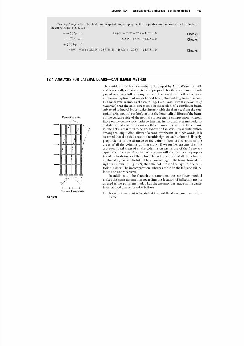
12.4 ANALYSIS FOR LATERAL LOADS—CANTILEVER METHOD

The cantilever method was initially developed by A. C. Wilson in 1908and is generally considered to be appropriate for the approximate anal-ysis of relatively tall building frames. The cantilever method is basedon the assumption that under lateral loads, the building frames behave

like cantilever beams, as shown in Fig. 12.9. Recall (from mechanics of materials) that the axial stress on a cross section of a cantilever beamsubjected to lateral loads varies linearly with the distance from the cen-troidal axis (neutral surface), so that the longitudinal fibers of the beamon the concave side of the neutral surface are in compression, whereasthose on the convex side undergo tension. In the cantilever method, thedistribution of axial stress among the columns of a frame at the columnmidheights is assumed to be analogous to the axial stress distribution

among the longitudinal fibers of a cantilever beam. In other words, it isassumed that the axial stress at the midheight of each column is linearlyproportional to the distance of the column from the centroid of theareas of all the columns on that story. If we further assume that thecross-sectional areas of all the columns on each story of the frame areequal, then the axial force in each column will also be linearly propor-tional to the distance of the column from the centroid of all the columnson that story. When the lateral loads are acting on the frame toward theright, as shown in Fig. 12.9, then the columns to the right of the cen-troidal axis will be in compression, whereas those on the left side will bein tension and vice versa.

In addition to the foregoing assumption, the cantilever methodmakes the same assumption regarding the location of inflection pointsas used in the portal method. Thus the assumptions made in the canti-lever method can be stated as follows:

1. An inflection point is located at the middle of each member of theframe.FIG. 12.9

Checking Computations To check our computations, we apply the three equilibrium equations to the free body of the entire frame (Fig. 12.8(g)):

þ!PF

X ¼ 0 45 þ 90 33:75 67:5 33:75 ¼ 0 Checksþ "

PF Y ¼ 0 22:875 17:25 þ 43:125 ¼ 0 Checks

þ ’P

M C ¼ 0

45ð9Þ 90ð5Þ þ 84:375 þ 25:875ð16Þ þ 168:75 þ 17:25ð6Þ þ 84:375 ¼ 0 Checks




2. On each story of the frame, the axial forces in columns are linearlyproportional to their distances from the centroid of the cross-sectional areas of all the columns on that story.

Procedure for Analysis

The following step-by-step procedure can be used for the approximateanalysis of building frames by the cantilever method.

1. Draw a sketch of the simplified frame obtained by inserting an in-ternal hinge at the midpoint of each member of the given frame.

2. Determine column axial forces. For each story of the frame:

a. Pass a horizontal section through the internal hinges at the col-umn midheights, cutting the frame into two portions.

b. Draw a free-body diagram of the portion of the frame abovethe section. Because the section passes through the columns atthe internal hinges, only internal shears and axial forces (but nointernal moments) act on the free body at the points where thecolumns have been cut.

c. Determine the location of the centroid of all the columns on thestory under consideration.

d. Assuming that the axial forces in the columns are proportionalto their distances from the centroid, determine the columnaxial forces by applying the moment equilibrium equation,P

M ¼ 0, to the free body of the frame above the section. Toeliminate the unknown column shears from the equilibriumequation, the moments should be summed about one of the in-ternal hinges at the column midheights through which the sec-tion has been passed.

3. Draw free-body diagrams of all the members and joints of the frameshowing the external loads and the column axial forces computed inthe previous step.

4. Determine girder shears and moments. For each story of the frame,the shears and moments at the ends of girders are computed bystarting at the far left joint and working across to the right (or viceversa), as follows:a. Apply the equilibrium equation

PF Y ¼ 0 to the free body of

the joint under consideration to compute the shear at the leftend of the girder that is on the right side of the joint.b. Considering the free body of the girder, determine the moment

at the girder’s left end by multiplying the girder shear by half the girder length; that is,

M g ¼ S gL

2

(12.3)




Equation (12.3) is based on the condition that the bending mo-ment at the girder midpoint is zero.

c. By applying the equilibrium equationsP

F Y ¼ 0 andP

M ¼ 0to the free body of the girder, determine the shear and moment,

respectively, at the right end.d. Select the joint to the right of the girder considered previously,

and repeat steps 4(a) through 4(c) until the shears and momentsin all the girders of the story have been determined. Because theequilibrium equation

PF Y ¼ 0 for the right end joint has not

been utilized so far, it can be used to check the calculations.5. Determine column moments and shears. Starting at the top story,

apply the equilibrium equationP

M ¼ 0 to the free body of each joint of the story to determine the moment at the upper end of the

column below the joint. Next, for each column of the story, calcu-late the shear at the upper end of the column by dividing the col-umn moment by half the column height; that is,

S C ¼ M C

ðh=2Þ (12.4)

Determine the shear and moment at the lower end of the columnby applying the equilibrium equationsP

F X ¼ 0 andP

M ¼ 0, re-spectively, to the free body of the column. Repeat the procedure foreach successive story, working from top to bottom, until the mo-ments and shears in all the columns of the frame have been de-termined.

6. Determine girder axial forces. For each story of the frame, de-termine the girder axial forces by starting at the far left joint andapplying the equilibrium equation P F X ¼ 0 successively to the free

body of each joint of the story.7. Realizing that the forces and moments at the lower ends of the

bottom-story columns represent the support reactions, use the threeequilibrium equations of the entire frame to check the calculations.If the analysis has been performed correctly, then these equilibriumequations must be satisfied.

Example 12.4

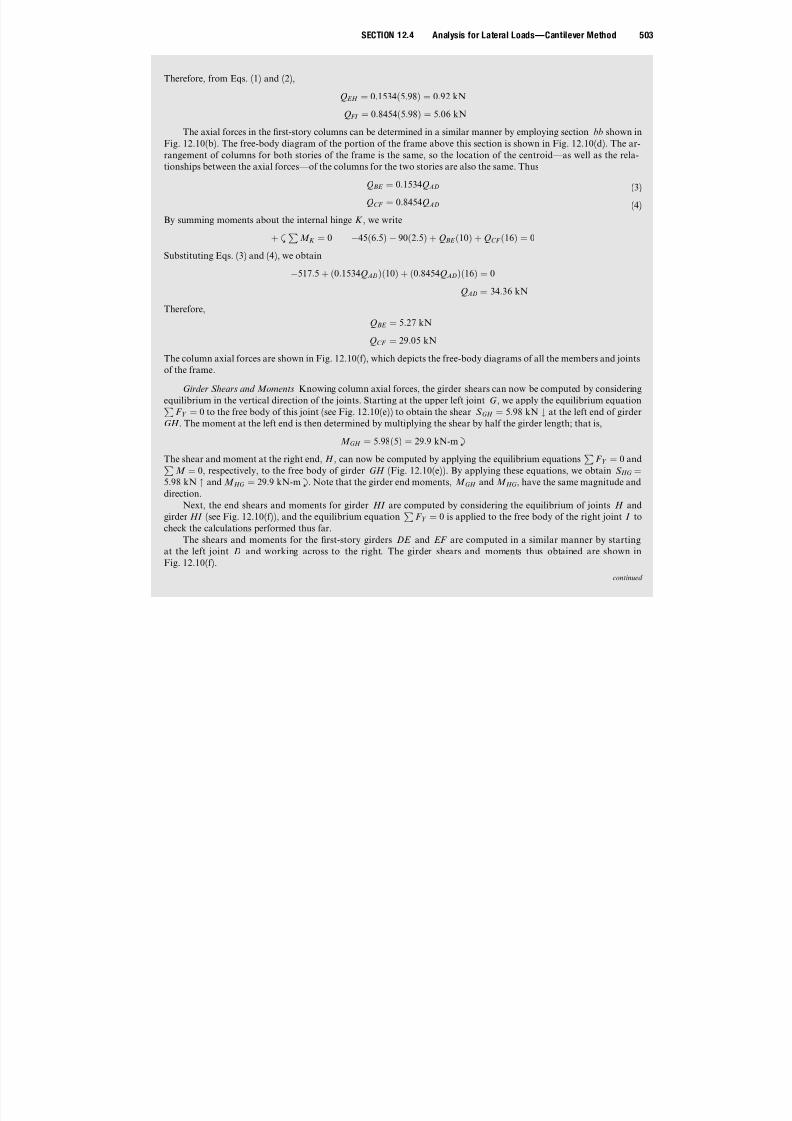
Determine the approximate axial forces, shears, and moments for all the members of the frame shown in Fig. 12.10(a)by using the cantilever method.

Solution

This frame was analyzed by the portal method in Example 12.3. continued




FIG. 12.10continued




F I G .

1 2 . 1

0

( c o n t d . )




Simplified Frame The simplified frame, obtained by inserting internal hinges at midpoints of all the members of thegiven frame, is shown in Fig. 12.10(b).

Column Axial Forces To compute axial forces in the columns of the second story of the frame, we pass an imagi-nary section aa through the internal hinges at the midheights of columns DG ; EH , and FI , as shown in Fig. 12.10(b).The free-body diagram of the portion of the frame above this section is shown in Fig. 12.10(c). Because the section cutsthe columns at the internal hinges, only internal shears and axial forces (but no internal moments) act on the free bodyat the points where the columns have been cut. Assuming that the cross-sectional areas of the columns are equal, wedetermine the location of the centroid of the three columns from the left column DG by using the relationship

x ¼

PAxPA ¼

Að0Þ þAð10Þ þ Að16Þ

3A ¼ 8:67 m

The lateral loads are acting on the frame to the right, so the axial force in column DG , which is to the left of the cent-roid, must be tensile, whereas the axial forces in the columns EH and FI , located to the right of the centroid, must becompressive as shown in Fig. 12.10(c). Also, since the axial forces in the columns are assumed to be linearly propor-tional to their distances from the centroid, the relationships between them can be established by means of the similartriangles shown in Fig. 12.10(c); that is,

QEH ¼1:33

8:67QDG ¼ 0:1534QDG (1)

QFI ¼7:33

8:67QDG ¼ 0:8454QDG (2)

By summing moments about the left internal hinge J , we write

þ ’P

M J ¼ 0 45ð2Þ þ QEH ð10Þ þQFI ð16Þ ¼ 0

Substituting Eqs. (1) and (2) into the preceding equation and solving for QDG , we obtain

90 þ ð0:1534QDG Þð10Þ þ ð0:8454QDG Þð16Þ ¼ 0

QDG ¼ 5:98 kN

FIG. 12.10 (contd.)

continued




Therefore, from Eqs. (1) and (2),

QEH ¼ 0:1534ð5:98Þ ¼ 0:92 kN

QFI ¼ 0:8454ð5:98Þ ¼ 5:06 kN

The axial forces in the first-story columns can be determined in a similar manner by employing section bb shown inFig. 12.10(b). The free-body diagram of the portion of the frame above this section is shown in Fig. 12.10(d). The ar-rangement of columns for both stories of the frame is the same, so the location of the centroid—as well as the rela-tionships between the axial forces—of the columns for the two stories are also the same. Thus

QBE ¼ 0:1534QAD (3)

QCF ¼ 0:8454QAD (4)

By summing moments about the internal hinge K , we write

þ ’P

M K ¼ 0 45ð6:5Þ 90ð2:5Þ þ QBE ð10Þ þ QCF ð16Þ ¼ 0

Substituting Eqs. (3) and (4), we obtain

517:5 þ ð0:1534QADÞð10Þ þ ð0:8454QADÞð16Þ ¼ 0

QAD ¼ 34:36 kN

Therefore,

QBE ¼ 5:27 kN

QCF ¼ 29:05 kN

The column axial forces are shown in Fig. 12.10(f), which depicts the free-body diagrams of all the members and jointsof the frame.

Girder Shears and Moments Knowing column axial forces, the girder shears can now be computed by consideringequilibrium in the vertical direction of the joints. Starting at the upper left joint G , we apply the equilibrium equationP

F Y ¼ 0 to the free body of this joint (see Fig. 12.10(e)) to obtain the shear S GH ¼ 5:98 kN # at the left end of girderGH . The moment at the left end is then determined by multiplying the shear by half the girder length; that is,

M GH ¼ 5:98ð5Þ ¼ 29:9 kN-m @

The shear and moment at the right end, H , can now be computed by applying the equilibrium equationsP

F Y ¼ 0 andPM ¼ 0, respectively, to the free body of girder GH (Fig. 12.10(e)). By applying these equations, we obtain S HG ¼

5:98 kN " and M HG ¼ 29:9 kN-m @. Note that the girder end moments, M GH and M HG , have the same magnitude anddirection.

Next, the end shears and moments for girder HI are computed by considering the equilibrium of joints H andgirder HI (see Fig. 12.10(f)), and the equilibrium equation

PF Y ¼ 0 is applied to the free body of the right joint I to

check the calculations performed thus far.

The shears and moments for the first-story girders DE and EF are computed in a similar manner by startingat the left joint D and working across to the right. The girder shears and moments thus obtained are shown inFig. 12.10(f).

continued




SUMMARY

In this chapter, we have learned that in the approximate analysis of statically indeterminate structures, two types of simplifying assumptionsare commonly employed: (1) assumptions about the location of in-flection points and (2) assumptions about the distribution of forcesamong members and/or reactions. The total number of assumptions re-quired is equal to the degree of indeterminacy of the structure.

Column Moments and Shears With the girder moments now known, the column moments can be determined byconsidering moment equilibrium of joints. Beginning at the second story and applying

PM ¼ 0 to the free body of

joint G (Fig. 12.10(e)), we obtain the moment at the upper end of column DG to be M GD ¼ 29:9 kN-m ’

. The shear at

the upper end of column DG is then computed by dividing M GD by half the column height; that is,

S GD ¼29:9

2 ¼ 14:95 kN !

Note that S GD must act to the right, so that it can develop a clockwise moment to balance the counterclockwise endmoment M GD. The shear and moment at the lower end D are then determined by applying the equilibrium equationsP

F X ¼0 andP

M ¼ 0 to the free body of column DG (see Fig. 12.10(e)). Next, the end moments and shears for col-umns EH and FI are computed in a similar manner; thereafter, the procedure is repeated to determine the moments andshears for the first-story columns, AD; BE , and CF (see Fig. 12.10(f)).

Girder Axial Forces We begin the computation of girder axial forces at the upper left joint G . ApplyingP

F X ¼ 0to the free-body diagram of joint G shown in Fig. 12.10(e), we find the axial force in girder GH to be 30.05 kN com-pression. The axial force for girder HI is determined similarly by considering the equilibrium of joint H , after which theequilibrium equation

PF X ¼ 0 is applied to the free body of the right joint I to check the calculations. The axial forces

for the first-story girders DE and EF are then computed from the equilibrium consideration of joints D and E , in order.The axial forces thus obtained are shown in Fig. 12.10(f). Ans.

Reactions The forces and moments at the lower ends of the first-story columns AD; BE , and CF represent the re-actions at the fixed supports A; B , and C , respectively, as shown in Fig. 12.10(g). Ans.

Checking Computations To check our computations, we apply the three equilibrium equations to the free body of the entire frame (Fig. 12.10(g)):

þ !P

F X ¼ 0 45 þ 90 44:8 67:43 22:77 ¼ 0 Checks

þ "P

F Y ¼ 0 34:36 þ 5:27 þ 29:05 ¼ 0:04&0 Checks

þ ’P

M C ¼ 0

45ð9Þ 90ð5Þ þ 112 þ 34:36ð16Þ þ 168:575 5:27ð6Þ þ 56:93 ¼ 0:645&0

Checks

Th a i at a al i f ta la f a bj t d t ti

Problems 505



The approximate analysis of rectangular frames subjected to verti-cal loads is based on the following assumptions for each girder of theframe: (1) the inflection points are located at one-tenth of the span fromeach end of the girder and (2) the girder axial force is zero.

Two methods commonly used for the approximate analysis of rec-tangular frames subjected to lateral loads are the portal method and thecantilever method.

The portal method involves making the assumptions that an in-flection point is located at the middle of each member and that, oneach story, interior columns carry twice as much shear as exteriorcolumns.

In the cantilever method, the following assumptions are made aboutthe behavior of the frame: that an inflection point is located at the mid-

dle of each member and that, on each story, the axial forces in the col-umns are linearly proportional to their distances from the centroid of the cross-sectional areas of all the columns on that story.

PROBLEMSSection 12.2

12.1 through 12.5 Draw the approximate shear and bend-ing moment diagrams for the girders of the frames shown inFigs. P12.1 through P12.5.

30 k N/m

A

D

B

E

C

F

6 m 6 m

4 m

FIG. P12.1

15 k N/m

15 k N/m

5 m

A B

C D

E F

5 m

5 m

FIG. P12.2

Section 12 3




FIG. P12.3

30 k N/m

30 k N/m

6 m6 m

3 m

3 m

G

D

A B

E F

H

C

I

FIG. P12.4

12 m8 m

8 m

8 m

10 k N/m

20 k N/m

G

D

I

F

A

H

E

B C

FIG. P12.5

Section 12.3

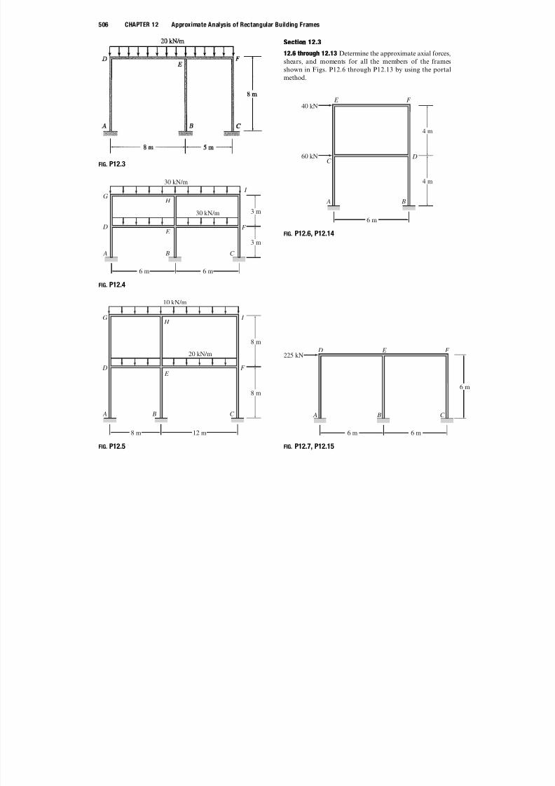
12.6 through 12.13 Determine the approximate axial forces,shears, and moments for all the members of the framesshown in Figs. P12.6 through P12.13 by using the portal

method.

6 m

4 m

4 m

40 k N

60 k N

A B

C

E F

D

FIG. P12.6, P12.14

A B

D E F

C

6 m 6 m

6 m

225 k N

FIG. P12.7, P12.15

Problems 507



FIG. P12.8, P12.16

FIG. P12.9, P12.17

10 m10 m

80 k N

40 k N

6 m

6 m

G

D

A B C

E F

H

C

I

FIG. P12.10, P12.18

FIG. P12.11, P12.19

FIG. P12.12, P12.20

FIG. P12.13, P12.21

Section 12.4

12.14 through 12.21 Determine the approximate axialforces, shears, and moments for all the members of theframes shown in Figs. P12.6 through P12.13 by using thecantilever method.

Structural Analysis Bab 12

Documents

Transcript of Structural Analysis Bab 12