STAT 515 fa 2021 Lec 12 slides Conﬁdence interval for the ...

STAT 515 fa 2021 Lec 12 slides

Confidence interval for the mean when variance unknown

Karl B. Gregory

University of South Carolina

These slides are an instructional aid; their sole purpose is to display, during the lecture,definitions, plots, results, etc. which take too much time to write by hand on the blackboard.

They are not intended to explain or expound on any material.

Karl B. Gregory (U. of South Carolina) STAT 515 fa 2021 Lec 12 slides 1 / 10

Recall: If X1, . . . ,Xnind⇠ Normal(µ,�2), then

X̄n ± z↵/2�pn

is a (1 � ↵)⇥ 100% CI for µ.

But what if we don’t know �?

Using X̄n ± z↵/2Sn/pn is okay if n is large, but not if n is small. . .


Twith Sn

SE E E x

OI estimator of E

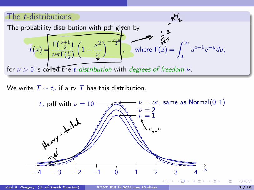
The t-distributionsThe probability distribution with pdf given by

f (x) =�( ⌫+1

2 )

⌫⇡�( ⌫2 )

✓1 +

x2

⌫

◆� ⌫+12

, where �(z) =

Z 1

0uz�1e�udu,

for ⌫ > 0 is called the t-distribution with degrees of freedom ⌫.

We write T ⇠ t⌫ if a rv T has this distribution.

⌫ = 1, same as Normal(0, 1)

⌫ = 1⌫ = 2

t⌫ pdf with ⌫ = 10

0�1 1 2�2 3�3 4�4 x


g

yayt T.nu

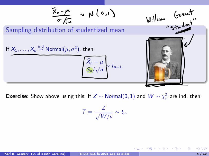
Sampling distribution of studentized mean

If X1, . . . ,Xnind⇠ Normal(µ,�2), then

X̄n � µ

Sn/pn⇠ tn�1.

Exercise: Show above using this: If Z ⇠ Normal(0, 1) and W ⇠ �2⌫ are ind. then

T =ZpW /⌫

⇠ t⌫ .


Fj N 0,1Willi

SÜß

Oh

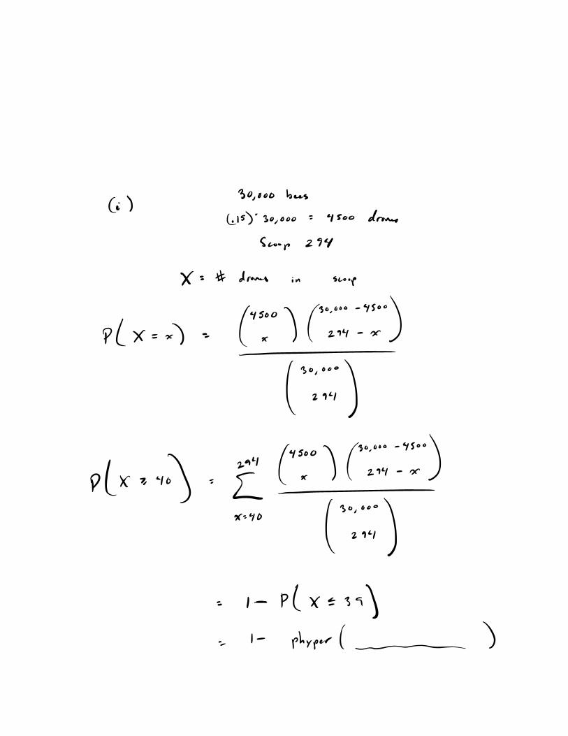
i30,000 bees

15 30,000 4500 dran

Scoop 294

X drums in scoop

plx n.li E294

294 xPlo Elif

X 40

I P X 3

I phyper

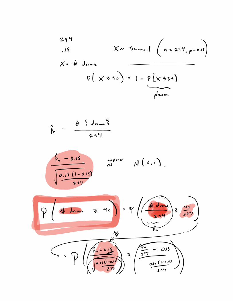
294

IS

X dran

mi n 294 p o

PIX D

in 42

t.ITi wco.n

P dem 4 P E

Fino

00

P LEID

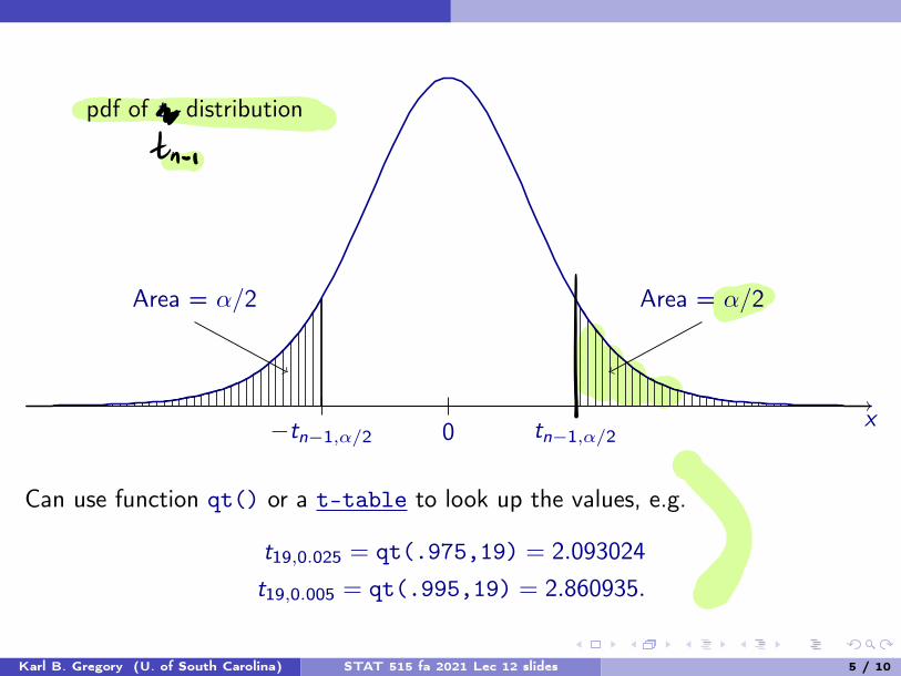
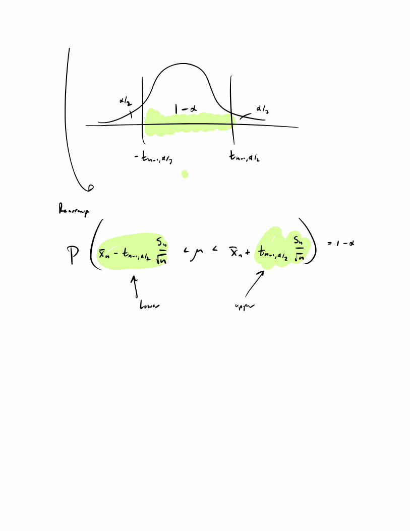
0 tn�1,↵/2

Area = ↵/2

�tn�1,↵/2

Area = ↵/2

pdf of t⌫ distribution

x

Can use function qt() or a t-table to look up the values, e.g.

t19,0.025 = qt(.975,19) = 2.093024t19,0.005 = qt(.995,19) = 2.860935.


Ä

https://people.stat.sc.edu/gregorkb/t-table.pdf

Confidence interval for mean of a Normal population with � unknown

Let X1, . . . ,Xnind⇠ Normal(µ,�2). Then a (1 � ↵)⇥ 100% CI for µ is

X̄n ± tn�1,↵/2Snpn.

Show where this CI comes from.


In Zu

According to Gossett

Etna FEEin

tA

Rearrange

P n tun En n F tun

9Lower upper

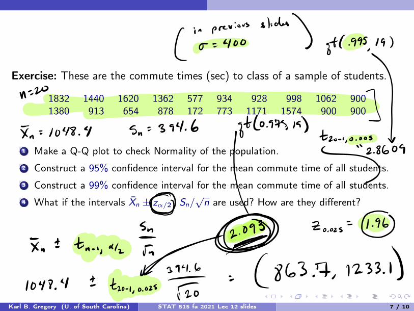
Exercise: These are the commute times (sec) to class of a sample of students.

1832 1440 1620 1362 577 934 928 998 1062 900

1380 913 654 878 172 773 1171 1574 900 900

1 Make a Q-Q plot to check Normality of the population.

2 Construct a 95% confidence interval for the mean commute time of all students.

3 Construct a 99% confidence interval for the mean commute time of all students.

4 What if the intervals X̄n ± z↵/2 · Sn/pn are used? How are they different?


ä gc.ass.is

n O

In 1048 4 5 394.6

4.974 tuj.E CZ

863.7 1233.11048.4

Mean weight of 2 cup up flow scooped

In 153.2857 n 21

Sn 18.892

A sst I tuµ

is

153.2857 tz 1 0.02s HÄ27086 flo 975,20

44.69 161.89

tnn.az got 4 n

Ina als

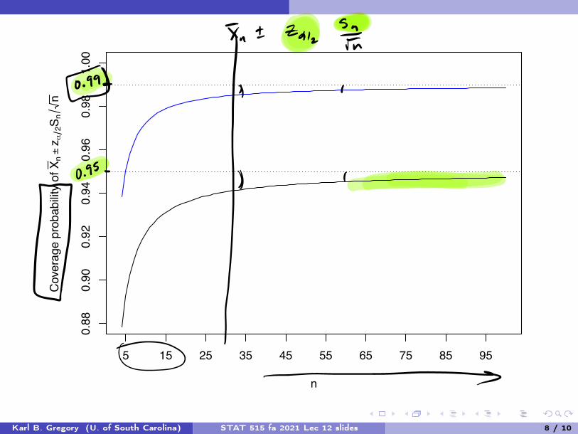
0.88

0.90

0.92

0.94

0.96

0.98

1.00

n

Cov

erag

e pr

obab

ility

of X

n±

z α2S

nn

5 15 25 35 45 55 65 75 85 95


In Zu Er

ß

I

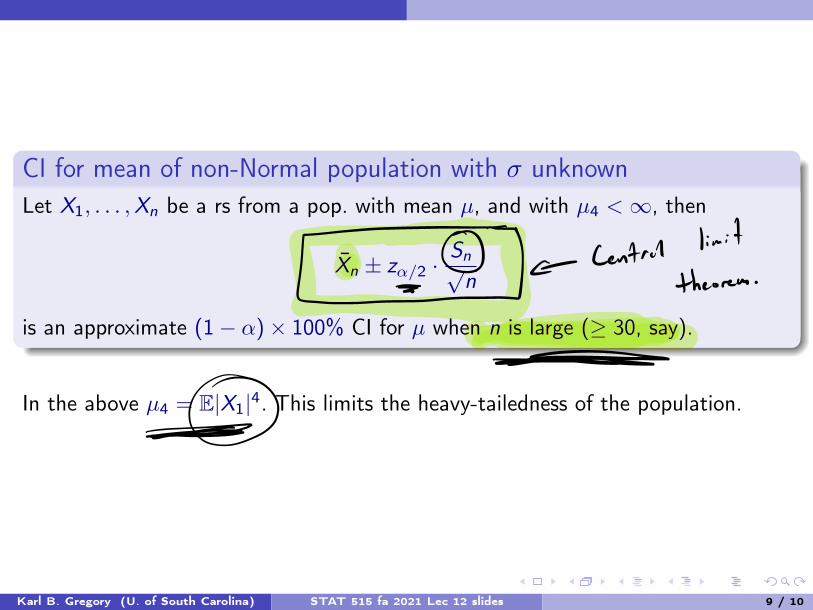
CI for mean of non-Normal population with � unknownLet X1, . . . ,Xn be a rs from a pop. with mean µ, and with µ4 < 1, then

X̄n ± z↵/2 ·Snpn

is an approximate (1 � ↵)⇥ 100% CI for µ when n is large (� 30, say).

In the above µ4 = E|X1|4. This limits the heavy-tailedness of the population.


can

0

Can do nothing so far

n < 30

X̄n ± z↵/2Snpn(approx)

� unkn.

X̄n ± z↵/2�pn(approx)

� known

n � 30

Xnon - Normal

X̄n ± tn�1,↵/2Snpn(exact)

� unkn.

X̄n ± z↵/2�pn(exact)

� known

XNorm

al


St

EIÄ Hon

o

STAT 515 fa 2021 Lec 12 slides Conﬁdence interval for the ...

Documents

Transcript of STAT 515 fa 2021 Lec 12 slides Conﬁdence interval for the ...