Joint Confidence Sets for Structural Impulse

Responses∗

Atsushi Inoue† Lutz Kilian‡Vanderbilt University University of Michigan

February 24, 2015

Abstract

Many questions of economic interest in structural VAR analysis involve estimates of

multiple impulse response functions. Other questions relate to the shape of a given impulse

response function. Answering these questions requires joint inference about sets of struc-

tural impulse responses, allowing for dependencies across time as well as across response

functions. Such joint inference is complicated by the fact that the joint distribution of

the structural impulse response estimators becomes degenerate when the number of struc-

tural impulse responses of interest exceeds the number of model parameters, as is often

the case in applied work. This degeneracy may be overcome by transforming the estimator

appropriately. We show that the joint Wald test is invariant to this transformation and

converges to a nonstandard distribution, which can be approximated by the bootstrap,

allowing the construction of asymptotically valid joint confidence sets for any subset of

structural impulse responses, regardless of whether the joint distribution of the structural

impulse responses is degenerate or not. We propose to represent the joint confidence sets

in the form of "shotgun plots" rather than joint confidence bands for impulse response

functions. Several empirical examples demonstrate that this approach not only conveys

the same information as confidence bands about the statistical significance of response

functions, but may be used to provide economically relevant additional information about

the shape of and comovement across response functions that is lost when reducing the

joint confidence set to two-dimensional bands.

JEL Classification Codes: C32, C52, C53.

KEYWORDS: Joint inference, shotgun plots, confidence bands, impulse response shapes,

bootstrap, degenerate limiting distribution.

∗We thank Helmut Lütkepohl, Peter C.B. Phillips, the editor, and three anonymous referees for helpfulcomments.

†Department of Economics, Vanderbilt University, 2301 Vanderbilt Place, Nashville, TN 37235. E-Mail:

atsushi.inoue@vanderbilt.edu‡University of Michigan, Department of Economics, 611 Tappan Street, Ann Arbor, MI 48109-1220. E-mail:

lkilian@umich.edu.

1 Introduction

It is well known that impulse response estimates from structural vector autoregressive

(VAR) models tend to be imprecisely estimated, given the short samples typical of ap-

plied work. This fact makes it important to assess the reliability of these estimates by

constructing confidence sets. It has become standard in the literature to evaluate the sta-

tistical significance of the estimated structural impulse response functions using pointwise

confidence intervals (see, e.g., Lütkepohl 1990, Kilian 1998). This approach is questionable

because in practice many of these pointwise intervals are evaluated at the same time and

pointwise intervals ignore the fact that structural impulse response estimators tend to be

dependent both across horizons and across impulse response functions. As a result, confi-

dence bands obtained by connecting pointwise confidence intervals tend to be too narrow

and lack coverage accuracy, resulting in spurious findings of statistical significance. This

problem has been recognized for a long time, but there is no consensus on how to overcome

these distortions.

Analogous problems also arise in Bayesian inference. In related work, Sims and Zha

(1999) and Inoue and Kilian (2013) have discussed possible solutions to this problem from a

Bayesian point of view. The current paper, in contrast, takes a frequentist perspective. To

the extent that the problem of joint impulse response confidence sets has been discussed in

the frequentist VAR literature, it has often been reduced to a problem of conducting joint

inference across a range of horizons for a given impulse response function. For example,

Jordà (2009) proposes one solution to this problem and Lütkepohl et al. (2013) several

alternatives. Simulation evidence on the finite-sample accuracy of these confidence bands

is discussed in Kilian and Kim (2011) and Lütkepohl et al. (2013).

It is important to stress that these approaches, while representing an important step

forward, are too restrictive for applied work. Many users of structural VAR models are

interested in conducting inference about multiple impulse response functions at the same

time. Sometimes the economic question of interest involves multiple impulse response

1

functions. For example, a macroeconomist may be interested in whether an oil price shock

creates stagflation in the domestic economy, which by necessity involves studying the re-

sponses of inflation as well as real output. The same would be true if we studied the effect

of a U.S. monetary policy shock because the loss function of the Federal Reserve depends

on both real output and inflation. It is also common for researchers to be interested in

assessing the implications of economic theory for a range of different impulse response func-

tions simultaneously. For example, Blanchard (1989) uses a macroeconomic VAR model

to evaluate the implication of standard Keynesian models that (1) positive demand inno-

vations increase output and decrease unemployment persistently, and (2) that a favorable

supply shock triggers an increase in unemployment without a decrease in output. This

example involves inference about four impulse response functions simultaneously. There

even are cases in which users of structural VAR models are interested in studying the

responses of all model variables to all structural shocks simultaneously. A good example

is recent structural VAR models of the global market for industrial commodities such as

crude oil (e.g., Kilian 2009).

A proper solution to this problem requires taking account of the dependence of all

structural impulse responses of interest, not just of the responses in a given impulse re-

sponse function. This is the objective of the current paper. We propose a novel approach

to constructing asymptotically valid joint confidence sets for any subset of the structural

impulse responses of interest based on inverting a Wald test statistic. One difficulty in

this context is that in many situations the asymptotic normality of the joint distribution

of the structural impulse responses does not hold even in stationary vector autoregres-

sions. Specifically, when the number of structural impulse responses exceeds the number

of model parameters, the joint asymptotic distribution is degenerate, and the distribution

of the Wald test statistic is nonstandard. This problem has also been noted in Lütkepohl

and Poskitt (1991, p. 493), for example.

This degeneracy may be overcome by transforming the estimator appropriately. We

2

show that the joint Wald test statistic is invariant to this transformation and converges to

a nonstandard distribution, which can be approximated by the bootstrap, thus providing a

theoretical justification for the use of the bootstrap Wald test statistic in constructing joint

confidence sets for structural impulse responses even in the absence of joint asymptotic

normality. This result greatly extends the range of problems that can be addressed with

this bootstrap method. A similar econometric problem has been described in a different

context by Andrews (1987). Andrews provides a sufficient condition that allows standard

inference based on asymptotic 2-critical values even when the covariance matrix used in

constructing the test statistic is asymptotically singular. This condition does not apply in

our setting, however, because the bootstrap covariance matrix is almost always positive

definite. Its eigenvalues are positive in finite samples and equal to zero only in the limit.

Thus, our approach is of independent interest. Although the current paper is concerned

with structural impulse response analysis, our approach of addressing the potential de-

generacy of the joint asymptotic distribution of the estimator of the structural impulse

responses is of more general interest and may be adapted to other inference problems.

We show that in idealized settings the joint Wald confidence region is expected to be

smaller than alterrnative confidence sets such as the Bonferroni set. We also analyze the

coverage accuracy of these confidence sets in finite samples by simulation. Our simulation

design focuses on data generating processes with many lags, large roots, and realistic sam-

ple sizes. We find that the bootstrap Wald confidence set to be reasonably accurate even

in large-dimensional and highly persistent VAR models, while the Bonferroni approach is

conservative. The latter result is not unexpected because the number of structural impulse

responses of interest in these models is large.

A closely related approach has been proposed independently in Lütkepohl et al. (2014).

One difference is that we focus on the Wald test statistic for the vector of structural

impulse responses, , whereas Lütkepohl et al. (2014) utilize a Wald test statistic for

the parameters of the VAR model, . They then infer the confidence region for from

3

the mapping = (). We contrast these two approaches and note that the Wald test

statistic in Lütkepohl et al. (2014) has certain theoretical advantages in constructing joint

confidence regions for impulse responses compared with our approach. Our simulation

study, however, suggests that the differences in coverage accuracy tend to be small. In the

few cases in which there is a larger difference in coverage accuracy, the Wald test statistic

for yields more accurate confidence regions.

The second difference between our analysis and Lütkepohl et al.’s is that we propose to

plot the sets of impulse responses associated with each bootstrap draw that is contained

in the joint Wald confidence set, resulting in plots for each impulse response function that

resemble a shotgun trajectory chart (“shotgun plot”). In contrast, Lütkepohl et al. (2014)

connect the pointwise maxima of the impulse responses in the joint set to form the upper

bound of a confidence band and similarly connect the pointwise minima of the impulse

responses in the joint set to form the lower bound of a confidence band. This approach

results in a loss of information compared with our shotgun plots because one is no longer

able to discern the evolution over time of the impulse response functions associated with

any one structural model estimate in the joint confidence set.

It is precisely this evolution of the response function that users of structural VAR

models typically are interested in (see, e.g., Cochrane 1994). For example, many macro-

economists have abandoned frictionless neoclassical models and adopted models with nom-

inal or real rigidities based on VAR evidence of sluggish or delayed responses of inflation

and output (see, e.g., Woodford 2003). This is also true in other applications. Whereas

macroeconomists may be interested in whether a response function for real output is hump-

shaped or not, for example, users of structural VAR models in international economics

may be interested in whether there is delayed overshooting in the response of the exchange

rate to monetary policy shocks. It is difficult to answer such questions about the shape

of a given impulse response function based on two-dimensional joint confidence bands in

general because such bands are consistent with a multitude of different response patterns.

4

These difficulties are compounded when considering the analysis of more than one impulse

response function at a time, as is common in applied work.

We illustrate these points based on two empirical examples. Our first empirical example

is a semi-structural model of U.S. monetary policy; the second example is a semi-structural

model of the response of the U.S. economy to oil price shocks. We use these examples to

illustrate that in some situations, the use of shotgun plots and of joint confidence bands

will yield the same answer by construction. For example, if we are interested only in one

impulse response function at a time, the lower bound of the joint confidence band will

include zero at some horizon, if and only if some of the impulse response functions in the

shotgun plot crosses zero. In other situations, the shotgun plots implied by joint Wald

confidence sets may reveal features of the data that are obscured by more traditional point-

wise confidence intervals or by two-dimensional joint confidence bands. For example, the

shotgun plot provides strong evidence against the hypothesis of stagflationary responses

to oil price shocks that cannot be detected based on joint confidence bands. Likewise,

the shotgun plot provides evidence of hump-shaped responses of real output to monetary

policy shocks which is not conveyed by joint confidence bands.

The remainder of the paper is organized as follows. In section 2, we define basic

notation. The asymptotic results are developed in section 3. We also provide a simple

AR(1) example to illustrate the difference between our problem and the related testing

problem analyzed in Andrews (1987). Section 4 reviews the practical implementation

of the Wald and Bonferroni approach to constructing joint confidence sets for structural

impulse responses. In section 5, we compare the power of alternative test statistics used in

constructing joint confidence regions, and in section 6 we contrast the Wald test statistics

proposed in Lütkepohl et al. (2014) and in the current paper. The simulation results

are summarized in section 7 and the empirical examples are discussed in section 8. We

conclude in section 9. Technical arguments are relegated to the appendix.

5

2 Model

Consider an -variate structural VAR of order ,

0 = +1−1 + · · ·+− + (1)

with reduced-form representation

= +Φ1−1 + · · ·+Φ− + (2)

where and are × 1 vectors of intercepts, and Φ are × slope parameter

matrices for = 0 1 with Φ0 = , and the × 1 vectors of white noise disturbanceterms satisfy ∼ (0×1 ) and hence ∼ (0×1 ). is an × positive definite

matrix. The structural impulse responses may be identified from model (2), for example,

by imposing short-run exclusion restrictions directly on 0, so that there is a unique

nonsingular matrix 0 that satisfies 000 = . Then the -step ahead structural impulse

response of (1) can be written as Ψ−10 , where Ψ is the -step ahead reduced-form

impulse response matrix of (2).

Let denote a × 1 vector that is obtained from stacking the structural impulse re-

sponses of interest. For example, could contain all structural impulse response functions

stacked into one vector or it could contain any subset of the structural impulse responses

of interest. Let b denote the estimator of . Note that b can be written as a nonlinearfunction of sample averages of the data, i.e., = ( ), where is a × 1 vectorconsisting of the first and second sample moments of −1 −.

Although we choose to present our results in the context of stationary VAR models

identified based on short-run exclusion restrictions, our framework could be adapted to

allow for the imposition of exclusion restrictions on long-run impulse responses in suitably

transformed VAR models containing some I(1) variables. In contrast, our analysis does

not allow for set-identified structural impulse responses.

6

3 Asymptotic Theory

Our objective is to find an asymptotic approximation to the distribution of the Wald sta-

tistic of the vector-valued structural impulse response estimator under the null hypothesis

0 : () = 0

where = ( ) Our proposal is to invert the Wald statistic to form an asymptotically

valid joint confidence set for this null hypothesis. We begin with some conditions required

for characterizing the joint asymptotic distribution of the elements of ( ). Let→

denote convergence in distribution, as → ∞. The notation ∗ refers to the bootstrap

analogue of the original object.

Assumptions.

(a) ≡ Ω−12

√ ( − )

→ ≡ (0 ) and ∗ ≡ Ω−12

√ (∗

− )→ ∗ ≡

(0 ) where Ω is a positive definite matrix and the convergence of ∗ is with

respect to the bootstrap probability measure conditional on the data.

(b) There are conformable matrices 0,..., and 0,...,, where denotes the maxi-

mum horizon of the structural impulse response function, such that

12 (( )− ()) = 0 + −

121( ⊗ ) +

+−2( ⊗ · · ·⊗ ) + (

−2 ) (3)

12 ((∗

)− ( )) = 0∗ + −

12 1(

∗ ⊗ ∗ ) +

+−2 (

∗ ⊗ · · ·⊗ ∗ ) + ∗(

−2 ) (4)

where = + (1) for = 0 1 and ∗(−2 ) is with respect to the

bootstrap probability measure conditional on the data with probability one.

Remarks.

7

1. Assumption (a) holds when applying the residual-based bootstrap to stationary vector

autoregressive processes. It also covers vector error correction models with known coin-

tegrating vectors and VAR models in which integrated variables have been differenced to

achieve stationarity. Conditional heteroskedasticity can be accommodated by the use of

suitable bootstrap methods (see Brüggemann, Jentsch and Trenkler 2014).

2. Assumption (b) follows from a Taylor series expansion of the left-hand side of equations

(3) and (4). The delta method is based on the first-order term of the stochastic expansion

on the right-hand side (see Lütkepohl (1990) for the application of the delta method to

structural impulse responses). The higher-order stochastic terms on the right-hand side

have also been used to develop Edgeworth expansions of the distribution of estimators

(see Hall 1992). Assumption (b) holds, for example, for stationary vector autoregres-

sive processes with positive definite error covariance matrices and short-run exclusion

restrictions. For more primitive assumptions for the existence of higher-order asymptotic

expansions of the distribution of estimators in stationary time series models see Bao and

Ullah (2007) and Bao (2007).

Theorem 1 (Joint Asymptotic Distribution of Structural Impulse Responses).

Suppose that Assumptions (a) and (b) hold. Then there are 0 ≤ ≤ and × nonsingularmatrix such that

Υ0(( )− ())

→ ≡

⎡⎢⎢⎣000

011( ⊗ )...

0( ⊗ · · ·⊗ )

⎤⎥⎥⎦ (5)

Υ0((∗

)− ( ))→ ∗ ≡

⎡⎢⎢⎣000

∗011(

∗ ⊗ ∗)...

0(∗ ⊗ · · ·⊗ ∗)

⎤⎥⎥⎦ (6)

8

where = [0 1 · · · ], is × with 0 = , ≥ 0 andP

=0 = , and

Υ =

⎡⎢⎢⎢⎣

12 0 00×1 · · · 00×

01×0 1 · · · 01×...

.... . .

...

0×0 0×1 · · · +12

⎤⎥⎥⎥⎦

Remarks.

1. We allow for = and . When 0 is of full rank such that = , the delta

method can be applied to the entire vector . When 0 is not of full rank, which is the

case of primary interest in the current paper, we have and the delta method fails.

The distribution of the impulse responses in the AR(1) model with zero slope analyzed in

Benkwitz, Lütkepohl and Neumann (2000) is a special case of .

2. Theorem 1 shows that the estimator of structural impulse responses can be rotated by

some matrix such that some elements may converge at a faster rate than others if .

Such coordinate rotations have been employed in various contexts in the literature (see,

e.g., Phillips 1989; Sims, Stock and Watson 1990; Antoine and Renault 2012).

Assumptions.

(c)

Υ0((∗

)− ( ))((∗ )− ( ))

0Υ

and

Υ∗0((∗∗

)− (∗ ))((

∗∗ )− (∗

))0Υ∗

are uniformly integrable, where (∗∗ ) is the bootstrap version of (

∗ ). More

generally, the notation ∗∗ refers to objects obtained in a second layer of bootstrapping

conditional on original bootstrap data.

(d) = (0) is nonsingular.

9

Remarks.

1. Assumption (c) guarantees that suitable bootstrap methods can be used to estimate

the limiting covariance matrix.

2. Assumption (d) requires that the scaled rotated vector of impulse responses in Theorem

1 has a nonsingular asymptotic covariance matrix.

Theorem 2 (Asymptotic Null Distribution of the Wald Statistic)

Suppose that Assumptions (a), (b), (c) and (d) hold. Then, as the number of bootstrap

replications, , goes to infinity, under the null hypothesis

→ 0−1 (7)

∗

→ ∗0−1∗ (8)

where

= (b − 0)

0Σ∗−1 (b − 0)

∗ = (b∗ − b )0Σ∗∗−1 (b∗ − b )Σ∗ =

1

P=1

³b∗() − b´³b∗() − b´0Σ∗∗ =

1

P=1

³b∗∗() − b∗´³b∗∗() − b∗´0

with b∗() = (∗() ) and b∗∗() = (

∗∗() ) denoting the th and th bootstrap draw of

the structural impulse response, respectively. The convergence of ∗ is with respect to

the bootstrap probability measure conditional on the data with probability one. As before,

the notation ∗∗ refers to objects obtained in a second layer of bootstrapping conditional

10

on original bootstrap data, using the same number of bootstrap replications .

Remarks.

Theorem 2 shows that the Wald statistic has a nonstandard asymptotic null distribution

when . This situation occurs when the number of structural impulse responses

exceeds the number of slope parameters in the fitted VAR model. Theorem 2 shows that

this null distribution may be approximated by bootstrap methods because and ∗ both

are vectors of standard normal random variables, so the limiting distribution of ∗ is the

same as that of . The bootstrap method is generally applicable in that it also recovers

the correct asymptotic null distribution of the Wald statistic in the case of = . In the

latter case,

→ 2 and ∗

→ 2.

Theorem 2 has the following corollary:

Corollary (Asymptotic Validity of Joint Confidence Sets)

As the number of bootstrap replications, , goes to infinity, under the stated assumptions

and the null hypothesis,

lim→∞

∗( ∗1−) = 1− (9)

where ∗ is the bootstrap probability measure conditional on the data and ∗1− denotes

the 100(1 − )% bootstrap critical value for the Wald statistic obtained using the same

bootstrap methods conventionally used for inference about -statistics.

The effective coverage accuracy of the nominal 100(1−)%Wald confidence set can beevaluated by evaluating in repeated samples with what relative frequency

is contained

in the confidence region implied by the ∗1− critical values.

The next section illustrates the results in Theorems 1 and 2 in the context of a stylized

example in which 0 is less than full rank such that the conventional asymptotic approxi-

mation fails. We demonstrate how our approach differs from that in Andrews (1987) who

considered a related problem in which singular covariance matrices are used in Wald test

11

statistics. We show that his results do not apply in our setting because the bootstrap

covariance matrix is nonsingular with probability one, even though its probability limit is

singular.

3.1 An Illustrative Example

Suppose that

= −1 + (10)

where || 1 and ∼ (0 2) with (3 ) = 0 and finite fourth moments. Consider

testing the joint null hypothesis that = 0 and 2 = 20, where and 2 correspond to

the responses of + to a unit shock in for = 1 2. Suppose that"−

12

P=2 −1

−12

P=2(

2−1 −(2−1))

#→

µ∙00

¸

∙11 1221 22

¸¶ (11)

Let = [1 2 ]0,

1 =1√11

X=2

−1 (12)

2 =1

√

"X=2

(2−1 −(2−1))−12

11

X=2

−1

# (13)

where = (22 − 21222)12. Note that

→ (02×1 2) and Assumption (a) is

satisfied.

Given the second-order Taylor series expansion

b − =

P=2 −1P=2

2−1

=1

(2−1)1

X=2

−1 − 1

[(2−1)]21

X=2

−11

X=2

(2−1 −(2−1)) +

µ1

¶

12

=1− 2

21

X=2

−1 − (1− 2)2

41

X=2

−11

X=2

(2−1 −(2−1)) +

µ1

¶

=1√(1− 2)

121 +

1

Ã(1− 2)

3212

21121 +

(1− 2)32

212

!+

µ1

¶(14)

and

b2 − 2 = 2(b − ) + (b − )2 (15)

we can write

∙ b − b2 − 2

¸= −

12

"(1− 2)

12 0

2(1− 2)12 0

#

+−1

⎡⎣ (1−2) 32 12211

(1−2) 32 22

(1−2) 32 22

0

1− 2 +2(1−2) 32 12

211

(1−2) 32 2

(1−2) 32 2

0

⎤⎦ ( ⊗ )

+

∙(

−1)(

−1)

¸ (16)

Thus, Assumption (b) is satisfied.

By the Schur decomposition theorem, we have

0000 = Λ (17)

where

=1

(42 + 1)12

∙1 22 −1

¸ 0 =

"(1− 2)

12 0

2(1− 2)12 0

# Λ =

∙(1− 2)(42 + 1) 0

0 0

¸

(18)

Thus it can be shown that

Υ0∙ b − b2 − 2

¸

13

=

∙[(1− 2)(42 + 1)]

12 0

0 0

¸

+

⎡⎢⎣ 1√

2(1−2)(42+1)

12

+ 1√

(42+1)12 (1−2) 32 12211

(42+1)12 (1−2) 32

2212

(42+1)12 (1−2) 32

2212

0

− 1−2(42+1)

12

0 0 0

⎤⎥⎦ ( ⊗ )

+(1)

= [(1− 2)(42 + 1)]121 − 1− 2

(42 + 1)12

21 + (1) (19)

where

Υ =

∙

12 00

¸ (20)

Note that the first element of (19) converges in distribution to a normal random variable,

whereas the second element converges in distribution to a chi-square random variable up

to scale, which is exactly the implication of Theorem 1. The limiting covariance matrix of

(19) takes the form of "(1− 2)(42 + 1) 0

03(1−2)242+1

# (21)

which the bootstrap covariance matrix approximates under the assumption of uniform

integrability. Thus, the asymptotic null distribution of the Wald statistic is

2 +1

34 (22)

where is the asymptotic normal distribution of 1 . The latter result is an implication

of Theorem 2. Although the Wald test statistic is pivotal, its distribution is not chi-square,

so Andrews’ (1987) solution does not apply in our context.

4 Implementation of the Proposed Methods

Before proceeding to simulation evidence and empirical examples, it is useful to review the

implementation of the Wald approach in practice. We also review the application of the

Bonferroni approach as the leading alternative to the Wald approach. There are a number

14

of potential refinements of the original Bonferroni approach designed to reduce the width

of the joint confidence bands. We ignore these refinements given evidence in Lütkepohl et

al. (2014) that for processes with degrees of persistence similar to our simulation designs

and empirical examples these refinements undermine coverage accuracy and hence cannot

be recommended.

4.1 Joint Wald Confidence Sets

Upon stacking the estimates of the structural impulse responses of interest in a ×1 vectorb , we bootstrap the structural impulse responses and denote the bootstrap estimates byb∗() for = 1 2 , where is the number of bootstrap replications. In practice,

we rely on the standard residual-based bootstrap method for parametric models with iid

errors. For a review of this and alternative bootstrap methods for vector autoregressions

see Berkowitz and Kilian (2000). If we are testing a specific null hypothesis, = 0, we

form the Wald test statistic by

= (b − 0)

0bΣ∗−1 (b − 0) (23)

where bΣ∗ = (1) X=1

(b∗ − b )(b∗ − b )0 (24)

To test a given null hypothesis, the value of the Wald statistic would be compared to the

100(1− ) percentile of the empirical distribution of the bootstrap Wald test statistics

∗() = (b∗() − b )0bΣ∗∗−1 (b∗() − b ) (25)

for = 1 2 , where bΣ∗∗ is defined analogously. Generating the bootstrap critical val-ues requires a nested bootstrap loop, because for each bootstrap realization of the Wald

statistic the term bΣ∗ in turn must be evaluated by bootstrap simulation.15

In the absence of a specific null value, joint confidence sets may be constructed by

replacing 0 in the original Wald test statistic (23) by repeated draws for b∗() , = 1 .

Any draw for b∗() that implies a test statistic

f ∗() = (b − b∗() )0bΣ∗−1 (b − b∗() ) (26)

below the 100(1 − ) percentile of the distribution of the test statistic (25) is retained

and becomes a member of the joint confidence set. This allows us to characterize the

confidence region with increasing accuracy, as →∞. In our empirical work, we rely on2 000× 2 000 bootstrap replications.An important question is how to represent the members of that set of estimates. Our

approach differs from that in Lütkepohl et al. (2014) who construct a joint confidence

band by constructing an envelope around the shotgun plot. The upper bound of this

band is obtained by connecting the largest realization for each element of b∗() across

to form a line; the lower bound is obtained by connecting the smallest realization for

each element of b∗() across . We instead follow Inoue and Kilian (2013) in representing

the impulse response draws by plotting all sets of impulse responses associated with the

models contained in the joint Wald confidence set. As a result, each impulse response

function viewed in isolation looks like a shotgun trajectory chart. Unlike conventional

representations of confidence sets, this “shotgun plot” may be frayed around the edges.

The fact that we do not reduce the information to a two-dimensional confidence band

is not a drawback of our method in that the shotgun plot conveys the same information

as confidence bands would, but it also conveys additional information. In fact, when

structural VAR users are interested in the shape of the impulse response functions of

interest, for example, or in the relationship of different impulse response functions, only

displaying a confidence band may involve an important loss of information, as illustrated

in section 8.

16

4.2 Bonferroni Confidence Sets

A well-known alternative for constructing joint confidence regions for are Bonferroni

bounds (see Lütkepohl et al. 2013, 2014). We implement the Bonferroni method by

forming -test statistics for testing = 0 for = 1 2 :

=b − 0qbΣ∗ (27)

where b, 0 and bΣ∗ denote the th element of b , the th element of 0 and the ( )thelement of bΣ∗ , respectively. Each of the -test statistics is compared to the 100(1−)percentile of the empirical distribution of the corresponding bootstrap -test statistics:

∗() =

b∗() − bqbΣ∗∗ (28)

for = 1 and = 1 . If any of the -tests rejects its null hypothesis, the null

hypothesis, = 0 is rejected. In the absence of a specific null value, we may proceed as

for the Wald test statistic.

In constructing the joint set, the Bonferroni method only utilizes the marginal distrib-

utions of the structural impulse responses, which are unaffected by any degeneracy of the

joint distribution. The Bonferroni bounds will remain asymptotically valid in the sense of

providing a bound on the joint confidence set with at least 100(1− )% coverage.

5 Power Considerations

In related work, Lütkepohl et al. (2014) evaluate the power of the Wald test statistic

() based on the average width of the two-dimensional joint confidence bands implied

by the joint confidence set©()| ∈

1−ª where

1− denotes the 100(1− )% joint

confidence region for the VAR model parameters . This approach results in conservative

17

bands in that the coverage probability of the Wald confidence band is at least 1 − , as

is the coverage probability of the corresponding Bonferroni confidence band. Lütkepohl

et al. (2014) demonstrate by example that it is possible for a Bonferroni confidence

band for impulse responses to have lower average interval width than a Wald confidence

band, conditional on both bands having coverage accuracy of at least 1− (although not

necessarily the same coverage accuracy).

To further illustrate this point, they consider a stylized numerical example involving an

-dimensional Gaussian vector b with covariance matrix , for which one can determinea precise confidence box with exact confidence level 1−, obtained by choosing individualconfidence intervals with confidence level 1 − where = 1 − (1 − )1 This

precise confidence box has width 2× 1−2, where refers to a quantile of the (0 1)

distribution, while the width of the Bonferroni box is 2 × 1−(2) and the width of

the 1− box is 2×

p2()1−. Lütkepohl et al. (2014) illustrate by simulation that

under these idealized conditions the Bonferroni box comes close to the average width of the

precise confidence box, while the Wald joint confidence box becomes increasingly larger,

as the dimension of increases. On the basis of this result as well as other simulation

evidence, they make the case that the Bonferroni method deserves serious consideration

for applied work.

Focusing on the average width of the bands is appropriate, if one restricts the analy-

sis to joint confidence bands. If one focuses on the performance of the -dimensional

confidence region implied by the Wald test statistic instead, as we do in our analysis,

the relevant metric is the volume of the -dimensional confidence region instead. This

volume may be computed in the example of Lütkepohl et al. (2014) by raising the width

of the precise confidence box and of the Bonferroni confidence box to the power of .

The corresponding volume of the Wald confidence region under the assumptions above is

22()21−Γ(2 + 1). This result is based on the volume of a ball of radius in

the -dimensional Euclidian space, which is 2Γ(2 + 1), where = 2()121−

18

in our case.

Table 1 shows that the Wald confidence box, as measured by the volume of the implied

joint confidence region, is much larger than the precise confidence box. Even for = 2,

there is a 22% increase in volume. For = 10, the increase in volume reaches a factor

of 87. This result indicates a substantial loss in power resulting from the use of the

projection method in constructing the joint confidence band. In contrast, the volume of

the joint confidence region implied by the Bonferroni confidence box is only 7% higher

than the volume of the precise confidence box for = 10. Thus, based on its volume, the

Bonferroni confidence box is clearly preferred. While this result is qualitatively similar

to that in Lütkepohl et al. (2014), Table 1 also shows that the volume of the joint Wald

confidence set proposed in this paper is much smaller than that of the precise confidence

boxes. Its volume is lower for every choice of . For = 2, the reduction in volume

amounts to 5%. For = 10, the reduction in volume increases to 80%.

Table 1 shows that it makes a difference whether one evaluates the volume in

dimensions or in two dimensions. On the basis of the volume of the joint confidence set,

we conclude that the joint Wald confidence set is preferred to the Bonferroni bounds. This

example is necessarily stylized. It can be formally shown, however, that the volume of the

joint Wald confidence set relative to the precise confidence box is invariant to the degree

of correlation across the individual estimators. Likewise, the relative volume of the Wald

confidence box proposed in Lütkepohl et al. (2014) is the same for any arbitray degree

of correlation. Thus, the results in Table 1 are much more general than they appear at

first sight. Our analysis suggests that the joint Wald confidence set will not only have

accurate coverage 1− asymptotically, but that it may have much smaller volume than

the alternative joint confidence regions implied by the Bonferroni set or by joint Wald

confidence bands.

19

6 Alternative Wald Confidence Regions

Extending this analysis to vectors of structural impulse responses further complicates the

analysis. In section 3, we proposed a joint confidence region for obtained by inverting the

Wald test statistic to obtain the set

©| ∈

1−

ª. An alternative approach would

have been to construct a joint confidence region by inverting the Wald test statistic() ,

on the basis of which Lütkepohl et al. (2014) construct their confidence bands ()1− ,

to obtain the joint confidence set©()| ∈

1−ª, where denotes the parameters of the

vector autoregression and where we made use of the fact that inverting() is equivalent

to inverting

= (b − 0)

0bΩ∗−1 (b − 0)

where bΩ∗ = (1)P=1(

b∗ − b )(b∗ − b )0 and (0) = 0.

Although Lütkepohl et al. (2014) do not consider this approach, it has several merits in

the context of our analysis. First, it avoids the singularity of the joint limiting distribution

of the impulse responses, when exceeds the number of model parameters. This point is

of no consequence for the first-order asymptotic validity of these methods, given that both

and

() must be bootstrapped in practice and given that the potential degeneracy

of the joint distribution can be dealt with by bootstrapping , as we have shown. It

matters, however, for two other reasons.

First, because has a higher dimension than , one would expect the Wald test sta-

tistic to be less powerful than

() . This means that the implied confidence regions

for ()1− should have even smaller volume than

1−. Second, while bootstrapping ei-

ther or

() results in first-order asymptotically valid confidence sets, the coverage

accuracy of ()1− is determined by the coverage accuracy of

1−, which is asymptoti-

cally pivotal, whereas 1− is not. This suggests that bootstrapping

() should yield

asymptotic refinements and may improve the finite-sample coverage accuracy of the joint

20

confidence set (see Hall 1992). How relevant such asymptotic refinements are in practice

is a different matter (see Kilian 1999). We therefore include©()| ∈

1−ªas an ad-

ditional competitor in our simulation study below and compare its coverage accuracy to

that of©| ∈

1−

ªas well as the Bonferroni set. We do not compare the volume of

these confidence regions, but the example in section 5 suggests that both Wald confidence

regions are likely to have lower volume than any of the alternatives we consider.

7 Simulation Study

We assess the coverage accuracy of the proposed joint Wald confidence set based on two

data generating processes that are representative for the types of models of interest in

applied work, but are not so large as to make a simulation study computationally pro-

hibitive. We also compare the coverage accuracy of the joint Wald confidence set to that

of the Bonferroni set. The coverage accuracy of the Wald confidence set is evaluated by

verifying in repeated trials how often and

, respectively, are outside the rejection

region constructed by bootstrap methods. The coverage accuracy of the Bonferroni set

is evaluated by verifying in repeated trials whether the bootstrap Bonferroni confidence

band for includes all of the population impulse responses of interest. Both methods are

implemented based on a nested bootstrap loop with 1 000 × 1 000 replications for eachMonte Carlo trial. The coverage results are based on 500 Monte Carlo trials, given the

high computational cost of the exercise.

7.1 DGP 1: Monthly VAR Model

The first data generating process (DGP) is a recursively identified three-variable VAR()

model of the global market for crude oil proposed by Kilian (2009). The model includes

the growth rate of global crude oil production, a measure of global real economic activity

(expressed as a business cycle index), and the real price of oil. Notwithstanding the model’s

21

recursive structure, all three shocks in this model can be given a structural economic

interpretation. There is a flow supply shock, a flow demand shock and an oil-market

specific demand shock, designed to capture, for example, precautionary demand shocks.

As in Kilian (2009), we are interested in the responses of all three model variables to each

of these shocks at horizons = 0 17.

The DGP is based on estimates of this VAR model on the original data set used in

Kilian (2009) with lag order ∈ 6 12 24, reflecting common choices of the lag order formonthly data. All models include an intercept. The estimation period is 1973.2-2007.12.

The sample size in the simulation study matches that in the original data to make the

analysis as realistic as possible. For details of the data construction the reader is referred

to Kilian (2009). The lag order is treated as known in the simulations, as an increasing

number of empirical studies simply postulates a lag order rather than relying on lag order

selection criteria. One reason is that lag order estimates tend to be biased downward in

practice (see Kilian 2001). A case in point is Kilian (2009) who sets = 24. For expository

purposes, the error term is modelled as iid based on the empirical error distribution.

Table 2 compares the effective coverage rates of nominal 68% and 95% joint confidence

sets for all 162 structural impulse response coefficients of interest. The choice of the

significance level is motivated by the focus on one- and two-standard pointwise error

bands in applied macroeconomic research, which corresponds to 68% and 95% confidence

intervals under normality. When the number of structural impulse responses of interest

exceeds the number of model parameters, as is the case in this design when = 6 and

= 12, the conventional asymptotic approximation for the -test statistic breaks down.

Theorem 2 shows that our bootstrap asymptotic approximation, in contrast, remains

equally valid regardless of the choice of and the maximum horizon.

Table 2 confirms that this approximation works well in that the coverage rates of the

1− confidence set are fairly accurate and stable across . For the 68% joint confidence

set, the 1− coverage probabilities range from 66% to 71%; for the 95% joint confidence

22

set from 94% to 96%. These coverage rates are closer to nominal coverage than for the

Bonferroni approach. For example, the 68% Bonferroni band yields effective coverage

rates of between 79% and 84% and the 95% Bonferroni band between 97% and 98%. As

expected, given the magnitude of , the Bonferroni band is conservative. Bootstrapping

() instead of

does not systematically improve coverage accuracy. In fact, in one

case the ()1− joint confidence region is noticeably less accurate than the

1− region.

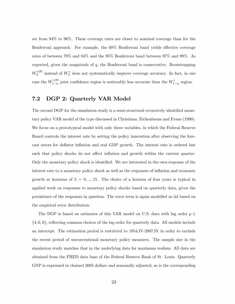
7.2 DGP 2: Quarterly VAR Model

The second DGP for the simulation study is a semi-structural recursively identified mone-

tary policy VAR model of the type discussed in Christiano, Eichenbaum and Evans (1999).

We focus on a prototypical model with only three variables, in which the Federal Reserve

Board controls the interest rate by setting the policy innovation after observing the fore-

cast errors for deflator inflation and real GDP growth. The interest rate is ordered last

such that policy shocks do not affect inflation and growth within the current quarter.

Only the monetary policy shock is identified. We are interested in the own-response of the

interest rate to a monetary policy shock as well as the responses of inflation and economic

growth at horizons of = 0 15. The choice of a horizon of four years is typical in

applied work on responses to monetary policy shocks based on quarterly data, given the

persistence of the responses in question. The error term is again modelled as iid based on

the empirical error distribution.

The DGP is based on estimates of this VAR model on U.S. data with lag order ∈4 6 8, reflecting common choices of the lag order for quarterly data. All models includean intercept. The estimation period is restricted to 1954.IV-2007.IV in order to exclude

the recent period of unconventional monetary policy measures. The sample size in the

simulation study matches that in the underlying data for maximum realism. All data are

obtained from the FRED data base of the Federal Reserve Bank of St. Louis. Quarterly

GNP is expressed in chained 2005 dollars and seasonally adjusted, as is the corresponding

23

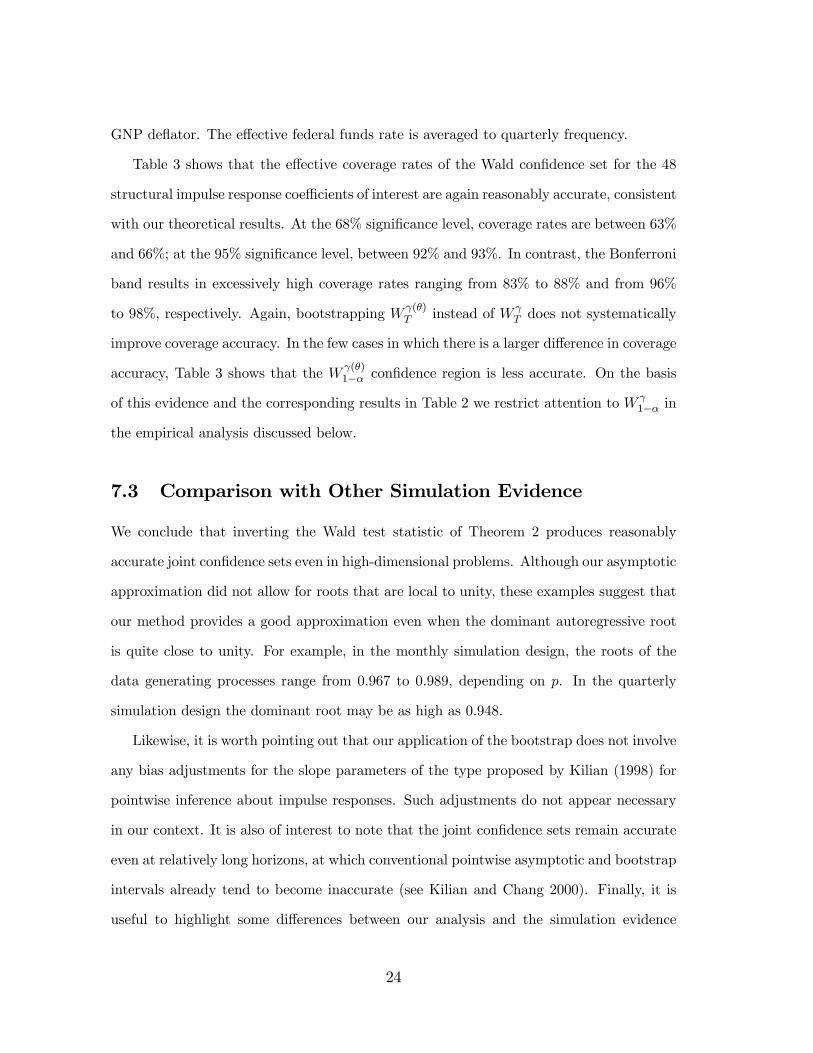
GNP deflator. The effective federal funds rate is averaged to quarterly frequency.

Table 3 shows that the effective coverage rates of the Wald confidence set for the 48

structural impulse response coefficients of interest are again reasonably accurate, consistent

with our theoretical results. At the 68% significance level, coverage rates are between 63%

and 66%; at the 95% significance level, between 92% and 93%. In contrast, the Bonferroni

band results in excessively high coverage rates ranging from 83% to 88% and from 96%

to 98%, respectively. Again, bootstrapping () instead of

does not systematically

improve coverage accuracy. In the few cases in which there is a larger difference in coverage

accuracy, Table 3 shows that the ()1− confidence region is less accurate. On the basis

of this evidence and the corresponding results in Table 2 we restrict attention to 1− in

the empirical analysis discussed below.

7.3 Comparison with Other Simulation Evidence

We conclude that inverting the Wald test statistic of Theorem 2 produces reasonably

accurate joint confidence sets even in high-dimensional problems. Although our asymptotic

approximation did not allow for roots that are local to unity, these examples suggest that

our method provides a good approximation even when the dominant autoregressive root

is quite close to unity. For example, in the monthly simulation design, the roots of the

data generating processes range from 0.967 to 0.989, depending on . In the quarterly

simulation design the dominant root may be as high as 0.948.

Likewise, it is worth pointing out that our application of the bootstrap does not involve

any bias adjustments for the slope parameters of the type proposed by Kilian (1998) for

pointwise inference about impulse responses. Such adjustments do not appear necessary

in our context. It is also of interest to note that the joint confidence sets remain accurate

even at relatively long horizons, at which conventional pointwise asymptotic and bootstrap

intervals already tend to become inaccurate (see Kilian and Chang 2000). Finally, it is

useful to highlight some differences between our analysis and the simulation evidence

24

reported in Lütkepohl et al. (2014). Their simulation design was a bivariate VAR(1)

model with a wide range of different degrees of persistence and sample sizes. The relevant

comparison is to their results for highly persistent VAR processes.

First, whereas Lütkepohl et al. (2014) show that Bonferroni sets are at best mildly

conservative in terms of coverage, we found them to be considerably more conservative for

our simulation designs. One would expect this difference to be largely explained by the

fact that in our simulation designs is much larger than in their study, which puts the

Bonferroni method at a disadvantage.

Second, Lütkepohl et al. (2014) find that the Wald confidence band ()1− has

reasonably accurate coverage for the simulation designs in question when is moderately

large. We show the Wald confidence sets based on 1− and

()1− to be reasonably

accurate for much larger . There is one important difference, however. Because we are

not concerned with the construction of joint confidence bands, we evaluate the coverage

accuracy of the joint Wald confidence sets instead by assessing with what probability the

joint Wald test statistics and

lie outside their respective bootstrap critical region.

Lütkepohl et al. (2014), in contrast, assess the coverage accuracy of the joint confidence

band by recording the relative frequency with which the joint confidence band entirely

includes the corresponding vector of true impulse responses. Hence, the results are not

directly comparable.

Third, because forming two-dimensional confidence bands by the projection method

involves a loss of power, the ()1− confidence band may be wider on average than the

Bonferroni band. Lütkepohl et al. (2014) show by simulation that the Bonferroni bands

indeed in many situations can produce tighter confidence bands than ()1− , while

preserving coverage rates of at least 1−. These situations do not include applications withsomewhat larger , however, as shown in their Table 4. In the latter case,

()1− tends

to have shorter average interval width than the joint Bonferroni band, while maintaining

coverage accuracy.

25

An interesting extension of Lütkepohl et al.’s work would be to compare the finite-

sample coverage accuracy and average width of the confidence bands based on 1− to

bands based on ()1− . We do not pursue this question because our analysis focuses

on joint confidence regions rather than bands. The reason is that the construction of joint

confidence bands based on the Wald confidence region, while facilitating comparisons with

the Bonferroni bands, negates some of the advantages of working with shotgun plots of

the impulse responses based on the joint Wald confidence set. This point is illustrated in

the next section. For expository purposes we focus on the shotgun plots associated with

the 1− confidence region.

8 Empirical Examples

8.1 A VAR Model of U.S. Monetary Policy

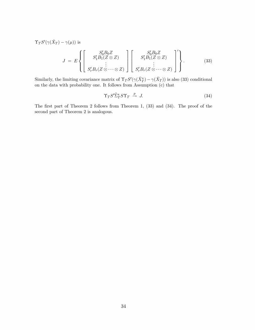
The first example is a VAR(4) model of U.S. monetary policy estimated on quarterly data

for 1954.IV-2007.IV. The variables include GNP deflator inflation, real GNP growth and

the federal funds rate. The dominant autoregressive root is 095. The model is identified

recursively with the federal funds rate ordered last. We are interested in the responses

of the model variables to an unexpected monetary policy tightening, corresponding to an

unexpected increase in the federal funds rate, so = 46.

Figure 1 shows the three shotgun plots obtained by plotting all sets of structural

impulse responses contained in the 68% joint confidence set based on . An easy way

of assessing whether any of these responses is significantly different from zero is to search

for impulse response functions in the joint confidence set that cross the zero line. For

example, Figure 1 shows that the response function of real GNP growth is significantly

negative at the two-quarter horizon in that none of the responses are zero or positive,

while the response function of inflation is distinguishable from the zero line at the 68%

significance level. Moreover, it can be shown that allowing for the joint uncertainty about

26

the elements of the structural impulse response vector suffices to rule out the well-known

price puzzle. This price puzzle refers to the tendency of the price level in VAR models to

exhibit a statistically significant increase in response to an unexpected monetary tightening

based on pointwise confidence intervals.

Exactly the same results would be obtained by constructing the joint confidence band

connecting the uppermost realizations of the shotgun plot at each horizon to form the

upper confidence band and by connecting the lowest realizations by horizon to form the

lower band. In this sense, these two approaches convey the same information. Such a joint

confidence band, however, would tend to obscure information about the shape of a given

response function.

Consider, for example, the response of the level of U.S. real GNP to an unexpected

monetary policy tightening, which is obtained by cumulating the responses of the growth

rate. Standard business cycle theory implies that the increase in real GDP caused by a

unexpected loosening of monetary policy should be hump-shaped. Figure 2 shows this

response obtained by flipping the sign of the cumulated growth rate response shown in

Figure 1. We also added a visual representation of the joint confidence band obtained

by constructing an envelope around the shotgun plot. It is unclear from inspecting the

confidence band, what the shape of the response function is. Indeed, the confidence band

is wide enough to accommodate any number of shapes of the response function, some

consistent with economic theory and some not.

Most economists would be interested in the question of whether economic models im-

plying a hump-shaped response of real output to a monetary policy shock are consistent

with the evidence in Figure 2. If one is willing to define a hump shape, as most macroecono-

mists are prone to, based on our reading of the VAR literature, one can run an iterative

search on the response functions contained in the 68% joint confidence set to determine

whether any of the response functions in the set are inconsistent with this hump shape.

Evidence that all response functions in the 68% confidence set are hump-shaped would

27

lead us to reject the hypothesis that there is no hump in the response function. Evidence

that none of the response functions in the set is hump-shaped, in contrast, would imply

a rejection of the hypothesis of a hump-shaped response. Evidence that some response

functions in the set are hump-shaped and some are not, would be imply that neither

hypothesis can be rejected at the 68% confidence level.

For example, for expository purposes, we may define a hump-shaped response function

for U.S. real GNP as one whose maximum occurs between horizons 1 and 15. Given that

the response starts at zero by construction, effectively this definition rules out response

functions that reach their maximum at horizon 15. Table 4 shows that about 31% of

the response functions in Figure 2 are not hump-shaped by this minimal definition of a

hump shape, so we cannot be confident at the 68% level that the response function of

U.S. real GNP is hump-shaped. The data in the shotgun plot are consistent with other

interpretations of the shape of the response function. Similar results also hold at the 95%

significance level. This is more information than could have been gleaned from the joint

confidence band. In this particular example, one could have inferred that there must be

at least one response function that is not hump-shaped from the fact that upper bound of

the confidence band peaks at horizon 15. On the other hand, one could not have inferred

the presence of hump-shaped response functions from the joint confidence band.

Our results are qualitatively robust to further strengthening the definition of a hump-

shaped response function for U.S. real GNP by imposing the additional requirement of

piecewise monotonicity such that the slope of the impulse response function is positive to

the left of the peak response and negative to the right of the peak response. This reduces

the percentage of models in the 68% confidence set that generate hump-shaped responses

to about 16%, as shown in Table 4. Similar results hold at the 95% confidence level.

28

8.2 A VAR Model of the Stagflationary Effects of Oil Price

Shocks

Our second empirical example focuses on a hypothesis that involves multiple response

functions. Evidence that the economy remains below potential, while inflation continues

to rise, is inconsistent with the standard accelerationist model of the macroeconomy and

thus would seem to require a different explanation, presumably one based on domestic

supply shocks that shift the Phillips curve. A popular argument in macroeconomics has

been that oil price shocks in particular may act as such supply shocks for the U.S. economy.

Thus, the question of whether oil price shocks are stagflationary has a long tradition in

macroeconomics (see, e.g., Blanchard 2002; Barsky and Kilian 2004; Kilian 2008).

We address this question by postulating a VAR(4) model for the U.S. economy for

the percent change in the real WTI price of crude oil, GDP deflator inflation and real

GDP. The data are quarterly and the estimation period is 1987.I-2013.II. The starting

date was chosen for illustrative purposes, given evidence for a possible structural break in

the relationship between the real price of oil and U.S. real GDP in 1987. The dominant

autoregressive root is 085. The model is identified recursively with the real price of oil

ordered first. We focus on the effect of an unanticipated increase in the real price of oil

on the real price of oil, on the change in inflation and on U.S. real GDP growth.

Figure 3 shows that the shotgun plots for the change in inflation and for real GDP

growth cover the zero line at all horizons. This fact alone, however, tells us nothing about

the question of whether these responses are stagflationary. To answer the latter question

we need to look at these two response functions pairwise for each model in the joint

confidence set and verify whether the responses of ∆+ and ∆+, where stands for

GDP deflator inflation and ∆ for real GDP growth, to an oil price shock are of opposite

sign for all horizons of interest (see, e.g., Kilian 2008). It is immediately obvious that this

type of information cannot be inferred from joint confidence bands, but may be computed

based on the shot-gun plot. The first row in Table 5 shows that, at the 68% significance

29

level and looking jointly at horizons = 1 15 not a single structural model estimate

in the joint confidence set is consistent with the hypothesis of stagflationary responses to

oil price shocks. Thus, we can rule out that hypothesis. One might have conjectured that

increasing the confidence level would lead us to revise this statement, but the first row in

Table 5 shows that the same result holds at the 95% significance level.

It would have been tempting to conclude based on a joint confidence band that Figure

3 allows for stagflationary responses at horizon = 1 15 because both bands include

positive as well as negative values, so hypothetically a stagflationary response would fit

within this confidence band for = 1 15. This conclusion, however, would have been

wrong, considering the evidence in the first row of Table 5. This example reinforces our

point that joint confidence bands may obscure important information about the shapes of

impulse response functions.

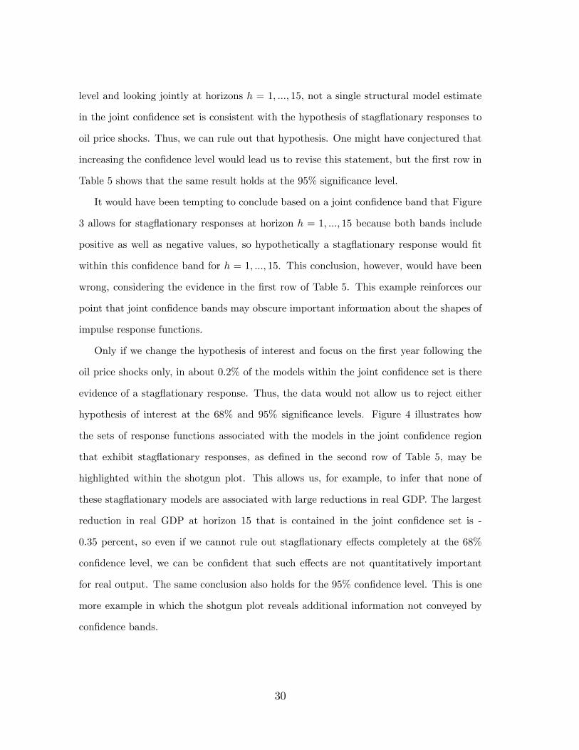
Only if we change the hypothesis of interest and focus on the first year following the

oil price shocks only, in about 0.2% of the models within the joint confidence set is there

evidence of a stagflationary response. Thus, the data would not allow us to reject either

hypothesis of interest at the 68% and 95% significance levels. Figure 4 illustrates how

the sets of response functions associated with the models in the joint confidence region

that exhibit stagflationary responses, as defined in the second row of Table 5, may be

highlighted within the shotgun plot. This allows us, for example, to infer that none of

these stagflationary models are associated with large reductions in real GDP. The largest

reduction in real GDP at horizon 15 that is contained in the joint confidence set is -

0.35 percent, so even if we cannot rule out stagflationary effects completely at the 68%

confidence level, we can be confident that such effects are not quantitatively important

for real output. The same conclusion also holds for the 95% confidence level. This is one

more example in which the shotgun plot reveals additional information not conveyed by

confidence bands.

30

9 Conclusion

We considered the problem of constructing joint confidence sets for subsets of structural

impulse responses that remain asymptotically valid even when the joint limiting distri-

bution of the structural impulse response estimators becomes degenerate, which occurs

when the number of responses considered exceeds the number of model parameters. We

made the case that applied users should invert the joint Wald test statistic to obtain such

a joint confidence set. We considered two alternative specifications of the Wald test sta-

tistic. Both are asymptotically valid and were shown to imply joint confidence sets with

reasonably accurate coverage in finite samples. Our simulation evidence suggested that in

the few cases, in which there is a noticeable difference in coverage accuracy, our preferred

specification is more accurate in finite samples.

We proposed to represent the sets of structural responses associated with the estimates

in the joint confidence set in the form of shotgun plots of the impulse response functions.

We made the case that this approach preserves additional information about the shape

of the impulse response functions that is lost when the results are presented in the form

of joint confidence bands. In fact, the use of shotgun plots is essential for answering

many of the key questions applied users want to answer based on structural VAR models.

These questions relate not so much to whether a particular set of responses is significantly

different from zero, although that question as well can be answered with the help of shotgun

plots, but whether multiple sets of response functions follow the shape and pattern implied

by economic theory. We demonstrated by example that the latter type of question cannot

be answered based on joint confidence bands, whether constructed from Bonferroni bounds

or by applying the projection method to Wald confidence sets. Appropriate answers can be

obtained and visualized, however, on the basis of the information contained in the shotgun

plots of the impulse response functions. Assessing the validity of restrictions on sets of

structural impulse responses requires knowledge of which of the simulated realizations

of the structural impulse responses were generated by the same structural model. This

31

information is not preserved by more conventional methods of joint inference.

Our theoretical analysis involved a novel approach to approximating the distribution

of test statistics with an asymptotically singular covariance matrix that is distinct from

alternative approaches such as Andrews (1987) and is of independent interest for other

applications. Although we focused on the construction of joint confidence sets about struc-

tural impulse responses, our results on bootstrapping Wald statistics for impulse response

vectors with a degenerate joint asymptotic distribution can also be applied in a variety

of other contexts. For example, they facilitate the design of statistical tests about vari-

ous features of structural impulse response functions (e.g., Lütkepohl 1996). They also are

relevant for the development of impulse response matching estimators of the structural pa-

rameters of dynamic stochastic general equilibrium models (see Guerron-Quintana, Inoue

and Kilian 2014). A third example, in which our bootstrap approach can help overcome

rank deficiencies in the covariance matrix, is tests for multi-step noncausality (see Lütke-

pohl and Burda 1997).

In this paper, we followed much of the VAR literature on impulse response analysis by

focusing on Wald test statistics. An obvious extension would be to apply our approach to

the LR test statistic. We defer this extension to future research, given the high coverage

accuracy of the Wald confidence region in our simulation study. Another interesting

question for future research will be how to construct optimal joint confidence regions for

structural impulse responses.

32

10 Technical Appendix

Proof of Theorem 1.

It follows from the Schur decomposition theorem (Theorem 13 of Magnus and Neudecker,

1999, p.16) that there exists an orthonormal matrix whose columns are eigenvectors of

000 and a diagonal matrix Λ whose diagonal elements are the eigenvalues of 0

00 such

that

0000 = Λ (29)

Stack the eigenvectors associated with the largest eigenvalues of 000 in 0 and let

0 = . Using a subset of the − 0 remaining eigenvectors that are not used in 0, form

1 such that 011 contains no row vector of zeros. Let 1 denote the number of columns

in 1. Using a subset of the −0− · · ·−−1 remaining eigenvectors, that are not used in0, 1,...−1, form so that

0 contains no row vector of zeros. Let be the number

of columns in . Stop when 0 + 1 + · · · + = . With some abuse of notation, let

= [1 2 · · · ]. Then it follows from the definition of and Assumption (b) that

Υ0(( )− ()) = 00 + −

1201( ⊗ ) + (

− 12 )

=

⎡⎢⎢⎣000

011( ⊗ )...

0( ⊗ · · ·⊗ )

⎤⎥⎥⎦+ (1) (30)

It furthermore follows from (30) and Assumption (a) that

Υ0(( )− ())

→

⎡⎢⎢⎣000

011( ⊗ )...

0( ⊗ · · ·⊗ )

⎤⎥⎥⎦ (31)

Because of Assumptions (a) and (b) and because of the continuity of eigenvalues and

eigenvectors as a function of matrices, we also know that

Υ0((∗

)− ( ))→

⎡⎢⎢⎣000

∗011(

∗ ⊗ ∗)...

0(∗ ⊗ · · ·⊗ ∗)

⎤⎥⎥⎦ (32)

where the convergence is with respect to the bootstrap probability measure conditional

on the data with probability one, Therefore Theorem 1 follows from (31) and (32).

Proof of Theorem 2. It follows from (32) that the limiting covariance matrix of

33

Υ0(( )− ()) is

=

⎧⎪⎪⎨⎪⎪⎩⎡⎢⎢⎣

000011( ⊗ )

...0( ⊗ · · ·⊗ )

⎤⎥⎥⎦⎡⎢⎢⎣

000011( ⊗ )

...0( ⊗ · · ·⊗ )

⎤⎥⎥⎦0⎫⎪⎪⎬⎪⎪⎭ (33)

Similarly, the limiting covariance matrix of Υ0((∗

)− ( )) is also (33) conditional

on the data with probability one. It follows from Assumption (c) that

Υ0bΣ∗Υ

→ (34)

The first part of Theorem 2 follows from Theorem 1, (33) and (34). The proof of the

second part of Theorem 2 is analogous.

34

11 References

1. Andrews, D.W.K., (1987), “Asymptotic Results for Generalized Wald Tests,” Econo-

metric Theory, 3, 348-358.

2. Antoine, B., and E. Renault (2012), “Efficient Minimum Distance Estimation with

Multiple Rates of Convergence,” Journal of Econometrics, 1709, 350-367.

3. Bao, Y., and A. Ullah, (2007), “The Second-Order Bias and Mean Squared Error of

Estimators in Time Series Models,” Journal of Econometrics, 140, 650-669.

4. Bao, Y. (2007), “ The Approximate Moments of the Least Squares Estimator for the

Stationary Autoregressive Model Under a General Error Distribution,” Econometric

Theory, 23, 1013-1021.

5. Barsky, R.B., and L. Kilian (2004), “Oil and the Macroeconomy since the 1970s,”

Journal of Economic Perspectives, 18, Fall, 115-134.

6. Benkwitz, A., Lütkepohl, H., and M.H. Neumann (2000), “Problem Related to Boot-

strapping Impulse Responses of Autoregressive Processes,” Econometric Reviews, 19,

69-103.

7. Berkowitz, J., and L. Kilian (2000), “Recent Developments in Bootstrapping Time

Series,” Econometric Reviews, 19, 1-54.

8. Blanchard, O.J. (1989), “A Traditional Interpretation of Macroeconomic Fluctua-

tions,” American Economic Review, 79, 1146-1164.

9. Blanchard, O.J. (2002), “Comments on ‘Do We Really Know that Oil Caused the

Great Stagflation? A Monetary Alternative’ by Robert Barsky and Lutz Kilian,” in:

Bernanke, B.S., and K. Rogoff (eds.), NBER Macroeconomics Annual, Cambridge,

MA: MIT Press, 183-192.

10. Brüggemann, R., C. Jentsch, and C. Trenkler (2014), “Inference in VARs with Con-

ditional Heteroskedasticity of Unknown Form,” mimeo, University of Mannheim.

11. Cochrane, J.H. (1994), “Shocks,” Carnegie-Rochester Conference Series on Public

Policy, 41, 295-364.

12. Christiano, L., M. Eichenbaum and C. Evans (1999), “Monetary policy shocks: what

have we learned and to what end?”, in J.B Taylor and M. Woodford (eds.), Handbook

of Macroeconomics, 1, Amsterdam: Elsevier/North Holland, 65-148.

13. Freedman, D., (1984), “On Bootstrapping Two-Stage Least-Squares Estimators in

Stationary Linear Models,” Annals of Statistics, 12, 827-842.

14. Guerron-Quintana, P., Inoue, A., and L. Kilian (2014), “Impulse Response Matching

Estimators for DSGE Models,” mimeo, University of Michigan.

15. Hall, P. (1992), The Bootstrap and Edgeworth Expansion, Springer: New York.

16. Inoue, A., and L. Kilian (2013), “Inference on Impulse Response Functions in Struc-

tural VAR Models,” Journal of Econometrics, 177, 1-13.

17. Jordà, Ò. (2009), “Simultaneous Confidence Regions for Impulse Responses,” Review

of Economics and Statistics, 91, 629-647.

35

18. Kilian, L. (1998), “Small-Sample Confidence Intervals for Impulse Response Func-

tions,” Review of Economics and Statistics, 80, 218-230.

19. Kilian, L. (1999), “Finite-Sample Properties of Percentile and Percentile- Bootstrap

Confidence Intervals for Impulse Responses,” Review of Economics and Statistics,

81, 652-660.

20. Kilian, L. (2001), “Impulse Response Analysis in Vector Autoregressions with Un-

known Lag Order”, Journal of Forecasting, 20, 161-179.

21. Kilian, L. (2008), “A Comparison of the Effects of Exogenous Oil Supply Shocks

on Output and Inflation in the G7 Countries”, Journal of the European Economic

Association, 6, 78-121.

22. Kilian, L. (2013), “Structural Vector Autoregressions,” in: Handbook of Research

Methods and Applications in Empirical Macroeconomics, N. Hashimzade and M.

Thornton (eds.), Cheltenham, UK: Edward Elgar, 515-554.

23. Kilian, L., and P.-L. Chang (2000), “How Accurate are Confidence Intervals for

Impulse Responses in Large VAR Models?”, Economics Letters, 69, 299-307.

24. Kilian, L., and Y.J. Kim (2011), “How Reliable Are Local Projection Estimators of

Impulse Responses?” Review of Economics and Statistics, 93, 1460-1466.

25. Lütkepohl, H. (1990), “Asymptotic Distributions of Impulse Response Functions and

Forecast Error Variance Decompositions of Vector Autoregressive Models,” Review

of Economics and Statistics, 72, 116-25.

26. Lütkepohl, H. (1996), “Testing for Nonzero Impulse Responses in Vector Autoregres-

sive Processes,” Journal of Statistical Planning and Inference, 50, 1-20.

27. Lütkepohl, H., Staszewska-Bystrova, A., and P. Winker (2013), “Comparison of

Methods for Constructing Joint Confidence Bands for Impulse Response Functions,”

forthcoming: International Journal of Forecasting.

28. Lütkepohl, H., Staszewska-Bystrova, A., and P. Winker (2014), “Confidence Bands

for Impulse Responses: Bonferroni versus Wald,” manuscript, DIW Berlin.

29. Lütkepohl, H., and M.M. Burda (1997), “Modified Wald Tests under Nonregular

Conditions,” Journal of Econometrics, 78, 315-332.

30. Lütkepohl, H., and D.S. Poskitt (1991), “Estimating Orthogonal Impulse Responses

via Vector Autoregressive Models,” Econometric Theory, 7, 487-496.

31. Magnus, J.R., and H. Neudecker (1999), Matrix Differential Calculus with Applica-

tions in Statistics and Econometrics, Revised Edition, Wiley: Chichester: England.

32. Phillips, P.C.B. (1989), “Partially Identified Econometric Models,” Econometric The-

ory, 5, 181-240.

33. Sims, C.A., J.H. Stock and M.W. Watson (1990), “Inference in Linear Time Series

Models with Some Unit Roots,” Econometrica, 58, 113-144.

34. Sims, C.A., and T. Zha, (1999), “Error Bands for Impulse Responses,” Econometrica,

67, 1113-1156.

35. Woodford, M. (2003), Interest and Prices: Foundations of a Theory of Monetary

Policy. Princeton: Princeton University Press.

36

Table 1: Relative Volumes of Bonferroni and Wald Confidence Regions

Confidence level 1 0.9 M

1B ,

1bandW 1W

2 1.01 1.22 0.95 3 1.02 1.65 0.87 4 1.03 2.46 0.76 5 1.03 3.94 0.65 6 1.04 6.67 0.54 7 1.05 11.89 0.44 8 1.05 22.17 0.35 9 1.06 43.02 0.28 10 1.07 86.54 0.22

NOTES: The volume of the 1 confidence region refers to an M -dimensional cube, where M is the length of the vector . All results are normalized relative to the volume of the joint confidence region associated with the precise confidence box that represents the tightest two-dimensional confidence box possible. 1B

refers to the joint confidence region implied by

Bonferroni confidence band. ,1

bandW refers to the joint confidence region implied by the

confidence band proposed in Lütkepohl et al. (2014), and 1W relates to the joint confidence

region implied by the Wald test statistic.

Table 2: Joint inference for all impulse responses at horizon 0,...,17h in a monthly oil market VAR model

Coverage Rates (%)

1W ( )

1W 1B

Nominal 68 95 68 95 68 95 6p 70.8 93.8 63.0 93.8 84.0 97.0

12p 65.6 96.0 65.4 94.0 80.6 98.0

24p 67.2 94.2 71.6 95.4 78.8 98.0

NOTES: Coverage rates based on 500 trials, each of which involves 1,0001,000 bootstrap replications. The model is motivated by the analysis in Kilian (2009). Based on the oil market data set in Kilian (2009), alternative DGPs are constructed for lag orders 6,12, 24 .p 1W

and ( )1W stand for the two alternative joint Wald confidence regions discussed in section 6 and

1B for the Bonferroni set.

Table 3: Joint inference for all responses to the monetary policy shock at horizon 0,...,15h in a quarterly monetary policy VAR model

Coverage Rates (%)

1W ( )

1W 1B

Nominal 68 95 68 95 68 95 4p 63.4 93.2 61.0 92.0 87.6 98.2

6p 66.4 93.4 64.2 93.0 87.6 98.0

8p 66.4 92.2 62.6 89.2 83.2 96.4

NOTES: Coverage rates based on 500 trials, each of which involves 1,0001,000 bootstrap replications. The DGP is a prototypical recursively identified monetary policy VAR model for U.S. deflator inflation, real GDP growth and the federal funds rate, as discussed in Kilian (2013). Based on data for 1954.III-2007.IV, alternative DGPs are constructed from the fitted models for lag orders 4, 6,8 .p 1W

and ( )1W stand for the two alternative joint Wald confidence

regions discussed in section 6 and 1B for the Bonferroni set.

Table 4: Percentage of models in joint Wald confidence set consistent with a hump-shaped

response function of real GNP to an unexpected loosening of monetary policy

NOTES: Based on the model underlying Figure 2 and a minimal definition of a hump shaped response as a response reaching its maximum between horizon 1 and 15. The optional piecewise monotonicity constraint restricts the slope of the impulse response function to be positive to the left of the peak response and negative to the right of the peak response.

Table 5: Percentage of models in joint Wald confidence set inconsistent with a stagflationary response to an unexpected increase in the real price of oil

Joint Confidence Level Horizons ( h ) 68% 95%

1,…,15 100.0% 100.0% 1,…,4 99.8% 99.8%

NOTES: Based on the model underlying Figure 3. The stagflation hypothesis translates to the

responses of t h and t hy to the oil price shock being of opposite sign for all horizons h of

interest and the inflation acceleration being positive at horizon 1.

Joint Confidence Level 68% 95%

No piecewise monotonicity imposed 69.0% 70.1% Piecewise monotonicity imposed 15.6% 15.3%

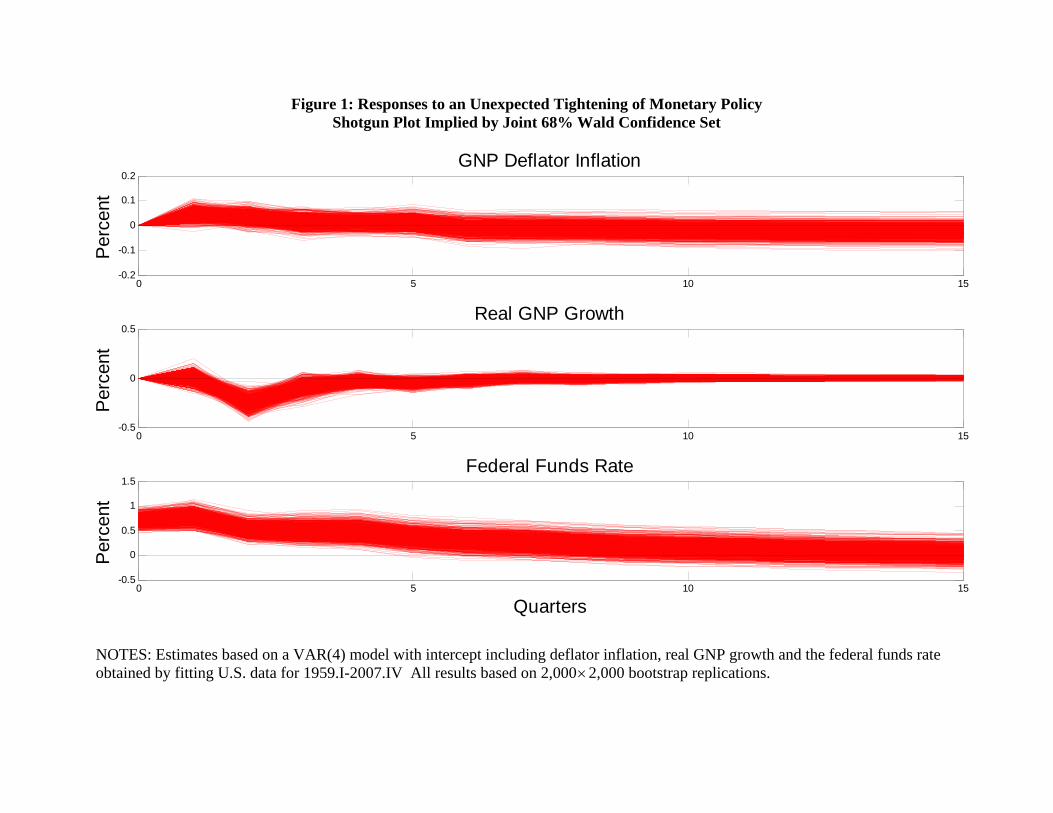
0 5 10 15-0.2

-0.1

0

0.1

0.2GNP Deflator Inflation

Perc

ent

0 5 10 15-0.5

0

0.5Real GNP Growth

Per

cent

0 5 10 15-0.5

0

0.5

1

1.5Federal Funds Rate

Quarters

Perc

ent

Figure 1: Responses to an Unexpected Tightening of Monetary Policy Shotgun Plot Implied by Joint 68% Wald Confidence Set

NOTES: Estimates based on a VAR(4) model with intercept including deflator inflation, real GNP growth and the federal funds rate obtained by fitting U.S. data for 1959.I-2007.IV All results based on 2,0002,000 bootstrap replications.

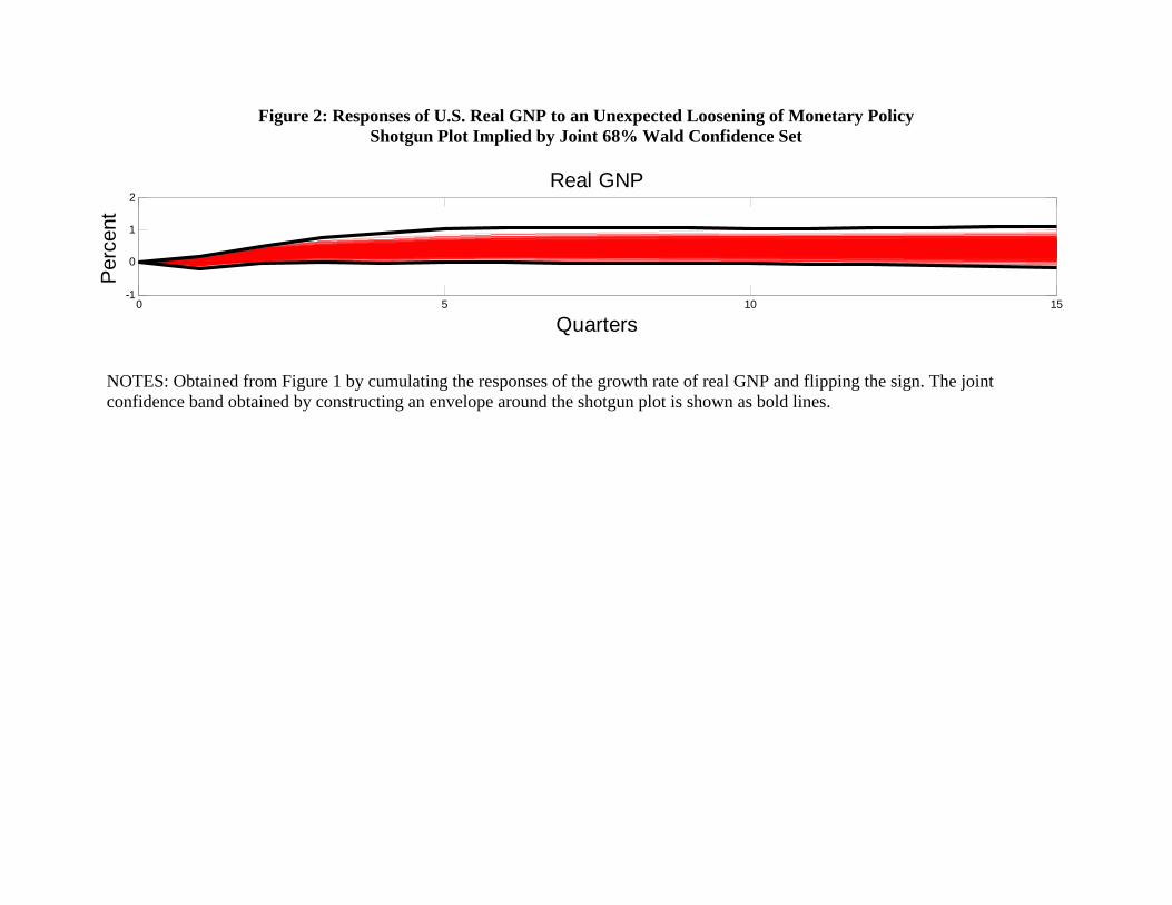
0 5 10 15-1

0

1

2Real GNP

Perc

ent

Quarters

Figure 2: Responses of U.S. Real GNP to an Unexpected Loosening of Monetary Policy Shotgun Plot Implied by Joint 68% Wald Confidence Set

NOTES: Obtained from Figure 1 by cumulating the responses of the growth rate of real GNP and flipping the sign. The joint confidence band obtained by constructing an envelope around the shotgun plot is shown as bold lines.

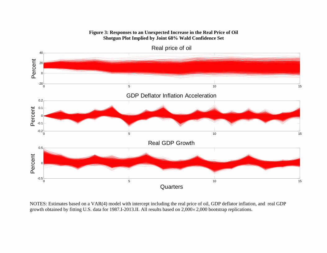
0 5 10 15-20

0

20

40Real price of oil

Perc

ent

0 5 10 15-0.2

-0.1

0

0.1

0.2GDP Deflator Inflation Acceleration

Per

cent

0 5 10 15-0.5

0

0.5Real GDP Growth

Quarters

Perc

ent

Figure 3: Responses to an Unexpected Increase in the Real Price of Oil Shotgun Plot Implied by Joint 68% Wald Confidence Set

NOTES: Estimates based on a VAR(4) model with intercept including the real price of oil, GDP deflator inflation, and real GDP growth obtained by fitting U.S. data for 1987.I-2013.II. All results based on 2,0002,000 bootstrap replications.

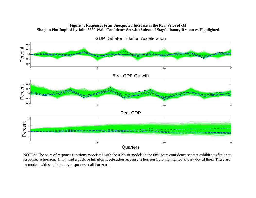
0 5 10 15

-0.2

-0.1

0

0.1

0.2

GDP Deflator Inflation Acceleration

Perc

ent

0 5 10 15-0.4

-0.2

0

0.2

0.4

Real GDP Growth

Per

cent

0 5 10 15

-1

0

1

2

Real GDP

Quarters

Perc

ent

Figure 4: Responses to an Unexpected Increase in the Real Price of Oil Shotgun Plot Implied by Joint 68% Wald Confidence Set with Subset of Stagflationary Responses Highlighted

NOTES: The pairs of response functions associated with the 0.2% of models in the 68% joint confidence set that exhibit stagflationary responses at horizons 1,..., 4 and a positive inflation acceleration response at horizon 1 are highlighted as dark dotted lines. There are no models with stagflationary responses at all horizons.