Standard Title Page - Virginia Tech

Standard Title Page - Report on State Project Report No.

Report Date

No. Pages

Type Report: Final

Project No.: 73977

VTRC 06-CR13 June 2006 76 Period Covered: January 2002 – May 2006

Contract No.

Title: Stability of Column-Supported Embankments

Key Words: Column-supported embankment, numerical analysis, reliability analysis, deep mixing.

Authors: George M. Filz and Michael P. Navin

Performing Organization Name and Address: Virginia Transportation Research Council 530 Edgemont Road Charlottesville, VA 22903

Sponsoring Agencies’ Name and Address Virginia Department of Transportation 1401 E. Broad Street Richmond, VA 23219

Supplementary Notes

Abstract

Column-supported embankments have a great potential for application in the coastal regions of Virginia, where highway embankments are often constructed on soft ground. The columns can be driven piles, vibro-concrete columns, deep-mixing-method columns, stone columns, or other suitable types. Column-supported embankments are used to accelerate construction by eliminating consolidation times that are needed for preloading and surcharging operations associated with conventional prefabricated vertical drains.

This study has resulted in a development of new numerical stress-strain analyses to evaluate the stability of

embankments supported on columns installed by deep mixing method. Such analyses reflect the multiple realistic failure mechanisms that can occur when strong columns are installed in weak soil. Detailed recommendations for performing numerical analyses are presented. The findings are also expected to apply to vibro-concrete columns, because they, like deep-mixing-method columns, are strong in compression but weak in bending and tension.

The study also recommends the use of reliability analyses in conjunction with the stability analysis. Reliability

analyses are necessary, because deep-mixed materials can be highly variable and because typical variations in the strength of the surrounding clay can induce abrupt tensile failure in columns. Additional benefit of the reliability-based design is that it permits rational development of statistically-based specifications for constructing deep-mixed materials.

FINAL CONTRACT REPORT

STABILITY OF COLUMN-SUPPORTED EMBANKMENTS

George M. Filz Professor

Michael P. Navin

Post-doctoral Research Associate

Via Department of Civil and Environmental Engineering Virginia Polytechnic Institute & State University

Project Manager Edward J. Hoppe, Ph.D., P.E., Virginia Transportation Research Council

Contract Research Sponsored by Virginia Transportation Research Council

(Virginia Transportation Research Council (A partnership of the Virginia Department of Transportation

and the University of Virginia since 1948)

Charlottesville, Virginia

June 2006 VTRC 06-CR13

borrego

Typewritten Text

Copyright by the Virginia Center for Transportation Innovation and Research. George M. Filz and Michael P. Navin. “Stability of Column-Supported Embankments,” Virginia Transportation Research Council 530 Edgemont Road Charlottesville, VA 22903, Report No. VTRC 06-CR13, June 2006.

ii

NOTICE

The project that is the subject of this report was done under contract for the Virginia Department of Transportation, Virginia Transportation Research Council. The contents of this report reflect the views of the authors, who are responsible for the facts and the accuracy of the data presented herein. The contents do not necessarily reflect the official views or policies of the Virginia Department of Transportation, the Commonwealth Transportation Board, or the Federal Highway Administration. This report does not constitute a standard, specification, or regulation. Each contract report is peer reviewed and accepted for publication by Research Council staff with expertise in related technical areas. Final editing and proofreading of the report are performed by the contractor.

Copyright 2006 by the Commonwealth of Virginia.

iii

ABSTRACT Column-supported embankments have great potential for application in coastal regions in

Virginia where embankments for transportation applications are often constructed on soft ground. The columns can be driven piles, vibro-concrete columns, deep-mixing-method columns, stone columns, or other types of suitable columns. Column-supported embankments can be used to accelerate construction by eliminating the consolidation times that are needed for preloading and surcharging with prefabricated vertical drains. Column-supported embankments can also be used to protect existing adjacent facilities against induced settlement, such as protecting an existing pavement when an embankment is being widened.

Established procedures are available for analyzing the stability of embankments

supported on driven piles and on stone columns. Summaries of these procedures are presented in appendices to this report. For embankments supported on deep-mixing-method columns, limit equilibrium methods of slope stability analysis are often used, but these methods only reflect composite shearing through the columns and soil, and they do not directly reflect the more critical failure modes of column bending and tilting that can occur when the columns are strong.

A principle outcome of this research is to recommend that VDOT engineers and their

consultants use numerical stress-strain analyses to evaluate the stability of embankments supported on columns installed by the deep mixing method. Such analyses do reflect the multiple realistic failure mechanisms that can occur when strong columns are installed in weak ground. Detailed recommendations for performing numerical analyses are presented.

Another important recommendation is that VDOT engineers and their consultants use

reliability analyses in conjunction with numerical analyses of the stability of embankments supported on deep-mixing-method columns. Reliability analyses are necessary because deep-mixed materials can be highly variable and because typical variations in the strength of the surrounding clay can induce abrupt tensile failure in the columns, unless properly accounted for in reliability-based design. As part of this research, a spreadsheet that facilitates reliability analyses has been provided to VTRC.

An additional benefit of reliability-based design is that it permits rational development of

statistically based specifications for constructing deep-mixed materials. Such specifications can reduce construction contract administration problems because they allow for some low strength values while still providing assurance that the overall design intent is being met.

Although this research focused on columns installed by the deep mixing method, the

findings are also expected to apply to vibro-concrete columns because they, like deep-mixing-method columns, are strong in compression but have low bending and tensile strength.

1

FINAL CONTRACT REPORT

STABILITY OF COLUMN-SUPPORTED EMBANKMENTS

George M. Filz Professor

Michael P. Navin

Post-doctoral Research Associate

Via Department of Civil and Environmental Engineering Virginia Polytechnic Institute & State University

INTRODUCTION A research project sponsored by Virginia Transportation Research Council and titled

“Columnar Reinforcement of Soft Ground beneath Roadway Embankments” has generated two VTRC reports. This report addresses stability of column-supported embankments. A companion report addresses design of bridging layers in column-supported embankments.

Column-supported embankments are constructed over soft ground to accelerate

construction, improve embankment stability, control total and differential settlements, and protect adjacent facilities. The columns that extend into and through the soft ground can be of several different types: driven piles, vibro-concrete columns, deep-mixing-method columns, stone columns, etc. The columns are selected to be stiffer and stronger than the existing site soil, and if properly designed, they can prevent excessive movement of the embankment.

Column-supported embankments are in widespread use in Japan, Scandinavia, and the

United Kingdom, and they are becoming more common in the U.S. and other countries. The column-supported embankment technology has potential application at many soft-ground sites, including coastal areas where new embankments are being constructed and existing embankments are being widened.

An alternative to column-supported embankments is use of prefabricated vertical drains

combined with gradual placement of the embankment fill. This well-established technique can permit construction of embankments on soft ground at a lower construction cost than by using the column-supported embankment technology. However, use of vertical drains and gradual embankment placement requires considerable time for gradual consolidation and strengthening of the soft ground, and this approach can also induce settlement in adjacent facilities, such as would occur when an existing road embankment is being widened. If accelerated construction is necessary, or if adjacent existing facilities need to be protected, then column-supported embankments may be an appropriate technical solution.

2

The cost of column-supported embankments depends on several design features, including the type, length, diameter, spacing, and arrangement of columns. Geotechnical design engineers establish these details based on considerations of load transfer, settlement, and stability. A separate VTRC report by Filz and Smith (2006) addresses the load transfer and settlement issues. This report addresses stability. The primary emphasis in the main body of this report is on stability of embankments supported on columns installed by the deep mixing method because (1) new embankments at the I-95/U.S. Route 1 interchange, in Alexandria, Virginia, were being designed using columns installed by the deep mixing method at the time this research project was initiated and (2) more uncertainty exists in the literature about this case than for embankments supported on driven piles or stone columns.

In the deep mixing method, stabilizers are mixed into the ground using rotary mixing

tools to increase the strength and decrease the compressibility of the ground. In the dry method of deep mixing, dry lime, cement, fly ash, or other stabilizers are delivered pneumatically to the mixing tool at depth. In the wet method of deep mixing, cement-water slurry is introduced through the hollow stem of the mixing tools.

Although the focus of this report is on deep-mixing-method columns, many of the

techniques described here can also be used for vibro-concrete columns because they also have high compressive strength and low bending and tensile strength. In addition, stability analysis methods for embankments supported on piles and stone columns are presented in Appendices A and B, respectively. Consequently, this report can be used as a reference for stability of embankments supported on a wide variety of column types.

This research is part of a larger project that has spanned several years of involvement by

the authors. All the details of the research cannot be covered in this summary report, which instead describes the key findings and the procedures that would be used by design engineers in practice. Additional information is available in the dissertation by Navin (2005).

PURPOSE AND SCOPE The primary purpose of this research is to develop reliable procedures that geotechnical

engineers can use to analyze the stability of column-supported embankments. Existing procedures are available for analysis of the stability of embankments supported on piles and stone columns, and these are presented in the appendices. Reliability-based approaches were developed for stability analysis of embankments supported on columns installed by the deep mixing method. Deep-mixed materials are variable, and this has an important impact on the procedures that should be used to produce reliable designs. The stability analysis methods presented here for embankments on deep-mixing-method columns are expected to also apply to vibro-concrete columns.

The scope of this research includes: • A review of the pertinent literature on stability of column-supported embankments.

3

• Compilation and statistical analyses of data sets of strength and stiffness of deep-mixed materials.

• Limit equilibrium analyses and numerical stress-strain analyses of field cases

histories and centrifugal model studies. • Reliability analyses of slope stability for embankments supported on deep-mixed

materials. • Development of recommendations for stability analysis of column-supported

embankments. The scope of this report does not include design of bridging layers for column-supported

embankments. Bridging layer design is covered in a report by Filz and Smith (2006).

METHODS This section describes the methods and procedures that were used for the literature

review, data collection and statistical analyses for deep-mixed material strength and stiffness, numerical stress-strain and limit equilibrium analyses, reliability analyses, and development of analysis and design procedures.

Methods for the Literature Review

The literature review was based on searches using Compendex®, Web of Science®, and

other search engines, including those supported by the American Society of Civil Engineers, the Federal Highway Administration, and the Swedish Geotechnical Institute. The contents of relevant journals and conference proceedings were also surveyed. Altogether, about 500 literature sources were reviewed. A comprehensive bibliography is available upon request.

Methods for Data Collection and Statistical Analyses

of Deep-Mixed Material Strength and Stiffness Based on personal contacts, and under the sponsorship of the U.S. National Deep Mixing

Program, unconfined compressive strength data from nine deep mixing construction projects were collected. One of these is VDOT’s interchange re-construction project at the intersection of I-95 and US Route 1 in Alexandria, Virginia. Altogether, these nine projects produced 13 data sets for analyses based on differences in construction technique, subsurface conditions, and sampling technique. In total, 7,079 strength data points were collected.

The strength data were analyzed to produce values of mean, standard deviation, and

coefficient of variation for each data set. Regression analyses were applied to the data to identify controllable parameters that influence strength. After the influence of controllable trends was removed, new values of coefficient of variation were computed to better represent the inherent variability of deep-mixed materials.

4

The strength data were compared to four standard distributions: normal, lognormal, uniform, and triangular. Goodness-of-fit tests were performed using the Chi-squared test and the Kolmogorov-Smirnov test. Both of these tests are described in Ang and Tang (1975).

For three of the data sets, sufficient information was available to evaluate spatial

correlation and compute the autocorrelation distance. The amount of spatial correlation was determined using plots of correlation versus distance. These plots, which are known as correlograms, were determined using a four-step process: (1) column coordinates were used to find the distance from each column to every other column in a data set, (2) pairs of columns were then sorted according to separation distance and stored along with the strength measurements for the columns, (3) a “lag distance” was used to collect pairs of columns into discrete bins according to their separation distance, and (4) the correlation between strength values for pairs of columns was plotted as a function of separation distance. Variowin (Pannatier 1996) is a computer program that was used to perform all four of these steps in two dimensions using the “average value” and “minimum value” methods recommended in the Variowin manual. The autocorrelation distance was determined using the procedures described by Baecher and Christian (2003). The autocorrelation distance was incorporated into the reliability analyses using the procedures described by El-Ramly et al. (2002). In the reliability analyses, the strength of deep mixed material can be assumed to be completely correlated within the autocorrelation distance and completely uncorrelated beyond the autocorrelation distance.

For the data set from the I-95/Route 1 project, complete stress-strain curves were

available for most of the data points. This permitted determining modulus values and relating them to strength.

Methods for Limit Equilibrium and Numerical Stress-Strain Analysis

Limit equilibrium slope stability analyses of column-supported embankments were

performed using Spencer's method, as implemented in the computer program UTEXAS4 (Wright 1999). The analyses were performed using short-term undrained strengths, because this is the critical condition for slope stability of rapidly constructed embankments.

Another type of limit equilibrium analysis that was performed is for extrusion of soft clay

between parallel panels of deep-mixed material that are created by overlapping columns. Such panels are often constructed beneath the side slopes of embankments and oriented perpendicular to the embankment centerline to create shear walls that are resistant to the tilting and bending failure modes that can occur for isolated columns. An analysis method for extrusion is presented in CDIT (2002) and illustrated in Figure 1. The factor of safety against extrusion, FSE, of a prism of soft clay between panels is given by

( )

siha

puisE LBDkP

PBcDLFS

γ+

++=

2 (1)

where Di = height of prism, B = length of prism, Ls = width of prism, cu = mean undrained shear strength of the untreated soil, γ = unit weight of untreated soil, kh = design seismic coefficient, Pa = active earth force, and Pp = passive earth force.

5

Figure 1. Extrusion of soft clay between panels (after CDIT 2002)

In addition to limit equilibrium analyses of stability and extrusion, numerical stress-strain

analyses of displacements and stability were performed using FLAC (Itasca 2002a) and FLAC3D (Itasca 2002b).

FLAC and FLAC3D are finite difference analysis programs that solve the equations of

motion for deformable bodies under load. FLAC performs analyses of problems in two dimensions. In this research, FLAC was used to perform plane strain analyses of embankment cross-sections to investigate deformations and stress distributions for column-supported embankments under short-term undrained conditions. FLAC3D performs analyses of problems in three dimensions. FLAC3D was used in this research to analyze the same issues for which FLAC was used, but with the full three-dimensional geometry considered.

FLAC analyses were performed not only to investigate deformations and stress

distributions, but also to assess stability of column-supported embankments. FLAC incorporates an automated procedure to evaluate the factor of safety by reducing strength values to determine the condition of impending failure, at which point the numerical model is in a state of limit equilibrium. As discussed below, the advantage of performing stability calculations using a numerical stress-strain analysis program like FLAC is that multiple realistic failure modes, e.g., composite shearing, column tilting, and column bending, can all be considered in a single analysis. Conventional limit equilibrium slope stability analyses only consider composite shearing.

Specific details about the procedures that were employed in the numerical analyses using

FLAC are summarized in Appendix C.

Pp

Pa

Di

Ls

Ls Li

B

6

After the numerical analysis procedures were verified against field case histories and centrifugal model studies, additional numerical analyses were performed to investigate impacts of geometry and material property values on system performance and to perform reliability analyses of stability.

Methods for Reliability Analyses

Reliability analyses were performed using the Taylor Series Method, the Point Estimate

Method, the Hasofer-Lind Method, and the Direct Integration Method. The first three of these are simplified approximate methods, and the Direct Integration Method is an exact method that would not normally be performed in practice because of the engineering and computational time required. All four methods of reliability analysis are described in detail in Appendix D, where literature reference sources are provided. Spreadsheets have been provided to VTRC to facilitate the computations necessary for the simplified methods. In this research, reliability analyses were used with (1) stability analyses to determine the probability of slope stability failure and (2) extrusion analyses to determine the probability of failure by extrusion of soft clay between panels of deep mixed material oriented perpendicular to the embankment centerline. Appendix D contains guidance from the U.S. Army Corps of Engineers regarding values of the probability of failure, p(f). In this guidance, a value of 0.1% is described as an “above average” level of expected performance.

Methods for Development of Analysis and Design Procedures

Findings from the literature review, investigation of data from case histories, numerical

analyses, limit equilibrium analyses, and reliability analyses were all used to develop recommended procedures for analyzing the stability of column-supported embankments.

An important goal of this research was to develop recommendations that employ limit

equilibrium methods to the greatest extent possible because they are easy to use and familiar to all geotechnical engineers. However, in the case of stability of embankments supported on deep-mixing-method columns with typical column strengths used in the United States, the physical mechanics of the problem and the inherent material variability demand that numerical analyses and reliability analyses both be performed to develop safe and cost-effective designs. If weak columns with unconfined compressive strengths less than about 15 psi are used, then useful limit equilibrium calculations can be performed. But strengths in the order of 200 psi are often used in the United States, and numerical analyses are necessary to capture the complex failure modes that can occur for strong columns. Furthermore, customary judgments about the values of factor of safety that are needed to produce reliably safe embankments do not apply to these systems because of the high variations in factor-of-safety values that occur as system parameter values are varied over realistic ranges. Consequently, reliability analyses are needed in combination with numerical analyses to obtain a full understanding of system performance.

For these reasons, recommendations for performing numerical analyses of stability are

presented in Appendix C, and descriptions of reliability analysis procedures are presented in Appendix D. In addition, spreadsheets for performing reliability analyses have been developed and provided to VTRC.

7

RESULTS This section describes the results obtained from the literature review, data collection and

statistical analyses of deep-mixed material strength and stiffness, verification studies for the numerical stress-strain analyses, and reliability analyses of stability and extrusion.

Results of Literature Review

Results obtained from the literature review are grouped into the following two categories:

(1) property values and variability of deep-mixing-method materials and (2) analysis methods for stability of column-supported embankments.

Property Values and Variability of Deep-Mixing-Method Materials

The engineering properties of soils stabilized by the deep mixing method are influenced

by many factors including the water, clay, and organic contents of the soil; the type, proportions, and amount of binder materials; installation mixing process; installation sequence and geometry; effective in-situ curing stress; curing temperature; curing time; and loading conditions. Given all the factors that affect the strength of treated soils, the Japanese Coastal Development Institute of Technology (CDIT 2002) states that it is not possible to predict within a reasonable level of accuracy the strength that will result from adding a particular amount of reagent to a given soil, based on the in-situ characteristics of the soil. Consequently, mix design studies must be performed using soils obtained from a project site. Laboratory preparation and testing of specimens is discussed by Jacobson et al. (2005) for the dry method and by Filz et al (2005) for the wet method. Even relatively modest variations in binder materials may result in greatly different properties of the mixture. Furthermore, engineering properties of mixtures are time dependent, due to long-term pozzolanic processes that occur when mixing cement or lime with soil. Design is generally based on the 28-day strength of the mixture.

Laboratory mixing is often more complete than field mixing, and the strength of

laboratory mixed specimens can be greater than the strength of field mixed materials at the same mixture proportions. According to EuroSoilStab (2002), the strength of field mixed materials may be 20 to 50 percent of the strength of laboratory mixed specimens. According to CDIT (2002), the strength of field mixed materials may be 20 to 100 percent of the strength of laboratory mixed specimens. The percentage depends on the type and operation of the mixing equipment, as well as the soil type and curing conditions. Consequently, designers should speak with deep mixing contractors during the design phase of a project to estimate the practically achievable relationship between the strength of field mixed and laboratory mixed materials for soil conditions at the project site, as well as the practical range of dose rates that can be applied.

Most strength and stiffness information about deep mixed materials comes from

unconfined compression tests. Numerous studies (e.g., Takenaka and Takenaka 1995, Dong et al. 1996, Bruce 2000, CDIT 2002, Matsuo 2002, Miura et al. 2002, EuroSoilStab 2002, Hayashi 2003, Shiells et al. 2003, Filz et al. 2005, Jacobson et al. 2005) show that the unconfined compressive strength of deep mixed materials increases with increasing stabilizer content, increasing mixing efficiency, increasing curing time, increasing curing temperature, decreasing

8

water content of the mixture, and decreasing organic content of the base soil. One interesting interaction of these factors is that increasing the water content of the mixture can increase mixing efficiency, so that in the case of low-water-content clays, adding water to the mixture can increase the mixture strength (McGinn and O’Rourke 2003). Nevertheless, it remains true that, for thoroughly mixed materials, a decrease in the water-to-cement ratio of the mixture produces an increase in the unconfined compressive strength.

For soils treated by the dry method of deep mixing, values of unconfined compressive

strength may range from about 2 to 400 psi, and for soils treated by the wet method of deep mixing, values of the unconfined compressive strength may range from about 20 to 4,000 psi (Japanese Geotechnical Society 2000, Baker 2000, Jacobson et al. 2003). The specified unconfined compression strengths for three recent deep mixing projects in the U.S. are as follows: at the Oakland Airport project, the minimum and average 28-day strengths were specified to be 100 and 150 psi, respectively (Yang et al. 2001); at the I-95/Route 1 interchange project, the minimum and average 28-day strengths were specified to be 100 and 160 psi, respectively (Lambrechts et al. 2003, Shiells et al. 2003); at the Boston Central Artery project, the minimum and maximum 56-day strengths were specified to be 300 and 1000 psi, respectively (Lambrechts et al. 1998, McGinn and O’Rourke 2003).

Stabilized soils tested in triaxial conditions experience a decrease in strength once the

strain at peak strength is exceeded (Kivelo 1998). Although soil-cement mixtures are often brittle in unconfined compression tests, the residual strength of soil-cement under even low confining pressures is 65% to 90% of the unconfined compressive strength (Tatsuoka and Kobayashi 1983, CDIT 2002). Kitazume et al. (2000) used a residual compressive strength value equal to 80% of the unconfined compressive strength in limit equilibrium analyses of their centrifuge test results. The residual strength of deep-mixed materials can be used in slope stability analyses to provide safety against progressive failure effects.

There are differences of opinion regarding the most appropriate strength envelope for

deep mixed materials for use in stability analyses of column-supported embankments. Masaaki Terashi (personal communication) indicated that the state of practice in Japan is to use a total stress, φ = 0 and c = ½ qu envelope for deep-mixed material. Broms (2003) mentions use of total stress friction angles in the range of 25 to 30 degrees for deep-mixed materials. EuroSoilStab (2002) and Calsten and Ekstrom (1997) utilize a drained, effective stress friction angle of 30 degrees with a range of values for the cohesion intercept depending on the location of the failure surface. EuroSoilStab (2002) states that, for the dry methods of deep mixing, columns should not be used to resist tensile stresses. Brandl (1981), Takenaka and Takenaka (1995), Kivelo (1998), and CDIT (2002) report that the tensile strength of soil improved by the wet method is 10% to 20% of the unconfined compressive strength. Kitazume et al. (1996) report that a value of 15% is used in Japan with wet mix methods.

Variability of the unconfined compressive strength can be expressed in terms of the

coefficient of variation, which is the standard deviation divided by the mean. Values of the coefficient of variation in the published literature for deep mixed materials range from about 0.15 to 0.75 (Kawasaki et al. 1981, Honjo 1982, Takenaka and Takenaka 1995, Unami and Shima 1996, Matsuo 2002, Larsson 2005).

9

Secant values of Young’s modulus of elasticity at 50% of the unconfined compressive strength, E50, have been related to the unconfined compressive strength, qu. For the dry method of deep mixing, values of the ratio of E50 to qu have been reported in the range from 50 to 250 (Baker 2000, Broms 2003, Jacobson et al. 2005). For the wet method of deep mixing, values of the ratio of E50 to qu have been reported in the range from 75 to 1000 (Ou et al. 1996).

Deep mixed materials exhibit non-linear stress-strain response, with higher stiffness at

low strains (Tatsuoka et al. 1996, McGinn and O’Rourke 2003). Tatsuoka et al. (1996) point out that local displacement measurements taken directly on specimens can produce higher values of modulus than when displacements are based on relative movement of end platens.

Reported values of Poisson’s ratio for deep-mixed material range from 0.25 to 0.50

(CDIT 2002, McGinn and O’Rourke 2003, Terashi 2003, Porbaha et al. 2005). In many cases, the unit weights of soils treated by deep mixing are not greatly affected by

the treatment process. For the dry method of deep mixing, Broms (2003) reports that the unit weight of stabilized organic soil with high initial water content can be greater than the unit weight of untreated soil and that the unit weights of inorganic soils are often reduced by dry mix stabilization. The Japanese CDIT (2002) reports that the total unit weight of the dry-mixed soil increases by about 3% to 15% above the unit weight of the untreated soil. CDM (1985) indicates that, for soils treated by the wet method of deep mixing, the change in unit weight is negligible. David Yang (personal communication) indicated that the unit weight of soil treated by the wet method is often lower than the unit weight of the untreated soil. At the Boston Central Artery/Tunnel Project, McGinn and O’Rourke (2003) report that a significant decrease in unit weight occurred because the initial unit weight of the clay was relatively high and water was added to pre-condition the clay before mixing with cement-water slurry.

Analysis Methods for Stability of Column-Supported Embankments

Stability analysis procedures for embankments supported on piles are presented in

BS8006 (1995). Stability analysis procedures for embankments supported on stone columns are presented by Aboshi et al. (1979), Barksdale and Bachus (1983), and Goughnour (1991). Summaries of these procedures are presented in Appendices A and B.

The current state of practice for analysis of the stability of embankments supported on

columns installed by the deep mixing method is to use limit equilibrium slope stability analyses with a composite strength of the foundation (CDIT 2002, EuroSoilStab 2002). The composite strength is based on the strength of the unimproved ground, the strength of the deep mixed columns, and the area replacement ratio.

In Japanese practice (CDIT 2002), the strength of the soil between deep mixed columns

is reduced to account for strain incompatibility between columns and the untreated soft soil because deep mixed materials typically reach peak strength at relatively small strains, whereas soft soils typically reach peak strength at larger strains. Slip circle analyses are performed to calculate the factor of safety against failure. CDIT (2002) also recommends that separate sliding

10

stability and bearing capacity analyses should be performed. Furthermore, CDIT (2002) mentions use of finite element analyses to investigate lateral displacements.

In Scandinavian practice (EuroSoilStab 2002, Kivelo 1998, Carlsten and Ekstrom 1995),

limit equilibrium slip circle analyses of slope stability are also performed using the composite strength of the improved ground, but the full strength of the unimproved ground is used and the column strengths are limited. The limitations on column strength depend on the factor of safety of the embankment on the unimproved foundation, the location of sliding relative to the embankment side slope, and whether or not columns are overlapped in the form of panels. The Scandinavian procedures are described in detail by Navin (2005).

Broms (1972) described several failure mechanisms, which are shown in Figure 2, for

piles used to stabilize slopes. Subsequently, Kivelo (1998), Kivelo and Broms (1999), and Terashi (2005) applied these concepts to deep mixed columns. Failure modes A, B, and C in Figure 2 represent column bending, D represents flow of soil around the column, E represents column tilting, F represents column translation, G represents shearing through the column, and H represents column crushing. Kivelo and Broms (1999) developed expressions for the equivalent shear resistance for each of the failure modes in Figure 2. In several cases, the shear resistance varies with depth along the column and with position beneath the embankment. Thus, implementing this approach would require determining the minimum shear resistance from the eight failure modes shown in Figure 2 at every depth and position beneath the embankment so that a search for the critical failure surface could be made. In addition, there is uncertainty about the accuracy of the equivalent shear resistance calculations. Porbaha (2000) indicates that the approach of Kivelo and Broms (1999) is not used in practice owing to incomplete understanding of the phenomena.

Figure 2. Failure mechanisms for DMM columns (after Kivelo and Broms 1999)

Numerical, stress-strain analyses have been used to evaluate stability of embankments

founded on deep-mixed columns (Han et al. 2005, Huang et al. 2006, Navin 2005, Navin and Filz 2006a,c). In addition to shear failure, numerical analyses capture failure mechanisms not included in limit equilibrium slope stability analyses. Allowing other failure mechanisms, such as column bending and tilting, results in lower and more realistic values of factor of safety than when shear failure is the only failure mechanism permitted.

Failure Surface

Mode A Mode C Mode D Mode E Mode F Mode G Mode H Mode B

11

Results of Data Collection and Statistical Analyses of Deep-Mixed Material Strength and Stiffness

This section summarizes the results of data collection and statistical analyses of the

strength and stiffness of material created by the deep mixing method at nine project sites in the U.S. Additional details are available in Navin and Filz (2006b) and Navin (2005).

Based on differences in construction technique, subsurface conditions, and sampling

technique, the unconfined compressive strength test data from these nine projects were organized into 13 data sets. Table 1 provides the basic statistics for each data set such as the number of samples, mean value, standard deviation, and coefficient of variation, which is the standard deviation divided by the mean. The values of coefficient of variation based on the raw strength data range from 0.34 to 0.79, and the average value for all 13 data sets is 0.57.

Regression analyses were performed to investigate which measured parameters have a

significant influence on mixture strength. Although the correlations were not especially strong, it was found that specimen age and water-to-cement ratio of the slurry for wet deep mixing do have a significant impact on strength. Because these parameters can be controlled or accounted for in design, the variation in strength due to these trends is not part of the inherent variability of the mixed material. The variation in strength due to variation in specimen age and water-to-cement ratio of the slurry was removed, and the resulting adjusted values of coefficient of variation are also listed in Table 1. These adjusted values of coefficient of variation range from 0.17 to 0.67, and the average value for all 13 data sets is 0.39.

12

Table 1. Unconfined compressive strength of deep-mixed material from nine projects Strength

Sourcea

Project Sample Type

No. of Tests

Mean (psi)

σ (psi)

Rawb V

Adjustedc V

Baker Library Wet Grab 81 209 95.7 0.459 0.174 Capitol Visitor Center Wet Grab 44 147 72.5 0.494 0.168 Knafel Center Wet Grab 106 226 118 0.522 0.199

Weatherby, D.

Total 231 204 107 0.520 0.209 Port of Oakland Core 118 433 225 0.521 0.524 Oakland Airport Core 184 513 228 0.445 0.443 Yang, D.

Total 302 464 229 0.494 0.496 Glen Road Interchange Ramps G&F Core 184 473 162 0.343 0.265

Glen Road Interchange Ramps H&E Core 634 412 175 0.425 0.223 Dasenbrock, D.

Total 818 426 180 0.421 0.330

Burke, G. Blue Circle / Kinder Morgan Cement Silos Wet Grab 487 682 506 0.742 0.589

Jackson Lake Dam - Owner Samples Core 355 673 453 0.673 0.608

Jackson Lake Dam - Contractor Samples Wet Grab 1710 404 261 0.645 0.246

Jackson Lake Dam - Owner Samples Wet Grab 1018 333 263 0.789 0.255

Farrar, J.

Total 2569 444 299 0.746 0.386 I-95 Interchange - Single Auger Core 473 412 276 0.669 0.670

I-95 Interchange - Multiple Auger Core 2199 496 329 0.663 0.662 Shiells, D.

Total 2672 481 322 0.669 0.668 Notes: aAll data in this table came from personal communications with these sources in 2004. bThe “Raw” values of variance are calculated based on the raw strength data. cThe “Adjusted” values of variance are calculated after removing the influences of

sample age and water-to-cement ratio of the slurry. Goodness-of-fit tests established that the lognormal distribution provided the best fit to

the data sets. As an example, the quality of fit for one of the data sets is presented in Figure 3. The results of the goodness-of-fit tests for all the data sets are presented in Navin and Filz (2006b).

13

0 2 4 6 8 100

50

100

150Lognormal

Normal

Triangular

Uniform

Freq

uenc

y

Unconfined Compression Strength, qu (MPa)

Figure 3. Comparisons of the fit between the data from Glen Road Interchange Ramps E & H and four standard distributions

Sufficient data existed to evaluate spatial correlation and the autocorrelation distance for

the strength of material created by the wet method of deep mixing at three project sites: the I-95/Route 1 interchange, the Oakland Airport, and the Glen Road Interchange Ramps E & H. The resulting values of autocorrelation distance ranged from 40 to 60 feet. In reliability analyses, strengths within the autocorrelation distance are assumed to be completely correlated, and strengths beyond the autocorrelation distance are assumed to be completely uncorrelated.

Based on over 2,000 data points from the I-95/Route 1 project, the ratio of modulus to

unconfined compressive strength, E50/qu, is about 300 for soil-cement columns created using the wet method of deep mixing with either single or multiple augers. This ratio applies after removing extreme values of E50 from the data set. There is considerable scatter in the data, but analyses showed that the value of coefficient of variation for E50 is about the same as the value of coefficient of variation for qu after extreme values of E50 are removed from the data set. If the extreme values of E50 are left in the data set, the values of E50/qu and coefficient of variation of E50 are higher. The details are presented in Navin and Filz (2006b).

Results of Verification Studies for the Numerical Stress-Strain Analyses

Because numerical analyses are sensitive to material modeling and numerical modeling

issues, it is important that verification analyses be performed. It is also important that principles of mechanics be followed to avoid getting the right answers for the wrong reasons. In this research, numerical analyses of the I-95/Route 1 test embankment and published centrifugal model studies were performed to verify suitability of the analysis methods employed.

The I-95/Route 1 test embankment is a well instrumented case of an embankment

founded on columns installed by the dry method of deep mixing. The dry mix columns were 2.66 ft in diameter and installed in a triangular pattern at center-to-center spacings of 6 and 10 ft

14

in two different regions beneath the embankment to produce area replacement ratios of 17.9% and 6.4%, respectively. The embankment was 18 ft high, and it was constructed with crushed aggregate after an initial placement of approximately 3 ft of bank run sand and gravel. One side of the test embankment consisted of a geosynthetic-reinforced retaining wall, and the other sides of the test embankment were constructed at 2H:1V slopes. Instrumentation included settlement plates, settlement pins, a ground water observation well, vertical inclinometers, a horizontal inclinometer, vibrating-wire piezometers, magnetic extensometers, pressure cells, and thermistors. The test embankment, as well as the material and numerical modeling details, is fully described in Stewart et al. (2004) and Navin (2005).

The results of undrained, plane strain FLAC analyses of the I-95/Route 1 test

embankment are compared with readings from a vertical inclinometer installed at the toe of the geosynthetic-reinforced wall in Figure 4. It can be seen that the agreement between measured and calculated response is good.

0

10

20

30

40

50

0.0 1.0 2.0 3.0

Displacement (in)

Dep

th b

elow

Gro

und

Sur

face

(ft)

Calculated

Inclinometer

Figure 4. Measured and calculated response of the I-95/Route 1 test embankment In addition to the lateral deformation analyses for the I-95/Route 1 test embankment,

analyses for lateral deformations and slope stability failure modes of column-supported embankments and structures were also verified against the centrifuge model tests of Kitazume et al. (1996) and Inagaki et al. (2002). Details of the centrifugal model tests, as well as the material and numerical modeling procedures for the numerical analyses, are described in Navin (2005), and the results are summarized here.

The centrifuge model tests performed by Kitazume et al. (1996) involved a caisson

subject to several combinations of vertical and horizontal load application. The caisson was founded on soft clay improved with soil-cement columns using a range of column strengths for the series of tests. Kitazume et al. (2000) performed numerical analyses that were in good agreement with the centrifuge test results. Undrained plane strain analyses performed by Navin (2005) using FLAC with dimensions and material property values as presented by Kitazume et al. (1996, 2000) were also in good agreement with the centrifuge test results, as shown in the load versus deflection curve in Figure 5. An important feature of the FLAC analyses is that they

15

successfully captured column bending failure that occurred in the centrifuge model tests for cases with low column strength, as shown by the analysis results in Figure 6.

0

2000

4000

6000

8000

10000

0 0.05 0.1 0.15 0.2

Normalized horizontal displacement

Hor

izon

tal lo

ad (l

b/ft)

Kitazume et al. (2000) centrifuge experimentsFLAC analyses

Figure 5. Calculated versus measured deflections for Kitazume et al. (1996) centrifuge tests

Figure 6. Deformed mesh showing column bending failure in analyses of the Kitazume et al.

(1996) centrifuge tests

The centrifuge model tests performed by Inagaki et al. (2002) involved an embankment founded on soft clay that had been improved with several rows of isolated soil-cement columns. Inagaki et al. (2002) performed numerical analyses that matched the deformations measured in each row of columns in the centrifuge tests. Water-soil coupled, plane strain analyses performed by Navin (2005) using FLAC with the property values described by Inagaki et al. (2002)

16

matched the measured deflections. In addition, undrained total-stress plane strain analyses were performed using FLAC and FLAC3D. The FLAC and FLAC3D results were in good agreement with the centrifuge test results, as shown by the column deflections in Figure 7.

0

10

20

30

40

50

60

60 70 80 90 100x-location (ft)

Ele

vatio

n (ft

)

Centrifuge ResultsFLAC2D ResultsFLAC3D Results

Figure 7. Calculated versus measured deflections for the Inagaki et al. (2002) centrifuge tests

An important question related to two-dimensional analyses of an embankment supported

on isolated columns is the width of the strips used to represent the columns. All of the two-dimensional FLAC results shown above used widths selected to produce the same area replacement ratio that exists in the three-dimensional geometry. The column modulus was not adjusted. In this approach, the axial stiffness of the columns is the same in two- and three-dimensional representations, but the bending stiffness of the columns is underestimated in the two-dimensional representation. Nevertheless, this approach to two-dimensional analyses produces good agreement with the lateral deflections from field case histories, centrifuge model tests, and three-dimensional analyses. One factor that contributes to this outcome is that the shear stiffness of the ground between columns and beyond the toe of the embankment has an important influence on lateral deflections, and this reduces the impact of variations in the bending stiffness of the columns. This issue is addressed in more detail in Navin and Filz (2006a).

Results of Reliability Analyses for Stability and Extrusion

This section presents the results of reliability analyses that were performed using

numerical stress-strain analyses and limit equilibrium analyses of an example embankment. First, the example embankment is described. Second, the results of limit equilibrium and numerical analyses of slope stability of the example embankment using mean property values are presented. Third, reliability analyses of slope stability based on limit equilibrium and numerical analyses are presented. Fourth, a parameter study on column strength is presented. Fifth, reliability analyses of extrusion are discussed. Finally, reliability concepts are used to develop statistically based specifications for construction of deep-mixed materials. A detailed description of the reliability analysis procedures used in this research is included in Appendix D. Spreadsheets that facilitate computations required for reliability analyses have been provided to VTRC.

17

Example Embankment The example embankment is 18 ft high, as shown in Figure 8. The existing subsurface

materials beneath the embankment consist of a two-foot thick layer of sand fill that overlies a 28-ft-thick clay layer that, in turn, overlies ten feet of sand. The ground water table is at the top of the clay layer. Analyses were performed for two arrangements of deep-mixing-method material beneath the embankment. Figure 8 shows isolated columns being used beneath both the side slope and the central, full height portion of the embankment. The columns are 32 feet long, extending from the top of the sand fill, through the clay layer, and two feet into the base sand layer. The columns are three feet in diameter, arranged in a square array with a six-foot center-to-center spacing, as shown in plan view in Figure 9. This results in a replacement ratio of 20%.

The other arrangement considered for analysis employs continuous panels of deep-mixed

material beneath the side slopes and isolated columns beneath the full embankment height, as shown in Figures 10 and 11. The panel widths are selected to produce an area replacement ratio of 20% so that comparisons between the cases illustrated in Figures 8 and 10 can be made directly.

1

Sand Fill

36’ 36’

Embankment

Soft Clay

Sand

18’

28’

10’

2

2’

78’ Centerline

Figure 8. Profile view of the example embankment with isolated columns everywhere

18

36’ 36’Toe Crest Centerline

Figure 9. Plan view of the example embankment with isolated columns everywhere

1

Sand Fill

36’ 36’

Embankment

Soft Clay

Sand

18’

28’

10’

2

2’

78’

Vertical joints in panel

Centerline

Figure 10. Profile view of example embankment with continuous panels under side slopes

19

36’ 36’Toe Crest Centerline

Figure 11. Plan view of the example embankment with continuous panels under side slopes Mean values of the material properties are listed in Table 2. The clay is assumed to be

lightly overconsolidated, with the preconsolidation pressure equal to 700 psf plus the initial effective vertical stress. The undrained shear strength of the clay, su, is assumed to vary with preconsolidation pressure according to the relationship su/pp = 0.23, where pp is the effective preconsolidation pressure. Thus, the value of su is 214 psf at the top of the clay and 430 psf at the bottom of the clay layer. The average shear strength of the clay is 322 psf. The Young’s modulus of the clay is set equal to 200 times its undrained shear strength. For short-term loading, the columns are characterized as having a cohesion intercept of 100 psi and a total stress friction angle of zero. Initial lateral stresses in the clay layer were computed based on effective stress values of the lateral earth pressure coefficient, K0, which were determined based on a drained friction angle of 28° and the applicable values of overconsolidation ratio as a function of depth using the procedures described in Appendix C. The hydrostatic pore water pressures were added to the effective lateral stresses to obtain the total lateral stresses.

Table 2. Mean material property values used for analysis of the example problem

Material

Unit Weight(pcf)

E (psf)

ν

c (psi)

φ (deg)

Embankment 125 625,000 0.3 - 35

Sand Fill 115 250,000 0.33 - 30

Clay 96 200su 0.45 Varies 0 Base Sand 140 1,000,000 0.26 - 40

Columns 96 4,320,000 0.45 100 0

20

Limit Equilibrium and Numerical Analyses of Slope Stability

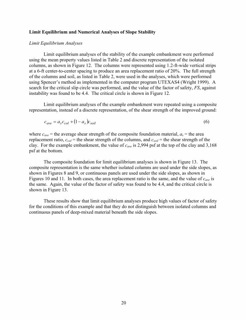
Limit Equilibrium Analyses Limit equilibrium analyses of the stability of the example embankment were performed

using the mean property values listed in Table 2 and discrete representation of the isolated columns, as shown in Figure 12. The columns were represented using 1.2-ft-wide vertical strips at a 6-ft center-to-center spacing to produce an area replacement ratio of 20%. The full strength of the columns and soil, as listed in Table 2, were used in the analyses, which were performed using Spencer’s method as implemented in the computer program UTEXAS4 (Wright 1999). A search for the critical slip circle was performed, and the value of the factor of safety, FS, against instability was found to be 4.4. The critical circle is shown in Figure 12.

Limit equilibrium analyses of the example embankment were repeated using a composite

representation, instead of a discrete representation, of the shear strength of the improved ground:

( ) soilscolsave cacac −+= 1 (6)

where cave = the average shear strength of the composite foundation material, as = the area replacement ratio, ccol = the shear strength of the columns, and csoil = the shear strength of the clay. For the example embankment, the value of cave is 2,994 psf at the top of the clay and 3,168 psf at the bottom.

The composite foundation for limit equilibrium analyses is shown in Figure 13. The

composite representation is the same whether isolated columns are used under the side slopes, as shown in Figures 8 and 9, or continuous panels are used under the side slopes, as shown in Figures 10 and 11. In both cases, the area replacement ratio is the same, and the value of cave is the same. Again, the value of the factor of safety was found to be 4.4, and the critical circle is shown in Figure 13.

These results show that limit equilibrium analyses produce high values of factor of safety

for the conditions of this example and that they do not distinguish between isolated columns and continuous panels of deep-mixed material beneath the side slopes.

21

1v 18 ft Embankment

28 ft Soft Clay

10 ft Dense Sand

2h

Figure 12. Limit equilibrium slope stability analyses using discrete columns.

18 ft Embankment

28 ft Soft Clay

10 ft Dense Sand

2h

Composite Material

1v

Figure 13. Limit equilibrium slope stability analyses using a composite foundation

22

Numerical Analyses If isolated columns are used to support the embankment, as shown in Figure 8, possible

failure modes include composite shear, column bending, and column tilting. Limit equilibrium analyses only address the composite shearing failure mode. Consequently, limit equilibrium analyses can substantially overestimate the stability of column-supported embankments. For example, if the embankment is supported on very strong but small columns at a wide spacing, limit equilibrium analyses of composite shearing could produce a high value of the factor of safety due to the high shear strength of the columns. In reality, the columns could tilt, or they could bend and break, before they shear. Because numerical stress-strain analyses of stability allow for multiple failure modes, including composite shearing, column bending, and column tilting, they are more realistic for high strength columns.

The factor-of-safety, fos, procedure in the numerical analysis program FLAC was applied

to the profile shown in Figure 8 using the mean material property values listed in Table 2, and the value of factor of safety against instability was found to be 1.4, which is substantially lower than the value of 4.4 found from limit equilibrium analyses. Figure 14 shows some of the results from the FLAC analyses, including the shear strains that developed in the soil and tensile failure that developed in the columns. In the numerical analyses, the columns bent and broke, and the soil between the columns experienced shear distortions as the broken part of the columns tilted. Elongation of the upper part of the columns associated with shear distortion of the soil between columns produced tensile failure in the columns, particularly near the toe of the slope.

Shear in soil Tension failure in columns

Figure 14. Results of numerical analyses of the embankment supported on isolated columns

23

The factor-of-safety, fos, procedure in FLAC was also applied to the profile shown in Figure 10, which incorporates panels of deep-mixed material under the embankment side slopes. Panels are constructed by overlapping columns of deep-mixed material. Multiple axis mixing rigs are often used in such applications. In areas where partially hardened material is remixed, CDIT (2002) and Broms (2003) recommend using reduced column strength in the overlapped areas. When multiple-axis equipment is used to construct panels, the zones of reduced strength will be at a spacing corresponding to two or more times the thickness of the panels. Figure 10 shows a panel with vertical joints whose strength is half the value used for the rest of the deep-mixed material. This reduction is in line with the recommendations in CDIT (2002) and Broms (2003).

In two-dimensional FLAC analyses, all the properties of the soil and the deep-mixed

material at the panel location are composite values determined in the same way that the composite strength is determined using Eq. (6). The result of the FLAC fos analysis using the mean property values in Table 2 is a factor of safety value of 3.1 for the embankment with panels under the side slopes. This value is higher than the value of 1.4 determined for isolated columns because the panels serve as shear walls that are not subject to bending like isolated columns are. However, “racking” of the panels can occur by vertical shearing in the weaker joints. This failure mode produces a factor-of-safety value that is lower than the value of 4.4 from the limit equilibrium analyses. Shear that occurs in the numerical analysis of the panel-supported embankment is shown in Figure 15.

Contours indicate high shear strains

Figure 15. Results of numerical analyses of the embankment supported with panels under the

side slope

24

Reliability Analyses of Slope Stability The Taylor Series Method, the Point Estimate Method, the Hasofer-Lind Method, and the

Direct Integration Method, as described in the Methods section and Appendix D of this report, were each employed to determine the probability of failure, p(f), using both limit equilibrium and numerical stress-strain analysis methods. The first three methods are approximate simplified methods, and the Direct Integration Method is an exact method to which the results of the simplified methods were compared. Three parameter values were varied in the reliability analyses: the strength of the columns, the strength of the soft clay between columns, and the friction angle of the embankment fill. Preliminary studies indicated that variations in other parameter values do not have an important influence on the probability of failure for the example embankment.

The values of coefficient of variation that were used in these reliability analyses are 50%

for the column strength, 30% for the undrained shear strength of the clay, and 10% for the friction angle of the embankment (Harr 1987, Duncan and Wright 2005, Navin and Filz 2006b). It was assumed that column strength was lognormally distributed, while clay and embankment strength were normally distributed (Lacasse and Nadim 1996, Navin and Filz 2006b).

The results of the reliability analyses for the embankment supported entirely on isolated

columns are in Tables 3 through 7. The results for reliability analyses for the embankment supported on continuous panels under the side slopes and isolated columns under the full height are in Tables 8 through 10. The results for both cases are summarized in Table 11, which shows the following:

• For the embankment supported on isolated columns everywhere, the numerical analyses

produce a much lower value of the factor of safety than produced by the limit equilibrium analyses. This occurs because the numerical analyses permit realistic failure modes that the limit equilibrium analyses do not permit, such as column bending and tilting.

• Even though the factor of safety from the numerical analyses for the embankment supported everywhere on isolated columns is within the range normally considered acceptable for many roadway embankments, i.e., 1.4, the probability of failure according to the Direct Integration Method is about 3.2 percent, which is unacceptably high. This demonstrates that customary values of the factor of safety are not appropriate for complex systems like column-supported embankments that incorporate materials with high inherent variability and the potential for brittle failure in tension.

• For the embankment supported on panels under the side slopes, the values of factor of safety are high and the probability of failure is low for numerical stress-strain analyses. This demonstrates the value of continuous panels under the side slopes compared to isolated columns at the same area replacement ratio.

• The Hasofer-Lind Method is in better agreement with the Direct Integration Method than is either the Taylor Series Method or the Point Estimate Method. Because the Hasofer-Lind Method provides the best overall agreement of the simplified methods with the Direct Integration Method, the Hasofer-Lind Method is recommended for application to column-supported embankments in practice.

25

Table 3. Taylor Series analyses for embankment supported on isolated columns everywhere Numerical Stress - Limit Equilibrium

Case ccol cclay φemb Strain Analysis Analysis(psi) (psf) (degrees) F ∆F F ∆F

Mean Values 100 0.23*p 35 1.39 4.35Mean - 1σ ccol 50 0.23*p 35 1.35 0.050 2.66 3.362Mean + 1σ ccol 150 0.23*p 35 1.4 6.02Mean - 1σ cclay 100 0.161*p 35 1.24 0.270 4.10 0.484Mean + 1σ cclay 100 0.299*p 35 1.51 4.59Mean - 1σ φemb 100 0.23*p 31.5 1.29 0.190 4.32 0.049Mean + 1σ φemb 100 0.23*p 38.5 1.48 4.37

σF = 0.167 σF = 1.699VF = 0.120 VF = 0.391

β = 2.34 β = 1.97p(f) = 0.97% p(f) = 2.4%βLN = 2.69 βLN = 3.71p(f) = 0.36% p(f) = 0.010%

Normal

Lognormal

Table 4. Point Estimate analysis of embankment supported on isolated columns everywhere using limit equilibrium analysis

qu,col cclay φemb

(psi) (psf) (degrees) F p F*p p*F2

50 0.161*p 31.5 2.41 0.125 0.301 0.724150 0.161*p 31.5 5.79 0.125 0.724 4.18850 0.299*p 31.5 2.85 0.125 0.356 1.012150 0.299*p 31.5 6.22 0.125 0.777 4.83450 0.161*p 38.5 2.44 0.125 0.305 0.745150 0.161*p 38.5 5.82 0.125 0.727 4.22850 0.299*p 38.5 2.91 0.125 0.363 1.056150 0.299*p 38.5 6.27 0.125 0.784 4.911

average 4.34 sum 4.34 21.70σF = 1.701β = 1.96

p(f)= 2.5%

26

Table 5. Point Estimate analysis of embankment supported on isolated columns everywhere using numerical, stress-strain analysis

qu,col cclay φemb

(psi) (psf) (degrees) F p FS*p p*F2

50 0.161*p 31.5 1.13 0.125 0.141 0.160150 0.161*p 31.5 1.15 0.125 0.144 0.16550 0.299*p 31.5 1.37 0.125 0.171 0.235150 0.299*p 31.5 1.40 0.125 0.175 0.24550 0.161*p 38.5 1.26 0.125 0.158 0.198150 0.161*p 38.5 1.33 0.125 0.166 0.22150 0.299*p 38.5 1.57 0.125 0.196 0.308150 0.299*p 38.5 1.63 0.125 0.204 0.332

average 1.36 sum 1.36 1.86σF = 0.168β = 2.11

p(f)= 1.7%

Table 6. Hasofer-Lind analysis of embankment supported on isolated columns everywhere using limit equilibrium analysis

Random input parametersµ σ Distribution (N, LN)

Column cohesion (psi) 100 50 LNEmbankment φ (degrees) 35 3.5 N

Clay cohesion (psf) 324.2 97.26 NStage 1 - Find performance function

Step 1 Step 2 Step 3 Step 4filename: FORMex1 FORMex2 FORMex3 FORMex4

trial β 3 2.5 2.889 2.88Column cohesion (psi) 21.68 27.46 22.85 22.95

Embankment φ (degrees) 24.50 26.25 24.89 24.92Clay cohesion (psf) 32.42 81.05 43.22 44.09

F 0.924 1.265 0.994 1.000Stage 2 - Determine gradients

Step 1 Step 2 Step 3 Step 4 Step 5 Step 6filename: FORMex5 FORMex6 FORMex7 FORMex8 FORMex9 FORMex10

Column cohesion (psi) 20.65 25.24 22.95 22.95 22.95 22.95Embankment φ (degrees) 24.92 24.92 22.43 27.41 24.92 24.92

Clay cohesion (psf) 44.09 44.09 44.09 44.09 39.68 48.50F 0.919 1.079 0.991 1.008 0.988 1.011

Stage 3 - Find performance functionStep 1 Step 2 Step 3 Step 4

filename: FORMex11 FORMex12 FORMex13 FORMex14trial β 2.88 3.5 4.045 4.069

Column cohesion (psi) 28.95 22.71 18.34 18.17Embankment φ (degrees) 34.74 34.68 34.63 34.63 Output

Clay cohesion (psf) 167.78 134.10 104.50 103.20 β= 4.07F 1.547 1.256 1.011 1.001 p(f)= 0.0024%

27

Table 7. Hasofer-Lind analysis of embankment supported on isolated columns everywhere using numerical, stress-strain analysis




Step 1 Step 2 Step 3filename: FORMex1 FORMex2 FORMex3

trial β 1 1.7 1.412Column cohesion (psi) 55.77 40.07 45.91

Embankment φ (degrees) 31.50 29.05 30.06Clay cohesion (psf) 226.94 158.86 186.87

F 1.10 0.93 1.00Stage 2 - Determine gradients

Step 1 Step 2 Step 3 Step 4 Step 5 Step 6filename: FORMex4 FORMex5 FORMex6 FORMex7 FORMex8 FORMex9



Stage 3 - Find performance functionStep 1 Step 2 Step 3 Step 4 Step 5

filename: FORMex10 FORMex11 FORMex12 FORMex13 FORMex14trial β 1.412 1.7 1.947 1.996 1.972

Column cohesion (psi) 77.53 75.31 73.45 73.09 73.26Embankment φ (degrees) 33.82 33.58 33.38 33.33 33.35 Output

Clay cohesion (psf) 194.11 167.58 144.82 140.31 142.52 β= 1.97F 1.13 1.06 1.01 0.99 1.00 p(f)= 2.4%

Table 8. Taylor Series analyses for embankment supported on panels under the side slopes Numerical Stress - Limit Equilibrium

Case ccol cclay φemb Strain Analysis Analysis(psi) (psf) (degrees) F ∆F F ∆F

Mean Values 100 0.23*p 35 3.12 4.35Mean - 1σ ccol 50 0.23*p 35 2.24 1.450 2.66 3.362Mean + 1σ ccol 150 0.23*p 35 3.69 6.02Mean - 1σ cclay 100 0.161*p 35 2.87 0.480 4.10 0.484Mean + 1σ cclay 100 0.299*p 35 3.35 4.59Mean - 1σ φemb 100 0.23*p 31.5 3.01 0.210 4.32 0.049Mean + 1σ φemb 100 0.23*p 38.5 3.22 4.37

σF = 0.771 σF = 1.699VF = 0.247 VF = 0.391

β = 2.75 β = 1.97p(f) = 0.30% p(f) = 2.4%βLN = 4.55 βLN = 3.71p(f) = 0.0003% p(f) = 0.010%

Normal

Lognormal

28

Table 9. Point Estimate analysis of embankment supported on panels under the side slope using numerical, stress-strain analysis

qu,col cclay φemb

(psi) (psf) (degrees) F p F*p p*F2

50 0.161*p 31.5 2.00 0.125 0.250 0.500150 0.161*p 31.5 3.28 0.125 0.410 1.34550 0.299*p 31.5 2.38 0.125 0.298 0.708

150 0.299*p 31.5 3.83 0.125 0.479 1.83450 0.161*p 38.5 2.09 0.125 0.261 0.546

150 0.161*p 38.5 3.54 0.125 0.443 1.56650 0.299*p 38.5 2.47 0.125 0.309 0.763

150 0.299*p 38.5 4.08 0.125 0.510 2.081average 2.96 sum 2.96 9.34

σF = 0.767β = 2.55

p(f)= 0.53%

Table 10. Hasofer-Lind analysis of embankment supported on panels under the side slopes using numerical, stress-strain analysis




Step 1 Step 2 Step 3filename: FORMex1pj3 FORMex2pj3 FORMex3pj3

trial β 3 2.5 2.621Column cohesion (psi) 21.68 27.46 25.93

Embankment φ (degrees) 24.50 26.25 25.83Clay cohesion (psf) 32.42 81.05 69.28

F 0.78 1.07 1.00Stage 2 - Determine gradients

Step 1 Step 2 Step 3 Step 4 Step 5 Step 6filename: FORMex5pj3 FORMex6pj3 FORMex7pj3 FORMex8pj3 FORMex9pj3 FORMex10pj3



Stage 3 - Find performance functionStep 1 Step 2 Step 3 Step 4

filename: FORMex11pj FORMex12pj FORMex13pj FORMex14pjtrial β 2.621 3.6 3.689 3.719

Column cohesion (psi) 31.53 21.36 20.62 20.37Embankment φ (degrees) 34.68 34.56 34.55 34.55 Output

Clay cohesion (psf) 187.03 135.79 131.13 129.56 β= 3.72F 1.48 1.04 1.01 1.00 p(f)= 0.010%

29

Table 11. Summary of reliability analyses for slope stability

Analysis Limit Equilibrium Numerical Analysis of Isolated Columns

Numerical Analysis of Panels

Factor of Safety 4.4 1.4 3.1 Direct Integration, p(f) 0.01% 3.2% 0.009% Taylor Series LN, p(f) 0.01% 0.36% 0.0003% Taylor Series N, p(f) 2.4% 1.0% 0.30% Point Estimate, p(f) 2.5% 1.7% 0.53% Hasofer-Lind, p(f) 0.002% 2.4% 0.01%

The effect of spatial variation in column strength on probability of failure was also investigated (Navin and Filz 2006b). Using an autocorrelation distance of 36 ft, the reliability analyses were repeated, and the results showed little effect on the probability of failure determined from numerical analyses. Spatial variation did reduce the probability of failure determined from limit equilibrium analyses, but this is not of major importance because the failure mechanics are not well represented by limit equilibrium analyses for the conditions of the example embankment.

Parameter Study on Column Strength

The columns in the example problem have a shear strength of 100 psi, which corresponds

to an unconfined compressive strength of 200 psi. A strength of this magnitude is easily achieved using the wet method of deep mixing in many soils. With this strength, the factor-of-safety value computed using numerical analyses was much lower than with limit equilibrium analyses for the embankment supported everywhere on isolated columns. This indicates that numerical methods are needed, at least for strong columns, to perform meaningful stability analyses. For sufficiently low column strengths, it would be reasonable to presume that limit equilibrium analyses may give results similar to numerical analyses.

To determine if such a threshold exists, comparative limit equilibrium analyses and

numerical stress-strain analyses were performed using a second embankment that was similar to the previous example embankment supported on isolated columns everywhere. This second example had a clay layer thickness of 23 ft, the clay shear strength was set equal to 400 psf, and the unconfined compressive strength of the columns varied over the range from about 10 psi to 58 psi. The ratio of factor of safety from limit equilibrium analyses to factor of safety from numerical analyses, FSLE/FSNM, is plotted versus unconfined compressive strength, qu, of the columns in Figure 15. It can be seen that the ratio of FSLE to FSNM diverges from unity at a qu value of about 15 psi. This suggests that, for the conditions analyzed, limit equilibrium methods are suitable only for very low column strengths.

Similar data from Han et al. (2005) are also included in Figure 16. Han et al. (2005)

performed FLAC plane strain analyses of a 16.4 ft high embankment with a 2 horizontal to 1 vertical side slope. The embankment was founded on 32.8 ft of soft clay overlying 6.6 ft of firm soil. The soft clay was improved with 3.3 ft wide strips of deep mixed columns at a replacement ratio of 40 percent. The deep-mixed column strips are located beneath the full width of the

30

embankment and extend 8.2 ft beyond the toe. The strips extend from the ground surface down to 3.3 ft into the deeper firm soil. The soft clay and columns are assumed to be φ = 0 materials with cohesion values of 209 psf for the clay and with column strengths varied as shown in Figure 16. The embankment has a friction angle of 30 degrees with no cohesion. Figure 16 shows that the results of limit equilibrium analyses and numerical analyses by Han et al. (2005) also indicate divergence at a column compressive strength of about 15 psi.

0.5

0.75

1

1.25

1.5

0 20 40 60Unconfined Compression Strength of Columns (psi)

FSLE

/ FS

NM

This ResearchHan et al. (2005)

Figure 16. Comparison of limit equilibrium and numerical analyses of slope stability as a

function of unconfined compressive strength of columns.

Reliability Analyses of Extrusion The CDIT (2002) extrusion analysis shown in Figure 1 and Eq. (1) was applied to the

example embankment for the case in which the embankment is supported on panels beneath the side slopes. The result is a factor-of-safety value of 2.18 for a value of kh equal to zero. In this case, the only material parameter value that has a significant impact on the factor of safety is the shear strength of the clay, which was assumed to have a coefficient of variation equal to 0.30. Reliability analyses were performed in the same way as described above for slope stability analyses. The results are presented in Tables 12 through 14 for the Taylor Series Method, the Point Estimate Method, and the Hasofer-Lind Method.

With only one variable, the normal version of the Taylor Series Method and the Point

Estimate Method result in the same standard deviation of F, and the differences in β and p(f) values between the two methods is only due to the difference between F calculated with mean values in the Taylor Series Method and the average of F calculated using a clay cohesion above and below the mean in the Point Estimate Method. For one variable, the Hasofer-Lind Method reduces to the probability of having a cohesion value less than 154.5 psf, which is the limit state where F equals 1.0. In this case with only one random variable, the Hasofer-Lind method results in the same p(f) value as the Direct Integration Method. It can be seen in Table 14 that the probability of failure is 4%, which is a very high value. The probability of extrusion failure

31

could be reduced by reducing the space between panels, and it could be eliminated by constructing additional panels oriented parallel to the embankment centerline to block extrusion. However, the authors believe that the CDIT (2002) extrusion analysis may be excessively conservative because it doe not take into account arching effects in the clay at the ends of the panels. Such arching effects would be expected to reduce the value of the active earth force, Pa, and increase the value of the passive earth force, Pp, in Eq. (1). It would be worthwhile to develop a revised method for extrusion analyses.

Table 12. Taylor Series Method for extrusion

clay cu

Case (psf) FS ∆FSMean Values 324 2.18

Mean - 1σ cclay 226.8 1.46 1.58Mean + 1σ cclay 421.2 3.04

σF = 0.788VF = 0.362

β = 1.49

p(f) = 6.77%βLN = 2.04

p(f) = 2.07%

Normal

Lognormal

Table 13. Point Estimate Method for extrusion cclay

(psf) F p F*p p*F2

226.8 1.46 0.5 0.730 1.065421.2 3.04 0.5 1.518 4.608average 2.25 sum 2.25 5.67

σF = 0.788β = 1.583

p(f)= 5.7%

32

Table 14. Hasofer-Lind Method for extrusion Random input parameters

µ σ Distribution (N, LN)Clay cohesion (psf) 324.2 97.26 N

Stage 1 - Find performance function1.745

Step 1 Step 2 Step 3trial β 2 1.8 1.745

Clay cohesion (psf) 129.68 149.13 154.48F 0.856 0.969 1.001

Stage 2 - Determine gradientsStep 1 Step 2

Clay cohesion (psf) 139.03 169.93F 0.910 1.094

Stage 3 - Find performance functionStep 1

trial β 1.745 OutputClay cohesion (psf) 154.48 β= 1.75

F 1.001 p(f)= 4.05%

Statistically Based Specifications A principal recommendation of this report is that embankments supported on deep-

mixing-method columns should be designed using reliability analyses. If this is done, then the coefficient of variation used in the reliability analyses can also be used to rationally establish the acceptance criteria in the contract documents for strength of deep mixed columns. Two approaches are considered here. The first approach is based on subareas, or parcels, of the project site. The second approach is based on daily production per mixing rig. After presenting each approach, comments about statistically based specifications and the importance of active involvement of the engineer during construction are provided.

In both approaches, the shear strength used in design should be related to the unconfined

compressive strength that will be measured in the laboratory on specimens obtained from the field. As discussed above in the section that presents the results of the literature review, the residual compressive strength of confined deep mixed material is about 80% of the peak unconfined compressive strength. Using this finding, a conservative strength envelop based on total normal stresses for short term loading is obtained by setting (1) the cohesion intercept equal to 40% of the unconfined compressive strength, i.e., 80% of half the unconfined compressive strength, (2) the friction angle equal to zero, and (3) the tensile strength equal to zero. Thus, the unconfined compressive strength that corresponds to the design shear strength of the deep mixed material is equal to 2.5 times the design shear strength.

Parcel Approach

In the parcel approach, the project site is divided into approximately square parcels about

2,500 ft2 in plan area. This parcel size is based on an autocorrelation distance of 50 ft, which is within the range of autocorrelation distances from 40 to 60 ft that were found at three deep mixing projects in the U.S., as described above. For a particular project, the parcel size could

33

range from about 1,500 ft2 to 4,000 ft2, with larger parcel sizes being appropriate for projects with relatively uniform subsurface conditions, low consequences of failure, and/or successful precedent using deep mixing. After the deep mixed element locations have been established and the parcel size has been determined, the parcels should be drawn on the project plans to facilitate record keeping.

Within each parcel, three elements are selected at random by the engineer, and each of

the selected elements is cored within 28 days after mixing. An element is defined as a single column installed by a single-axis rig or a group of overlapping columns installed by a single set-up of a multi-axis rig. It is recommended that the contractor be made responsible for coring. The core is logged, properly sealed and packaged, and stored in a humid room. For elements that are not longer than about 25 ft, the engineer selects 5 specimens from each cored element for testing in unconfined compression. For longer elements, the number of specimens from each cored element should increase by one for each 5-ft increase in element length. Thus, 8 specimens would be selected from each cored element for 40-ft long elements. The specimens should be tested in unconfined compression approximately 28 days after mixing. For elements that are about 25 ft long, this produces 15 values of unconfined compressive strength for each parcel.

The specifications are written to require that test results meet or exceed the 60%, 80%,

and 95% strengths, as obtained from Figure 17 based on the coefficient of variation used in project design. Accordingly, if 15 strength values are generated, 9 of the samples must meet or exceed the 60% strength, 12 of the samples must meet or exceed the 80% strength, and they must all meet or exceed the 95% strength.

0

20

40

60

80

100

0.0 0.2 0.4 0.6 0.8 1.0Coefficient of Variation

Per

cent

of M

ean

Stre

ngth

(%)

60%

Percent Passing

95%

80%

Figure 17. Required strengths expressed as a percent of the mean strength used in design, for a

lognormal variation of strength values For example, suppose that reliability analyses are performed to design a column-

supported embankment at a particular project site using a value of the coefficient of variation, V, equal to 0.6, and it is found that a mean (average) value of the shear strength of the deep mixed

34

material equal to 80 psi is needed to produce a safe and reliable embankment with a particular area replacement ratio and deep-mixed column layout. This value of shear strength corresponds to an unconfined compression strength equal to 160 psi for a “phi-equals-zero” representation of the deep-mixed material. However, as discussed above and in the Recommendations section, this value should be increased to account for the decrease from the peak unconfined strength to the confined residual strength of deep-mixed material. Thus, the desired mean value of the unconfined compressive strength of the field-mixed material is 2.5 times 80 psi, which equals 200 psi. Now, according to Figure 17 for a coefficient of variation equal to 0.6, the 60%, 80%, and 95% strength values are equal to 76%, 55%, and 34%, respectively, of the mean value. Thus, for 25-ft long elements, the specifications would be written to require that at least 9 of the 15 strength test results for each parcel must meet or exceed 152 psi, at least 12 of the strength test results must meet or exceed 110 psi, and all 15 of the strength test results must meet or exceed 68 psi. In the event that these criteria are not satisfied, the specifications would require that the contractor either (1) perform additional coring on elements selected by the engineer or (2) install additional suitable columns or take other remedial measures approved by the engineer. If the contractor chooses the first option, the same testing procedures and specification values would be applied to determine whether the total set of test results for the parcel satisfy the 60%, 80%, and 95% strength values. The total set of test results includes the initial 15 test results. For example, if two more elements are cored, this produces 10 more test results for a total of 25 test results for that parcel. In this case, at least 15 of the test results must meet or exceed 152 psi, at least 20 of the test results must meet or exceed 110 psi, and at least 24 of the strength test results must meet or exceed 68 psi.

Approach Based on Daily Production per Mixing Rig

In this approach, one deep-mixed element is selected at random by the engineer from the

elements produced each day by each deep mixing rig. The selected element is cored within 28 days after mixing. Again, it is recommended that the contractor be made responsible for coring. The core is logged, properly sealed and packaged, and stored in a humid room. For elements that are not longer than about 25 ft, the engineer selects 5 specimens from each cored element for testing in unconfined compression. For longer elements, the number of specimens should increase by one for each 5-ft increase in element length. The specimens should be tested in unconfined compression approximately 28 days after mixing. For 25-ft long elements, this produces 5 values of unconfined compressive strength for each day’s production by each mixing rig.

The specifications are written to require that test results meet or exceed the 60%, 80%,

and 95% strengths, as obtained from Figure 17 based on the coefficient of variation used in project design. Accordingly, if 5 strength values are generated, 3 of the samples must meet or exceed the 60% strength, 4 of the samples must meet or exceed the 80% strength, and all 5 of the samples must all meet or exceed the 95% strength. Following the example used above, this means that the specifications would be written to require that 3 of the strength test results must meet or exceed 152 psi, at least 4 of the strength test results must meet or exceed 110 psi, and all 5 of the strength test results must meet or exceed 68 psi. In the event that these criteria are not met, the same type of options as described above for the parcel approach would apply.

35

Comments about Statistically Based Specifications The principal benefits of statistically based specifications are that they reflect the real

variability of deep-mixed material, and they achieve the design intent without imposing excessively restrictive requirements on the minimum strength of the deep-mixed material. The approach based on daily production per mixing rig is similar to the approach used by VDOT for the I-95/Route 1 project, and it is easy to apply. The approach based on parcels is more true to the observed spatial variation of deep-mixed material strength and the performance goals of embankments supported on deep-mixed columns, but it does require more involved record keeping to identify elements, cores, and samples within parcels.

In both approaches, statistically based specifications are not meant to replace the active

involvement of the engineer during construction. For example, if the contractor changes mixture proportions or mixing techniques, such changes will produce variations in strength that have controllable causes and are not random. Statistically based specifications make sense for groups of elements for which mix proportions and mixing procedures are uniform. If some elements are suspect because atypical mix proportions or construction procedures were used, it is legitimate for the contract documents to require that such elements be cored and tested.

Furthermore, if subsurface conditions vary across the construction site, this should be

taken into account during reliability based design and when establishing statistically based specifications. For example, if the subsurface explorations establish that organic soil exists within a well-defined zone, but elsewhere the soil is relatively uniform and inorganic, then separate parcels could be established for the organic and inorganic zones. Parcel definition could involve elevation as well as plan-view position.

If conditions encountered during construction are different from those upon which the

design is based, it would be wrong to blindly apply the design and specifications that were developed before the differing conditions became known. In this case, the differing conditions must be confronted directly, and this may require re-design and a change order.

These examples highlight the fact that statistically based specifications are not a

replacement for careful observations and active involvement by the engineer during construction.

DISCUSSION This research shows that failure mechanisms like column tilting and bending can cause

embankment failure at lower load levels than would induce composite shearing through the columns and soft ground. Limit equilibrium methods, as currently employed in engineering practice, do not capture tilting and bending failure modes, and they are not safe for analysis of embankments supported on strong columns. For this reason, numerical analyses of slope stability are needed to capture the realistic failure modes that can control embankment performance and for which there is no practical alternative at present.

36

A related benefit of numerical analyses is that, if properly performed, they also capture the potential for block sliding and bearing capacity failure. Current practice is to perform separate analyses for these failure modes using approximate analytical models (e.g., CDIT 2002). With properly conducted and well interpreted numerical analyses, a single analysis method can address all these aspects of system performance. In order to properly perform such analyses, special care must be devoted to idealization of soil stratigraphy, soil material characterization, and numerical modeling details, as discussed further in Appendix D.

This research also shows that reliability analyses are a necessary component of design for

embankments supported on columns installed by the deep mixing method. The strength of deep-mixed materials is quite variable, and reliability analyses permit this variability to be rationally incorporated in the design process. Furthermore, these systems are complex, and typical variations in clay strength, if not accounted for, could induce abrupt bending failure in isolated columns. Consequently, the ordinary values of factor of safety that geotechnical engineers use to develop reliable designs for other embankment systems are not applicable to embankments supported on columns installed by the deep mixing method. For instance, an example embankment supported on isolated columns was analyzed and found to have a factor of safety equal to 1.4. This value would be considered acceptable in many other situations, but reliability analyses using the Direct Integration Method and the Hasofer-Lind Method showed that the example embankment has a probability of failure equal to about 3%, which is excessively high for public transportation applications. This result demonstrates that typical values of the factor of safety are not adequate for judging acceptability of these systems, and reliability analyses are needed.

Another benefit of reliability analyses is that the coefficient of variation used to design

the embankments can also be used to write a statistically based specification. Such specifications have great potential to reduce construction disputes because they avoid specification of unrealistically high minimum strengths while still fully meeting the design intent.

The numerical and reliability analysis procedures discussed in this report were applied to

deep-mixing-method columns, but the procedures should also be relevant and applicable to vibro-concrete columns, which, like deep-mixing-method columns, have the characteristics of being much stronger than the surrounding soil and having low tensile capacity.

CONCLUSIONS The following conclusions can be drawn from this research:

• The coefficient of variation of unconfined compressive strength for 13 data sets from nine deep mixing projects in the U.S. ranges from 0.34 to 0.79 and has an average value of about 0.57. After removing the variation due to controllable trends of age and water-to-cement ratio of the slurry, the coefficient of variation ranges from 0.17 to 0.67 and has an average value of about 0.4.

• The autocorrelation distance ranged from 40 to 60 ft for three wet-mixing-method projects.

37

• The value of E50/qu is about 300 for soil-cement mixtures created by the wet method using either single or multiple augers.

• Limit equilibrium analyses do not reflect important potential failure mechanisms, such as column tilting and bending. These failure mechanisms are captured in properly conducted numerical analyses.

• The numerical analysis procedures recommended here have been successfully verified against the I-95/Route 1 case history and two sets of centrifuge model tests.

• For embankments supported on deep-mixing-method columns, two-dimensional analyses produce about the same lateral deflections as three-dimensional analyses at the same area replacement ratio and the same column modulus.

• Numerical analyses demonstrate the substantial beneficial effects on stability of continuous panels compared to isolated columns beneath the side slopes of embankments.

• Values of factor of safety that are typically used for design of embankments on unimproved ground, e.g., about 1.4 to 1.5, are too small for embankments supported on deep-mixing-method columns when mean parameter values are used in the analyses.

• Reliability analyses are needed to rationally account for (1) the significant variability of deep-mixed materials and (2) the impact that other changes in system parameters have on the abrupt tensile failure that can occur in deep-mixed materials.

• The Hasofer-Lind Method was found to be more accurate than either the Taylor Series or Point Estimate Methods of reliability analysis.

• Reliability-based design permits rational development of statistically based specifications, which are expected to reduce contract administration problems.

RECOMMENDATIONS For embankments founded on driven piles and stone columns, the limit equilibrium

stability analysis procedures described in Appendices A and B are recommended. For embankments founded on deep-mixing-method columns, VDOT engineers and their

consultants should use the numerical stress-strain and reliability analysis procedures described in this report to evaluate stability. Details of the recommended numerical analysis procedures are presented in Appendix C. Details of reliability analysis procedures are presented in Appendix D, including the Hasofer-Lind Method, which is recommended for reliability analyses of column-supported embankments in practice. Spreadsheets to perform reliability calculations are available from VTRC and the authors.

A value of coefficient of variation, V, of the deep-mixed material in the range of 0.4 to 0.7 can be used in the reliability analyses. This range is based on values in the published literature, as well as analyses of the deep-mixing data sets described in this report. Typical values of V for strength parameters for other geotechnical materials can be found in the literature (e.g., Harr 1987, Duncan 2000). Reliability analyses should be used to produce designs with appropriately low values of the probability of failure, p(f). The design value of p(f) for a particular project will depend on prevailing practice, the consequences that could occur due to failure, and the policies and

38

objectives of the project owner. The U.S. Army Corps of Engineers (1995) provides guidance for selecting an appropriate values of the probability of failure, p(f). The Corps’ guidance is presented in Table D-1, which indicates that a probability of failure equal to 0.1% corresponds to an “above average” level of expected performance. The designer should realize that achieving appropriately low values of p(f) for embankments supported on deep-mixing-method columns will require higher values of factor of safety, when using mean parameter values, than are customarily applied for design of embankments on unimproved ground.

In order to establish realistic values of the unconfined compressive strength of the field

mixed material for a particular project, the engineer should begin by speaking with deep mixing contractors to get an idea of (1) the range of amendment dose rates that can be achieved with available construction equipment at a reasonable cost and (2) the relationship between the strength of laboratory mixed specimens and field mixed materials that can be expected for soil conditions similar to those at the project site. The designer should also perform a laboratory mix design study using soils obtained from the project site. As mentioned previously, the strength of field mixed and cured materials may be 20 to 50 percent of the strength of laboratory mixed and cured materials according to EuroSoilStab (2002), and the percentage may be 20 to 100 percent according to CDIT (2002). The designer should also be aware of values of unconfined compression strength that have been specified on other recent projects. The specified strength values for three such projects are described in the Results section of this report. Based on all this information, a range of realistic field strengths can be established.

Because there is not yet widespread agreement on a comprehensive method for strength

characterization for deep-mixed materials, it is recommended that a reasonable but conservative strength envelope should be used for stability analyses. The authors’ recommendations are that (1) the total stress friction angle should be set equal to zero, (2) the total stress cohesion intercept should be set equal to 40 percent of the unconfined compression strength to account for the reduction from peak unconfined strength to residual confined strength, and (3) no tensile strength should be included. Thus, the design shear strength can be multiplied by a factor of 2.5 to obtain the corresponding unconfined compressive strength.

To reflect the variability that occurs in deep mixed material, construction specifications

should be written using 60%, 80%, and 95% strength values. These strength values are expressed as percentages of the mean strength in Figure 17. The recommended procedure to establish strength values for specifications is illustrated in an example in the text following Figure 17.

As for all geotechnical engineering design recommendations, the recommendations

presented here should be applied with sound judgment and careful evaluation of project-specific details, including subsurface conditions, construction methods, contracting practices, loading conditions, and performance requirements.

It is also recommended that further improvements in the state of practice be achieved by

completing research on the following focused topics:

39

• Proper methods for characterizing the strength and stiffness of deep-mixed material should be developed, including consideration of (1) total-stress versus effective-stress strength characterization, (2) tensile strength, (3) ductility as a function of confining pressure, and (4) nonlinear stress-strain response.

• The interactions of horizontal geosynthetic reinforcement with vertical columnar reinforcement on embankment stability should be investigated.

• An improved method for analysis of extrusion of clay soil between parallel panels should be developed.

COSTS AND BENEFITS ASSESSMENT Because the purpose of this research is to develop analysis methods for stability of

column-supported embankments, assessment of the costs and benefits of the methods must be on a qualitative basis. The costs include the time to study, learn, and use the methods. If VDOT decides to perform such analyses in house, there would be costs associated with software acquisition and personnel training. If VDOT hires outside experts to perform the analyses, there would be costs for these services.

The major benefits of the recommended approaches are their improved accuracy and

reliability compared to previous methods which are based primarily on limit equilibrium analyses. By performing numerical analyses, several realistic potential failure mechanisms of the deep mixed columns, such as column shearing, bending, and tilting, can be rationally analyzed. Another benefit of performing numerical analyses is that separate analyses of overall sliding and bearing capacity are not necessary. All these potential modes of system failure are automatically included in properly performed numerical analyses. By combining numerical analyses with reliability analyses, a design can be rationally developed to produce an acceptably low probability of failure without over-designing the system. In addition, statistically based specifications that are developed using the coefficient of variation employed in reliability based design have the potential to reduce construction bid prices, and they are expected to reduce contract administration problems while still satisfying the design intent.

ACKNOWLEDGMENTS

Funding for this research was provided by the Virginia Transportation Research Council, the National Deep Mixing Program, the National Science Foundation, and Virginia Tech’s Center for Geotechnical Practice and Research. The authors recognize the important contributions made by George Burke, Derrick Dassenbrock, Jeff Farrar, Stanley L. Hite, Edward J. Hoppe, Meeok Kim, Jose P. Gomez III, Jie Han, Jim Lambrechts, Ali Porbaha, Thomas E. Pelnik III, Jen Schaeffer, David P. Shiells, Miriam E. Smith, Masaaki Terashi, David Weatherby, Phil Wunderly, and David Yang.

40

REFERENCES

Aboshi, H., Ichimoto, E., Enoki, M., and Harada, K. The "Compozer" - a Method to Improve Characteristics of Soft Clays by Inclusion of Large Diameter Sand Columns. Proceedings of International Conference on Soil Reinforcement. 1979, pp. 211-216.

Ang, A. and Tang, W. Probability Concepts in Engineering Planning and Design: Volume I -Basic Principles. John Wiley and Sons, Inc., New York, 1975.

Ang, A. and Tang, W. Probability Concepts in Engineering Planning and Design: Volume II –Decision, Risk, and Reliability. John Wiley and Sons, Inc., New York, 1984.

Bachus, R. C. and Barksdale, R. D. Design Methodology for Foundations on Stone Columns. Foundation Engineering: Current Principles and Practices, ASCE GSP No. 22. 1989, pp. 244-257.

Baecher, G. and Christian, J. Reliability and Statistics in Geotechnical Engineering. Wiley, West Sussex, 2003.

Baker, S. Deformation Behaviour of Lime/Cement Column Stabilized Clay. Swedish Deep Stabilization Research Centre, Rapport 7, Chalmers University of Technology, 2000.

Barksdale, R. D. and Bachus, R. C. Design and Construction of Stone Columns, Volume 1. Federal Highway Administration, RD-83/026. 1983.

Barksdale, R. D. and Takefumi, T. Design, Construction and Testing of Sand Compaction Piles. Deep Foundation Improvements: Design, Construction, and Testing ASTM STP 1089. 1991, pp. 4-18.

Bowles, J. E. Foundation Analysis and Design, 5th Edition. McGraw-Hill, Inc, New York, 1996.

British Standards Institution. BS8006 Code of Practice for Strengthened/Reinforced Soils and Other Fills. BSI, London, U.K., 1995.

Broms, B. B. Stabilization of slopes with piles. Proceedings of the 1st International Symposium on Landslide Control, 1972, pp. 115-123.

Broms, B. B. Stabilization of Soft Clay in Southeast Asia. Proceedings of the 5th International Geotechnical Seminar on Case Histories in Soft Clay. 1987, pp. 163-198.

Broms, B. B. Deep Soil Stabilization: Design and Construction of Lime and Lime/Cement Columns, Royal Institute of Technology, Stockholm, Sweden, 2003.

Bruce, D. A. An Introduction to the Deep Mixing Methods as Used in Geotechnical Applications - Volume III: The Verification and Properties of Treated Ground. Federal Highways Administration, FHWA-RD-99-167, 2002.

41

Carlsten, P. and Ekstrom, J. Lime and Lime Cement Columns, Guide for Project Planning, Construction and Inspection. Swedish Geotechnical Society, SGF Report 4:95 E . 1997.

CDM (Cement Deep Mixing) Design and Construction Manual for CDM Institute, Partial English Translation, 1985.

CDIT (Coastal Development Institute of Technology) The Deep Mixing Method: Principle, Design and Construction. A.A. Balkema: The Netherlands, 2002.

D’Appolonia, D.J., D’Appolonia, E., and Brisette, R.F. Settlement of Spread Footings on Sand, (closure), Proc. Journal of the Soil Mechanics and Foundations Division, 1970, vol. 96(SM2), pp. 754-761.

Dong, J., Hiroi, K., and Nakamura, K. Experimental Study on Behavior of Composite Ground Improved by Deep Mixing Method under Lateral Load. Grouting and Deep Mixing, Proceedings of IS-Tokyo 96, 2nd International Conference on Ground Improvement Geosystems. Tokyo, 1996, pp. 585-590.

Duncan, J. M. Factors of Safety and Reliability in Geotechnical Engineering. Journal of Geotechnical and Geoenvironmental Engineering, Vol. 126, No. 24, 2000, pp. 307-316.

Duncan, J. M. and Buchignani, A. L. An Engineering Manual for Settlement Studies, Department of Civil Engineering, University of California, 1976.

Duncan, J. M. and Wong, K. S. User’s Manual for SAGE, Vol. II – Soil Properties Manual, Center for Geotechnical Practice and Research, Blacksburg, VA, 1999.

Duncan, J. M. and Wright, S. G. Soil Strength and Slope Stability. John Wiley & Sons, Inc., New Jersey, 2005.

El-Ramly, H., Morgenstern, N., and Cruden, D. Probabilistic Slope Stability Analysis for Practice. Canadian Geotechnical Journal, Vol. 39, No. 24, 2002, pp. 665-683.

Enoki, M., Yagi, N., Yatabe, R., and Ichimoto, E. Shearing Characteristics of Composite Ground and its Application to Stability Analysis. Deep Foundation Improvements: Design, Construction, and Testing, ASTM STP 1089. 1991, pp. 19-31.

EuroSoilStab Development of Design and Construction Methods to Stabilise Soft Organic Soils. Design Guide Soft Soil Stabilization, CT97-0351, Project No.: BE 96-3177, 2002.

Filz, G. M., Hodges, D. E., Weatherby, D. E., and Marr, W. A. Standardized Definitions and Laboratory Procedures for Soil-Cement Specimens Applicable to the Wet Method of Deep Mixing. Innovations in Grouting and Soil Improvement, Reston, Virginia , 2005.

Filz, G. M. and Smith, M. E. Design of Bridging Layers in Geosynthetic-Reinforced, Column-Supported Embankments, Virginia Transportation Research Council, Charlottesville, VA, 2006.

42

Goughnour, R. R., Sung, J. T., and Ramsey, J. S. Slide Correction by Stone Columns. Deep Foundation Improvements: Design, Construction, and Testing, ASTM STP 1089, Philadelphia, 1991, pp. 131-147.

Han, J., Parsons, R. L., Huang. J., and Sheth, A. R. Factors of Safety against Deep-Seated Failure of Embankments over Deep Mixed Columns . Deep Mixing '05: International Conference on Deep Mixing Best Practice and Recent Advances. 2005.

Harr, M. Reliability-based Design in Civil Engineering. McGraw-Hill, New York, 1987.

Hasofer, A. A., and Lind, A. M. An Exact and Invariant Second-Moment Code Format,” Journal of the Engineering Mechanics Division, Vol. 100, 1974, pp. 111-121.

Hayashi, H., Nishikawa, J., Ohishi, K., and Terashi, M. Field Observation of Long-term Strength of Cement Treated Soil. Grouting and Ground Treatment, Proceedings of the 3rd International Conference. New Orleans, 2003, pp. 598-609.

Honjo, Y. A Probabilistic Approach to Evaluate Shear Strength of Heterogeneous Stabilized Ground by the Deep Mixing Method. Soils and Foundations, Vol. 22, No. 24, 1982, pp. 23-38.

Huang, J., Han, J., and Porbaha, A. Two and Three-Dimensional Modeling of DM Columns under Embankments. GeoCongress: Geotechnical Engineering in the Technology Age. 2006.

Inagaki, M., Abe, T., Yamamoto, M., Nozu, M., Yanagawa, Y., and Li, L. Behavior of Cement Deep Mixing Columns under Road Embankments. Physical Modelling in Geotechnics: ICPMG '02, 2002, pp. 967-972.

ITASCA Consulting Group FLAC2D Fast Lagrangian Analysis of Continua, ITASCA Consulting Group, 2002a.

ITASCA Consulting Group FLAC3D Fast Lagrangian Analysis of Continua in 3 Dimensions, ITASCA Consulting Group, 2002b.

Jacobson, J. R., Filz, G. M., and Mitchell, J. K. Factors Affecting Strength Gain in Lime-cement Columns and Development of a Laboratory Testing Procedure, Report prepared for the Virginia Transportation Research Council, Virginia Polytechnic Institute and State University, 2003.

Jacobson, J. R., Filz, G. M., and Mitchell, J. K. Factors Affecting Strength of Lime-Cement Columns Based on a Laboratory Study of Three Organic Soils. Deep Mixing '05: International conference on deep mixing best practice and recent advances, 2005.

Japanese Geotechnical Society Standard Practice for Making and Curing Stabilized Soil Specimens without Compaction (JGS 0821-2000). Geotechnical Test Procedure and Commentary, 2000.

43

Jones, C. J. F. P., Lawson, C. R., and Ayres, D. J. Geotextile Reinforced Piled Embankments. Proceedings, 5th International Conference on Geotextiles, Geomembranes, and Related Products. 1990, pp. 155-160.

Kawasaki, T., Niina, A., Saitoh, S., Suzuki, Y., and Honjyo, Y. Deep Mixing Method using Cement Hardening Agent. Proceedings of the 10th International Conference on Soil Mechanics and Foundation Engineering, Stockholm, 1981, pp. 721-724.

Kitazume, M., Ikeda, T., Miyajima, S., and Karastanev, D. Bearing Capacity of Improved Ground with Column Type DMM. Grouting and Deep Mixing, Proceedings of IS-Tokyo 96, 2nd International Conference on Ground Improvement Geosystems, 1996, pp. 503-508.

Kitazume, M., Okano, K., and Miyajima, S. Centrifuge Model Tests on Failure Envelope of Column Type Deep Mixing Method Improved Ground. Soils and Foundations, Vol. 40, No. 24, 2000, pp. 43-55.

Kivelo, M. Stabilization of Embankments on Soft Soil with Lime/cement Columns. Doctoral Thesis, Royal Institute of Technology, 1998.

Kivelo, M. and Broms, B.B. Mechanical behaviour and shear resistance of lime/cement columns. International Conference on Dry Mix Methods: Dry Mix Methods for Deep Soil Stabilization, 1999, pp. 193-200.

Lacasse, N., Nadim, F. Uncertainties in Characterizing Soil Properties. Uncertainties in the Geologic Environment: From Theory to Practice, Proceedings of Uncertainty ’96, Madison, 1996, pp. 49-75.

Lambrechts, J. R., Ganse, M. A., and Layhee, C. A. Soil Mixing to Stabilize Organic Clay for I-95 Widening, Alexandria, VA. Grouting and Ground Treatment, Proceedings of the 3rd International Conference, New Orleans, 2003, pp. 575-585.

Lambrechts, J.R., Roy, P.A., and Wishart, E. Design Conditions and Analysis Methods for Soil-cement in Fort Point Channel. Design and Construction of Earth Retaining Structures, Proceedings of Sessions of Geo-Congress '98, Reston, Virginia, 1998, pp. 153-174.

Larsson, S. On the use of CPT for Quality Assessment of Lime-cement Columns. Deep Mixing '05: International conference on deep mixing best practice and recent advances, 2005.

Matsuo, O. Determination of Design Parameters for Deep Mixing. Tokyo Workshop 2002 on Deep Mixing, Coastal Development Institute of Technology, 2002, pp. 75-79.

McGinn, A. J. and O'Rourke, T. D. Performance of Deep Mixing Methods at Fort Point Channel. Report to Massachusetts Turnpike Authority, Federal Highway Administration, and Bechtel/Parsons Brinckerhoff, Cornell University, 2003.

McGregor, J. A. and Duncan, J. M. Performance and Use of the Standard Penetration Test in Geotechnical Engineering Practice, Center for Geotechnical Practice and Research, Blacksburg, VA, 1998.

44

Mitchell, J.K., and Gardner, W.S. In-situ measurement of volume change characteristics. State-of-the-art report. Proceedings of the Conference on In-situ Measurement of Soil Properties, Specialty Conference of the Geotechnical Division, North Carolina State University, Raleigh, Vol. II, 1975, pp. 279-345.

Miura, N., Horpibulsuk, S., and Nagaraj, T. Engineering Behavior of Cement Stabilized Clay at High Water Content. Soils and Foundations, Vol. 41, No. 24 , 2002, pp. 33-45.

Navin, M. P. Stability of Embankments Founded on Soft Soil Improved with Deep-Mixing-Method Columns, Ph.D. dissertation, Blacksburg, VA, 2005.

Navin, M. P. and Filz, G. M. Statistical Analysis of Strength Data from Ground Improved with DMM Columns. Deep Mixing '05: International conference on deep mixing best practice and recent advances, 2005.

Navin, M.P. and Filz, G.M. Numerical Stability Analyses of Embankments Supported on Deep Mixed Columns. GeoShanghai International Conference, 2006a.

Navin, M. P. and Filz, G. M. Simplified Reliability-Based Procedures for Design and Construction Quality Assurance of Foundations Improved by the Deep Mixing Method, National Deep Mixing Program, 2006b.

Navin, M. P. and Filz, G. M. Reliability of Deep Mixing Method Columns for Embankment Support. GeoCongress: Geotechnical Engineering in the Technology Age. 2006c.

Ou, C. Y., Wu, T. S., and Hsieh, H. S. Analysis of Deep Excavation with Column Type of Ground Improvement in Soft Clay. Journal of Geotechnical Engineering, Vol. 122, No. 9, 1996, pp. 709-716.

Pannatier, Y. Variowin: Software for Spatial Data Analysis in 2D. Springer-Verlag, New York, 1996.

Porbaha, A., Ghaheri, F., and Puppala, A. J. Soil Cement Properties from Borehole Geophysics Correlated with Laboratory Tests. Deep Mixing '05: International conference on deep mixing best practice and recent advances, 2005.

Poulos, H. G. Simplified design procedures for piled raft foundations. Deep Foundations 2002, 2002, pp. 441-458.

Rosenblueth, E. Point Estimates for Probability Moments, Proceedings of the National Academy of Sciences, Vol. 72, No. 10, 1975.

Shiells, D. P., Pelnik III, T. W., and Filz, G. M. Deep Mixing: an Owner's Perspective. Grouting and Ground Treatment, Proceedings of the 3rd International Conference, New Orleans, 2003, pp. 489-500.

Smith, M. E. and Filz, G. M. Settlement of Column Supported Embankments. VTRC, 2006.

45

Stewart, M. E., Navin, M. P., and Filz, G. M. Analysis of a Column-supported Test Embankment at the I-95/Route 1 Interchange. Proceedings of Geo-Trans 2004, Geotechnical Engineering for Transportation Projects, ASCE, 2004, pp. 1337-1346.

Takenaka, D. and Takenaka, K. Deep Chemical Mixing Method - Using Cement as Hardening Agent. Takenaka Corporation, Tokyo, 1995.

Tatsuoka, F., Kohata, Y., Uchida, K., and Imai, K. Deformation and strength characteristics of cement-treated soils in Trans-Tokyo Bay Highway Project. Grouting and Deep Mixing, Proceedings of IS-Tokyo 96, 2nd International Conference on Ground Improvement Geosystems, Tokyo, 1996, pp. 453-459.

Terashi, M. The State of Practice in Deep Mixing Methods. Grouting and Ground Treatment, Proceedings of the 3rd International Conference, New Orleans, 2003, pp. 25-49.

Terashi, M. Keynote Lecture: Design of deep mixing in infrastructure applications. Deep Mixing '05: International conference on deep mixing best practice and recent advances, 2005.

Ting, W. H., Chan, S. F., and Ooi, T. A. Design Methodology and Experiences with Pile Supported Embankments. Development in Geotechnical Engineering. Balkema, Rotterdam, 419-432. 1994.

Unami, K. and Shima, M. Deep Mixing Method at Ukishima Site of the Trans-Tokyo Bay Highway. Grouting and Deep Mixing, Proceedings of IS-Tokyo 96, 2nd International Conference on Ground Improvement Geosystems, 1996, pp. 777-782.

U.S. Army Corps of Engineers. Introduction to Probability and Reliability Methods for Use in Geotechnical Engineering. Engineering Technical Letter 1110-2-547, Department of the Army, Washington, DC. 1995.

Wright, S. G. UTEXAS4: A Computer Program for Slope Stability Calculations. Shinoak Software, Austin, 1999.

Yang, D. S., Scheibel, L. L., Lobedan, F., and Nagata, C. Oakland Airport Roadway Project. Soil Mixing Specialty Seminar, 26th DFI Annual Conference, 2001.

47

APPENDIX A

STABILITY ANALYSES OF EMBANKMENTS SUPPORTED ON DRIVEN PILES

According to Ting et al. (1994), piles in embankment support applications are designed to carry the full embankment load, and vertical piles are not designed to carry any lateral forces. The lateral resistance of piles beneath embankments is often low, especially in soft soils (Broms 1987). Current practice is to account for possible lateral spreading of the embankment and foundation with either battered piles near the edge of embankments as shown in Figure A-1, or a geosynthetic layer as shown in Figure A-2 (Jones et al. 1990).

Soft Foundation Soils

Figure A-1. Pile-supported embankment with batter piles (after Jones et al. 1990)

Soft Foundation Soils

Geosynthetic Layer(s)

Figure A-2. Pile-supported embankment with geosynthetic reinforcement (after Jones et al. 1990)

A bridging layer consisting of compacted granular soil is often used to distribute the vertical embankment load to piles. Geosynthetic reinforcement may be employed in the bridging layer to enhance load transfer to the piles. Analysis and design of geosynthetic reinforcement for vertical load transfer in bridging layers is described in Filz and Smith (2006). Geosynthetic reinforcement can also be used in the bridging layer to provide tensile capacity to stabilize the embankment side slopes. This tensile capacity can counteract the lateral spreading force that

48

could otherwise cause slope stability problems, potentially eliminating the need for battered piles. Stability analysis of pile-supported embankments with geosynthetic reinforcement can be performed according to the method in BS 8006 (1995). This method assumes a circular failure surface, and the analysis is performed as shown in Figure A-3.

Circle center Xp1

Xp2

Tr

Fp1 Fp2

Y

Figure A-3. Stability analysis of pile-supported embankments (after BS8006 1995)

The vertical forces in the piles, FP1, FP2, etc., are assumed to be equal to the embankment load over the tributary area associated with each pile. The restoring moment due to the pile forces, MRP, is calculated from Eq. (A-1) based on the pile forces and the horizontal distance from the center of the slip circle to the piles, XP1, XP2, etc.

2211 PPPPRP XFXFM += (A-1)

The tension in the geosynthetic reinforcement due to lateral spreading of the

embankment, Tr, is determined according to Eq. (A-2).

HqKHKT aar += 221 γ (A-2)

where: Ka = active earth pressure coefficient γ = unit weight of the embankment material H = full height of the embankment q = surcharge pressure on the embankment surface

49

The geosynthetic reinforcement should be selected to safely carry the tension force, Tr, needed to provide slope stability. If geosynthetic reinforcement is also used to enhance vertical load transfer to the piles, then the required tensile capacity for vertical load transfer, Tv, should be added to Tr to obtain the total required tensile capacity, T, of the geosynthetic reinforcement. The geosynthetic reinforcement should be selected to provide an allowable tension capacity equal to or greater than T in the transverse direction and a tension capacity equal to or greater than Tv in the longitudinal direction of the embankment.

The restoring moment due to the tension in the geosynthetic reinforcement, MRR, is

calculated from Eq. (A-3).

YTM rRR = (A-3) where Y = vertical distance from the center of the slip circle to the geosynthetic reinforcement. The driving moment, MD, and resisting moment, MR, are calculated for the case without piles. The additional resisting moments due to piles, MRP, and geosynthetic reinforcement, MRR, are then added to MR. The factor of safety, FS, of the improved ground is then calculated from Eq. (A-4).

D

RRRPR

MMMMFS ++

= (A-4)

If no geosynthetic reinforcement is used in the embankment, a horizontal force equal to the tension force computed in Eq. (A-2) should be provided by the horizontal component of the axial capacity of battered piles, as shown in Figure A-1. Vertical piles in soft ground under embankments should not be relied upon to carry lateral loads. In order to maintain stability during construction and prevent overstressing piles, Broms (1987) recommends that construction of embankments supported on inclined piles should start at the center of the embankment and proceed simultaneously towards both sides. Ting (1994) states that the Swedish State Road Department (1974) allows the safe structural load of piles in embankment support applications to be 1.5 times that commonly used for buildings.

51

APPENDIX B

STABILITY ANALYSES OF EMBANKMENTS FOUNDED ON STONE COLUMNS

In stability analyses of embankments supported on stone columns, the failure mechanism that is typically assumed is a sliding failure surface that mobilizes the shear strength of the soil and the columns. Two of the three analysis methods described below seek to define an average shear strength that can be applied to the composite ground. The third method represents the soil and the stone columns by alternating vertical strips of material, but the shear surface passes through the columns and the soil, so that composite action is incorporated in this method also. Although composite shearing is the primary failure mode that is considered in slope stability analyses of embankments supported on stone columns, it is worthwhile recognizing that other failure modes can occur. For example, Bachus and Barksdale (1989) indicate that using composite strengths is inappropriate for area replacement ratios less than 20% because weak soil can flow around widely spaced columns. The composite shear strength depends on the shear strength of the soil, the shear strength of the columns, and the area replacement ratio. The shear strength of the columns depends on the stress concentration ratio in the columns. According to Barksdale and Takefumi (1991), the stress concentration ratio equals one immediately after rapid loading and increases as consolidation occurs and load is shifted to the more rigid columns. The stress concentration that develops in the columns as the embankment settles increases the frictional shear resistance of the columns. Use of a bridging layer may increase the stress concentration both immediately following construction and after consolidation. The methods presented here consider the short-term, undrained condition for the soft clay between columns. This is considered to be the critical condition since the edge stability of the embankment should improve over time as consolidation occurs. All of the methods assume a long embankment that is reinforced with stone columns having constant diameter and spacing.

Circular Sliding Surface Method The Circular Sliding Surface Method was developed for sand compaction piles, but it has also been applied to stone columns. The Circular Sliding Surface Method evaluates stability using circular failure surfaces and a composite shear strength. The assumed failure surface is illustrated in Figure B-1.

52

z α

Figure B-1. Circular sliding surface method for granular piles (after Aboshi et al. 1979) The composite shear strength is determined based on a proportionate average of soil strength and stone column strength for a given area replacement ratio and stress concentration ratio (Aboshi et al. 1979). The composite shear strength at any point along the failure surface is obtained from Eq. (B-1). This equation uses undrained strengths for the soil and drained strengths for the column.

( ) ( )[ ] ( ) αφσµγαφσµγτ 22 cos'tan'costan1 colcolcolssoilsoilsoilus zazca ++++−= (B-1) where:

τ = composite shear strength along the sliding surface as = area replacement ratio cu = undrained cohesion intercept of the soil γsoil = total unit weight of the soil z = distance from ground surface to failure surface σ = average applied vertical stress from the embankment µsoil = ratio of stress change in the soil from the embankment load to the average applied

vertical stress from the embankment φsoil = undrained friction angle of the soil = 0 for saturated clay in undrained loading µcol = ratio of stress change in the stone column from the embankment to the average

applied vertical stress from the embankment φ'col = drained friction angle of the column γ 'col = buoyant unit weight of the column α = inclination of the failure surface, as shown in Figure B-1.

The composite shear strength determined from Eq. (B-1) is typically used in conjunction with the Ordinary Method of Slices to determine the stability of the stabilized ground (Enoki 1991).

Average Strength Parameter Method

Similar to the Circular Sliding Surface Method, the Average Strength Parameter Method determines composite shear strength parameters to evaluate stability (Goughnour 1991). The

53

composite cohesion, or average cohesion, is determined based on the cohesion intercept of the soil and the area replacement ratio according to Eq. (B-2).

( )suav acc −= 1 (B-2)

where cav = average cohesion, cu = cohesion intercept of the soil, and as = area replacement ratio.

The composite, or average, friction angle is determined as a weighted average between the friction angle of the soil and the friction angle of the stone columns, and it is influenced by the orientation of the assumed failure surface. The composite friction angle is determined using Eq. (B-3).

( )( )11

tantan1tan−+

+−=

rs

colsrsoilsav Sa

aSa φφφ (B-3)

where φav = average friction angle, φsoil = friction angle for the soil, φcol = friction angle for the column, and Sr = stress ratio applicable to the orientation of the failure surface at that location, which is determined by Eq. (B-4).

α−+= cos) ·(nSr 11 (B-4)

where n = stress concentration ratio = the ratio of the vertical stress in the column to the vertical stress in the soil, and α = inclination of the assumed failure surface.

The composite, or average, unit weight is determined by Eq. (B-5).

( ) colssoilsav aa γγγ +−= 1 (B-5)

where γav = average unit weight, γsoil = unit weight of the soil, and γcol = unit weight of the column. The average parameter values as determined by Eqs. (B-2), (B-3), and (B-5) are then used to evaluate stability by means of existing slope stability analysis methods, such as Bishop’s or Spencer’s methods.

Profile Method The Profile Method is recommended by Barksdale and Bachus (1983) for evaluating the stability of improved ground using computer programs for slope stability analysis. In the Profile Method, the stone columns are replaced by equivalent “strips” in profile, and the composite foundation is simplified as a series of alternating strips of columns and native soil. For example, for the equilateral triangle arrangement of columns shown in Figure B-2, the column strips have a centerline-to-centerline distance of 0.866·s, where s = the center-to-center spacing of the columns. The width, w, of the strips in a two-dimensional representation may be calculated from Eq. (B-6).

54

saw s866.0= (B-6)

where w = width of strips, as = replacement ratio, and s = column spacing.

Firm Bearing Strata

Soil

Fictitious Layer H T

w

γ f soil

γ f col

s

0.866s 0.866s 0.866s

w = 0.866ass

a) Section View

b) Plan View

Figure B-2. Stone column strip idealization (after Barksdale and Bachus 1983)

Within the computer model, a fictitious layer is placed at the interface between the embankment and the foundation to generate stress concentrations in the stone columns. The fictitious layer is assigned no strength, and its thickness, T, should be as small as practical.

55

Barksdale and Bachus (1983) recommend a constant thickness of 0.25 to 0.5 ft beneath the full height of embankment, with the thickness tapering to zero at the toe, as illustrated in Figure B-2. The layer should have a high unit weight in the areas above the stone column strips, and a negative unit weight over the soil strips. The unit weights in the fictitious layer are calculated based on the layer thickness, the stress ratios, and the embankment loading to give the correct load in the columns and the surrounding soil. Eqs. (B-7) and (B-8) are used to determine the unit weights for the fictitious layer (Barksdale and Bachus 1983):

( )T

Hcolcolf

11 γµγ −= (B-7)

( )

THsoilsoil

f11 γµγ −

= (B-8)

where: γf

col = unit weight of the fictitious layer above the stone column γf

soil = unit weight of the fictitious layer above the soil γ1 = unit weight of the embankment H = height of the embankment

Comparison of Stability Analysis Methods The Profile Method is an adaptation of the Circular Sliding Surface Method for use with a computer program for slope stability analysis. For any value of stress concentration ratio, the Profile Method and the Circular Sliding Surface Method give the same result when using the Ordinary Method of Slices (OMS). The Circular Sliding Surface Method of analysis is commonly used in conjunction with OMS to model the composite soil in Japan (Enoki 1991).

The Average Parameter Method is difficult to use with a computer program for slope stability analysis because the average friction angle changes with inclination of the failure surface.

A computational difference between the Circular Sliding Surface Method and the Average Parameter Method relates to the effect of the stress concentration ratio, n. For the Circular Sliding Surface Method, stress concentration in the columns only pertains to the embankment loading. For the Average Parameter Method, stress concentration in the columns pertains to both the embankment loading and the weight of the foundation soils above the sliding surface. According to Barksdale and Takefumi (1990), the stress concentration ratio equals one immediately after rapid loading, and it increases as consolidation occurs. For a stress concentration ratio of one, the Average Parameter Method gives approximately the same result as the other two methods when OMS is used. The only difference, in this situation, is that the shear strength of the soil and the stone columns is calculated based on an average unit weight of the foundation for the Average Parameter Method, and the shear strengths are based on the separate unit weights of the soil and the stone columns for the Circular Sliding Surface Method and the Profile Method.

56

The authors of this report recommend that the Profile Method be used with a computer program for slope stability analysis of embankments supported on stone columns. This permits easy searching for the critical failure surface. For stone columns installed in soft ground, it is most conservative to use a value of the stress concentration ratio, n, equal to one, which corresponds to µsoil = µcol = unity. However, even with rapidly applied embankment loads, the stress concentration ratio is very likely greater than one because the drainage path length for consolidation of the near surface soils is short, which means that some consolidation and stress concentration onto the columns will occur during embankment construction. For values of n greater than one, the corresponding values of µsoil and µcol can be determined from Eqs. (B-9) and (B-10).

( ) ssoil an 11

1−+

=µ (B-9)

( ) scol an

n11 −+

=µ (B-10)

57

APPENDIX C

GUIDELINES FOR NUMERICAL ANALYSES OF EMBANKMENTS SUPPORTED ON DEEP-MIXED COLUMNS

The verification studies described in the main body of this report and in Navin (2005) demonstrate that numerical analysis can effectively match observed behavior of embankments and similar structures founded on soft clay improved with deep-mixed columns. This appendix summarizes key aspects of the numerical analysis procedures that were successfully applied using FLAC. Many of the general principles embodied in these guidelines are also applicable to the analysis of column-supported embankments performed using other numerical analysis software, such as finite element codes. These approaches are also thought to apply to embankments supported on vibro-concrete columns because, like deep-mixed columns, they are stiff columns with low bending and tensile strength.

Material Property Values for the Short-Term, “End-of-Construction” Case Numerical analyses of centrifugal model experiments performed by Inagaki et al. (2002) and the numerical analysis of the VDOT test embankment for the I-95/Route 1 Interchange were performed using water-soil coupled analyses. These analyses employed the Modified Cam Clay Model for the soft clay in the foundation. Further investigations revealed that, for considerations of slope stability immediately after embankment construction, numerical analyses could be successfully performed using much simpler, short-term, “end of construction” analyses with undrained strength parameter values based on total normal stresses for low permeability materials, such as the clay and columns, and drained parameter values based on effective normal stresses for high permeability materials and unsaturated materials, such as sand layers and embankments. The materials in the short-term analyses can be modeled using elastic properties in conjunction with the Mohr-Coulomb failure criterion.

Geotechnical engineers are accustomed to selecting unit weights, as well as the Mohr-Coulomb strength property values of cohesion, c, and friction angle, φ, for soils. In many cases, the elastic properties that are required for soils, i.e., the Young’s modulus, E, and Poisson’s ratio, ν, can be selected based on published values in the literature (e.g., D’Appolonia et al. 1970, Mitchell and Gardner 1975, Duncan and Buchignani 1976, Bowles 1996, McGregor and Duncan 1998, Duncan and Wong 1999, and Poulos 2002). The Poisson’s ratio for saturated clay and columns in short term analyses is nearly 0.5; however, to avoid numerical difficulties, a value lower than 0.5 must be used. For undrained materials in the factor of safety, fos, analyses, a value of ν equal to 0.45 is suitable. Although it is convenient to select values of the elastic properties E and ν, FLAC requires values of the bulk modulus, K, and shear modulus, G. Values of K and G can be determined from E and ν using Eqs. (C-1) and (C-2).

( )ν213 −=

EK (C-1)

58

( )ν+=

12EG (C-2)

Kitazume et al. (1996) clearly observed bending failure in columns during centrifuge

testing. Inagaki et al. (2002) noted that, after centrifuge testing, columns extracted from the model had cracked, and the authors felt this was indicative of bending failure. Both sets of authors performed numerical analysis of their centrifuge tests, but neither group allowed for failure of the columns, which were modeled as linear elastic materials. In order to understand the behavior of columns and the overall stability of these systems, it is necessary to incorporate a failure criterion, like the Mohr-Coulomb criterion, for the columns.

As part of this research, over 7,000 strength measurements were collected from nine

deep-mixing projects around the United States. The data collected in this study, and summarized in the Results section of this report, provide useful information about the strength and modulus values that have been achieved for columns installed by the deep mixing method. Because there is not yet widespread agreement on a comprehensive method for strength characterization for deep-mixed materials, it is recommended that a reasonable but conservative strength envelope should be used for stability analyses. The authors’ recommendations are that (1) the total stress friction angle should be set equal to zero, (2) the total stress cohesion intercept should be set equal to 40 percent of the unconfined compression strength to account for the reduction from peak unconfined strength to residual confined strength, and (3) no tensile strength should be included.

In FLAC, material densities rather than unit weights are the required input, so the user

must convert unit weights to densities by dividing the unit weights by the acceleration of gravity.

Initial Stresses Initial stresses that exist in the soil prior to loading have an important impact on computed displacements, so these stresses should be established carefully if realistic displacements are the objective of the numerical analyses. Stresses throughout the foundation should be determined first without the presence of the deep-mixed columns. The recommended procedure is to determine initial stresses in the soft soil based on drained Poisson’s ratio values for the soil using buoyant unit weights below the water table. After calculating initial effective stresses, pore pressures should be added to obtain the initial total stresses. The sign convention in FLAC is that compressive stresses are negative, and tensile stresses are positive. In geotechnical engineering, lateral earth pressures are frequently expressed in terms of the at-rest lateral earth pressure coefficient, K0, which is the ratio of the effective lateral stress to the effective vertical stress. Values of Poisson’s ratio, ν, can be related to values of K0 by using Eq. (C-3).

0

01 K

K+

=ν (C-3)

59

The value of K0 can be estimated based on the soil’s effective-stress friction angle using Eq. (C-4) for normally consolidated soil. If the soil is overconsolidated, horizontal stresses in the soil are larger, and K0 can be estimated using Eq. (C-5). 'sin10 φ−=K (C-4) ( ) 'sin

0 'sin1 φφ OCRK −= (C-5) where φ' = the effective stress friction angle and OCR = the overconsolidation ratio = the ratio of the preconsolidation pressure to the vertical effective stress. As an example, if φ' = 30 degrees for a normally consolidated soil, the drained value of Poisson’s ratio, ν, will be 0.33 according to Eqs. (C-3) and (C-4).

The effective stress value of Poisson’s ratio that is used for determining initial horizontal effective stresses need not be, and generally would not be, the same as the value used in Eqs. (C-1) and (C-2) to calculate values of K and G for undrained analyses. Values of Poisson’s ratio determined from Eqs. (C-3) through (C-5) will generally be used with buoyant unit weights in a “gravity turn-on” analysis to determine the initial effective stresses. In FLAC, this is done with either the command “set grav = 32.2” or “set grav = 9.81” depending on whether English or SI units are used. The pore water pressures are then added to the effective stresses to obtain total stresses. After the initial total stresses are established, the Poisson’s ratio values for saturated materials are set equal to about 0.45 for subsequent undrained analyses of loading from the embankment.

The above procedure is recommended for analyses performed to obtain deformations. However, a simpler approach is possible for factor-of-safety calculations because the values of initial lateral stresses have no significant effect on the factor-of-safety values. In this case, the undrained values of Poisson’s ratio can be used with total unit weights in a gravity turn-on analysis using the “set grav” command to establish lateral stresses. It is recommended that this procedure be used with all materials in the foundation either defined with the elastic model or with the Mohr-Coulomb model using artificially high cohesion values to ensure no failure occurs (e.g., a cohesion value of 1x1010). After the initialization procedure is complete, the cohesion values can be set to the correct values. Experience demonstrates that this simpler procedure produces the same values of factor of safety as does the more elaborate procedure recommended above for deformation calculations.

Stepping In FLAC, loads are applied and deflections are determined through a stepping process based on the equations of motion. Rather than specifying the number of steps that are required, it is more convenient to use the command “solve.” The solve command analyzes the problem in steps until equilibrium is reached. A plot of displacement versus the number of steps will reveal whether or not the problem has reached equilibrium. If it is deemed the problem has not sufficiently reached equilibrium, the default stress imbalance criterion can be reduced. The default criterion is generally sufficient for factor of safety calculations.

60

Incremental Loading Embankment lifts should be used in the numerical analysis to mimic embankment construction in the field. When large loads are suddenly applied in FLAC, the equations of motion can result in large oscillations until the problem reaches equilibrium. This is not a problem if all materials are linear elastic, but when materials incorporate a failure criterion, these numerical oscillations can result in failure that does not realistically represent response to statically applied loads. In this research, it was found that lift thicknesses of up to three feet could be safely applied without causing difficulties.

Discretization

In numerical analysis, a mesh is used to discretize the problem geometry. This mesh, also referred to as a grid, is comprised of many individual elements. In FLAC, these elements are called zones to differentiate them from the elements used in finite element analyses. But to the user, elements and zones are similar. The FLAC manual (Itasca 2002a) states that the aspect ratio for mesh zones should not exceed 1:5. Considering the large contrast in stiffness between columns and surrounding soil, it would be advantageous to use many zones to represent both of these materials when analyzing embankments founded on deep-mixed columns. However, when more than a few rows of columns are used, the number of zones needed to create the mesh geometry may become excessive. For small diameter columns, the vertical strips that represent the columns control the number of zones needed in the mesh. In this research, it was found that strips representing columns that have three zones across and aspect ratios less than 1:5 produced reasonably accurate results. Using this as a starting point, if more zones can be used to improve accuracy, it is more advantageous to lower the aspect ratio than it is to increase the number of zones across the width of the column strips. Often, it is prudent to use a finer concentration of zones in areas where stresses and displacements are critical, and a coarser concentration of zones in the portions of the grid that are not as critical, e.g., near the side boundaries.

Boundaries The left and right boundaries of the model should be fixed in the horizontal direction, and the boundary at the bottom of the model should be fixed in the horizontal and vertical directions. Generally, either the left or right boundary represents a line of symmetry through the middle of the embankment. The boundary on the other side of the grid should be set far enough away that it does not influence lateral deflections. A rule of thumb is that the distance to the boundary from the embankment toe should be at least three times the height of the embankment. It was discovered that this distance can be shorter, e.g., two times the embankment height, when only factor of safety calculations are performed.

Factor of Safety “fos” Calculations FLAC has an automated procedure to evaluate the factor of safety by reducing strength values to determine the point of impending failure, at which the model is no longer in equilibrium. This factor of safety procedure, fos, in FLAC can only be used when all zones in the mesh are represented by the Mohr-Coulomb model. The fos calculation in FLAC should be

61

performed after the full embankment and all other loads have been placed, and the system has reached equilibrium. It is suitable to reach equilibrium with all materials either defined with the elastic model or with the Mohr-Coulomb model using artificially high cohesion values, and then assigning the proper Mohr-Coulomb properties before performing fos calculations.

When no columns are present beneath the embankment, the factor of safety calculated with this procedure should closely match the factor of safety determined with a limit equilibrium slope stability analysis. It is recommended that such a comparison be performed prior to analyzing the problem with columns in place so that the implementation in FLAC can be verified.

Two-Dimensional, Plane Strain Analysis of a Three-Dimensional Problem Much work was performed in this research to determine whether two-dimensional strips accurately represent column response in three dimensions. The problem is that one strip width and one Young’s modulus cannot simultaneously represent both the axial stiffness and the bending stiffness of the columns. Fortunately, for the cases investigated, strip widths calculated based on area replacement ratio in two-dimensional analyses matched three-dimensional analyses very closely. FLAC calculations showed that two-dimensional, plane strain analyses match centrifuge test results of a column-supported caisson subjected to inclined loading for a high replacement ratio of around eighty percent (Navin 2005). FLAC calculations also showed that two-dimensional, plane strain analyses match both centrifuge test results and the three-dimensional numerical analysis of a column-supported embankment for a low replacement ratio of around twenty percent (Navin 2005, Navin and Filz 2006a) and a high replacement ratio around forty percent (Huang et al. 2006). These comparisons between 2D and 3D analyses were performed using identical strength and modulus properties.

Panels Typically, columns under the side slopes of embankments are overlapped to form panels or grids. Columns are arranged in these patterns to avoid the bending failure associated with isolated columns. However, in addition to shear failure, panels can fail by “racking” or tilting, and soft soil may extrude between panels. CDIT (2002) and Broms (2003) recommend incorporating vertical planes of weakness in analyses of panels to allow for racking. This can be done by incorporating narrow vertical strips in the panels, and specifying strength values equal to about half the strength of the rest of the deep mixed material in those narrow vertical strips. Alternatively, deflection analyses can be performed using FLAC’s “ubiquitous joint model” to incorporate vertical planes of weakness throughout the panels. However, the ubiquitous joint model cannot be used with fos calculations. Investigations showed that using a few narrow strips, e.g., 4 strips, of weakness had a significant effect on computed displacements and factor of safety, but there was little difference in displacement between the case with 4 strips and the ubiquitous joint model. This suggests that, for geometries similar to those analyzed in this research, 4 narrow strips of weak material are sufficient. Panel strength and modulus properties in the 2D plane strain analysis are composite properties based on property values in the panel, property values in the soil between panels, and

62

area replacement ratio. For example, the composite cohesion, ccomposite, is determined from the panel cohesion, cpanel, the clay cohesion, cclay, and the area replacement ratio, as, using Eq. C-6. Other composite material property values are determined in the same manner.

)1(** sclayspanelcomposite acacc −+= (C-6)

Where vertical joints in panels are modeled to account for vertical planes of weakness, the composite strength of the joint is determined using the reduced panel strength and the full strength value of the soil between panels. FLAC calculations of the example embankment with panels under the side slope showed that two-dimensional plane strain analyses match three-dimensional analyses.

Strong Zone to Prevent Shallow Failures

Stability analyses of cohesionless soil slopes often result in a critical failure surface that

is a shallow, infinite-slope type of failure. Frequently, these shallow failure surfaces are of less consequence than deep-seated failure surfaces, and they may have a relatively low probability of failure because the variation of friction angle for cohesionless soils is often small. Consequently, geotechnical engineers sometimes use techniques that prevent these shallow failure surfaces in the search for more critical, deep-seated failure surfaces. For limit equilibrium analyses, one common solution to this problem is to create a strong zone with an artificially high cohesion value near the surface of the slope. In numerical analyses, the strong zone should include artificially high values for both cohesion and tension to prevent shallow failures. The research summarized in this report focused on deep-seated failures of embankments founded on column-supported soil, and a strong surface zone of embankment material was used to prevent shallow embankment failures.

The strong zone should be wide enough to prevent shallow failures in the embankment, but not so that wide that it influences the factor of safety for deep seated failures. The best practice is to analyze the embankment using a range of widths of the strong zone to determine the appropriate width for the particular embankment under consideration. For the cases investigated in this research, the factor of safety values are low when the strong zone is narrow and high when the strong zone is wide, but they are relatively uniform over a range of widths between these extremes. The width of the strong zone was selected to be within the range of uniform values of the factory of safety, F. The results of such a study for an example embankment supported on isolated columns and an example with panels under the side slopes are shown in Figure C-1, which indicates that the factor of safety values increase with the width of the strong zones and that a plateau is reached in each case. Based on these results, a strong zone width of 7 feet was selected for the embankment supported on isolated columns and a strong zone width of 14 feet was selected for the embankment supported on panels under the side slopes. It is preferable to select the narrowest width that clearly prevents surficial embankment failures.

63

0

1

2

3

4

0 15 30 45 60 75Width of Strong Zone (ft)

Fact

or o

f Saf

ety

panelsisolated columns

Figure C-1. Effect of strong zone width on factor of safety value

65

APPENDIX D RELIABILITY ANALYSIS

Reliability analyses make use of other quantitative analysis methods to determine the

probability of exceeding a limit state. In geotechnical engineering, the limit state is typically a specified deflection, δ, a margin of safety, M, equal to zero, or a factor of safety, F, equal to one. Equations and text in this appendix are written in terms of factor of safety; however, the approach is the same when reliability analyses are based on deflection or margin of safety. This appendix describes three types of simplified reliability analyses that have been used frequently in geotechnical engineering: the Taylor Series Method, the Point Estimate Method, and the Hasofer-Lind Method. In addition, the Direct Integration Method is used in this research to evaluate the accuracy of the simplified reliability analysis methods. Performing reliability analysis using the Direct Integration Method is not practical for most designs, but it is described in this appendix for completeness.

The simplified reliability methods described in this appendix determine the reliability

index, β. The meaning of β is shown in Figure D-1 for factor of safety in terms of the mean, µF, and standard deviation, σF. The reliability index is the number of standard deviations from the mean factor of safety value to the limit state, where F equals 1.

0 1 2 3Factor of Safety

PDF

βσF

µF

Figure D-1. Relationship between β, σ, and µ for factor-of-safety applications Although some practitioners choose to work directly with β, it is often more useful to

assume the distribution of factor of safety in order to convert β to the probability of exceeding the limit state. The outcome of the analyses is then expressed as the probability of failure, p(f). If the probability of failure is too high, the engineer would change the design to produce a lower probability of failure. The reliability, or the probability of satisfactory performance, p(s), is numerically equal to one minus p(f).

Baecher and Christian (2003) state that “it is reasonable, simple, and conservative to

assume that F is normally distributed unless demonstrated otherwise.” For the case where F is

66

normally distributed, the value of the reliability index, β, can be converted to a probability of failure, p(f), using either Eq. (D-1) or Eq. (D-2), which makes use of the NORMSDIST function in Excel®:

( ) 2

2

eπ2

11β

−−=fp (D-1)

( ) ( )β−= NORMSDIST1fp (D-2)

The U.S. Army Corps of Engineers (1995) provides Table D-1 as guidance for selecting

an appropriate probability of failure, p(f).

Table D-1. Target Reliability Levels ( after USACE 1995) Expected Performance Level Beta Probability of Failure, p(f)

High 5 0.0000003 Good 4 0.00003 Above Average 3 0.001 Below Average 2.5 0.006 Poor 2.0 0.023 Unsatisfactory 1.5 0.07 Hazardous 1.0 0.16

The methods presented in this appendix do not address advanced topics such as model

uncertainty, correlations among random variables, and parameter distributions other than Normal or Lognormal.

Taylor Series Method

The Taylor Series Method (Ang and Tang 1975, 1984) is referred to as a first-order,

second moment analysis, which means that only the first two moments are considered (mean and standard deviation), and there are no higher order terms in the formulation of this method. Application of the Taylor Series Method to reliability analyses in geotechnical engineering is discussed by Harr (1987), USACE (1995), Duncan (2000), and Baecher and Christian (2003).

The Taylor Series Method of reliability analysis is simple to apply. First, a deterministic

analysis is performed to obtain the value of the factor of safety corresponding to the mean values of all parameters, Fmean. Next, two additional deterministic analyses are performed for each parameter value that has a significant statistical variation from its mean value. For each such parameter, one deterministic analysis is performed using the mean value plus one standard deviation and another is performed using the mean value minus one standard deviation, while keeping all other parameter values the same. The difference in the values of factor of safety from these two analyses for a given parameter is designated ∆Fi, where i is the index number of the parameter being varied, with i ranging from 1 to Nv, where Nv is the number of parameters that vary randomly. The process is repeated for each parameter, so the number of F values

67

required to perform the Taylor Series analysis is 1 + 2Nv. The standard deviation in the factor of safety, σF, is determined from

22

22

1

222

∆

++

∆

+

∆

= NvF

FFFLσ (D-3)

Fmean and σF are used to calculate the reliability index, β, according to Eq. (D-4) when F

is normally distributed.

F

meanFσ

β1−

= (D-4)

Although it may be reasonable and conservative to assume F is normally distributed, the

Taylor Series Method has been widely used in geotechnical engineering with an assumption that F is lognormally distributed. A lognormal distribution of F is a valid assumption when F is either the product of multiple variables or the sum of variables that are lognormally distributed. An expression for the reliability index for lognormal distributions of F, βLN, is presented in ETL 1110-2-547 and Duncan (2000), and it is included here as Eq. (D-5). The coefficient of variation of the factor of safety, VF, in this equation for βLN is the standard deviation divided by the mean, which is σF /Fmean. β determined in Eq. (D-4) or βLN determined in Eq. (D-5) can be converted to p(f) using Eq. (D-1) or Eq. (D-2).

( )2

2

1ln

1ln

F

F

mean

LNV

V

F

+

+=β (D-5)

A spreadsheet has been provided to VTRC in conjunction with this report to facilitate computations needed to perform the Taylor Series Method. The spreadsheet is self-explanatory, and it returns β and βLN values with corresponding p(f) values, using values of Fi obtained from a deterministic analysis. Examples of the spreadsheet are included as Tables 3 and 8 in the main body of the text.

Point Estimate Method

The Point Estimate Method (Rosenblueth 1975) is a first-order, second moment analysis, and it is similar to the Taylor Series Method in that repeated calculations of F are performed to determine σF. Application of the Point Estimate Method to reliability analyses in geotechnical engineering is discussed by Harr (1987) and Baecher and Christian (2003).

The Point Estimate Method is simple for independent, normally distributed input variables. This method requires 2Nv calculations of F, one calculation for each possible combination of random variable values, where each variable can be either one standard deviation above or below the mean. Harr (1987) provides Table D-2 to facilitate calculations of F required

68

with this method. In Table D-2, (-) indicates the mean value minus one standard deviation, and (+) indicates the mean value plus one standard deviation. For uncorrelated input variables, each combination of random variables is given an equal weighting probability determined according to Eq. (D-6). The mean factor of safety, Fmean, is determined either by calculating F using mean values for all variables or by averaging the F values for all the cases in Table D-2. It should be noted that these two methods of computing Fmean are not the same, and they may result in different values due to nonlinearity in calculations of F. The second method was used to calculate the value of Fmean in this research. The standard deviation of the factor of safety is then determined from Eq. (D-7). Once Fmean and σF are known, β can be calculated using Eq. (D-4). Because the Point Estimate Method is formulated for input variables that are symmetrical about the mean, the method does not lend itself to the lognormal variation of F incorporated in Eq. (D-5).

Table D-2. Useful form for generating analysis cases for the Point Estimate Method (Harr 1987).

Random Variables # of terms Case 1 2 3 4

1 - - - - 2 2 + - - - 3 - + - - 22 = 4 4 + + - - 5 - - + - 6 + - + - 7 - + + - 23 = 8

8 + + + - 9 - - - + 10 + - - + 11 - + - + 12 + + - + 13 - - + + 14 + - + + 15 - + + +

24 = 16

16 + + + +

vi N

p 1= (D-6)

22

22mean

v

imeaniiF F

NF

FFp −Σ

=−Σ=σ (D-7)

A spreadsheet has been provided to VTRC to facilitate computations needed to perform the Point Estimate Method. The spreadsheet is self-explanatory, and it returns a β value with a corresponding p(f) value resulting from the Fi values determined from separate analyses using a deterministic method like limit equilibrium analyses or numerical stress-strain analyses. Examples of the spreadsheet are included as Tables 4, 5, and 9 in the main body of the text.

69

Hasofer-Lind Method The Hasofer-Lind Method (1974) is generally considered to be more accurate than the

first order, second moment (FOSM) reliability methods such as the Taylor Series Method and the Point Estimate Method. Application of the Hasofer-Lind Method to reliability analyses in geotechnical engineering is discussed by Baecher and Christian (2003). The Hasofer-Lind Method of reliability analysis is only marginally more difficult to apply than either the Taylor Series or Point Estimate Methods. Baecher and Christian (2003) describe the method as a geometric interpretation of reliability, and the method lends itself to a graphical explanation using the performance function, which is the limit state based on a factor of safety equal to one, F = 1. Figure D-2 shows a performance function, expressed in terms of two input variables, X and Y. Essentially, the Hasofer-Lind Method determines the shortest normalized distance from the mean values to the performance function. The normalization is based on the standard deviations of the input variable distributions.

Mean values

X

Y

Performance Function, F=1.0

Figure D-2. Performance function in terms of two variables

For the case where the two variables are independent normal variables with mean, µ, and

standard deviation, σ, the performance function in Figure D-2 can be expressed in terms of reduced variables, X’ and Y’, determined using Eq. (D-8) and Eq. (D-9). The performance function is shown in terms of reduced variables in Figure D-3. The distance between the mean values and the closest point on the performance function in Figure D-3 is the reliability index, β.

70

X

XXX

σµ−

=' (D-8)

Y

YYY

σµ−

=' (D-9)

Mean values

X’

Y’

Performance Function, F =1.0 -1

-2

-1 -2

β

Figure D-3. Performance function in terms of reduced variables

The Hasofer-Lind Method is an iterative approach where input parameters for random

variables are used to determine the factor of safety, and calculations are made to determine partial derivates about that point. The partial derivatives are used to determine a point on the performance function more likely to be the shortest distance to the mean values than the previous point. Baecher and Christian (2003) clearly describe application of the Hasofer-Lind method for problems where the limit state can be determined using closed form equations. Convergence is generally achieved within a few iterations.

The remained of this section describes adaptation of the Hasofer-Lind Method to the situation where the performance function can be defined by the factor of safety, F, and the closed form equations are not necessarily known. A spreadsheet has been provided to VTRC in conjunction with this report to facilitate computations needed to perform the Hasofer-Lind Method. The spreadsheet requires a little more explanation than the spreadsheets for the Taylor Series and Point Estimate Methods, but the spreadsheet is similar in that it returns a β value with a corresponding p(f) value, using values of Fi determined separately from a deterministic

71

analysis. Examples of the spreadsheet are included as Tables 6, 7, and 10 in the main body of this report.

The Hasofer-Lind approach is implemented in three stages, and a spreadsheet is provided to facilitate the computations needed in each of these stages. The spreadsheet can accommodate up to five random variables. Required user input is in red font, parameter values for calculating the factor of safety by an independent analysis method are in green font, and the final calculated values of β and p(f) are in blue font. The process begins by entering the mean and standard deviation for each variable and indicating whether that variable is either normally (N) or lognormally (LN) distributed. In general, the user proceeds down the spreadsheet by entering trial red β values, and then entering the red F values that the engineer calculates from an independent deterministic analysis using the green parameter values provided in the spreadsheet. Once convergence has been achieved, the blue values of β and p(f) at the bottom of the spreadsheet are the Hasofer-Lind values.

Stage One involves repeated calculations of F using the parameter values that are provided until a value of F equal to one is obtained. Within Stage One, Step 1 is to enter an initial trial value of β and to calculate F using a deterministic analysis procedure with the parameters shown in green for each of the random variables. It is reasonable to start with a trial β value of one. If the resulting value of F is equal to one, β is equal to the initial trial value, and this stage is complete. If the value of F is greater than one in Step 1, a higher trial value of β should be used for Step 2, and conversely if the value of F is less than one, a lower trial value of β should be used for Step 2. Iteratively repeat this process, working left to right across the spreadsheet until the calculated value of F equals 1. After the second step, recommended β values are shown on the spreadsheet based on linear interpolation or linear extrapolation of the last two steps. It is typical to achieve values of F equal to 1 within three or four steps for an accuracy of 0.01 and four or five steps for an accuracy of 0.001 when the recommended β values are used in each step.

Stage Two is to determine the change in F for a given change in each of the random variables. This step requires 2Nv calculations of F, where Nv is the number of random variables. The spreadsheet provides the necessary sets of variable values, with one variable value at a time changed from the base set of parameter values determined from the final iteration of Stage One. The engineer determines a value of F from a separate deterministic analysis for each set of parameter values, and the results are entered in the spreadsheet. This process is repeated for all 2Nv calculations.

Stage Three appears to be the same as Stage One to the spreadsheet user. The difference between Stage One and Stage Three is that, in Stage One, each set of parameter values calculated by the spreadsheet are equal to the mean minus β times one standard deviation (µ - β σ) for each normal variable, and a similar method is used to determine parameter values for lognormal variables; whereas, in Stage Three, the parameters calculated by the spreadsheet are a function of the partial derivatives determined in Stage Two, the type of distribution (normal or lognormal) for each variable, the standard deviation of each variable, and the trial value of β. New values of β should be tried until the value of F equals 1.

72

Direct Integration Method

The three simplified reliability methods presented in this appendix estimate p(f), which is the probability that the factor of safety is less than one. Another approach is to use direct integration (Ang and Tang 1984) to determine p(f). This is done in two steps: (1) establishing the performance function in terms of the input variables, and (2) determining the probability of having combinations of input variables that result in values of the performance function less than the limit state. For the example shown in Figure D-2, where the combination of X and Y values that result in F = 1 is shown, the p(f) is simply the joint probability of X and Y values that fall below the F = 1 line. This is determined by integrating the distributions of X and Y over the shaded area shown in Figure D-4.

Mean values

X

Y

F=1.0

F < 1.0

Figure D-4. Area corresponding to F < 1

This Direct Integration Method was applied to the example embankment using limit

equilibrium analyses, numerical analyses of isolated columns, and numerical analyses of panels to obtain p(f) values for comparison with the results from the simplified reliability methods. The comparisons are in Table 11. For the example embankment, there are three random variables, so the performance function is a surface in three dimensions, and p(f) from the Direct Iteration Method corresponds to the integration of the distribution of the random variables over the volume under that three-dimensional surface.

Summary All three simplified reliability methods presented in this appendix give the design engineer more insight into column-supported embankment behavior than a deterministic analysis resulting in a value of the factor of safety alone. Although some designers make decisions based

73

on values of β, it is generally more beneficial to convert β into a p(f) value. Guidance for appropriate values of β and p(f) is provided in Table D-1. As shown in Table 11, the Hasofer-Lind Method is in better agreement with the results from direct integration than either the Taylor Series Method or the Point Estimate Method.

Standard Title Page - Virginia Tech

Documents

Transcript of Standard Title Page - Virginia Tech