Stability and mixing of shear layers forced by standing internal waves

Alexis Kaminski and John Taylor

Department of Applied Mathematics & Theoretical Physics,University of Cambridge

A.K.Kaminski@damtp.cam.ac.uk

AbstractTurbulence generated by breaking internal waves is an important source of mixing inthe ocean interior, and is often interpreted in terms of the stability of the vertical shear.However, observations and numerical studies suggest that vertical internal wave strain mayalso play a key role in stratified flow stability. Here we model the effects of wave strain byimposing a spatially- and temporally-periodic standing wave onto a stably-stratified shearflow. To examine the linear stability of this flow, we compute optimal perturbations for arange of target times, wave amplitudes, and stratifications. The standing wave catalyzesperturbation growth in the shear layer, leading to enhanced energy gains. We then performdirect numerical simulations to examine the nonlinear perturbation evolution. We findthat in some cases the linear growth is sufficient to trigger nonlinear effects and transitionto turbulence. The mixing efficiency varies in time with the background wave, suggestingthat the phase of the flow may be an important parameter in describing the mixing.

1 Introduction

Vertical mixing in the stably-stratified ocean interior is thought to be a key player insetting the vertical density structure and distributions of tracers which are important forclimate and biogeochemical cycles. However, the turbulent eddies responsible for mixingare typically on the order of several meters in size, and are unresolved in ocean circulationmodels. Parameterizations of the physics leading to mixing are therefore required.

Mixing is often assumed to arise in the ocean interior as the result of shear instabilities.The Miles-Howard theorem states that, for parallel, steady, inviscid stratified shear flows,a necessary condition for instability is that the gradient Richardson number be less than1/4 somewhere in the domain. This concept has been used as the basis of several mixingparameterizations (e.g. Mellor and Yamada, 1982; Price et al., 1986). Theoretical andnumerical work has suggested other linear mechanisms by which perturbations may growand lead to mixing in linearly stable flows (Farrell and Ioannou, 1993; Kaminski et al.,2014). Additionally, and perhaps more relevant to the question of ocean mixing, is thefact that geophysical flows are rarely parallel and steady – assumptions which are key inthe Miles-Howard theorem.

Oceanic observations of overturns and dissipation suggest that shear and gradientRichardson number alone may not be the entire story in determining regions of enhancedmixing. Increasingly, there is evidence that vertical strain, γ (the normalized distance be-tween adjacent isopycnals), and the vertical strain rate, 1/γ ∂γ/∂t ≈ ∂w/∂z, may also playan important role in mixing events (Alford and Pinkel, 2000; Aucan et al., 2006; Levineand Boyd, 2006). In addition to oceanic observations, there is numerical evidence formixing induced by vertical strain in stratified flows. For example, in their numerical sim-ulations of stratified turbulence forced by large-scale standing internal waves, Carnevaleet al. (2001) observe the development of small-scale vertical “spouts” in regions of strong

VIIIth Int. Symp. on Stratified Flows, San Diego, USA, Aug. 29 - Sept. 1, 2016 1

straining motion. The growth and subsequent collapse of these spouts lead to local zonesof mixed fluid.

This past work points to internal wave strain being important for the dynamics ofstably-stratified shear flows and motivates the current research. As in Carnevale et al.(2001), we consider the stability of a stratified flow forced by a standing internal wave,but here we include a parallel hyperbolic-tangent shear flow. To examine the stability ofthis flow we consider both the linear stability by identifying the structures which growthe most over finite time horizons, and the resulting nonlinear behaviour and mixing byperforming full direct numerical simulations of the computed perturbations. We focusprimarily on the behaviour of the shear layer, rather than the large-scale standing waveas seen in Carnevale et al. (2001). By considering this idealized but still spatially- andtemporally-varying flow, we hope to identify the most relevant physical processes, whichmay then be useful in developing future parameterizations of ocean mixing.

2 Problem setup and implementation

We begin with a hyperbolic-tangent shear profile and uniform background stratification,given in dimensional form by U∗(z∗) = U∗0 [tanh (z∗/h∗ − L∗z/2h∗)] and B∗(z∗) = N∗20 z

∗.We nondimensionalize lengths by h∗, times by h∗/U∗0 , velocities by U∗0 , and buoyancy byN∗20 h

∗. The nondimensional shear profile is then Us(z) = tanh (z − Lz/2). We also definethe Reynolds, Prandtl, and bulk Richardson numbers for this flow as Re = U∗0h

∗/ν∗,Pr = ν∗/κ∗, and Rib = N∗20 h

∗2/U∗20 , respectively, where ν∗ and κ∗ are the viscosity anddiffusivity of the fluid.

We model the effect of internal wave strain by defining an inviscid, non-diffusive stand-ing internal wave acting in the yz-plane using second-order expressions based on thosegiven by Thorpe (1968),

U(y, z, t) =Us − AU ′s sin kzwz cosωt cos kywy +A2kzw

8U ′s sin 2kzwz(1 + cos 2ωt)

+A2

8U ′′s sin2 kzwz(1 + cos 2ωt− (1− cos 2ωt) cos 2kywy) , (1)

V (y, z, t) =Aωkzwkyw

sin(ωt+ φ) sin kywy cos kz,w , (2)

W (y, z, t) =− Aω sin(ωt+ φ) cos kywy sin kzwz , (3)

B(y, z, t) =z − A sin kzwz cosωt cos kywy +A2kzw

8sin 2kzwz(1 + cos 2ωt) . (4)

where A is a wave amplitude (normalized by h∗) and kyw = 2π/Ly and kzw = 2π/Lz

are the horizontal and vertical wavenumbers of the wave, respectively. Primes denoted/dz. The natural internal wave frequency ω, given kyw and kzw, is defined by ω/

√Rib =

kyw/√k2yw + k2zw. The expressions given above for the standing wave are expected to be

valid in the limit where Akzw � 1 (Thorpe, 1968).The combination of the standing wave and the shear flow leads to a base flow that

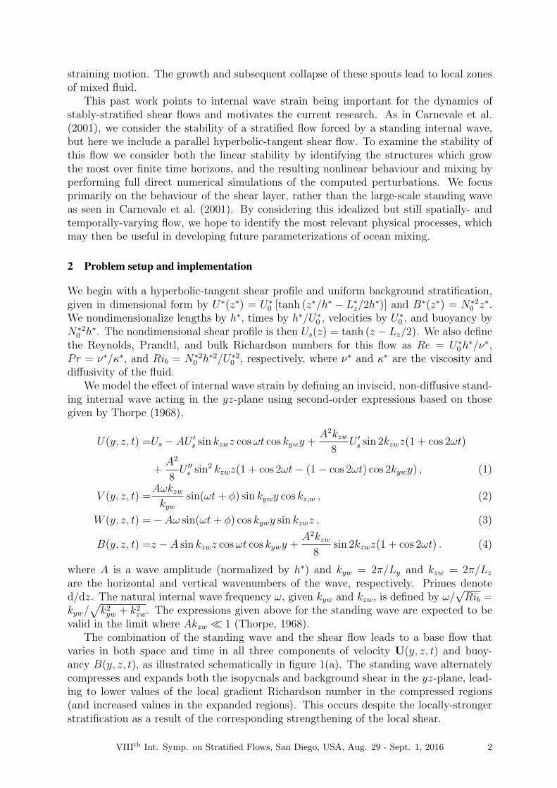
varies in both space and time in all three components of velocity U(y, z, t) and buoy-ancy B(y, z, t), as illustrated schematically in figure 1(a). The standing wave alternatelycompresses and expands both the isopycnals and background shear in the yz-plane, lead-ing to lower values of the local gradient Richardson number in the compressed regions(and increased values in the expanded regions). This occurs despite the locally-strongerstratification as a result of the corresponding strengthening of the local shear.

VIIIth Int. Symp. on Stratified Flows, San Diego, USA, Aug. 29 - Sept. 1, 2016 2

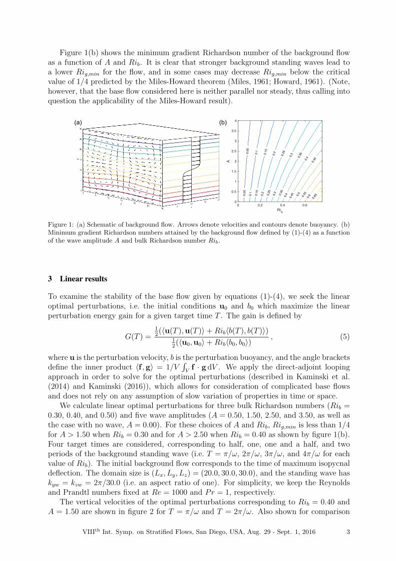
Figure 1(b) shows the minimum gradient Richardson number of the background flowas a function of A and Rib. It is clear that stronger background standing waves lead toa lower Rig,min for the flow, and in some cases may decrease Rig,min below the criticalvalue of 1/4 predicted by the Miles-Howard theorem (Miles, 1961; Howard, 1961). (Note,however, that the base flow considered here is neither parallel nor steady, thus calling intoquestion the applicability of the Miles-Howard result).

(a)

0 0.2 0.4 0.6Rib

0

0.5

1

1.5

2

2.5

3

3.5

4

A

0.05

0.05

0.1

0.1

0.15

0.15

0.2

0.2

0.25

0.25

0.3

0.3

0.35

0.35

0.4

0.4

0.45

0.45 0.5

0.55

0.6 0.65

(b)

Figure 1: (a) Schematic of background flow. Arrows denote velocities and contours denote buoyancy. (b)Minimum gradient Richardson numbers attained by the background flow defined by (1)-(4) as a functionof the wave amplitude A and bulk Richardson number Rib.

3 Linear results

To examine the stability of the base flow given by equations (1)-(4), we seek the linearoptimal perturbations, i.e. the initial conditions u0 and b0 which maximize the linearperturbation energy gain for a given target time T . The gain is defined by

G(T ) =12(〈u(T ),u(T )〉+Rib〈b(T ), b(T )〉)

12(〈u0,u0〉+Rib〈b0, b0〉)

, (5)

where u is the perturbation velocity, b is the perturbation buoyancy, and the angle bracketsdefine the inner product 〈f ,g〉 = 1/V

∫Vf · g dV . We apply the direct-adjoint looping

approach in order to solve for the optimal perturbations (described in Kaminski et al.(2014) and Kaminski (2016)), which allows for consideration of complicated base flowsand does not rely on any assumption of slow variation of properties in time or space.

We calculate linear optimal perturbations for three bulk Richardson numbers (Rib =0.30, 0.40, and 0.50) and five wave amplitudes (A = 0.50, 1.50, 2.50, and 3.50, as well asthe case with no wave, A = 0.00). For these choices of A and Rib, Rig,min is less than 1/4for A > 1.50 when Rib = 0.30 and for A > 2.50 when Rib = 0.40 as shown by figure 1(b).Four target times are considered, corresponding to half, one, one and a half, and twoperiods of the background standing wave (i.e. T = π/ω, 2π/ω, 3π/ω, and 4π/ω for eachvalue of Rib). The initial background flow corresponds to the time of maximum isopycnaldeflection. The domain size is (Lx, Ly, Lz) = (20.0, 30.0, 30.0), and the standing wave haskyw = kzw = 2π/30.0 (i.e. an aspect ratio of one). For simplicity, we keep the Reynoldsand Prandtl numbers fixed at Re = 1000 and Pr = 1, respectively.

The vertical velocities of the optimal perturbations corresponding to Rib = 0.40 andA = 1.50 are shown in figure 2 for T = π/ω and T = 2π/ω. Also shown for comparison

VIIIth Int. Symp. on Stratified Flows, San Diego, USA, Aug. 29 - Sept. 1, 2016 3

is the optimal perturbation for the same target times with A = 0.00. The primaryeffect of the standing wave on the structure of the optimal perturbation is to localize itin the y-direction in regions of high vertical strain rate, as shown by figures 2(b) and(d). In particular, the perturbations localize such that they benefit from the effectsof vertical compressive strain during their evolution, as discussed below. Within thelocalized region, the structure of the optimal perturbations in the xz-plane is similar tothat of the perturbations for the shear layer alone, namely a series of rolls tilted againstthe background shear flow as required for energy growth via the Orr mechanism (Orr,1907).

(a) (d)(b) (c)

xyz

Figure 2: Structure of computed linear optimal perturbations for short target times. The colours denotethe perturbation vertical velocities, and the isosurfaces show the background buoyancy field. (a) A = 0.00and T = π/ω. (b) A = 1.50 and T = π/ω. (c) A = 0.00 and T = 2π/ω. (d) A = 1.50 and T = 2π/ω.Rib = 0.40 for all cases shown here.

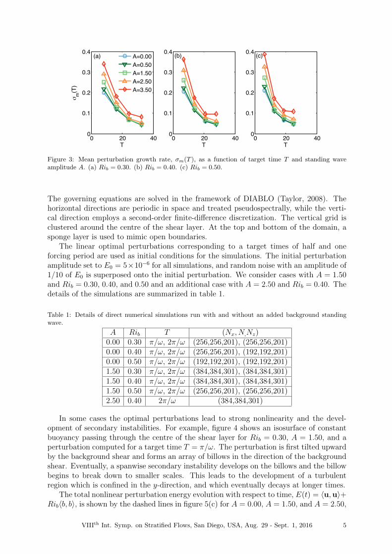
Figure 3 shows the computed optimal mean growth rate σm(T ) = lnG(T )/2T . Theperturbation energy growth may be substantially increased in the presence of standingwaves compared to the unstrained case (A = 0.00). At longer times, the mean growthrates plateau as the normal-mode instability associated with the standing wave dominates(Bouruet-Aubertot et al., 1995), but much higher mean growth rates σm(T ) are found atshorter times. This is in agreement with the observation in Kaminski et al. (2014) whereperturbations to base flows that allowed for Kelvin-Helmholtz instability still attainedhigher growth rates than the predicted normal-mode growth rates at shorter T . It isworth noting that the O(0.1) growth rates are of the same order as the background forcingfrequency (where ω ∼ 0.4 − 0.5), indicating that the perturbations evolve on a similartimescale to the variation of the background flow. Thus, the frozen-in-time approachcommonly used in linear stability analysis would not have been justified here.

By examining the details of the perturbation energy budget (not presented here), it canbe shown that the enhanced linear perturbation energy gain arises due to an enhancementof the existing shear-based transient growth mechanism for unstrained flows (Kaminskiet al., 2014). That is, the vertical internal wave strain acts to catalyze perturbationgrowth via shear.

4 Nonlinear results

Given the significant linear perturbation energy gain, it is natural to ask whether theoptimal perturbations computed in the previous section would be susceptible to non-linear effects. To examine this question, we carry out direct numerical simulations bysolving the full Boussinesq Navier-Stokes and buoyancy conservation equations govern-ing the evolution of perturbations u and b for a prescribed background flow U and B.

VIIIth Int. Symp. on Stratified Flows, San Diego, USA, Aug. 29 - Sept. 1, 2016 4

0 20 400

0.1

0.2

0.3

0.4

T

σm

(T)

0 20 400

0.1

0.2

0.3

0.4

T0 20 400

0.1

0.2

0.3

0.4

T

A=0.00A=0.50A=1.50A=2.50A=3.50

(a) (b) (c)

Figure 3: Mean perturbation growth rate, σm(T ), as a function of target time T and standing waveamplitude A. (a) Rib = 0.30. (b) Rib = 0.40. (c) Rib = 0.50.

The governing equations are solved in the framework of DIABLO (Taylor, 2008). Thehorizontal directions are periodic in space and treated pseudospectrally, while the verti-cal direction employs a second-order finite-difference discretization. The vertical grid isclustered around the centre of the shear layer. At the top and bottom of the domain, asponge layer is used to mimic open boundaries.

The linear optimal perturbations corresponding to a target times of half and oneforcing period are used as initial conditions for the simulations. The initial perturbationamplitude set to E0 = 5×10−6 for all simulations, and random noise with an amplitude of1/10 of E0 is superposed onto the initial perturbation. We consider cases with A = 1.50and Rib = 0.30, 0.40, and 0.50 and an additional case with A = 2.50 and Rib = 0.40. Thedetails of the simulations are summarized in table 1.

Table 1: Details of direct numerical simulations run with and without an added background standingwave.

A Rib T (Nx, N,Nz)0.00 0.30 π/ω, 2π/ω (256,256,201), (256,256,201)0.00 0.40 π/ω, 2π/ω (256,256,201), (192,192,201)0.00 0.50 π/ω, 2π/ω (192,192,201), (192,192,201)1.50 0.30 π/ω, 2π/ω (384,384,301), (384,384,301)1.50 0.40 π/ω, 2π/ω (384,384,301), (384,384,301)1.50 0.50 π/ω, 2π/ω (256,256,201), (256,256,201)2.50 0.40 2π/ω (384,384,301)

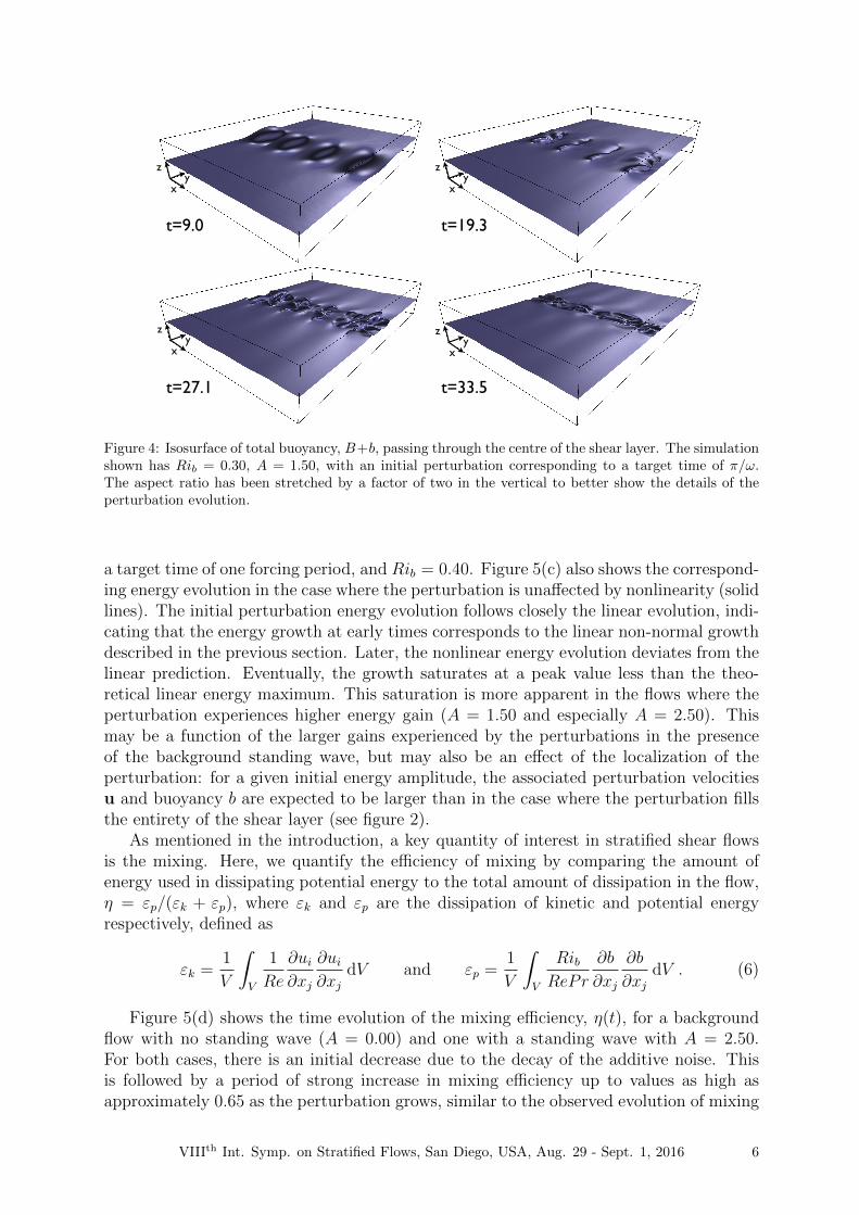
In some cases the optimal perturbations lead to strong nonlinearity and the devel-opment of secondary instabilities. For example, figure 4 shows an isosurface of constantbuoyancy passing through the centre of the shear layer for Rib = 0.30, A = 1.50, and aperturbation computed for a target time T = π/ω. The perturbation is first tilted upwardby the background shear and forms an array of billows in the direction of the backgroundshear. Eventually, a spanwise secondary instability develops on the billows and the billowbegins to break down to smaller scales. This leads to the development of a turbulentregion which is confined in the y-direction, and which eventually decays at longer times.

The total nonlinear perturbation energy evolution with respect to time, E(t) = 〈u,u〉+Rib〈b, b〉, is shown by the dashed lines in figure 5(c) for A = 0.00, A = 1.50, and A = 2.50,

VIIIth Int. Symp. on Stratified Flows, San Diego, USA, Aug. 29 - Sept. 1, 2016 5

x

zy

x

zy

t=19.3

t=33.5

x

zy

x

zy

t=9.0

t=27.1

Figure 4: Isosurface of total buoyancy, B+b, passing through the centre of the shear layer. The simulationshown has Rib = 0.30, A = 1.50, with an initial perturbation corresponding to a target time of π/ω.The aspect ratio has been stretched by a factor of two in the vertical to better show the details of theperturbation evolution.

a target time of one forcing period, and Rib = 0.40. Figure 5(c) also shows the correspond-ing energy evolution in the case where the perturbation is unaffected by nonlinearity (solidlines). The initial perturbation energy evolution follows closely the linear evolution, indi-cating that the energy growth at early times corresponds to the linear non-normal growthdescribed in the previous section. Later, the nonlinear energy evolution deviates from thelinear prediction. Eventually, the growth saturates at a peak value less than the theo-retical linear energy maximum. This saturation is more apparent in the flows where theperturbation experiences higher energy gain (A = 1.50 and especially A = 2.50). Thismay be a function of the larger gains experienced by the perturbations in the presenceof the background standing wave, but may also be an effect of the localization of theperturbation: for a given initial energy amplitude, the associated perturbation velocitiesu and buoyancy b are expected to be larger than in the case where the perturbation fillsthe entirety of the shear layer (see figure 2).

As mentioned in the introduction, a key quantity of interest in stratified shear flowsis the mixing. Here, we quantify the efficiency of mixing by comparing the amount ofenergy used in dissipating potential energy to the total amount of dissipation in the flow,η = εp/(εk + εp), where εk and εp are the dissipation of kinetic and potential energyrespectively, defined as

εk =1

V

∫V

1

Re

∂ui∂xj

∂ui∂xj

dV and εp =1

V

∫V

RibRePr

∂b

∂xj

∂b

∂xjdV . (6)

Figure 5(d) shows the time evolution of the mixing efficiency, η(t), for a backgroundflow with no standing wave (A = 0.00) and one with a standing wave with A = 2.50.For both cases, there is an initial decrease due to the decay of the additive noise. Thisis followed by a period of strong increase in mixing efficiency up to values as high asapproximately 0.65 as the perturbation grows, similar to the observed evolution of mixing

VIIIth Int. Symp. on Stratified Flows, San Diego, USA, Aug. 29 - Sept. 1, 2016 6

0 10 20 300

2

4

x 10−4

t

E(t)

A=0.00, linearA=0.00, nonlinA=1.50, linearA=1.50, nonlinA=2.50, linearA=2.50, nonlin

0 10 20 30 40 50−0.5

0

0.5

dW/d

z

0 10 20 30−0.5

0

0.5

dW/d

z

0 10 20 30 40 500

0.2

0.4

0.6

0.8

t

η(t)

A=0.00A=2.50

(a) (b)

(d)(c)

Figure 5: (a),(c) Background vertical strain rate, ∂W/∂z, through the centre of the perturbation (y =Ly/2, z = Lz/2). (b) Time evolution of total perturbation energy E(t) for linear (solid) and nonlinear(dashed) simulations. The blue lines correspond to A = 0.00, the red lines to A = 1.50, and the greenlines to A = 2.50. (d) Time evolution of mixing efficiency, η(t), for A = 0.00 and A = 2.50. The casesshown have Rib = 0.40 and T = 2π/ω.

efficiency for Kelvin-Helmholtz instability (Peltier and Caulfield, 2003). As the perturba-tions continue to evolve, the mixing efficiency decreases to a value of approximately 0.3.However, the influence of the background flow is apparent, with increasing mixing effi-ciency during times of compressive vertical strain rate (∂W/∂z < 0). This is in contrastto the unstrained flow for which the mixing efficiency is tending towards a constant valueafter the initial transient evolution.

5 Conclusions

Here we have computed the linear optimal perturbations corresponding to a base flowconsisting of a parallel, steady stratified shear flow interacting with a large-scale standinginternal wave, based on the expressions given by Thorpe (1968). The straining flowassociated with the internal wave acts to alternately compress and expand the shearlayer, modifying the shear and stratification in space and in time.

Over time horizons of the order of one wave period, the added standing wave in-creases the maximum perturbation energy gain by up to an order of magnitude, withhigher increases observed for larger-amplitude waves. In contrast to the optimal pertur-bations computed for the stratified shear layer alone, the perturbations to the strainedflow localize in regions of high-amplitude vertical strain rate, ∂W/∂z. In the presenceof compressive strain (∂W/∂z < 0), the growth of perturbation energy via vertical shearproduction is enhanced, leading to higher perturbation energy growth via the shear-basedOrr mechanism. At longer target times, there is a shift in the growth mechanism favouredby the optimal perturbations to the normal-mode instability of the standing wave.

We have also performed complementary direct numerical simulations, initialized bygiving the computed optimal perturbations a small but finite initial amplitude. Theperturbations grow linearly before saturating at larger amplitudes. The energy growthis sufficient to cause strongly nonlinear effects such as the development of billows, andfor certain parameters the flow transitions to turbulence. Mixing efficiencies vary in time

VIIIth Int. Symp. on Stratified Flows, San Diego, USA, Aug. 29 - Sept. 1, 2016 7

with the background straining flow, suggesting that the phase of the turbulent event isan additional factor in determining the associated mixing efficiency.

ReferencesAlford, M. H. and Pinkel, R. (2000). Observations of overturning in the thermocline: the

context of ocean mixing. J. Phys. Oceanogr., 30:805–832.

Aucan, J., Merrifield, M. A., Luther, D. S., and Flament, P. (2006). Tidal mixing eventson the deep flanks of Kaena Ridge, Hawaii. J. Phys. Oceanogr., 36:1202–1219.

Bouruet-Aubertot, P., Sommeria, J., and Staquet, C. (1995). Breaking of standing internalgravity waves through two-dimensional instabilities. J. Fluid Mech., 285:265–301.

Carnevale, G. F., Briscolini, M., and Orlandi, P. (2001). Buoyancy- to inertial-rangetransition in forced stratified turbulence. J. Fluid Mech., 427:205–239.

Farrell, B. F. and Ioannou, P. J. (1993). Transient development of perturbations instratified shear flow. J. Atmos. Sci., 50(14):2201–2214.

Howard, L. N. (1961). Note on a paper of John W. Miles. J. Fluid Mech., 10:509–512.

Kaminski, A. K. (2016). Linear optimal perturbations and transition to turbulence instrongly stratified shear flows. PhD thesis, University of Cambridge.

Kaminski, A. K., Caulfield, C. P., and Taylor, J. R. (2014). Transient growth in stronglystratified shear layers. J. Fluid Mech., 758:R4.

Levine, M. D. and Boyd, T. J. (2006). Tidally forced internal waves and overturns observedon a slope: results from HOME. J. Phys. Oceanogr., 36:1184–1201.

Mellor, G. L. and Yamada, T. (1982). Development of a turbulence closure model forgeophysical fluid problems. Rev. Geophys. Space Phys., 20(4):851–875.

Miles, J. W. (1961). On the stability of heterogeneous shear flows. J. Fluid Mech.,496:496–508.

Orr, W. M. (1907). The stability or instability of the steady motions of a perfect liquidand of a viscous liquid. Part I: A perfect liquid. Proc. R. Irish Acad. A, 27:9–68.

Peltier, W. R. and Caulfield, C. P. (2003). Mixing efficiency in stratified shear flows.Annu. Rev. Fluid Mech., 35:135–167.

Price, J. F., Weller, R. A., and Pinkel, R. (1986). Diurnal cycling: Observations andmodels of the upper ocean response to diurnal heating, cooling, and wind mixing. J.Geophys. Res., 91(C7):8411–8427.

Taylor, J. R. (2008). Numerical simulations of the stratified oceanic bottom boundarylayer. PhD thesis, University of California, San Diego.

Thorpe, S. A. (1968). On standing internal gravity waves of finite amplitude. J. FluidMech., 32(3):489–528.

VIIIth Int. Symp. on Stratified Flows, San Diego, USA, Aug. 29 - Sept. 1, 2016 8