Turbulent mixing in a strongly forced salt wedge estuary · Turbulent mixing in a strongly forced...

Turbulent mixing in a strongly forced salt wedge estuary

David K. Ralston,1 W. Rockwell Geyer,1 James A. Lerczak,2 and Malcolm Scully3

Received 18 December 2009; revised 9 August 2010; accepted 8 September 2010; published 9 December 2010.

[1] Turbulent mixing of salt is examined in a shallow salt wedge estuary with strongfluvial and tidal forcing. A numerical model of the Merrimack River estuary is used toquantify turbulent stress, shear production, and buoyancy flux. Little mixing occurs duringflood tides despite strong velocities because bottom boundary layer turbulence isdislocated from stratification elevated in the water column. During ebbs, bottom salinityfronts form at a series of bathymetric transitions. At the fronts, near‐bottom velocity andshear stress are low, but shear, stress, and buoyancy flux are elevated at the pycnocline.Internal shear layers provide the dominant source of mixing during the early ebb. Later inthe ebb, the pycnocline broadens and moves down such that boundary layer turbulencedominates mixing. Mixing occurs primarily during ebbs, with internal shear mixingaccounting for about 50% of the total buoyancy flux. Both the relative contribution ofinternal shear mixing and the mixing efficiency increase with discharge, with bulk mixingefficiencies between 0.02 and 0.07. Buoyancy fluxes in the estuary increase with dischargeup to about 400 m3 s−1 above which a majority of the mixing occurs offshore. Observedbuoyancy fluxes were more consistent with the k‐" turbulence closure than theMellor‐Yamada closure, and more total mixing occurred in the estuary with k‐".Calculated buoyancy fluxes were sensitive to horizontal grid resolution, as a lowerresolution grid yielded less integrated buoyancy flux in the estuary and exported lowersalinity water but likely had greater numerical mixing.

Citation: Ralston, D. K., W. R. Geyer, J. A. Lerczak, and M. Scully (2010), Turbulent mixing in a strongly forced salt wedgeestuary, J. Geophys. Res., 115, C12024, doi:10.1029/2009JC006061.

1. Introduction

[2] Turbulent mixing of salt and freshwater in estuariesaffects the stratification, the length of the salinity intrusion,and the exchange of biological or chemical constituentsbetween the river and coastal ocean. Where, when, and howthat mixing occurs depends on the estuarine forcing. Pre-vious work has examined turbulence and mixing in partiallystratified estuaries like the Hudson River [Peters, 1999;Trowbridge et al., 1999; Chant et al., 2007] and San Fran-cisco Bay [Stacey et al., 1999]. Observations in partiallymixed estuaries have found that bottom boundary layershear is the dominant source of turbulence [Trowbridge etal., 1999] and that salinity mixing occurs primarily due tobottom boundary layer turbulence during flood tides [Peters,1999; MacCready and Geyer, 2001; Chant et al., 2007].Turbulence is generated at the bed and decreases in energywith distance above the bed due to overlying stratification,

particularly during ebbs when tidal straining helps tomaintain stratification [Stacey et al., 1999].[3] In contrast, observations in strongly stratified estuaries

have noted the importance of interfacial shear instabilitiesfor mixing [Partch and Smith, 1978; Geyer and Farmer,1989; Uncles and Stephens, 1996; Jay and Smith, 1990a;Kay and Jay, 2003; MacDonald and Horner‐Devine, 2008].Strong shear can develop across the pycnocline during ebbsin tidal salt wedge estuaries leading to turbulence andmixing that is maximal midwater column, while bottomboundary layer mixing is relatively weak. The differencesbetween partially and highly stratified estuaries indicatethat the magnitude, mechanisms, and phasing of verticalsalt flux vary through estuarine parameter space. How thesemixing processes depend on estuarine characteristics likeriver discharge, tidal amplitude, and bathymetry remains tobe quantified.[4] The focus here is on turbulent salt flux in an estuary

where river and tidal velocities are significant and steadybaroclinic circulation is comparatively weak. The study siteis the Merrimack River on the northeast coast of the UnitedStates, but conditions in the Merrimack are representative oftime‐dependent salt wedge estuaries like the Columbia [Jayand Smith, 1990b], Connecticut [Garvine, 1975], Fraser[Geyer and Farmer, 1989], and Snohomish River [Wanget al., 2009] estuaries. These estuaries are short (the lengthof the salinity intrusion is similar to the tidal excursion),

1Applied Ocean Physics and Engineering, Woods Hole OceanographicInstitution, Woods Hole, Massachusetts, USA.

2College of Oceanic andAtmospheric Sciences, Oregon State University,Corvallis, Oregon, USA.

3Department of Ocean, Earth, and Atmospheric Sciences, OldDominion University, Norfolk, Virginia, USA.

Copyright 2010 by the American Geophysical Union.0148‐0227/10/2009JC006061

JOURNAL OF GEOPHYSICAL RESEARCH, VOL. 115, C12024, doi:10.1029/2009JC006061, 2010

C12024 1 of 19

http://dx.doi.org/10.1029/2009JC006061

strongly stratified, and have strong along‐estuary salinitygradients. Recent work in the Merrimack has described thestructure and variability of the salinity and velocity fields andlongitudinal salt flux mechanisms [Ralston et al., 2010].[5] The goal here is to characterize and quantify turbulent

mixing in a tidal salt wedge estuary, including how muchmixing occurs, when mixing happens during the tidal cycle,where mixing occurs in the estuary, and what turbulencegeneration mechanisms are responsible. Turbulence andmixing are notoriously difficult to quantify in the field, soour approach is to use a numerical model that has beenvalidated against extensive observations of salinity andvelocity. Turbulence and mixing are calculated in the modeland are evaluated over a range of forcing conditions,including seasonal variability in river discharge and spring‐neap variability in tidal amplitude. Mixing mechanisms areexpected to vary with forcing and to affect the location andefficiency of turbulent salt flux. We evaluate the model re-sults by comparison with observations of turbulence in theMerrimack and consider the sensitivity of the results toturbulence closure and grid resolution.

2. Methods

2.1. Site Description

[6] The Merrimack River flows into the Gulf of Mainewith a mean annual discharge of 220 m3 s−1. Seasonally, thedischarge ranges from about 1500 m3 s−1 during the springfreshet to less than 50 m3 s−1 in late summer. The lower 35km of the river are tidal, with a mean tidal range at themouth of 2.5 m and a spring tidal range of about 4 m. In theupper estuary, the channel is narrow with a series of sills(typical depth of 4–6 m) and deeper holes (typical depth of8–10 m) (Figure 1). Between 1.5 and 5 km from the mouththe estuary broadens into an embayment with intertidal flatsand fringing salt marsh. The channel at the mouth passesbetween barrier islands and is constrained by rock jetties. Ashallow ebb tide bar (4 m deep) is located about 0.5 kmoffshore of the mouth.

2.2. Observations

[7] Observations from moored instruments and shipboardsurveys in the Merrimack during the spring and summer of2005 were used to develop and calibrate the numerical model[Ralston et al., 2010] Along‐channel and across‐channelmooring arrays measured surface elevation, velocity profiles,and surface and bottom salinities. Tidal cycle surveys wereconducted to record the along‐channel salinity distributionand the lateral salinity and velocity distributions at crosssections in the estuary. Hydrographic surveys correspondedwith river discharges of 250, 550, and 350 m3 s−1.[8] Additional observations were made in May 2007

using the Measurement Array for Sensing Turbulence(MAST) [Geyer et al., 2008]. The MAST is a 10 m longspar with instrument brackets at multiple elevations tomeasure turbulent fluctuations in velocity and salinity. Eachbracket holds an acoustic Doppler velocimter (ADV, sam-pling at 25 Hz) and a fast response conductivity sensor(sampling at 200 Hz) with sampling volumes offset by 2 cmin the flow direction. Salinity dominates the conductivitysignal, so the colocated measurements at turbulent timescales allow direct covariance estimates of vertical salt flux

s0w0 . Additional instruments on the MAST include con-ductivity‐temperature (CT) and pressure sensors. TheMAST is attached to a research vessel and provides con-tinuous time series of turbulent mixing at multiple eleva-tions spanning most of the estuarine water column.[9] The MAST was used in the Merrimack in May 2007

over 3 days with moderate river discharge (350 m3 s−1) andtidal amplitude (2.6 m range). The MAST was deployedfrom an anchored research vessel in 6–8 m water depth(location shown in Figure 1). A second research vesselconducted simultaneous along‐ and across‐channel surveysof salinity and velocity in the vicinity of the anchor site.Details on the MAST data processing can be found in thework of Geyer et al. [2008].

2.3. Numerical Model

[10] We have developed a numerical model of the Mer-rimack using the Finite Volume Coastal Ocean Model [Chenet al., 2003, 2008]. FVCOM uses an unstructured horizontalgrid of triangles and sigma layers vertically (Figure 1), andthe finite volume approach is locally and globally conser-vative for momentum and scalars. The advection scheme issecond‐order accurate, and in test domains the accuracycompared well with higher‐order advection schemes in astructured grid model [Huang et al., 2008]. Horizontal gridresolution varied from about 20 m in the estuarine channelto about 3000 m near the offshore boundary; note that theoffshore open boundaries are approximately 35 km from theriver mouth (not shown in Figure 1). FVCOM includeswetting and drying, with cells becoming inactive whenwater level is less than 0.05 m. Twenty sigma levels wereused vertically. Ten vertical levels provided insufficientresolution of the vertical structure of salinity and velocity,but simulations with 30 levels were quantitatively similar to20 level cases. Note that temperature is not modeled becausesalinity dominates the density variations.[11] The bathymetry for the model grid was based on

NOAA soundings and was refined with additional bathy-metric data collected in 2005 and 2007. Boundary condi-tions included tidal forcing offshore and river flowupstream. For the observation periods, the tidal record fromthe National Oceanic and Atmospheric Administration(NOAA) station at Boston (#8443970) was used as theboundary water surface elevation. River discharge data fromthe U.S. Geological Survey (USGS) gage at Lowell(#01100000) was multiplied by 1.1 to account for inputsbelow the gauging station. The depth‐dependent, time‐varying salinity at the offshore boundary was based on datafrom Gulf of Maine Ocean Observing System buoys inMassachusetts Bay (Buoy A) and on the Western MaineShelf (Buoy B).[12] FVCOM incorporates turbulence closure schemes

through the General Ocean Turbulence Model (GOTM).GOTM is a 1‐D vertical module that recasts various closureschemes in a uniform format [Umlauf and Burchard, 2003].For the model to reproduce the strong pycnocline observedduring high discharge conditions, it was important to set thebackground turbulent diffusivity to a small value (10−7 m2 s−1

in these simulations, but results were similar for 10−6 m2 s−1).Similarly, the subgrid scale horizontal diffusivity was set tozero to limit mixing of the sharp horizontal salinity gradients.Several turbulence closure schemes were tested. Most of the

RALSTON ET AL.: MIXING IN A SALT WEDGE ESTUARY C12024C12024

2 of 19

results presented use the k‐" closure [Rodi, 1987] with sta-bility coefficients from Canuto et al. [2001, version “A”], butwe also consider k‐" with stability coefficients from Kanthaand Clayson [1994] and the Mellor‐Yamada level 2.5 closure[Mellor and Yamada, 1982].[13] The model was calibrated by adjusting the bottom

roughness (z0) to match the tidal advection of the salinityintrusion from moored instruments in 2005. The sameconstant, uniform value of z0 = 0.5 cm was used for simu-lations of the May 2007 observation period. The model re-sults compared favorably with surveyed along‐ and across‐channel distributions of salinity and velocity [see Ralston etal., 2010, for details]. In addition to the realistic forcing,

idealized simulations were run over the expected range oftidal and fluvial forcing for the Merrimack. Dischargeranged over seasonal low to high flows (25, 50, 100, 200,400, 700, 1000, and 2000 m3 s−1) and tides ranged fromneap to spring amplitudes (2.0, 2.4, 2.8, and 3.2 m range).[14] We consider when mixing occurs through the tidal

cycle (flood‐ebb asymmetry), where mixing occurs in theestuary (localized or distributed), what the dominant me-chanisms for mixing are (bottom boundary layer or freeshear layer turbulence), and how the mixing depends onforcing (spring‐neap tides and river discharge). We use themodel to calculate directly the mixing of momentum andsalt. For momentum transfer in the water column, the

Figure 1. (top) Bathymetry for the Merrimack River estuary, including location of the MAST ebbanchor station measurements in 2007. (bottom) FVCOM model grid, indicating distance (km) from themouth in the along‐channel transects shown in Figures 2 and 3. Note this plot focuses on the estuaryand that the full grid extends offshore from the mouth approximately 35 km to the north, east, and south,and up‐river 25 km to the west.


3 of 19

magnitude of the shear stress is expressed as ktk = k(u0w′,v0w′)k = Km[(∂u/∂z)2 + (∂v/∂z)2]1/2, where Km is the eddyviscosity from the turbulence closure. The stress (or frictionvelocity) at the bed is u*

2 = Cdu12 where Cd is the drag

coefficient and u1 is the velocity at the lowest sigma level atdistance z1 from the bed. The drag coefficient depends on

the bed roughness (z0): Cd = �=lnz1 þ z0

z0

� �� 2. As in the

model, this assumes a log layer velocity profile immedi-ately above the bed. The buoyancy flux that mixes saltvertically is B =

g

�0�0w0 = −gbKh∂s/∂z where Kh is the

eddy diffusivity and b is the coefficient of saline con-traction (b = 7.7 × 10−4 psu−1, with r = r0(1 + bs). Weuse buoyancy flux as a measure of the turbulent mixing ofsalt, but an alternative approach would be to calculate the

decay in depth‐integrated salinity variance [Burchard etal., 2009]. The buoyancy flux is derived directly fromthe turbulence closure (Kh) and stratification, but the cal-culated mixing would be reduced by instances of con-vective mixing when B < 0. Generally the two approachesgive similar results [Burchard et al., 2009], but thetreatment of convective instabilities in turbulence model-ing remains an area of research and the use of scalarvariance decay to assess mixing avoids this issue.

3. Results

3.1. Estuarine Buoyancy Flux

[15] For a section along the channel (location shown inFigure 1), we plot the shear stress and buoyancy flux atinstances through the flood (Figure 2) and ebb (Figure 3)

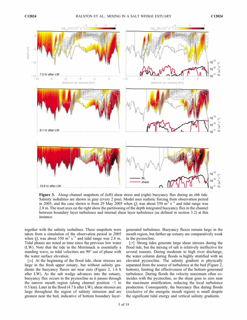
Figure 2. Along‐channel snapshots of (left) shear stress and (right) instantaneous buoyancy flux duringa flood tide. (Log scale, so B < 0 not shown). Salinity isohalines are shown in gray (every 2 psu). Modeluses realistic forcing from observation period in 2005, and the case shown is from 29 May 2005 when Qr

was about 550 m3 s−1 and tidal range was 2.8 m. The inset axes on the right show the partitioning of thedepth integrated buoyancy flux in the channel between boundary layer turbulence and internal shear layerturbulence (as defined in section 3.2) at this instance.


4 of 19

together with the salinity isohalines. These snapshots weretaken from a simulation of the observation period in 2005when Qr was about 550 m3 s−1 and tidal range was 2.8 m.Tidal phases are noted as time since the previous low water(LW). Note that the tide in the Merrimack is essentially astanding wave, so tidal velocities are 90° out of phase withthe water surface elevation.[16] At the beginning of the flood tide, shear stresses are

large in the fresh upper estuary, but without salinity gra-dients the buoyancy fluxes are near zero (Figure 2, 1.6 hafter LW). As the salt wedge advances into the estuary,buoyancy flux occurs in the pycnocline as it passes throughthe narrow mouth region (along channel position −1 to0.5 km). Later in the flood (4.7 h after LW), shear stresses arelarge throughout the region of salinity intrusion and aregreatest near the bed, indicative of bottom boundary layer‐

generated turbulence. Buoyancy fluxes remain large in themouth region, but farther up‐estuary are comparatively weakin the pycnocline.[17] Strong tides generate large shear stresses during the

flood tide, but the mixing of salt is relatively ineffective forseveral reasons. During moderate to high river discharge,the water column during floods is highly stratified with anelevated pycnocline. The salinity gradient is physicallyseparated from the source of turbulence at the bed (Figure 2,bottom), limiting the effectiveness of the bottom‐generatedturbulence. During floods the velocity maximum often co-incides with the pycnocline, so the shear goes to zero nearthe maximum stratification, reducing the local turbulenceproduction. Consequently, the buoyancy flux during floods(exclusive of the energetic mouth region) is small despitethe significant tidal energy and vertical salinity gradients.

Figure 3. Along‐channel snapshots of (left) shear stress and (right) buoyancy flux during an ebb tide.Salinity isohalines are shown in gray (every 2 psu). Model uses realistic forcing from observation periodin 2005, and the case shown is from 29 May 2005 when Qr was about 550 m3 s−1 and tidal range was2.8 m. The inset axes on the right show the partitioning of the depth integrated buoyancy flux in the channelbetween boundary layer turbulence and internal shear layer turbulence (as defined in section 3.2) at thisinstance.


5 of 19

[18] During the early ebb (Figure 3, 7.5 h after LW),boundary‐generated stresses occur in regions of weak strati-fication up‐estuary, but several patches of elevated stressare also located in the pycnocline (along‐channel position−7.5 km, −6.9 km, and −4.3 km). These regions of enhancedshear stress and mixing correspond with bathymetric sillsand expansions. The mixing occurs mid water column andis distinct from bottom boundary layer turbulence. Later inthe ebb, the stress and buoyancy flux at these locationsbecomes directly associated with bottom‐generated turbu-lence (e.g., −4.3 km at 9.1 h after LW). As for the flood,the energetic mouth region has high stresses and buoyancyfluxes, particularly late ebb. As velocities intensify and thesalt wedge breaks down (10.6 h after LW), the buoyancyfluxes increase and become more uniform along the chan-nel from midestuary out the bar. Overall, the buoyancy fluxin the estuary during the ebb is significantly greater thanduring the flood.[19] The map of depth‐integrated, tidally averaged buoy-

ancy flux (hB̂i, with angle brackets for tidally averagedquantities and a hat for depth averaged) for the same tidalcycle illustrates the strong mixing in the mouth region butalso shows lateral heterogeneity not apparent in the along‐channel sections (Figure 4). Rock jetties at the mouth con-strain the flow and create high velocities. Strong turbulenceand secondary circulation due to the channel curvatureinduce mixing during both flood and ebb. Farther up‐estuarythe geometry is not as abrupt and constrained as at the mouth,and localized regions of intensified mixing are at the sills(−7.5 km and −6.9 km) and the sill and expansion onto thetidal flats (−4.3 km). The total mixing energy at thesebathymetric transitions is less than at the mouth and bar, but itis substantial relative to the mixing at other locations in theestuarine interior.[20] Outside the estuary, hB̂i in the plume is patchier. The

patchiness occurs as a result of small temporal and spatialfluctuations in gradient Richardson number that allow orsuppress mixing according to the turbulence closure. Thepatchiness results in part from an undersampling of themodel with output every 15 min rather than at every timestep. A continuous time integration or longer averaging

period would generate a more spatially uniform distributionof mixing in the offshore plume than this discrete samplingover a tidal cycle.

3.2. Mechanisms of Mixing: Internal Shear VersusBoundary Layer Mixing

[21] We now consider two different mixing mechanisms,one in which the mixing originates as instability of a shearlayer and the other in which the turbulence is generated atthe bottom boundary. Shear layer turbulence is most dis-tinctive during the early to midebb when weak near‐bottomcurrents and the baroclinic gradient (often associated withtopographic transitions at sills and expansions) enhanceshear across the pycnocline and lead to shear instabilities[Geyer and Smith, 1987]. Boundary induced mixing is thedominant mechanism in partially stratified estuaries [Peters,1999], but it is also important in the highly stratified Mer-rimack. Boundary mixing is most effective when near‐bottom currents are strong and the boundary layer is stratified.[22] In the boundary layer, the maximum shear stress is

near the bed and decreases with distance from the bed. Forinternal shear, the maximum stress occurs in the middle ofthe shear layer. At times, local maxima in shear stress existsimultaneously near the bed and in the upper water column.To quantify the relative contributions of boundary layer andshear layer mixing to the total buoyancy flux, we evaluateshear stress profiles in each grid cell at each output timestep. Locations where shear stress decreases monotonicallywith distance above the bed are assigned entirely toboundary layer turbulence. Locations with a local minimumin stress middepth are divided between the processes, withmixing below the elevation of minimum stress attributed toboundary layer turbulence and above the stress minimumassigned to internal shear. This simulation (as well as theparametric studies described later) was for a period withnegligible wind forcing, but to extend this approach torealistic simulations with wind stress would require similarseparation between the surface boundary layer and internalshear.[23] Using these definitions, the total buoyancy flux inside

the estuary can be divided into boundary layer and shear

Figure 4. Depth‐integrated, tidally averaged buoyancy flux for the period shown in Figures 2 and 3(29 May 2005).


6 of 19

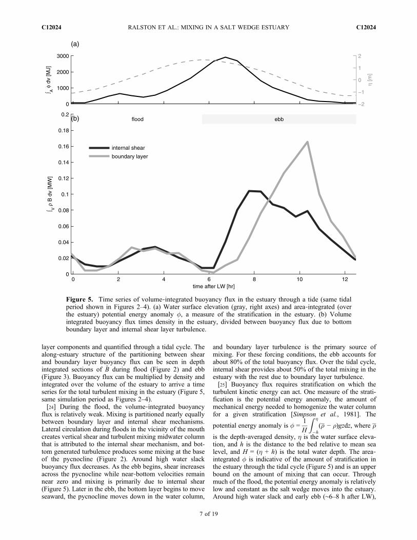
layer components and quantified through a tidal cycle. Thealong‐estuary structure of the partitioning between shearand boundary layer buoyancy flux can be seen in depthintegrated sections of B̂ during flood (Figure 2) and ebb(Figure 3). Buoyancy flux can be multiplied by density andintegrated over the volume of the estuary to arrive a timeseries for the total turbulent mixing in the estuary (Figure 5,same simulation period as Figures 2–4).[24] During the flood, the volume‐integrated buoyancy

flux is relatively weak. Mixing is partitioned nearly equallybetween boundary layer and internal shear mechanisms.Lateral circulation during floods in the vicinity of the mouthcreates vertical shear and turbulent mixing midwater columnthat is attributed to the internal shear mechanism, and bot-tom generated turbulence produces some mixing at the baseof the pycnocline (Figure 2). Around high water slackbuoyancy flux decreases. As the ebb begins, shear increasesacross the pycnocline while near‐bottom velocities remainnear zero and mixing is primarily due to internal shear(Figure 5). Later in the ebb, the bottom layer begins to moveseaward, the pycnocline moves down in the water column,

and boundary layer turbulence is the primary source ofmixing. For these forcing conditions, the ebb accounts forabout 80% of the total buoyancy flux. Over the tidal cycle,internal shear provides about 50% of the total mixing in theestuary with the rest due to boundary layer turbulence.[25] Buoyancy flux requires stratification on which the

turbulent kinetic energy can act. One measure of the strati-fication is the potential energy anomaly, the amount ofmechanical energy needed to homogenize the water columnfor a given stratification [Simpson et al., 1981]. The

potential energy anomaly is � =1

H

Z �

�h(� − r)gzdz, where �

is the depth‐averaged density, h is the water surface eleva-tion, and h is the distance to the bed relative to mean sealevel, and H = (h + h) is the total water depth. The area‐integrated � is indicative of the amount of stratification inthe estuary through the tidal cycle (Figure 5) and is an upperbound on the amount of mixing that can occur. Throughmuch of the flood, the potential energy anomaly is relativelylow and constant as the salt wedge moves into the estuary.Around high water slack and early ebb (∼6–8 h after LW),

Figure 5. Time series of volume‐integrated buoyancy flux in the estuary through a tide (same tidalperiod shown in Figures 2–4). (a) Water surface elevation (gray, right axes) and area‐integrated (overthe estuary) potential energy anomaly �, a measure of the stratification in the estuary. (b) Volumeintegrated buoyancy flux times density in the estuary, divided between buoyancy flux due to bottomboundary layer and internal shear layer turbulence.


7 of 19

the integrated � increases substantially as the bottom layercontinues to move up‐estuary and the surface layer begins toebb, increasing the area with strong stratification. Duringpeak ebb, � in the estuary decreases due to mixing andadvection of stratification to the plume. The � time seriesindicates that the enhanced mixing during ebbs depends inpart on the increase in stratification created by expansion ofthe salt wedge around high water slack.

3.3. Dependence of Buoyancy Flux on Forcing

[26] We expect that the magnitude and mechanisms ofestuarine mixing depend on the relative strengths of tidaland fluvial forcing. To quantify variability in mixingthrough parameter space we ran idealized cases with con-stant discharge and tidal amplitude. Cases included Qr of 25,50, 100, 200, 400, 700, 1000, and 2000 m3 s−1 and tidalrange h0 of 2.0, 2.4, 2.6, and 3.2 m, reflective of the seasonaldischarge and the spring‐neap tidal variability in the Mer-rimack. Each case was run until conditions reached a tidallyperiodic steady state. The tidally averaged horizontal Ri-chardson number (Rix = gb(∂s/∂x)H2/(CdUt

2)) over the rangeof forcing conditions is shown (Figure 6a), but the Merri-mack is highly variable and the temporal and spatial fluc-tuations in Rix are significant, particularly at higher Qr. SeeRalston et al. [2010] a more extensive discussion of how theMerrimack fits into estuarine parameter space.[27] Over the range of discharge and tidal forcing

conditions tested, we find that buoyancy flux in the estuaryis always greater during ebbs than during flood tides(Figure 6b). Here we plot the volume‐integrated buoyancyflux times density integrated over a tidal cycle to yieldmixing energy. The greater mixing during ebbs depends inpart on the stratification and � created around high water(Figure 5). The tidal asymmetry in mixing is most notable atmoderate to high discharge when integrated buoyancy fluxduring the flood is less than half of the mixing during theebb. The mixing during flood tides is not enhanced by riverdischarge, but greater Qr does increase shear and stratifica-tion during ebbs to produce greater total mixing, particularlyat the breakdown of topographic fronts and at the mouth bar.River discharge increases the potential energy anomalyavailable to be mixed (Figure 6c). The tidally averaged,volume integrated � in the estuary increases with Qr exceptfor the highest discharges where the river velocity is suffi-ciently strong to exclude salt water from the estuary for alarge fraction of the tidal cycle. While the total buoyancyinput (and thus potential energy anomaly) is greater forhigher Qr, more mixing is transferred offshore as the lengthof the estuary decreases.[28] For the modeled observation period (Figure 5),

internal shear mixing accounted for about half of the totalbuoyancy flux inside the estuary. Over the broader range ofQr, this ratio varies from about 40% to 65% (Figure 7a,dashed lines). At lower discharges, the estuary becomesmore weakly stratified and fronts are less likely to form attopographic transitions, while at higher discharges the hor-izontal and vertical salinity gradients intensify and the sys-tem becomes more frontal. The mixing mechanisms alsodepended on tidal amplitude; boundary layer mixing ac-counted for a greater proportion of the total buoyancy fluxfor stronger tides. Stronger tidal pressure gradients generate

greater bed stress, thus increasing the relative contributionof the bottom boundary layer.[29] The focus thus far has been on mixing processes

inside the estuary, but freshwater that is not mixed in theestuary enters the plume and eventually mixes with thecoastal ocean. Considering mixing more broadly to includethe region offshore, the relative importance of internal sheargrows substantially and depends more on Qr (Figure 7a,solid lines). At higher discharges, low‐salinity water exitsthe estuary and forms the plume. Most of the mixing in theplume occurs at the base of a thin surface layer separatedfrom the bottom boundary layer by tens of meters of water.Bottom boundary mixing is substantial near the mouthwhere the flow accelerates over the bar and in shallow re-gions along the coast, but farther offshore the bottomstresses do not extend up to the stratification. For moderateto high discharge, internal shear is the primary mixingmechanism away from the bar and accounts for as much as95% of the total mixing in the domain. A relatively smallregion where the plume spreads and decelerates offshore ofthe bar accounts for much of the plume mixing. For highdischarge cases about 75% and for lower discharges about45% of the total offshore mixing occurs within 2 km of themouth.[30] These idealized cases were run with zero wind stress.

In reality, even moderate winds can create a surfaceboundary layer that contributes to mixing the plume. Si-mulations of the observational period that included surfacewind stress had greater mixing in the offshore region thanthose without wind forcing. During periods of weak tomoderate wind (wind speed <4 m s−1), total buoyancy fluxin the offshore region was 1.5–4 times greater than withoutwind. For periods with stronger winds (>4 m s−1), totalbuoyancy flux offshore increased by a factor of 10 to 20over the no‐wind case. Wind mixing of the plume isimportant for plume fate and deserves additional consider-ation, but internal shear instabilities near the lift‐off remaincritical to the creation of the near‐field plume.[31] We quantify the total amount of mixing energy as

volume integrals of buoyancy flux (multiplied by density)inside the estuary and in the estuary and coastal oceanintegrated over a tidal cycle (Figure 7b). In both cases, theintegrated buoyancy flux increases with tidal amplitude, asthere is greater tidal energy available for mixing. Mixingboth inside and outside the estuary also depends on Qr, butwith different functional forms. Inside the estuary, mixingincreases with Qr due to the greater density anomaly (orpotential for mixing) supplied by the river, but only up to apoint. Above about 400 m3 s−1 the total mixing in theestuary decreases as the estuary becomes shorter and waterexiting the mouth fresher. The low‐salinity water that doesnot mix inside the estuary eventually mixes offshore, so thetotal buoyancy flux increases monotonically with Qr. At50 m3 s−1 about 80% of the mixing occurs inside the estuary,at 2000 m5 s−1 about 95% is outside the estuary, and the tworegions have roughly equal mixing around 400 m3 s−1.

3.4. Mixing Efficiency

[32] Variability in the mechanisms for mixing throughparameter space should result in variability in the mixingefficiency. The flux Richardson is defined as Rf = B/P,


8 of 19

where B is the buoyancy flux and P is the shear productionP = −u0w0 (∂u/∂z)−v0w0 (∂v/∂z). The expected maximumefficiency is Rf between 0.15 and 0.2 based on oceanicturbulence measurements and numerical simulations[Ellison, 1957; Osborn, 1980; Ivey and Imberger, 1991;Shih et al., 2005]. Rf is 0 in the absence of stratification,

and can be negative in the case of unstable stratification(convection).[33] Field observations have found Rf from nearly 0 to

greater than the theoretical maximum. In strongly stratifiedestuaries and plumes where internal shear mixing was thedominant source of buoyancy flux, Rf approached maximumefficiency. Examples include the mouth of the Fraser River

Figure 6. Mixing in the estuary during flood and ebb over a range of river and tidal forcing conditions.(a) Tidally averaged horizontal Richardson number in the estuary as a function of river discharge and tidalamplitude (line shading indicates tidal range from 2.0 to 3.2 m). (b) Volume integrated (over the estuary)buoyancy flux in the estuary, with dashed lines for integrated buoyancy flux over the flood tide whilesolid lines are for integrated buoyancy flux during ebb. (c) Volume integrated, tidally averaged potentialenergy anomaly �. Note that instantaneously � can be much larger as in the example period in Figure 5(Qr ≈ 550 m3 s−1, h ≈ 2.8 m).


9 of 19

with Rf between 0.15 and 0.25 [MacDonald and Geyer,2004], the Columbia River salt wedge with Rf between0.18 and 0.26 [Kay and Jay, 2003], and the MerrimackRiver plume with Rf around 0.2 [MacDonald et al., 2007].In an estuarine channel of San Francisco Bay, efficienciesnear the bed were low (0.01–0.05) where shear productionwas intense but the stratification and buoyancy flux wereweak [Stacey et al., 1999]. Closer to the pycnocline, strati-fication increased, shear production decreased, and Rf

increased to around 0.2. Similarly, bottom boundary layermixing during flood tides in the Hudson River estuary wasless than maximal efficiency, with Rf between 0.1 and 0.18[Chant et al., 2007]. Boundary‐layer mixing can beextremely inefficient in regions with strong tides and weakstratification, such as on the continental shelf where effi-ciency was estimated at 0.004 [Simpson and Bowers, 1981].[34] In the Merrimack, observations with the MAST at an

anchor station (Figure 1) during two ebb tides indicated that

Figure 7. Dependence of mixing on river discharge and tides. Line shades indicate tidal range from 2.0to 3.2 m. Dashed lines represent mixing inside the estuary while solid lines include the plume region off-shore. (a) Fraction of the volume integrated (for each region, the estuary and the entire domain), tidallyintegrated buoyancy flux due to internal shear layer turbulence. (b) Volume‐integrated, tidally integratedbuoyancy flux. (c) Tidally averaged, bulk mixing efficiency (Rf) based on the ratio of volume integrated,tidally integrated buoyancy flux to volume integrated, tidally integrated turbulent shear production in eachregion.


10 of 19

Rf varied between 0.05 and 0.3, and almost half of themeasurements had Rf > 0.15 [Geyer et al., 2008]. Thevariability within the observations in part depended onchanging conditions during the ebb, from shear instabilitieshigh in the water column early in the ebb (and high Rf) tobottom generated turbulence acting on weaker stratification(with lower Rf) late in the ebb. With the model, we evaluatehow the mixing efficiency depends on the tidal and riverforcing.[35] The bulk mixing efficiency in the model is calculated

as the ratio of the tidally integrated, volume integratedbuoyancy flux to the tidally integrated, volume integrated

shear production: hRf i ¼

ZT

ZVBdvdt

,ZT

ZVPdvdt

with

the volume integral limited to the region with salt (>0.5 psu).The bulk mixing efficiency inside the estuary and in the entiredomain depends on the relative contribution of internal shearmixing to the total buoyancy flux (Figure 7c). At low Qr,boundary layer mixing is greater and mixing efficiencies arelow, between 0.015 and 0.03. The bulk efficiency depends ontidal amplitude, with more efficient mixing during weakertides, again consistent with the proportional contribution ofinternal shear layers. hRfi increases with discharge as thesystem becomes more stratified and frontal. The maximumaverage efficiency in the estuary is about 0.07, less than halfof the theoretical maximum. Considering the entire domainthe average efficiency increases substantially, as shear layermixing at the base of the plume accounts for a greater fractionof the total. At Qr = 2000 m3 s−1 and 2.0 m tidal range, thedomain average mixing efficiency is about 0.16, indicatingthe predominance of shear‐induced mixing in the plumeoffshore of the mouth. Note that the steady state gradientRichardson number (Rist) value of Rf (the Rf at which tur-bulence approaches equilibrium in homogeneous shear lay-ers) in the k‐" closure depends on the value chosen for thestability parameter c3 [Burchard and Hetland, 2010]. In theCanuto et al. [2001] formulation, c3 depends on the pre-

scribed Rist, set here at 0.25 with the resulting efficiency atsteady state of Rf = 0.188.[36] The mixing efficiencies calculated in the model are

generally lower than observed with the MAST, but themodel results may be more representative of average con-ditions in the estuary. The MAST did not reach near the bedbecause of operational limitations, so it did not measureturbulence or mixing in this region of high shear productionand relatively weak stratification. The model results indicatethat roughly 1/3 of the shear production in the estuary oc-curs due to stress at the bottom boundary. The near‐bottomturbulence is relatively inefficient without stratification towork against, and the MAST is likely to overestimate Rf

because it misses this region.[37] The model results also indicate substantial spatial

heterogeneity in mixing efficiency due to the bathymetryand mixing mechanisms (Figure 8). Depth‐averaged, tidallyaveraged mixing efficiencies approach the theoretical max-imum offshore in the plume and at the sills and expansionsthat have significant interfacial shear mixing during ebbs.Efficiencies are much lower in the mouth and over the barwhere boundary layer turbulence is intense but a lowerfraction of the turbulent energy results in buoyancy flux. Aswith buoyancy flux, the bulk efficiency varies laterally withthe bathymetry and dominant flow patterns. In contrast,observations from the MAST sampled a single location withrelatively high Rf due to internal shear mixing downstreamof a topographic transition. Field measurements in otherestuaries would have similar limitations in spatial andtemporal coverage that may bias estimates of mixing effi-ciencies high.[38] The bulk mixing efficiencies calculated for the Mer-

rimack estuary and the plume are comparable to those froma model of the Columbia River estuary under moderatedischarge conditions (Qr ∼ 4000 m3 s−1, annual mean Qr ∼7500 m3 s−1), where Rf averaged in the plume region was0.17 and averaged in the estuary was 0.05 [MacCready etal., 2009]. Here we show that the mixing efficiency de-

Figure 8. Spatial distribution of tidally averaged flux Richardson number (depth‐integrated, tidally inte-grated buoyancy flux divided by depth‐integrated, tidally integrated shear production over the tidal cycleshown in Figures 2–5).


11 of 19

pends on Qr, tidal amplitude, and the mechanisms of mix-ing, and the same is likely true of the Columbia.

3.5. Locally Intensified Mixing

[39] Whether by boundary layer or internal shear layerturbulence, mixing of salt and freshwater in the estuarytransforms water properties. To evaluate where these watermass transformations occur along the estuary, we dividedthe advective salt flux into and out of the estuary intosalinity classes [MacDonald and Horner‐Devine, 2008]. Atcross sections along the channel axis separated by about 400m, we sorted the advective salt flux into salinity binsbetween 0 and 30 psu. The net salt flux or difference

between the up‐estuary and down‐estuary salt fluxes isshown as a function of distance along the estuary for dif-ferent discharges (Figure 9). Cool colors correspond withsalinity classes with net transport of salt (or oceanic waterproperties) into the estuary, and hot colors are salinityclasses that have net transport down‐estuary. The plotsillustrate how salt moves through the estuary in physical(along‐channel distance) and salinity space. Strong spatialgradients in net along‐channel salt flux occur at locations ofintensified mixing and transformation of water properties.[40] For low discharges (e.g., 50 m3 s−1), salt moves up‐

estuary at nearly oceanic salinity (30 psu) and most of thesalt exits the estuary only slightly fresher than it came in

Figure 9. Net advective salt flux binned by salinity class for different river discharges. At cross sectionsalong the estuary, salt flux up‐estuary and down‐estuary are divided into salinity classes between 0 and30. The difference between the up‐estuary and down‐estuary fluxes is contoured as a function of distancefrom the mouth.


12 of 19

(∼26–29 psu). The total mass of salt exchanged between theestuary and the coastal ocean is much greater than in highdischarge cases and the total mixing energy is less, so thealong‐channel gradients in salt flux are weak. At higherdischarges, the effects of localized mixing can be seendistinctly in the creation of lower salinity class water. Atlocations that correspond with regions of intensified ebbmixing (section 3.1, Figures 2 and 3), the net up‐estuary saltflux in higher salinity classes decreases and the net down‐estuary flux in lower salinity classes increases. As dischargeincreases, the separation in salinity space between incomingand outgoing salt increases. At 1000m3 s−1, the net flux is up‐

estuary at nearly oceanic salinities, but much of that salt isreturned to the coastal ocean at less than 10 psu.[41] The spatial gradients in salt flux at moderate to high

discharge indicate that a few regions of topographic transi-tion disproportionately contribute to the total mixing andwater mass transformation in the estuary. The buoyancy fluxis integrated across the estuary and plotted as a function ofdistance from the mouth (Figure 10). Despite different totalmagnitudes of the buoyancy flux, specific locations alongthe estuary consistently have greater mixing and enhancedmixing efficiency. Two mixing hot spots that were activeacross the full range of discharge were the sill and expansionaround 4.3 km and the bar at the mouth (around 0.5 km). As

Figure 10. Buoyancy flux along the estuary for a range of river discharges. (top) Volume integrated,tidally averaged buoyancy flux summed in equally spaced bins (dx = 200 m) and normalized by binwidth, plotted as a function of distance from the mouth. Line color indicates discharge, and all cases havetidal amplitude of 2.4 m. (bottom) Bin averaged bulk mixing efficiency (Rf) as a function of distance fromthe mouth, with Rf defined as the volume integrated, tidally integrated buoyancy flux divided by the vol-ume integrated, tidally integrated shear production in each along‐channel bin.


13 of 19

shown previously, the sill and expansion creates a salinityfront that produces internal shear mixing early in the ebband is destroyed by boundary layer mixing later in the ebb.The opposing baroclinic pressure gradient during ebbscreates greater shear across the pycnocline, reducing Rigand allowing for greater buoyancy flux. Correspondingly,the mixing efficiencies are enhanced at this location, par-ticularly for moderate to high discharge. In contrast, theenergetic boundary layer over the mouth bar is a majorsource of buoyancy flux but is relatively inefficient. Off-shore in the plume where the mixing is disconnected fromthe bottom boundary layer, Rf increases substantially.[42] The partitioning between a few locally intense

regions of mixing and more uniformly and broadly distrib-uted mixing has been considered in other estuaries. In theFraser, another highly stratified estuary, mixing was mostintense at a few constrictions during ebbs and was relativelyweak during floods and far from hydraulic transitions [Geyerand Farmer, 1989]. Similarly, mixing was enhanceddownstream of constrictions in the Tweed estuary [Unclesand Stephens, 1996] and the Duwamish estuary, whereintermittent shear instabilities during ebbs accounted formore than 50% of the mixing over less than 20% of the tide[Partch and Smith, 1978]. In more weakly stratified estuar-ies, we may expect that mixing is more evenly distributeddue to the greater importance of boundary mixing and lack ofbaroclinic fronts. However, model results for the weakly topartially stratified Chesapeake Bay found that a few regionscontributed disproportionately to the total mixing energy,with 40% of the tidal dissipation concentrated at three con-strictions and a headland [Zhong and Li, 2006]. In theHudson, enhanced mixing downstream of a hydraulic tran-sition was proposed as important to the total mixing [Chantand Wilson, 2000], but microstructure observations foundonly a modest (2–3 times) increase in turbulence down-stream of the transition [Peters, 2003]. A conclusion fromthe microstructure observations was that mixing wasbroadly distributed in the Hudson, with the important caveatthat the observations were made during relatively low dis-charge conditions (Qr = 50–250 m3 s−1, annual mean Qr ∼600 m3 s−1). With moderate to high discharge, mixing in theHudson is more likely to be localized to topographic tran-sitions as in highly stratified estuaries. In fact, observationsin the lower Hudson at moderate discharge (Qr ∼ 500 m3 s−1)found elevated mixing due to hydraulic response downstreamof a topographic feature [Peters, 1999].

3.6. Model Sensitivity

[43] These mixing calculations depend substantially onthe ability of the numerical model to realistically simulatephysical processes. On the basis of comparisons withsalinity and velocity observations, the model achieves highskill reproducing circulation and stratification in the Merri-mack [Ralston et al., 2010]. While observed salinities andvelocities intrinsically depend on turbulent mixing, we havefar fewer in situ measurements of turbulence quantities suchas shear stress, buoyancy flux, or dissipation to test mixingin the model directly. We use limited observations of tur-bulence quantities in the Merrimack to evaluate the sensi-tivity of the model to different turbulence closure schemes.We also evaluate how grid resolution affects calculatedmixing and estuarine outflow.

3.6.1. Turbulence Closure[44] The results presented thus far have used the k‐" tur-

bulence closure with stability constants from [Canuto et al.,2001] (version “A,” as described in the work of Burchardand Bolding [2001]). To test the sensitivity of the results tothe turbulence closure, we ran the model using k‐" withalternative stability constants [Kantha and Clayson, 1994]and with the k‐kl turbulence closure [Mellor and Yamada,1982]. The turbulence closures were implemented usingGOTM with the option to compute buoyancy stability para-meters (c3 for the k‐" models, E3 for Mellor‐Yamada) basedon a steady state gradient Richardson number of 0.25[Burchard, 2001; Umlauf and Burchard, 2005].[45] As others have found, Reynolds averaged properties

like salinity, stratification, and velocity were relativelyinsensitive to the turbulence closure [Warner et al., 2005; Liet al., 2005]. The Merrimack simulations were sensitive tothe background diffusivity, but as long as it was set to asmall value (here 10−7 m2 s−1) the turbulence closures allproduced similar salinities and velocities. Chesapeake Baymodel simulations also showed that low background vis-cosity and diffusivity were more important to reproducingobserved stratification than the closure [Li et al., 2005]. Thebackground diffusivity is meant to represent unresolvedmixing processes (e.g., shear instabilities at scales smallerthan the grid, mixing due to internal waves) or to aid innumerical stability. Setting physically plausible backgrounddiffusivity is particularly important in a shallow, stratifiedestuary like the Merrimack where strong salinity gradientscan generate significant buoyancy flux even for low back-ground Kh.[46] To directly compare the model with turbulence data,

we use measurements taken with the MAST during anchorstations over two different ebbs in May 2007. The array ofvelocity and conductivity sensors provided buoyancy fluxmeasurements at multiple elevations in the water column(Figure 11). For details on the processing of the MAST data,see Geyer et al. [2008]. Simulations corresponding with theobservations are shown for the k‐" turbulence closure withthe Canuto et al. [2001] or Kantha and Clayson [1994]stability coefficients.[47] The salinity fields (isohalines over the buoyancy flux

contours) in the two simulations are nearly identical andneither is clearly preferable compared with the observations.Both simulations also have spatial and temporal distributionsof buoyancy flux that are roughly consistent with the MASTdata. The magnitude of the buoyancy flux and timing ofmixing with respect to the passage of the salt front are similarin the model and the observations. Localized maxima inmixing occur in the pycnocline that are distinct from thebottom boundary layer early in the ebb and later in the ebbthe greatest buoyancy fluxes are close to the bottomboundary. Note that operationally the MAST has limitedcoverage near‐surface and near‐bottom, so measurementswere not available in these key regions. While these initialcomparisons are promising, more extensive time series overa broader range of conditions and more complete verticalcoverage are needed for a rigorous field test of turbulenceclosures.[48] Histograms of buoyancy flux as a function of Rig

provide an overall comparison between the observations andthe model (Figure 12). Model results are extracted to com-


14 of 19

pare with the temporal and spatial coverage of the MAST. Inthe MAST data, mixing is roughly centered on the criticalRig of 0.25, with 90% of the buoyancy flux between Rig ∼0.1 and 0.6. The two k‐" closures have similar distributionsof buoyancy flux with Rig. Canuto A produces slightlygreater mixing at Rig > 0.25 than Kantha and Clayson, but itis difficult to select one as preferable with respect to theobservations. The tidally averaged, volume integratedbuoyancy flux for each simulation is indicated on the plots.The total mixing with the Kantha and Clayson is about 6%less than with Canuto A.[49] For comparison, we also show the buoyancy flux

distribution with Rig for the Mellor‐Yamada 2.5 closure[Mellor and Yamada, 1982]. Mellor‐Yamada solves forturbulent kinetic energy (k) as in the k‐" closure, but ratherthan dissipation ("), the second term in Mellor‐Yamada is aturbulent length scale multiplied by the turbulent kineticenergy (kl). Mellor‐Yamada suppresses mixing at high Rig,and comparisons with estuarine observations have foundthat it underestimates turbulent kinetic energy in strongstratification [Stacey et al., 1999]. In comparison with the

MAST data, Mellor‐Yamada confines mixing to lower Rigthan was observed. The total mixing in the estuary is sub-stantially lower than for either of the k‐" closures. On thebasis of the discrepancy between Mellor‐Yamada and theobserved Rig distribution of buoyancy flux we selected ofthe k‐" closure for these simulations.3.6.2. Grid Resolution[50] These results indicate that in highly stratified estu-

aries turbulent mixing is localized to topographic hot spotslike sills and expansions. To resolve the mixing, thenumerical model must resolve the bathymetric features thatgenerate the shear and stratification. To test dependence ongrid resolution, we ran equivalent cases using a lower res-olution mesh. The horizontal grid spacing in the low reso-lution mesh was about 4 times that of the base case, and thetotal number of elements decreased from 23,507 to 1691.The vertical discretization of 20 sigma levels was keptconstant. When cases were run to equilibrium, the lowerresolution grid produced salinity intrusion lengths that weresimilar to those with the base case grid. While this impliesthat the lower resolution grid captures bulk attributes of the

Figure 11. Buoyancy flux through an ebb tide at an anchor station (location in Figure 1, time is hour of12 May 2007). Salinity contours are overlaid (every 2 psu). (a) Observations with the MAST. (b) Modelresults using k‐" closure with stability constants from Canuto et al. [2001, version “A”]. (c) Model resultsusing k‐" closure with stability constants from Kantha and Clayson [1994]. The vertical extent of theMAST measurements is shown with dashed lines over the model results.


15 of 19

estuary, a more detailed examination indicates that the lowerresolution grid calculates significantly less turbulent mixing.For given tidal amplitude, the integrated buoyancy fluxinside the estuary with the lower resolution grid decreasesby about 40% compared with the base case, and the decreaseover the entire domain is as much as 30%, particularly athigh discharges.[51] For consistency, the bottom friction (z0) for the

coarser grid was set equal to that of the base case, but theoptimal z0 likely depends on grid resolution. Simulations ofthe observation period over a range of z0 suggest a slightlylower roughness of z0 of 1–2 mm provides higher modelskill than with the base z0 of 5 mm. A decreased z0 isconsistent with additional numerical mixing in the coarsergrid (discussed below) that provides a momentum sink thatcompensates for reduced bottom friction. Coarse grid si-mulations with lower z0 have even lower total buoyancy flux

in the estuary and greater discrepancy in calculated mixingbetween the coarse and fine resolution cases.[52] The vertical resolution of 20 sigma levels was selected

based on comparison with observations of stratification in theestuary. Increasing the vertical resolution to 30 sigma levelsdid not improve the skill for salinity or stratification, and thetotal mixing in the estuary changed only slightly. For simu-lations of the 2005 observations (Figures 2–5), the volumeintegrated buoyancy flux in the estuary decreased by 3%when vertical resolution increased to 30 levels. The addedvertical levels did permit better resolution of mixing at thebase of the plume offshore, and the integrated buoyancy fluxoffshore increased by nearly 20%.While themodel appears tobe vertically well‐resolved in the estuary and near the plumelift‐off, the far‐field mixing requires additional vertical res-olution near‐surface. In the far‐field plume, wind is likely thedominant source of mixing, so model results also depend onaccurate offshore wind data.

Figure 12. Buoyancy flux as a function of gradient Richardson number (Rig) from an anchor station(same location as Figure 11). Buoyancy fluxes are binned by Rig and integrated in z and time. Datashown are from ebb tides on 11 and 12 May 2007. (a) MAST observations. (b) Model results using k‐"closure with stability constants from Canuto et al. [2001, version “A”]. (c) Model results using k‐"closure with stability constants from Kantha and Clayson [1994]. (d) Model results using the Mellor andYamada [1982] closure.


16 of 19

[53] An important difference between the coarse and basemodels may be the relative contribution of numerical mix-ing. Numerical mixing due to discretization errors in theadvection scheme depends on flow velocity, scalar gradients,and grid resolution and can be equal to or greater than themixing generated by the turbulence closure [Burchard andRennau, 2008]. An evaluation of the numerical mixing in acoastal model found that the numerical mixing was greaterthan the turbulent mixing in regions with high velocities andstrong horizontal scalar gradients [Rennau and Burchard,2009]. The numerical mixing was sensitive to grid resolu-tion, decreasing as the number of vertical layers increased orhorizontal grid spacing decreased. In the Merrimack, thecoarser grid likely has greater numerical mixing, therebyreducing not only the horizontal salinity gradients but alsothe vertical salinity gradients and velocity shear and conse-quently reducing the buoyancy flux calculated in the closure.A more thorough evaluation is needed to quantify numericalmixing in models with structured and unstructured grids, andthe method presented by Burchard and Rennau [2008] offersa promising tool to do so.[54] The dependence of mixing on grid resolution has

consequences for representing estuarine processes inregional or global circulation models. For example, griddiscretization and smoothing for numerical stability mayshift the distribution of mixing between coastal and estua-rine regions. An estuary with insufficient resolution andlower mixing rates (including both turbulent and numericalmixing) would export fresher water to the coastal ocean andpotentially alter coastal transport. In the lower resolutionMerrimack grid, more water exits the mouth at lower sali-nities and the plume is fresher than in the higher resolutiongrid. A constraint on grid resolution is the availability ofaccurate bathymetry data on scales similar to the gridspacing. In the higher‐resolution Merrimack model, skillsimproved when additional bathymetry data were collectedwhere soundings were sparse in the region near the expan-sion and transition to intertidal flats 4.3 km from the mouth.An unstructured grid model of the Snohomish River estuaryalso demonstrated that bathymetric data density and qualitycan limit model performance at high grid resolutions [Wanget al., 2009].

4. Summary and Discussion

[55] To summarize, turbulent mixing of salt in the Merri-mack occurs predominantly during ebbs and is concentratedin regions of topographic transition. Strong horizontal den-sity gradients produce strong baroclinic pressure gradientsthat reduce near‐bottom velocities and shear stress. Early inthe ebb, shear increases across the pycnocline and internalshear layer instabilities provide the dominant mechanism forbuoyancy flux. Later in the ebb as the salt wedge advectsdown‐estuary and stratification weakens, bottom boundarylayer turbulence is the dominant source of turbulent mixing.The relative partitioning between the boundary layer andinternal shear layer mixing depends on the discharge, withgreater contributions from internal shear mixing at higherdischarges. The total mixing that occurs in the estuary alsodepends on discharge, with total buoyancy flux increasingup to about 400 m3 s−1. At higher discharges, the estuary

becomes so short that mixing inside the estuary decreases,and most of the mixing occurs offshore in the plume.[56] The efficiency of the mixing depends on the parti-

tioning between boundary layer and internal shear layerturbulence, varying with river discharge, and to lesserextent, tidal amplitude. Average mixing efficiencies in theestuary ranged between 2% and 7% from low to high dis-charge. Average efficiencies were as high as 16% includingthe offshore plume at high discharge. Buoyancy fluxescalculated from the model depended on the horizontal gridresolution and on the turbulence closure. A lower resolutionmodel grid yielded less turbulent mixing (but likelyincreased numerical mixing) in the estuary and fresher fluxout the mouth. The k‐" turbulence closure was most con-sistent with observed buoyancy fluxes and produced moretotal mixing than the Mellor‐Yamada closure. More directcomparisons between observed and modeled turbulentquantities are necessary to rigorously evaluate turbulentclosures. While bulk salinities and velocities in the estuarywere relatively insensitive to changing turbulence closures,models of sediment transport, water quality, and physical‐biological interactions are more likely to depend on detailsof turbulence and mixing.[57] Modeling and observations have shown that the

physical and temporal partitioning of mixing in partiallymixed estuaries may be different than in the Merrimack.Simulations of an idealized partially mixed estuary showedthat while the most intense mixing occurred during ebbs,more total buoyancy flux occurred during floods because themixing was more prolonged and over a larger area[MacCready and Geyer, 2001]. Observations in the HudsonRiver estuary have been consistent with this view, that whilebuoyancy flux may be most intense during ebbs, the bulk ofthe mixing occurs through growth of the boundary layerduring flood tides [Peters, 1999; Chant et al., 2007]. Bycomparison in the Merrimack, the ebb accounted forbetween 65% of the total buoyancy flux at low discharge(Qr = 25 m3 s−1) and 85% at high discharge (1000 m3 s−1).[58] Deeper, longer estuaries like the Hudson exhibit

significant variability in salinity intrusion length and mixingover a spring‐neap cycle. During neap tides mixing is weak,baroclinic circulation and stratification are strong, thesalinity field expands up‐estuary and the total buoyancy fluxis low. Stratification grows until spring tides when increasedvelocities mix away stratification and the salinity intrusionretreats down‐estuary. In the more strongly forced Merri-mack, mixing and salinity intrusion are less sensitive to thespring‐neap cycle. Ebb tidal straining produces stratificationin the Merrimack as in partially stratified estuaries, butdepths are sufficiently shallow and tidal velocities are suf-ficiently strong to mix away stratification each tidal cyclerather than growing through a series of neap tides.[59] Over the expected range of forcing, conditions in the

Merrimack vary more with discharge than with tidalamplitude. Internal shear mixing is most important formoderate to high‐discharge conditions when the salinityintrusion is pushed to the mouth bar at the end of each ebb.Stratification is created at the mouth bar and advects into theestuary with little mixing during the flood. The strong bar-oclinic pressure gradient and stratification interact to pro-mote internal shear mixing early in the ebb followed byboundary layer mixing as the salt wedge breaks down. At


17 of 19

lower discharges, the salinity intrusion becomes longer thana tidal excursion and the front at the mouth bar is less sig-nificant. The more weakly stratified conditions during lowdischarge in the Merrimack appear similar to many partiallymixed estuaries. However, the mixing remains ebb domi-nant and spatially heterogeneous even during low dischargeconditions, distinct from the typical schematic for partiallymixed estuaries that relatively uniform stratification is cre-ated during ebbs and mixed by boundary layer turbulenceduring floods. These realistic numerical simulations havedemonstrated the spatial and temporal variability inherent inshallow, stratified estuaries, but additional modeling (inconjunction with field observations) is needed to quantifysuch processes in partially stratified estuaries.

[60] Acknowledgments. This research was funded by NationalScience Foundation Grant OCE‐0452054. Ralston also received supportfrom The Penzance Endowed Fund in Support of Assistant Scientists andThe John F. and Dorothy H. Magee Fund in Support of Scientific Staff atWoods Hole Oceanographic Institution.

ReferencesBurchard, H. (2001), On the q2l equation by Mellor and Yamada (1982),J. Phys. Oceanogr., 31, 1377–1387.

Burchard, H., and K. Bolding (2001), Comparative analysis of four second‐moment turbulence closure models for the oceanic mixed layer, J. Phys.Oceanogr., 31, 1943–1968.

Burchard, H., and R. D. Hetland (2010), Quantifying the contributions oftidal straining and gravitational circulation to residual circulation in peri-odically stratified tidal estuaries, J. Phys. Oceanogr., 40, 1243–1262.

Burchard, H., and H. Rennau (2008), Comparative quantification of phys-ically and numerically induced mixing in ocean models, Ocean Modell.,20, 293–311.

Burchard, H., F. Janssen, K. Bolding, L. Umlauf, and H. Rennau (2009),Model simulations of dense bottom currents in the Western Baltic Sea,Cont. Shelf Res., 29, 205–220.

Canuto, V. M., A. Howard, Y. Cheng, and M. S. Dubovikov (2001), Oceanturbulence: Part I. One‐point closure model—Momentum and heat verti-cal diffusivities, J. Phys. Oceanogr., 31, 1413–1426.

Chant, R. J., and R. E. Wilson (2000), Internal hydraulics and mixing in ahighly stratified estuary, J. Geophys. Res., 105(C6), 14,215–14,222,doi:10.1029/2000JC900049.

Chant, R. J., W. R. Geyer, R. Houghton, E. Hunter, and J. Lerczak (2007),Estuarine boundary layer mixing processes: Insights from dye experi-ments*, J. Phys. Oceanogr., 37, 1859–1877.

Chen, C., H. Liu, and R. C. Beardsley (2003), An unstructured grid, finite‐volume, three‐dimensional, primitive equations ocean model: Applica-tion to coastal ocean and estuaries, J. Atmos. Oceanic Technol., 20,159–186.

Chen, C., J. Qi, C. Li, R. C. Beardsley, and H. L. R. W. A. K. Gates (2008),Complexity of the flooding/drying process in an estuarine tidal‐creeksalt‐marsh system: An application of FVCOM, J. Geophys. Res., 113,C07052, doi:10.1029/2007JC004328.

Ellison, T. H. (1957), Turbulent transport of heat and momentum from aninfinite rough plane, J. Fluid Mech., 2, 456–466.

Garvine, R. W. (1975), The distribution of salinity and temperature inthe Connecticut river estuary, J. Geophys. Res., 80(9), 1176–1183,doi:10.1029/JC080i009p01176.

Geyer, W. R., and D. M. Farmer (1989), Tide‐induced variation of thedynamics of a salt wedge estuary, J. Phys. Oceanogr., 19, 1060–1072.

Geyer, W. R., and J. D. Smith (1987), Shear instability in a highly stratifiedestuary, J. Phys. Oceanogr., 17, 1668–1679.

Geyer, W., M. Scully, and D. Ralston (2008), Quantifying vertical mixingin estuaries, Environ. Fluid Mech., 8, 495–509.

Huang, H., C. Chen, G. W. Cowles, C. D. Winant, R. C. Beardsley, K. S.Hedstrom, and D. B. Haidvogel (2008), FVCOM validation experiments:Comparisons with ROMS for three idealized barotropic test problems,J. Geophys. Res., 113, C07042, doi:10.1029/2007JC004557.

Ivey, G., and J. Imberger (1991), On the nature of turbulence in a stratifiedfluid: Part I. The energetics of mixing, J. Phys. Oceanogr., 21, 650–658.

Jay, D. A., and J. D. Smith (1990a), Residual circulation in shallow estu-aries: 1. Highly stratified, narrow estuaries, J. Geophys. Res., 95(C1),711–731, doi:10.1029/JC095iC01p00711.

Jay, D. A., and J. D. Smith (1990b), Circulation, density distribution andneap‐spring transitions in the Columbia River Estuary, Prog. Oceanogr.,25, 81–112.

Kantha, L. H., and C. A. Clayson (1994), An improved mixed layer modelfor geophysical applications, J. Geophys. Res., 99(C12), 25,235–25,266,doi:10.1029/94JC02257.

Kay, D. J., and D. A. Jay (2003), Interfacial mixing in a highly stratifiedestuary: 1. Characteristics of mixing, J. Geophys. Res., 108(C3), 3073,doi:10.1029/2000JC000253.

Li, M., L. Zhong, and W. C. Boicourt (2005), Simulations of ChesapeakeBay estuary: Sensitivity to turbulence mixing parameterizations and com-parison with observations, J. Geophys. Res., 110, C12004, doi:10.1029/2004JC002585.

MacCready, P., and W. R. Geyer (2001), Estuarine salt flux through an iso-haline surface, J. Geophys. Res., 106(C6), 11,629–11,637, doi:10.1029/2001JC900006.

MacCready, P., N. S. Banas, B. M. Hickey, E. P. Dever, and Y. Liu (2009),A model study of tide‐ and wind‐induced mixing in the Columbia RiverEstuary and plume, Cont. Shelf Res., 29, 278–291.

MacDonald, D. G., and W. R. Geyer (2004), Turbulent energy productionand entrainment at a highly stratified estuarine front, J. Geophys. Res.,109, C05004, doi:10.1029/2003JC002094. (Available at http://www.agu.org/pubs/crossref/2004/2003JC002094.shtml)

MacDonald, D. G., and A. R. Horner‐Devine (2008), Temporal and spatialvariability of vertical salt flux in a highly stratified estuary, J. Geophys.Res., 113, C09022, doi:10.1029/2007JC004620.

MacDonald, D. G., L. Goodman, and R. D. Hetland (2007), Turbulent dis-sipation in a near‐field river plume: A comparison of control volume andmicrostructure observations with a numerical model, J. Geophys. Res.,112, C07026, doi:10.1029/2006JC004075.

Mellor, G. L., and T. Yamada (1982), Development of a turbulence closuremodel for geophysical fluid problems, Rev. Geophys. Space Phys., 20,851–875.

Osborn, T. (1980), Estimates of the local rate of vertical diffusion fromdissipation measurements, J. Phys. Oceanogr., 10, 83–89.

Partch, E. N., and J. D. Smith (1978), Time dependent mixing in a saltwedge estuary, Estuarine Coastal Mar. Sci., 6, 3–19.

Peters, H. (1999), Spatial and temporal variability of turbulent mixing in anestuary, J. Mar. Res., 57, 805–845.

Peters, H. (2003), Broadly distributed and locally enhanced turbulent mixingin a tidal estuary, J. Phys. Oceanogr., 33, 1967–1977.

Ralston, D. K., W. R. Geyer, and J. A. Lerczak (2010), Structure, variability,and salt flux in a strongly forced salt wedge estuary, J. Geophys. Res., 115,C06005, doi:10.1029/2009JC005806.

Rennau, H., and H. Burchard (2009), Quantitative analysis of numericallyinduced mixing in a coastal model application, Ocean Dyn., 59, 671–687.

Rodi, W. (1987), Examples of calculation methods for flow and mixing instratified fluids, J. Geophys. Res., 92(C5), 5305–5328, doi:10.1029/JC092iC05p05305.

Shih, L. H., J. R. Koseff, G. N. Ivey, and J. H. Ferziger (2005), Parameter-ization of turbulent fluxes and scales using homogeneous sheared stablystratified turbulence simulations, J. Fluid Mech., 525, 193–214.

Simpson, J., and D. Bowers (1981), Models of stratification and frontalmovement in shelf seas, Deep Sea Res., Part A., 28, 727–738.

Simpson, J. H., D. J. Crisp, and C. Hearn (1981), The shelf‐sea fronts:Implications of their existence and behaviour [and discussion], Philos.Trans. R. Soc. London, Ser. A, 302, 531–546.

Stacey, M. T., S. G. Monismith, and J. R. Burau (1999), Observationsof turbulence in a partially stratified estuary, J. Phys. Oceanogr., 29,1950–1970.

Trowbridge, J. H., W. R. Geyer, M. M. Bowen, and A. J. Williams (1999),Near‐bottom turbulence measurements in a partially mixed estuary:Turbulent energy balance, velocity structure, and along‐channel momen-tum balance, J. Phys. Oceanogr., 29, 3056–3072.

Umlauf, L., and H. Burchard (2003), A generic length‐scale equation forgeophysical turbulence models, J. Mar. Res., 61, 235–265.

Umlauf, L., and H. Burchard (2005), Second‐order turbulence closuremodels for geophysical boundary layers. A review of recent work, Cont.Shelf Res., 25, 795–827.

Uncles, R. J., and J. A. Stephens (1996), Salt intrusion in the tweed estuary,Estuarine Coastal Shelf Sci., 43, 271–293.

Wang, B., O. Fringer, S. Giddings, and D. Fong (2009), High‐resolutionsimulations of a macrotidal estuary using SUNTANS, Ocean Modell.,26, 60–85.


18 of 19

Warner, J. C., W. R. Geyer, and J. A. Lerczak (2005), Numerical modelingof an estuary: A comprehensive skill assessment, J. Geophys. Res., 110,C05001, doi:10.1029/2004JC002691.

Zhong, L., and M. Li (2006), Tidal energy fluxes and dissipation in theChesapeake Bay, Cont. Shelf Res., 26, 752–770.

W. R. Geyer and D. K. Ralston, Applied Ocean Physics and Engineering,Woods Hole Oceanographic Institution, MS 11, Woods Hole, MA 02543,USA. ([email protected])

J. A. Lerczak, College of Oceanic and Atmospheric Sciences, OregonState University, Corvallis, OR 97331, USA.M. Scully, Department of Ocean, Earth, and Atmospheric Sciences, Old

Dominion University, Norfolk, VA 23529, USA.


19 of 19

Turbulent mixing in a strongly forced salt wedge estuary · Turbulent mixing in a strongly forced...

Documents

Transcript of Turbulent mixing in a strongly forced salt wedge estuary · Turbulent mixing in a strongly forced...