SpecPro: An Interactive IDL Program for Viewing and Analyzing

Astronomical Spectra

D. Masters1,2, P. Capak2,3

Received ; accepted

1Department of Physics and Astronomy, University of California, Riverside, CA, 92521

2California Institute of Technology, 1201 East California Boulevard, Pasadena, CA 91125

3Spitzer Science Center, 314-6 Caltech, Pasadena, CA, 91125

– 2 –

ABSTRACT

We present an interactive IDL program for viewing and analyzing astro-

nomical spectra in the context of modern imaging surveys. SpecPro’s inter-

active design lets the user simultaneously view spectroscopic, photometric, and

imaging data, allowing for rapid object classification and redshift determination.

The spectroscopic redshift can be determined with automated cross-correlation

against a variety of spectral templates or by overlaying common emission and

absorption features on the 1-D and 2-D spectra. Stamp images as well as the

spectral energy distribution (SED) of a source can be displayed with the interface,

with the positions of prominent photometric features indicated on the SED plot.

Results can be saved to file from within the interface. In this paper we discuss

key program features and provide an overview of the required data formats.

1. Introduction

Modern imaging surveys such as the Cosmic Evolution Survey (COSMOS) (Scoville

et al. 2007)) and the Great Observatories Origins Deep Survey (GOODS) (Giavalisco

et al. 2004) contain a wealth of galaxy information in the form of stamp images and

multiwavelength photometry across the electromagnetic spectrum. Spectroscopy adds to

preexisting survey data through, among other information, precise redshift determination

and firm galaxy classification based on spectral features. While spectral analysis can be

automated in some cases, human examination is often necessary. This is especially true

when the spectroscopic targets are faint or unusual sources for which automated redshift

determination is not reliable.

Imaging and photometric data from a multiwavelength survey can play a vital role

– 3 –

in deciphering difficult spectra. For example, a high-redshift galaxy is expected to have a

strong photometric break (the “Lyman break”) at rest-frame λ1216 A, with essentially no

flux short of the rest-frame λ912 A Lyman limit. The presence of this spectral break in the

SED can suggest an initial redshift guess and validate a high-redshift assignment based on

weak spectral features. Conversely, photometric detections blueward of the Lyman limit can

preclude a high-redshift assignment. As another example, passive galaxies typically show

a peak in the SED near rest-frame 1.6 µm and a spectral break near rest-frame λ4000 A,

while their spectra reveal little more than faint absorption features. Again, the photometric

characteristics can be used to inform the redshift assignment. Stamp images of a source can

also be very helpful in resolving puzzling spectra, as they reveal the morphology and spatial

extent of a source as well as possible sources of photometric or spectroscopic contamination.

High-resolution imaging can thus help to distinguish stars from galaxies and reveal nearby

or coincident systems giving rise to anamolous spectra.

With the large numbers of spectra taken in survey fields, it is necessary to have

a means of rapid spectral analysis. SpecPro was developed to analyze faint spectra of

high-redshift galaxies and active galactic nuclei (AGN) in the COSMOS field, where the

available photometric data effectively provides low-resolution spectra covering 0.1 to 8 µm.

The spectra, taken with the Keck II DEIMOS multislit spectrometer (Faber et al. 2003),

often show few strong features. By incorporating the SED and postage stamp images

from COSMOS in the SpecPro interface we have significantly improved our ability to find

redshifts and understand our galaxy sample. In addition to facilitating the analysis of faint

sources, the cross-correlation capability makes redshift determination for bright sources

extremely fast.

Since SpecPro was originally designed to examine spectra taken with a multislit

spectrometer, data structures are organized around the idea of a slit mask. Data directories

– 4 –

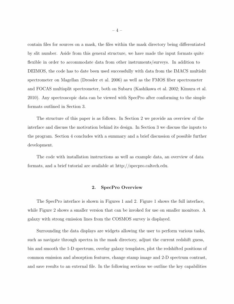
contain files for sources on a mask, the files within the mask directory being differentiated

by slit number. Aside from this general structure, we have made the input formats quite

flexible in order to accommodate data from other instruments/surveys. In addition to

DEIMOS, the code has to date been used successfully with data from the IMACS multislit

spectrometer on Magellan (Dressler et al. 2006) as well as the FMOS fiber spectrometer

and FOCAS multisplit spectrometer, both on Subaru (Kashikawa et al. 2002; Kimura et al.

2010). Any spectroscopic data can be viewed with SpecPro after conforming to the simple

formats outlined in Section 3.

The structure of this paper is as follows. In Section 2 we provide an overview of the

interface and discuss the motivation behind its design. In Section 3 we discuss the inputs to

the program. Section 4 concludes with a summary and a brief discussion of possible further

development.

The code with installation instructions as well as example data, an overview of data

formats, and a brief tutorial are available at http://specpro.caltech.edu.

2. SpecPro Overview

The SpecPro interface is shown in Figures 1 and 2. Figure 1 shows the full interface,

while Figure 2 shows a smaller version that can be invoked for use on smaller monitors. A

galaxy with strong emission lines from the COSMOS survey is displayed.

Surrounding the data displays are widgets allowing the user to perform various tasks,

such as navigate through spectra in the mask directory, adjust the current redshift guess,

bin and smooth the 1-D spectrum, overlay galaxy templates, plot the redshifted positions of

common emission and absorption features, change stamp image and 2-D spectrum contrast,

and save results to an external file. In the following sections we outline the key capabilities

– 5 –

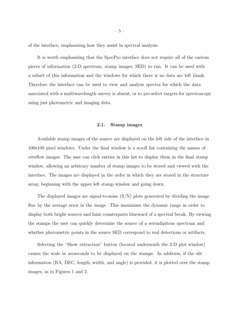
of the interface, emphasizing how they assist in spectral analysis.

It is worth emphasizing that the SpecPro interface does not require all of the various

pieces of information (2-D spectrum, stamp images, SED) to run. It can be used with

a subset of this information and the windows for which there is no data are left blank.

Therefore the interface can be used to view and analyze spectra for which the data

associated with a multiwavelength survey is absent, or to pre-select targets for spectroscopy

using just photometric and imaging data.

2.1. Stamp images

Available stamp images of the source are displayed on the left side of the interface in

100x100 pixel windows. Under the final window is a scroll list containing the names of

overflow images. The user can click entries in this list to display them in the final stamp

window, allowing an arbitrary number of stamp images to be stored and viewed with the

interface. The images are displayed in the order in which they are stored in the structure

array, beginning with the upper left stamp window and going down.

The displayed images are signal-to-noise (S/N) plots generated by dividing the image

flux by the average error in the image. This maximizes the dynamic range in order to

display both bright sources and faint counterparts blueward of a spectral break. By viewing

the stamps the user can quickly determine the source of a serendipitous spectrum and

whether photometric points in the source SED correspond to real detections or artifacts.

Selecting the “Show extraction” button (located underneath the 2-D plot window)

causes the scale in arcseconds to be displayed on the stamps. In addition, if the slit

information (RA, DEC, length, width, and angle) is provided, it is plotted over the stamp

images, as in Figures 1 and 2.

– 6 –

2.2. Spectrum Display

The one-dimensional spectrum is displayed in the upper right window of the display.

The spectrum is shown in white, with overlaid spectral templates shown in blue. Regions

of significant atmospheric absorption are indicated with horizontal blue lines. The residual

error, which can help determine whether a weak feature is real or an artifact due to sky

subtraction, can be overlaid on the plot by clicking the “Show sky” button on the second

row down from the 1-D display.

The 1-D spectrum can be binned and smoothed to bring out features in low S/N

spectra. Binning combines pixels, reducing the resolution of the spectrum to increase the

S/N, while smoothing performs an inverse variance weighted average in the vicinity of each

pixel to reduce the noise. In Figure 1 the spectrum has been binned and smoothed, clearly

revealing prominent emission features.

The 2-D spectrum is displayed beneath the 1-D spectrum, binned, if necessary, to

fit the display. The 2-D spectrum can be helpful to: (1) verify the fidelity of the 1-D

spectrum, (2) determine whether features observed in the 1-D spectrum are real or artifacts,

(3) identify serendipitous objects, and (4) examine the spatial morphology of emission

features. As described in Section 2.3, the user has the ability to reextract the 1-D spectrum

from the 2-D, which can be very useful in cases in which there was a problem with 1-D

extraction or the 1-D spectrum of a serendipitous source is desired.

The contrast of the 2-D spectrum can be adjusted with a slider widget. Next to the

contrast slider is a droplist widget labeled “Max sigma:”. This is set to 10 by default, which

indicates that contrast scaling has an upper limit of 10σ, so that pixels 10σ from the mean

are rescaled to the maximum pixel value of 255. Lowering this value can help in cases in

which the spectrum of interest is being drowned out by the light of bright serendipitous

sources.

– 7 –

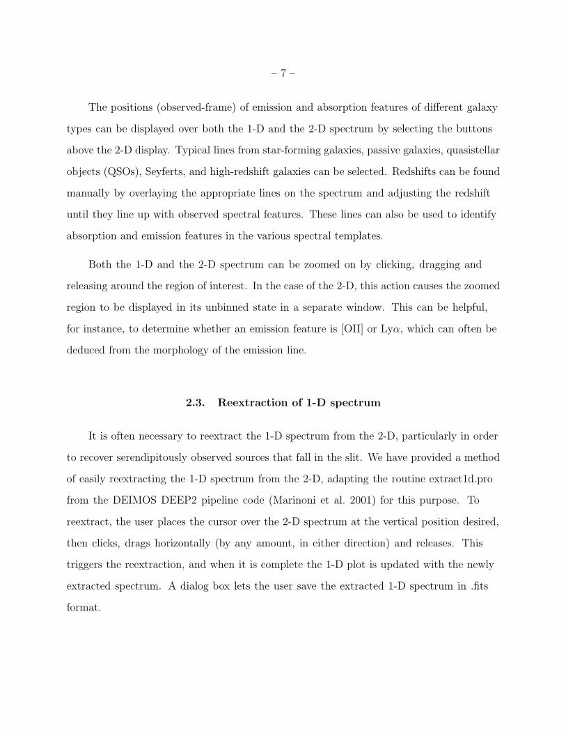
The positions (observed-frame) of emission and absorption features of different galaxy

types can be displayed over both the 1-D and the 2-D spectrum by selecting the buttons

above the 2-D display. Typical lines from star-forming galaxies, passive galaxies, quasistellar

objects (QSOs), Seyferts, and high-redshift galaxies can be selected. Redshifts can be found

manually by overlaying the appropriate lines on the spectrum and adjusting the redshift

until they line up with observed spectral features. These lines can also be used to identify

absorption and emission features in the various spectral templates.

Both the 1-D and the 2-D spectrum can be zoomed on by clicking, dragging and

releasing around the region of interest. In the case of the 2-D, this action causes the zoomed

region to be displayed in its unbinned state in a separate window. This can be helpful,

for instance, to determine whether an emission feature is [OII] or Lyα, which can often be

deduced from the morphology of the emission line.

2.3. Reextraction of 1-D spectrum

It is often necessary to reextract the 1-D spectrum from the 2-D, particularly in order

to recover serendipitously observed sources that fall in the slit. We have provided a method

of easily reextracting the 1-D spectrum from the 2-D, adapting the routine extract1d.pro

from the DEIMOS DEEP2 pipeline code (Marinoni et al. 2001) for this purpose. To

reextract, the user places the cursor over the 2-D spectrum at the vertical position desired,

then clicks, drags horizontally (by any amount, in either direction) and releases. This

triggers the reextraction, and when it is complete the 1-D plot is updated with the newly

extracted spectrum. A dialog box lets the user save the extracted 1-D spectrum in .fits

format.

– 8 –

2.4. SED

The source SED is displayed in the bottom right window of the interface. The

information for this plot comes from the photometry file, described in Section 3.5. The

plot extends from 0.1 to 10 µm and displays photometric AB magnitudes with errors. The

effective widths of the photometric bands are indicated with horizontal bars and errors

in the magnitude estimates are indicated with vertical bars. Observed-frame positions of

important SED features are indicated with vertical blue lines. These features include the

Lyman limit at 912 A, Lyα at 1216 A, the 4000 A break, and the typical SED peak of

evolved galaxies at 1.6 µm. The wavelength coverage of the spectrum is indicated with

vertical green lines.

2.5. Cross-Correlation

Automated redshift determination by convolution against spectral templates is a

powerful and time-saving capability. We have adapted cross-correlation routines originally

written for the SDSS spectral reduction package for use in SpecPro, with a library of

spectral templates available to correlate against (see Table 1). The templates span a

broad range of galaxy types. We have also included some stellar templates to help identify

high-redshift selected sources that are actually stars.

The user is expected to be able to choose an appropriate template based on the

spectrum and other information about the source. When one of the galaxy templates from

the template library is selected, the six best redshift matches are computed and the best

solution is displayed. The droplist “Auto-z solution:” under the 1-D spectrum contains all of

the solutions for examination. Clicking an alternate solution will switch to the new redshift

guess and move the template accordingly. Because the spectral template is overplotted on

– 9 –

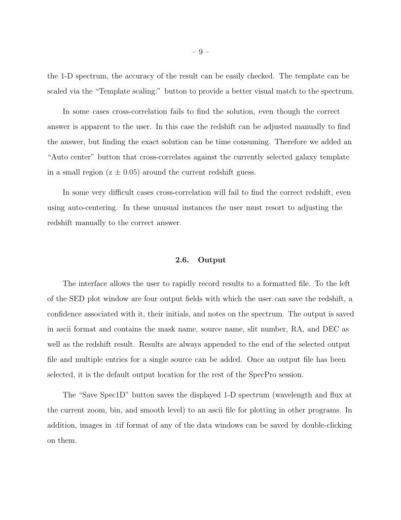
the 1-D spectrum, the accuracy of the result can be easily checked. The template can be

scaled via the “Template scaling:” button to provide a better visual match to the spectrum.

In some cases cross-correlation fails to find the solution, even though the correct

answer is apparent to the user. In this case the redshift can be adjusted manually to find

the answer, but finding the exact solution can be time consuming. Therefore we added an

“Auto center” button that cross-correlates against the currently selected galaxy template

in a small region (z ± 0.05) around the current redshift guess.

In some very difficult cases cross-correlation will fail to find the correct redshift, even

using auto-centering. In these unusual instances the user must resort to adjusting the

redshift manually to the correct answer.

2.6. Output

The interface allows the user to rapidly record results to a formatted file. To the left

of the SED plot window are four output fields with which the user can save the redshift, a

confidence associated with it, their initials, and notes on the spectrum. The output is saved

in ascii format and contains the mask name, source name, slit number, RA, and DEC as

well as the redshift result. Results are always appended to the end of the selected output

file and multiple entries for a single source can be added. Once an output file has been

selected, it is the default output location for the rest of the SpecPro session.

The “Save Spec1D” button saves the displayed 1-D spectrum (wavelength and flux at

the current zoom, bin, and smooth level) to an ascii file for plotting in other programs. In

addition, images in .tif format of any of the data windows can be saved by double-clicking

on them.

– 10 –

3. Data Formats

We have attempted to make the required formats simple and general so that data from

any instrument/survey can be easily adapted for use with SpecPro. While the files are

expected to be arranged by slit number, any sequential numbering scheme can be used to

differentiate sources. None of the inputs accepted by SpecPro are actually required for the

program to run; if one is missing, the corresponding field in the interface is left blank. The

program accepts the following five files:

• 1-D spectrum file (fits)

• 2-D spectrum file (fits)

• Stamp image file (fits)

• Photometry file (ascii)

• Information file (ascii)

These are briefly described in the rest of this section. More detailed descriptions are

given on the website, and example data is provided with the program download.

3.1. 1-D Spectrum

The 1-D spectrum is a stored as a structure with three fields: flux, ivar, and lambda.

Each field holds a one-dimensional double array. The flux field is the spectrum, the ivar

field is the inverse variance of the flux, and lambda is the wavelength at each pixel, in

angstroms. Note that the units of flux are arbitrary, but values proportional to Fν are

preferable because this matches the units of the spectral templates. The structure must be

saved in FITS format.

– 11 –

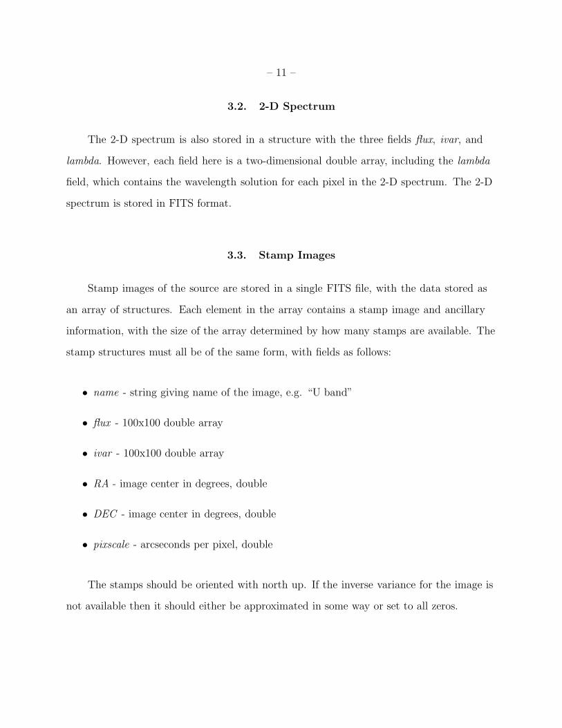
3.2. 2-D Spectrum

The 2-D spectrum is also stored in a structure with the three fields flux, ivar, and

lambda. However, each field here is a two-dimensional double array, including the lambda

field, which contains the wavelength solution for each pixel in the 2-D spectrum. The 2-D

spectrum is stored in FITS format.

3.3. Stamp Images

Stamp images of the source are stored in a single FITS file, with the data stored as

an array of structures. Each element in the array contains a stamp image and ancillary

information, with the size of the array determined by how many stamps are available. The

stamp structures must all be of the same form, with fields as follows:

• name - string giving name of the image, e.g. “U band”

• flux - 100x100 double array

• ivar - 100x100 double array

• RA - image center in degrees, double

• DEC - image center in degrees, double

• pixscale - arcseconds per pixel, double

The stamps should be oriented with north up. If the inverse variance for the image is

not available then it should either be approximated in some way or set to all zeros.

– 12 –

3.4. Information File

The information file contains ancillary information about a source displayed by the

interface and/or used in some of its functionality. This information includes source RA and

DEC, slit information, photometric redshift estimate, and other quantities (see the website

for a detailed description). If the user only has a subset of the information they can omit

the missing values, or set them to zero.

3.5. Photometry

The photometry file is a space delimited file with five columns: filter name, filter central

wavelength, effective filter bandwidth, AB magnitude, and AB magnitude error. Both the

filter central wavelength and effective filter bandwith should be expressed in angstroms.

Non-detections are indicated with an AB magnitude of -99, with the AB magnitude error

set to the lower bound on the AB magnitude established by the non-detection. Any

photometric point can be included, but the program’s SED plot extends from 0.1 to

10.0 µm.

4. Summary

SpecPro is an interactive IDL-based interface particularly suited to viewing astronomical

spectra in the context of multiwavelength surveys. In addition to 1-D and 2-D spectra,

the interface can display stamp images and the spectral energy distribution of the source.

Having all of this information in one display makes it much easier to identify the nature

and redshift of faint spectral targets.

We have made an effort to make the data formats required by the program both simple

– 13 –

and general. The program could potentially incorporate wrappers for various instrument’s

data or allow more flexible inputs; however, the effort required to achieve this flexibility is

probably too high considering the relative ease with which data can be made to conform

with the formats outlined in Section 3.

One possibility for future development is to incorporate tools for more detailed

spectroscopic analysis (line-fitting, determination of equivalent widths, etc.) from within

the interface. This was not the our intention when designing SpecPro, but the addition of

such functionality would make it a much more general tool for spectral analysis. Another

related possibility would be to allow the user to interactively fit the source SED from

within the interface, in order to determine galaxy stellar mass, age, and other parameters.

However, at present the interface is optimized for spectral classification and redshift

determination and we have no concrete plans for further development.

We have found the program valuable in our own analysis of DEIMOS spectra of targets

in the COSMOS survey field. In addition to making the identification of redshifts very

fast, it has also allowed us to efficiently characterize our sample and identify particularly

interesting galaxies for follow-up study. We feel that SpecPro will prove useful to others

working with spectroscopic samples as well.

The authors would like to thank Dr. Yuko Kakazu, Dr. Hai Fu, Dr. Lin Yan, and

Dr. Nick Scoville from the California Institute of Technology for their helpful comments

and suggestions during the development of the software. In addition, we would like to

acknowledge and thank Dr. Mara Salvato of the Max Planck Institute for Plasma Physics

and Dr. Francesca Civano of the Harvard-Smithsonian Center for Astronomy for providing

useful feedback on early versions of the code. We also thank Dr. Bahram Mobasher of the

University of California, Riverside for carefully reading a draft of this paper and making

suggestions that significantly improved its content.

– 14 –

SpecPro makes use of IDL code written and maintained by others. We thank Wayne

Landsman at NASA/GSFC for his work maintaining the IDL Astronomy User’s Library.

We also thank the authors of code we have used for our implementation of automated

cross-correlation, including David Schlegel, Doug Finkbeiner, Michael Cooper, and John

Johnson. We thank Craig Markwardt, whose MPFIT least-squares fitting package

(Markwardt 2009) is integral to the cross-correlatation functionality.

Finally, we thank an anonymous referee for carefully reading this manuscript and

providing very constructive feedback both in terms of content and with regard to the

distribution of the software on the web.

This work was supported in part by a visiting graduate student fellowship at the

Caltech Infrared Processing and Analysis Center (IPAC).

– 15 –

Fig. 1.— The SpecPro widget interface. The object shown is a star-forming galaxy at redshift

0.89. Stamp images of the source are displayed on the left side of the interface, and the 1-D

spectrum is displayed in the upper right window. On the 1-D plot, vertical lines mark the

positions of prominent emission features, and a spectral template is overlaid in blue. Under

the 1-D spectrum is the corresponding 2-D spectrum, binned to fit the display. The same

emission lines plotted over the 1-D spectrum are indicated in the 2-D spectrum, and the

atmospheric absorption regions are marked with horizontal red lines above and below the

spectrum. Emission lines ([OII], Hγ, Hβ, [OIII]) are easily visible in the binned 2-D image.

The window on the bottom right shows the SED of the source from the ultraviolet to the

mid-infrared. The AB magnitude (increasing downwards) is plotted against filter wavelength.

The SED data points indicate filter FWHM with horizontal bars and photometric errors with

vertical bars. The observed-frame positions of important photometric indicators, including

the Lyman limit at λ912 A, Lyα at λ1216 A, the 4000 A break, and 1.6 µm are indicated

with vertical dashed lines.

– 16 –

Fig. 2.— The SpecPro widget interface, small version. In this image, the “Show extraction”

button has been selected, causing the slit to be overlaid on the stamp images.

– 17 –

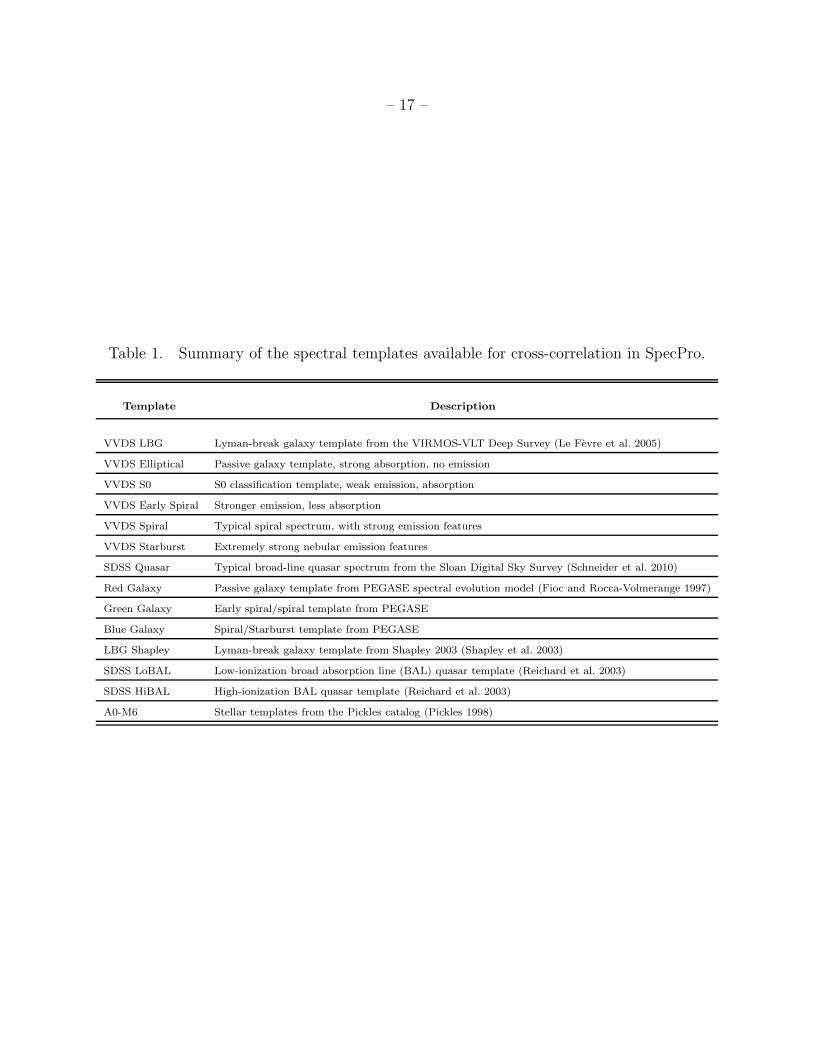
Table 1. Summary of the spectral templates available for cross-correlation in SpecPro.

Template Description

VVDS LBG Lyman-break galaxy template from the VIRMOS-VLT Deep Survey (Le Fevre et al. 2005)

VVDS Elliptical Passive galaxy template, strong absorption, no emission

VVDS S0 S0 classification template, weak emission, absorption

VVDS Early Spiral Stronger emission, less absorption

VVDS Spiral Typical spiral spectrum, with strong emission features

VVDS Starburst Extremely strong nebular emission features

SDSS Quasar Typical broad-line quasar spectrum from the Sloan Digital Sky Survey (Schneider et al. 2010)

Red Galaxy Passive galaxy template from PEGASE spectral evolution model (Fioc and Rocca-Volmerange 1997)

Green Galaxy Early spiral/spiral template from PEGASE

Blue Galaxy Spiral/Starburst template from PEGASE

LBG Shapley Lyman-break galaxy template from Shapley 2003 (Shapley et al. 2003)

SDSS LoBAL Low-ionization broad absorption line (BAL) quasar template (Reichard et al. 2003)

SDSS HiBAL High-ionization BAL quasar template (Reichard et al. 2003)

A0-M6 Stellar templates from the Pickles catalog (Pickles 1998)

– 18 –

REFERENCES

A. Dressler, T. Hare, B. C. Bigelow, and D. J. Osip. IMACS: the wide-field imaging spec-

trograph on Magellan-Baade. In Society of Photo-Optical Instrumentation Engineers

(SPIE) Conference Series, volume 6269 of Society of Photo-Optical Instrumentation

Engineers (SPIE) Conference Series, July 2006. doi: 10.1117/12.670573.

S. M. Faber, A. C. Phillips, R. I. Kibrick, B. Alcott, S. L. Allen, J. Burrous, T. Cantrall,

D. Clarke, A. L. Coil, D. J. Cowley, M. Davis, W. T. S. Deich, K. Dietsch, D. K.

Gilmore, C. A. Harper, D. F. Hilyard, J. P. Lewis, M. McVeigh, J. Newman,

J. Osborne, R. Schiavon, R. J. Stover, D. Tucker, V. Wallace, M. Wei, G. Wirth,

and C. A. Wright. The DEIMOS spectrograph for the Keck II Telescope: integration

and testing. In M. Iye & A. F. M. Moorwood, editor, Society of Photo-Optical

Instrumentation Engineers (SPIE) Conference Series, volume 4841 of Society

of Photo-Optical Instrumentation Engineers (SPIE) Conference Series, pages

1657–1669, March 2003. doi: 10.1117/12.460346.

M. Fioc and B. Rocca-Volmerange. PEGASE: a UV to NIR spectral evolution model of

galaxies. Application to the calibration of bright galaxy counts. A&A, 326:950–962,

October 1997.

M. Giavalisco, H. C. Ferguson, A. M. Koekemoer, M. Dickinson, D. M. Alexander,

F. E. Bauer, J. Bergeron, C. Biagetti, W. N. Brandt, S. Casertano, C. Cesarsky,

E. Chatzichristou, C. Conselice, S. Cristiani, L. Da Costa, T. Dahlen, D. de

Mello, P. Eisenhardt, T. Erben, S. M. Fall, C. Fassnacht, R. Fosbury, A. Fruchter,

J. P. Gardner, N. Grogin, R. N. Hook, A. E. Hornschemeier, R. Idzi, S. Jogee,

C. Kretchmer, V. Laidler, K. S. Lee, M. Livio, R. Lucas, P. Madau, B. Mobasher,

L. A. Moustakas, M. Nonino, P. Padovani, C. Papovich, Y. Park, S. Ravindranath,

A. Renzini, M. Richardson, A. Riess, P. Rosati, M. Schirmer, E. Schreier, R. S.

– 19 –

Somerville, H. Spinrad, D. Stern, M. Stiavelli, L. Strolger, C. M. Urry, B. Vandame,

R. Williams, and C. Wolf. The Great Observatories Origins Deep Survey: Initial

Results from Optical and Near-Infrared Imaging. ApJ, 600:L93–L98, January 2004.

doi: 10.1086/379232.

N. Kashikawa, K. Aoki, R. Asai, N. Ebizuka, M. Inata, M. Iye, K. S. Kawabata, G. Kosugi,

Y. Ohyama, K. Okita, T. Ozawa, Y. Saito, T. Sasaki, K. Sekiguchi, Y. Shimizu,

H. Taguchi, T. Takata, Y. Yadoumaru, and M. Yoshida. FOCAS: The Faint Object

Camera and Spectrograph for the Subaru Telescope. PASJ, 54:819–832, December

2002.

M. Kimura, T. Maihara, F. Iwamuro, M. Akiyama, N. Tamura, G. B. Dalton, N. Takato,

P. Tait, K. Ohta, S. Eto, D. Mochida, B. Elms, K. Kawate, T. Kurakami, Y. Moritani,

J. Noumaru, N. Ohshima, M. Sumiyoshi, K. Yabe, J. Brzeski, T. Farrell, G. Frost,

P. R. Gillingham, R. Haynes, A. M. Moore, R. Muller, S. Smedley, G. Smith,

D. G. Bonfield, C. B. Brooks, A. R. Holmes, E. Curtis Lake, H. Lee, I. J. Lewis,

T. R. Froud, I. A. Tosh, G. F. Woodhouse, C. Blackburn, R. Content, N. Dipper,

G. Murray, R. Sharples, and D. J. Robertson. Fibre Multi-Object Spectrograph

(FMOS) for the Subaru Telescope. PASJ, 62:1135–1147, October 2010.

O. Le Fevre, L. Guzzo, B. Meneux, A. Pollo, A. Cappi, S. Colombi, A. Iovino, C. Marinoni,

H. J. McCracken, R. Scaramella, D. Bottini, B. Garilli, V. Le Brun, D. Maccagni,

J. P. Picat, M. Scodeggio, L. Tresse, G. Vettolani, A. Zanichelli, C. Adami,

M. Arnaboldi, S. Arnouts, S. Bardelli, J. Blaizot, M. Bolzonella, S. Charlot,

P. Ciliegi, T. Contini, S. Foucaud, P. Franzetti, I. Gavignaud, O. Ilbert, B. Marano,

G. Mathez, A. Mazure, R. Merighi, S. Paltani, R. Pello, L. Pozzetti, M. Radovich,

G. Zamorani, E. Zucca, M. Bondi, A. Bongiorno, G. Busarello, F. Lamareille,

Y. Mellier, P. Merluzzi, V. Ripepi, and D. Rizzo. The VIMOS VLT deep survey.

– 20 –

The evolution of galaxy clustering to z ∼ 2 from first epoch observations. A&A, 439:

877–885, September 2005. doi: 10.1051/0004-6361:20041962.

C. Marinoni, M. Davis, A. L. Coil, and D. Finkbeiner. Spectral Reduction Software for the

DEEP2 Redshift Survey. ArXiv Astrophysics e-prints, September 2001.

C. B. Markwardt. Non-linear Least-squares Fitting in IDL with MPFIT. In D. A. Bohlender,

D. Durand, & P. Dowler, editor, Astronomical Society of the Pacific Conference

Series, volume 411 of Astronomical Society of the Pacific Conference Series, pages

251–+, September 2009.

A. J. Pickles. A Stellar Spectral Flux Library: 1150-25000 A. PASP, 110:863–878, July

1998. doi: 10.1086/316197.

T. A. Reichard, G. T. Richards, D. P. Schneider, P. B. Hall, A. Tolea, J. H. Krolik,

Z. Tsvetanov, D. E. Vanden Berk, D. G. York, G. R. Knapp, J. E. Gunn, and

J. Brinkmann. A Catalog of Broad Absorption Line Quasars from the Sloan Digital

Sky Survey Early Data Release. AJ, 125:1711–1728, April 2003. doi: 10.1086/368244.

D. P. Schneider, G. T. Richards, P. B. Hall, M. A. Strauss, S. F. Anderson, T. A. Boroson,

N. P. Ross, Y. Shen, W. N. Brandt, X. Fan, N. Inada, S. Jester, G. R. Knapp, C. M.

Krawczyk, A. R. Thakar, D. E. Vanden Berk, W. Voges, B. Yanny, D. G. York, N. A.

Bahcall, D. Bizyaev, M. R. Blanton, H. Brewington, J. Brinkmann, D. Eisenstein,

J. A. Frieman, M. Fukugita, J. Gray, J. E. Gunn, P. Hibon, Z. Ivezic, S. M.

Kent, R. G. Kron, M. G. Lee, R. H. Lupton, E. Malanushenko, V. Malanushenko,

D. Oravetz, K. Pan, J. R. Pier, T. N. Price, D. H. Saxe, D. J. Schlegel, A. Simmons,

S. A. Snedden, M. U. SubbaRao, A. S. Szalay, and D. H. Weinberg. The Sloan

Digital Sky Survey Quasar Catalog. V. Seventh Data Release. AJ, 139:2360–2373,

June 2010. doi: 10.1088/0004-6256/139/6/2360.

– 21 –

N. Scoville, H. Aussel, M. Brusa, P. Capak, C. M. Carollo, M. Elvis, M. Giavalisco,

L. Guzzo, G. Hasinger, C. Impey, J.-P. Kneib, O. LeFevre, S. J. Lilly, B. Mobasher,

A. Renzini, R. M. Rich, D. B. Sanders, E. Schinnerer, D. Schminovich, P. Shopbell,

Y. Taniguchi, and N. D. Tyson. The Cosmic Evolution Survey (COSMOS):

Overview. ApJS, 172:1–8, September 2007. doi: 10.1086/516585.

A. E. Shapley, C. C. Steidel, M. Pettini, and K. L. Adelberger. Rest-Frame Ultraviolet

Spectra of z˜3 Lyman Break Galaxies. ApJ, 588:65–89, May 2003. doi:

10.1086/373922.

This manuscript was prepared with the AAS LATEX macros v5.2.