A Likelihood Ratio Test of Independence of Componentsfor High-dimensional Normal Vectors

A PROJECT

SUBMITTED TO THE FACULTY OF THE GRADUATE SCHOOL

OF THE UNIVERSITY OF MINNESOTA

BY

Lin Zhang

IN PARTIAL FULFILLMENT OF THE REQUIREMENTS

FOR THE DEGREE OF

MASTER OF SCIENCE

Yongcheng Qi

May, 2013

c© Lin Zhang 2013

ALL RIGHTS RESERVED

Acknowledgements

I would like to thank my advisor, Yongcheng Qi for his support and guidance these

years. Thank Dr. Kang Ling James, she gave me cherished advise and encouragement

to my project and me. Thank Dr Barry James and Dr. Richard Green for serving

on my project committee, taking the time to read this paper, and hearing the defense.

Thank Xingguo Li, he helps me a lot on software use.

i

Dedication

To my dear mother.

ii

Abstract

Consider a p-variate normal population. We are interested in testing the indepen-

dence of its components based on a random sample of size n from this population. In

classic multivariate analysis, the dimension p is fixed or relatively small compared with

the sample size n, and the likelihood ratio test (LRT) is an effective way to test the

hypothesis of independence, and the limiting distribution of the LRT is a chi-squared

distribution. When p goes to infinity, the chi-square approximation of the LRT may

be invalid. In multivariate analysis, testing the independence of grouped components

is one topic of interest. When the grouping is well balanced and the number of groups

is fixed, the LRT, properly normalized, has a normal limit as proved in the literature.

In practice, grouping can be unbalanced, and the number of groups can be arbitrarily

large. In this project, we prove that the LRT statistic converges to a normal distribution

under quite general conditions. Simulation results including histograms and compar-

isons of sizes and powers of tests with those in the classical chi-square approximations

are presented as well.

Keywords: Likelihood ratio test, High-dimensional normal vector, Blocked Diagonal,

covariance matrix.

iii

Contents

Acknowledgements i

Dedication ii

Abstract iii

List of Tables vi

List of Figures vii

1 Introduction 1

1.1 Background . . . . . . . . . . . . . . . . . . . . . . . . . . . . . . . . . . 1

1.2 Discription of the Model . . . . . . . . . . . . . . . . . . . . . . . . . . . 2

2 Likelihood Ratio test 3

2.1 Likelihood Ratio Test . . . . . . . . . . . . . . . . . . . . . . . . . . . . 3

2.2 Wilks’ Statistic . . . . . . . . . . . . . . . . . . . . . . . . . . . . . . . . 5

3 Main Result 7

4 Some Lemmas 9

4.1 Multivariate Gamma Function and ξ(x) function . . . . . . . . . . . . . 9

4.2 Moment of Wilk’s Statistic . . . . . . . . . . . . . . . . . . . . . . . . . 11

4.3 Infinitesimal and estimates . . . . . . . . . . . . . . . . . . . . . . . . . 11

5 Proof of Theorem 17

iv

6 Simulation 21

References 23

v

List of Tables

6.1 Size and Power of LRT for Specified Normal Distribution . . . . . . . . 21

vi

List of Figures

6.1 Histograms of CLT and chi-square Approximation . . . . . . . . . . . . 22

vii

Chapter 1

Introduction

1.1 Background

In classic statistical inference, the likelihood ratio test (LRT) is one widely-used method

for hypothesis testing. An advantage of using the LRT is that one doesn’t have to esti-

mate the variance of the test statistics. It is well known that the asymptotic distribution

of the LRT is chi-square under certain regularity conditions when the dimension p is a

small constant or is negligible compared with the sample size n. However, the chi-square

approximation doesn’t fit the distribution of the LRT very well for the high-dimension

case, especially when p grows with the sample size n. For many modern datasets, their

dimensions can be proportionally large compared with the sample size. For example, fi-

nancial data, consumer data, modern manufacturing data and multimedia data all have

this feature. To deal with this feature, Schott(2001, 2005, 2007), Ledoit and Wolf(2002),

Bai et al.(2009), Chen et al(2010), Jiang et al (2012), and Jiang and Yang(2012) derived

different methods to study the classical likelihood ratio test when the dimension p is

large.

In this project, we are interested in testing the independence of grouped components

from a high dimensional normal vector. The same problem has been considered by Jiang

and Yang(2013), and Jiang and Qi (2013) when the number of the partition is fixed. The

aim of the project is to extend the test to an arbitrary partitions and allow the number

of the partition to change with the sample size n. The results are very applicable in

practice. For example, in the analysis of microarray data on genes, it is meaningful to

1

2

check whether there is correlation among pieces of genes.

1.2 Discription of the Model

This problem could be abstracted as the statistical model below. For a multivariate dis-

tribution Np(µ,Σ), we partition a set of p variates with a joint normal distribution into

k subsets and ask whether the k subsets are mutually independent, or equivalently, we

want to test whether variables among different subsets are dependent. More specifically,

let x1, x2, · · · , xn be i.i.d Rp-valued random vectors with normal distribution Np(µ,Σ).

We write the blocked diagonal covariance matrix Σ0 as

Σ0 =

Σ11 0 · · · 0

0 Σ22 · · · 0...

.... . .

...

0 0 · · · Σkk

.

Then we want to test the hypotheses

H0 : Σ = Σ0 vs Ha : Σ 6= Σ0. (1.1)

Let Wn be Wilks’ likelihood ratio test (LRT) statistic (to be given in (2.11)). The

traditional theory of multivariate analysis shows that −ρn logWn(Thereom 11.2.5 of

Muirhead(1982)) goes to a chi-square distribution when n tends to infinity and p is

fixed, where ρ is given in (2.12). Jiang and Yang(2013) showed that the chi-square

approximation is no longer true when p→∞. In fact, their results show that the central

limit theorem(CLT) holds, i.e. (logWn − µn)/σn actually converges to the standard

normal for a fixed number of partition k, where µn and σn can be expressed explicitly

as a function of sample size and partition.

In this project we will prove the CLT for the LRT, allowing that k changes with n

and the partition can be unbalanced in the sense that numbers of components within

subsets are not necessarily proportional.

The rest of the paper is organized as follows. In section 2, we introduce the LRT

and give a brief literature review. In section 3, we state our main result. In section 4,

we present a few lemmas, and in section 5, we provide the proof of the theorem given

in section 3.

Chapter 2

Likelihood Ratio test

2.1 Likelihood Ratio Test

Let the p-component vector x be distributed according to Np(µ,Σ). We partition x

into k subvectors.

x = (x(1), · · · ,x(k))′ (2.1)

where each x(i) has dimension qi respectively, with p =∑k

i=1 qi. The vector of means µ

and the covariance matrix Σ are partitioned similarly:

µ = (µ(1), · · · , µ(k))′ (2.2)

and

Σ =

Σ11 Σ12 · · · Σ1k

Σ21 Σ22 · · · Σ2k

· · · · · · · · · · · ·Σk1 Σk2 · · · Σkk

.

The null hypothesis is that the subvectors x(1), · · · ,x(k) are mutually independently

distributed, i.e, the density of x factors into the product of the density functions of

x(1), · · · ,x(k):

H0 : f(x|µ,Σ) =

k∏i=1

f(x(i)|µ(i),Σii). (2.3)

3

4

If x(1), · · ·x(k) are independent subvectors, then the covariance matrix is block diagonal

and denoted by Σ0:

Σ0 =

Σ11 0 · · · 0

0 Σ22 · · · 0

· · · · · · · · · · · ·0 0 · · · Σkk

with Σii unspecified for 1 ≤ i ≤ k. Given a sample of size n, x1, · · · ,xn are n observa-

tions on x, the likelihood ratio is

Λn =

maxµ,Σ0

L(µ,Σ0)

maxµ,Σ

L(µ,Σ), (2.4)

where

L(µ,Σ) =

n∏i=1

1

(2π)12p|Σ|

12

exp−1

2(xi − µ)′Σ−1(xi − µ). (2.5)

L(µ,Σ0) is L(µ,Σ) with Σij = 0, i 6= j, for all 0 ≤ i, j ≤ k; and the maximum is taken

with respect to all vectors µ and positive definite Σ and Σ0. According to Theorem

11.2.2 of Muirhead(1982), we have

maxµ,Σ

L(µ,Σ) =1

(2π)12pn|ΣΩ|

12n

exp−1

2pn, (2.6)

where

Σ =1

n− 1A =

1

n− 1

n∑i=1

(xi − x)′(xi − x). (2.7)

Under the null hypothesis,

maxµ,Σ0

L(µ,Σ0) =

k∏i=1

maxLi(µ(i),Σii)

=k∏i=1

1

(2π)12qin|Σii|

12n

exp−1

2qin

=1

(2π)12pn

k∏i=1

|Σii|12n

exp−1

2pn,

5

where

Σii =1

n− 1

n∑j=1

(x(i)j − x(i))(x

(i)j − x(i))′. (2.8)

If we partition A and Σ in the same way for Σ, we see that

Σii =1

n− 1Aii.

Then the likelihood ratio becomes

Λn =

maxµ,Σ0

L(µ,Σ0)

maxµ,Σ

L(µ,Σ)=

|ΣΩ|12n∏k

i=i |Σii|12n

=|A|

12n∏k

i=1 |Aii|12n. (2.9)

The critical region of the likelihood ratio test is

Λn ≤ Λn(α), (2.10)

where Λn(α) is a number such that the probability of (2.10) is α when∑

=∑

0.

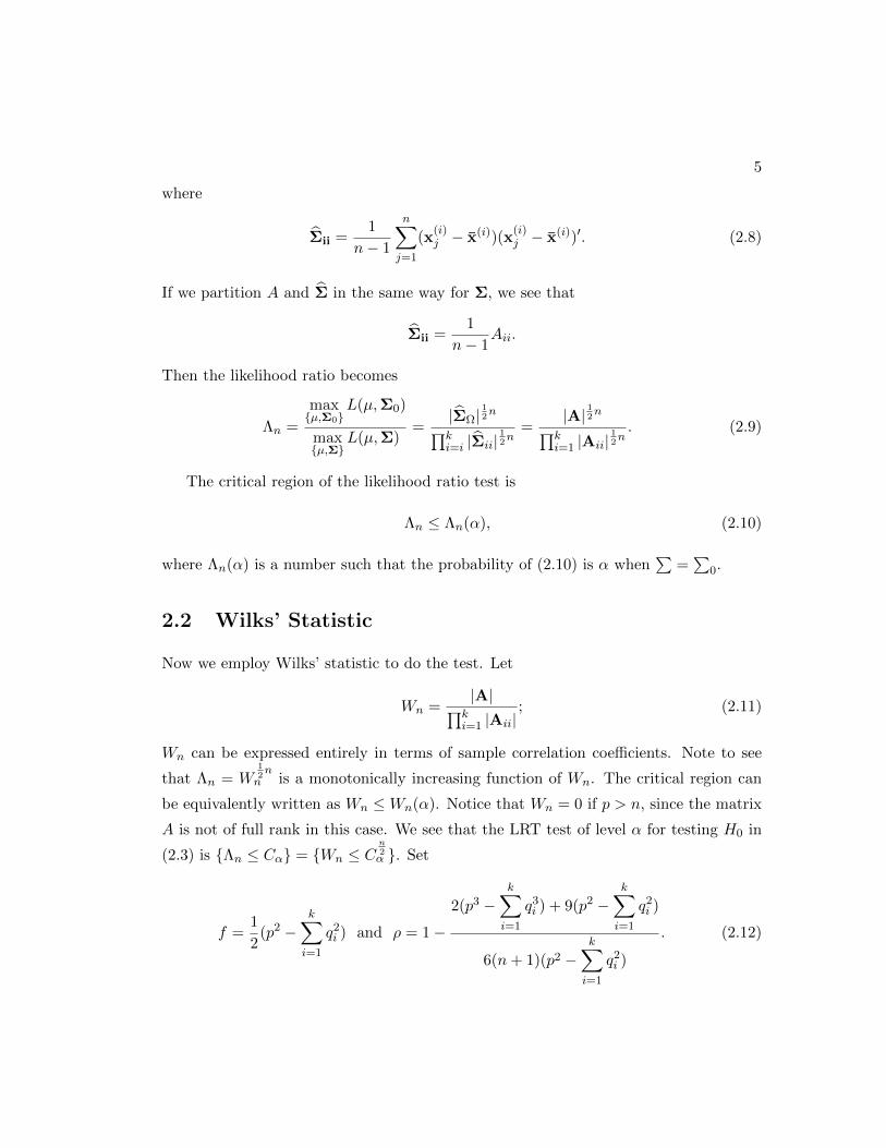
2.2 Wilks’ Statistic

Now we employ Wilks’ statistic to do the test. Let

Wn =|A|∏k

i=1 |Aii|; (2.11)

Wn can be expressed entirely in terms of sample correlation coefficients. Note to see

that Λn = W12n

n is a monotonically increasing function of Wn. The critical region can

be equivalently written as Wn ≤Wn(α). Notice that Wn = 0 if p > n, since the matrix

A is not of full rank in this case. We see that the LRT test of level α for testing H0 in

(2.3) is Λn ≤ Cα = Wn ≤ Cn2α . Set

f =1

2(p2 −

k∑i=1

q2i ) and ρ = 1−

2(p3 −k∑i=1

q3i ) + 9(p2 −

k∑i=1

q2i )

6(n+ 1)(p2 −k∑i=1

q2i )

. (2.12)

6

When n → ∞ while all qi’s remain fixed, the traditional χ2 approximation to the

distribution of Λn is found in Theorem 11.2.5 in Muirhead (1982):

−2ρ log(Λn)d−→ χ2

f .

When p is large enough or is proportional to n, this chi-square approximation may fail

(Jiang and Yang(2013)).

Considering the insufficiency of the LRT when p is large, Bai et al. (2009) introduced

a corrected likelihood ratio test for covariance matrices of Gaussian populations when

the dimension is large compared to the sample size. They also developed a LRT to fit

high-dimensional normal distribution Np(µ,Σ) with H0 : Σ = Ip. In their derivation,

the dimension p is no longer a fixed constant, but rather is a variable that goes to

infinity along with the sample size n, and the ratio between p = pn and converges to a

constant y, i.e.,

limn→∞

pnn

= y ∈ (0, 1)

Jiang and Yang (2013) further extended by Bai et al. (2009) to cover the case of y = 1,

and obtained the CLT of the LRT used for testing dependence of k groups of components

for high-dimensional datasets, where k is a fixed number.

Chapter 3

Main Result

In this chapter, we will give the main result of the project.

Let k ≥ 2, q1, · · · , qk be an arbitrary partition of dimension p. Denote p =∑k

i=1 qi,

and let

Σ = (Σij)p×p (3.1)

be the covariance matrix (positive definite), where Σij is a qi × qj sub-matrix for all

1 ≤ i, j ≤ k. Consider the following hypotheses,

H0 : Σ = Σ0 vs Ha : Σ 6= Σ0 (3.2)

which is equivalent to hypothesis (2.3). Let S be the sample covariance matrix. Then

partition A := (n− 1)S in the following way:A11 A12 · · · A1k

A21 A22 · · · A2k

......

. . ....

Ak1 Ak2 · · · Akk

where Aij is a qi × qj matrix. Wilks(1935) presented that the likelihood ratio statistic

for test (2.3)

Λn =|A|n/2∏k

i=1 |Aii|n/2= (Wn)n/2. (3.3)

When p > n+ 1, the matrix A is not full rank, therefore, Λn is degenerate.

We have the following theorem.

7

8

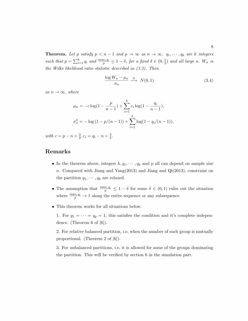
Theorem. Let p satisfy p < n − 1 and p → ∞ as n → ∞. q1, · · · , qk are k integers

such that p =∑k

i=1 qi and maxi qip ≤ 1 − δ, for a fixed δ ∈ (0, 1

2) and all large n. Wn is

the Wilks likelihood ratio statistic described as (3.3). Then

logWn − µnσn

d−→ N(0, 1) (3.4)

as n→∞, where

µn = −c log(1− p

n− 1) +

k∑i=1

ci log(1− qin− 1

),

σ2n = − log (1− p/(n− 1)) +

k∑i=1

log(1− qi/(n− 1)),

with c = p− n+ 32 , ci = qi − n+ 3

2 .

Remarks

• In the theorem above, integers k, q1, · · · , qk and p all can depend on sample size

n. Compared with Jiang and Yang(2013) and Jiang and Qi(2013), constraint on

the partition q1, · · · , qk are relaxed.

• The assumption that maxi qip ≤ 1 − δ for some δ ∈ (0, 1) rules out the situation

where maxi qip → 1 along the entire sequence or any subsequence.

• This theorem works for all situations below.

1. For q1 = · · · = qp = 1, this satisfies the condition and it’s complete indepen-

dence. (Theorem 6 of [6]).

2. For relative balanced partition, i.e, when the number of each group is mutually

proportional. (Theorem 2 of [6]).

3. For unbalanced partitions, i.e, it is allowed for some of the groups dominating

the partition. This will be verified by section 6 in the simulation part.

Chapter 4

Some Lemmas

4.1 Multivariate Gamma Function and ξ(x) function

For two sequences of numbers an and bn the notation an = O(bn) as n → ∞means lim sup(anbn ) < ∞. an = o(bn) as n → ∞ means lim an

bn= 0. an ∼ bn as n → ∞

stands for lim anbn

= 1.

Throughout the paper Γ(x) stands for the Gamma function defined on R, which

is defined via an improper integral that converges. Define the multivariate Gamma

function as:

Γp(x) := πp(p−1)/4p∏i=1

Γ(x− 1

2(i− 1)

)(4.1)

with x > (n− p)/2. See p. 62 in Muirhead (1982).

Define

ξ(x) = −2(log(1− x) + x), x ∈ [0, 1). (4.2)

ξ(x) is nonnegative in its domain. By the definition of ξ(x), ξ(0) = 0, and ξ′(x) = 2x1−x .

We have

ξ(x) = ξ(x)− ξ(0) =

∫ x

0ξ′(t)dt =

∫ x

0

2t

1− tdt

Substitute t = ux, then dt = xdu. Therefore

ξ(x) =

∫ 1

0

2ux2

1− uxdu = 2

∫ 1

0

ux2

1− uxdu. (4.3)

9

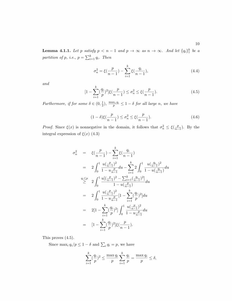
10

Lemma 4.1.1. Let p satisfy p < n − 1 and p → ∞ as n → ∞. And let qik1 be a

partition of p, i.e., p =∑k

i=1 qi. Then

σ2n = ξ(

p

n− 1)−

k∑i=1

ξ(qi

n− 1), (4.4)

and

[1−k∑i=1

(qip

)2]ξ(p

n− 1) ≤ σ2

n ≤ ξ(p

n− 1). (4.5)

Furthermore, if for some δ ∈ (0, 12), maxi qi

p ≤ 1− δ for all large n, we have

(1− δ)ξ( p

n− 1) ≤ σ2

n ≤ ξ(p

n− 1). (4.6)

Proof. Since ξ(x) is nonnegative in the domain, it follows that σ2n ≤ ξ( p

n−1). By the

integral expression of ξ(x) (4.3)

σ2n = ξ(

p

n− 1)−

k∑i=1

ξ(qi

n− 1)

= 2

∫ 1

0

u( pn−1)2

1− u pn−1

du−k∑i=1

2

∫ 1

0

u( qin−1)2

1− u( qin−1)

du

qi≤p≥ 2

∫ 1

0

u[( pn−1)2 −

∑ki=1( qi

n−1)2]

1− u( pn−1)

du

= 2

∫ 1

0

u( pn−1)2

1− u pn−1

[1−k∑i=1

(qip

)2]du

= 2[1−k∑i=1

(qip

)2]

∫ 1

0

u( pn−1)2

1− u pn−1

du

= [1−k∑i=1

(qip

)2]ξ(p

n− 1).

This proves (4.5).

Since maxi qi/p ≤ 1− δ and∑

i qi = p, we have

k∑i=1

(qip

)2 ≤ max qip

k∑i=1

qip

=max qip

≤ δ,

11

combined with (4.5), implying

σ2n ≥ (1− δ)ξ( p

n− 1).

This completes the proof of Lemma 4.1.1.

4.2 Moment of Wilk’s Statistic

Lemma 4.2.1. (Theorem 11.2.3 from Muirhead(1982)) Let p =∑k

i=1 qi and Wn be

Wilks’ likelihood ratio statistic defined as (3.3). Then

EW tn =

Γp(n−1

2 + t)

Γp(n−1

2 )

k∏i=1

Γqi(n−1

2 )

Γqi(n−1

2 + t)(4.7)

for any t > (p− n)/2, where Γp(x) is defined as (4.1).

4.3 Infinitesimal and estimates

Lemma 4.3.1. Let rn → ∞ and rn/n → 0 as n → ∞. Let q be a variable changing

according to n and rn ≤ q < n− 1.

limn→∞

suprn≤q<n−1

q(n−1)(n−1−q)

ξ( qn−1)

= 0. (4.8)

And furthermore,

limn→∞

suprn≤q<n−1

( q(n−1)(n−1−q))2

ξ( qn−1)

= 0. (4.9)

Proof. Set a = qn−1 , then it is needed to prove

suprn≤q<n−1

q(n−1)(n−1−q)

ξ( qn−1)

= suprn≤q<n−1

an−1−qξ(a)

→ 0.

Recall

ξ(x) = 2

∫ 1

0

ux2

1− uxdu = 2x2η(x),where η(x) =

∫ 1

0

u

1− uxdu.

η(x) is a monotonically increasing function and 12 ≤ η(x) ≤ ∞ for x ∈ [0, 1].

12

Let h be any positive constant in h ∈ (0, 12).

When rn ≤ q < h(n− 1), η(a) ≥ 12 and

suprn≤q<n−1

an−1−qξ(a)

≤ 2 suprn≤q<h(n−1)

1

n− 1− qn− 1

q

= 2 suprn≤q<h(n−1)

1

q(1− a)≤ 2

rn(1− h).

When h(n− 1) ≤ q ≤ (1− h)(n− 1), h ≤ a ≤ 1− h, we have

suph(n−1)≤q≤(1−h)(n−1)

an−1−qξ(a)

= suph(n−1)≤q≤(1−h)(n−1)

1

n− 1− q1

a

1∫ 10

u1−uadu

≤ suph(n−1)≤q≤(1−h)(n−1)

1

n− 1− q1

a

1∫ a0

11−tdt

= suph(n−1)≤q≤(1−h)(n−1)

1

n− 1− q1

alog(1− a)

= suph(n−1)≤q≤(1−h)(n−1)

1

n− 1

1

a

1

1− alog(1− a)

≤ 1

n− 1

1

h2log(1− h).

When (1− h)(n− 1) < q < n− 1,

sup(1−h)(n−1)<q<n−1

an−1−qξ(a)

≤ sup(1−h)(n−1)<q<n−1

1

1− h1

η(1− h).

Combining the 3 cases above and selecting hn = 1√n

, we get (4.7).

Sinceq

(n− 1)(n− q − 1)≤ 1 for rn ≤ q < n− 1

(4.8) follows from (4.7).

This completes the proof of Lemma 4.3.

Lemma 4.3.2. Let rn →∞ and rn/n→ 0 as n→∞. Then

q∑i=1

(1

n− i− 1

n− 1) = − log(1− q

n− 1)− q

n− 1+O(

q

(n− 1)(n− 1− q)) (4.10)

andq∑i=1

(log(n−1)−log(n−i) = (n−q− 1

2) log(1− q

n− 1)+q+O(

q

(n− 1)(n− q − 1)) (4.11)

uniformly on rn ≤ q < n− 1.

13

Proof. By the partial sum of harmonic series,

k∑i=1

1

i= log k + γ +

1

2k+ τ(k),

where γ is the Euler-Mascheroni constant and τ(k) = o( 1k2

) as k → ∞. See ”Sloane’s

A082912 : Sum of an terms of harmonic series is> 10n”, The On-Line Encyclopedia of

Integer Sequences. OEIS Foundation.

First, note that

q∑i=1

(1

n− i− 1

n− 1)

=n−1∑i=1

1

i−n−1−q∑i=1

1

i− q

n− 1

=− log(1− q

n− 1)− q

n− 1− q

2(n− 1)(n− 1− q)+ τ(n− 1− q).

To show (4.10), it suffices to show τ(n−1− q) = O( q(n−1)(n−1−q)). Note that τ(k) ≤ c

k2,

k ≥ 1 for some c > 0. We can also verify that

n− 1

q(n− 1− q)≤ 2.

As a result,

τ(n− 1− q) =n− 1

q(n− 1− q)q

(n− 1)(n− q − 1)≤ 2cq

(n− 1)(n− 1− q). (4.12)

This finishes the proof of (4.10).

To show (4.11), we apply the Stirling formula. Recall the Stirling formula from

Ahlfors(1979) is equivalent to

log Γ(x) = (x− 1

2) log(x)− x+

1

2log(2π) +

1

12x+O(

1

x2) (4.13)

as x→∞.

Take x = n− 1 and x = n− q− 1 respectively and take the difference, then we have

14

as n→∞,

log Γ(n− 1)− log Γ(n− q − 1)

=(n− 3

2) log(n− 1)− (n− q − 3

2) log(n− q − 1)− q

+1

12(

1

n− 1− 1

n− q − 1) +O(

1

(n− 1)2) +O(

1

(n− q − 1)2)

=(n− 3

2) log(n− 1)− (n− q − 3

2) log(n− q − 1)− q

− q

12(n− 1)(n− q − 1)+O(

1

(n− 1)2) +O(

1

(n− q − 1)2)

=(n− 3

2) log(n− 1)− (n− q − 3

2) log(n− q − 1)− q

+O(q

(n− 1)(n− q − 1)).

In the last step, we have used the following estimate

1

(n− 1)2+

1

(n− q − 1)2= O(

q

(n− 1)(n− q − 1)). (4.14)

For any rn ≤ q < n− 1, uniformly,

1

(n− 1)2≤ q

(n− 1)(n− q − 1)

which, combined with (4.11), gives (4.13).

Note that for any integer m ≥ 1, Γ(m) = (m− 1)!. Then we have

q∑i=1

(log(n− 1)− log(n− i))

=q log(n− 1)− (log Γ(n− 1)− log Γ(n− q − 1)) + log(1− q

n− 1)

=q log(n− 1)− (n− 3

2) log(n− 1) + (n− q − 3

2) log(n− q − 1) + q

+O(q

(n− 1)(n− q − 1)) + log(1− q

n− 1)

=(n− q − 1

2) log(1− q

n− 1) + q +O(

q

(n− 1)(n− q − 1)).

This finishes the proof of (4.11).

15

Lemma 4.3.3. (Lemma 2.1 from Jiang and Qi(2013)) Let b := b(x) be a real-valued

function defined on (0,∞).

logΓ(x+ b)

Γ(x)= (x+ b) log(x+ b)− x log x− b− b

2x+O(

b2 + |b|+ 1

x2) (4.15)

holds uniformly on b ∈ [−lx, lx] for any given constant l ∈ (0, 1). Furthermore, as

x→∞,

log[Γ(x+ b)

Γ(x)· Γ(z)

Γ(z + b)] = b(log x−log z)+

b2 − b2

(1

x−1

z)+O(

|b|3(x− z)x3

)+O(b2 + |b|+ 1

x2)

(4.16)

uniformly over b ∈ [−lx/2, lx/2] and z ∈ [x/2, x] for any l ∈ (0, 1).

Lemma 4.3.4. Let t = tn be a bounded variable with respect to n. Let rn → ∞ and

rn/n→ 0 as n→∞. Then

log [Γ(n−1

2 )

Γ(n−12 + t)

]qΓq(

n−12 + t)

Γq(n−1

2 )

=t[(q − n+3

2) log(1− q

n− 1)− n− 2

n− 1q] + t2

ξ( qn−1)

2

+O(q

(n− 1)(n− q − 1))(t+ t2) +O(

|t|3q2

n3) +O(

q(|t|2 + |t|+ 1)

n2).

holds uniformly for rn ≤ q < n− 1.

Proof. From the definition of Γp(x) in (4.1) we have

log [Γ(n−1

2 )

Γ(n−12 + t)

]qΓq(

n−12 + t)

Γq(n−1

2 )= −

q∑i=1

log [Γ(n−1

2 + t)

Γ(n−12 )

Γ(n−i2 )

Γ(n−i2 + t)]. (4.17)

By applying Lemma 4.3.3 to the summands, we have

log[Γ(n−1

2 + t)

Γ(n−1

2

) ·Γ(n−i

2

)Γ(n−i

2 + t) ]

= t(logn− 1

2− log

n− i2

) + (t2 − t)( 1

n− 1− 1

n− i)

+O(|t|3(i− 1)

n3) +O(

|t|2 + |t|+ 1

n2)

= t(log(n− 1)− log(n− i)− (1

n− 1− 1

n− i))

+ t2(1

n− 1− 1

n− i) +O(

|t|3(i− 1)

n3) +O(

|t|2 + |t|+ 1

n2)

16

uniformly for 1 ≤ i ≤ q. Then by Lemma 4.3.2,

q∑i=1

log [Γ(n−1

2 + t)

Γ(n−12 )

Γ(n−i2 )

Γ(n−i2 + t)]

=t(

q∑i=1

[log(n− 1)− log(n− i)] +

q∑i=1

(1

n− i− 1

n− 1))

− t2q∑i=1

(1

n− i− 1

n− 1) +O(

q∑i=1

(|t|3(i− 1)

n3)) +O(

q(|t|2 + |t|+ 1)

n2)

=t[(n− q − 1

2) log(1− q

n− 1) + q +O(

q

(n− 1)(n− q − 1))− log(1− q

n− 1)

− q

n− 1]− t2[

1

2ξ(

q

n− 1)−O(

q

(n− 1)(n− 1− q))] +O(

|t|3q(q − 1)/2

n3)

+O(q(|t|2 + |t|+ 1)

n2)

=− t[(q − n+3

2) log(1− q

n− 1)− n− 2

n− 1q]− t[O(

q

(n− 1)(n− q − 1))]

−t2[1

2ξ(

q

n− 1)]− t2[O(

q

(n− 1)(n− 1− q))]

+[O(|t|3q2

n3) +O(

q(|t|2 + |t|+ 1)

n2)],

which together with (4.17) completes the proof of the lemma.

Chapter 5

Proof of Theorem

To prove (3.4), it suffices to show that

E exp[( logWn − µn

σn

)s] = exp (−µns

σn)E[W

sσnn ] −→ es

2/2

as n→∞ for all s such that |s| ≤ 1 and for corresponding µn and σn, or equivalently

logEW tn = µnt+

σ2nt

2

2+ o(1) (5.1)

as n→∞ with |σnt| ≤ 1. By Lemma 4.2.1,

EW tn =

Γp(n−1

2 + t)

Γp(n−1

2 )

k∏i=1

Γqi(n−1

2 )

Γqi(n−1

2 + t)

= [Γ(n−1

2 )

Γ(n−12 + t)

]pΓp(

n−12 + t)

Γp(n−1

2 )/

k∏i=1

[Γ(n−1

2 )

Γ(n−12 + t)

]qiΓqi(

n−12 + t)

Γqi(n−1

2 ).

By taking logarithms on both sides, we have

logEW tn = −

p∑i=1

log[Γ(n−1

2 + t)

Γ(n−1

2

) Γ(n−i

2

)Γ(n−i

2 + t) ] +

k∑i=1

qi∑j=1

log[Γ(n−1

2 + t)

Γ(n−1

2

) Γ(n−j

2

)Γ(n−j

2 + t) ].

(5.2)

17

18

For the first sum of the right hand side, set c = p − n + 32 and g(t) = t2 + |t| + 1. By

Lemma 4.3.4 with q = p, we have

−p∑i=1

log[Γ(n−1

2 + t)

Γ(n−1

2

) Γ(n−i

2

)Γ(n−i

2 + t) ]

=t[c log(1− p

n− 1)− n− 2

n− 1p] +

t2

2ξ(

p

n− 1)

+(t+ t2)O(p

(n− 1)(n− p− 1)) +O(

|t|3p2

n3) +O(

pg(t)

n2)

=t[c log(1− p

n− 1)]− tn− 2

n− 1p+

t2

2ξ(

p

n− 1)

+(t+ t2)O(p

(n− 1)(n− p− 1)) +O(

pg(t)

n2).

For the second sum on the right hand side of (5.2), we set ci = qi − n+ 32 and note

that p =∑

i qi and maxi qip ≤ 1 − δ for some δ ∈ (0, 1

2). Again using Lemma 4.3.4 with

q = qi, we have

k∑i=1

qi∑j=1

log[Γ(n−1

2 + t)

Γ(n−1

2

) Γ(n−j

2

)Γ(n−j

2 + t) ]

=−k∑i=1

t[ci log(1− qin− 1

)− n− 2

n− 1qi] +

t2

2ξ(

qin− 1

)

−(t+ t2)k∑i=1

O(qi

(n− 1)(n− 1− qi)) +O(

|t|3∑

i q2i

n3) +O(

pg(t)

n2)

=t[−k∑i=1

ci log(1− qin− 1

)] + tn− 2

n− 1p− t2

2

k∑i=1

ξ(qi

n− 1)

−(t+ t2)k∑i=1

O(qi

(n− 1)(n− 1− qi)) +O(

pg(t)

n2).

19

Therefore,

logEW tn = t[c log(1− p

n− 1)−

k∑i=1

ci log(1− qin− 1

)] +t2

2[ξ(

p

n− 1)−

k∑i=1

ξ(qi

n− 1)]

+ (t+ t2)[O(p

(n− 1)(n− p− 1)) +

k∑i=1

O(qi

(n− 1)(n− 1− qi))] +O(

pg(t)

n2)

= tµn +t2

2σ2n

+ (t+ t2)[O(p

(n− 1)(n− p− 1)) +

k∑i=1

O(qi

(n− 1)(n− 1− qi))] +O(

pg(t)

n2),

where

µn = −c log(1− p

n− 1) + ci

k∑i=1

log(1− qin− 1

),

σ2n = ξ(

p

n− 1)−

k∑i=1

ξ(qi

n− 1).

Now it is sufficient to prove as n→∞,

(t+ t2)[O(p

(n− 1)(n− p− 1)) +

k∑i=1

O(qi

(n− 1)(n− 1− qi))] +O(

pg(t)

n2) = o(1) (5.3)

for all |σnt| ≤ 1. Recall the constraint that p ≤ n − 2, p → ∞ and maxi qip ≤ 1 − δ for

some δ ∈ (0, 12).

We can verify that

k∑i=1

O(qi

(n− 1)(n− 1− qi)) ≤

k∑i=1

O(qi

(n− 1)(n− 1− p))

≤ O(

∑qi

(n− 1)(n− 1− p)) = O(

p

(n− 1)(n− 1− p)).

Equation (5.3) becomes

(t+ t2)O(p

(n− 1)(n− p− 1)) +O(

pg(t)

n2) = o(1). (5.4)

From (4.5), we have

|t| ≤ | 1

σn| = O(

1√ξ( pn−1)

).

20

By (4.8) and (4.9) of Lemma 4.3.1 with q = p,

t[O(p

(n− 1)(n− 1− p))] = O(

p(n−1)(n−1−p)√

ξ( pn−1)

) = o(1), (5.5)

t2[O(p

(n− 1)(n− 1− p))] = O(

p(n−1)(n−1−p)

ξ( pn−1)

) = o(1). (5.6)

Recall g(t) = t2 + |t| + 1 and for any p → ∞ and p < n − 1, ξ( pn−1) = O(( p

n−1)2),

with pn−1 ≤ θ, when θ is small in θ ∈ (0, 1). Then

O(pg(t)

n2) = O(

pt2

n2) +O(

p|t|n2

) +O(p

n2)

= O(p

n2

(n− 1)2

p2) +O(

p

n2

n− 1

p) + o(1)

= O(1

p) +O(

1

n) + o(1) = o(1).

Also when θ ≤ pn−1 ≤ 1, by the increasing property of ξ(x) in (4.2),

pt2

n2≤ p

n2/ξ(

p

n− 1) ≤ p

n2/ξ(θ)→ 0.

Similarlypt

n2≤ p

n2/

√ξ(

p

n− 1) ≤ p

n2/√ξ(θ)→ 0,

and

O(pg(t)

n2) = O(

pt2

n2) +O(

p|t|n2

) +O(p

n2) = o(1).

This completes the proof of (3.4).

Chapter 6

Simulation

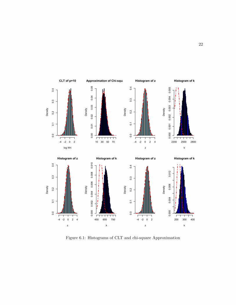
In this section, we compare the performance of the chi-square approximation and the

normal approximation through a finite sample simulation study. We plot the histograms

for the chi-square statistics which are used for the chi-square approximation and compare

with their corresponding limiting chi-square curves. Similarly, we plot the histograms of

the statistic which is used for the normal approximation and compare with the standard

normal curve.

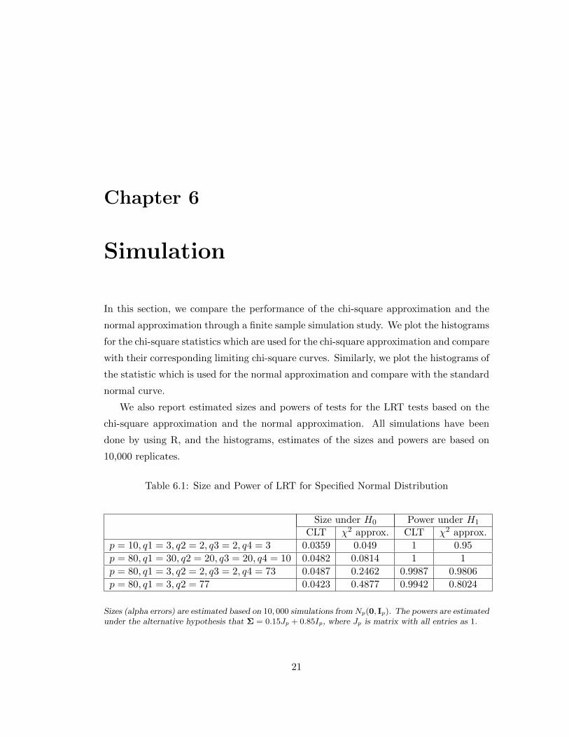
We also report estimated sizes and powers of tests for the LRT tests based on the

chi-square approximation and the normal approximation. All simulations have been

done by using R, and the histograms, estimates of the sizes and powers are based on

10,000 replicates.

Table 6.1: Size and Power of LRT for Specified Normal Distribution

Size under H0 Power under H1

CLT χ2 approx. CLT χ2 approx.

p = 10, q1 = 3, q2 = 2, q3 = 2, q4 = 3 0.0359 0.049 1 0.95

p = 80, q1 = 30, q2 = 20, q3 = 20, q4 = 10 0.0482 0.0814 1 1

p = 80, q1 = 3, q2 = 2, q3 = 2, q4 = 73 0.0487 0.2462 0.9987 0.9806

p = 80, q1 = 3, q2 = 77 0.0423 0.4877 0.9942 0.8024

Sizes (alpha errors) are estimated based on 10, 000 simulations from Np(0, Ip). The powers are estimatedunder the alternative hypothesis that Σ = 0.15Jp + 0.85Ip, where Jp is matrix with all entries as 1.

21

22

CLT of p=10

log Wn

Density

-4 -2 0 2

0.0

0.1

0.2

0.3

0.4

Approximation of Chi-squareDensity

10 30 50 70

0.00

0.01

0.02

0.03

0.04

0.05

Histogram of z

z

Density

-4 -2 0 2 4

0.0

0.1

0.2

0.3

0.4

Histogram of k

k

Density

2200 2500 2800

0.000

0.001

0.002

0.003

0.004

0.005

Histogram of z

z

Density

-4 -2 0 2 4

0.0

0.1

0.2

0.3

0.4

Histogram of k

k

Density

450 600 750

0.000

0.002

0.004

0.006

0.008

0.010

Histogram of z

z

Density

-4 -2 0 2

0.0

0.1

0.2

0.3

0.4

Histogram of k

k

Density

200 300 400

0.000

0.004

0.008

0.012

Figure 6.1: Histograms of CLT and chi-square Approximation

References

[1] Ahlfors, L.V(1979), Complex Analysis McGraw-Hill, Inc., 3rd Ed.

[2] Anderson, T. W.(1984) An Introduction to Multivariate Statistical Analysis. 2nd

Ed John Wiley & Sons..

[3] Bai, Z., Jiang, D., Yao, J. and Zheng, S. (2009). Corrections to LRT on large

dimensional covariance matrix by RMT. J. Royal Stat. Soc., Ser. B16, 296-298.

[4] Chen, S., Zhang, L., and Zhong, P. (2010). Tests for highdimensional covariance

matrices. J. Amer. Stat. Assoc. 105, 810-819.

[5] Ledoit, O. and Wolf, M. (2002) Some hypothesis test for the covariance matrix when

the dimension is large compared to the sample size. Ann. Statist. 30,1081-1102.

[6] Jiang, D., Jiang, T. and Yang, F.(2012) Likelihood ratio tests for covariance matri-

ces of high-dimensional normal distributions. J. Stat. Plann. Inference 142, 2241-

2256.

[7] Jiang, T. and Yang, F.(2013) Central limit theorems for classical likelihood ratio

tests for high-dimensional normal distributions. Ann of Statistics.

[8] Jiang, T. and Qi, Yongcheng.(2013) Central limit theorems for classical likelihood

ratio tests for high-dimensional normal distributions II. Preprint.

[9] Morrison, D. F. (2004). Multivariate Statistical Methods. Duxbury Press, 4th Ed.

[10] Muirhead, R. J. (1982). Aspects of Multivariate Statistical Theory. Wiley, New

York.

23

24

[11] Schott, J.R.(2007). A test for the equality of covariance matrices when the dimen-

sion is large relative to the sample sizes. Comput. Statist. Data Anal. 51, 6535-6542.

[12] Schott, J. R. (2005). Testing for complete independence in high dimensions.

Biometrika 92, 951-956.

[13] Schott, J. R. (2001). Some tests for the equality of covariance matrices. J. Stat.

Plann. Inference 94, 25-36.

[14] Wilks, S. S. (1935). On the independence of k sets of normally distributed statistical

variables.Econometrica 3, 309-326.