solving variational inequalities with stochastic mirror-prox algorithm

SOLVING VARIATIONAL INEQUALITIES WITH STOCHASTICMIRROR-PROX ALGORITHM

ANATOLI JUDITSKY∗, ARKADI NEMIROVSKI† , AND CLAIRE TAUVEL‡

June 2, 2008Abstract. In this paper we consider iterative methods for stochastic variational inequalities

(s.v.i.) with monotone operators. Our basic assumption is that the operator possesses both smoothand nonsmooth components. Further, only noisy observations of the problem data are available. Wedevelop a novel Stochastic Mirror-Prox (SMP) algorithm for solving s.v.i. and show that with theconvenient stepsize strategy it attains the optimal rates of convergence with respect to the prob-lem parameters. We apply the SMP algorithm to Stochastic composite minimization and describeparticular applications to Stochastic Semidefinite Feasability problem and Eigenvalue minimization.

Key words. Nash variational inequalities, stochastic convex-concave saddle-point problem,large scale stochastic approximation, reduced complexity algorithms for convex optimization

AMS subject classifications. 90C15, 65K10, 90C47

1. Introduction. Let Z be a convex compact set in Euclidean space E withinner product 〈·, ·〉, ‖ · ‖ be a norm on E (not necessarily the one associated with theinner product), and F : Z → E be a monotone mapping:

∀(z, z′ ∈ Z) : 〈F (z)− F (z′), z − z′〉 > 0)(1.1)

We are interested to approximate a solution to the variational inequality (v.i.)

find z∗ ∈ Z : 〈F (z), z∗ − z〉 6 0 ∀z ∈ Z(1.2)

associated with Z, F . Note that since F is monotone on Z, the condition in (1.2) isimplied by 〈F (z∗), z − z∗〉 > 0 for all z ∈ Z, which is the standard definition of a(strong) solution to the v.i. associated with Z, F . The inverse – a solution to v.i. asdefined by (1.2) (a “weak” solution) is a strong solution as well – also is true, provided,e.g., that F is continuous. An advantage of the concept of weak solution is that sucha solution always exists under our assumptions (F is well defined and monotone on aconvex compact set Z).

We quantify the inaccuracy of a candidate solution z ∈ Z by the error

Errvi(z) := maxu∈Z

〈F (u), z − u〉;(1.3)

note that this error is always > 0 and equals zero iff z is a solution to (1.2).In what follows we impose on F , aside of the monotonicity, the requirement

∀(z, z′ ∈ Z) : ‖F (z)− F (z′)‖∗ 6 L‖z − z′‖+ M(1.4)

with some known constants L > 0,M > 0. From now on,

‖ξ‖∗ = maxz:‖z‖61

〈ξ, z〉(1.5)

∗LJK, Universite J. Fourier, B.P. 53, 38041 Grenoble Cedex 9, France, [email protected]†Georgia Institute of Technology, Atlanta, Georgia 30332, USA, [email protected],

research of this author was partly supported by the NSF award DMI-0619977.‡LJK, Universite J. Fourier, B.P. 53, 38041 Grenoble Cedex 9, France, [email protected]

1

2 A. JUDITSKY, A. NEMIROVSKI AND C. TAUVEL

is the norm conjugate to ‖ · ‖.We are interested in the case where (1.2) is solved by an iterative algorithm based

on a stochastic oracle representation of the operator F (·). Specifically, when solvingthe problem, the algorithm acquires information on F via subsequent calls to a blackbox (“stochastic oracle”, SO). At i-th call, i = 0, 1, ..., the oracle gets as input asearch point zi ∈ Z (this point is generated by the algorithm on the basis of theinformation accumulated so far) and returns the vector Ξ(zi, ζi), where ζi ∈ RN∞i=1

is a sequence of i.i.d. (and independent of the queries of the algorithm) randomvariables. We suppose that the Borel function Ξ(z, ζ) is such that

∀z ∈ Z : E Ξ(z, ζ1) = F (z), E‖Ξ(z, ζi)− F (z)‖2∗

6 σ2.(1.6)

We call a monotone v.i. (1.1), augmented by a stochastic oracle (SO), a stochasticmonotone v.i. (s.v.i.).

To motivate our goal, let us start with known results [6] on the limits of perfor-mance of iterative algorithms for solving large-scale stochastic v.i.’s. To “normalize”the situation, assume that Z is the unit Euclidean ball in E = Rn and that n islarge. In this case, the rate of convergence of a whatever algorithm for solving v.i.’scannot be better than O(1)

[Lt + M+σ√

t

]. In other words, for a properly chosen pos-

itive absolute constant C, for every number of steps t, all large enough values of nand any algorithm B for solving s.v.i.’s on the unit ball of Rn, one can point outa monotone s.v.i. satisfying (1.4), (1.6) and such that the expected error of theapproximate solution zt generated by B after t steps , applied to such s.v.i., is at leastc[

Lt + M+σ√

t

]for some c > 0. To the best of our knowledge, no one of existing algo-

rithms allows to achieve, uniformly in the dimension, this convergence rate. In fact,the “best approximations” available are given by Robust Stochastic Approximation(see [3] and references therein) with the guaranteed rate of convergence O(1)L+M+σ√

t

and extra-gradient-type algorithms for solving deterministic monotone v.i.’s with Lip-schitz continuous operators (see [7, 10, 11, 12]), which attains the accuracy O(1)L

t inthe case of M = σ = 0 or O(1) M√

twhen L = σ = 0.

The goal of this paper is to demonstrate that a specific Mirror-Prox algorithm [7]for solving monotone v.i.’s with Lipschitz continuous operators can be extended ontomonotone s.v.i.’s to yield, uniformly in the dimension, the optimal rate of convergenceO(1)

[Lt + M+σ√

t

]. We present the corresponding extension and investigate it in details:

we show how the algorithm can be “tuned” to the geometry of the s.v.i. in question,derive bounds for the probability of large deviations of the resulting error, etc. We alsopresent a number of applications where the specific structure of the rate of convergenceindeed “makes a difference”.

The main body of the paper is organized as follows: in Section 2, we describeseveral special cases of monotone v.i.’s we are especially interested in (convex Nashequilibria, convex-concave saddle point problems, convex minimization). We singleout these special cases since here one can define a useful “functional” counterpartErrN(·) of the just defined error Errvi(·); both ErrN and Errvi will participate inour subsequent efficiency estimates. Our main development – the Stochastic MirrorProx (SMP) algorithm – is presented in Section 3. Some general results obout theperformance of the SMP are presented in Section 3.2. Then in Section 4 we presentSMP for Stochastic composite minimization and discuss its applications to StochasticSemidefinite Feasability problem and Eigenvalue minimization. All technical proofsare collected in the appendix.

STOCHASTIC MIRROR-PROX ALGORITHM 3

Notations. In the sequel, lowercase Latin letters denote vectors (and sometimesmatrices). Script capital letters, like E , Y, denote Euclidean spaces; the inner productin such a space, say, E , is denoted by 〈·, ·〉E (or merely 〈·, ·〉, when the correspondingspace is clear from the context). Linear mappings from one Euclidean space to an-other, say, from E to F , are denoted by boldface capitals like A (there are also somereserved boldface capitals, like E for expectation, Rk for the k-dimensional coordi-nate space, and Sk for the space of k × k symmetric matrices). A∗ stands for theconjugate to mapping A: if A : E → F , then A∗ : F → E is given by the identity〈f,Ae〉F = 〈A∗f, e〉E for f ∈ F , e ∈ E . When both the origin and the destinationspace of a linear map, like A, are the standard coordinate spaces, the map is identifiedwith its matrix A, and A∗ is identified with AT . For a norm ‖ · ‖ on E , ‖ · ‖∗ standsfor the conjugate norm, see (1.5).

For Euclidean spaces E1, ..., Em, E = E1 × ...× Em denotes their Euclidean directproduct, so that a vector from E is a collection u = [u1; ...;um] (“MATLAB notation”)of vectors u` ∈ E`, and 〈u, v〉E =

∑`〈u`, v`〉E`

. Sometimes we allow ourselves to write(u1, ..., um) instead of [u1; ...; um].

2. Preliminaries.

2.1. Nash v.i.’s and functional error. In the sequel, we shall be especiallyinterested in a special case of v.i. (1.2) – in a Nash v.i. coming from a convexNash Equilibrium problem, and in the associated functional error measure. The NashEquilibrium problem can be described as follows: there are m players, i-th of themchoosing a point zi from a given set Zi. The loss of i-th player is a given functionφi(z) of the collection z = (z1, ..., zm) ∈ Z = Z1 × ... × Zm of player’s choices. Withslight abuse of notation, we use for φi(z) also the notation φi(zi, z

i), where zi is thecollection of choices of all but the i-th players. Players are interested to minimize theirlosses, and Nash equilibrium z is a point from Z such that for every i the functionφi(zi, z

i) attains its minimum in zi ∈ Zi at zi = zi (so that in the state z no playerhas an incentive to change his choice, provided that the other players stick to theirchoices).

We call a Nash equilibrium problem convex, if for every i Zi is a compact convexset, φi(zi, z

i) is a Lipschitz continuous function convex in zi and concave in zi, andthe function Φ(z) =

∑mi=1 φi(z) is convex. It is well known (see, e.g., [9]) that setting

F (z) =[F 1(z); . . . ; Fm(z)

], F i(z) ∈ ∂zi

φi(zi, zi), i = 1, ..., m

where ∂ziφi(zi, zi) is the subdifferential of the convex function φi(·, zi) at a point zi,

we get a monotone operator such that the solutions to the corresponding v.i. (1.2)are exactly the Nash equilibria. Note that since φi are Lipschitz continuous, theassociated operator F can be chosen to be bounded. For this v.i. one can consider,along with the v.i.-accuracy measure Errvi(z), the functional error measure

ErrN(z) =m∑

i=1

[φi(z)− min

wi∈Zi

φi(wi, zi)

]

This accuracy measure admits a transparent justification: this is the sum, over theplayers, of the incentives for a player to change his choice given that other playersstick to their choices.

Special cases: saddle points and minimization. An important by its own rightparticular case of Nash Equilibrium problem is an antagonistic 2-person game, where


m = 2 and Φ(z) ≡ 0 (i.e., φ2(z) ≡ −φ1(z)). The convex case of this problemcorresponds to the situation when φ(z1, z2) ≡ φ1(z1, z2) is a Lipschitz continuousfunction which is convex in z1 ∈ Z1 and concave in z2 ∈ Z2, the Nash equilibria areexactly the saddle points (min in z1, max in z2) of φ on Z1 × Z2, and the functionalerror becomes

ErrN(z1, z2) = max(u1,u2)∈Z

[φ(z1, u1)− φ(u1, z2)] .

Recall that the convex-concave saddle point problem minz1∈Z1 maxz2∈Z2 φ(z1, z2) givesrise to the “primal-dual” pair of convex optimization problems

(P ) : minz1∈Z1

φ(z1), (D) : maxz2∈Z2

φ(z2),

where

φ(z1) = maxz2∈Z2

φ(z1, z2), φ(z2) = minz1∈Z1

φ(z1, z2).

The optimal values Opt(P ) and Opt(D) in these problems are equal, the set of saddlepoints of φ (i.e., the set of Nash equilibria of the underlying convex Nash problem)is exactly the direct product of the optimal sets of (P ) and (D), and ErrN(z1, z2) isnothing but the sum of non-optimalities of z1, z2 considered as approximate solutionsto respective optimization problems:

ErrN(z1, z2) =[φ(z1)−Opt(P )

]+

[Opt(D)− φ(z2)

].

Finally, the “trivial” case m = 1 of the convex Nash Equilibrium is the problem ofminimizing a Lipschitz continuous convex function φ(z) = φ1(z1) over the convexcompact set Z = Z1, In this case, the functional error becomes the usual residual interms of the objective:

ErrN(z) = φ(z)−minZ

φ.

In the sequel, we refer to the v.i. (1.2) coming from a convex Nash Equilibriumproblem as Nash v.i., and to the two just outlined particular cases of the Nash v.i. asthe Saddle Point and the Minimization v.i., respectively. It is easy to verify that inthe Saddle Point/Minimization case the functional error ErrN(z) is > Errvi(z); thisis not necessary so for a general Nash v.i.

2.2. Prox-mapping. We once for ever fix a norm ‖ · ‖ on E ; ‖ · ‖∗ stands for theconjugate norm, see (1.5). A distance-generating function for Z is, by definition, acontinuous convex function ω(·) : Z → R such that

1. if Zo be the set of all points z ∈ Z such that the subdifferential ∂ω(z) of ω(·)at z is nonempty, then the subdifferential of ω admits a continuous selectionon Zo: there exists a continuous on Zo vector-valued function ω′(z) such thatω′(z) ∈ ∂ω(z) for all z ∈ Zo;

2. for certain α > 0, ω(·) is strongly convex, modulus α, w.r.t. the norm ‖ · ‖:∀(z, z′ ∈ Zo) : 〈ω′(z)− ω′(z′), z − z′〉 > α‖z − z′‖2.(2.1)

In the sequel, we fix a distance-generating function ω(·) for Z and assume that ω(·)and Z “fit” each other, meaning that one can easily solve problems of the form

minz∈Z

[ω(z) + 〈e, z〉] , e ∈ E .(2.2)


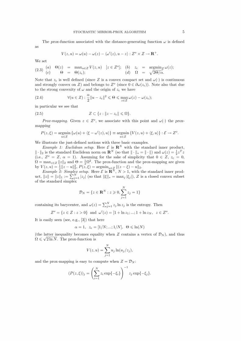
The prox-function associated with the distance-generating function ω is definedas

V (z, u) = ω(u)− ω(z)− 〈ω′(z), u− z〉 : Zo × Z → R+.

We set

(a) Θ(z) = maxu∈Z V (z, u) [z ∈ Zo]; (b) zc = argminZ ω(z);(c) Θ = Θ(zc); (d) Ω =

√2Θ/α.

(2.3)

Note that zc is well defined (since Z is a convex compact set and ω(·) is continuousand strongly convex on Z) and belongs to Zo (since 0 ∈ ∂ω(zc)). Note also that dueto the strong convexity of ω and the origin of zc we have

∀(u ∈ Z) :α

2‖u− zc‖2 6 Θ 6 max

z∈Zω(z)− ω(zc);(2.4)

in particular we see that

Z ⊂ z : ‖z − zc‖ 6 Ω.(2.5)

Prox-mapping. Given z ∈ Zo, we associate with this point and ω(·) the prox-mapping

P (z, ξ) = argminu∈Z

ω(u) + 〈ξ − ω′(z), u〉 ≡ argminu∈Z

V (z, u) + 〈ξ, u〉 : E → Zo.

We illustrate the just-defined notions with three basic examples.Example 1: Euclidean setup. Here E is RN with the standard inner product,

‖ · ‖2 is the standard Euclidean norm on RN (so that ‖ · ‖∗ = ‖ · ‖) and ω(z) = 12zT z

(i.e., Zo = Z, α = 1). Assuming for the sake of simplicity that 0 ∈ Z, zc = 0,Ω = maxz∈Z ‖z‖2 and Θ = 1

2Ω2. The prox-function and the prox-mapping are givenby V (z, u) = 1

2‖z − u‖22, P (z, ξ) = argminu∈Z ‖(z − ξ)− u‖2.Example 2: Simplex setup. Here E is RN , N > 1, with the standard inner prod-

uct, ‖z‖ = ‖z‖1 :=∑N

j=1 |zj | (so that ‖ξ‖∗ = maxj |ξj |), Z is a closed convex subsetof the standard simplex

DN = z ∈ RN : z > 0,

N∑

j=1

zj = 1

containing its barycenter, and ω(z) =∑N

j=1 zj ln zj is the entropy. Then

Zo = z ∈ Z : z > 0 and ω′(z) = [1 + ln z1; ...; 1 + ln zN , z ∈ Zo.

It is easily seen (see, e.g., [3]) that here

α = 1, zc = [1/N ; ...; 1/N ], Θ 6 ln(N)

(the latter inequality becomes equality when Z contains a vertex of DN ), and thusΩ 6

√2 ln N . The prox-function is

V (z, u) =N∑

j=1

uj ln(uj/zj),

and the prox-mapping is easy to compute when Z = DN :

(P (z, ξ))j =

(N∑

i=1

zi exp−ξi)−1

zj exp−ξj.


Example 3: Spectahedron setup. This is the “matrix analogy” of the Simplexsetup. Specifically, now E is the space of N ×N block-diagonal symmetric matrices,N > 1, of a given block-diagonal structure equipped with the Frobenius inner product〈a, b〉F = Tr(ab) and the trace norm |a|1 =

∑Ni=1 |λi(a)|, where λ1(a) > ... > λN (a)

are the eigenvalues of a symmetric N ×N matrix a; the conjugate norm |a|∞ is theusual spectral norm (the largest singular value) of a. Z is assumed to be a closedconvex subset of the spectahedron S = z ∈ E : z º 0, Tr(z) = 1 containing thematrix N−1IN . The distance-generating function is the matrix entropy

ω(z) =N∑

j=1

λj(z) ln λj(z),

so that Zo = z ∈ Z : z Â 0 and Ω′(z) = ln(z). This setup, similarly to the Simplexone, results in α = 1, zc = N−1IN , Θ = lnN and Ω =

√2 ln N [2]. When Z = S,

it is relatively easy to compute the prox-mapping (see [2, 7]); this task reduces tothe singular value decomposition of a matrix from E . It should be added that thematrices from S are exactly the matrices of the form

a = H(b) ≡ (Tr(expb))−1 expbwith b ∈ E . Note also that when Z = S, the prox-mapping becomes “linear in matrixlogarithm”: if z = H(a), then P (z, ξ) = H(a− ξ).

3. Stochastic Mirror-Prox algorithm.

3.1. Mirror-Prox algorithm with erroneous information. We are about topresent the Mirror-Prox algorithm proposed in [7]. In contrast to the original versionof the method, below we allow for errors when computing the values of F – we assumethat given a point z ∈ Z, we can compute an approximation F (z) ∈ E of F (z). Thet-step Mirror-Prox algorithm as applied to (1.2) is as follows:

Algorithm 3.1.1. Initialization: Choose r0 ∈ Zo and stepsizes γτ > 0, 1 6 τ 6 t.2. Step τ , τ = 1, 2, ..., t: Given rτ−1 ∈ Zo, set

wτ = P (rτ−1, γτ F (rτ−1)),rτ = P (rτ−1, γτ F (wτ ))

(3.1)

. When τ < t, loop to step t + 1.3. At step t, output

zt =

[t∑

τ=1

γτ

]−1 t∑τ=1

γτwτ .(3.2)

The preliminary technical result on the outlined algorithm is as follows.Theorem 3.2. Consider t-step algorithm 3.1 as applied to a v.i. (1.2) with a

monotone operator F satisfying (1.4). For τ = 1, 2, ..., let us set

∆τ = F (wτ )− F (wτ );

for z belonging to the trajectory r0, w1, r1, ..., wt, rt of the algorithm, let

εz = ‖F (z)− F (z)‖∗,


and let yτ ∈ Zotτ=0 be the sequence given by the recurrence

yτ = P (yτ−1, γτ∆τ ), y0 = r0.(3.3)

Assume that

γτ 6 α√3L

,(3.4)

Then

Errvi(zt) 6(

t∑τ=1

γτ

)−1

Γ(t),(3.5)

where Errvi(zt) is defined in (1.3),

Γ(t) = 2Θ(r0) +t∑

τ=1

3γ2τ

2α

[M2 + (εrτ−1 + εwτ )2 +

ε2wτ

3

](3.6)

+t∑

τ=1

〈γτ∆τ , wτ − yτ−1〉

and Θ(·) is defined by (2.3).Finally, when (1.2) is a Nash v.i., one can replace Errvi(zt) in (3.5) with ErrN(zt).

3.2. Main result. From now on, we focus on the case when Algorithm 3.1 solvesmonotone v.i. (1.2), and the corresponding monotone operator F is represented bya stochastic oracle. Specifically, at the i-th call to the SO, the input being z ∈ Z,the oracle returns the vector F = Ξ(z, ζi),, where ζi ∈ RN∞i=1 is a sequence ofi.i.d. random variables, and Ξ(z, ζ) : Z × RN → E is a Borel function. We referto this specific implementation of Algorithm 3.1 as to Stocastic Mirror Prox (SMP)algorithm.

In the sequel, we impose on the SO in question the following assumption, slightlymilder than (1.6):

Assumption I: With some µ ∈ [0,∞), for all z ∈ Z we have

(a) ‖E Ξ(z, ζi)− F (z) ‖∗ 6 µ(b) E

‖Ξ(z, ζi)− F (z)‖2∗

6 σ2.(3.7)

In some cases, we augment Assumption I by the followingAssumption II: For all z ∈ Z and all i we have

Eexp‖Ξ(z, ζi)− F (z)‖2∗/σ2 6 exp1.(3.8)

Note that Assumption II implies (3.7.b), since

expE‖Ξ(z, ζi)− F (z)‖2∗/σ2 6 E

exp‖Ξ(z, ζi)− F (z)‖2∗/σ2

by the Jensen inequality.From now on, assume that the starting point r0 in Algorithm 3.1 is the minimizer

zc of ω(·) on Z. Further, to avoid unnecessarily complicated formulas (and with noharm to the efficiency estimates) we stick to the constant stepsize policy γτ ≡ γ,


1 6 τ 6 t, where t is a fixed in advance number of iterations of the algorithm. Ourmain result is as follows:

Theorem 3.3. Let v.i. (1.2) with monotone operator F satisfying (1.4) be solvedby t-step Algorithm 3.1 using a SO, and let the stepsizes γτ ≡ γ, 1 6 τ 6 t, satisfy0 < γ 6 α√

3L. Then

(i) Under Assumption I, one has

EErrvi(zt)

6 K0(t) ≡

[αΩ2

tγ+

7γ

2α[M2 + 2σ2]

]+ 2µΩ,(3.9)

where M is the constant from (1.4) and Ω is given by (2.3).(ii) Under Assumptions I, II, one has, in addition to (3.9), for any Λ > 0,

ProbErrvi(zt) > K0(t) + ΛK1(t)

6 exp−Λ2/3+ exp−Λt,(3.10)

where

K1(t) =7σ2γ

2α+

2σΩ√t

.

In the case of a Nash v.i., Errvi(·) in (3.9), (3.10) can be replaced with ErrN(·).When optimizing the bound (3.9) in γ, we get the followingCorollary 3.4. In the situation of Theorem 3.3, let the stepsizes γτ ≡ γ be

chosen according to

γ = min

[α√3L

,αΩ

√2

7t(M2 + 2σ2)

].(3.11)

Then under Assumption I one has

EErrvi(zt

6 K∗

0 (t) ≡ max[

74

Ω2Lt + 7Ω

√M2+2σ2

3t

]+ 2µΩ, .(3.12)

(see (2.3)). Under Assumptions I, II, one has, in addition to (3.12), for any Λ > 0,

ProbErrvi(zt) > K∗

0 (t) + ΛK∗1 (t)

6 exp−Λ2/3+ exp−Λt(3.13)

with

K∗1 (t) =

72

Ωσ√t.(3.14)

In the case of a Nash v.i., Errvi(·) in (3.12), (3.13) can be replaced with ErrN(·).Remark 3.5. Observe that the upper bound (3.12) for the error of Algorithm 3.1

with stepsize strategy (3.11), in agreement with the lower bound of [6], depends in thesame way on the “size” σ of the perturbation Ξ(z, ζi)−F (z) and on the bound M forthe non-Lipschitz component of F . From now on to simplify the presentation, withslight abuse of notations, we denote M the maximum of these quantities. Clearly, thelatter implies that the bounds (3.7,b) and (3.8), and thus the bounds (3.12) – (3.14)of Corollary 3.4 hold with M substituted for σ.


3.3. Comparison with Robust Mirror SA Algorithm. Consider the caseof a Nash s.v.i. with operator F satisfying (1.4) with L = 0, and let the SO beunbiased (i.e., µ = 0). In this case, the bound (3.12) reads

E ErrN(zt 6 7ΩM√t

,(3.15)

where

M2 = max[

supz,z′∈Z

‖F (z)− F (z′)‖2∗, supz∈Z

E‖Ξ(z, ζi)− F (z)‖2∗

]

The bound (3.15) looks very much like the efficiency estimate

E ErrN(zt) 6 O(1)ΩM√

t(3.16)

(from now on, all O(1)’s are appropriate absolute positive constants) for the approx-imate solution zt of the t-step Robust Mirror SA (RMSA) algorithm [3]1). In thelatter estimate, Ω is exactly the same as in (3.15), and M is given by

M2

= max[sup

z‖F (z)‖2∗; sup

z∈ZE

‖Ξ(z, ζi)− F (z)‖2∗]

.

Note that we always have M 6 2M , and typically M and M are of the same order ofmagnitude; it may happen, however (think of the case when F is “almost constant”),that M ¿ M . Thus, the bound (3.15) never is worse, and sometimes can be muchbetter than the SA bound (3.16). It should be added that as far as implementationis concerned, the SMP algorithm is not more complicated than the RMSA (cf. thedescription of Algorithm 3.1 with the description

rt = P (rt−1, F (rt−1)),

zt =

[t∑

τ=1

γτ

]−1 t∑τ=1

γτrτ ,

of the RMSA).The just outlined advantage of SMP as compared to the usual Stochastic Ap-

proximation is not that important, since “typically” M and M are of the same order.We believe that the most interesting feature of the SMP algorithm is its ability totake advantage of a specific structure of a stochastic optimization problem, namely,insensitivity to the presence in the objective of large, but smooth and well-observablecomponents.

We are about to consider several less straightforward applications of the out-lined insensitivity of the SMP algorithm to smooth well-observed components in theobjective.

4. Application to Stochastic Approximation: Stochastic composite mi-nimization.

1) In this reference, only the Minimization and the Saddle Point problems are considered. How-ever, the results of [3] can be easily extended to s.v.i.’s.


4.1. Problem description. Consider the optimization problem as follows (cf.[6]):

minx∈X

φ(x) := Φ(φ1(x), ..., φm(x)),(4.1)

where1. X ⊂ X is a convex compact; the embedding space X is equipped with a

norm ‖ · ‖x, and X – with a distance-generating function ωx(x) with certainparameters αx,Θx, Ωx w.r.t. the norm ‖ · ‖x;

2. φ`(x) : X → E`, 1 6 ` 6 m, are Lipschitz continuous mappings taking valuesin Euclidean spaces E` equipped with norms (not necessarily the Euclideanones) ‖ · ‖(`) with conjugates ‖ · ‖(`,∗) and with closed convex cones K`. Wesuppose that φ` are K`-convex, i.e. for any x, x′ ∈ X, λ ∈ [0, 1],

φ`(λx + (1− λ)x′) 6K`λφ`(x) + (1− λ)φ`(x′),

where the notation a 6K b ⇔ b >K a means that b− a ∈ K.In addition to these structural restrictions, we assume that for all v, v′ ∈X, h ∈ X ,

(a) ‖[φ′`(v)− φ′`(v′)]h‖(`) 6 [Lx‖v − v′‖x + Mx]‖h‖x

(b) ‖[φ′`(v)]h‖(`) 6 [LxΩx + Mx]‖h‖x(4.2)

for certain selections φ′`(x) ∈ ∂K`φ`(x), x ∈ X2) and certain nonnegativeconstants Lx and Mx.

3. Functions φ`(·) are represented by an unbiased SO. At i-th call to the oracle,x ∈ X being the input, the oracle returns vectors f`(x, ζi) ∈ E` and linearmappings G`(x, ζi) from X to E`, 1 6 ` 6 m (ζi are i.i.d. random vectors)such that for any x ∈ X and i = 1, 2, ...,

(a) E f`(x, ζi) = φ`(x), 1 6 ` 6 m

(b) E

max16`6m

‖f`(x, ζi)− φ`(x)‖2(`)

6 M2xΩ2

x;

(c) E G`(x, ζi) = φ′`(x), 1 6 ` 6 m,

(d) E

maxh∈X‖h‖x61

‖[G`(x, ζi)− φ′`(x)]h‖2(`)

6 M2x , 1 6 ` 6 m.

(4.3)

4. Φ(·) is a convex function on E = E1 × ...× Em given by the representation

Φ(u1, ..., um) = maxy∈Y

m∑

`=1

〈u`,A`y + b`〉E`− Φ∗(y)

(4.4)

for u` ∈ E`, 1 6 ` 6 m. Here(a) Y ⊂ Y is a convex compact set containing the origin; the embedding

Euclidean space Y is equipped with a norm ‖·‖y, and Y - with a distance-generating function ωy(y) with parameters αy, Θy,Ωy w.r.t. the norm‖ · ‖y;

2) For a K-convex function φ : X → E (X ⊂ X is convex, K ⊂ E is a closed convex cone) andx ∈ X, the K-subdifferential ∂Kφ(x) is comprised of all linear mappings h 7→ Ph : X → E such thatφ(u) >K φ(x) + P(u − x) for all u ∈ X. When φ is Lipschitz continuous on X, ∂Kφ(x) 6= ∅ forall x ∈ X; if φ is differentiable at x ∈ int X (as it is the case almost everywhere on int X), one has∂φ(x)

∂x∈ ∂Kφ(x).


(b) The affine mappings y 7→ A`y+b` : Y → E` are such that A`y+b` ∈ K∗`

for all y ∈ Y and all `; here K∗` is the cone dual to K`;

(c) Φ∗(y) is a given convex function on Y such that

‖Φ′∗(y)− Φ′∗(y′)‖y,∗ 6 Ly‖y − y′‖y + My(4.5)

for certain selection Φ′∗(z) ∈ ∂Φ∗(y), y ∈ Y .Example: Stochastic Matrix Minimax problem (SMMP). For 1 6 ` 6 m, let E` = Sp`

be the space of symmetric p`×p` matrices equipped with the Frobenius inner product〈A,B〉F = Tr(AB) and the spectral norms | · |∞, and let K` be the cone Sp`

+ ofsymmetric positive semidefinite p` × p` matrices. Consider the problem

minx∈X

max16j6k

λmax

(m∑

`=1

PTj`φ`(x)Pj`

), (P )

where Pj` are given p` × qj matrices, and λmax(A) is the maximal eigenvalue of asymmetric matrix A. Observing that for a symmetric q × q matrix A one has

λmax(A) = maxS∈Sq

Tr(AS)

where Sq = S ∈ Sq+ : Tr(S) = 1. When denoting by Y the set of all symmetric

positive semidefinite block-diagonal matrices y = Diagy1, ..., yk with unit trace anddiagonal blocks yj of sizes qj × qj , we can represent (P ) in the form of (4.1), (4.4)with

Φ(u) := max16j6k

λmax

(m∑

`=1

Pj`u`PTj`

)

= maxy=Diagy1,...,yk∈Y

k∑

j=1

Tr

(m∑

`=1

PTj`u`Pj`yk

)


m∑

`=1

Tr

u`

k∑

j=1

PTj`ykPj`


m∑

`=1

〈u`,A`y〉F

(we put A`y =∑k

j=1 PTj`yjPj`). The set Y is the spectahedron in the space Sq of

symmetric block-diagonal matrices with k diagonal blocks of the sizes qj×qj , 1 6 j 6k. When equipping Y with the spectahedron setup, we get αy = 1, Θy = ln(

∑kj=1 qj)

and Ωy =√

2 ln(∑k

j=1 qj), see Section 2.2.Observe that in the simplest case of k = m, pj = qj , 1 6 j 6 m and Pj` equal to

Ip for j = ` and to 0 otherwise, the SMMP problem becomes

minx∈X

[max

16`6mλmax(φ`(x))

].(4.6)

If, in addition, pj = qj = 1 for all j, we arrive at the usual (“scalar”) minimax problem

minx∈X

[max

16`6mφ`(x)

](4.7)


with convex real-valued functions φ`.Observe that in the case of (4.4), the optimization problem (4.1) is nothing but

the primal problem associated with the saddle point problem

minx∈X

maxy∈Y

[φ(x, y) =

m∑

`=1

〈φ`(x),A`y + b`〉E`− Φ∗(y)

](4.8)

and the cost function in the latter problem is Lipschitz continuous and convex-concavedue to the K`-convexity of φ`(·) and the condition A`y + b` ∈ K∗

` whenever y ∈ Y .The associated Nash v.i. is given by the domain Z and the monotone mapping

F (z) ≡ F (x, y) =

[m∑

`=1

[φ′`(x)]∗[A`y + b`]; −m∑

`=1

A∗`φ`(x) + Φ′∗(y)

].(4.9)

The advantage of the v.i. reformulation of (4.1) is that F is linear in φ`(·), so thatthe initial unbiased SO for φ` induces an unbiased stochastic oracle for F , specifically,the oracle

Ξ(x, y, ζi) =

[m∑

`=1

G∗` (x, ζi)[A`y + b`]; −

m∑

`=1

A∗`f`(x, ζi) + Φ′∗(y)

].(4.10)

We are about to use this oracle in order to solve the stochastic composite minimizationproblem (4.1) by the SMP algorithm.

4.2. Setup for the SMP as applied to (4.9). In retrospect, the setup for SMPwe are about to present is a kind of the best – resulting in the best possible efficiencyestimate (3.12) – we can build from the entities participating in the description of theproblem (4.1). Specifically, we equip the space E = X × Y with the norm

‖[(x, y)‖ ≡√‖x‖2x/Ω2

x + ‖y‖2y/Ω2y;

the conjugate norm clearly is

‖(ξ, η)‖∗ =√

Ω2x‖ξ‖2x,∗ + Ω2

y‖η‖2y,∗.

Finally, we equip Z = X × Y with the distance-generating function

ω(x, y) =1

αxΩ2x

ωx(x) +1

αyΩ2y

ωy(y).

The SMP-related properties of our setup are summarized in the followingLemma 4.1. Let

A = maxy∈Y:‖y‖y61

m∑

`=1

‖A`y‖(`,∗), B =m∑

`=1

‖b`‖(`,∗).(4.11)

(i) The parameters of the just defined distance-generating function ω w.r.t. thejust defined norm ‖ · ‖ are α = 1, Θ = 1, Ω =

√2.

(ii) One has

∀(z, z′ ∈ Z) : ‖F (z)− F (z′)‖∗ 6 L‖z − z′‖+ M,(4.12)


where

L = 5AΩxΩy [ΩxLx + Mx] + BΩ2xLx + Ω2

yLy

M = [2AΩy + ‖b‖1] ΩxMx + ΩyMy

Besides this,

∀(z ∈ Z, i) : E Ξ(z, ζi) = F (z); E‖Ξ(z, ζi)− F (z)‖2∗

6 M2.(4.13)

Furethermore, if relations (4.3.b,d) are strengthened to

E

exp

max16`6m

‖f`(x, ζi)− φ`(x)‖2(`)/(ΩxM)2

6 exp1,

E

exp

maxh∈X ,‖h‖x61

‖[G`(x)− φ′`(x)]h‖2(`)/M2

6 exp1, 1 6 ` 6 m,

(4.14)

then

Eexp‖Ξ(z, ζi)− F (z)‖2∗/M2 6 exp1.(4.15)

Combining Lemma 4.1 with Corollary (3.4) we get explicit efficiency estimates for theSMP algorithm as applied to the Stochastic composite minimization problem (4.1).

4.3. Application to Stochastic Semidefinite Feasibility problem. Assumewe are interested to solve a feasible system of matrix inequalities

ψ`(x) ¹ 0, ` = 1, ..., m & x ∈ X,(4.16)

where m > 1, X ⊂ X is as in the description of the Stochastic composite problem,and ψ`(·) take values in the spaces E` = Sp` of symmetric p` × p` matrices. We equipE` with the Frobenius inner product, the semidefinite cone K` = Sp`

+ and the spectralnorm ‖ · ‖(`) = | · |∞ (recall that |A|∞ is the maximal singular value of matrix A). Weassume that ψ` are Lipschitz continuous and K` = Sp`

+ -convex functions on X suchthat for all x, x′ ∈ X and for all ` one has

maxh∈X , ‖h‖x61

|[ψ′`(x)− ψ′`(x′)]h|∞ 6 L`‖x− x′‖x + M`,


|ψ′`(x)h|∞ 6 L`Ωx + M`(4.17)

for certain selections ψ′`(x) ∈ ∂K`ψ`(x), x ∈ X, with some known nonnegative con-stants L`, M`.

We assume that ψ`(·) are represented by an SO which at i-th call, the input beingx ∈ X, returns the matrices f`(x, ζi) ∈ Sp` and the linear maps G`(x, ζi) from X toE` such that for all x ∈ X it holds

(a) E

f`(x, ζi)

= ψ`(x), EG`(x, ζi)

= ψ′`(x), 1 6 ` 6 m

(b) E

max16`6m

|f`(x, ζi)− ψ`(x)|2∞/(ΩxM`)2

6 1

(c) E

maxh∈X ,‖h‖x61

|[G`(x, ζi)− ψ′`(x)]h|2∞/M2`

6 1, 1 6 ` 6 m.

(4.18)

Given a number t of steps of the SMP algorithm, let us act as follows.


A. We compute the m quantities µ` = ΩxL`√t

+ M`, ` = 1, ..., m, and set

µ = max16`6m

µ`, β` =µ

µ`, φ`(·) = β`ψ`(·), Lx =

µ√

t

Ωx, Mx = µ.(4.19)

Note that by construction β` > 1 and Lx/L` > β`, Mx/M` > β` for all `, so that thefunctions φ` satisfy (4.2) with the just defined Lx, Mx. Further, the SO for ψ`(·)’scan be converted into an SO for φ`(·)’s by setting

f`(x, ζ) = β`f`(x, ζ), G`(x, ζ) = β`G`(x, ζ).

By (4.18), this oracle satisfies (4.3).B. We then build the Stochastic Matrix Minimax problem

minx∈X

max16`6m

λmax(φi(x)),(4.20)

associated with the just defined φ1, ..., φm, that is, the Stochastic composite problem(4.1) associated with φ1, ..., φm and the outer function

Φ(u1, ..., um) = max16`6m

λmax(u`) = maxy∈Y

m∑

`=1

〈u`, y`〉F ,

Y = y = Diagy1, ..., ym ∈ Y = Sp1 × ...× Spm : y º 0, Tr(y) = 1⊂ Y = Sp1 × ...× Spm .

Thus in the notation from (4.4) we have A`y = y`, b` = 0, Φ∗ ≡ 0. Hence Lx = Mx =0, and Y is a spectahedron. We equip Y and Y with the Spectahedron setup, arrivingat

αy = 1, Θy = lnm∑

`=1

p`, Ωy =

√√√√2 lnm∑

`=1

p`.

C. We have specified all entities participating in the description of the Stochasticcomposite problem. It is immediately seen that these entities satisfy all conditionsof Section 4.1. We can now solve the resulting Stochastic composite problem byt-step SMP algorithm with the setup presented in Section 4.2. The correspondingconvex-concave saddle point problem is

minx∈X

maxy∈Y

m∑

`=1

β`〈ψ`(x), y`〉F ;

with the monotone operator and SO, respectively,

F (z) ≡ F (x, y) =

[m∑

`=1

β`[ψ′`(x)]∗y`;−Diag α1ψ1(x), ..., αmψm(x)]

,

Ξ((x, y), ζ) =

[m∑

`=1

β`G∗` (x, ζ)y`;−Diag

α1f1(x, ζ), ..., αmfm(x, ζ))

].

Combining Lemma 4.1, Corollary 3.4 and taking into account the origin of the quan-tities Lx, Mx, and the fact that A = 1, B = 0 3), we arrive at the following result:

3) See (4.11) and note that we are in the case when b` = 0 and ‖ · ‖(`,∗) is the trace norm; thus,∑m`=1 ‖A`y‖(`,∗) =

∑m`=1 |y`|1 = |y|1 = ‖y‖y.


Proposition 4.2. With the outlined construction, the resulting s.v.i. reads

find z∗ ∈ Z = X × Y : 〈F (z), z − z∗〉 > 0 ∀z ∈ Z,(4.21)

for the monotone operator F which satisfies (1.4) with

L = 10

[ln

m∑

`=1

p`

] 12

Ωxµ(√

t + 1), M = 4

[ln

m∑

`=1

p`

] 12

Ωxµ;

Beside this, the resulting SO for F satisfies (4.13) with the just defined value of M .Let now

γ =

10

[3 ln

m∑

`=1

p`

] 12

Ωxµ(√

t + 1)

−1

, 1 6 τ 6 t.

When applying to (4.21) the t-step SMP algorithm with the constant stepsizes γτ ≡ γ(cf. (3.11) and note that we are in the situation α = Θ = 1), we get an approximatesolution zt = (xt, yt) such that

E

max16`6m

β`λmax(ψ`(xt))

6 80Ωx [ln

∑m`=1 p`]

12 µ√

t(4.22)

(cf. (3.12) and take into account that we are in the case of Ω =√

2, while the optimalvalue in (4.20) is nonpositive, since (4.16) is feasible).

Furthermore, if assumptions (4.18.b,c) are strengthened to

E

max16`6m

exp|f`(x, ζi)− ψ`(x)|2∞/(ΩxM`)2

6 exp1,

E

exp maxh∈X , ‖h‖x61

|[G`(x, ζi)− ψ′`(x)]h|2∞/M2`

6 exp1, 1 6 ` 6 m,

then, in addition to (4.22), we have for any Λ > 0:

Prob

max

16`6mβ`λmax(ψ`(xt)) > 80

[ln(∑m

`=1 p`)]12 Ωxµ√

t+ Λ

15 [ln∑m

`=1 p`]12 Ωxµ√

t

6 exp−Λ2/3+ exp−Λt.

Discussion. Imagine that instead of solving the system of matrix inequalities(4.16), we were interested to solve just a single matrix inequality ψ`(x) ¹ 0, x ∈ X.When solving this inequality by the SMP algorithm as explained above, the efficiencyestimate would be

Eψ`(x`

t)

6 O(1) [ln(p` + 1)]1/2 Ωx

[ΩxL`

t+

M`√t

]= O(1) [ln(p` + 1)]1/2 Ωx

µ`√t

= O(1) [ln(p` + 1)]1/2β−1

`

Ωxµ√t

,


(recall that the matrix inequality in question is feasible), where x`t is the resulting

approximate solution. Looking at (4.22), we see that the expected accuracy of theSMP as applied, in the aforementioned manner, to (4.16) is only by a logarithmic in∑

` p` factor worse:

E ψ`(xt) 6 O(1)

[ln

m∑

`=1

p`

]1/2

β−1`

Ωxµ√t

= O(1)

[ln

m∑

`=1

p`

]1/2Ωxµ`√

t.(4.23)

Thus, as far as the quality of the SPM-generated solution is concerned, passing fromsolving a single matrix inequality to solving a system of m inequalities is “nearlycostless”. As an illustration, consider the case where some of ψ` are “easy” – smoothand easy-to-observe (M` = 0), while the remaining ψ` are “difficult”, i.e., might benon-smooth and/or difficult-to-observe (L` = 0). In this case, (4.23) reads

E ψ`(xt) 6

O(1) [ln∑m

`=1 p`]1/2 Ω2

xL`

t , ψ` is easy,

O(1) [ln∑m

`=1 p`]1/2 ΩxM`√

t, ψ` is difficult.

In other words, the violations of the easy and the difficult constraints in (4.16) convergeto 0 as t → ∞ with the rates O(1/t) and O(1/

√t), respectively. It should be added

that when X is the unit Euclidean ball in X = Rn and X, X are equipped with theEuclidean setup, the rates of convergence O(1/t) and O(1/

√t) are the best rates one

can achieve without imposing bounds on n and/or imposing additional restrictionson ψ`’s.

4.4. Eigenvalue optimization via SMP. The problem we are interested innow is

Opt = minx∈X

f(x) := λmax(A0 + x1A1 + ... + xnAn),

X = x ∈ Rn : x > 0,∑n

i=1 xi = 1,(4.24)

where A0, A1, ..., An, n > 1, are given symmetric matrices with common block-diagonal structure (p1, ..., pm). I.e., all Aj are block-diagonal with diagonal blocksA`

j of sizes p` × p`, 1 6 ` 6 m. We denote

p(κ) =m∑

`=1

pκ` , κ = 1, 2, 3; pmax = max

`p`; A∞ = max

16j6n|Aj |∞.

Setting

φ` : X 7→ E` = Sp` , φ`(x) = A`0 +

n∑

j=1

xjA`j , 1 6 ` 6 m,

we represent (4.24) as a particular case of the Matrix Minimax problem (4.6), withall functions φ`(x) being affine and X being the standard simplex in X = Rn.

Now, since Aj are known in advance, there is nothing stochastic in our problem,and it can be solved either by interior point methods, or by “computationally cheap”gradient-type methods; these latter methods are preferable when the problem is large-scale and medium accuracy solutions are sought. For instance, one can apply the t-step


(deterministic) Mirror Prox algorithm DMP from [7] to the saddle point reformulation(4.8) of our specific Matrix Minimax problem, i.e., to the saddle point problem

minx∈X

maxy∈Y

〈y, A0 +∑n

j=1 xjAj〉F ,

Y =y = Diagy1, ..., ym : y` ∈ Sp`

+ , 1 6 ` 6 m, Tr(Y ) = 1

.(4.25)

The accuracy of the approximate solution xt of the DMP algorithm is [7, Example 2]

f(xt)−Opt 6 O(1)

√ln(n) ln(p(1))A∞

t.(4.26)

This efficiency estimate is the best known so far among those attainable with “com-putationally cheap” deterministic methods. On the other hand, the complexity ofone step of the algorithm is dominated, up to an absolute constant factor, by thenecessity, given x ∈ X and y ∈ Y ,

1. to compute the matrix A0+∑n

j=1 xjAj and the vector [Tr(Y A1); ...; Tr(Y An)];2. to compute the eigenvalue decomposition of y.

When using the standard Linear Algebra, the computational effort per step is

Cdet = O(1)[np(2) + p(3)](4.27)

arithmetic operations.We are about to demonstrate that one can equip the deterministic problem in

question by an “artificial” SO in such a way that the associated SMP algorithm, undercertain circumstances, exhibits better performance than deterministic algorithms. Letus consider the following construction of the SO for F (different from the SO (4.10)!).Observe that the monotone operator associated with the saddle point problem (4.25)is

F (x, y) =[

[Tr(yA1); ...; Tr(yAn)]︸︷︷︸F x(x,y)

; −A0 −∑n

j=1xjAj

︸︷︷︸F y(x,y)

].(4.28)

Given x ∈ X, y = Diagy1, ..., ym ∈ Y , we build a random estimate Ξ = [Ξx; Ξy] ofF (x, y) = [F x(x, y); F y(x, y)] as follows:

1. we generate a realization of a random variable taking values 1, ..., n withprobabilities x1, ..., xn (recall that x ∈ X, the standard simplex, so that xindeed can be seen as a probability distribution), and set

Ξy = A0 + A;(4.29)

2. we compute the quantities ν` = Tr(y`), 1 6 ` 6 m. Since y ∈ Y , we haveν` > 0 and

∑m`=1 ν` = 1. We further generate a realization ı of random

variable taking values 1, ...,m with probabilities ν1, ..., νm, and set

Ξx = [Tr(Aı1yı); ...; Tr(Aı

nyı)], yı = (Tr(yı))−1yı.(4.30)

The just defined random estimate Ξ of F (x, y) can be expressed as a deterministicfunction Ξ(x, y, η) of (x, y) and random variable η uniformly distributed on [0, 1].Assuming all matrices Aj directly available (so that it takes O(1) arithmetic operationsto extract a particular entry of Aj given j and indexes of the entry) and given x, y andη, the value Ξ(x, y, ξ) can be computed with the arithmetic cost O(1)(n(pmax)2 +p(2))


(indeed, O(1)(n + p(1)) operations are needed to convert η into ı and , O(1)p(2)

operations are used to write down the y-component −A0−A of Ξ, and O(1)n(pmax)2

operations are needed to compute Ξx). Now consider the SO’s Ξk (k is a positiveinteger) obtained by averaging the outputs of k calls to our basic oracle Ξ. Specifically,at the i-t call to the oracle Ξk, z = (x, y) ∈ Z = X × Y being the input, the oraclereturns the vector

Ξk(z, ζi) =1k

k∑s=1

Ξ(z, ηis),

where ζi = [ηi1; ...; ηik] and ηis16i, 16s6k are independent random variables uni-formly distributed on [0, 1]. Note that the arithmetic cost of a single call to Ξk is

Ck = O(1)k(n(pmax)2 + p(2)).

The Nash v.i. associated with the saddle point problem (4.25) with the stochasticoracle Ξk (k being the first parameter of our construction) specify a Nash s.v.i. onthe domain Z = X × Y . Let us equip the standard simplex X and its embeddingspace X = Rn with the Simplex setup, and the spectahedron Y and its embeddingspace Y = Sp1 × ...×Spm with the Spectahedron setup (see Section 2.2). Let us nextcombine the x- and the y-setups, exactly as explained in the beginning of Section 4.2,into an SMP setup for the domain Z = X × Y – a distance-generating function ω(·)and a norm ‖ ·‖ on the embedding space Rn× (Sp1× ...×Sp`) of Z. The SMP-relatedproperties of the resulting setup are summarized in the following statement.

Lemma 4.3. Let n > 3, p(1) > 3. Then(i) The parameters of the just defined distance-generating function ω w.r.t. the

just defined norm ‖ · ‖ are α = 1, Θ = 1, Ω =√

2.(ii) For any z, z′ ∈ Z one has

‖F (z)− F (z′)‖∗ 6 L‖z − z′‖, L = 2[ln(n) + 2 ln(p(1))]A∞.(4.31)

Besides this, for any (z ∈ Z, i = 1, 2, ...,

(a) E Ξk(z, ζi) = F (z);(b) E

exp‖Ξ(z, ζi)− F (z)‖2∗/M2 6 exp1,

M = 27[ln(n) + ln(p(1))]A∞/√

k.(4.32)

Combining Lemma 4.3 and Corollary 3.4, we arrive at the followingProposition 4.4. With properly chosen positive absolute constants O(1), the

t-step SMP algorithm with constant stepsizes

γτ = O(1)min[1,

√k/t]

ln(np(1))A∞, 1 6 τ 6 t [A∞ = max

16j6n|Aj |∞]

as applied to the saddle point reformulation of problem (4.24), the stochastic oraclebeing Ξk, produces a random feasible approximate solution xt to the problem with theerror

ε(xt) = λmax

A0 +

n∑

j=1

[xt]jAj

−Opt


satisfying

E ε(xt) 6 O(1) ln(np(1))A∞[

1t + 1√

kt

],

∀Λ > 0 : Prob

ε(xt) > O(1) ln(np(1))A∞[

1t + [1 + Λ] 1√

kt

]

6 exp−Λ2/3+ exp−Λt(4.33)

Assuming all matrices Aj directly available, the overall computational effort to com-pute xt is

C = O(1)t[k(n(pmax)2 + p(2)) + p(3)

](4.34)

arithmetic operations, where O(1)k(n(pmax)2 + p(2)) operations per step is the priceof two calls to the stochastic oracle Ξk and O(1)(n + p(3)) operations per step is theprice of computing two prox mappings.

Discussion. Let us find out whether randomization can help when solving a large-scale problem(4.24), that is, whether, given quality of the resulting approximate solu-tion, the computational effort to build such a solution with the Stochastic Mirror Proxalgorithm SMP can be essentially less than the one for the deterministic Mirror Proxalgorithm DMP. To simplify our considerations, assume from now on that p` = p,1 6 ` 6 m, and that ln(n) = O(1) ln(mp). Assume also that we are interested in a(perhaps, random) solution xt which with probability > 1− δ satisfies ε(xt) 6 ε. Wefix the tolerance δ ¿ 1 and the relative accuracy ν = ε

ln(mnp)A∞6 1 and look what

happens when (some of) the sizes m,n, p of the problem become large.Observe first of all that the overall computational effort to solve (4.24) within

relative accuracy ν with the DMP algorithm is

CDMP(ν) = O(1)m(n + p)p2ν−1

operations (see (4.26), (4.27)). As about the SMP algorithm, let us choose k whichbalances the per step computational effort O(1)k(n(pmax)2 + p(2)) = O(1)k(n + m)p2

to produce the answers of the stochastic oracle and the per step cost of prox mappingsO(1)(n+mp3), that is, let us set k = Ceil

(mp

m+n

). With this choice of k, Proposition

4.4 says that to get a solution of the required quality, it suffices to carry out

t = O(1)[ν−1 + ln(1/δ)k−1ν−2

](4.35)

steps of the method, provided that this number of steps is >√

ln(2/δ). The latterassumption is automatically satisfied when the absolute constant factor in (4.35) is> 1 and ν

√ln(2/δ) 6 1, which we assume from now on. Combining (4.35) and the

upper bounds on the arithmetic cost of an SMP step stated in Proposition 4.4, weconclude that the overall computational effort to produce a solution of the requiredquality with the SMP algorithm is

CSMP(ν, δ) = O(1)k(n + m)p2[ν−1 + ln(1/δ)k−1ν−2

]

operations, so that

R :=CDMP(ν)CSMP(ν, δ)

= O(1)m(n + p)

(n + m)(k + ln(1/δ)ν−1)[k = Ceil

(mp

m+n

)]


We see that when ν, δ are fixed and both m n+pn+m and n/p are large, then R is large

as well, that is, the randomized algorithm outperforms significantly its deterministiccounterpart.

Another interesting observation is as follows. In order to produce, with probability> 1− δ, an approximate solution to (4.24) with relative accuracy ν, the just definedSMP algorithm requires t steps, with t given by (4.35), and at every one of these stepsit “visits” O(1)k(m+n)p2 chosen at random entries in the data matrices A0, A1, ..., An.The overall number of data entries visited by the algorithm is therefore NSMP =O(1)tk(m + n)p2 = O(1)

[kν−1 + ln(1/δ)ν−2

](m + n)p2. At the same time, the total

number of data entries is N tot = m(n + 1)p2. Therefore

ϑ :=NSMP

N tot= O(1)

[kν−1 + ln(1/δ)ν−2

] [1m

+1n

][k = Ceil

(mp

m+n

)]

We see that when δ, ν are fixed and m, n and n/p are large, ϑ is small, i.e., theapproximate solution of the required quality is built when inspecting a tiny fractionof the data. This sublinear time behaviour [13] was already observed in [3] for theRobust Mirror Descent Stochastic Approximation as applied to a matrix game (thelatter problem is the particular case of (4.24) with p1 = ... = pm = 1 and A0 = 0).

REFERENCES

[1] Azuma, K. Weighted sums of certain dependent random variables. Tokuku Math. J., 19 (1967),357-367.

[2] Ben-Tal, A., Nemirovski, A. “Non-Euclidean restricted memory level method for large-scaleconvex optimization” – Math. Progr. 102 (2005), 407–456.

[3] Juditsky, A. Lan, G., Nemirovski, A., Shapiro, A., Stochastic Approximation Approach toStochastic Programming,http://www.optimization-online.org/DB HTML/2007/09/1787.html

[4] Juditsky, A., Nemirovski, A. (2008), Large Deviations of Vector-valued Martingales in 2-Smooth Normed SpacesE-print: http://www.optimization-online.org/DB HTML/2008/04/1947.html

[5] Korpelevich, G. “Extrapolation gradient methods and relation to Modified Lagrangeans”Ekonomika i Matematicheskie Metody, 19 (1983), 694-703 (in Russian; English trans-lation in Matekon).

[6] Nemirovski, A., Yudin, D., Problem complexity and method eciency in Optimization J. Wiley& Sons (1983).

[7] A. Nemirovski, “Prox-method with rate of convergence O(1/t) for variational inequalitieswith Lipschitz continuous monotone operators and smooth convex-concave saddle pointproblems” – SIAM J. Optim. 15 (2004), 229-251.

[8] Lu, Z., Nemirovski A., Monteiro, R. “Large-Scale Semidefinite Programming via Saddle PointMirror-Prox Algorithm”, Math. Progr., 109 (2007), 211-237.

[9] Nemirovski, A., Onn, S., Rothblum, U. (2007), “Accuracy certificates for computational prob-lems with convex structure” – submitted to Mathematics of Operations Research. E-print:http://www.optimization-online.org/DB HTML/2007/04/1634.html

[10] Nesterov, Yu. “Smooth minimization of non-smooth functions”, Math. Progr., 103 (2005),127-152.

[11] Nesterov, Yu. “Excessive gap technique in nonsmooth convex minimization”, SIAM J. Optim.,16 (2005), 235-249.

[12] Nesterov, Yu. “Dual extrapolation and its applications to solving variational inequalities andrelated problems”, Math. Progr. 109 (2007) 319-344.

[13] Rubinfeld, R., Sublinear time algorithms. – Marta Sanz-Sole, Javier Soria, Juan Luis Varona,Joan Verdera, Eds. International Congress of Mathematicians, Madrid 2006, Vol. III,1o95–11110. European Mathematical Society Publishing House, 2006.

5. Appendix.


5.1. Proof of Theorem 3.2. We start with the following simple observation:if re is a solution to (2.2), then ∂Zω(re) contains −e and thus is nonempty, so thatre ∈ Zo. Moreover, one has

〈ω′(re)− e, u− re〉 > 0 ∀u ∈ Z.(5.1)

Indeed, by continuity argument, it suffices to verify the inequality in the case whenu ∈ rint(Z) ⊂ Zo. For such an u, the convex function

f(t) = ω(re + t(u− re)) + 〈re + t(u− re), e〉, t ∈ [0, 1]

is continuous on [0, 1] and has a continuous on [0, 1] field of subgradients

g(t) = 〈ω′(re + t(u− re)) + e, u− re〉.

It follows that the function is continuously differentiable on [0, 1] with the derivativeg(t). Since the function attains its minimum on [0, 1] at t = 0, we have g(0) > 0,which is exactly (5.1).

At least the first statement of the following Lemma is well-known:Lemma 5.1. For every z ∈ Zo, the mapping ξ 7→ P (z, ξ) is a single-valued

mapping of E onto Zo, and this mapping is Lipschitz continuous, specifically,

‖P (z, ζ)− P (z, η)‖ 6 α−1‖ζ − η‖∗ ∀ζ, η ∈ E .(5.2)

Besides this,

(a) ∀(u ∈ Z) : V (P (z, ζ), u) 6 V (z, u) + 〈ζ, u− P (z, ζ)〉 − V (z, P (z, ζ))(b) 6 V (z, u) + 〈ζ, u− z〉+ ‖ζ‖2∗

2α .(5.3)

Proof.Let v ∈ P (z, ζ), w ∈ P (z, η). As V ′

u(z, u) = ω′(u) − ω′(z), invoking 5.1, we havev, w ∈ Zo and

〈ω′(v)− ω′(z) + ζ, v − u〉 6 0 ∀u ∈ Z.(5.4)

〈ω′(w)− ω′(z) + η, w − u〉 6 0 ∀u ∈ Z.(5.5)

Setting u = w in (5.4) and u = v in (5.5), we get

〈ω′(v)− ω′(z) + ζ, v − w〉 6 0, 〈ω′(w)− ω′(z) + η, v − w〉 > 0,

whence 〈ω′(w)− ω′(v) + [η − ζ], v − w〉 > 0, or

‖η − ζ‖∗‖v − w‖ > 〈η − ζ, v − w〉 > 〈ω′(v)− ω′(w), v − w〉 > α‖v − w‖2,

and (5.2) follows. This relation, as a byproduct, implies that P (z, ·) is single-valued.To prove (5.3), let v = P (z, ζ). We have

V (v, u)− V (z, u) = [ω(u)− 〈ω′(v), u− v〉 − ω(v)]− [ω(u)− 〈ω′(z), u− z〉 − ω(z)]= 〈ω′(v)− ω′(z) + ζ, v − u〉+ 〈ζ, u− v〉 − [ω(v)− 〈ω′(z), v − z〉 − ω(z)]

(due to (5.4)) 6 〈ζ, u− v〉 − V (z, v),


as required in (a) of (5.3). The bound (b) of (5.3) is obtained from (5.3) using theYoung inequality:

〈ζ, z − v〉 6 ‖z‖2∗2α

+α

2‖z − v‖2.

Indeed, observe that by definition, V (z, ·) is strongly convex with parameter α, andV (z, v) > α

2 ‖z − v‖2, so that

〈ζ, u− v〉 − V (z, v) = 〈ζ, u− z〉+ 〈ζ, z − v〉 − V (z, v) 6 〈ζ, u− z〉+‖ζ‖2∗2α

.

We have the following simple corollary of Lemma 5.1:Corollary 5.2. Let ξ1, ξ2, ... be a sequence of elements of E. Define the sequence

yτ∞τ=0 in Zo as follows:

yτ = P (yτ−1, ξτ ), y0 ∈ Zo.

Then yτ is a measurable function of y0 and ξ1, ..., ξτ such that

(∀u ∈ Z) : 〈−t∑

τ=1

ξτ , u〉 6 V (y0, u) +t∑

τ=1

ζτ ,(5.6)

with

|ζτ | 6 r‖ξτ‖∗ (here r = maxu∈Z

‖u‖); ζτ 6 −〈ξτ , yτ−1〉+‖ξτ‖2∗2α

.(5.7)

Proof. Using the bound (b) of (5.3) with ζ = ξt and z = yt−1 (so that yt =P (yt−1, ξt) we obtain for any u ∈ Z:

V (yt, u)− V (yt−1, u)− 〈ξt, u〉 6 −〈ξt, yt〉 − V (yt−1, yt) ≡ ζt.

Note that

ζt = maxv∈Z

[−〈ξt, v〉 − V (yt−1, v)],

so that

−r‖ξt‖∗ 6 −〈ξt, yt−1〉 6 ζt 6 r‖ξt‖∗.

Further, due to the strong convexity of V ,

ζt = −〈ξt, yt−1〉+ [−〈ξt, yt − yt−1〉 − V (yt−1, yt)] 6 −〈ξt, yt−1〉+‖ξt‖2∗2α

.

When summing up from τ = 1 to τ = t we arrive at the corollary.We also need the following result.Lemma 5.3. Let z ∈ Zo, let ζ, η be two points from E, and let

w = P (z, ζ), r+ = P (z, η)


Then for all u ∈ Z one has

(a) ‖w − r+‖ 6 α−1‖ζ − η‖∗(b) V (r+, u)− V (z, u) 6 〈η, u− w〉+ ‖ζ−η‖2∗

2α − α2 ‖w − z‖2.(5.8)

Proof. (a): this is nothing but (5.2).(b): Using (a) of (5.3) in Lemma 5.1 we can write for u = r+:

V (w, r+) 6 V (z, r+) + 〈ζ, r+ − w〉 − V (z, w).

This results in

V (z, r+) > V (w, r+) + V (z, w) + 〈ζ, w − r+〉.(5.9)

Using (5.3) with η substituted for ζ we get

V (r+, u) 6 V (z, u) + 〈η, u− r+〉 − V (z, r+)= V (z, u) + 〈η, u− w〉+ 〈η, w − r+〉 − V (z, r+)

[by (5.9)] 6 V (z, u) + 〈η, u− w〉+ 〈η − ζ, w − r+〉 − V (z, w)− V (w, r+)

6 V (z, u) + 〈η, u− w〉+ 〈η − ζ, w − r+〉 − α

2[‖w − z‖2 + ‖w − r+‖2],

due to the strong convexity of V . To conclude the bound (b) of (5.8) it suffices tonote that by the Young inequality,

〈η − ζ, w − r+〉 6 ‖η − ζ‖2∗2α

+α

2‖w − r+‖2.

We are able now to prove Theorem 3.2. By (1.4) we have that

‖F (wτ )− F (rτ−1)‖2∗ 6 (L‖rτ−1 − wτ‖+ M + εrτ−1 + εwτ )2

6 3L2‖wτ − rτ−1‖2 + 3M2 + 3(εrτ−1 + εwτ )2.(5.10)

Let us now apply Lemma 5.3 with z = rτ−1, ζ = γτ F (rτ−1), η = γτ F (wτ ) (so thatw = wτ and r+ = rτ ). We have for any u ∈ Z

〈γτ F (wτ ), wτ − u〉+ V (rτ , u)− V (rτ−1, u)

6 γ2τ

2α‖F (wτ )− F (rτ−1)‖2 − α

2‖wτ − rτ−1‖2

[by (5.10)] 6 3γ2τL2

2α

[‖wτ − rτ−1‖2 + M2 + (εrτ−1 + εwτ )2]− α

2‖wτ − rτ−1‖2

[by (3.4)] 6 3γ2τ

2α

[M2 + (εrτ−1 + εwτ )2

]

When summing up from τ = 1 to τ = t we obtain

t∑τ=1

〈γτ F (wτ ), wτ − u〉 6 V (r0, u)− V (rt, u) +t∑

τ=1

3γ2τ

2α

[M2 + (εrτ−1 + εwτ )2

]

6 Θ(r0) +t∑

τ=1

3γ2τ

2α

[M2 + (εrτ−1 + εwτ )2

].


Hence, for all u ∈ Z,

t∑τ=1

〈γτF (wτ ), wτ − u〉

6 Θ(r0) +t∑

τ=1

3γ2τ

2α

[M2 + (εrτ−1 + εwτ

)2]+

t∑τ=1

〈γτ∆τ , wτ − u〉

= Θ(r0) +t∑

τ=1

3γ2τ

2α

[M2 + (εrτ−1 + εwτ

)2]+

t∑τ=1

〈γτ∆τ , wτ − yτ−1〉(5.11)

+t∑

τ=1

〈γτ∆τ , yτ−1 − u〉,

where yτ are given by (3.3). Since the sequences yτ, ξτ = γτ∆τ satisfy thepremise of Corollary 5.2, we have

(∀u ∈ Z) :∑t

τ=1〈γτ∆τ , yτ−1 − u〉 6 V (r0, u) +∑t

τ=1γ2

τ

2α‖∆τ‖2∗6 Θ(r0) +

∑tτ=1

γ2τ

2αε2wτ,

and thus (5.11) implies that for any u ∈ Z

t∑τ=1

〈γτF (wτ ), wτ − u〉 6 2Θ(r0) +t∑

τ=1

〈γτ∆τ , wτ − yτ−1〉(5.12)

+t∑

τ=1

3γ2τ

2α

[M2 + (εrτ−1 + εwτ )2 +

ε2wτ

3

]

To complete the proof of (3.5) in the general case, note that since F is monotone,(5.12) implies that for all u ∈ Z,

t∑τ=1

γτ 〈F (u), wτ − u〉 6 Γ(t),

where

Γ(t) = 2Θ(r0) +t∑

τ=1

3γ2τ

2α

[M2 + (εrτ−1 + εwτ )2 +

ε2wτ

3

]+

t∑τ=1

〈γτ∆τ , wτ − yτ−1〉

(cf. (3.6)), whence

∀(u ∈ Z) : 〈F (u), zt − u〉 6[

t∑τ=1

γτ

]−1

Γ(t).

When taking the supremum over u ∈ Z, we arrive at (3.5).In the case of a Nash v.i., setting wτ = (wτ,1, ..., wτ,m) and u = (u1, ..., um) and

recalling the origin of F , due to the convexity of φi(zi, zi) in zi, for all u ∈ Z we get

from (5.12):

t∑τ=1

γτ

m∑

i=1

[φi(wτ )− φi(ui, (wτ )i)] 6t∑

τ=1

γτ

m∑

i=1

〈F i(wτ ), (wτ )i − ui〉 6 Γ(t).


Setting φ(z) =∑m

i=1 φi(z), we get

t∑τ=1

γτ

[φ(wτ )−

m∑

i=1

φi(ui, (wτ )i)

]6 Γ(t).

Recalling that φ(·) is convex and φi(ui, ·) are concave, i = 1, ...,m, the latter inequalityimplies that

[t∑

τ=1

γτ

][φ(zt)−

m∑

i=1

φi(ui, (zt)i)

]6 Γ(t),

or, which is the same,

m∑

i=1

[φi(zt)−

m∑

i=1

φi(ui, (zt)i)

]6

[t∑

τ=1

γτ

]−1

Γ(t).

This relation holds true for all u = (u1, ..., um) ∈ Z; taking maximum of both sidesin u, we get

ErrN(zt) 6[

t∑τ=1

γτ

]−1

Γ(t).

5.2. Proof of Theorem 3.3. In what follows, we use the notation from Theo-rem 3.2. By this theorem, in the case of constant stepsizes γτ ≡ γ we have

Errvi(zt) 6 [tγ]−1 Γ(t),(5.13)

where

Γ(t) = 2Θ +3γ2

2α

t∑τ=1

[M2 + (εrτ−1 + εwτ )2 +

ε2wτ

3

]+ γ

t∑τ=1

〈∆τ , wτ − yτ−1〉

6 2Θ +7γ2

2α

t∑τ=1

[M2 + ε2rτ−1

+ ε2wτ

]+ γ

t∑τ=1

〈∆τ , wτ − yτ−1〉.(5.14)

For a Nash v.i., Errvi in this relation can be replaced with ErrN.Note that by description of the algorithm rτ−1 is a deterministic function of

ζN(τ−1) and wτ is a deterministic function of ζM(τ) for certain increasing sequencesof integers M(τ), N(τ) such that N(τ − 1) < M(τ) < N(τ). Therefore εrτ−1 isa deterministic function of ζN(τ−1)+1, and εwτ and ∆τ are deterministic functions ofζM(τ)+1. Denoting by Ei the expectation w.r.t. ζi, we conclude that under assumptionI we have

EN(τ−1)+1

ε2rτ−1

6 σ2, EM(τ)+1

ε2wτ

6 σ2, ‖EM(τ)+1 ∆τ ‖∗ 6 µ,(5.15)

and under assumption II, in addition,

EN(τ−1)+1

expε2rτ−1

σ−2

6 exp1,EM(τ)+1

expε2wτ

σ−2 6 exp1.(5.16)


Now, let

Γ0(t) =7γ2

2α

t∑τ=1

[M2 + ε2rτ−1

+ ε2wτ

].

We conclude by (5.15) that

E Γ0(t) 6 7γ2t

2α[M2 + 2σ2].(5.17)

Further, yτ−1 clearly is a deterministic function of ζM(τ−1)+1, whence wτ − yτ−1 is adeterministic function of ζM(τ). Therefore

EM(τ)+1 〈∆τ , wτ − yτ−1〉 = 〈EM(τ)+1 ∆τ , wτ − yτ−1〉6 µ‖wτ − yτ−1‖ 6 2µΩ,(5.18)

where the concluding inequality follows from the fact that Z is contained in the ‖ · ‖-ball of radius Ω =

√2Θ/α centered at zc, see (2.5). From (5.18) it follows that

E

γ

t∑τ=1

〈∆τ , wτ − yτ−1〉

6 2µγtΩ.

Combining the latter relation, (5.13), (5.14) and (5.17), we arrive at (3.9). (i) isproved.

To prove (ii), observe, first, that setting

Jt =t∑

τ=1

[σ−2ε2rτ−1

+ σ−2ε2wτ

],

we get

Γ0(t) =7γ2M2t

2α+

7γ2σ2

2αJt.(5.19)

At the same time, we can write

Jt =2t∑

j=1

ξj ,

where ξj > 0 is a deterministic function of ζI(j) for certain increasing sequenceof integers I(j). Moreover, when denoting by Ej conditional expectation overζI(j), ζI(j)+1..., ζI(j)−1 being fixed, we have

Ej expξj 6 exp1,see (5.16). It follows that

E

exp

k+1∑

j=1

ξj = E

Ek+1

exp

k∑

j=1

ξj expξk+1

= E

exp

k∑

j=1

ξjEk+1 expξk+1 6 exp1E

exp

k∑

j=1

ξj .(5.20)


Whence E[expJ] 6 exp2t, and applying the Tchebychev inequality, we get

∀Λ > 0 : Prob J > 2t + Λt 6 exp−Λt.

Along with (5.19) it implies that

∀Λ > 0 : Prob

Γ0(t) >7γ2t

2α[M2 + 2σ2] + Λ

7γ2σ2t

2α

6 exp−Λt.(5.21)

Let now ξτ = 〈∆τ , wτ − yτ−1〉. Recall that wτ − yτ+1 is a deterministic function ofζM(τ). Besides this, we have seen that ‖wτ − yτ−1‖ 6 D ≡ 2Ω. Taking into account(5.15), (5.16), we get

(a) EM(τ)+1 ξτ 6 ρ ≡ µD,(b) EM(τ)+1

expξ2

τR−2 6 exp1, with R = σD.(5.22)

Observe that expx 6 x+exp9x2/16 for all x. Thus (5.22.b) implies for 0 6 s 6 43R

EM(τ)+1 expsξτ 6 sρ + exp9s2R2/16 6 expsρ + 9s2R2/16.(5.23)

Further, we have sξτ 6 38s2R2 + 2

3ξ2τR−2, hence for all s > 0,

EM(τ)+1 expsξτ 6 exp3s2R2/8EM(τ)+1

exp

2ξ2

τ

3R2

6 exp

3s2R2

8+

23

.

When s > 43R , the latter quantity is 6 3s2R2/4, which combines with (5.23) to imply

that for s > 0,

EM(τ)+1 expsξτ 6 expsρ + 3s2R2/4.(5.24)

Acting as in (5.20), we derive from (5.24) that

s > 0 ⇒ E

exps

t∑τ=1

ξτ

6 expstρ + 3s2tR2/4,

and by the Tchebychev inequality, for all Λ > 0,

Prob

t∑

τ=1

ξτ > tρ + ΛR√

t

6 inf

s>0exp3s2tR2/4− sΛR

√t = exp−Λ2/3.

Finally, we arrive at

Prob

γ

t∑τ=1

〈∆τ , wτ − yτ−1〉 > 2γ[µt + Λσ

√t]Ω

6 exp−Λ2/3.(5.25)

for all Λ > 0. Combining (5.13), (5.14), (5.21) and (5.25), we get (3.10).

5.3. Proof of Lemma 4.1.


Proof of (i). We clearly have Zo = Xo × Y o, and ω(·) is indeed continuouslydifferentiable on this set. Let z = (x, y) and z′ = (x′, y′), z, z′ ∈ Z. Then

〈ω′(z)− ω′(z′), z − z′〉 =1

αxΩ2x

〈ω′x(x)− ω′x(x′), x− x′〉+1

αyΩ2y

〈ω′y(y), y − y′〉

> 1Ω2

x

‖x− x′‖2x +1

Ω2y

‖y − y′‖2y > ‖[x′ − x; y′ − y]‖2.

Thus, ω(·) is strongly convex on Z, modulus α = 1, w.r.t. the norm ‖ · ‖. Further,the minimizer of ω(·) on Z clearly is zc = (xc, yc), and

Θ =1

αxΩ2x

Θx +1

αyΩ2y

Θy = 1,

so that Θ = 1, whence Ω =√

2Θ/α =√

2.Proof of (ii). 10. Let z = (x, y) and z′ = (x′, y′) with z, z′ ∈ Z. Observe that

‖y − y′‖y 6 2Ωy and thus

‖y′‖y 6 2Ωy(5.26)

due to 0 ∈ Y .On the other hand, we have from (4.9) F (z′)− F (z) = [∆x;∆y], where

∆x =m∑

`=1

[φ′`(x′)− φ′`(x)]∗[AT

` y′ + b`] +m∑

`=1

[φ′`(x)]∗A`[y′ − y],

∆y = −m∑

`=1

A∗` [φ`(x)− φ`(x′)] + Φ′∗(y

′)− Φ′∗(y).

We have

‖∆x‖x,∗ = maxh∈X ‖h‖x61

〈h,

m∑

`=1

[[φ′`(x

′)− φ′`(x)]∗[AT` y′ + b`] + [φ′`(x)]∗A`[y

′ − y]]〉X

6m∑

`=1

[maxh∈X‖h‖x61

〈h, [φ′`(x′)− φ′`(x)]∗[AT

` y′ + b`]〉X + maxh∈X ,‖h‖x61

〈h, [φ′`(x)]∗A`[y′ − y]〉X

]

=

m∑

`=1

[maxh∈X‖h‖x61

〈[φ′`(x′)− φ′`(x)]h,AT` y′ + b`〉X + max

h∈X ,‖h‖x61〈[φ′`(x)]h,A`[y

′ − y]〉X]

6m∑

`=1

[max

h∈X ‖h‖x61‖[φ′`(x′)− φ′`(x)]h‖(`)‖A`y

′ + b`‖(`,∗)

+ maxh∈X ‖h‖x61

‖φ′`(x)h‖(`)‖A`[y′ − y]‖(`,∗)

].

Then by (4.2),

|∆x‖x,∗ 6m∑

`=1

[[Lx‖x− x′‖x + Mx][‖A`y

′‖(`,∗) + ‖b`‖(`,∗)] + [LxΩx + Mx]‖A`[y − y′]‖(`,∗)

= [Lx‖x− x′‖x + Mx]

m∑

`=1

[‖A`y′‖(`,∗) + ‖b`‖(`,∗)] + [LxΩx + Mx]

m∑

`=1

‖A`[y − y′]‖(`,∗)

6 [Lx‖x− x′‖x + Mx][A‖y′‖y + B] + [LxΩx + Mx]A‖y − y′‖y,


by definition of A and B. Next, due to (5.26) we get by definition of ‖ · ‖‖∆x‖x,∗ 6 [Lx‖x− x′‖x + Mx][2AΩy + B] + [LxΩx + Mx]A‖y − y′‖y

6 [LxΩx‖z − z′‖+ Mx][2AΩy + B] + [LxΩx + Mx]AΩy‖z − z′‖,

what implies

(a) : ‖∆x‖x,∗ 6 [Ωx[2AΩy + B]Lx + 2AΩy[LxΩx + Mx]] ‖z − z′‖+ [2AΩy + B]Mx

Further,

‖∆y‖y,∗ = maxη∈Y,‖η‖y61

〈η,−m∑

`=1

A∗` [φ`(x)− φ`(x

′)] + Φ′∗(y′)− Φ′∗(y)〉Y

6 maxη∈Y,‖η‖y61

m∑

`=1

〈η,A∗` [φ`(x)− φ`(x

′)]〉Y + ‖Φ′∗(y′)− Φ′∗(y)‖y,∗

= maxη∈Y,‖η‖y61

m∑

`=1

〈A`η, φ`(x)− φ`(x′)〉E` + ‖Φ′∗(y′)− Φ′∗(y)‖y,∗


m∑

`=1

‖A`η‖(`,∗)‖φ`(x)− φ`(x′)‖(`)‖Φ′∗(y′)− Φ′∗(y)‖y,∗


m∑

`=1

‖A`η‖(`,∗)[LxΩx + Mx]‖x− x′‖x[Ly‖y − y′‖y + My],

by (4.2.b) and (4.5). Now

‖∆y‖y,∗ 6 A[LxΩx + Mx]‖x− x′‖x + [Ly‖y − y′‖y + My],

and we come to

(b) : ‖∆y‖y,∗ 6 [ΩxA[LxΩx + Mx] + ΩyLy] ‖z − z′‖+ My.

From (a) and (b) it follows that

‖F (z)− F (z′)‖∗ 6 Ωx‖∆x‖x,∗ + Ωy‖∆y‖y,∗6

[Ω2

x[2AΩy + B]Lx + 3AΩxΩy[LxΩx + Mx] + LyΩ2y

] ‖z − z′‖+Ωx[2AΩy + B]Mx + ΩyMy.

We have justified (4.12)20. Let us verify (4.13). The first relation in (4.13) is readily given by (4.3.a,c).

Let us fix z = (x, y) ∈ Z and i, and let

∆ = F (z)− Ξ(z, ζi)

= [m∑

`=1

[φ′`(x)−G`(x, ζi)]∗ψ`︷︸︸︷

[A`y + b`]

︸︷︷︸∆x

;−m∑

`=1

A∗` [φ`(x)− f`(x, ζi)]

︸︷︷︸∆y

.(5.27)

As we have seen,

m∑

`=1

‖ψ`‖(`,∗) 6 2AΩy + B(5.28)


Besides this, for u` ∈ E` we have

‖m∑

`=1

A∗`u`‖y,∗ = max

η∈Y, ‖η‖y61〈

m∑

`=1

A∗`u`, η〉Y = max

η∈Y, ‖η‖y61〈

m∑

`=1

u`,A`η〉Y

6 maxη∈Y, ‖η‖y61

∑

16`6m

‖u`‖(`)‖A`η‖(`,∗)

6 maxη∈Y, ‖η‖y61

[max

16`6m‖u`‖(`)

] ∑

16`6m

‖A`η‖(`,∗) = A max16`6m

‖u`‖(`).(5.29)

Hence, setting u` = φ`(x)− f`(x, ζi) we obtain

‖∆y‖y,∗ = ‖m∑

`=1

A∗` [φ`(x)− f`(x, ζ)]‖y,∗ 6 A max

16`6m‖φ`(x)− f`(x, ζ)‖(`)

︸︷︷︸ξ=ξ(ζi)

.(5.30)

Further,

‖∆x‖x,∗ = maxh∈X , ‖h‖x61

〈h,

m∑

`=1

[φ′`(x)−G`(x, ζi)]∗ψ`〉X

= maxh∈X , ‖h‖x61

m∑

`=1

〈[φ′`(x)−G`(x, ζi)]h, ψ`〉X

6 maxh∈X , ‖h‖x61

m∑

`=1

‖[φ′`(x)−G`(x, ζi)]h‖(`)‖ψ`‖(`,∗)

6m∑

`=1


‖[φ′`(x)−G`(x, ζi)]h‖(`)︸︷︷︸

ξ`=ξ`(ζi)

‖ψ`‖(`,∗)︸︷︷︸ρ`

Invoking (5.28), we conclude that

‖∆x‖x,∗ 6m∑

`=1

ρ`ξ`,(5.31)

where all ρ` > 0,∑

` ρ` 6 2AΩy + B and

ξ` = ξ`(ζi) = maxh∈X , ‖h‖x61

‖[φ′`(x)−G`(x, ζi)]h‖(`)

Denoting by p2(η) the second moment of a scalar random variable η, observe thatp(·) is a norm on the space of square summable random variables representable asdeterministic functions of ζi, and that

p(ξ) 6 ΩxMx, p(ξ`) 6 Mx

by (4.3.b,d). Now by (5.30), (5.31),

[E

‖∆‖2∗] 1

2 =[E

Ω2

x‖∆x‖2x,∗ + Ω2y‖∆y‖2y,∗

] 12


6 p (Ωx‖∆x‖x,∗ + Ωy‖∆y‖y,∗) 6 p

(Ωx

m∑

`=1

ρ`ξ` + ΩyAξ

)

6 Ωx

∑

`

ρ` max`

p(ξ`) + ΩyAp(ξ)

6 Ωx[2AΩy + B]Mx + ΩyAΩxMx,

and the latter quantity is 6 M , see (4.12). We have established the second relationin (4.13).

30. It remains to prove that in the case of (4.14), relation (4.15) takes place. Tothis end, one can repeat word by word the reasoning from item 20 with the functionpe(η) = inf

t > 0 : E

expη2/t2 6 exp1 in the role of p(η). Note that similarly

to p(·), pe(·) is a norm on the space of random variables η which are deterministicfunctions of ζi and are such that pe(η) < ∞.

5.4. Proof of Lemma 4.3. Item (i) can be verified exactly as in the case ofLemma 4.1; the facts expressed in (i) depend solely on the construction from Section4.2 preceding the latter Lemma, and are independent of what are the setups for X,Xand Y,Y.

Let us verify item (ii). Note that we are in the situation

‖(x, y)‖ =√‖x‖21/(2 ln(n)) + |y|21/(4 ln(p(1))),

‖(ξ, η)‖∗ =√

2 ln(n)‖ξ‖2∞ + 4 ln(p(1))|η|2∞.(5.32)

For z = (x, y), z′ = (x′, y′) ∈ Z we have

F (z)−F (z′) =

∆x = [Tr((y − y′)A1); ...; Tr((y − y′)An)]; ∆y = −

n∑

j=1

(xj − x′j)Aj

.

whence

‖∆x‖∞ 6 |y − y′|1 max16j6n

|Aj |∞ 6√

2 ln(n)A∞‖z − z′‖,

|∆y|∞ 6 ‖x− x′‖∞ max16j6n

|Aj |∞ 6 2√

ln(p(1))A∞‖z − z′‖,

and

‖(∆x, ∆y)‖∗ 6 [2 ln(n) + 4 ln(p(1))]A∞‖z − z′‖,as required in (4.31). Further, relation (4.32.a) is clear from the construction of Ξk.To prove (4.32.b), observe that when (x, y) ∈ Z, we have (see (4.29), (4.30))

‖Ξx(x, y, η)‖∞ 6 |yı| max16j6n

|Aıj |∞ 6 A∞,

and, since F x(x, y) = E Ξx(x, y, ζ,‖Ξx(x, y, η)− F x(x, y)‖∞ 6 2A∞.(5.33)

Clearly,

|Ξy(x, y, η)− F y(x, y)|∞ = |A −n∑

j=1

xjAj |∞ 6 2A∞.(5.34)


Applying [4, Theorem 2.1(iii), Example 3.2, Lemma 1], we derive from (5.33) and(5.34) that for every (x, y) ∈ Z and every i = 1, 2, ... it holds

Eexp‖Ξx

k(x, y, ζi)− F x(x, y)‖2∞/N2k,x

6 exp1,

Nk,x = 2A∞(2 exp1/2

√ln(n) + 3

)k−1/2

and

Eexp‖Ξy

k(x, y, ζi)− F y(x, y)‖2∞/N2k,y

6 exp1,

Nk,y = 2A∞

(2 exp1/2

√ln(p(1)) + 3

)k−1/2.

Combining the latter bounds with (5.32) we conclude (4.32.b).

solving variational inequalities with stochastic mirror-prox algorithm

Documents

Transcript of solving variational inequalities with stochastic mirror-prox algorithm