Outer Approximation Methods for Solving Variational ... · Outer Approximation Methods for Solving...

February 6, 2017 Optimization GRZ20161209˙final

To appear in OptimizationVol. 00, No. 00, Month 20XX, 1–25

Outer Approximation Methods for Solving Variational

Inequalities in Hilbert Space

Aviv Gibalia, Simeon Reichb and Rafa l Zalasb∗

aDepartment of Mathematics, ORT Braude College, 2161002 Karmiel, Israel;bDepartment of Mathematics, The Technion - Israel Institute of Technology, 3200003

Haifa, Israel.

(v4.1 released February 2014)

In this paper we study variational inequalities in a real Hilbert space, which are governed bya strongly monotone and Lipschitz continuous operator F over a closed and convex set C.We assume that the set C can be outerly approximated by the fixed point sets of a sequenceof certain quasi-nonexpansive operators called cutters. We propose an iterative method themain idea of which is to project at each step onto a particular half-space constructed byusing the input data. Our approach is based on a method presented by Fukushima in 1986,which has recently been extended by several authors. In the present paper we establish strongconvergence in Hilbert space. We emphasize that to the best of our knowledge, Fukushima’smethod has so far been considered only in the Euclidean setting with different conditions onF . We provide several examples for the case where C is the common fixed point set of a finitenumber of cutters with numerical illustrations of our theoretical results.

Keywords: Common fixed point; iterative method; quasi-nonexpansive operator;subgradient projection; variational inequality.

AMS Subject Classification: 47H09; 47H10; 47J20; 47J25; 65K15.

1. Introduction

Let (H, 〈·, ·〉) be a real Hilbert space with induced norm ‖ · ‖. The variationalinequality VI(F , C) governed by a monotone operator F : H → H over a nonempty,closed and convex set C ⊆ H is formulated as the following problem: find a pointx∗ ∈ C for which the inequality

〈Fx∗, z − x∗〉 ≥ 0 (1)

holds true for all z ∈ C. In the last decades VIs have been extensively studiedby many authors; see, for example, Facchinei’s and Pang’s two-volume book [27],the review papers by Xiu and Zhang [43], and Noor [3], as well as a recent one byChugh and Rani [23].

It is not difficult to see, compare with [12, Theorem 1.3.8], that x∗ solves VI(F ,C)if and only if it satisfies the fixed point equation x∗ = PC(x∗ − λFx∗) for someλ > 0. Moreover, if F is L-Lipschitz continuous and α-strongly monotone, thenthe operator PC(Id−λF ) becomes a strict contraction for any λ ∈ (0, 2α

L2 ); see, forexample, either [48, Theorem 46.C] or [18, Theorem 5]. Therefore, by Banach’sfixed point theorem, the VI(F , C) has a unique solution. Moreover, in order to

∗Corresponding author: Rafa l Zalas, Email: [email protected]

1

arX

iv:1

702.

0081

2v1

[m

ath.

OC

] 2

Feb

201

7


approximate this solution, one could try to apply a fixed point iteration of theform

x0 ∈ H; xk+1 := PC(xk − λFxk), for k = 0, 1, 2, . . . , (2)

which by the same argument is known to converge strongly to x∗. This methodappeared in the literature as the gradient projection method in the context ofminimization and was introduced by Goldstein [30], and Levitin and Polyak [34].

The gradient projection method can be particularly useful when estimates ofthe constants L, α, and thereby λ, are known in advance, and when the set Cis simple enough to project onto. However, in general, this does not have to bethe case and therefore the efficiency of the method can be essentially affected. Toovercome the first obstacle, one can replace λ with an unknown estimate by a null,non-summable sequence {λk}∞k=0 ⊆ [0,∞). To overcome the other difficulty, onecan replace the metric projection onto C by a sequence of metric projections ontocertain half-spaces Hk containing C, which should be simpler to calculate. Thisleads to the outer approximation method

x0 ∈ H; xk+1 := Rk(xk − λkFxk), for k = 0, 1, 2, . . . , (3)

where Rk := Id +αk(PHk− Id) and αk ∈ [ε, 2 − ε] is the user-chosen relaxation

parameter. The characteristics and, in particular, the computational cost of suchmethods depend to a large extent on the construction of the half-space Hk. Acommon feature of these methods is that the boundary of Hk should separate xk

from C whenever xk /∈ C and Hk = H otherwise. Such an approach has beensuccessfully applied several times and can be found in the literature.

For instance, Fukushima [28] defined Hk := {z ∈ Rn | f(xk) + 〈gf (xk), z− xk〉 ≤0}, assuming that C is the sublevel set at level 0 of a convex function f : Rn → R,that is, C = {x ∈ Rn | f(x) ≤ 0}, and that for each k = 0, 1, 2, . . . , the vectorgf (xk) is a subgradient of f at xk, that is, gf (xk) ∈ ∂f(xk).

Censor and Gibali [20] proposed a similar approach, but with a more flexiblechoice of the half-space Hk. In this case the boundary of Hk should separate aball B(xk, δd(xk, C)) from C, where 0 < δ ≤ 1. It turns out that the boundary ofFukushima’s half-space Hk, defined via a subgradient of f , separates B(xk, δf(xk))from C for some δ ∈ (0, 1]; see [21, Lemma 2.8].

Cegielski et al. [17] constructed the half-space Hk by exploiting the structure ofthe set C, which in their case was represented as a fixed point set C = FixT :={z ∈ Rn | z = Tz} of an operator T : Rn → Rn. This operator was assumed tobe a weakly regular cutter, that is, T − Id is demi-closed at 0 (see Definition 2.9)and 〈x − Tx, z − Tx〉 ≤ 0 for all x ∈ H and z ∈ FixT . Here Hk := {z ∈ H |〈xk−Txk, z−Txk〉 ≤ 0}, where the separation of xk from the boundary of Hk wasassured by restricting the choice of T to cutters. In particular, by setting T to bea subgradient projection Pf , which is also a cutter (see Example 2.7), we recoverFukushima’s half-space. In addition, one can easily show that Pf is weakly regularwhenever the dimension of H is finite (see Example 2.13). Moreover, this conceptis more general than the one from [20]; a detailed explanation can be found in [17,Example 2.22].

In this direction, Gibali et al. [29] have recently considered VIs with a subset Couterly approximated by an infinite family of cutters Tk : Rn → Rn in the sense

2


that

C ⊆∞⋂k=0

FixTk. (4)

In the definition of Hk the constant operator T was replaced by a sequence of opera-tors {Tk}∞k=0, that is, Hk := {z ∈ H | 〈xk−Tkxk, z−Tkxk〉 ≤ 0}. A general regular-ity condition [29, Condition 3.6] which is somewhat related to weak regularity andtherefore to the demi-closedness principle has been imposed on the family of Tk’s.In particular, for C defined as the solution set of the common fixed point problemfor a finite family of weakly regular cutters Ui : Rn → Rn, i ∈ I = {1, . . . ,m}, theoperators Tk were defined by using either a cyclic (Tk = U[k], [k] = (k mod m)+1),

simultaneous (Tk =∑

i∈Ik ωki Ui) or a composition (Tk = (Id +

∏i∈Ik Ui)/2) algo-

rithmic operators.Another slightly different, but still a strongly related approach has been consid-

ered by Cegielski and Zalas [18], where the following hybrid steepest descent method(HSD)

z0 ∈ H; zk+1 := Rkzk − λkFRkzk, for k = 0, 1, 2, . . . , (5)

has been investigated for VI(F ,C) with a Lipschitz continuous and strongly mono-tone F defined over a closed and convex C in an infinite dimensional Hilbert space.Here C was assumed to be outerly approximated, like in (4), by a sequence ofstrongly quasi-nonexpansive operators Rk and, in particular, by cutters. The HSDmethod was originally proposed by Deutsch and Yamada [26] in a simpler setting,although its origin goes back to Halpern’s paper [31] from 1967, where F = Id−a.Various instances of the HSD method have been studied in the meantime. Forexample, Lions [35], Wittmann [42], Bauschke [5] and Slavakis et al. [39] have con-sidered the HSD method with F = Id−a. On the other hand, the HSD methodfor more general F has been investigated by Yamada [45], Xu and Kim [44], Ya-mada and Ogura [46], Hirstoaga [32], Zeng et al. [49], Yamada and Takahashi [40],Aoyama and Kimura [1], Zhang and He [50], Cegielski and Zalas [19], Aoyama andKohsaka [2], Zalas [47], Cegielski [13, 14], and Cegielski and Al-Musallam [16].

It turns out that iteration (3) can be viewed as the HSD method (5) with Rk :=Id +αk(PHk

− Id) (see Section 3.1). This suggests that similar sufficient conditionsfor the strong convergence of (5) should apply to (3) in the infinite dimensionalsetting. We emphasize here that convergence results for the iterative method (3), tothe best of our knowledge, have so far been established in Euclidean space only, alsoby imposing global conditions on F different than Lipschitz continuity; comparewith [28, Assumption (c)], [20, Condition 5], [17, Condition 3.3] and [29, Condition3.4].

In the present paper we assume that F is Lipschitz continuous and stronglymonotone, and that C is outerly approximated (compare with (4)) by an infinitesequence of cutters Tk : H → H. The main contribution of our paper is to providesufficient conditions for the strong convergence of method (3) in a general realHilbert spaceH (Theorem 3.1). In particular, for C defined as the solution set of thecommon fixed point problem with respect to a finite family of operators Ui : H →H, following [29], we allow the Tk’s to be defined either by cyclic, simultaneousor composition algorithmic operators. Moreover, we permit not only cyclic butalso maximum proximity algorithmic operators which are more general than theremotes-set and most-violated constraint case. These results are summarized in

3


Theorems 4.1 and 4.2.This paper is organized as follows. Section 2 is a preliminary section, where

we recall several definitions, examples and theorems to be used in the rest of thepaper. In Subsection 2.4 we discuss convergence properties of the HSD method (5).Section 3 contains general convergence results regarding the outer approximationmethod (3), while Section 4 provides applications of this result to VIs defined overthe solution set of a common fixed point problem. In the last section we providesome numerical results which illustrate the validity of our theoretical analysis.

2. Preliminaries

Let C ⊆ H and x ∈ H be given. If there is a point y ∈ C such that ‖y−x‖ ≤ ‖z−x‖for all z ∈ C, then y is called a metric projection of x onto C and is denoted by PCx.If C is nonempty, closed and convex, then for any x ∈ H, the metric projectionof x onto C exists and is uniquely defined; see, for example, [12, Theorem 1.2.3].In this case the function d(·, C) : H → [0,∞) measuring the distance between anarbitrary given x ∈ H and C satisfies d(x,C) = ‖PCx− x‖.

For a given U : H → H and α ∈ (0,∞), the operator Uα := Id +α(U − Id) iscalled an α-relaxation of U , where by Id we denote the identity operator. We callα a relaxation parameter. It is easy to see that for every α 6= 0, FixU = FixUα,where we recall that FixU := {z ∈ H | Uz = z} is the fixed point set of U .Usually, in connection with iterative methods, as in (3), the relaxation parameterα is assumed to belong to the interval [ε, 2− ε].

2.1. Quasi-nonexpansive and nonexpansive operators

Definition 2.1 Let U : H → H be an operator with a fixed point, that is, FixU 6= ∅.We say that U is

• quasi-nonexpansive (QNE) if for all x ∈ H and all z ∈ FixU ,

‖Ux− z‖ ≤ ‖x− z‖; (6)

• ρ-strongly quasi-nonexpansive (ρ-SQNE), where ρ ≥ 0, if for all x ∈ H andall z ∈ FixU ,

‖Ux− z‖2 ≤ ‖x− z‖2 − ρ‖Ux− x‖2; (7)

• a cutter if for all x ∈ H and all z ∈ FixU ,

〈z − Ux, x− Ux〉 ≤ 0. (8)

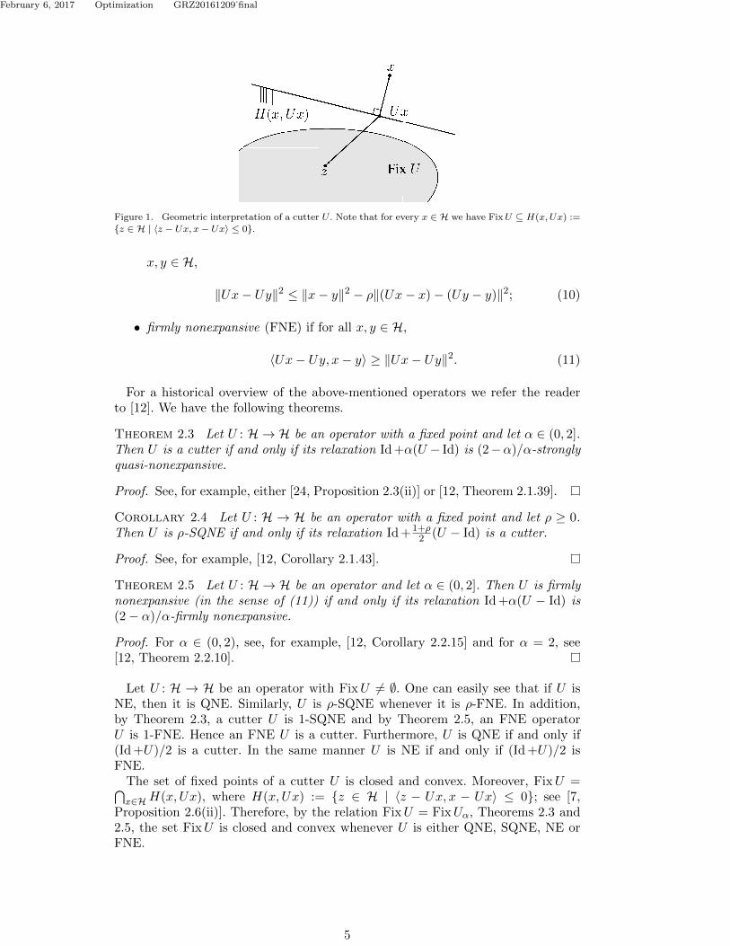
See Figure 1 for the geometric interpretation of a cutter.

Definition 2.2 Let U : H → H. We say that U is

• nonexpansive (NE) if for all x, y ∈ H,

‖Ux− Uy‖ ≤ ‖x− y‖; (9)

• ρ-firmly nonexpansive (ρ-FNE) [25, Definition 2.1], where ρ ≥ 0, if for all

4


Figure 1. Geometric interpretation of a cutter U . Note that for every x ∈ H we have FixU ⊆ H(x, Ux) :={z ∈ H | 〈z − Ux, x− Ux〉 ≤ 0}.

x, y ∈ H,

‖Ux− Uy‖2 ≤ ‖x− y‖2 − ρ‖(Ux− x)− (Uy − y)‖2; (10)

• firmly nonexpansive (FNE) if for all x, y ∈ H,

〈Ux− Uy, x− y〉 ≥ ‖Ux− Uy‖2. (11)

For a historical overview of the above-mentioned operators we refer the readerto [12]. We have the following theorems.

Theorem 2.3 Let U : H → H be an operator with a fixed point and let α ∈ (0, 2].Then U is a cutter if and only if its relaxation Id +α(U − Id) is (2−α)/α-stronglyquasi-nonexpansive.

Proof. See, for example, either [24, Proposition 2.3(ii)] or [12, Theorem 2.1.39].

Corollary 2.4 Let U : H → H be an operator with a fixed point and let ρ ≥ 0.Then U is ρ-SQNE if and only if its relaxation Id +1+ρ

2 (U − Id) is a cutter.

Proof. See, for example, [12, Corollary 2.1.43].

Theorem 2.5 Let U : H → H be an operator and let α ∈ (0, 2]. Then U is firmlynonexpansive (in the sense of (11)) if and only if its relaxation Id +α(U − Id) is(2− α)/α-firmly nonexpansive.

Proof. For α ∈ (0, 2), see, for example, [12, Corollary 2.2.15] and for α = 2, see[12, Theorem 2.2.10].

Let U : H → H be an operator with FixU 6= ∅. One can easily see that if U isNE, then it is QNE. Similarly, U is ρ-SQNE whenever it is ρ-FNE. In addition,by Theorem 2.3, a cutter U is 1-SQNE and by Theorem 2.5, an FNE operatorU is 1-FNE. Hence an FNE U is a cutter. Furthermore, U is QNE if and only if(Id +U)/2 is a cutter. In the same manner U is NE if and only if (Id +U)/2 isFNE.

The set of fixed points of a cutter U is closed and convex. Moreover, FixU =⋂x∈HH(x, Ux), where H(x, Ux) := {z ∈ H | 〈z − Ux, x − Ux〉 ≤ 0}; see [7,

Proposition 2.6(ii)]. Therefore, by the relation FixU = FixUα, Theorems 2.3 and2.5, the set FixU is closed and convex whenever U is either QNE, SQNE, NE orFNE.

5


Example 2.6 The metric projection onto a nonempty, closed and convex set C isFNE [12, Theorem 2.2.21]. Since FixPC = C 6= ∅, it is also a cutter. Therefore,for any α ∈ (0, 2], the relaxation Id +α(PC − Id) is ρ-FNE and ρ-SQNE, whereρ := (2− α)/α. Consequently, this relaxation is also NE and QNE.

Example 2.7 Let f : H → R be a convex continuous function with a nonemptysublevel set S(f, 0) := {x | f(x) ≤ 0}. Denote by ∂f(x) its subdifferential, thatis, ∂f(x) := {g ∈ H | f(y) − f(x) ≥ 〈g, y − x〉 for all y ∈ H}. By the continuityof f , the set ∂f(x) 6= ∅ for all x ∈ H (see [8, Proposition 16.3 and Proposition16.14]). For each x ∈ H, let gf (x) ∈ ∂f(x) be a given subgradient. The so-calledsubgradient projection relative to f is the operator Pf : H → H defined by

Pfx :=

{x− f(x)

‖gf (x)‖2 gf (x) if gf (x) 6= 0,

x otherwise.(12)

It is not difficult to see that FixPf = S(f, 0) (see [12, Lemma 4.2.5]) and thatPf is a cutter (see [12, Corollary 4.2.6]). Moreover, one may replace the condition“gf (x) 6= 0” in the definition of Pf by the condition “f(x) > 0”, which leads toan equivalent definition of the subgradient projection. Similarly, as in the previousexample, the relaxation Id +α(Pf − Id) is ρ-SQNE, where ρ := (2− α)/α.

The next theorem provides a relations between given SQNE operators U1, . . . , Umand their convex combinations or compositions.

Theorem 2.8 Let Ui : H → H be ρi-strongly quasi-nonexpansive, i ∈ I :={1, . . . ,m}, with

⋂i∈I FixUi 6= ∅ and let ρ := mini∈I ρi > 0. Then:

(i) the convex combination U :=∑

i∈I ωiUi, where ωi > 0, i ∈ I, and∑

i∈I ωi =1, is ρ-strongly quasi-nonexpansive;

(ii) the composition U := Um . . . U1 is ρm -strongly quasi-nonexpansive.

Moreover, in both cases,

FixU =⋂i∈I

FixUi. (13)

Proof. See, for example, [12, Theorems 2.1.48 and 2.1.50].

2.2. Regular operators

Definition 2.9 We say that a quasi-nonexpansive operator U : H → H is

(i) weakly regular (WR) if U − Id is demi-closed at 0, that is, if for any sequence{xk}∞k=0 ⊆ H and x ∈ H, we have

xk ⇀ xUxk − xk → 0

}=⇒ x ∈ FixU. (14)

(ii) boundedly regular (BR) if for any bounded sequence {xk}∞k=0 ⊆ H, we have

limk→∞

‖Uxk − xk‖ = 0 =⇒ limk→∞

d(xk,FixU) = 0. (15)

6


Weakly regular operators go back to papers by Browder and Petryshyn [11] andby Opial [36]. A prototypical version of condition (15) can be found in [37, Theorem1.2] by Petryshyn and Williamson. The term “boundedly regular” comes from [9]by Bauschke, Noll and Phan while the term “weakly regular” can be found in[33] by Kolobov, Reich and Zalas. Boundedly regular operators have been studiedunder the name approximately shrinking in [14, 16, 18, 19, 38, 47], whereas weaklyregular operators can be found, for example, in [15].

We have the following relation between weakly and boundedly regular operators:

Proposition 2.10 Let U : H → H be quasi-nonexpansive. Then the followingassertions hold:

(i) If U is boundedly regular, then U is weakly regular;(ii) If dimH <∞ and U is weakly regular, then U is boundedly regular.

Proof. See [19, Proposition 4.1].

It is worth mentioning that in a general Hilbert space the weak regularity of Uis only a necessary condition for implication (15) and even a firmly nonexpansivemapping may not have this property; see either [47, Example 2.9] or [29, Examples2.14 and 2.15]. It is also worth mentioning that Cegielski [14, Definition 4.4] hasrecently considered a demi-closednss condition referring to a family of operatorsinstead of a single one.

Example 2.11 Let C ⊆ H be closed and convex. Then the metric projection PCsatisfies the relation d(x,C) = ‖PCx− x‖ for every x ∈ H. Moreover, FixPC = C.Therefore PC is boundedly regular and, by Proposition 2.10, it is also weaklyregular.

Example 2.12 Let U : H → H be nonexpansive and assume that FixU 6= ∅. ThenU is weakly regular; see [36, Lemma 2]. Moreover, if H = Rn, then U is boundedlyregular.

Example 2.13 Let f : H → H and Pf be as in Example 2.7. If f is Lipschitzcontinuous on bounded sets, then Pf is weakly regular; see, for instance, [12, The-orem 4.2.7]. Note that by [6, Proposition 7.8], we can equivalently assume that fmaps bounded sets onto bounded sets or that the subdifferential of f is nonemptyand uniformly bounded on bounded sets. Moreover, if H = Rn, then Pf satisfiesall the above-mentioned conditions and consequently, by Proposition 2.10, Pf isboundedly regular.

2.3. Regularity of sets

Let Ci ⊆ H, i ∈ I, be closed and convex sets with a nonempty intersection C.Following Bauschke [4, Definition 2.1], we propose the following definition.

Definition 2.14 We say that the family C := {Ci | i ∈ I} is boundedly regular iffor any bounded sequence {xk}∞k=0 ⊆ H, the following implication holds:

limk→∞

maxi∈I

d(xk, Ci) = 0 =⇒ limk→∞

d(xk, C) = 0. (16)

Theorem 2.15 If at least one of the following conditions is satisfied:

(i) dimH <∞,

7


(ii) int⋂i∈I Ci 6= ∅,

(iii) each Ci is a half-space,

then the family C := {Ci | i ∈ I} is boundedly regular.

Proof. See [4, Fact 2.2].

For more properties of boundedly regular families of sets we refer the reader toBauschke’s PhD thesis [10] and to the review paper [6].

2.4. Hybrid steepest descent method

In this section we present a general convergence theorem for the hybrid steepestdescent method; compare with (5). In Section 3 we apply this theorem to a familyof relaxed metric projections Rk := Id +αk(PHk

− Id), which constitute our outer-approximation method. Before all this we recall the following technical lemma.

Lemma 2.16 Let {sk}∞k=0, {dk}∞k=0 ⊆ [0,∞) be given. The following conditions areequivalent:

(i) for any {nk}∞k=0 ⊆ {k}∞k=0, the following implication holds:

limk→∞

snk= 0 =⇒ lim

k→∞dnk

= 0; (17)

(ii) for any {nk}∞k=0 ⊆ {k}∞k=0 and for any ε > 0, there are k0 ≥ 0 and δ > 0such that for any k ≥ k0, the following implication holds:

snk< δ =⇒ dnk

< ε. (18)

Proof. See either [47, Lemma 3.15] or [29, Lemma 2.15].

Theorem 2.17 Let F : H → H be L-Lipschitz continuous and α-strongly mono-tone, and let C be closed and convex. Moreover, for each k = 0, 1, 2, . . ., letRk : H → H be ρk-SQNE such that C ⊆ FixRk and let λk ∈ [0,∞). Considerthe following hybrid steepest descent method:

z0 ∈ H; zk+1 := Rkzk − λkFRkzk. (19)

Then the sequence {zk}∞k=0 is bounded. Moreover, if ρ := infk ρk > 0,limk→∞ λk = 0 and there is an integer s ≥ 1 such that the implication

limk→∞

s−1∑l=0

‖Rnk−lznk−l − znk−l‖ = 0 =⇒ lim

k→∞d(znk , C) = 0 (20)

holds true for each subsequence {nk}∞k=0 ⊆ {k}∞k=0, then limk→∞ d(zk, C) = 0. If,in addition,

∑∞k=0 λk = ∞, then the sequence {zk}∞k=0 converges in norm to the

unique solution of VI(F , C).

The proof of this theorem can be found in [47, Theorem 3.16]. We include itbelow for the convenience of the reader.

Proof. Boundedness of {zk}∞k=0 follows from [18, Lemma 9].

8


To prove that d(zk, C) → 0 it suffices to show, by [18, Theorem 12], that forany ε > 0, there are k0 ≥ 0 and δ > 0 such that for any k ≥ k0, the followingimplication holds:

s−1∑l=0

ρk−l‖Rk−lzk−l − zk−l‖2 < δ =⇒ d2(zk, C) < ε. (21)

To this end, we define for each k = 0, 1, 2, . . . ,

sk :=

s−1∑l=0

ρk−l‖Rk−lzk−l − zk−l‖2 (22)

and

dk := d2(zk, C). (23)

It is easy to see that, by assumption, ρ > 0 and by (20), for any subsequence{nk}∞k=0 ⊆ {k}∞k=0, the following implication holds:

limk→∞

snk= 0 =⇒ lim

k→∞dnk

= 0. (24)

Clearly, Lemma 2.16 ((i)⇒(ii)) with nk ← k shows that implication (21) holds.Therefore, by [18, Theorem 12 (i)], we get limk→∞ d(zk, C) = 0.

To finish the proof, note that the assumption∑∞

k=0 λk = ∞, when combinedwith [18, Theorem 12 (v)], yields the assertion.

3. Outer approximation method

Theorem 3.1 Let F : H → H be L-Lipschitz continuous and α-strongly monotone,and let C ⊂ H be closed and convex. Moreover, for each k = 0, 1, 2, . . ., let Tk : H →H be a cutter such that C ⊆ FixTk and let λk ∈ [0,∞). Consider the followingouter approximation method:

x0 ∈ H; xk+1 := Rk(xk − λkFxk), for k = 0, 1, 2, . . . , (25)

where

Rk := Id +αk(PHk− Id), (26)

Hk := {z ∈ H | 〈z − Tkxk, xk − Tkxk〉 ≤ 0} (27)

and where αk ∈ [ε, 2− ε] is the user-chosen relaxation parameter for some ε > 0.Then the sequence {xk}∞k=0 is bounded. Moreover, if limk→∞ λk = 0 and there is

an integer s ≥ 1 such that the implication

limk→∞

s−1∑l=0

‖Tnk−lxnk−l − xnk−l‖ = 0 =⇒ lim

k→∞d(xnk , C) = 0 (28)

9


holds true for each subsequence {nk}∞k=0 ⊆ {k}∞k=0, then limk→∞ d(xk, C) = 0. If,in addition,

∑∞k=0 λk = ∞, then the sequence {xk}∞k=0 converges in norm to the


The detailed proof of this theorem is given in Subsection 3.1. For now we discussonly basic properties of this method with a geometric interpretation and a simplemotivation for the convergence conditions.

As we have already mentioned in the Introduction, Lipschitz continuity andstrong monotonicity of F guarantee the existence and uniqueness of a solution toVI(F , C).

Observe that for every k = 0, 1, 2, . . . , the set Hk is a half-space unless xk = Tkxk

in which case it is all of H. Therefore (25) has the following explicit form:

xk+1 = Rkzk =

{zk − αk 〈z

k−Tkxk, xk−Tkxk〉‖xk−Tkxk‖2 (xk − Tkxk) if zk /∈ Hk,

zk if zk ∈ Hk,(29)

where

zk := xk − λkFxk. (30)

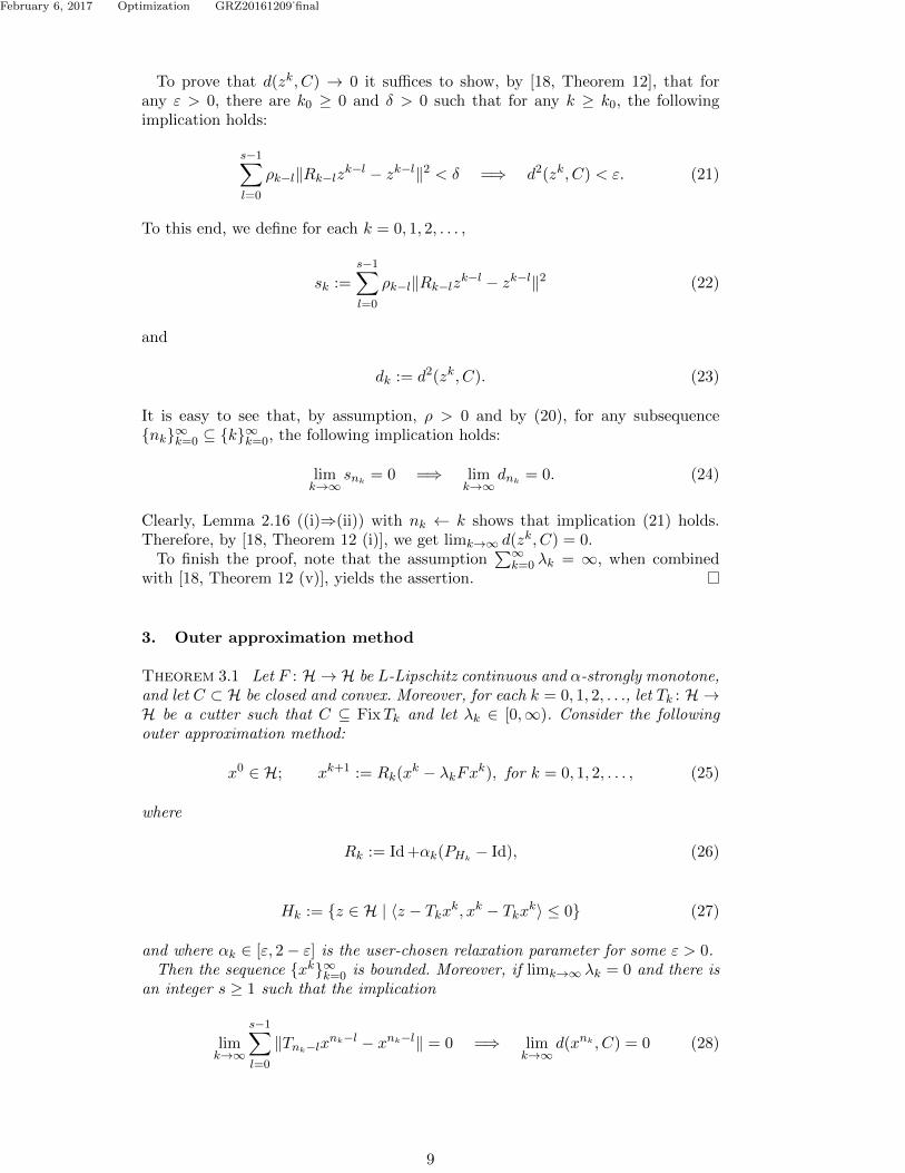
Moreover, since for every k = 0, 1, 2, . . ., the operator Tk is a cutter such thatC ⊆ FixTk, then the subset C is outerly approximated by Hk. Moreover, C ⊆FixTk ⊆ Hk. We illustrate the iterative method (25) in this case in Figure 2.

Figure 2. Illustration of the iterative step of the outer approximation method (25).

By imposing conditions on {λk}∞k=0, following Fukushima [28] and others, see [20],[17] and [29], we replace the fixed step size λ in the gradient projection method (2)by a null, non-summable sequence. This condition is quite common in optimizationtheory and, in particular, appears in the context of the HSD method (19); see,for example, the papers by Yamada and Ogura [46], Hirstoaga [32], Aoyama andKohsaka [2], Cegielski and Zalas [18, 19] and Cegielski and Al-Musallam [16]. Inmany cases, the choice of the sequence {λk}∞k=0 is more restrictive than the oneproposed in Theorem 3.1. Examples of such restrictions can be found in the papersby Halpern [31], Lions [35], Wittmann [42], Bauschke [5], Deutsch and Yamada[26], Yamada [45], Xu and Kim [44], Zeng et al. [49], Takahashi and Yamada [40],Aoyama and Kimura [1], and Zhang and He [50].

The condition (28) is essential as we now explain in detail. Although this con-dition imposes some regularity on the sequence {xk}∞k=0, the convergence of whichis under investigation, this does not reduce its generality. One could, for example,

10


assume a variant of (28), where instead of the trajectory of method (25), any arbi-trary sequence is used, as in [2, 41]. This, however, could be more difficult to verify,since an arbitrary sequence {xk}∞k=0 does not provide any additional informationconcerning its structure. By restricting our attention to trajectories generated bythe outer approximation method (25), we are able to utilize such a structure andtherefore the verification of (28) should require at most as much effort as its ver-ification for any arbitrary sequence. Notice, however, that (28) refers not only tothe sequence {xk}∞k=0, but first of all to the sequence of operators {Tk}∞k=0, whichdetermine method (25). We give now several simple examples where this condi-tion is satisfied. To make the introductory analysis simpler we assume that s = 1,Tk = T and C = FixT for some cutter T : H → H and for every k = 0, 1, 2, . . .. Itis not difficult to see that if T is boundedly regular and, in particular, if T = PC ,then (28) holds true. Now assume that H = Rn. If T is weakly regular and, inparticular, when T is either nonexpansive or T = Pf (see Examples 2.12 and 2.13),then again (28) is satisfied.

The parameter s > 1 in (28) enables us to use s-almost cyclic and s-intermittentcontrols. Examples for this case are presented in Section 4.

Historically, condition (28) in this form appeared in Zalas’ PhD thesis [47, Theo-rem 3.16] in the context of the HSD method, and more recently, in [29] in connectionwith the outer approximation method. Some of its weaker forms can be found in[18, Definition 19], [19, Definition 6.1] and [13, Definition 4.1]. Similar regularityconditions were proposed by many authors; see, for example, Bauschke et al. [6,Definition 3.7, Definition 4.8], Yamada et al. [46, Definition 1], Hirstoaga [32, Con-dition 2.2(iii)], Takahashi et al. [41, NST condition (I) ], Cegielski [12, Theorem3.6.2, Definition 5.8.5], and Aoyama et al. [2, Condition (Z)].

3.1. Convergence analysis

We begin this section with several simple observations. Let {xk}∞k=0 and {zk}∞k=0 betwo sequences generated by (25) and (30), respectively. Then for any k = 0, 1, 2, . . .,the vector zk+1 depends recursively on zk via the formula

z0 := x0 − λ0Fx0, zk+1 = Rkz

k − λk+1FRkzk. (31)

According to Example 2.6, for each k = 0, 1, 2, . . ., the operator Rk defined by(26) is ρk-SQNE with ρk := 2−αk

αk. Moreover, ρ := ε

2−ε satisfies the inequalities 0 <ρ ≤ infk ρk. Furthermore, for each k = 0, 1, 2, . . . , we get C ⊆ FixRk. Consequently,one may apply Theorem 2.17 to the sequences {zk}∞k=0 and {Rk}∞k=0, which is thekey idea in our convergence analysis. We begin with the following lemma:

Lemma 3.2 The following statements hold true:

(i) The sequences {xk}∞k=0 and {zk}∞k=0 are bounded;(ii) For any subsequence {nk}∞k=0 ⊆ {k}∞k=0, we have

limk→∞

(Rnkznk − znk) = 0 ⇐⇒ lim

k→∞(Tnk

xnk − xnk) = 0 (32)

⇐⇒ limk→∞

(xnk+1 − xnk) = 0 (33)

⇐⇒ limk→∞

(znk+1 − znk) = 0; (34)

(iii) If limk→∞ d(xnk , C) = 0, then all limits in (ii) are equal to zero;

11


(iv) limk→∞ d(xnk , C) = 0 if and only if limk→∞ d(znk , C) = 0;(v) limk→∞ x

nk = limk→∞ znk if at least one of the limits exists.

Proof. First we show that (i) holds true. Note that Theorem 2.17 (i), when com-bined with (31), leads to the boundedness of the sequence {zk}∞k=0. To show that{xk}∞k=0 is also bounded, fix z ∈ C. By the definition of xk+1 (see (25)), the quasi-nonexpansivity of Rk and the inclusion C ⊆ FixRk, it is easy to see that

‖xk+1 − z‖ = ‖Rkzk − z‖ ≤ ‖zk − z‖ (35)

for each k = 0, 1, 2, . . .. Therefore {xk}∞k=0 is also bounded, as asserted.Now we proceed to statement (ii). By (i), the sequence {xk}∞k=0 is bounded.

Therefore, by the Lipschitz continuity of F , there is M > 0 such that for eachk = 0, 1, 2 . . ., we have ‖Fxk‖ ≤M . Let {nk}∞k=0 ⊆ {k}∞k=0. Assume that ‖Tnk

xnk−xnk‖ 6= 0. Then, by (29), the Cauchy-Schwarz inequality, (30) and the triangleinequality,

‖Rnkznk − znk‖ = αnk

∥∥∥∥〈znk − Tnkxnk , xnk − Tnk

xnk〉‖xnk − Tnk

xnk‖2(xnk − Tnk

xnk)

∥∥∥∥≤ 2‖znk − Tnk

xnk‖ = 2 ‖xnk − λnkFxnk − Tnk

xnk‖

≤ 2 (‖Tnkxnk − xnk‖+ λnk

M) . (36)

Moreover, if ‖Tnkxnk − xnk‖ = 0, then Rnk

= Id and inequality (36) holds triviallyin this case.

Observe that for each k = 0, 1, 2, . . ., we have Tkxk = PHk

xk. Moreover, Rk =Id +αk(PHk

− Id) is NE, since PHkis FNE and αk ∈ [ε, 2 − ε] (see Example 2.6).

Hence, by the triangle inequality, (25) and (30), we have

‖Tnkxnk − xnk‖ =

1

αk

∥∥αk (PHnkxnk − xnk

)∥∥ ≤ 1

ε‖Rnk

xnk − xnk‖

≤ 1

ε

(‖Rnk

xnk − xnk+1‖+ ‖xnk+1 − xnk‖)

=1

ε

(‖Rnk

xnk −Rnkznk‖+ ‖xnk+1 − xnk‖

)≤ 1

ε

(λnk

M + ‖xnk+1 − xnk‖). (37)

Using (30) for xnk+1 and xnk together with the triangle inequality, we obtain

‖xnk+1 − xnk‖ ≤ ‖znk+1 − znk‖+M(λnk+1 + λnk). (38)

Moreover, by (31) applied to znk+1 and the triangle inequality,

‖znk+1 − znk‖ ≤ ‖Rnkznk − znk‖+ λnk+1M. (39)

The assumption that λk → 0, when combined with inequalities (36)–(39), yieldsthe equivalence (32).

Now we show that (iii) holds true. To this end, assume that

limk→∞

d(xnk , C) = 0. (40)

12


We claim that

limk→∞

‖xnk+1 − xnk‖ = 0. (41)

Indeed, by the triangle inequality, (25) and by the nonexpansivity of Rnk, we obtain

for all k ≥ 0,

‖xnk+1 − xnk‖ ≤ ‖xnk+1 −Rnkxnk‖+ ‖Rnk

xnk − xnk‖

= ‖Rnkznk −Rnk

xnk‖+ αnkd(xnk , Hnk

)

≤ ‖znk − xnk‖+ 2 d(xnk , Hnk)

≤ λnkM + 2 d(xnk , Hnk

), (42)

where the last equality follows from

λnkM ≥ ‖znk − xnk‖. (43)

Since for all k ≥ 0, C ⊆ Hnk, we have

d(xnk , Hnk) ≤ d(xnk , C). (44)

Thus

‖xnk+1 − xnk‖ ≤ λnkM + 2 d(xnk , C) (45)

and the right-hand side of the above inequality converges to zero by (40) and theassumption that λk → 0.

Statements (iv) and (v) follow directly from (43) and again by the assumptionthat λk → 0. This completes the proof.

Proof of Theorem 3.1. Let {zk}∞k=0 be the sequence defined in (30), correspondingto {xk}∞k=0. Moreover, let x∗ be the unique solution of VI(F , C). We show that{zk}∞k=0 converges in norm to x∗, which in view of Lemma 3.2 (v), yields the result.To this purpose, it suffices, by Theorem 2.17 and (31), to show that there is aninteger s ≥ 1 such that the implication

limk→∞

s−1∑l=0

‖Rnk−lznk−l − znk−l‖ = 0 =⇒ lim

k→∞d(znk , C) = 0 (46)

holds true for each subsequence {nk}∞k=0 ⊆ {k}∞k=0. Let {nk}∞k=0 ⊆ {k}∞k=0 andassume that the antecedent of (46) holds true, that is,

limk→∞

s−1∑l=0

‖Rnk−lznk−l − znk−l‖ = 0. (47)

Thus, using Lemma 3.2 (ii), we arrive at

limk→∞

s−1∑l=0

‖Tnk−lxnk−l − xnk−l‖ = 0. (48)

13


By (28), we get

limk→∞

d(xnk , C) = 0, (49)

which, when combined with Lemma 3.2 (iv), yields

limk→∞

d(znk , C) = 0. (50)

This completes the proof.

4. VIs over the common fixed point set

In this section we assume that C :=⋂i∈I Ci, where each Ci ⊆ H is closed and

convex and I := {1, . . . ,m}.

Theorem 4.1 Let F : H → H be L-Lipschitz continuous and α-strongly monotone,and assume that for each i ∈ I, we have Ci = FixUi for some cutter operatorUi : H → H. Let the sequence {xk}∞k=0 be defined by the outer approximation method(25)–(27) and for every k = 0, 1, 2, . . . , let Tk : H → H be defined either by asimultaneous

Tk :=∑i∈Ik

ωki Ui (51)

or a composition

Tk :=1

2(Id +

∏i∈Ik

Ui), (52)

algorithmic operator, where Ik ⊆ I,∑

i∈Ik ωki = 1 and 0 < ε ≤ ωki ≤ 1.

Then the sequence {xk}∞k=0 is bounded. Moreover, if limk→∞ λk = 0, Ui is bound-edly regular for every i ∈ I, {Ci | i ∈ I} is boundedly regular and there is an integers ≥ 1 such that I = Ik−s+1 ∪ . . . ∪ Ik for all k ≥ s, then limk→∞ d(xk, C) = 0. If,in addition,

∑∞k=0 λk = ∞, then the sequence {xk}∞k=0 converges in norm to the


Proof. We begin with several simple observations. The first one is that for eachk = 0, 1, 2, . . . , the operator Tk defined by either (51) or (52) is a cutter suchthat C ⊆ FixTk =

⋂i∈Ik FixUi. This follows from Theorem 2.8 and Corollary

2.4. Therefore it is reasonable to consider an outer approximation method withthese particular algorithmic operators Tk. Consequently, by Theorem 3.1, {xk}∞k=0is bounded.

Another observation is that, by [38, Lemma 3.5], for each subsequence {nk}∞k=0 ⊆{k}∞k=0 and l ∈ {0, . . . , s− 1}, we have

limk→∞


k→∞maxi∈Ink−l

d(xnk−l,FixUi) = 0. (53)

In order to complete the proof, in view of Theorem 3.1 and the bounded regularity

14


of {Ci | i ∈ I}, it suffices to show that

limk→∞

s−1∑l=0


k→∞maxi∈I

d(xnk ,FixUi) = 0. (54)

Indeed, assume that the left-hand side of (54) holds, that is,

limk→∞

s−1∑l=0

‖Tnk−lxnk−l − xnk−l‖ = 0, (55)

which, by (53), implies that for each l = 0, 1, . . . , s− 1,

limk→∞

maxj∈Ink−l

d(xnk−l,FixUj) = 0. (56)

Again by (55), the triangle inequality and Lemma 3.2 (ii) applied to nk ← (nk− l),for every l = 1, 2, . . . , s− 1, we get

limk→∞

‖xnk − xnk−l‖ = 0. (57)

Let i ∈ I. The control {Ik}∞k=0 satisfies I = Ink∪ Ink−1∪ . . . Ink−s+1 for all k ≥ 0.

Consequently, for each k ≥ s− 1, there is lk ∈ {0, . . . , s− 1} such that i ∈ Ink−lk .By the definition of the metric projection and the triangle inequality, we have

d(xnk ,FixUi) = ‖PFixUixnk − xnk‖ ≤ ‖PFixUi

xnk−lk − xnk‖

≤ ‖PFixUixnk−lk − xnk−lk‖+ ‖xnk − xnk−lk‖

= d(xnk−lk ,FixUi) + ‖xnk − xnk−lk‖. (58)

Therefore (58), (57) and (56) imply that

limk→∞

maxi∈I

d(xnk ,FixUi) = 0, (59)

which completes the proof.

Theorem 4.2 Let F : H → H be L-Lipschitz continuous and α-strongly monotone,and assume that for each i ∈ I, we have Ci = FixUi = p−1

i (0) for some cutteroperator Ui : H → H and a proximity function pi : H → [0,∞). Let the sequence{xk}∞k=0 be defined by the outer approximation method (25)–(27) and for everyk = 0, 1, 2, . . . , let Tk : H → H be defined by the maximum proximity algorithmicoperator

Tk := Uik , where ik = argmaxi∈Ik

pi(xk), (60)

and where Ik ⊆ I.Then the sequence {xk}∞k=0 is bounded. Moreover, if limk→∞ λk = 0, Ui is

boundedly regular for every i ∈ I, {Ci | i ∈ I} is boundedly regular, there isan integer s ≥ 1 such that I = Ik−s+1 ∪ . . . ∪ Ik for all k ≥ s and for everybounded {yk}∞k=0 ⊆ H, we have limk→∞ pi(y

k) = 0⇐⇒ limk→∞ d(yk, Ci) = 0, then

15


limk→∞ d(xk, C) = 0. If, in addition,∑∞

k=0 λk = ∞, then the sequence {xk}∞k=0converges in norm to the unique solution of VI(F , C).

Proof. Note that one can easily see that (53) holds true for Tk defined in (60).Therefore the proof remains the same as for Theorem 4.1.

This type of the maximum proximity algorithmic operator can be found in [33]although its projected variant can also be found in [12, Section 5.8.4.1].

The relation Ci = FixUi = p−1i (0) becomes clearer once we assume that the

computation of pi is at most as difficult as the evaluation of Ui and this is at mostas difficult as projecting onto Ci. These assumptions are satisfied if, for example,the set Ci = {z ∈ H | fi(z) ≤ 0} is a sublevel set of a convex functional fi, theoperator Ui = Pfi is a subgradient projection and the proximity pi = f+

i , wheref+i (x) := max{0, fi(x)}. The remaining part is to verify whether pi(y

k) → 0 ⇐⇒d(yk, Ci)→ 0, which we show in the following lemma.

Lemma 4.3 Let fi : Rn → R be convex and assume that S(fi, 0) 6= ∅, i ∈ I.Moreover, let {ik}∞k=0 ⊆ I. Then for every bounded sequence {yk}∞k=0, we have

limk→∞

‖Pfikyk−yk‖ = 0 ⇐⇒ lim

k→∞f+ik

(yk) = 0 ⇐⇒ limk→∞

d(yk, S(fik , 0)) = 0.

(61)

Proof. First, assume that I = {i}. Observe that the implications “=⇒” followdirectly from the proof of [18, Lemma 24], which indicates that Pfi is boundedlyregular. Note that since Pfi is a cutter, we have ‖Pfix − x‖ ≤ d(x,FixPfi) forevery x ∈ Rn, where FixPfi = S(fi, 0). This shows equivalence for I = {i}. Nowwe assume that I = {1, . . . ,m}. To complete the proof we decompose the setK = {0, 1, 2, . . .} into subsets Ki := {k ∈ K | ik = i}. After doing this, we canrepeat the first argument for every component Ki, separately.

The condition that I ⊆ Ik−s+1 ∪ . . . ∪ Ik for all k ≥ s and some s ≥ 1 appearsin the literature as s-intermittent control, whereas for |Ik| = 1 it is known as s-almost cyclic; see, for example [6, Definition 3.18]. We comment now on a practicalrealization of this condition in the context of projection and subgradient projectionalgorithms.

Example 4.4 (Block projection algorithms) Let C =⋂i∈I Ci, and set Ui = PCi

and pi = d(·, Ci). For a fixed block size 1 ≤ b ≤ m, let I0 = {1, . . . , b} and let lk bethe last index from a given Ik. We define Ik+1 = ({lk, . . . , lk + b− 1} mod b) + 1.In principle, Ik consists of the next b indices following lk, which in the case of bdividing m is nothing but a cyclic way of changing fixed blocks I1, . . . , Im/b, eachof them of size b. We can visualize the definition of Ik in the following way:

1, 2, . . . , b︸︷︷︸I0

, b+ 1, b+ 2, . . . , 2b︸︷︷︸I1

, . . . ,m− 1,m, 1, 2, . . . , b− 2︸︷︷︸Ik

, b− 1, b, . . .︸︷︷︸Ik+1

(62)

Following Theorems 4.1 and 4.2, we have the following examples of projectionalgorithmic operators which determine our outer approximation method:

a) cyclic projection operator: Tk = PC[k], where [k] = (k mod m) + 1;

b) remotest-set projection operator: Tk := PCik, where ik = argmaxi∈Ik d(xk, Ci);

see Theorem 4.2;c) simultaneous projection operator: Tk := 1

|Ik|∑

i∈Ik PCi;

16


d) composition projection operator: Tk := 12(Id +

∏i∈Ik PCi

).

Example 4.5 (Block subgradient projection algorithms in Rn) Let C =⋂i∈I Ci,

where Ci = {z ∈ Rn | fi(z) ≤ 0} and fi : Rn → R is convex. We set Ui = Pfi ,see Example 2.7, and pi = f+

i . For a fixed block size 1 ≤ b ≤ m we define Ik asin Example 4.4. Again, following Theorems 4.1 and 4.2, we have the following ex-amples of subgradient projection algorithmic operators which determine our outerapproximation method:

a) cyclic subgradient projection operator: Tk = Pf[k], where [k] = (k mod m) + 1;

b) most-violated constraint subgradient projection operator: Tk := Pfik , where

ik = argmaxi∈Ik f+i (xk); see Theorem 4.2 and Lemma 4.3;

c) simultaneous subgradient projection operator: Tk := 1|Ik|∑

i∈Ik Pfi ;

d) composition subgradient projection operator: Tk := 12(Id +

∏i∈Ik Pfi).

Example 4.6 (Augmented block size) Using algorithmic operators over a block ofsize smaller than m is of practical importance when m is a large number. Thereforewe propose to slightly modify the definition of Ik from Examples 4.4 and 4.5 toobtain an augmented block, where |Ik| = bk ≥ b. Indeed, we define Ik in a simi-lar “cyclic” order, but for the simultaneous and maximum proximity algorithmicoperators we want Ik to satisfy

|{i ∈ Ik | constraint i is active at xk}| = b (63)

if the number of active constraints is greater than or equal b. If this is not possible,then we simply set Ik := I. The case of composition methods is slightly different,where we demand that

|{it ∈ Ik = (i1, . . . , ibk) | constraint it is active at Uit−1. . . U1x

k}| = b (64)

and we set Ik := I if condition (64) cannot be satisfied. Therefore, for a fixed b, wedenote the size of the augmented block by |Ik| = b+. Using algorithmic operatorsover the augmented block, we may significantly accelerate the outer approximationmethod as we show in the last section of this paper.

Remark 4.7 We would like to mention that there are many more algorithmicoperators Tk available in the literature that one could combine with the outerapproximation method; see, for example, the definition of dynamic string averagingprojection from [22], modular string averaging from [38] and double-layer fixedpoint algorithm from [33]. Moreover, there are many more adaptive definitions ofthe convex combinations coefficients, for example,

ωki :=pi(x

k)∑i∈Ik pi(x

k)or ωki :=

‖Uixk − xk‖∑i∈Ik ‖Uixk − xk‖

. (65)

Nevertheless, in order to ease the readability of this paper, we focus only on themaximum proximity, simultaneous and composition variants of the outer approxi-mation method.

Remark 4.8 (Polyhedral case and cyclic control) Consider the outer approximationmethod (25) combined with a cyclic control with relaxation parameters αk equalto 1, that is, Tk = U[k] and [k] = (k mod m) + 1. If for each i ∈ I the operatorUi is a metric projection onto a half-space Ci = {z ∈ H | 〈ai, z〉 ≤ βi}, then for

17


each k = 0, 1, 2, . . . , we have Hk = C[k] whenever xk /∈ C[k] and Hk = H otherwise.Therefore in this case we can rewrite method (25) in the following form:

x0 ∈ H; xk+1 := PC[k]

(xk − λkFxk

), for k = 0, 1, 2, . . . . (66)

5. Numerical results

We consider the following best approximation problem:

Find x∗ ∈ Argminz∈C

1

2‖z − a‖2, (67)

where a ∈ R20 is a given vector and C := {z ∈ R20 | Az ≤ b} for some matrixA ∈ R100×20. Thus, for each i ∈ I := {1, . . . , 100}, the subset Ci = {z ∈ R20 |〈ai, z〉 ≤ bi} is a half-space. It is not difficult to see that this problem is equivalentto the variational inequality with F := Id−a and C =

⋂i∈I Ci. We set

pi(x) := (〈ai, x〉 − bi)+; Uix := PCix = x− pi(x)

‖ai‖2ai (68)

and λk := 1k+1 for k = 0, 1, 2, . . .. We recall that (x)+ := max{0, x}.

Following Theorems 4.1 and 4.2, we consider the outer approximation method(25)–(27) with the following projection operators (PO):

• Cyclic PO: Tk := U[k], where [k] := (k mod 100) + 1;

• Maximum proximity PO: Tk := Uik , where ik := argmaxi∈Ik pi(xk);

• Simultaneous PO: Tk := 1|Ik|∑

i∈Ik PCi;

• Composition PO: Tk := 12(Id +

∏i∈Ik PCi

)

For block algorithms we apply two types of control {Ik}∞k=0. The first one with afixed block size |Ik| = b and the second one, with augmented block size |Ik| = b+;see Examples 4.4 and 4.6, respectively.

For every algorithm we perform 100 simulations, while sharing the same set ofrandomly generated test problems. We run every algorithm till it reaches 5000iterations. After running all of the simulations, for every iterate we compute theerror ‖xk − x∗‖, where x∗ is the given solution provided by MATLAB fmincon

solver. In order to compare our algorithms, we consider the quantity

log10

(‖xk − x∗‖‖x0 − x∗‖

). (69)

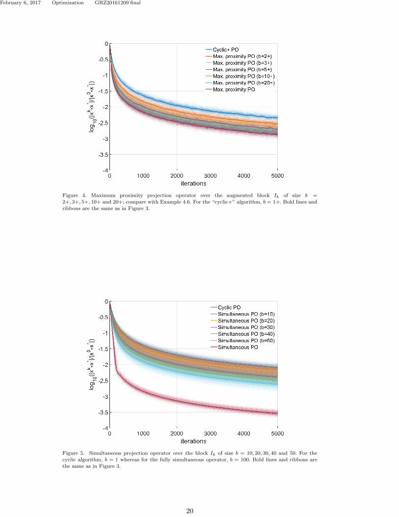
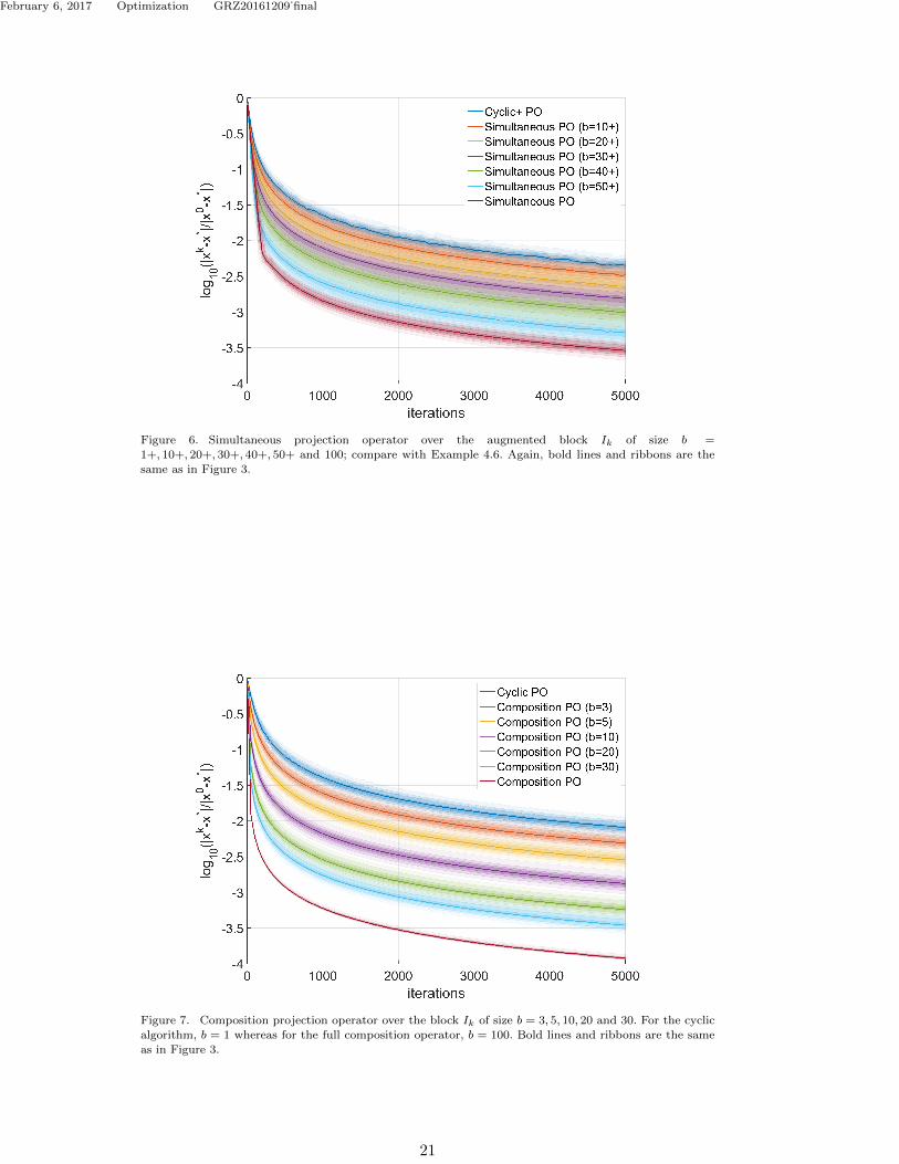
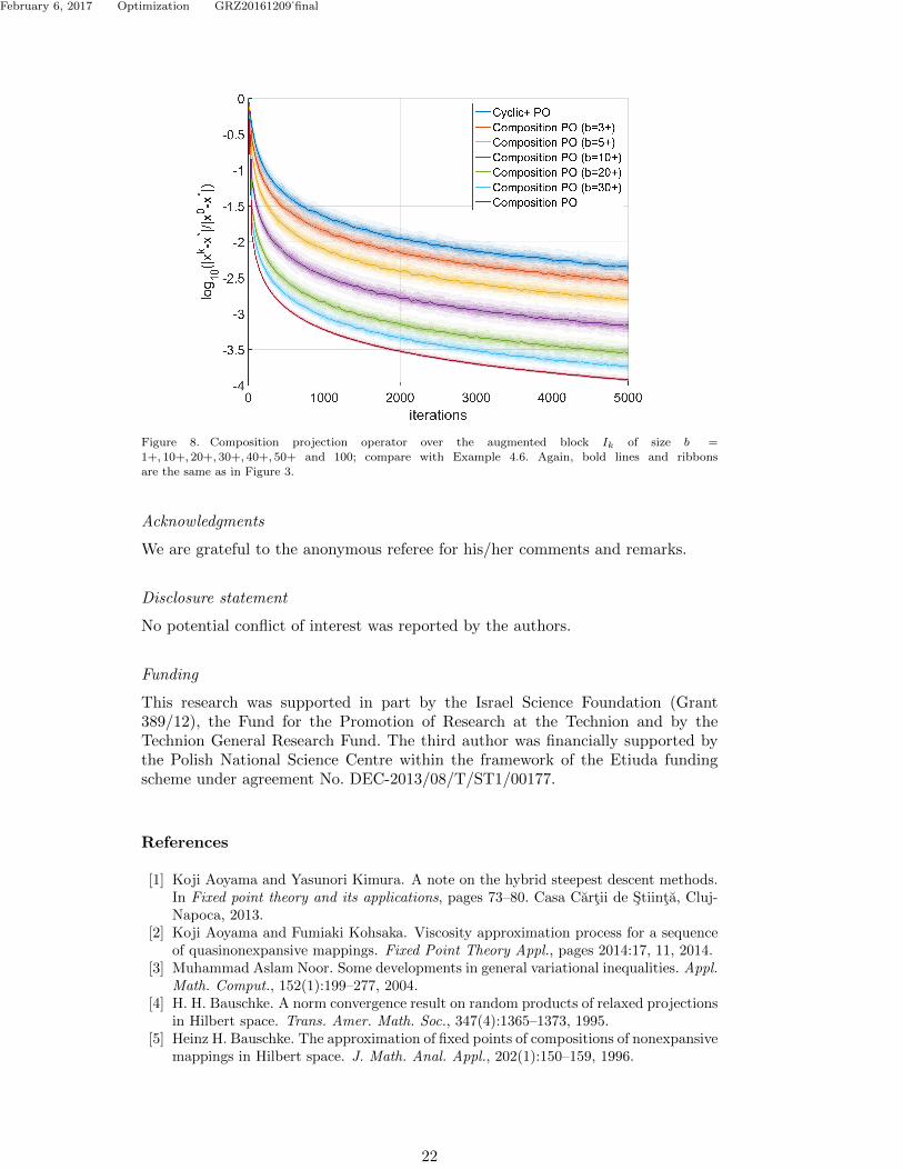
The bold line in Figures 3-8 indicates the median computed for (69). The ribbonplot represents concentrations of order 20, 40, 60 and 80% around the median. Weplot all the information per every 50 iterative steps.

We present now several observations that we have made after running the nu-merical simulations.

a) The outer approximation method equipped with the composition algorithmicoperator outperforms every other method we have considered;

b) The convergence speed for the maximum proximity, simultaneous and compo-sition methods is monotone with respect to a block size, that is, the larger the

18


block is, the faster the convergence we can expect. Therefore for b = 100 weexpect the best convergence profile for all of the methods;

c) The augmented block strategy described in Example 4.6 accelerates the conver-gence speed. This acceleration is significant in the simultaneous and compositioncases;

d) There is no need to use large blocks with b = m. For the maximum proximityit suffices to take b = 20 and for augmented version even b = 10+. Similarly,for composition type methods b = 30 and b = 20+ are quite close to the caseof b = 100. This can also be seen for the simultaneous projection operator withb = 50+.

Figure 3. Maximum proximity projection operator over the block Ik of size b = 2, 3, 5, 10 and 20. For the

cyclic algorithm, b = 1. A bold line indicates the median computed for (69). The ribbon plot representsconcentrations of order 20, 40, 60 and 80% around the median.

19


Figure 4. Maximum proximity projection operator over the augmented block Ik of size b =

2+, 3+, 5+, 10+ and 20+; compare with Example 4.6. For the “cyclic+” algorithm, b = 1+. Bold lines and

ribbons are the same as in Figure 3.

Figure 5. Simultaneous projection operator over the block Ik of size b = 10, 20, 30, 40 and 50. For thecyclic algorithm, b = 1 whereas for the fully simultaneous operator, b = 100. Bold lines and ribbons are

the same as in Figure 3.

20


Figure 6. Simultaneous projection operator over the augmented block Ik of size b =

1+, 10+, 20+, 30+, 40+, 50+ and 100; compare with Example 4.6. Again, bold lines and ribbons are the

same as in Figure 3.

Figure 7. Composition projection operator over the block Ik of size b = 3, 5, 10, 20 and 30. For the cyclicalgorithm, b = 1 whereas for the full composition operator, b = 100. Bold lines and ribbons are the same

as in Figure 3.

21


Figure 8. Composition projection operator over the augmented block Ik of size b =

1+, 10+, 20+, 30+, 40+, 50+ and 100; compare with Example 4.6. Again, bold lines and ribbons

are the same as in Figure 3.

Acknowledgments

We are grateful to the anonymous referee for his/her comments and remarks.

Disclosure statement

No potential conflict of interest was reported by the authors.

Funding

This research was supported in part by the Israel Science Foundation (Grant389/12), the Fund for the Promotion of Research at the Technion and by theTechnion General Research Fund. The third author was financially supported bythe Polish National Science Centre within the framework of the Etiuda fundingscheme under agreement No. DEC-2013/08/T/ST1/00177.

References

[1] Koji Aoyama and Yasunori Kimura. A note on the hybrid steepest descent methods.In Fixed point theory and its applications, pages 73–80. Casa Cartii de Stiinta, Cluj-Napoca, 2013.

[2] Koji Aoyama and Fumiaki Kohsaka. Viscosity approximation process for a sequenceof quasinonexpansive mappings. Fixed Point Theory Appl., pages 2014:17, 11, 2014.

[3] Muhammad Aslam Noor. Some developments in general variational inequalities. Appl.Math. Comput., 152(1):199–277, 2004.

[4] H. H. Bauschke. A norm convergence result on random products of relaxed projectionsin Hilbert space. Trans. Amer. Math. Soc., 347(4):1365–1373, 1995.

[5] Heinz H. Bauschke. The approximation of fixed points of compositions of nonexpansivemappings in Hilbert space. J. Math. Anal. Appl., 202(1):150–159, 1996.

22


[6] Heinz H. Bauschke and Jonathan M. Borwein. On projection algorithms for solvingconvex feasibility problems. SIAM Rev., 38(3):367–426, 1996.

[7] Heinz H. Bauschke and Patrick L. Combettes. A weak-to-strong convergence principlefor Fejer-monotone methods in Hilbert spaces. Math. Oper. Res., 26(2):248–264, 2001.

[8] Heinz H. Bauschke and Patrick L. Combettes. Convex analysis and monotone operatortheory in Hilbert spaces. CMS Books in Mathematics/Ouvrages de Mathematiques dela SMC. Springer, New York, 2011. With a foreword by Hedy Attouch.

[9] Heinz H. Bauschke, Dominikus Noll, and Hung M. Phan. Linear and strong conver-gence of algorithms involving averaged nonexpansive operators. J. Math. Anal. Appl.,421(1):1–20, 2015.

[10] Heinz Hermann Bauschke. Projection algorithms and monotone operators. PhD thesis,Simon Fraser University, Canada, 1996.

[11] F. E. Browder and W. V. Petryshyn. The solution by iteration of nonlinear functionalequations in Banach spaces. Bull. Amer. Math. Soc., 72:571–575, 1966.

[12] Andrzej Cegielski. Iterative methods for fixed point problems in Hilbert spaces, volume2057 of Lecture Notes in Mathematics. Springer, Heidelberg, 2012.

[13] Andrzej Cegielski. Extrapolated simultaneous subgradient projection method for vari-ational inequality over the intersection of convex subsets. J. Nonlinear Convex Anal.,15(2):211–218, 2014.

[14] Andrzej Cegielski. Application of quasi-nonexpansive operators to an iterative methodfor variational inequality. SIAM J. Optim., 25(4):2165–2181, 2015.

[15] Andrzej Cegielski. General method for solving the split common fixed point problem.J. Optim. Theory Appl., 165(2):385–404, 2015.

[16] Andrzej Cegielski and Fadhel Al-Musallam. Strong convergence of a hybrid steepestdescent method for the split common fixed point problem. Optimization, 65(7):1463–1476, 2016.

[17] Andrzej Cegielski, Aviv Gibali, Simeon Reich, and Rafa l Zalas. An algorithm for solv-ing the variational inequality problem over the fixed point set of a quasi-nonexpansiveoperator in Euclidean space. Numer. Funct. Anal. Optim., 34(10):1067–1096, 2013.

[18] Andrzej Cegielski and Rafa l Zalas. Methods for variational inequality problem overthe intersection of fixed point sets of quasi-nonexpansive operators. Numer. Funct.Anal. Optim., 34(3):255–283, 2013.

[19] Andrzej Cegielski and Rafa l Zalas. Properties of a class of approximately shrinkingoperators and their applications. Fixed Point Theory, 15(2):399–426, 2014.

[20] Yair Censor and Aviv Gibali. Projections onto super-half-spaces for monotone vari-ational inequality problems in finite-dimensional space. J. Nonlinear Convex Anal.,9(3):461–475, 2008.

[21] Yair Censor and Alexander Segal. The split common fixed point problem for directedoperators. J. Convex Anal., 16(2):587–600, 2009.

[22] Yair Censor and Alexander J. Zaslavski. Convergence and perturbation resilience ofdynamic string-averaging projection methods. Comput. Optim. Appl., 54(1):65–76,2013.

[23] Renu Chugh and Rekha Rani. Variational inequalities and fixed point problems: asurvey. International Journal of Applied Mathematical Research, 3(3):301–326, 2014.

[24] Patrick L. Combettes. Quasi-Fejerian analysis of some optimization algorithms. InInherently parallel algorithms in feasibility and optimization and their applications(Haifa, 2000), volume 8 of Stud. Comput. Math., pages 115–152. North-Holland, Am-sterdam, 2001.

[25] G. Crombez. A hierarchical presentation of operators with fixed points on Hilbertspaces. Numer. Funct. Anal. Optim., 27(3-4):259–277, 2006.

[26] Frank Deutsch and Isao Yamada. Minimizing certain convex functions over the in-tersection of the fixed point sets of nonexpansive mappings. Numer. Funct. Anal.Optim., 19(1-2):33–56, 1998.

[27] Francisco Facchinei and Jong-Shi Pang. Finite-dimensional variational inequalitiesand complementarity problems. Vol. I and II. Springer Series in Operations Research.Springer-Verlag, New York, 2003.

23


[28] Masao Fukushima. A relaxed projection method for variational inequalities. Math.Programming, 35(1):58–70, 1986.

[29] Aviv Gibali, Simeon Reich, and Rafa l Zalas. Iterative methods for solving variationalinequalities in Euclidean space. J. Fixed Point Theory Appl., 17(4):775–811, 2015.

[30] A. A. Goldstein. Convex programming in Hilbert space. Bull. Amer. Math. Soc.,70:709–710, 1964.

[31] Benjamin Halpern. Fixed points of nonexpanding maps. Bull. Amer. Math. Soc.,73:957–961, 1967.

[32] Sever A. Hirstoaga. Iterative selection methods for common fixed point problems. J.Math. Anal. Appl., 324(2):1020–1035, 2006.

[33] Victor I. Kolobov, Simeon Reich, and Rafa Zalas. Weak, strong and linear convergenceof a double-layer fixed point algorithm. Preprint, 2016.

[34] E.S. Levitin and B.T. Polyak. Constrained minimization methods. USSR Computa-tional Mathematics and Mathematical Physics, 6(5):1–50, 1966.

[35] Pierre-Louis Lions. Approximation de points fixes de contractions. C. R. Acad. Sci.Paris Ser. A-B, 284(21):A1357–A1359, 1977.

[36] Zdzis law Opial. Weak convergence of the sequence of successive approximations fornonexpansive mappings. Bull. Amer. Math. Soc., 73:591–597, 1967.

[37] W. V. Petryshyn and T. E. Williamson, Jr. Strong and weak convergence of thesequence of successive approximations for quasi-nonexpansive mappings. J. Math.Anal. Appl., 43:459–497, 1973.

[38] Simeon Reich and Rafa l Zalas. A modular string averaging procedure for solvingthe common fixed point problem for quasi-nonexpansive mappings in Hilbert space.Numer. Algorithms, 72(2):297–323, 2016.

[39] Konstantinos Slavakis, Isao Yamada, and Kohichi Sakaniwa. Computation of symmet-ric positive definite toeplitz matrices by the hybrid steepest descent method. SignalProcessing, 83(5):1135–1140, 5 2003.

[40] Noriyuki Takahashi and Isao Yamada. Parallel algorithms for variational inequalitiesover the Cartesian product of the intersections of the fixed point sets of nonexpansivemappings. J. Approx. Theory, 153(2):139–160, 2008.

[41] Wataru Takahashi, Yukio Takeuchi, and Rieko Kubota. Strong convergence theoremsby hybrid methods for families of nonexpansive mappings in Hilbert spaces. J. Math.Anal. Appl., 341(1):276–286, 2008.

[42] Rainer Wittmann. Approximation of fixed points of nonexpansive mappings. Arch.Math. (Basel), 58(5):486–491, 1992.

[43] Naihua Xiu and Jianzhong Zhang. Some recent advances in projection-type methodsfor variational inequalities. In Proceedings of the International Conference on RecentAdvances in Computational Mathematics (ICRACM 2001) (Matsuyama), volume 152,pages 559–585, 2003.

[44] H. K. Xu and T. H. Kim. Convergence of hybrid steepest-descent methods for varia-tional inequalities. J. Optim. Theory Appl., 119(1):185–201, 2003.

[45] Isao Yamada. The hybrid steepest descent method for the variational inequality prob-lem over the intersection of fixed point sets of nonexpansive mappings. In Inherentlyparallel algorithms in feasibility and optimization and their applications (Haifa, 2000),volume 8 of Stud. Comput. Math., pages 473–504. North-Holland, Amsterdam, 2001.

[46] Isao Yamada and Nobuhiko Ogura. Hybrid steepest descent method for variationalinequality problem over the fixed point set of certain quasi-nonexpansive mappings.Numer. Funct. Anal. Optim., 25(7-8):619–655, 2004.

[47] Rafa lZalas. Variational Inequalities for Fixed Point Problems of Quasi-nonexpansiveOperators. PhD thesis, University of Zielona Gora, Zielona Gora, Poland, 2014. InPolish.

[48] Eberhard Zeidler. Nonlinear functional analysis and its applications. III. Springer-Verlag, New York, 1985. Variational methods and optimization, Translated from theGerman by Leo F. Boron.

[49] L. C. Zeng, N. C. Wong, and J. C. Yao. Convergence analysis of modified hybridsteepest-descent methods with variable parameters for variational inequalities. J.

24


Optim. Theory Appl., 132(1):51–69, 2007.[50] Cuijie Zhang and Songnian He. A general iterative algorithm for an infinite family of

nonexpansive operators in Hilbert spaces. Fixed Point Theory Appl., pages 2013:138,15, 2013.

25

Outer Approximation Methods for Solving Variational ... · Outer Approximation Methods for Solving...

Documents

Transcript of Outer Approximation Methods for Solving Variational ... · Outer Approximation Methods for Solving...