Solving ODE in MATLAB

P. Howard

Fall 2007

Contents

1 Finding Explicit Solutions 1

1.1 First Order Equations . . . . . . . . . . . . . . . . . . . . . . . . . . . . . . 21.2 Second and Higher Order Equations . . . . . . . . . . . . . . . . . . . . . . . 31.3 Systems . . . . . . . . . . . . . . . . . . . . . . . . . . . . . . . . . . . . . . 3

2 Finding Numerical Solutions 4

2.1 First-Order Equations with Inline Functions . . . . . . . . . . . . . . . . . . 52.2 First Order Equations with M-files . . . . . . . . . . . . . . . . . . . . . . . 72.3 Systems of ODE . . . . . . . . . . . . . . . . . . . . . . . . . . . . . . . . . . 72.4 Passing Parameters . . . . . . . . . . . . . . . . . . . . . . . . . . . . . . . . 102.5 Second Order Equations . . . . . . . . . . . . . . . . . . . . . . . . . . . . . 10

3 Laplace Transforms 10

4 Boundary Value Problems 11

5 Event Location 12

6 Numerical Methods 15

6.1 Euler’s Method . . . . . . . . . . . . . . . . . . . . . . . . . . . . . . . . . . 156.2 Higher order Taylor Methods . . . . . . . . . . . . . . . . . . . . . . . . . . 18

7 Advanced ODE Solvers 20

7.1 Stiff ODE . . . . . . . . . . . . . . . . . . . . . . . . . . . . . . . . . . . . . 21

1 Finding Explicit Solutions

MATLAB has an extensive library of functions for solving ordinary differential equations.In these notes, we will only consider the most rudimentary.

1

1.1 First Order Equations

Though MATLAB is primarily a numerics package, it can certainly solve straightforwarddifferential equations symbolically.1 Suppose, for example, that we want to solve the firstorder differential equation

y′(x) = xy. (1.1)

We can use MATLAB’s built-in dsolve(). The input and output for solving this problem inMATLAB is given below.

>>y = dsolve(’Dy = y*x’,’x’)y = C1*exp(1/2*xˆ2)

Notice in particular that MATLAB uses capital D to indicate the derivative and requires thatthe entire equation appear in single quotes. MATLAB takes t to be the independent variableby default, so here x must be explicitly specified as the independent variable. Alternatively,if you are going to use the same equation a number of times, you might choose to define itas a variable, say, eqn1.

>>eqn1 = ’Dy = y*x’eqn1 =Dy = y*x>>y = dsolve(eqn1,’x’)y = C1*exp(1/2*xˆ2)

To solve an initial value problem, say, equation (1.1) with y(1) = 1, use

>>y = dsolve(eqn1,’y(1)=1’,’x’)y =1/exp(1/2)*exp(1/2*xˆ2)

or

>>inits = ’y(1)=1’;>>y = dsolve(eqn1,inits,’x’)y =1/exp(1/2)*exp(1/2*xˆ2)

Now that we’ve solved the ODE, suppose we want to plot the solution to get a rough idea ofits behavior. We run immediately into two minor difficulties: (1) our expression for y(x) isn’tsuited for array operations (.*, ./, .ˆ), and (2) y, as MATLAB returns it, is actually a symbol(a symbolic object). The first of these obstacles is straightforward to fix, using vectorize().For the second, we employ the useful command eval(), which evaluates or executes textstrings that constitute valid MATLAB commands. Hence, we can use

1Actually, whenever you do symbolic manipulations in MATLAB what you’re really doing is calling

Maple.

2

>>x = linspace(0,1,20);>>z = eval(vectorize(y));>>plot(x,z)

You may notice a subtle point here, that eval() evaluates strings (character arrays), and y,as we have defined it, is a symbolic object. However, vectorize converts symbolic objectsinto strings.

1.2 Second and Higher Order Equations

Suppose we want to solve and plot the solution to the second order equation

y′′(x) + 8y′(x) + 2y(x) = cos(x); y(0) = 0, y′(0) = 1. (1.2)

The following (more or less self-explanatory) MATLAB code suffices:

>>eqn2 = ’D2y + 8*Dy + 2*y = cos(x)’;>>inits2 = ’y(0)=0, Dy(0)=1’;>>y=dsolve(eqn2,inits2,’x’)y =1/65*cos(x)+8/65*sin(x)+(-1/130+53/1820*14ˆ(1/2))*exp((-4+14ˆ(1/2))*x)-1/1820*(53+14ˆ(1/2))*14ˆ(1/2)*exp(-(4+14ˆ(1/2))*x)>>z = eval(vectorize(y));>>plot(x,z)

1.3 Systems

Suppose we want to solve and plot solutions to the system of three ordinary differentialequations

x′(t) = x(t) + 2y(t) − z(t)

y′(t) = x(t) + z(t)

z′(t) = 4x(t) − 4y(t) + 5z(t). (1.3)

First, to find a general solution, we proceed as in Section 4.1.1, except with each equationnow braced in its own pair of (single) quotation marks:

>>[x,y,z]=dsolve(’Dx=x+2*y-z’,’Dy=x+z’,’Dz=4*x-4*y+5*z’)x =2*C1*exp(2*t)-2*C1*exp(t)-C2*exp(3*t)+2*C2*exp(2*t)-1/2*C3*exp(3*t)+1/2*C3*exp(t)y =2*C1*exp(t)-C1*exp(2*t)+C2*exp(3*t)-C2*exp(2*t)+1/2*C3*exp(3*t)-1/2*C3*exp(t)z =-4*C1*exp(2*t)+4*C1*exp(t)+4*C2*exp(3*t)-4*C2*exp(2*t)-C3*exp(t)+2*C3*exp(3*t)

3

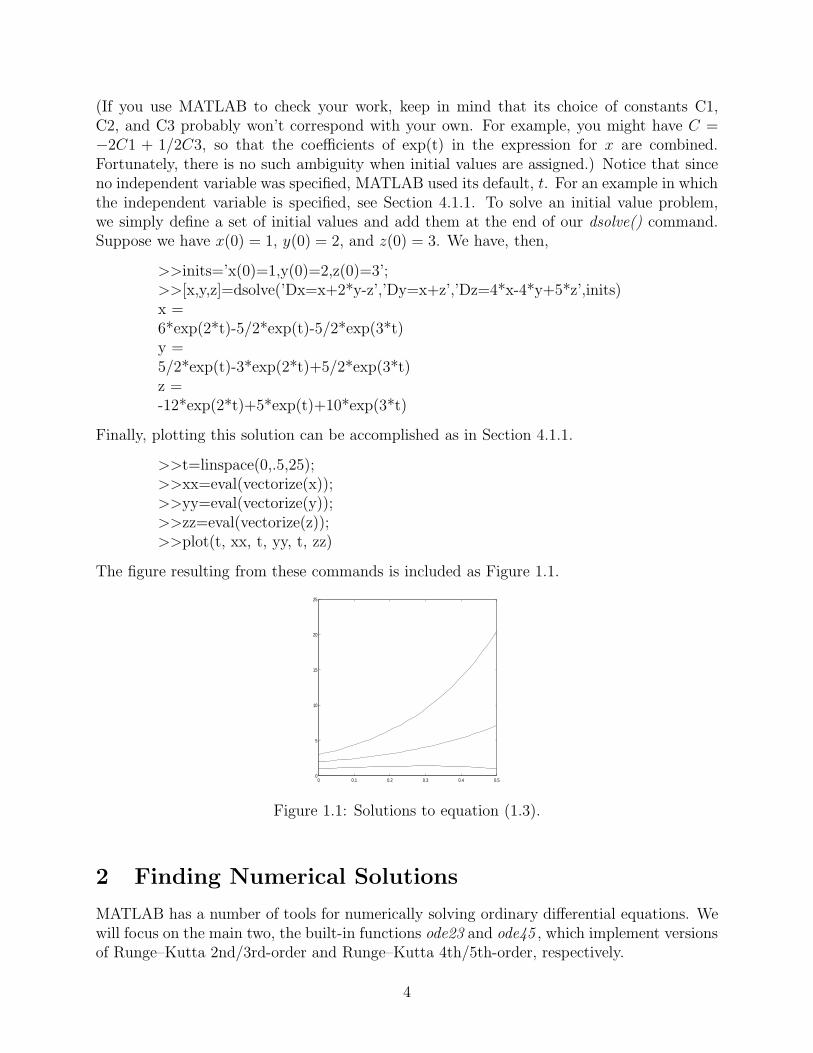
(If you use MATLAB to check your work, keep in mind that its choice of constants C1,C2, and C3 probably won’t correspond with your own. For example, you might have C =−2C1 + 1/2C3, so that the coefficients of exp(t) in the expression for x are combined.Fortunately, there is no such ambiguity when initial values are assigned.) Notice that sinceno independent variable was specified, MATLAB used its default, t. For an example in whichthe independent variable is specified, see Section 4.1.1. To solve an initial value problem,we simply define a set of initial values and add them at the end of our dsolve() command.Suppose we have x(0) = 1, y(0) = 2, and z(0) = 3. We have, then,

>>inits=’x(0)=1,y(0)=2,z(0)=3’;>>[x,y,z]=dsolve(’Dx=x+2*y-z’,’Dy=x+z’,’Dz=4*x-4*y+5*z’,inits)x =6*exp(2*t)-5/2*exp(t)-5/2*exp(3*t)y =5/2*exp(t)-3*exp(2*t)+5/2*exp(3*t)z =-12*exp(2*t)+5*exp(t)+10*exp(3*t)

Finally, plotting this solution can be accomplished as in Section 4.1.1.

>>t=linspace(0,.5,25);>>xx=eval(vectorize(x));>>yy=eval(vectorize(y));>>zz=eval(vectorize(z));>>plot(t, xx, t, yy, t, zz)

The figure resulting from these commands is included as Figure 1.1.

0 0.1 0.2 0.3 0.4 0.50

5

10

15

20

25

Figure 1.1: Solutions to equation (1.3).

2 Finding Numerical Solutions

MATLAB has a number of tools for numerically solving ordinary differential equations. Wewill focus on the main two, the built-in functions ode23 and ode45 , which implement versionsof Runge–Kutta 2nd/3rd-order and Runge–Kutta 4th/5th-order, respectively.

4

2.1 First-Order Equations with Inline Functions

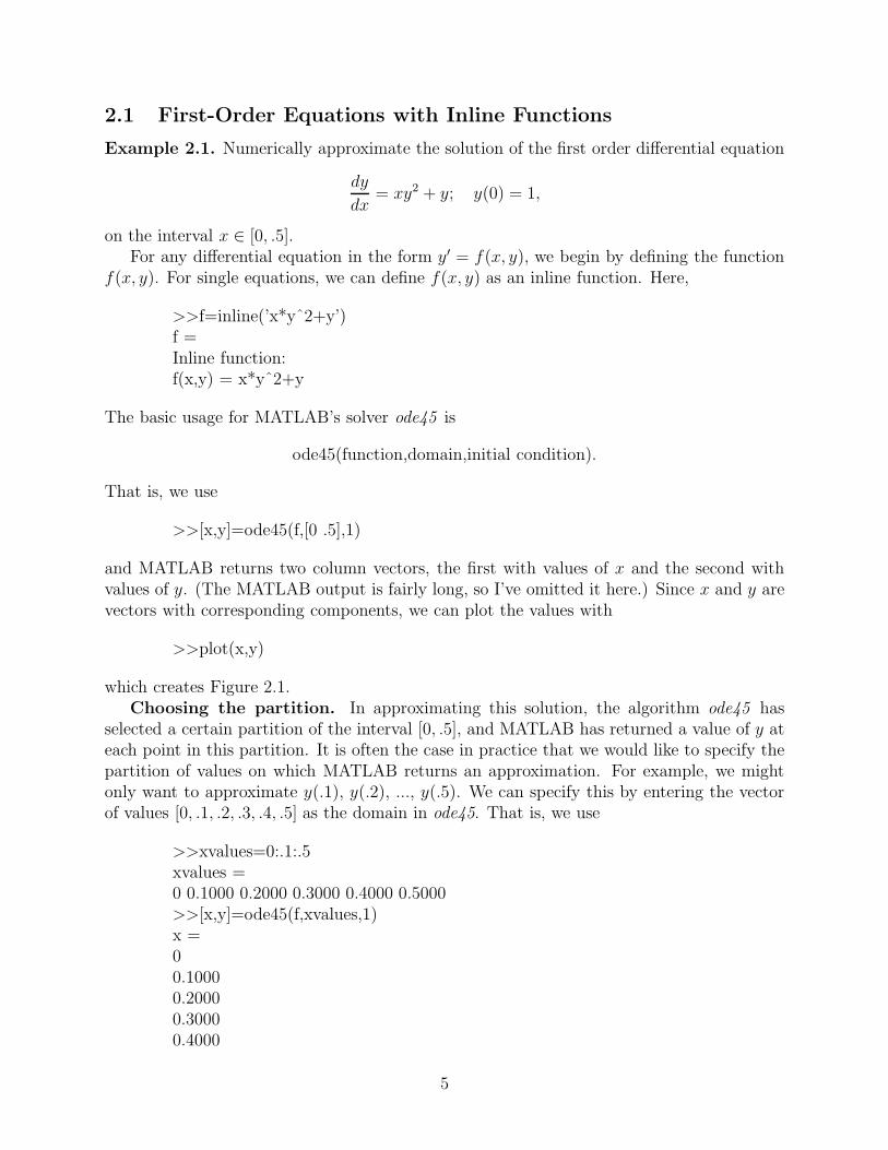
Example 2.1. Numerically approximate the solution of the first order differential equation

dy

dx= xy2 + y; y(0) = 1,

on the interval x ∈ [0, .5].For any differential equation in the form y′ = f(x, y), we begin by defining the function

f(x, y). For single equations, we can define f(x, y) as an inline function. Here,

>>f=inline(’x*yˆ2+y’)f =Inline function:f(x,y) = x*yˆ2+y

The basic usage for MATLAB’s solver ode45 is

ode45(function,domain,initial condition).

That is, we use

>>[x,y]=ode45(f,[0 .5],1)

and MATLAB returns two column vectors, the first with values of x and the second withvalues of y. (The MATLAB output is fairly long, so I’ve omitted it here.) Since x and y arevectors with corresponding components, we can plot the values with

>>plot(x,y)

which creates Figure 2.1.Choosing the partition. In approximating this solution, the algorithm ode45 has

selected a certain partition of the interval [0, .5], and MATLAB has returned a value of y ateach point in this partition. It is often the case in practice that we would like to specify thepartition of values on which MATLAB returns an approximation. For example, we mightonly want to approximate y(.1), y(.2), ..., y(.5). We can specify this by entering the vectorof values [0, .1, .2, .3, .4, .5] as the domain in ode45. That is, we use

>>xvalues=0:.1:.5xvalues =0 0.1000 0.2000 0.3000 0.4000 0.5000>>[x,y]=ode45(f,xvalues,1)x =00.10000.20000.30000.4000

5

0 0.1 0.2 0.3 0.4 0.5 0.6 0.71

1.1

1.2

1.3

1.4

1.5

1.6

1.7

1.8

1.9

2

Figure 2.1: Plot of the solution to y′ = xy2 + y, with y(0) = 1.

0.5000y =1.00001.11111.25001.42861.66672.0000

It is important to point out here that MATLAB continues to use roughly the same partitionof values that it originally chose; the only thing that has changed is the values at which it isprinting a solution. In this way, no accuracy is lost.

Options. Several options are available for MATLAB’s ode45 solver, giving the user lim-ited control over the algorithm. Two important options are relative and absolute tolerance,respecively RelTol and AbsTol in MATLAB. At each step of the ode45 algorithm, an erroris approximated for that step. If yk is the approximation of y(xk) at step k, and ek is theapproximate error at this step, then MATLAB chooses its partition to insure

ek ≤ max(RelTol ∗ yk, AbsTol),

where the default values are RelTol = .001 and AbsTol = .000001. As an example for whenwe might want to change these values, observe that if yk becomes large, then the error ek

will be allowed to grow quite large. In this case, we increase the value of RelTol. For theequation y′ = xy2 + y, with y(0) = 1, the values of y get quite large as x nears 1. In fact,with the default error tolerances, we find that the command

>>[x,y]=ode45(f,[0,1],1);

6

leads to an error message, caused by the fact that the values of y are getting too large as xnears 1. (Note at the top of the column vector for y that it is multipled by 1014.) In orderto fix this problem, we choose a smaller value for RelTol.

>>options=odeset(’RelTol’,1e-10);>>[x,y]=ode45(f,[0,1],1,options);>>max(y)ans =2.425060345544448e+07

In addition to employing the option command, I’ve computed the maximum value of y(x)to show that it is indeed quite large, though not as large as suggested by the previouscalculation. △

2.2 First Order Equations with M-files

Alternatively, we can solve the same ODE as in Example 2.1 by first defining f(x, y) as anM-file firstode.m.

function yprime = firstode(x,y);% FIRSTODE: Computes yprime = x*yˆ2+yyprime = x*yˆ2 + y;

In this case, we only require one change in the ode45 command: we must use a pointer @to indicate the M-file. That is, we use the following commands.

>>xspan = [0,.5];>>y0 = 1;>>[x,y]=ode23(@firstode,xspan,y0);>>x

2.3 Systems of ODE

Solving a system of ODE in MATLAB is quite similar to solving a single equation, thoughsince a system of equations cannot be defined as an inline function we must define it as anM-file.

Example 2.2. Solve the system of Lorenz equations,2

dx

dt= − σx + σy

dy

dt=ρx − y − xz

dz

dt= − βz + xy, (2.1)

2The Lorenz equations have some properties of equations arising in atmospherics. Solutions of the Lorenz

equations have long served as an example for chaotic behavior.

7

where for the purposes of this example, we will take σ = 10, β = 8/3, and ρ = 28, as well asx(0) = −8, y(0) = 8, and z(0) = 27. The MATLAB M-file containing the Lorenz equationsappears below.

function xprime = lorenz(t,x);%LORENZ: Computes the derivatives involved in solving the%Lorenz equations.sig=10;beta=8/3;rho=28;xprime=[-sig*x(1) + sig*x(2); rho*x(1) - x(2) - x(1)*x(3); -beta*x(3) + x(1)*x(2)];

Observe that x is stored as x(1), y is stored as x(2), and z as stored as x(3). Additionally,xprime is a column vector, as is evident from the semicolon following the first appearance ofx(2). If in the Command Window, we type

>>x0=[-8 8 27];>>tspan=[0,20];>>[t,x]=ode45(@lorenz,tspan,x0)

Though not given here, the output for this last command consists of a column of timesfollowed by a matrix with three columns, the first of which corresponds with values of xat the associated times, and similarly for the second and third columns for y and z. Thematrix has been denoted x in the statement calling ode45, and in general any coordinate ofthe matrix can be specified as x(m, n), where m denotes the row and n denotes the column.What we will be most interested in is referring to the columns of x, which correspond withvalues of the components of the system. Along these lines, we can denote all rows or allcolumns by a colon :. For example, x(:,1) refers to all rows in the first column of the matrixx; that is, it refers to all values of our original x component. Using this information, we caneasily plot the Lorenz strange attractor, which is a plot of z versus x:

>>plot(x(:,1),x(:,3))

See Figure 2.2.Of course, we can also plot each component of the solution as a function of t, and one

useful way to do this is to stack the results. We can create Figure 2.3 with the followingMATLAB code.

>>subplot(3,1,1)>>plot(t,x(:,1))>>subplot(3,1,2)>>plot(t,x(:,2))>>subplot(3,1,3)>>plot(t,x(:,3))

8

−20 −15 −10 −5 0 5 10 15 205

10

15

20

25

30

35

40

45The Lorenz Strange Attractor

x

y

Figure 2.2: The Lorenz Strange Attractor

0 2 4 6 8 10 12 14 16 18 20−20

−10

0

10

20Components for the Lorenz Equations

0 2 4 6 8 10 12 14 16 18 20−50

0

50

0 2 4 6 8 10 12 14 16 18 200

20

40

60

Figure 2.3: Plot of coordinates for the Lorenz equations as a function of t.

9

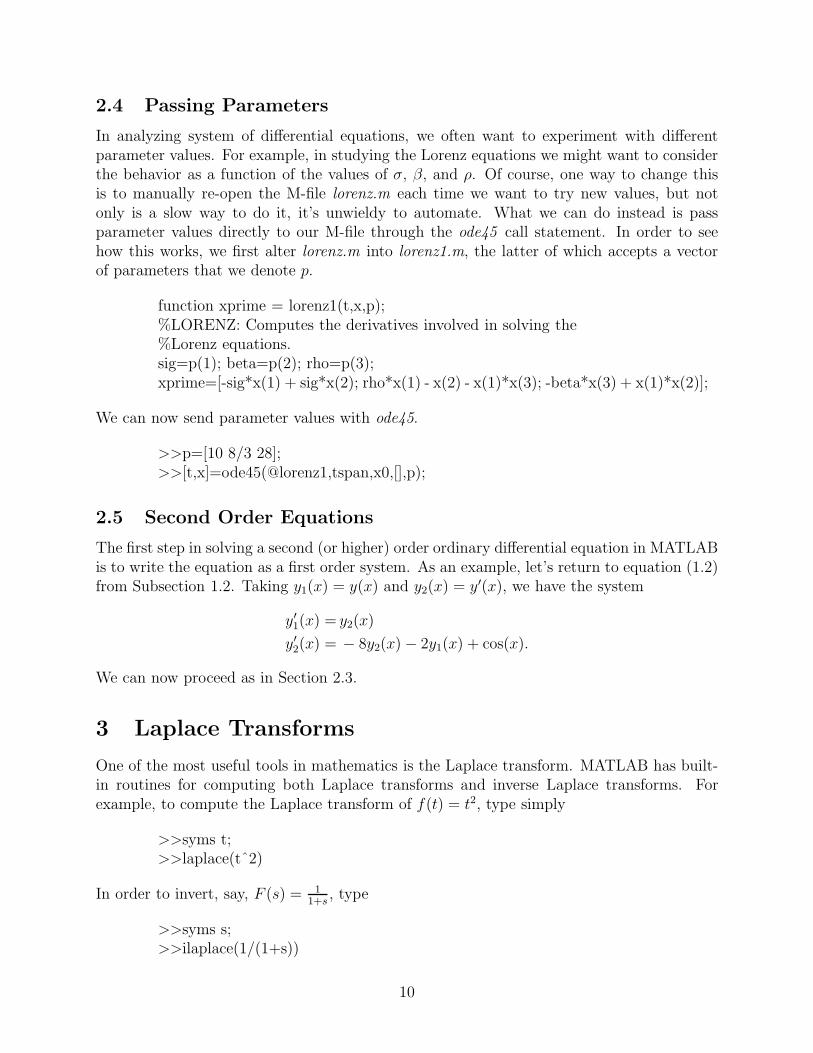
2.4 Passing Parameters

In analyzing system of differential equations, we often want to experiment with differentparameter values. For example, in studying the Lorenz equations we might want to considerthe behavior as a function of the values of σ, β, and ρ. Of course, one way to change thisis to manually re-open the M-file lorenz.m each time we want to try new values, but notonly is a slow way to do it, it’s unwieldy to automate. What we can do instead is passparameter values directly to our M-file through the ode45 call statement. In order to seehow this works, we first alter lorenz.m into lorenz1.m, the latter of which accepts a vectorof parameters that we denote p.

function xprime = lorenz1(t,x,p);%LORENZ: Computes the derivatives involved in solving the%Lorenz equations.sig=p(1); beta=p(2); rho=p(3);xprime=[-sig*x(1) + sig*x(2); rho*x(1) - x(2) - x(1)*x(3); -beta*x(3) + x(1)*x(2)];

We can now send parameter values with ode45.

>>p=[10 8/3 28];>>[t,x]=ode45(@lorenz1,tspan,x0,[],p);

2.5 Second Order Equations

The first step in solving a second (or higher) order ordinary differential equation in MATLABis to write the equation as a first order system. As an example, let’s return to equation (1.2)from Subsection 1.2. Taking y1(x) = y(x) and y2(x) = y′(x), we have the system

y′

1(x) = y2(x)

y′

2(x) = − 8y2(x) − 2y1(x) + cos(x).

We can now proceed as in Section 2.3.

3 Laplace Transforms

One of the most useful tools in mathematics is the Laplace transform. MATLAB has built-in routines for computing both Laplace transforms and inverse Laplace transforms. Forexample, to compute the Laplace transform of f(t) = t2, type simply

>>syms t;>>laplace(tˆ2)

In order to invert, say, F (s) = 11+s

, type

>>syms s;>>ilaplace(1/(1+s))

10

4 Boundary Value Problems

For various reasons of arguable merit most introductory courses on ordinary differentialequations focus primarily on initial value problems (IVP’s). Another class of ODE’s thatoften arise in applications are boundary value problems (BVP’s). Consider, for example, thedifferential equation

y′′ − 3y′ + 2y =0

y(0) = 0

y(1) = 10,

where our conditions y(0) = 0 and y(1) = 10 are specified on the boundary of the interval ofinterest x ∈ [0, 1]. (Though our solution will typically extend beyond this interval, the mostcommon scenario in boundary value problems is the case in which we are only interested invalues of the independent variable between the specified endpoints.) The first step in solvingthis type of equation is to write it as a first order system with y1 = y and y2 = y′, for whichwe have

y′

1 = y2

y′

2 = − 2y1 + 3y2.

We record this system in the M-file bvpexample.m.

function yprime = bvpexample(t,y)%BVPEXAMPLE: Differential equation for boundary value%problem example.yprime=[y(2); -2*y(1)+3*y(2)];

Next, we write the boundary conditions as the M-file bc.m, which records boudary residues.

function res=bc(y0,y1)%BC: Evaluates the residue of the boundary conditionres=[y0(1);y1(1)-10];

By residue, we mean the left-hand side of the boundary condition once it has been set to 0.In this case, the second boundary condition is y(1) = 10, so its residue is y(1) − 10, whichis recorded in the second component of the vector that bc.m returns. The variables y0 andy1 represent the solution at x = 0 and at x = 1 respectively, while the 1 in parenthesesindicates the first component of the vector. In the event that the second boundary conditionwas y′(1) = 10, we would replace y1(1)− 10 with y1(2) − 10.

We are now in a position to begin solving the boundary value problem. In the followingcode, we first specify a grid of x values for MATLAB to solve on and an initial guess forthe vector that would be given for an initial value problem [y(0), y′(0)]. (Of course, y(0) isknown, but y′(0) must be a guess. Loosely speaking, MATLAB will solve a family of initialvalue problems, searching for one for which the boundary conditions are met.) We solve theboundary value problem with MATLAB’s built-in solver bvp4c.

11

>>sol=bvpinit(linspace(0,1,25),[0 1]);>>sol=bvp4c(@bvpexample,@bc,sol);>>sol.xans =Columns 1 through 90 0.0417 0.0833 0.1250 0.1667 0.2083 0.2500 0.2917 0.3333Columns 10 through 180.3750 0.4167 0.4583 0.5000 0.5417 0.5833 0.6250 0.6667 0.7083Columns 19 through 250.7500 0.7917 0.8333 0.8750 0.9167 0.9583 1.0000>>sol.yans =Columns 1 through 90 0.0950 0.2022 0.3230 0.4587 0.6108 0.7808 0.9706 1.18212.1410 2.4220 2.7315 3.0721 3.4467 3.8584 4.3106 4.8072 5.3521Columns 10 through 181.4173 1.6787 1.9686 2.2899 2.6455 3.0386 3.4728 3.9521 4.48055.9497 6.6050 7.3230 8.1096 8.9710 9.9138 10.9455 12.0742 13.3084Columns 19 through 255.0627 5.7037 6.4090 7.1845 8.0367 8.9726 9.999914.6578 16.1327 17.7443 19.5049 21.4277 23.5274 25.8196

We observe that in this case MATLAB returns the solution as a structure whose first compo-nent sol.x simply contains the x values we specified. The second component of the structuresol is sol.y, which is a matrix containing as its first row values of y(x) at the x grid pointswe specified, and as its second row the corresponding values of y′(x).

5 Event Location

Typically, the ODE solvers in MATLAB terminate after solving the ODE over a specifieddomain of the independent variable (the range we have referred to above as xspan or tspan).In applications, however, we often would like to stop the solution at a particular value of thedependent variable (for example, when an object fired from the ground reaches its maximumheight or when a population crosses some threshhold value). As an example, suppose wewould like to determine the period of the pendulum from Example 3.1. Since we do not knowthe appropriate time interval (in fact, that’s what we’re trying to determine), we would like tospecify that MATLAB solve the equation until the pendulum swings through some specifiedfraction of its complete cycle and to give the time this took. In our case, we will record thetime it takes the pendulum to reach the bottom of its arc, and multiply this by 4 to arriveat the pendulum’s period. (In this way, the event is independent of the pendulum’s initialconditions.) Our pendulum equation

d2θ

dt2= −

g

lsin θ

12

is stored in pendode.m with l = 1 (see Example 3.1). In addition to this file, we write anevents file pendevent.m that specifies the event we are looking for.

function [lookfor stop direction]=pendevent(t,x)%PENDEVENT: MATLAB function M-file that contains the event%that our pendulum reaches its center point from the rightlookfor = x(1) ; %Searches for this expression set to 0stop = 1; %Stop when event is locateddirection = -1; %Specifiy direction of motion at event

In pendevent.m, the line lookfor=x(1) specifies that MATLAB should look for the eventx(1) = 0 (that is, x(t) = 0). (If we wanted to look for the event x(t) = 1, we would uselookfor=x(1)-1.) The line stop=1 instructs MATLAB to stop solving when the event islocated, and the command direction=-1 instructs MATLAB to only accept events for whichx(2) (that is, x′) is negative (if the pendulum starts to the right of center, it will be movingin the negative direction the first time it reaches the center point).

We can now solve the ODE up until the time our pendulum reaches the center point withthe following commands issued in the Command Window:

>>options=odeset(’Events’,@pendevent);>>x0=[pi/4 0];>>[t, x, te, xe, ie]=ode45(@pendode, [0, 10], x0, options);>>tete =0.5215>>xexe =-0.0000 -2.3981

Here, x0 is a vector of initial data, for which we have chosen that the pendulum begin withangle π/4 and with no initial velocity. The command ode45() returns a vector of times t, amatrix of dependent variables x, the time at which the event occurred, te, and the valuesof x when the event occurred, xe. In the event that a vector of events is specified, indexvector ie describes which event has occured in each instance. Here, only a single event hasbeen specified, so ie=1. In this case, we see that the event occurred at time t = .5215, andconsequently the period is P = 2.086 (within numerical errors). Though the exact period ofthe pendulum is difficult to analyze numerically, it is not difficult to show through the smallangle approximation sin θ ∼= θ that for θ small the period of the pendulum is approximately

P = 2π√

lg, which in our case gives P = 2.001. (While the small angle approximation gives

a period independent of θ, the period of a pendulum does depend on θ.)In order to better understand this index ie, let’s verify that the time is the same for each

quarter swing. That is, let’s record the times at which θ = 0 and additionally the times atwhich θ′ = 0 and look at the times between them. In this case, pendevent.m is replaced bypendevent1.m.

13

function [lookfor stop direction]=pendevent1(t,x)%PENDEVENT1: MATLAB function M-file that contains the event%that our pendulum returns to its original postion pi/4lookfor = [x(1);x(2)]; %Searches for this expression set to 0stop = [0;0]; %Do not stop when event is locateddirection = [0;0]; %Either direction accepted

In this case, we are looking for two different events, and so the variables in pendevent1.mare vectors with two components, each corresponding with an event. In this case, we do notstop after either event, and we do not specify a direction. In the Command Window, wehave the following.

>>options=odeset(’Events’,@pendevent1);>>x0=[pi/4 0];>>[t, x, te, xe, ie]=ode45(@pendode,[0 2],x0,options);>>tete =0.00000.52161.04311.5646>>xexe =0.7854 -0.0000-0.0000 -2.3972-0.7853 0.00000.0000 2.3970>>ieie =2121

We see that over a time interval [0, 2] the event times are approximately 0, .5216, 1.0431,and 1.5646. Looking at the matrix xe, for which the first value in each row is an angularposition and the second is an angular velocity, we see that the first event correponds with thestarting position, the second event corresponds with the pendulum’s hanging straight down,the third event corresponds with the pendulum’s having swung entirely to the opposite side,and the fourth event corresponds with the pendulum’s hanging straight down on its returntrip. It’s now clear how ie works: it is 2 when the second event we specified occurs and 1when the first event we specified occurs.

14

6 Numerical Methods

Though we can solve ODE on MATLAB without any knowledge of the numerical methodsit employs, it’s often useful to understand the basic underlying principles. In this section wewill use Taylor’s Theorem to derive methods for approximating the solution to a differentialequation.

6.1 Euler’s Method

Consider the general first order differential equation

dy

dx= f(x, y); y(x0) = y0, (6.1)

and suppose we would like to solve this equation on the interval of x-values [x0, xn]. Our goalwill be to approximate the value of the solution y(x) at each of the x values in a partitionP = [x0, x1, x2, ..., xn]. Since y(x0) is given, the first value we need to estimate is y(x1). ByTaylor’s Theorem, we can write

y(x1) = y(x0) + y′(x0)(x1 − x0) +y′(c)

2(x1 − x0)

2,

where c ∈ (x0, x1). Observing from our equation that y′(x0) = f(x0, y(x0)), we have

y(x1) = y(x0) + f(x0, y(x0))(x1 − x0) +y′(c)

2(x1 − x0)

2.

If our partition P has small subintervals, then x1 − x0 will be small, and we can regard thesmaller quantity y′(c)

2(x1 − x0)

2 as an error term. That is, we have

y(x1) ≈ y(x0) + f(x0, y(x0))(x1 − x0). (6.2)

We can now compute y(x2) in a similar manner by using Taylor’s Theorem to write

y(x2) = y(x1) + y′(x1)(x2 − x1) +y′(c)

2(x2 − x1)

2.

Again, we have from our equation that y′(x1) = f(x1, y(x1)), and so

y(x2) = y(x1) + f(x1, y(x1))(x2 − x1) +y′(c)

2(x2 − x1)

2.

If we drop the term y′(c)2

(x2 − x1)2 as an error, then we have

y(x2) ≈ y(x1) + f(x1, y(x1))(x2 − x1),

where the value y(x1) required here can be approximate by the value from (6.2). Moregenerally, for any k = 1, 2, ..., n − 1 we can approximate y(xk+1) from the relation

y(xk+1) ≈ y(xk) + f(xk, y(xk))(xk+1 − xk),

15

where y(xk) will be known from the previous calculation. As with methods of numericalintegration, it is customary in practice to take our partition to consist of subintervals ofequal width,

(xk+1 − xk) = △x =xn − x0

n.

(In the study of numerical methods for differential equations, this quantity is often denotedh.) In this case, we have the general relationship

y(xk+1) ≈ y(xk) + f(xk, y(xk))△x.

If we let the values y0, y1, ..., yn denote our approximations for y at the points x0, x1, ..., xn

(that is, y0 = y(x0), y1 ≈ y(x1), etc.), then we can approximate y(x) on the partition P byiteratively computing

yk+1 = yk + f(xk, yk)△x. (6.3)

Example 6.1. Use Euler’s method (6.3) with n = 10 to solve the differential equation

dy

dx= sin(xy); y(0) = π,

on the interval [0, 1]. We will carry out the first few iterations in detail, and then we willwrite a MATLAB M-file to carry it out in its entirety. First, the initial value y(0) = π givesus the values x0 = 0 and y0 = π. If our partition is composed of subintervals of equal width,then x1 = △x = 1

10= .1, and according to (6.3)

y1 = y0 + sin(x0y0)△x = π + sin(0).1 = π.

We now have the point (x1, y1) = (.1, π), and we can use this and 6.3 to compute

y2 = y1 + sin(x1y1)△x = π + sin(.1π)(.1) = 3.1725.

We now have (x2, y2) = (.2, 3.1725), and we can use this to compute

y3 = y2 + sin(x2y2)△x = 3.1725 + sin(.2(3.1725))(.1) = 3.2318.

More generally, we can use the M-file euler.m.

function [xvalues, yvalues] = euler(f,x0,xn,y0,n)%EULER: MATLAB function M-file that solve the%ODE y’=f, y(x0)=y0 on [x0,y0] using a partition%with n equally spaced subintervalsdx = (xn-x0)/n;x(1) = x0;y(1) = y0;for k=1:nx(k+1)=x(k) + dx;y(k+1)= y(k) + f(x(k),y(k))*dx;endxvalues = x’;yvalues = y’;

16

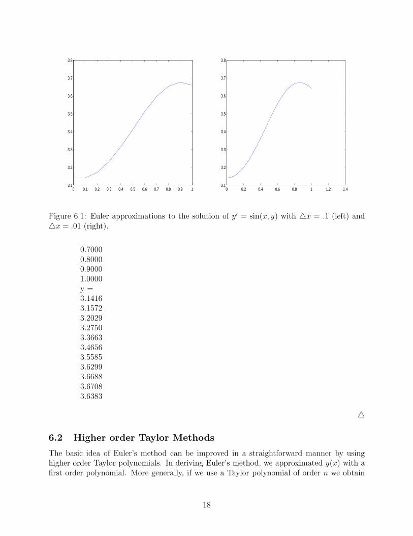
We can implement this file with the following code, which creates Figure 6.1.

>>f=inline(’sin(x*y)’)f =Inline function:f(x,y) = sin(x*y)>>[x,y]=euler(f,0,1,pi,10)x =00.10000.20000.30000.40000.50000.60000.70000.80000.90001.0000y =3.14163.14163.17253.23183.31423.41123.51033.59633.65483.67643.6598>>plot(x,y)>>[x,y]=euler(f,0,1,pi,100);>>plot(x,y)

For comparison, the exact values to four decimal places are given below.

x =00.10000.20000.30000.40000.50000.6000

17

0 0.1 0.2 0.3 0.4 0.5 0.6 0.7 0.8 0.9 13.1

3.2

3.3

3.4

3.5

3.6

3.7

3.8

0 0.2 0.4 0.6 0.8 1 1.2 1.43.1

3.2

3.3

3.4

3.5

3.6

3.7

3.8

Figure 6.1: Euler approximations to the solution of y′ = sin(x, y) with △x = .1 (left) and△x = .01 (right).

0.70000.80000.90001.0000y =3.14163.15723.20293.27503.36633.46563.55853.62993.66883.67083.6383

△

6.2 Higher order Taylor Methods

The basic idea of Euler’s method can be improved in a straightforward manner by usinghigher order Taylor polynomials. In deriving Euler’s method, we approximated y(x) with afirst order polynomial. More generally, if we use a Taylor polynomial of order n we obtain

18

the Taylor method of order n. In order to see how this is done, we will derive the Taylormethod of order 2. (Euler’s method is the Taylor method of order 1.)

Again letting P = [x0, x1, ..., xn] denote a partition of the interval [x0, xn] on which wewould like to solve (6.1), our starting point for the Taylor method of order 2 is to write downthe Taylor polynomial of order 2 (with remainder) for y(xk+1) about the point xk. That is,according to Taylor’s theorem,

y(xk+1) = y(xk) + y′(xk)(xk+1 − xk) +y′′(xk)

2(xk+1 − xk)

2 +y′′′(c)

3!(xk+1 − xk)

3,

where c ∈ (xk, xk+1). As with Euler’s method, we drop off the error term (which is nowsmaller), and our approximation is

y(xk+1) ≈ y(xk) + y′(xk)(xk+1 − xk) +y′′(xk)

2(xk+1 − xk)

2.

We already know from our derivation of Euler’s method that y′(xk) can be replaced withf(xk, y(xk)). In addition to this, we now need an expression for y′′(xk). We can obtain thisby differentiating the original equation y′(x) = f(x, y(x)). That is,

y′′(x) =d

dxy′(x) =

d

dxf(x, y(x)) =

∂f

∂x(x, y(x)) +

∂f

∂y(x, y(x))

dy

dx,

where the last equality follows from a generalization of the chain rule to functions of twovariables (see Section 10.5.1 of the course text). From this last expression, we see that

y′′(xk) =∂f

∂x(xk, y(xk)) +

∂f

∂y(xk, y(xk))y

′(xk) =∂f

∂x(xk, y(xk)) +

∂f

∂y(xk, y(xk))f(xk, y(xk)).

Replacing y′′(xk) with the right-hand side of this last expression, and replacing y′(xk) withf(xk, y(xk)), we conclude

y(xk+1) ≈ y(xk) + f(xk, y(xk))(xk+1 − xk)

+[∂f

∂x(xk, y(xk)) +

∂f

∂y(xk, y(xk))f(xk, y(xk))

](xk+1 − xk)2

2.

If we take subintervals of equal width △x = (xk+1 − xk), this becomes

y(xk+1) ≈ y(xk) + f(xk, y(xk))△x

+[∂f

∂x(xk, y(xk)) +

∂f

∂y(xk, y(xk))f(xk, y(xk))

]

△x2

2.

Example 6.2. Use the Taylor method of order 2 with n = 10 to solve the differentialequation

dy

dx= sin(xy); y(0) = π,

on the interval [0, 1].

19

We will carry out the first few iterations by hand and leave the rest as an exercise. Tobegin, we observe that

f(x, y) = sin(xy)

∂f

∂x(x, y) = y cos(xy)

∂f

∂y(x, y) = x cos(xy).

If we let yk denote an approximation for y(xk), the Taylor method of order 2 becomes

yk+1 = yk + sin(xkyk)(.1)

+[

yk cos(xkyk) + xk cos(xkyk) sin(xkyk)](.1)2

2.

Beginning with the point (x0, y0) = (0, π), we compute

y1 = π + π(.005) = 3.1573,

which is closer to the correct value of 3.1572 than was the approximation of Euler’s method.We can now use the point (x1, y1) = (.1, 3.1573) to compute

y2 =3.1573 + sin(.1 · 3.1573)(.1)

+[

3.1573 cos(.1 · 3.1573) + .1 cos(.1 · 3.1573) sin(.1 · 3.1573)](.1)2

2=3.2035,

which again is closer to the correct value than was the y2 approximation for Euler’s method.△

7 Advanced ODE Solvers

In addition to the ODE solvers ode23 and ode45, which are both based on the Runge–Kuttascheme, MATLAB has several additional solvers, listed below along with MATLAB’s help-filesuggestions regarding when to use them.

• Multipstep solvers

– ode113. If using stringent error tolerances or solving a computationally intensiveODE file.

• Stiff problems (see discussion below)

– ode15s. If ode45 is slow because the problem is stiff.

– ode23s. If using crude error tolerances to solve stiff systems and the mass matrixis constant.

– ode23t. If the problem is only moderately stiff and you need a solution withoutnumerical damping.

– ode23tb. If using crude error tolerances to solve stiff systems.

20

7.1 Stiff ODE

By a stiff ODE we mean an ODE for which numerical errors compound dramatically overtime. For example, consider the ODE

y′ = −100y + 100t + 1; y(0) = 1.

Since the dependent variable, y, in the equation is multiplied by 100, small errors in ourapproximation will tend to become magnified. In general, we must take considerably smallersteps in time to solve stiff ODE, and this can lengthen the time to solution dramatically.Often, solutions can be computed more efficiently using one of the solvers designed for stiffproblems.

21

Index

boundary value problems, 11

dsolve, 2

eval, 2event location, 12

inverse laplace, 10

laplace, 10Laplace transforms, 10

ode, 4ode113(), 20ode15s(), 20ode23s(), 20ode23t(), 20ode23tb(), 20

stiff ODE, 21

vectorize(), 2

22