Systems of ODE and MatLab - Home | College of...
76
Introduction to ODE Systems of ODE and MatLab James K. Peterson Department of Biological Sciences and Department of Mathematical Sciences Clemson University June 14, 2017
-
Upload
truonghanh -
Category
Documents
-
view
217 -
download
3
Transcript of Systems of ODE and MatLab - Home | College of...
Introduction to ODE
Systems of ODE and MatLab
James K. Peterson
Department of Biological Sciences and Department of Mathematical SciencesClemson University
June 14, 2017

Introduction to ODE
Outline
1 Systems of ODEs
2 Adding External Input Functions
3 Linear Second Order Problems As Systems
4 Linear Systems Numerically
5 An Attempt At An Automated Phase Plane Plot
6 Further Automation! Eigenvalues in MatLab

Introduction to ODE
Abstract
This lecture is going to discuss using numerical methods for solvingODE systems.

Introduction to ODE
Systems of ODEs
We now want to learn how to solve systems of differentialequations. A typical system is the following
x ′(t) = f (t, x(t), y(t)) (1)
y ′(t) = g(t, x(t), y(t)) (2)
x(t0) = x0; y(t0) = y0 (3)
where x and y are our variables of interest which mightrepresent populations to two competing species or otherquantities of biological interest.
The system starts at time t0 (which for us is usually 0) andwe specify the values the variables x and y start at as x0 andy0 respectively. The functions f and g are “nice” meaningthat as functions of three arguments (t, x , y) they do not havejumps and corners. The exact nature of “nice” here is a bitbeyond our ability to discuss in this introductory course, so wewill leave it at that.

Introduction to ODE
Systems of ODEs
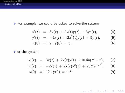
For example, we could be asked to solve the system
x ′(t) = 3x(t) + 2x(t)y(t) − 3y2(t), (4)
y ′(t) = −2x(t) + 2x2(t)y(t) + 5y(t), (5)
x(0) = 2; y(0) = 3. (6)
or the system
x ′(t) = 3x(t) + 2x(t)y(t) + 10 sin(t2 + 5), (7)
y ′(t) = −2x(t) + 2x(t)y2(t) + 20t3e−2t2, (8)
x(0) = 12; y(0) = −5. (9)
Introduction to ODE
Systems of ODEs
For example, we could be asked to solve the system
x ′(t) = 3x(t) + 2x(t)y(t) − 3y2(t), (4)
y ′(t) = −2x(t) + 2x2(t)y(t) + 5y(t), (5)
x(0) = 2; y(0) = 3. (6)
or the system
x ′(t) = 3x(t) + 2x(t)y(t) + 10 sin(t2 + 5), (7)
y ′(t) = −2x(t) + 2x(t)y2(t) + 20t3e−2t2, (8)
x(0) = 12; y(0) = −5. (9)

Introduction to ODE
Systems of ODEs
The functions f and g in these examples are not linear in thevariables x and y ; hence the system Equation 4 and Equation5 and system Equation 7 and Equation 8 are what are called anonlinear systems. In general, arbitrary functions of time, φand ψ to the model giving
x ′(t) = 3x(t) + 2x(t)y(t) − 3y2(t) + φ(t), (10)
y ′(t) = −2x(t) + 2x2(t)y(t) + 5y(t) + ψ(t), (11)
x(0) = 2; y(0) = 3. (12)
The functions φ and ψ are what we could call data functions.For example, if φ(t) = sin(t) and ψ(t) = te−t , the systemEquation 10 and Equation 11 would become
x ′(t) = 3x(t) + 2x(t)y(t) − 3y2(t) + sin(t),
y ′(t) = −2x(t) + 2x2(t)y(t) + 5y(t) + te−t ,
x(0) = 2; y(0) = 3.

Introduction to ODE
Systems of ODEs
The functions f and g would then become
f (t, x , y) = 3x + 2xy − 3y2 + sin(t)
g(t, x , y) = −2x + 2x2y + 5y + te−t
How do we solve such a system of differential equations?There are some things we can do if the functions f and g arelinear in x and y , but many times we will be forced to look atthe solutions using numerical techniques. We explored how tosolve first order equations already and we will now adapt thetools developed earlier to systems of differential equations.

Introduction to ODE
Linear Second Order Problems As Systems
Now let’s consider how to adapt our previous code to handlethese systems of differential equations. We will begin with thelinear second order problems because we know how to dothose already. First, let’s consider a general second orderlinear problem.
a u′′(t) + b u′(t) + c u(t) = g(t), u(0) = u0, u′(0) = u1
where we assume a is not zero, so that we really do have asecond order problem!
As usual, we let the vector x be given by
x(t) =
[x1(t)x2(t)
]=
[u(t)u′(t)
]Then,
x ′1(t) = u′(t) = x2(t),
x ′2(t) = u′′(t) = −(c/a)u(t) − (b/a)u′(t) + (1/a) g(t)

Introduction to ODE
Linear Second Order Problems As Systems
Now let’s consider how to adapt our previous code to handlethese systems of differential equations. We will begin with thelinear second order problems because we know how to dothose already. First, let’s consider a general second orderlinear problem.
a u′′(t) + b u′(t) + c u(t) = g(t), u(0) = u0, u′(0) = u1
where we assume a is not zero, so that we really do have asecond order problem!As usual, we let the vector x be given by
x(t) =
[x1(t)x2(t)
]=
[u(t)u′(t)
]Then,
x ′1(t) = u′(t) = x2(t),
x ′2(t) = u′′(t) = −(c/a)u(t) − (b/a)u′(t) + (1/a) g(t)

Introduction to ODE
Linear Second Order Problems As Systems
We then convert the above into the matrix - vector system
x ′(t) =
[x ′1(t)x ′2(t)
]=
[0 1
−(c/a) −(b/a)
] [x1(t)x2(t)
]+
[0
(1/a) g(t)
]
Also, note that
x(0) =
[x1(0)x2(0)
]=
[u(0)u′(0)
]=
[u0u1
]= x0.
For our purposes of using MatLab, we need to write this interms of vectors. We have[
x ′1(t)x ′2(t)
]=
[x2
−(c/a) x1 − (b/a) x2 + (1/a) g(t)
]Now let the dynamics vector f be defined by
f =
[f1f2
]=
[x2
−(c/a) x1 − (b/a) x2 + (1/a) g(t)
]

Introduction to ODE
Linear Second Order Problems As Systems
We then convert the above into the matrix - vector system
x ′(t) =
[x ′1(t)x ′2(t)
]=
[0 1
−(c/a) −(b/a)
] [x1(t)x2(t)
]+
[0
(1/a) g(t)
]Also, note that
x(0) =
[x1(0)x2(0)
]=
[u(0)u′(0)
]=
[u0u1
]= x0.
For our purposes of using MatLab, we need to write this interms of vectors. We have[
x ′1(t)x ′2(t)
]=
[x2
−(c/a) x1 − (b/a) x2 + (1/a) g(t)
]
Now let the dynamics vector f be defined by
f =
[f1f2
]=
[x2
−(c/a) x1 − (b/a) x2 + (1/a) g(t)
]

Introduction to ODE
Linear Second Order Problems As Systems
We then convert the above into the matrix - vector system
x ′(t) =
[x ′1(t)x ′2(t)
]=
[0 1
−(c/a) −(b/a)
] [x1(t)x2(t)
]+
[0
(1/a) g(t)
]Also, note that
x(0) =
[x1(0)x2(0)
]=
[u(0)u′(0)
]=
[u0u1
]= x0.
For our purposes of using MatLab, we need to write this interms of vectors. We have[
x ′1(t)x ′2(t)
]=
[x2
−(c/a) x1 − (b/a) x2 + (1/a) g(t)
]Now let the dynamics vector f be defined by
f =
[f1f2
]=
[x2
−(c/a) x1 − (b/a) x2 + (1/a) g(t)
]

Introduction to ODE
Linear Second Order Problems As Systems
For example, given the model
x ′′ + 4x ′ − 5x = te−.03t
x(0) = −1.0
x ′(0) = 1.0
we write this in a MatLab session as
% f o r second o r d e r model% g i v e n the model y ’ ’ + 4y ’ − 5 y = t eˆ{−.03 t}>> a = 1 ;>> b = 4 ;>> c = −5;>> B = −(b/a ) ;>> A = −(c /a ) ;>> C = 1/ a ;>> g = @( t ) t .∗ exp (−.03∗ t ) ;>> f = @( t , y ) [ y ( 2 ) ; A∗y ( 1 ) + B∗y ( 2 ) + C∗g ( t ) ] ;
Introduction to ODE
Linear Second Order Problems As Systems
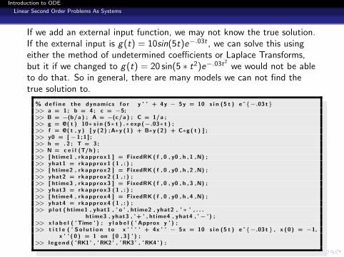
If we add an external input function, we may not know the true solution.If the external input is g(t) = 10sin(5t)e−.03t , we can solve this usingeither the method of undetermined coefficients or Laplace Transforms,but it if we changed to g(t) = 20 sin(5 ∗ t2)e−.03t
2
we would not be ableto do that. So in general, there are many models we can not find thetrue solution to.
% d e f i n e the dynamics f o r y ’ ’ + 4 y − 5 y = 10 s i n (5 t ) eˆ{−.03 t}>> a = 1 ; b = 4 ; c = −5;>> B = −(b/a ) ; A = −(c /a ) ; C = 1/ a ;>> g = @( t ) 10∗ s i n (5∗ t ) .∗ exp (−.03∗ t ) ;>> f = @( t , y ) [ y ( 2 ) ; A∗y ( 1 ) + B∗y ( 2 ) + C∗g ( t ) ] ;>> y0 = [−1 ; 1 ] ;>> h = . 2 ; T = 3 ;>> N = c e i l (T/h ) ;>> [ htime1 , r k a p p r o x 1 ] = FixedRK ( f , 0 , y0 , h , 1 ,N) ;>> yhat1 = r k a p p r o x 1 ( 1 , : ) ;>> [ htime2 , r k a p p r o x 2 ] = FixedRK ( f , 0 , y0 , h , 2 ,N) ;>> yhat2 = r k a p p r o x 2 ( 1 , : ) ;>> [ htime3 , r k a p p r o x 3 ] = FixedRK ( f , 0 , y0 , h , 3 ,N) ;>> yhat3 = r k a p p r o x 3 ( 1 , : ) ;>> [ htime4 , r k a p p r o x 4 ] = FixedRK ( f , 0 , y0 , h , 4 ,N) ;>> yhat4 = r k a p p r o x 4 ( 1 , : ) ;>> p l o t ( htime1 , yhat1 , ’ o ’ , htime2 , yhat2 , ’ ∗ ’ , . . .
ht ime3 , yhat3 , ’ + ’ , htime4 , yhat4 , ’− ’) ;>> x l a b e l ( ’ Time ’ ) ; y l a b e l ( ’ Approx y ’ ) ;>> t i t l e ( ’ S o l u t i o n to x ’ ’ ’ ’ + 4x ’ ’ − 5 x = 10 s i n (5 t ) eˆ{−.03 t } , x ( 0 ) = −1,
x ’ ’ ( 0 ) = 1 on [ 0 , 3 ] ’ ) ;>> l e g e n d ( ’ RK1 ’ , ’ RK2 ’ , ’ RK3 ’ , ’ RK4 ’ ) ;

Introduction to ODE
Linear Second Order Problems As Systems
Note the plot is not quite smooth enough because of the coarsenessof h. Big question is are we getting closer to the true solution?

Introduction to ODE
Linear Second Order Problems As Systems
Homework 70
On all of these problems, for the given stepsize h and final time T ,
generate all four RK order plots as we have done in theexample.
Write this up with attached plots in word.
70.1 For h = .4 and T = 3.
2 u′′(t) + 4 u′(t) − 3 u(t) = exp(−2t) cos(3t)
u(0) = −2
u′(0) = 3
70.2 For h = .2 and T = 4.
u′′(t) − 2 u′(t) + 13 u(t) = 5 exp(−3t) sin(5t)
u(0) = −12
u′(0) = 6
Introduction to ODE
Linear Second Order Problems As Systems
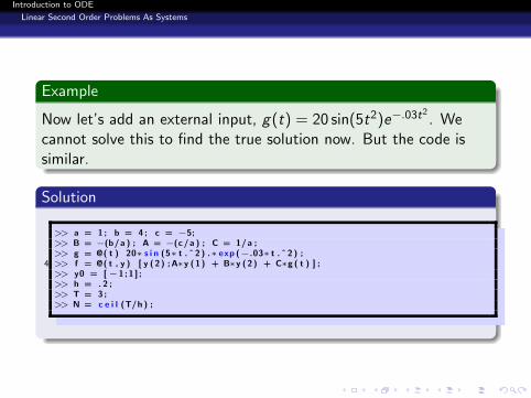
Example
Now let’s add an external input, g(t) = 20 sin(5t2)e−.03t2. We
cannot solve this to find the true solution now. But the code issimilar.
Solution
>> a = 1 ; b = 4 ; c = −5;>> B = −(b/a ) ; A = −(c /a ) ; C = 1/ a ;>> g = @( t ) 20∗ s i n (5∗ t . ˆ 2 ) .∗ exp (−.03∗ t . ˆ 2 ) ;
4 >> f = @( t , y ) [ y ( 2 ) ; A∗y ( 1 ) + B∗y ( 2 ) + C∗g ( t ) ] ;>> y0 = [−1 ; 1 ] ;>> h = . 2 ;>> T = 3 ;>> N = c e i l (T/h ) ;

Introduction to ODE
Linear Second Order Problems As Systems
Solution
>> [ htime1 , r k a p p r o x 1 ] = FixedRK ( f , 0 , y0 , h , 1 ,N) ;2 >> yhat1 = r k a p p r o x 1 ( 1 , : ) ;
>> [ htime2 , r k a p p r o x 2 ] = FixedRK ( f , 0 , y0 , h , 2 ,N) ;>> yhat2 = r k a p p r o x 2 ( 1 , : ) ;>> [ htime3 , r k a p p r o x 3 ] = FixedRK ( f , 0 , y0 , h , 3 ,N) ;>> yhat3 = r k a p p r o x 3 ( 1 , : ) ;
7 >> [ htime4 , r k a p p r o x 4 ] = FixedRK ( f , 0 , y0 , h , 4 ,N) ;>> yhat4 = r k a p p r o x 4 ( 1 , : ) ;>> p l o t ( htime1 , yhat1 , ’o’ , htime2 , yhat2 , ’* ’ , . . .
ht ime3 , yhat3 , ’+ ’ , htime4 , yhat4 , ’-’ ) ;>> x l a b e l ( ’Time ’ ) ;
12 >> y l a b e l ( ’ Approx y’ ) ;>> t i t l e ( ’ Solution to x’’’’ + 4x’’ - 5x =
20 sin (5 t ^2) e ^{ -.03 t^2} , x (0) = -1, x’’(0) = 1 on [0 ,3] ’ ) ;>> l e g e n d ( ’RK1 ’ , ’RK2 ’ , ’RK3 ’ , ’RK4 ’ , ’ Location ’ , ’Best ’ ) ;

Introduction to ODE
Linear Second Order Problems As Systems
This is for h = .2.

Introduction to ODE
Linear Second Order Problems As Systems
Example
Clearly the step size is too large, so let’s decrease it to h = .1 andtry again.
Solution
The code is similar, but there is no true solution now.
>> a = 1 ; b = 4 ; c = −5;>> B = −(b/a ) ; A = −(c /a ) ; C = 1/ a ;>> g = @( t ) 20∗ s i n (5∗ t . ˆ 2 ) .∗ exp (−.03∗ t . ˆ 2 ) ;>> f = @( t , y ) [ y ( 2 ) ; A∗y ( 1 ) + B∗y ( 2 ) + C∗g ( t ) ] ;
5 >> y0 = [−1 ; 1 ] ;>> h = . 1 ;>> T = 3 ;>> N = c e i l (T/h ) ;

Introduction to ODE
Linear Second Order Problems As Systems
Solution
>> [ htime1 , r k a p p r o x 1 ] = FixedRK ( f , 0 , y0 , h , 1 ,N) ;2 >> yhat1 = r k a p p r o x 1 ( 1 , : ) ;
>> [ htime2 , r k a p p r o x 2 ] = FixedRK ( f , 0 , y0 , h , 2 ,N) ;>> yhat2 = r k a p p r o x 2 ( 1 , : ) ;>> [ htime3 , r k a p p r o x 3 ] = FixedRK ( f , 0 , y0 , h , 3 ,N) ;>> yhat3 = r k a p p r o x 3 ( 1 , : ) ;
7 >> [ htime4 , r k a p p r o x 4 ] = FixedRK ( f , 0 , y0 , h , 4 ,N) ;>> yhat4 = r k a p p r o x 4 ( 1 , : ) ;>> p l o t ( htime1 , yhat1 , ’o’ , htime2 , yhat2 , ’* ’ , . . .
ht ime3 , yhat3 , ’+ ’ , htime4 , yhat4 , ’-’ ) ;>> x l a b e l ( ’Time ’ ) ;
12 >> y l a b e l ( ’ Approx y’ ) ;>> t i t l e ( ’ Solution to x’’’’ + 4x’’ - 5x =
20 sin (5 t ^2) e ^{ -.03 t^2} , x (0) = -1, x’’(0) = 1 on [0 ,3] ’ ) ;>> l e g e n d ( ’RK1 ’ , ’RK2 ’ , ’RK3 ’ , ’RK4 ’ , ’ Location ’ , ’Best ’ ) ;

Introduction to ODE
Linear Second Order Problems As Systems
This is for h = .1. Note RK 3 and RK 4 match now.

Introduction to ODE
Linear Second Order Problems As Systems
This is for h = .05. Note RK 3 and RK 4 match now.

Introduction to ODE
Linear Second Order Problems As Systems
This is for h = .01. All RK methods track well for about 1.5 time unitsand then errors get too large. Note h = .01 means 300 iterations. andRK2 is closer.

Introduction to ODE
Linear Second Order Problems As Systems
Homework 71
On all of these problems, for the given stepsize h and final time T ,
generate all four RK order plots as we have done in theexample.
Write this up with attached plots in word.
71.1 For h = .4 and T = 3.
2 u′′(t) + 4 u′(t) − 3 u(t) = exp(−2t2) cos(3t + 5)
u(0) = −2
u′(0) = 3
71.2 For h = .2 and T = 4.
u′′(t) − 2 u′(t) + 13 u(t) = 1 exp(−1.3t) sin(5t2 + 2t + 3)
u(0) = −12
u′(0) = 6

Introduction to ODE
Linear Systems Numerically
We now turn our attention to solving systems of linear ODEsnumerically. We will show you how to do it in two worked outproblems. We then generate the plot of y versus x , the twolines representing the eigenvectors of the problem, the x ′ = 0and the y ′ = 0 lines on the same plot.
A typical MatLab session to solvex ′ = −3x + 4y , y ′ = −x + 2y ; , x(0) = −1; y(0) = 1 wouldlook like this:
f = @( t , x ) [−3∗x ( 1 )+4∗x ( 2 ) ;−x ( 1 )+2∗x ( 2 ) ] ;E1 = @( x ) 0.25∗ x ;E2 = @( x ) x ;xp = @( x ) ( 3 / 4 )∗x ;
5 yp = @( x ) 0.5∗ x ;T = 1 . 4 ;h = . 0 3 ;x0 = [−1 ; 1 ] ;N = c e i l (T/h ) ;

Introduction to ODE
Linear Systems Numerically
We now turn our attention to solving systems of linear ODEsnumerically. We will show you how to do it in two worked outproblems. We then generate the plot of y versus x , the twolines representing the eigenvectors of the problem, the x ′ = 0and the y ′ = 0 lines on the same plot.
A typical MatLab session to solvex ′ = −3x + 4y , y ′ = −x + 2y ; , x(0) = −1; y(0) = 1 wouldlook like this:
1 f = @( t , x ) [−3∗x ( 1 )+4∗x ( 2 ) ;−x ( 1 )+2∗x ( 2 ) ] ;E1 = @( x ) 0.25∗ x ;E2 = @( x ) x ;xp = @( x ) ( 3 / 4 )∗x ;yp = @( x ) 0.5∗ x ;
6 T = 1 . 4 ;h = . 0 3 ;x0 = [−1 ; 1 ] ;N = c e i l (T/h ) ;

Introduction to ODE
Linear Systems Numerically
1 [ ht , r k ] = FixedRK ( f , 0 , x0 , h , 4 ,N) ;X = r k ( 1 , : ) ;Y = r k ( 2 , : ) ;xmin = min (X) ;xmax = max (X) ;
6 xtop = max ( abs ( xmin ) , abs ( xmax ) ) ;ymin = min (Y) ;ymax = max (Y) ;ytop = max ( abs ( ymin ) , abs ( ymax ) ) ;D = max ( xtop , ytop ) ;
11 s = l i n s p a c e (−D, D, 2 0 1 ) ;p l o t ( s , E1 ( s ) , ’-r’ , s , E2 ( s ) , ’-m’ , s , . . .xp ( s ) , ’-b’ , s , yp ( s ) , ’-g’ ,X , Y , ’-k’ ) ;x l a b e l ( ’x’ ) ;y l a b e l ( ’y’ ) ;
16 t i t l e ( ’Phase Plane for Linear System x’’ = -3x+4y,
y’’=-x+2y, x (0) = -1, y (0) = 1’ ) ;l e g e n d ( ’E1 ’ , ’E2 ’ , ’x’’=0 ’ , ’y’’=0 ’ , ’y vs x’ ,’Location ’ , ’Best ’ ) ;

Introduction to ODE
Linear Systems Numerically
This generates this figure.
This matches the qualitative analysis we do by hand, althoughwhen we do it by hand we usually plot a lot of trajectories.

Introduction to ODE
Linear Systems Numerically
Now let’s annotate the code.
1 % Set up the dynamics f o r the modelf = @( t , x ) [−3∗x ( 1 )+4∗x ( 2 ) ;−x ( 1 )+2∗x ( 2 ) ] ;
% E i g e n v e c t o r 1 i s [ 1 ; . 2 5 ] so s l o p e i s . 2 5% s e t up a s t r a i g h t l i n e u s i n g t h i s s l o p eE1 = @( x ) 0.25∗ x ;
6 % E i g e n v e c t o r 2 i s [ 1 ; . 1 ] so s l o p e i s 1% s e t up a s t r a i g h t l i n e u s i n g t h i s s l o p eE2 = @( x ) x ;% the x ’=0 n u l l c l i n e i s −3x+4y = 0 o r y=3/4 x% s e t up a l i n e w i t h t h i s s l o p e
11 xp = @( x ) ( 3 / 4 )∗x ;% the y ’=0 n u l l c l i n e i s −x+2y = 0 o r y = . 5 x% so s e t up a l i n e w i t h t h i s s l o p eyp = @( x ) 0.5∗ x ;
% s e t the f i n a l t ime16 T = 1 . 4 ;
% s e t the s t e p s i z eh = . 0 3 ;% s e t the ICy0 = [−1 ; 1 ] ;
21 % f i n d how many s t e p s we ’ l l t a k eN = c e i l (T/h ) ;

Introduction to ODE
Linear Systems Numerically
% F i n d N a p p r o x i m a t e RK 4 v a l u e s% s t o r e the t i m e s i n ht and the v a l u e s i n r k
3 % r k ( 1 , : ) i s the f i r s t column which i s x% r k ( 2 , : ) i s the second column which i s y[ ht , r k ] = FixedRK ( f , 0 , y0 , h , 4 ,N) ;
% r k ( 1 , : ) i s the f i r s t row which i s s e t to X% r k ( 2 , : ) i s the second row which i s s e t to Y
8 X = r k ( 1 , : ) ;Y = r k ( 2 , : ) ;% the x v a l u e s r a n g e from xmin to xmanxmin = min (X) ;xmax = max (X) ;
13 % f i n d max o f t h e i r a b s o l u t e v a l u e s% example : xmin = −7, xmax = 4 ==> xtop = 7xtop = max ( abs ( xmin ) , abs ( xmax ) ) ;
% the x v a l u e s r a n g e from xmin to xmanymin = min (Y) ;
18 ymax = max (Y) ;% f i n d max o f t h e i r a b s o l u t e v a l u e s% example : ymin = −3, ymax = 10 ==> ytop = 10ytop = max ( abs ( ymin ) , abs ( ymax ) ) ;
% f i n d max o f xtop and ytop ; our example g i v e s D = 1023 D = max ( xtop , ytop ) ;

Introduction to ODE
Linear Systems Numerically
% The p l o t l i v e s i n the box [−D,D] x [−D,D]2 % s e t up a l i n s p a c e o f [−D,D]
s = l i n s p a c e (−D, D, 2 0 1 ) ;% p l o t the e i g e n v e c t o r l i n e s , the n u l l c l i n e s% and Y v s X%−r i s red , −m i s magenta , −b i s b lue ,
7 %−g i s g r e e n and −k i s b l a c kp l o t ( s , E1 ( s ) , ’-r’ , s , E2 ( s ) , ’-m’ , s , xp ( s ) ,’-b’ , s , yp ( s ) , ’-g’ ,X , Y , ’-k’ ) ;
% s e t x and y l a b e l sx l a b e l ( ’x’ ) ;
12 y l a b e l ( ’y’ ) ;% s e t t i t l et i t l e ( ’Phase Plane for Linear System x’’ = -3x+4y,
y’’=-x+2y, x (0) = -1, y (0) = 1’ ) ;% s e t l e g e n d
17 l e g e n d ( ’E1 ’ , ’E2 ’ , ’x’’=0 ’ , ’y’’=0 ’ , ’y vs x’ ,’Location ’ , ’Best ’ ) ;

Introduction to ODE
Linear Systems Numerically
Example
For the system below[x ′(t)y ′(t)
]=
[4 9
−1 −6
] [x(t)y(t)
],
[x(0)y(0)
]=
[4
−2
]
Find the characteristic equation
Find the general solution
Solve the IVP
Solve the System Numerically
Solution
The eigenvalue and eigenvector portion of this solution has alreadybeen done earlier and so we only have to copy the results here.

Introduction to ODE
Linear Systems Numerically
Solution
The characteristic equation is
det
(r
[1 00 1
]−[
4 9−1 −6
])= 0
with eigenvalues r1 = −5 and r2 = 3.
1 For eigenvalue r1 = −5, we found the eigenvector to be[1
−1
].
2 For eigenvalue r2 = 3, we found the eigenvector to be[1
−1/9
]

Introduction to ODE
Linear Systems Numerically
Solution
The general solution to our system is thus[x(t)y(t)
]= A
[1
−1
]e−5t + B
[1
−1/9
]e3t
We solve the IVP by finding the A and B that will give the desiredinitial conditions. This gives[
4−2
]= A
[1
−1
]+ B
[1
−1/9
]or
4 = A + B
−2 = − A +−1
9B

Introduction to ODE
Linear Systems Numerically
Solution
This is easily solved using elimination to give A = 7/4 andB = 9/4. The solution to the IVP is therefore[
x(t)y(t)
]=
7
4
[1
−1
]e−5t +
9
4
[1−19
]e3t
=
[7/4 e−5t + 9/4 e3t
−7/4 e−5t − 1/4 e3t
]We now have all the information needed to solve this numerically.The MatLab session for this problem is given next.

Introduction to ODE
Linear Systems Numerically
Solution
f = @( t , x ) [4∗ x ( 1 )+9∗x ( 2 ) ;−x ( 1 )−6∗x ( 2 ) ] ;2 E1 = @( x ) −1∗x ;
E2 = @( x ) −(1/9)∗x ;xp = @( x ) −(4/9)∗x ;yp = @( x ) −(1/6)∗x ;T = 0 . 4 ;
7 h = . 0 1 ;x0 = [ 4 ;−2 ] ;N = c e i l (T/h ) ;[ ht , r k ] = FixedRK ( f , 0 , x0 , h , 4 ,N) ;X = r k ( 1 , : ) ;
12 Y = r k ( 2 , : ) ;xmin = min (X) ;xmax = max (X) ;xtop = max ( abs ( xmin ) , abs ( xmax ) ) ;ymin = min (Y) ;
17 ymax = max (Y) ;ytop = max ( abs ( ymin ) , abs ( ymax ) ) ;D = max ( xtop , ytop ) ;

Introduction to ODE
Linear Systems Numerically
Solution
1 x = l i n s p a c e (−D, D, 2 0 1 ) ;p l o t ( x , E1 ( x ) , ’-r’ , x , E2 ( x ) , ’-m ’ , x , xp ( x ) ,’-b’ , x , yp ( x ) , ’-c’ ,X , Y , ’-k ’ ) ;x l a b e l ( ’x ’ ) ;y l a b e l ( ’y ’ ) ;
6 t i t l e ( ’Phase Plane for Linear System x’’ = 4x+9y ,
y’’=-x -6y , x (0) = 4, y (0) = -2 ’ ) ;l e g e n d ( ’E1 ’ , ’E2 ’ , ’x’’=0 ’ , ’y ’’=0 ’ ,’y vs x’ , ’ Location ’ , ’Best ’ ) ;
Again this matches the kind of qualitative analysis we have doneby hand, but for only one plot instead of the many trajectories wewould normally sketch. We had to choose the final time T and thestep size h by trial and error to generate the plot you see. If T istoo large, the growth term in the solution generates x and y valuesthat are too big and the trajectory just looks like it lies on top ofthe dominant eigenvector line. The figure we generate is givenbelow.

Introduction to ODE
Linear Systems Numerically

Introduction to ODE
Linear Systems Numerically
Homework 72
For these models,
Find the characteristic equation
Find the general solution
Solve the IVP
Solve the System Numerically
72.1 [x ′(t)y ′(t)
]=
[1 1
−1 −3/2
] [x(t)y(t)
][
x(0)y(0)
]=
[−5−2
]

Introduction to ODE
Linear Systems Numerically
Homework 72
72.2 [x ′(t)y ′(t)
]=
[4 2
−9 −5
] [x(t)y(t)
][
x(0)y(0)
]=
[−1
2
]72.3 [
x ′(t)y ′(t)
]=
[3 74 6
] [x(t)y(t)
][
x(0)y(0)
]=
[−2−3
]

Introduction to ODE
An Attempt At An Automated Phase Plane Plot
Now let’s try to generate a real phase plane portrait by automatingthe phase plane plots for a selection of initial conditions.
1 f u n c t i o n A u t o P h a s e P l a n e P l o t ( fname , s t e p s i z e , . . .t i n i t , t f i n a l , r k o r d e r , . . .x b o x s i z e , y b o x s i z e , . . .
xmin , xmax , ymin , ymax )% fname i s the name o f the model dynamics
6 % s t e p s i z e i s the chosen s t e p s i z e% t i n i t i s the i n i t i a l t ime% t f i n a l i s the f i n a l t ime% r k o r d e r i s the RK o r d e r% we w i l l use i n i t i a l c o n d i t i o n s chosen from the box
11 % [ xmin , xmax ] x [ ymin , ymax ]% T h i s i s done u s i n g the l i n s p a c e command% so x b o x s i z e i s the number o f p o i n t s% i n the i n t e r v a l [ xmin , xmax ]% y b o x s i z e i s the number o f p o i n t s
16 % i n the i n t e r v a l [ ymin , ymax ]% u and v a r e the v e c t o r s we use to compute our I C sn = c e i l ( ( t f i n a l−t i n i t ) / s t e p s i z e ) ;u = l i n s p a c e ( xmin , xmax , x b o x s i z e ) ;v = l i n s p a c e ( ymin , ymax , y b o x s i z e ) ;

Introduction to ODE
An Attempt At An Automated Phase Plane Plot
% h o l d p l o t and c y c l e l i n e c o l o r sx l a b e l ( ’x’ ) ;y l a b e l ( ’y’ ) ;n e w p l o t ;
5 h o l d a l l ;f o r i =1: x b o x s i z e
f o r j =1: y b o x s i z ex0 = [ u ( i ) ; v ( j ) ] ;[ htime , rk , f r k ] = FixedRK ( fname , t i n i t , x0 , . . .
10 s t e p s i z e , r k o r d e r , n ) ;X = r k ( 1 , : ) ;Y = r k ( 2 , : ) ;p l o t (X , Y) ;
end15 end
t i t l e ( ’Phase Plane Plot ’ ) ;h o l d o f f ;
Introduction to ODE
An Attempt At An Automated Phase Plane Plot
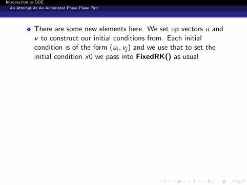
There are some new elements here. We set up vectors u andv to construct our initial conditions from. Each initialcondition is of the form (ui , vj) and we use that to set theinitial condition x0 we pass into FixedRK() as usual
We start by telling MatLab the plot we are going to build is anew one; so the previous plot should be erased. Thecommand hold all then tells MatLab to keep all the plots wegenerate as well as the line colors and so forth until a hold offis encountered.
So here we generate a bunch of plots and we then see themon the same plot at the end! A typical session usually requiresa lot of trial and error. In fact, you should find the analysis byhand is actually more informative!
As discussed, the AutoPhasePlanePlot.m script is used byfilling in values for the inputs it needs. Again the script hasthese inputs:

Introduction to ODE
An Attempt At An Automated Phase Plane Plot
A u t o P h a s e P l a n e P l o t ( fname , s t e p s i z e , t i n i t , t f i n a l , r k o r d e r , . . .x b o x s i z e , y b o x s i z e , xmin , xmax , ymin , ymax )
3 % fname i s the name o f our dynamics f u n c t i o n% s t e p s i z e i s our c a l l , h e r e . 0 1 seems good% t i n i t i s the s t a r t i n g time , h e r e a l w a y s 0% t f i n a l i s hard to p i c k , h e r e% s m a l l seems b e s t ; . 2 − . 6
8 % b e c a u s e one o f our e i g e n v a l u e s i s% p o s i t i v e and the s o l u t i o n% grows too f a s t% r k o r d e r i s the Runge−Kutta o r d e r , h e r e 4% x b o x s i z e i s how many d i f f e r e n t x i n i t i a l v a l u e s
13 % we want , h e r e 4% y b o x s i z e i s how mnay d i f f e r e n t y i n i t i a l v a l u e s% we want , h e r e 4% xmin and xmax g i v e the i n t e r v a l we p i c k% the i n i t i a l x v a l u e s from ;
18 % here , t h e y come from [ − . 3 , . 3 ]% i n the l a s t attempt .% ymin and ymax g i v e the i n t e r v a l we p i c k% the i n i t i a l x v a l u e s from% here , t h e y come from [ − . 3 , . 3 ]
23 % i n the l a s t attempt .

Introduction to ODE
An Attempt At An Automated Phase Plane Plot
Now some attempts for the model[x ′(t)y ′(t)
]=
[4 −18 −5
] [x(t)y(t)
]
We can then try a few phase plane plots.
>> v e c f u n c = @( t , y ) [4∗ y ( 1 )−y ( 2 ) ;8∗ y ( 1 )−5∗y ( 2 ) ] ;>> A u t o P h a s e P l a n e P l o t ( v e c f u n c , . 1 , 0 , 1 , 4 , 4 , 4 ,−1 , 1 ,−1 , 1 ) ;>> A u t o P h a s e P l a n e P l o t ( v e c f u n c , . 0 1 , 0 , . 1 , 4 , 4 , 4 ,−1 , 1 ,−1 , 1 ) ;>> A u t o P h a s e P l a n e P l o t ( v e c f u n c , . 0 1 , 0 , . 4 , 4 , 4 , 4 ,−1 , 1 ,−1 , 1 ) ;>> A u t o P h a s e P l a n e P l o t ( v e c f u n c , . 0 1 , 0 , . 6 , 4 , 4 , 4 ,−1 , 1 ,−1 , 1 ) ;>> A u t o P h a s e P l a n e P l o t ( v e c f u n c , . 0 1 , 0 , . 6 , 4 , 4 , 4 , −1 . 5 , 1 . 5 , −1 . 5 , 1 . 5 ) ;>> A u t o P h a s e P l a n e P l o t ( v e c f u n c , . 0 1 , 0 , . 4 , 4 , 4 , 4 , − . 2 , . 2 , − . 2 , . 2 ) ;>> A u t o P h a s e P l a n e P l o t ( v e c f u n c , . 0 1 , 0 , . 4 , 4 , 4 , 4 , − . 3 , . 3 , − . 3 , . 3 ) ;>> x l a b e l ( ’ x a x i s ’ ) ;>> y l a b e l ( ’ y a x i s ’ ) ;>> t i t l e ( ’ Phase Plane Plot ’ ) ;

Introduction to ODE
An Attempt At An Automated Phase Plane Plot
After a while, we get a plot we like

Introduction to ODE
Further Automation! Eigenvalues in MatLab
We will now discuss certain ways to compute eigenvalues andeigenvectors for a square matrix in MatLab. For a given A, we cancompute its eigenvalues as follows:
>> A = [ 1 2 3 ; 4 5 6 ; 7 8 −1]A =
1 2 34 4 5 6
7 8 −1>> E = e i g (A)E =−0.3954
9 11.8161−6.4206
>>
So we have found the eigenvalues of this small 3 × 3 matrix. Note,in general they are not returned in any sorted order like small tolarge. Bummer!

Introduction to ODE
Further Automation! Eigenvalues in MatLab
To get the eigenvectors, we do this:
>> [ V ,D] = e i g (A)V =
0 . 7 5 3 0 −0.3054 −0.25804 −0.6525 −0.7238 −0.3770
0 . 0 8 4 7 −0.6187 0 . 8 8 9 6D =−0.3954 0 0
0 11.8161 09 0 0 −6.4206
So the eigenvalues here are the diagonal entries in D.

Introduction to ODE
Further Automation! Eigenvalues in MatLab
The eigenvalue/ eigenvector pairs are thus
λ1 = −0.3954, V1 =
0.7530−0.65250.0847
λ2 = 11.8161, V2 =
−0.3054−0.7238−0.6187
λ3 = −6.4206, V3 =
−0.2580−0.37700.8896
MatLab’s eigenvectors are returned having length one. That means take
our usual eigenvector and divide it by its length.

Introduction to ODE
Further Automation! Eigenvalues in MatLab
We have already solves linear models using MatLab tools. Now we willlearn to do a bit more. We begin with a sample problem. Note to analyzea linear systems model, we can do everything by hand, we can then try toemulate the hand work, using computational tools. A sketch of theprocess is thus:
1 For the system below, first do the work by hand.[x ′(t)y ′(t)
]=
[4 −18 −5
] [x(t)y(t)
],
[x(0)y(0)
]=
[−3
1
]Find the characteristic equationFind the general solutionSolve the IVPOn the same x − y graph,
1 draw the x ′ = 0 line, draw the y ′ = 0 line2 draw the eigenvector one line, draw the eigenvector two line3 divide the x − y into four regions corresponding to the
algebraic signs of x ′ and y ′
4 draw the trajectories to create the phase plane portrait
2 Now do the graphical work with MatLab.

Introduction to ODE
Further Automation! Eigenvalues in MatLab
For the problem above, a typical MatLab session would be
1 v e c f u n c = @( t , x ) [4∗ x ( 1 )−x ( 2 ) ;8∗ x ( 1 )−5∗x ( 2 ) ] ;% E1 i s [ 1 ; 8 ] so s l o p e i s 8E1 = @( x ) 8∗x ;% E2 i s [ 1 ; 1 ] so s l o p e i s 1E2 = @( x ) x ;
6 % x ’ = 0 i s 4x−y=0 o r y = 4 xxp = @( x ) 4∗x ;
%y ’=0 i s 8x−5y=0 so 5 y = 8 x o r y = 8/5 xyp = @( x ) ( 8 / 5 )∗x ;T = 0 . 4 ;
11 h = . 0 1 ;x0 = [−3 ; 1 ] ;N = c e i l (T/h ) ;[ ht , rk , f k ] = FixedRK ( v e c f u n c , 0 , x0 , h , 4 ,N) ;X = r k ( 1 , : ) ;
16 Y = r k ( 2 , : ) ;xmin = min (X) ;xmax = max (X) ;xtop = max ( abs ( xmin ) , abs ( xmax ) ) ;ymin = min (Y) ;
21 ymax = max (Y) ;ytop = max ( abs ( ymin ) , abs ( ymax ) ) ;D = max ( xtop , ytop ) ;

Introduction to ODE
Further Automation! Eigenvalues in MatLab
x = l i n s p a c e (−D, D, 2 0 1 ) ;2 p l o t ( x , E1 ( x ) , ’-r’ , x , E2 ( x ) , ’-m’ , x , xp ( x ) , . . .
’-b’ , x , yp ( x ) , ’-c’ ,X , Y , ’-k’ ) ;x l a b e l ( ’x’ ) ;y l a b e l ( ’y’ ) ;t i t l e ( ’Phase Plane for Linear System x’’ = 4x-y,
7 y’’=8x -5y, x (0) = -3, y (0) = 1’ ) ;l e g e n d ( ’E1 ’ , ’E2 ’ , ’x’’=0 ’ , ’y’’=0 ’ , ’y vs x’ ,’Location ’ , ’Best ’ ) ;
This is our old code. We have to find the eigenvalues, eigenvectorsand nullclines by hand and type them into our session. Let’s try todo it better.

Introduction to ODE
Further Automation! Eigenvalues in MatLab
This generates the plot below.

Introduction to ODE
Further Automation! Eigenvalues in MatLab
Consider the new function below:
1 f u n c t i o n Approx = A u t o P h a s e P l a n e P l o t L i n e a r M o d e l ( fname , . . .s t e p s i z e , t i n i t , t f i n a l , r k o r d e r , x b o x s i z e , . . . .y b o x s i z e , xmin , xmax , ymin , ymax , mag)
%% fname i s the name o f the model dynamics
6 % s t e p s i z e i s the chosen s t e p s i z e% t i n i t i s the i n i t i a l t ime% t f i n a l i s the f i n a l t ime% r k o r d e r i s the RK o r d e r% we w i l l use i n i t i a l c o n d i t i o n s chosen from the box
11 % [ xmin , xmax ] x [ ymin , ymax ]% T h i s i s done u s i n g the l i n s p a c e command% so x b o x s i z e i s the number o f p o i n t s% i n the i n t e r v a l [ xmin , xmax ]% and y b o x s i z e i s the number o f p o i n t s
16 % i n the i n t e r v a l [ ymin , ymax ]% mag i s r e l a t e d to the zoom i n l e v e l o f our p l o t .%n = c e i l ( ( t f i n a l−t i n i t ) / s t e p s i z e ) ;

Introduction to ODE
Further Automation! Eigenvalues in MatLab
1 % e x t r a c t a , b , c , and du0 = f e v a l ( fname , 0 , [ 1 ; 0 ] ) ;a = u0 ( 1 ) ;c = u0 ( 2 ) ;v0 = f e v a l ( fname , 0 , [ 0 ; 1 ] ) ;
6 b = v0 ( 1 ) ;d = v0 ( 2 ) ;% now we can c o n s t r u c t AA = [ a , b ; c , d ] ;% g e t e i g e n v a l u e s and e i g e n v e c t o r s
11 [ V ,D] = e i g (A) ;e v a l s = d i a g (D) ;
% the f i r s t column o f V i s E1 , second i s E2E1 = V ( : , 1 ) ;E2 = V ( : , 2 ) ;
16 % The r i s e o v e r run o f E1 i s the s l o p e% The r i s e o v e r run o f E2 i s the s l o p eE 1 s l o p e = E1 ( 2 ) /E1 ( 1 ) ;E 2 s l o p e = E2 ( 2 ) /E2 ( 1 ) ;
% d e f i n e the e i g e n v e c t o r l i n e s21 E 1 l i n e = @( x ) E 1 s l o p e∗x ;
E 2 l i n e = @( x ) E 2 s l o p e∗x ;% s e t u p the n u l l c l i n e l i n e sxp = @( x ) −(a/b )∗x ;yp = @( x ) −(c /d )∗x ;

Introduction to ODE
Further Automation! Eigenvalues in MatLab
% c l e a r out any o l d p i c t u r e sc l fh o l d on
% s e t u p x and y i n i t i a l c o n d i t i o n box5 x i c = l i n s p a c e ( xmin , xmax , x b o x s i z e ) ;
y i c = l i n s p a c e ( ymin , ymax , y b o x s i z e ) ;% f i n d a l l the t r a j e c t o r i e s and s t o r e themApprox = {} ;f o r i =1: x b o x s i z e
10 f o r j =1: y b o x s i z ex0 = [ x i c ( i ) ; y i c ( j ) ] ;[ ht , r k ] = FixedRK ( fname , 0 , x0 , s t e p s i z e , 4 , n ) ;Approx{ i , j } = r k ;U = Approx{ i , j } ;
15 X = U ( 1 , : ) ; Y = U ( 2 , : ) ;% g e t the p l o t t i n g s q u a r e f o r each t r a j e c t o r yumin = min (X) ; umax = max (X) ;utop = max ( abs ( umin ) , abs ( umax ) ) ;vmin = min (Y) ; vmax = max (Y) ;
20 vtop = max ( abs ( vmin ) , abs ( vmax ) ) ;D( i , j ) = max ( utop , vtop ) ;
endend
% g e t the l a r g e s t s q u a r e to put a l l the p l o t s i n t o25 E = max ( max (D) )

Introduction to ODE
Further Automation! Eigenvalues in MatLab
% s e t u p the x l i n s p a c e f o r the p l o tx = l i n s p a c e (−E , E , 2 0 1 ) ;
% s t a r t the h o l dh o l d on
5 % p l o t the e i g e n v e c t o r l i n e s and then the n u l l c l i n e sp l o t ( x , E 1 l i n e ( x ) , ’-r’ , x , E 2 l i n e ( x ) ,’-m’ , x , xp ( x ) , ’-b’ , x , yp ( x ) , ’-c’ ) ;
% l o o p o v e r a l l the ICS and g e t a l l t r a j e c t o r i e sf o r i =1: x b o x s i z e
10 f o r j =1: y b o x s i z eU = Approx{ i , j } ;X = U ( 1 , : ) ; Y = U ( 2 , : ) ;p l o t (X , Y , ’-k’ ) ;
end15 end
% s e t l a b e l s and so f o r t hx l a b e l ( ’x’ ) ; y l a b e l ( ’y’ ) ; t i t l e ( ’Phase Plane ’ ) ;l e g e n d ( ’E1 ’ , ’E2 ’ , ’x’’=0 ’ , ’y’’=0 ’ , ’y vs x’ ,’Location ’ , ’ BestOutside ’ ) ;
20 % s e t zoom f o r p l o t u s i n g maga x i s ([−E∗mag E∗mag −E∗mag E∗mag ] ) ;
% f i n i s h the h o l dh o l d o f f ;end

Introduction to ODE
Further Automation! Eigenvalues in MatLab
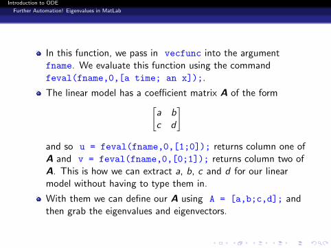
In this function, we pass in vecfunc into the argumentfname. We evaluate this function using the commandfeval(fname,0,[a time; an x]);.
The linear model has a coefficient matrix A of the form[a bc d
]and so u = feval(fname,0,[1;0]); returns column one ofA and v = feval(fname,0,[0;1]); returns column two ofA. This is how we can extract a, b, c and d for our linearmodel without having to type them in.
With them we can define our A using A = [a,b;c,d]; andthen grab the eigenvalues and eigenvectors.

Introduction to ODE
Further Automation! Eigenvalues in MatLab
In this function, we pass in vecfunc into the argumentfname. We evaluate this function using the commandfeval(fname,0,[a time; an x]);.
The linear model has a coefficient matrix A of the form[a bc d
]and so u = feval(fname,0,[1;0]); returns column one ofA and v = feval(fname,0,[0;1]); returns column two ofA. This is how we can extract a, b, c and d for our linearmodel without having to type them in.
With them we can define our A using A = [a,b;c,d]; andthen grab the eigenvalues and eigenvectors.

Introduction to ODE
Further Automation! Eigenvalues in MatLab
Example
In use, for f = @(t,x)[4*x(1)+9*x(2);-x(1)-6*x(2)] we cangenerate nice looking plots and zero in on a nice view with anappropriate use of the parameter max. The E we return is the sizeof the plotting square.
Solution
>> Approx = A u t o P h a s e P l a n e P l o t L i n e a r M o d e l E ( f, . 0 1 , 0 , . 4 5 , 4 , 8 , 8 , − . 5 , . 5 , − . 5 , . 5 , . 2 ) ;
E =4 . 1 4 2 1
>> Approx = A u t o P h a s e P l a n e P l o t L i n e a r M o d e l E ( f, . 0 1 , 0 , . 6 5 , 4 , 8 , 8 , − . 5 , . 5 , − . 5 , . 5 , . 1 ) ;
E =7 . 6 4 8 1

Introduction to ODE
Further Automation! Eigenvalues in MatLab
Solution
>> Approx = A u t o P h a s e P l a n e P l o t L i n e a r M o d e l E ( f, . 0 1 , 0 , . 6 5 , 4 , 1 2 , 1 2 , −1 . 5 , 1 . 5 , −1 . 5 , 1 . 5 , . 1 ) ;
E =22.9443
>> Approx = A u t o P h a s e P l a n e P l o t L i n e a r M o d e l E ( f, . 0 1 , 0 , 1 . 6 5 , 4 , 1 2 , 1 2 , −1 . 5 , 1 . 5 , −1 . 5 , 1 . 5 , . 0 1 ) ;
E =462.3833
>> Approx = A u t o P h a s e P l a n e P l o t L i n e a r M o d e l E ( f, . 0 1 , 0 , 1 . 6 5 , 4 , 1 2 , 1 2 , −1 . 5 , 1 . 5 , −1 . 5 , 1 . 5 , . 0 0 5 ) ;
E =462.3833
>> Approx = A u t o P h a s e P l a n e P l o t L i n e a r M o d e l E ( f, . 0 1 , 0 , 1 . 6 5 , 4 , 6 , 6 , −1 . 5 , 1 . 5 , −1 . 5 , 1 . 5 , . 0 0 5 ) ;
E =462.3833
>> Approx = A u t o P h a s e P l a n e P l o t L i n e a r M o d e l E ( f, . 0 1 , 0 , 1 . 6 5 , 4 , 6 , 6 , −1 . 5 , 1 . 5 , −1 . 5 , 1 . 5 , . 0 0 8 ) ;
E =462.3833

Introduction to ODE
Further Automation! Eigenvalues in MatLab
The last command generates the plot below:

Introduction to ODE
Further Automation! Eigenvalues in MatLab
Homework 73
For a given model
Plot Many Trajectories Simultaneously Using MatLab: This partof the report is done in a word processor withappropriate comments, discussion etc. Show yourMatLab code and sessions as well as plots withappropriate documentation.
Choose Initial Conditions wisely: Choose a useful set of initialconditions to plot trajectories for by choosingxmin, xmax, ymin, ymax, andxboxsize, yboxsize appropriately.
Choose the final time and step size: You’ll also have to find theright final time and step size to use.
Generate a nice phase plane plot: Work hard on generating areally nice phase plane plot by an appropriate use ofthe mag factor.

Introduction to ODE
Further Automation! Eigenvalues in MatLab
Homework 73
73.1 [x ′(t)y ′(t)
]=
[1 1
−1 −3/2
] [x(t)y(t)
]
73.2 [x ′(t)y ′(t)
]=
[4 2
−9 −5
] [x(t)y(t)
]

Introduction to ODE
Further Automation! Eigenvalues in MatLab
Homework 73
73.3 [x ′(t)y ′(t)
]=
[3 74 6
] [x(t)y(t)
]
73.4 [x ′(t)y ′(t)
]=
[1 55 1
] [x(t)y(t)
]