
Solving Dynamic General Equilibrium Models Using Log...
68
... Solving Dynamic General Equilibrium Models Using Log Linear Approximation 1
-
Upload
truongtruc -
Category
Documents
-
view
219 -
download
4
Transcript of Solving Dynamic General Equilibrium Models Using Log...

...
Solving Dynamic General Equilibrium Models UsingLog Linear Approximation
1
Log-linearization strategy
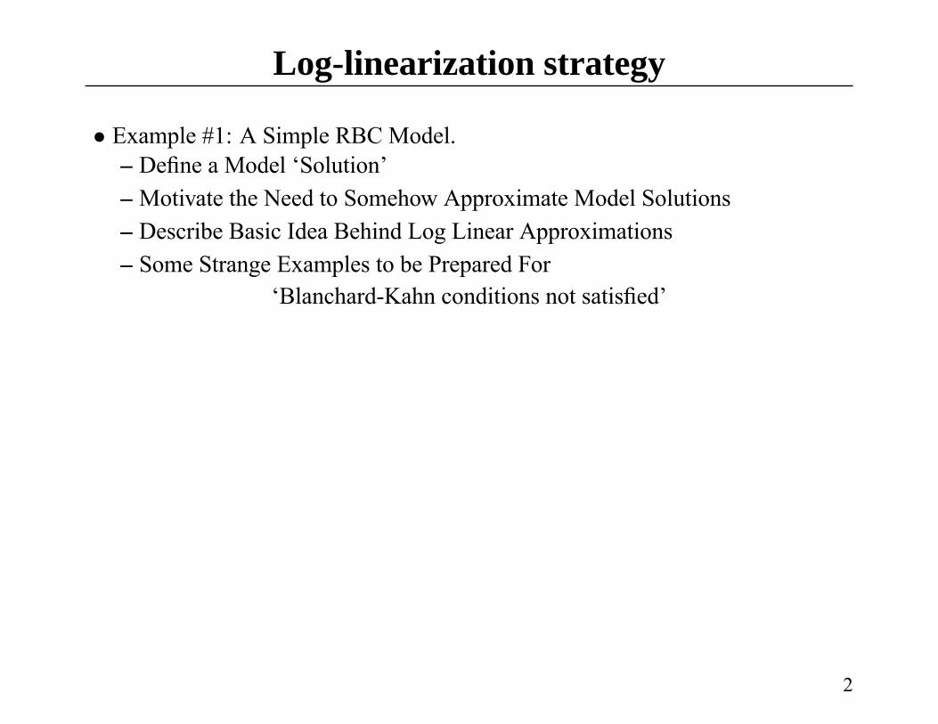
• Example #1: A Simple RBC Model.– Define a Model ‘Solution’– Motivate the Need to Somehow Approximate Model Solutions– Describe Basic Idea Behind Log Linear Approximations– Some Strange Examples to be Prepared For
‘Blanchard-Kahn conditions not satisfied’
2

Log-linearization strategy
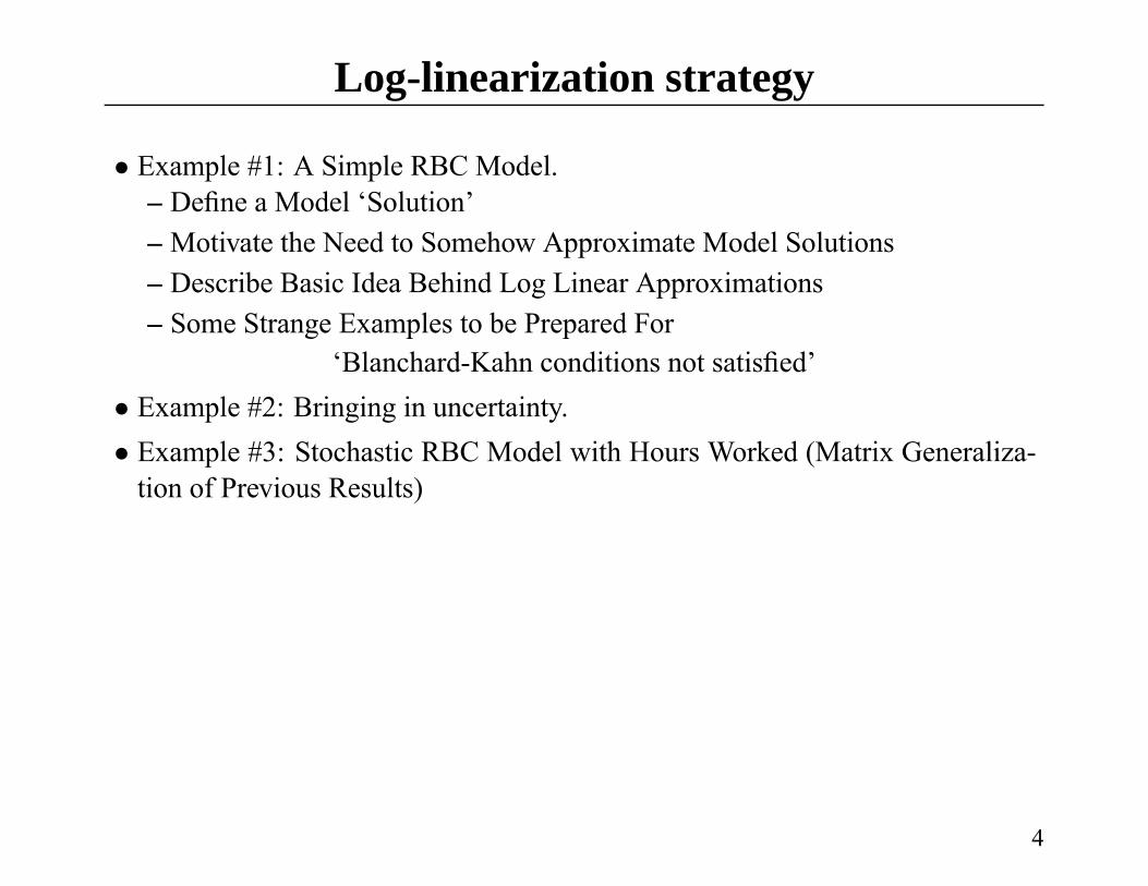
• Example #1: A Simple RBC Model.– Define a Model ‘Solution’– Motivate the Need to Somehow Approximate Model Solutions– Describe Basic Idea Behind Log Linear Approximations– Some Strange Examples to be Prepared For
‘Blanchard-Kahn conditions not satisfied’• Example #2: Bringing in uncertainty.
3
Log-linearization strategy
• Example #1: A Simple RBC Model.– Define a Model ‘Solution’– Motivate the Need to Somehow Approximate Model Solutions– Describe Basic Idea Behind Log Linear Approximations– Some Strange Examples to be Prepared For
‘Blanchard-Kahn conditions not satisfied’• Example #2: Bringing in uncertainty.• Example #3: Stochastic RBC Model with Hours Worked (Matrix Generaliza-
tion of Previous Results)
4

Log-linearization strategy
• Example #1: A Simple RBC Model.– Define a Model ‘Solution’– Motivate the Need to Somehow Approximate Model Solutions– Describe Basic Idea Behind Log Linear Approximations– Some Strange Examples to be Prepared For
‘Blanchard-Kahn conditions not satisfied’• Example #2: Bringing in uncertainty.• Example #3: Stochastic RBC Model with Hours Worked (Matrix Generaliza-
tion of Previous Results)• Example #4: Example #3 with ‘Exotic’ Information Sets.
5
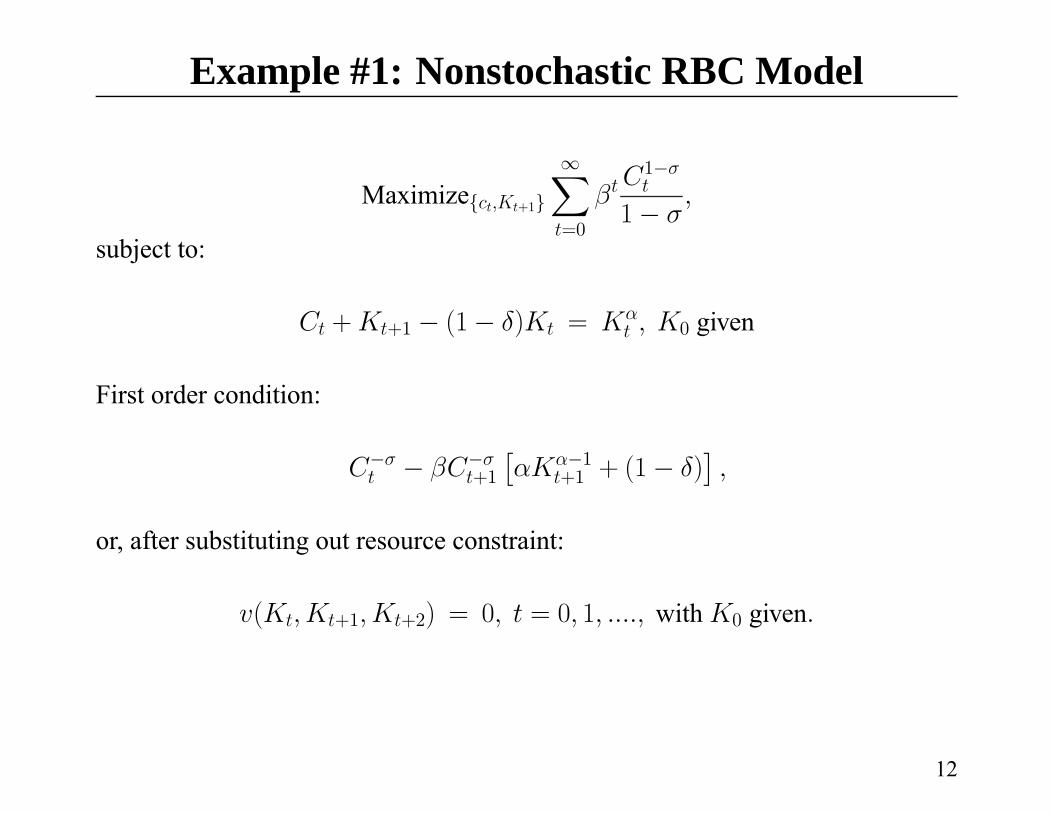
Example #1: Nonstochastic RBC Model
Maximize{ct,Kt+1}
∞Xt=0
βt C1−σt
1− σ,
subject to:
Ct +Kt+1 − (1− δ)Kt = Kαt , K0 given
First order condition:
C−σt − βC−σt+1
£αKα−1
t+1 + (1− δ)¤,
or, after substituting out resource constraint:
v(Kt,Kt+1,Kt+2) = 0, t = 0, 1, ...., with K0 given.
12
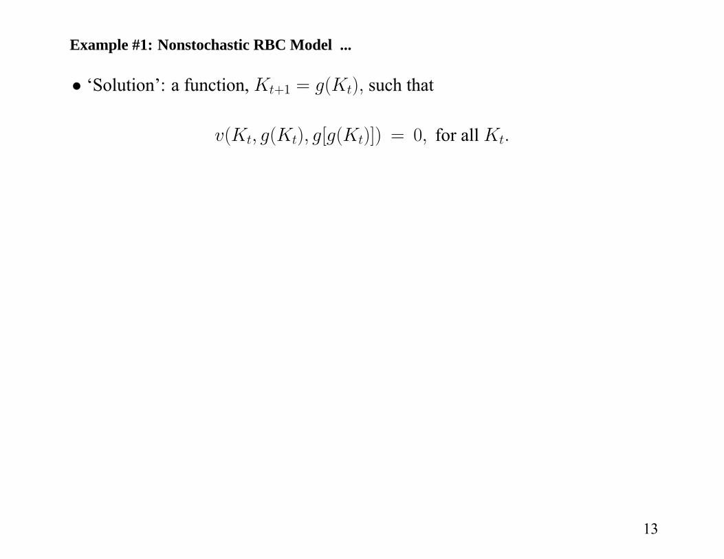
Example #1: Nonstochastic RBC Model ...
• ‘Solution’: a function, Kt+1 = g(Kt), such that
v(Kt, g(Kt), g[g(Kt)]) = 0, for all Kt.
13

Example #1: Nonstochastic RBC Model ...
• ‘Solution’: a function, Kt+1 = g(Kt), such that
v(Kt, g(Kt), g[g(Kt)]) = 0, for all Kt.
• Problem:
This is an Infinite Number of Equations(one for each possible Kt)in an Infinite Number of Unknowns(a value for g for each possible Kt)
14

Example #1: Nonstochastic RBC Model ...
• ‘Solution’: a function, Kt+1 = g(Kt), such that
v(Kt, g(Kt), g[g(Kt)]) = 0, for all Kt.
• Problem:
This is an Infinite Number of Equations(one for each possible Kt)in an Infinite Number of Unknowns(a value for g for each possible Kt)
• With Only a Few Rare Exceptions this is Very Hard to Solve Exactly
15

Example #1: Nonstochastic RBC Model ...
• ‘Solution’: a function, Kt+1 = g(Kt), such that
v(Kt, g(Kt), g[g(Kt)]) = 0, for all Kt.
• Problem:
This is an Infinite Number of Equations(one for each possible Kt)in an Infinite Number of Unknowns(a value for g for each possible Kt)
• With Only a Few Rare Exceptions this is Very Hard to Solve Exactly– Easy cases:∗ If σ = 1, δ = 1⇒ g(Kt) = αβKα
t .∗ If v is linear in Kt, Kt+1, Kt+1.
– Standard Approach: Approximate v by a Log Linear Function.
16
Approximation Method Based on Linearization
• Three Steps– Compute the Steady State– Do a Log Linear Expansion About Steady State– Solve the Resulting Log Linearized System
17

Approximation Method Based on Linearization
• Three Steps– Compute the Steady State– Do a Log Linear Expansion About Steady State– Solve the Resulting Log Linearized System
• Step 1: Compute Steady State -– Steady State Value of K, K∗ -
C−σ − βC−σ£αKα−1 + (1− δ)
¤= 0,
⇒ αKα−1 + (1− δ) =1
β
⇒ K∗ =
"α
1β − (1− δ)
# 11−α
.
– K∗ satisfies:v(K∗, K∗,K∗) = 0.
18

Approximation Method Based on Linearization ...
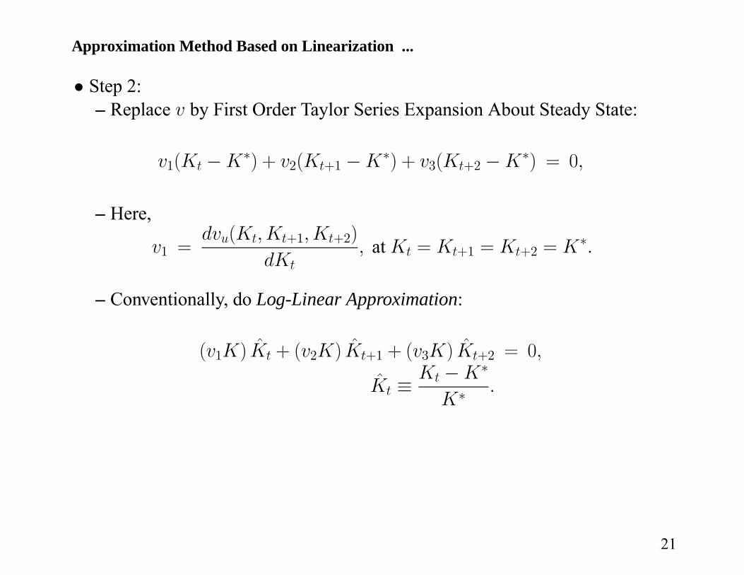
• Step 2:– Replace v by First Order Taylor Series Expansion About Steady State:
v1(Kt −K∗) + v2(Kt+1 −K∗) + v3(Kt+2 −K∗) = 0,
– Here,
v1 =dvu(Kt,Kt+1,Kt+2)
dKt, at Kt = Kt+1 = Kt+2 = K∗.
20
Approximation Method Based on Linearization ...
• Step 2:– Replace v by First Order Taylor Series Expansion About Steady State:
v1(Kt −K∗) + v2(Kt+1 −K∗) + v3(Kt+2 −K∗) = 0,
– Here,
v1 =dvu(Kt,Kt+1,Kt+2)
dKt, at Kt = Kt+1 = Kt+2 = K∗.
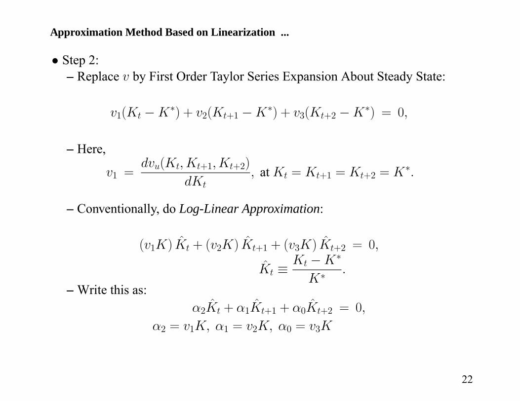
– Conventionally, do Log-Linear Approximation:
(v1K) K̂t + (v2K) K̂t+1 + (v3K) K̂t+2 = 0,
K̂t ≡Kt −K∗
K∗.
21
Approximation Method Based on Linearization ...
• Step 2:– Replace v by First Order Taylor Series Expansion About Steady State:
v1(Kt −K∗) + v2(Kt+1 −K∗) + v3(Kt+2 −K∗) = 0,
– Here,
v1 =dvu(Kt,Kt+1,Kt+2)
dKt, at Kt = Kt+1 = Kt+2 = K∗.
– Conventionally, do Log-Linear Approximation:
(v1K) K̂t + (v2K) K̂t+1 + (v3K) K̂t+2 = 0,
K̂t ≡Kt −K∗
K∗.
– Write this as:α2K̂t + α1K̂t+1 + α0K̂t+2 = 0,
α2 = v1K, α1 = v2K, α0 = v3K
22
Approximation Method Based on Linearization ...
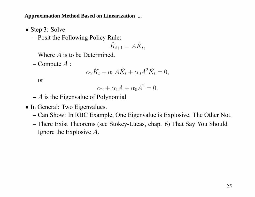
• Step 3: Solve– Posit the Following Policy Rule:
K̂t+1 = AK̂t,
Where A is to be Determined.
23

Approximation Method Based on Linearization ...
• Step 3: Solve– Posit the Following Policy Rule:
K̂t+1 = AK̂t,
Where A is to be Determined.– Compute A :
α2K̂t + α1AK̂t + α0A2K̂t = 0,
orα2 + α1A+ α0A
2 = 0.
– A is the Eigenvalue of Polynomial
24
Approximation Method Based on Linearization ...
• Step 3: Solve– Posit the Following Policy Rule:
K̂t+1 = AK̂t,
Where A is to be Determined.– Compute A :
α2K̂t + α1AK̂t + α0A2K̂t = 0,
orα2 + α1A+ α0A
2 = 0.
– A is the Eigenvalue of Polynomial• In General: Two Eigenvalues.
– Can Show: In RBC Example, One Eigenvalue is Explosive. The Other Not.– There Exist Theorems (see Stokey-Lucas, chap. 6) That Say You Should
Ignore the Explosive A.
25

Some Strange Examples to be Prepared For
• Other Examples Are Possible:– Both Eigenvalues Explosive– Both Eigenvalues Non-Explosive
26
Some Strange Examples to be Prepared For
• Other Examples Are Possible:– Both Eigenvalues Explosive– Both Eigenvalues Non-Explosive– What Do These Things Mean?
27
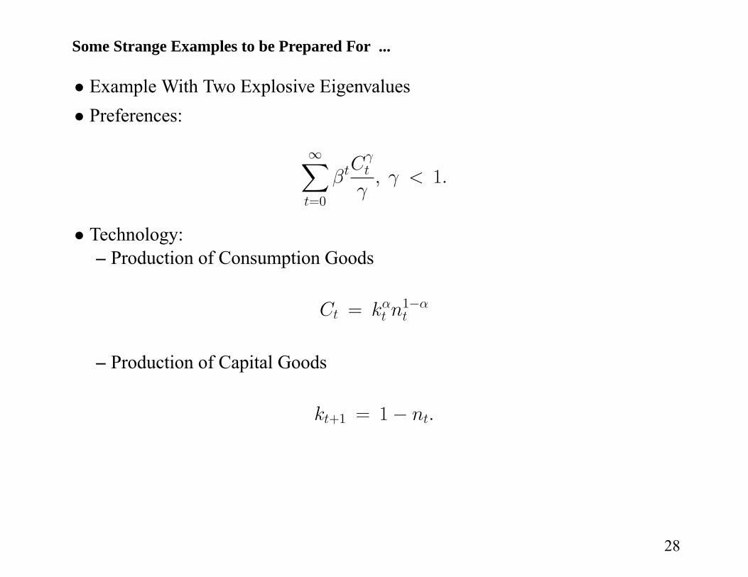
Some Strange Examples to be Prepared For ...
• Example With Two Explosive Eigenvalues• Preferences:
∞Xt=0
βtCγt
γ, γ < 1.
• Technology:– Production of Consumption Goods
Ct = kαt n1−αt
– Production of Capital Goods
kt+1 = 1− nt.
28
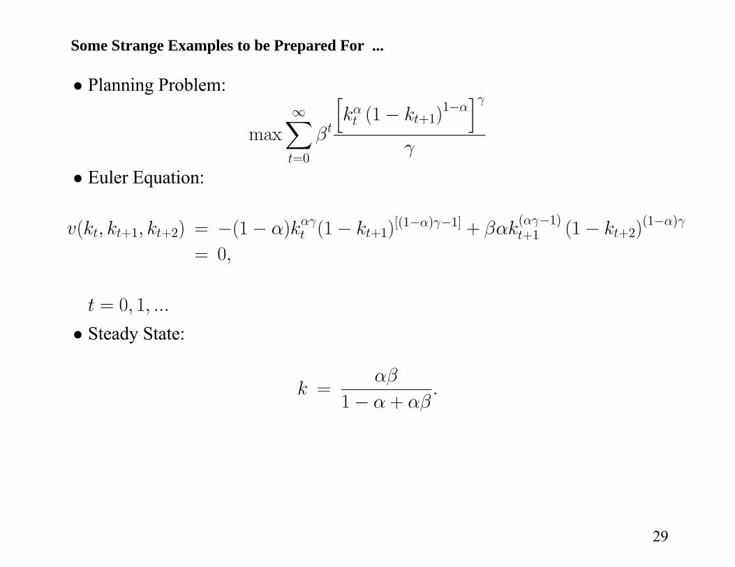
Some Strange Examples to be Prepared For ...
• Planning Problem:
max∞Xt=0
βt
hkαt (1− kt+1)
1−αiγ
γ
• Euler Equation:
v(kt, kt+1, kt+2) = −(1− α)kαγt (1− kt+1)[(1−α)γ−1] + βαk
(αγ−1)t+1 (1− kt+2)
(1−α)γ
= 0,
t = 0, 1, ...
• Steady State:
k =αβ
1− α + αβ.
29
Some Strange Examples to be Prepared For ...
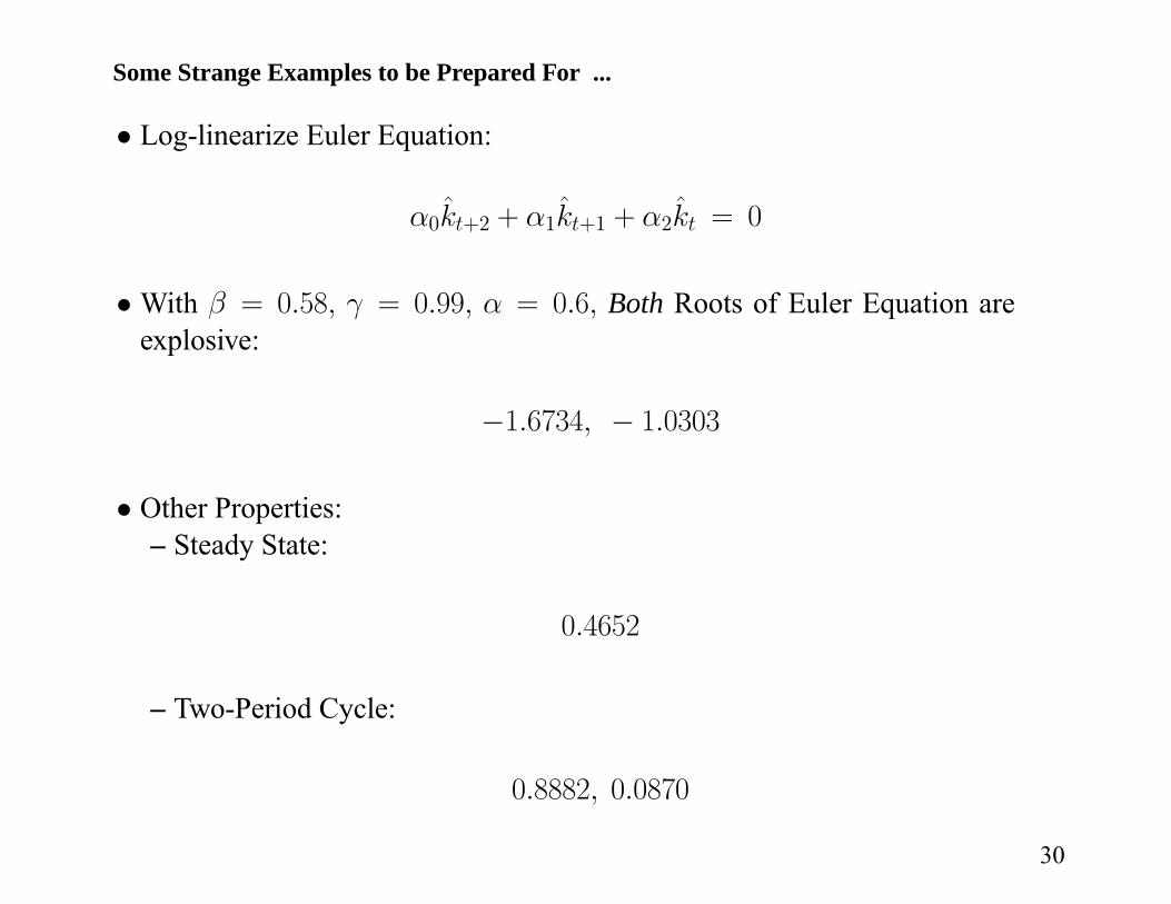
• Log-linearize Euler Equation:
α0k̂t+2 + α1k̂t+1 + α2k̂t = 0
• With β = 0.58, γ = 0.99, α = 0.6, Both Roots of Euler Equation areexplosive:
−1.6734, − 1.0303
• Other Properties:– Steady State:
0.4652
– Two-Period Cycle:
0.8882, 0.0870
30
Some Strange Examples to be Prepared For ...
• Meaning of Stokey-Lucas Example– Illustrates the Possibility of All Explosive Roots
32
Some Strange Examples to be Prepared For ...
• Meaning of Stokey-Lucas Example– Illustrates the Possibility of All Explosive Roots– Economics:∗ If Somehow You Start At Single Steady State, Stay There
33
Some Strange Examples to be Prepared For ...
• Meaning of Stokey-Lucas Example– Illustrates the Possibility of All Explosive Roots– Economics:∗ If Somehow You Start At Single Steady State, Stay There∗ If You are Away from Single Steady State, Go Somewhere Else
34
Some Strange Examples to be Prepared For ...
• Meaning of Stokey-Lucas Example– Illustrates the Possibility of All Explosive Roots– Economics:∗ If Somehow You Start At Single Steady State, Stay There∗ If You are Away from Single Steady State, Go Somewhere Else
– If Log Linearized Euler Equation Around Particular Steady State Has OnlyExplosive Roots∗ All Possible Equilibria Involve Leaving that Steady State∗ Log Linear Approximation Not Useful, Since it Ceases to be Valid
Outside a Neighborhood of Steady State
35
Some Strange Examples to be Prepared For ...
• Meaning of Stokey-Lucas Example– Illustrates the Possibility of All Explosive Roots– Economics:∗ If Somehow You Start At Single Steady State, Stay There∗ If You are Away from Single Steady State, Go Somewhere Else
– If Log Linearized Euler Equation Around Particular Steady State Has OnlyExplosive Roots∗ All Possible Equilibria Involve Leaving that Steady State∗ Log Linear Approximation Not Useful, Since it Ceases to be Valid
Outside a Neighborhood of Steady State– Could Log Linearize About Two-Period Cycle (That’s Another Story...)– The Example Suggests That Maybe All Explosive Root Case is Unlikely
36
Some Strange Examples to be Prepared For ...
• Meaning of Stokey-Lucas Example– Illustrates the Possibility of All Explosive Roots– Economics:∗ If Somehow You Start At Single Steady State, Stay There∗ If You are Away from Single Steady State, Go Somewhere Else
– If Log Linearized Euler Equation Around Particular Steady State Has OnlyExplosive Roots∗ All Possible Equilibria Involve Leaving that Steady State∗ Log Linear Approximation Not Useful, Since it Ceases to be Valid
Outside a Neighborhood of Steady State– Could Log Linearize About Two-Period Cycle (That’s Another Story...)– The Example Suggests That Maybe All Explosive Root Case is Unlikely
– ‘Blanchard-Kahn conditions not satisfied, too many explosive roots’
37

Some Strange Examples to be Prepared For ...
• Another Possibility:
– Both roots stable
– Many paths converge into steady state: multiple equilibria
– How can this happen?∗ strategic complementarities between economic agents.∗ inability of agents to coordinate.∗ combination can lead to multiple equilibria, ‘coordination failures’.
– What is source of strategic complementarities?∗ nature of technology and preferences∗ nature of relationship between agents and the government.
38
Some Strange Examples to be Prepared For ...
• Strategic Complementarities Between Agent A and Agent B– Payoff to agent A is higher if agent B is working harder
39
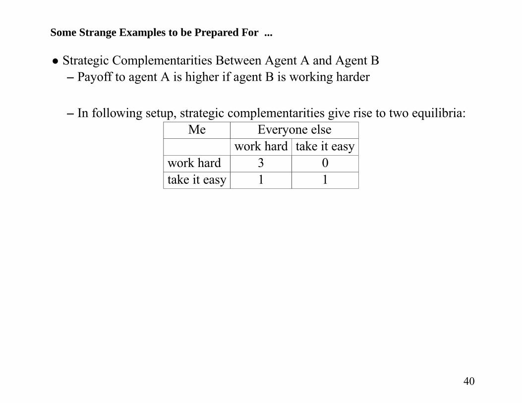
Some Strange Examples to be Prepared For ...
• Strategic Complementarities Between Agent A and Agent B– Payoff to agent A is higher if agent B is working harder
– In following setup, strategic complementarities give rise to two equilibria:Me Everyone else
work hard take it easywork hard 3 0take it easy 1 1
40
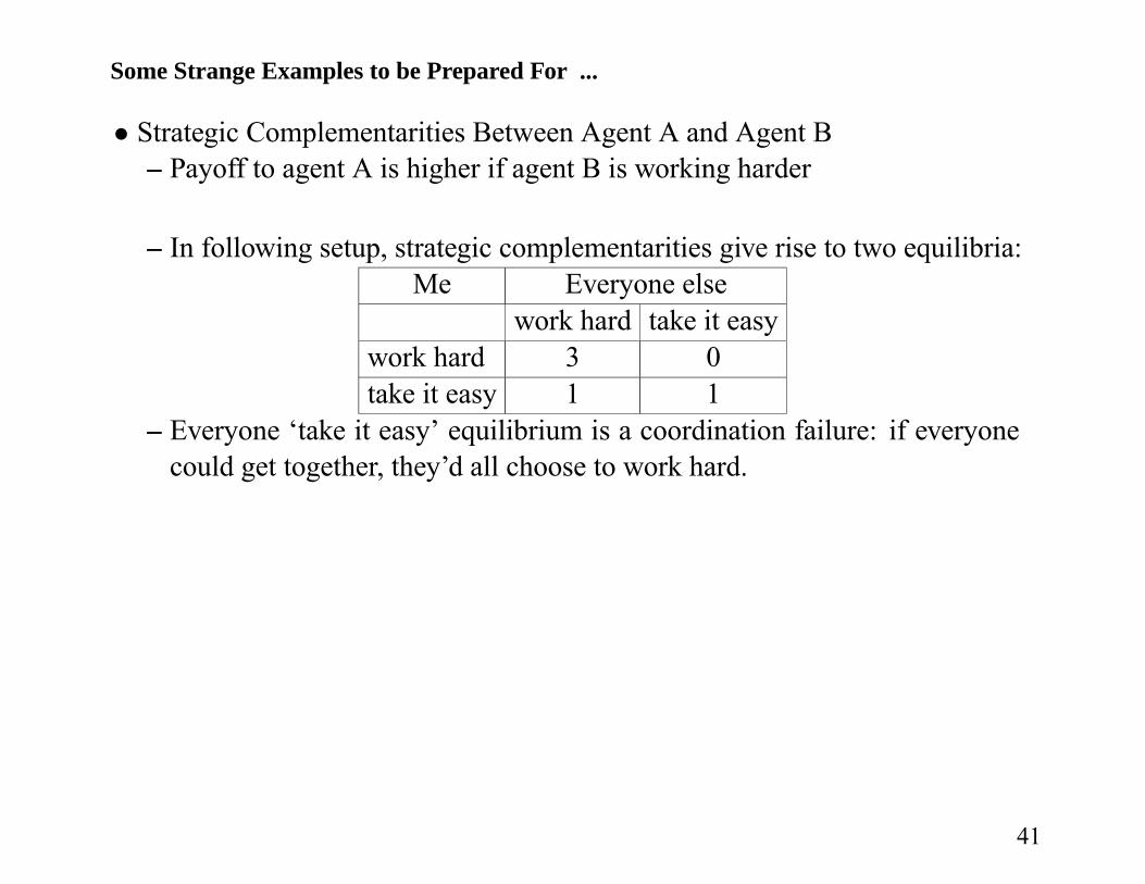
Some Strange Examples to be Prepared For ...
• Strategic Complementarities Between Agent A and Agent B– Payoff to agent A is higher if agent B is working harder
– In following setup, strategic complementarities give rise to two equilibria:Me Everyone else
work hard take it easywork hard 3 0take it easy 1 1
– Everyone ‘take it easy’ equilibrium is a coordination failure: if everyonecould get together, they’d all choose to work hard.
41

Some Strange Examples to be Prepared For ...
• Strategic Complementarities Between Agent A and Agent B– Payoff to agent A is higher if agent B is working harder
– In following setup, strategic complementarities give rise to two equilibria:Me Everyone else
work hard take it easywork hard 3 0take it easy 1 1
– Everyone ‘take it easy’ equilibrium is a coordination failure: if everyonecould get together, they’d all choose to work hard.
– Example closer to home: every firm in the economy has a ‘pet investmentproject’ which only seems profitable if the economy is booming
∗ Equilibrium #1: each firm conjectures all other firms will invest, thisimplies a booming economy, so it makes sense for each firm to invest.∗ Equilibrium #2: each firm conjectures all other firms will not invest, so
economy will stagnate and it makes sense for each firm not to invest.
42

Some Strange Examples to be Prepared For ...
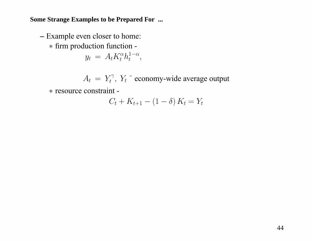
– Example even closer to home:∗ firm production function -
yt = AtKαt h
1−αt ,
At = Y γt , Yt ˜ economy-wide average output
43
Some Strange Examples to be Prepared For ...
– Example even closer to home:∗ firm production function -
yt = AtKαt h
1−αt ,
At = Y γt , Yt ˜ economy-wide average output
∗ resource constraint -Ct +Kt+1 − (1− δ)Kt = Yt
44
Some Strange Examples to be Prepared For ...
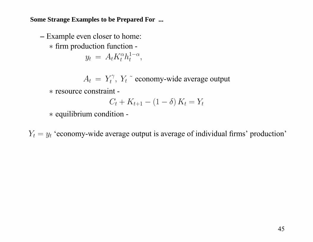
– Example even closer to home:∗ firm production function -
yt = AtKαt h
1−αt ,
At = Y γt , Yt ˜ economy-wide average output
∗ resource constraint -Ct +Kt+1 − (1− δ)Kt = Yt
∗ equilibrium condition -
Yt = yt ‘economy-wide average output is average of individual firms’ production’
45

Some Strange Examples to be Prepared For ...
– Example even closer to home:∗ firm production function -
yt = AtKαt h
1−αt ,
At = Y γt , Yt ˜ economy-wide average output
∗ resource constraint -Ct +Kt+1 − (1− δ)Kt = Yt
∗ equilibrium condition -
Yt = yt ‘economy-wide average output is average of individual firms’ production’
∗ household preferences -∞Xt=0
βtu (Ct, ht)
∗ γ large enough leads to two stable eigenvalues, multiple equilibria.
46

Some Strange Examples to be Prepared For ...
• Lack of commitment in government policy can create strategic complementar-ities that lead to multiple equilibria.
– Simple economy: many atomistic households solve
maxu (c, h) = c− 12l2
c ≤ (1− τ )wh,
w is technologically determined marginal product of labor.
– Government chooses τ to satisfy its budget constraint
g ≤ τwl
47
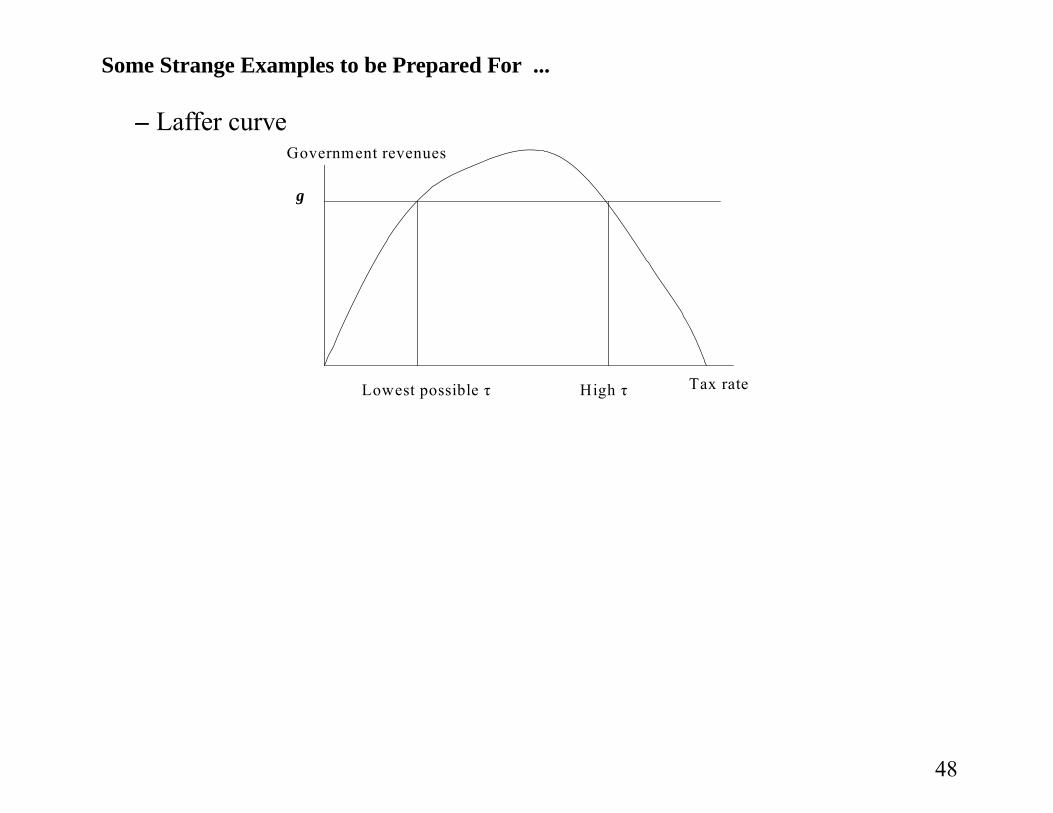
Some Strange Examples to be Prepared For ...
– Laffer curve
g
Government revenues
Tax rate Lowest possible τ High τ
48

Some Strange Examples to be Prepared For ...
– Laffer curve
g
Government revenues
Tax rate Lowest possible τ High τ
– Two scenarios depending on ‘order of moves’∗ commitment: (i) government sets τ (ii) private economy acts· lowest possible τ only possible outcome
∗ no commitment: (i) private economy determines h (ii) government chooses τ· at least two possible equilibria - lowest possible τ or high τ
49

Some Strange Examples to be Prepared For ...
• There is a coordination failure in the Lafffer curve example.....
– If everyone could get together, they would all agree to work hard, so thatthe government sets low taxes ex post.
– But, by assumption, people cannot get together and coordinate.(Also, because individuals have zero impact on government finances, it
makes no sense for an individual person to work harder in the hope that thiswill allow the government to set low taxes.)
• There are strategic complementarities in the previous example
– If I think everyone else will not work hard then, because this will requirethe government to raise taxes, I have an incentive to also not work hard.
• For an environment like this that leads to too many stable eigenvalues, seeSchmitt-Grohe and Uribe paper on balanced budget, JPE.
50

Example #2: RBC Model With Uncertainty
• Model
Maximize E0∞Xt=0
βt C1−σt
1− σ,
subject to
Ct +Kt+1 − (1− δ)Kt = Kαt εt,
where εt is a stochastic process with Eεt = ε, say. Let
ε̂t =εt − ε
ε,
and supposeε̂t = ρε̂t−1 + et, et˜N(0, σ
2e).
• First Order Condition:Et
©C−σt − βC−σt+1
£αKα−1
t+1 εt+1 + 1− 䤪= 0.
51

Example #2: RBC Model With Uncertainty ...
• First Order Condition:Etv(Kt+2,Kt+1,Kt, εt+1, εt) = 0,
wherev(Kt+2,Kt+1,Kt, εt+1, εt)
= (Kαt εt + (1− δ)Kt −Kt+1)
−σ
−β (Kαt+1εt+1 + (1− δ)Kt+1 −Kt+2)
−σ
×£αKα−1
t+1 εt+1 + 1− δ¤.
• Solution: a g(Kt, εt), Such That
Etv (g(g(Kt, εt), εt+1), g(Kt, εt),Kt, εt+1, εt) = 0,
For All Kt, εt.
• Hard to Find g, Except in Special Cases– One Special Case: v is Log Linear.
53
Example #2: RBC Model With Uncertainty ...
• Log Linearization Strategy:
– Step 1: Compute Steady State of Kt when εt is Replaced by Eεt
– Step2: Replace v By its Taylor Series Expansion About Steady State.
– Step 3: Solve Resulting Log Linearized System.
• Logic: If Actual Stochastic System Remains in a Neighborhood of SteadyState, Log Linear Approximation Good
54
Example #2: RBC Model With Uncertainty ...
• Caveat: Strategy not accurate in all conceivable situations.– Example: suppose that where I live -
ε ≡ temperature =½
140 Fahrenheit, 50 percent of time0 degrees Fahrenheit the other half .
– On average, temperature quire nice: Eε = 70 (like parts of California)
– Let K = capital invested in heating and airconditioning
∗ EK very, very large!∗ Economist who predicts investment based on replacing ε by Eε would
predict K = 0 (as in many parts of California)
– In standard model this is not a big problem, because shocks are not sobig....steady state value of K (i.e., the value that results eventually when εis replaced by Eε) is approximately Eε (i.e., the average value of K whenε is stochastic).
55
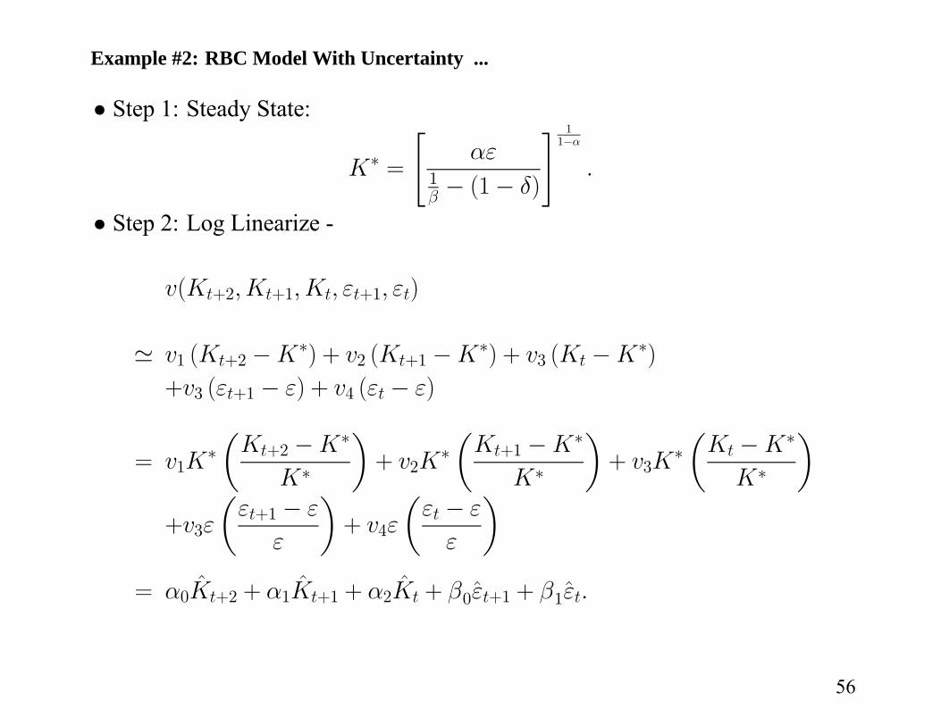
Example #2: RBC Model With Uncertainty ...
• Step 1: Steady State:
K∗ =
"αε
1β − (1− δ)
# 11−α
.
• Step 2: Log Linearize -
v(Kt+2,Kt+1,Kt, εt+1, εt)
' v1 (Kt+2 −K∗) + v2 (Kt+1 −K∗) + v3 (Kt −K∗)
+v3 (εt+1 − ε) + v4 (εt − ε)
= v1K∗µKt+2 −K∗
K∗
¶+ v2K
∗µKt+1 −K∗
K∗
¶+ v3K
∗µKt −K∗
K∗
¶+v3ε
µεt+1 − ε
ε
¶+ v4ε
µεt − ε
ε
¶= α0K̂t+2 + α1K̂t+1 + α2K̂t + β0ε̂t+1 + β1ε̂t.
56

Example #2: RBC Model With Uncertainty ...
• Step 3: Solve Log Linearized System– Posit:
K̂t+1 = AK̂t +Bε̂t.
– Pin Down A and B By Condition that log-linearized Euler Equation MustBe Satisfied.∗ Note:
K̂t+2 = AK̂t+1 +Bε̂t+1= A2K̂t +ABε̂t +Bρε̂t +Bet+1.
∗ Substitute Posited Policy Rule into Log Linearized Euler Equation:
Et
hα0K̂t+2 + α1K̂t+1 + α2K̂t + β0ε̂t+1 + β1ε̂t
i= 0,
so must have:Et{α0
hA2K̂t +ABε̂t +Bρε̂t +Bet+1
i+α1
hAK̂t +Bε̂t
i+ α2K̂t + β0ρε̂t + β0et+1 + β1ε̂t} = 0
57

Example #2: RBC Model With Uncertainty ...
∗ Then,Et
hα0K̂t+2 + α1K̂t+1 + α2K̂t + β0ε̂t+1 + β1ε̂t
i= Et{α0
hA2K̂t +ABε̂t +Bρε̂t +Bet+1
i+α1
hAK̂t +Bε̂t
i+ α2K̂t + β0ρε̂t + β0et+1 + β1ε̂t}
= α(A)K̂t + F ε̂t= 0
whereα(A) = α0A
2 + α1A + α2,
F = α0AB + α0Bρ + α1B + β0ρ + β1
∗ Find A and B that Satisfy:
α(A) = 0, F = 0.
58
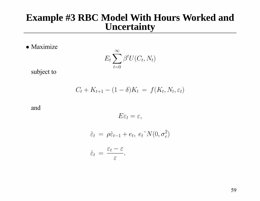
Example #3 RBC Model With Hours Worked andUncertainty
• Maximize
Et
∞Xt=0
βtU(Ct,Nt)
subject to
Ct +Kt+1 − (1− δ)Kt = f(Kt,Nt, εt)
andEεt = ε,
ε̂t = ρε̂t−1 + et, et˜N(0, σ2e)
ε̂t =εt − ε
ε.
59

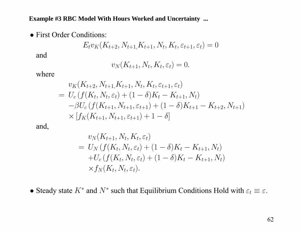
Example #3 RBC Model With Hours Worked and Uncertainty ...
• First Order Conditions:EtvK(Kt+2, Nt+1,Kt+1, Nt,Kt, εt+1, εt) = 0
andvN(Kt+1, Nt,Kt, εt) = 0.
60

Example #3 RBC Model With Hours Worked and Uncertainty ...
• First Order Conditions:EtvK(Kt+2, Nt+1,Kt+1, Nt,Kt, εt+1, εt) = 0
andvN(Kt+1, Nt,Kt, εt) = 0.
wherevK(Kt+2, Nt+1,Kt+1, Nt,Kt, εt+1, εt)
= Uc (f(Kt,Nt, εt) + (1− δ)Kt −Kt+1, Nt)
−βUc (f(Kt+1, Nt+1, εt+1) + (1− δ)Kt+1 −Kt+2, Nt+1)
× [fK(Kt+1, Nt+1, εt+1) + 1− δ]
61
Example #3 RBC Model With Hours Worked and Uncertainty ...
• First Order Conditions:EtvK(Kt+2, Nt+1,Kt+1, Nt,Kt, εt+1, εt) = 0
andvN(Kt+1, Nt,Kt, εt) = 0.
wherevK(Kt+2, Nt+1,Kt+1, Nt,Kt, εt+1, εt)
= Uc (f(Kt,Nt, εt) + (1− δ)Kt −Kt+1, Nt)
−βUc (f(Kt+1, Nt+1, εt+1) + (1− δ)Kt+1 −Kt+2, Nt+1)
× [fK(Kt+1, Nt+1, εt+1) + 1− δ]
and,vN(Kt+1, Nt,Kt, εt)
= UN (f(Kt,Nt, εt) + (1− δ)Kt −Kt+1, Nt)
+Uc (f(Kt,Nt, εt) + (1− δ)Kt −Kt+1, Nt)
×fN(Kt,Nt, εt).
• Steady state K∗ and N∗ such that Equilibrium Conditions Hold with εt ≡ ε.
62
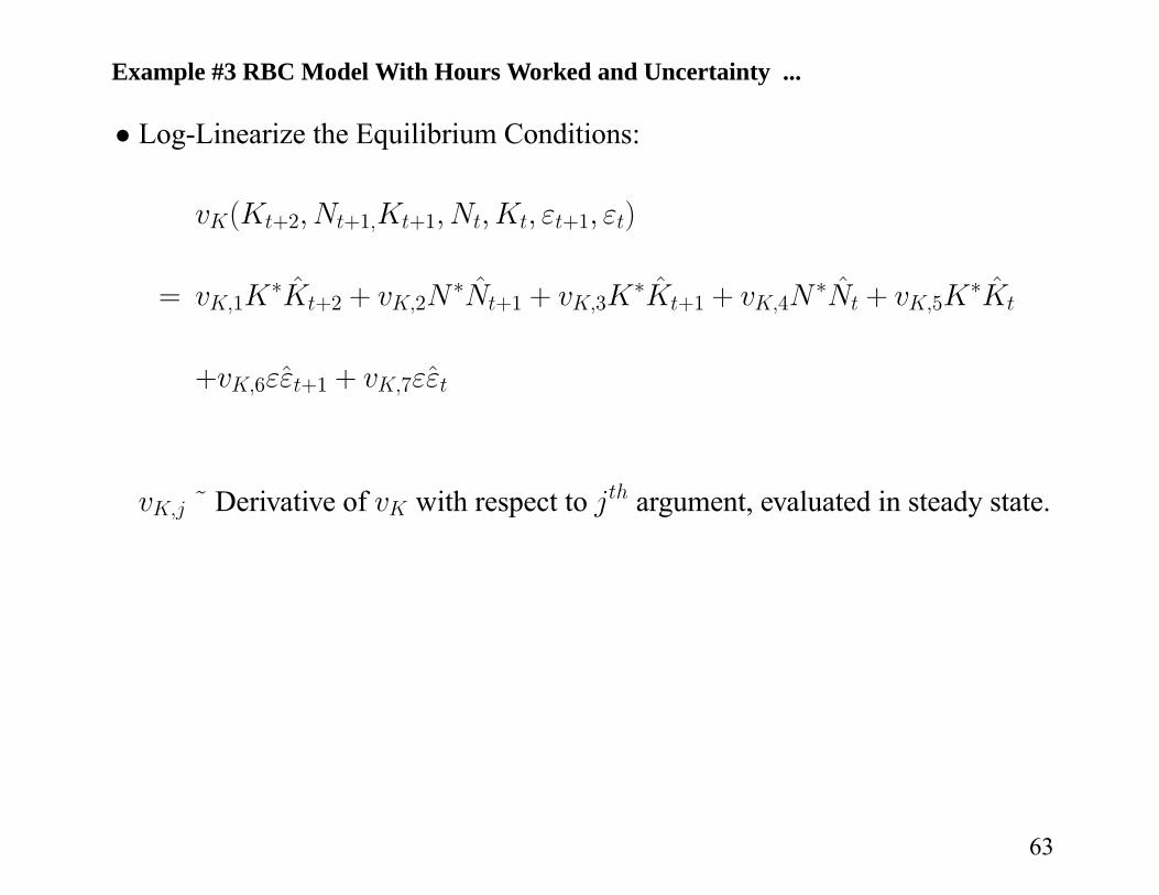
Example #3 RBC Model With Hours Worked and Uncertainty ...
• Log-Linearize the Equilibrium Conditions:
vK(Kt+2, Nt+1,Kt+1, Nt,Kt, εt+1, εt)
= vK,1K∗K̂t+2 + vK,2N
∗N̂t+1 + vK,3K∗K̂t+1 + vK,4N
∗N̂t + vK,5K∗K̂t
+vK,6εε̂t+1 + vK,7εε̂t
vK,j ˜ Derivative of vK with respect to jth argument, evaluated in steady state.
63

Example #3 RBC Model With Hours Worked and Uncertainty ...
• Log-Linearize the Equilibrium Conditions:
vK(Kt+2, Nt+1,Kt+1, Nt,Kt, εt+1, εt)
= vK,1K∗K̂t+2 + vK,2N
∗N̂t+1 + vK,3K∗K̂t+1 + vK,4N
∗N̂t + vK,5K∗K̂t
+vK,6εε̂t+1 + vK,7εε̂t
vK,j ˜ Derivative of vK with respect to jth argument, evaluated in steady state.
vN(Kt+1, Nt,Kt, εt)
= vN,1K∗K̂t+1 + vN,2N
∗N̂t + vN,3K∗K̂t + vN,4εε̂t+1
vN,j ˜ Derivative of vN with respect to jth argument, evaluated in steady state.
64
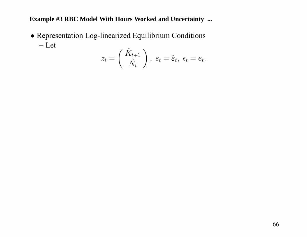
Example #3 RBC Model With Hours Worked and Uncertainty ...
• Representation Log-linearized Equilibrium Conditions– Let
zt =
µK̂t+1
N̂t
¶, st = ε̂t, t = et.
66
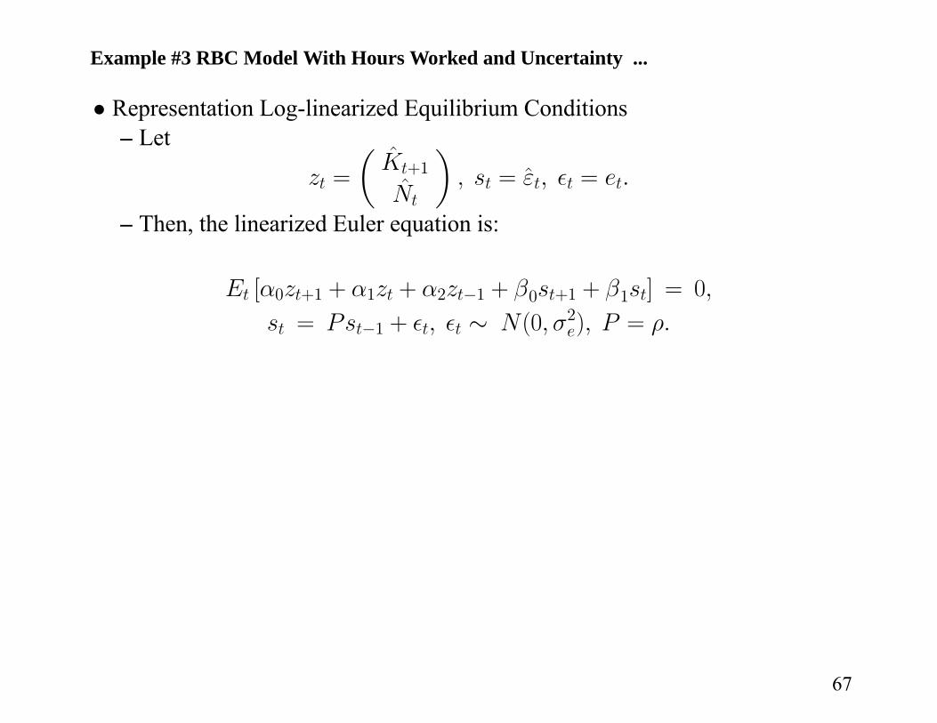
Example #3 RBC Model With Hours Worked and Uncertainty ...
• Representation Log-linearized Equilibrium Conditions– Let
zt =
µK̂t+1
N̂t
¶, st = ε̂t, t = et.
– Then, the linearized Euler equation is:
Et [α0zt+1 + α1zt + α2zt−1 + β0st+1 + β1st] = 0,
st = Pst−1 + t, t ∼ N(0, σ2e), P = ρ.
67
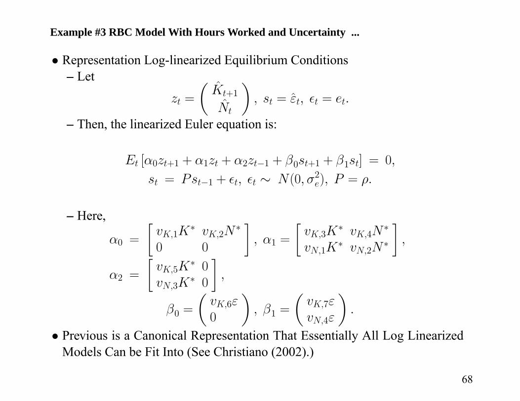
Example #3 RBC Model With Hours Worked and Uncertainty ...
• Representation Log-linearized Equilibrium Conditions– Let
zt =
µK̂t+1
N̂t
¶, st = ε̂t, t = et.
– Then, the linearized Euler equation is:
Et [α0zt+1 + α1zt + α2zt−1 + β0st+1 + β1st] = 0,
st = Pst−1 + t, t ∼ N(0, σ2e), P = ρ.
– Here,
α0 =
∙vK,1K
∗ vK,2N∗
0 0
¸, α1 =
∙vK,3K
∗ vK,4N∗
vN,1K∗ vN,2N
∗
¸,
α2 =
∙vK,5K
∗ 0vN,3K
∗ 0
¸,
β0 =
µvK,6ε0
¶, β1 =
µvK,7εvN,4ε
¶.
• Previous is a Canonical Representation That Essentially All Log LinearizedModels Can be Fit Into (See Christiano (2002).)
68

Example #3 RBC Model With Hours Worked and Uncertainty ...
• Again, Look for Solution
zt = Azt−1 +Bst,
where A and B are pinned down by log-linearized Equilibrium Conditions.• Now, A is Matrix Eigenvalue of Matrix Polynomial:
α(A) = α0A2 + α1A+ α2I = 0.
• Also, B Satisfies Same System of Log Linear Equations as Before:
F = (β0 + α0B)P + [β1 + (α0A+ α1)B] = 0.
• Go for the 2 Free Elements of B Using 2 Equations Given by
F =
∙00
¸.
69

Example #3 RBC Model With Hours Worked and Uncertainty ...
• Finding the Matrix Eigenvalue of the Polynomial Equation,
α(A) = 0,
and Determining if A is Unique is a Solved Problem.• See Anderson, Gary S. and George Moore, 1985, ‘A Linear Algebraic
Procedure for Solving Linear Perfect Foresight Models,’ Economic Letters, 17,247-52 or Articles in Computational Economics, October, 2002. See also, theprogram, DYNARE.
70

Example #3 RBC Model With Hours Worked and Uncertainty ...
• Solving for B– Given A, Solve for B Using Following (Log Linear) System of Equations:
F = (β0 + α0B)P + [β1 + (α0A + α1)B] = 0
71

Example #3 RBC Model With Hours Worked and Uncertainty ...
• Solving for B– Given A, Solve for B Using Following (Log Linear) System of Equations:
F = (β0 + α0B)P + [β1 + (α0A + α1)B] = 0
– To See this, Use
vec(A1A2A3) = (A03 ⊗A1) vec(A2),
72

Example #3 RBC Model With Hours Worked and Uncertainty ...
• Solving for B– Given A, Solve for B Using Following (Log Linear) System of Equations:
F = (β0 + α0B)P + [β1 + (α0A + α1)B] = 0
– To See this, Use
vec(A1A2A3) = (A03 ⊗A1) vec(A2),
to Convert F = 0 Into
vec(F 0) = d + qδ = 0, δ = vec(B0).
– Find B By First Solving:
δ = −q−1d.
73

Example #4: Example #3 With ‘Exotic’Information Set
• Suppose the Date t Investment Decision is Made Before the Current Realiza-tion of the Technology Shock, While the Hours Decision is Made Afterward.
• Now, Canonical Form Must Be Written Differently:
Et [α0zt+1 + α1zt + α2zt−1 + β0st+1 + β1st] = 0,
whereEtXt =
∙E [X1t|ε̂t−1]E [X2t|ε̂t]
¸.
• Convenient to Change st:
st =
µε̂tε̂t−1
¶, P =
∙ρ 01 0
¸, t =
µet0
¶.
• Adjust βi’s:
β0 =
µvK,6ε 00 0
¶, β1 =
µvK,7ε 0vN,4ε 0
¶,
74
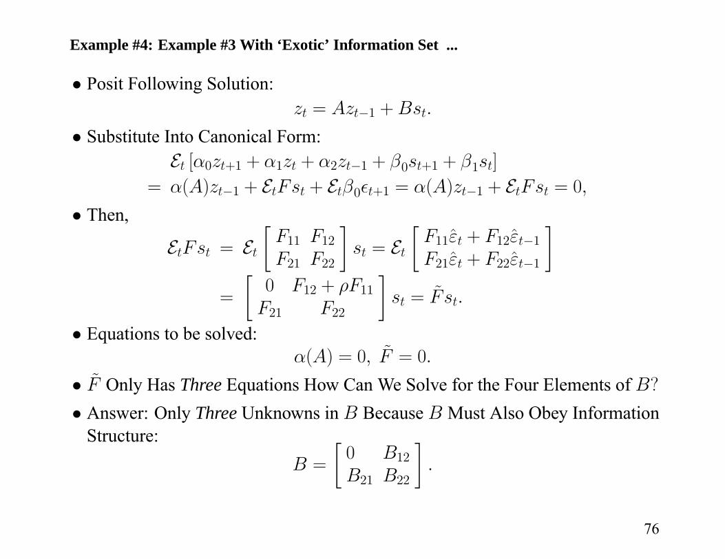
Example #4: Example #3 With ‘Exotic’ Information Set ...
• Posit Following Solution:zt = Azt−1 +Bst.
• Substitute Into Canonical Form:Et [α0zt+1 + α1zt + α2zt−1 + β0st+1 + β1st]
= α(A)zt−1 + EtFst + Etβ0 t+1 = α(A)zt−1 + EtFst = 0,• Then,
EtFst = Et∙F11 F12F21 F22
¸st = Et
∙F11ε̂t + F12ε̂t−1F21ε̂t + F22ε̂t−1
¸=
∙0 F12 + ρF11F21 F22
¸st = F̃ st.
• Equations to be solved:α(A) = 0, F̃ = 0.
• F̃ Only Has Three Equations How Can We Solve for the Four Elements of B?• Answer: Only Three Unknowns in B Because B Must Also Obey Information
Structure:B =
∙0 B12B21 B22
¸.
76
Summary so Far
• Solving Models By Log Linear Approximation Involves Three Steps:a. Compute Steady Stateb. Log-Linearize Equilibrium Conditionsc. Solve Log Linearized Equations.
77
Summary so Far
• Solving Models By Log Linear Approximation Involves Three Steps:a. Compute Steady Stateb. Log-Linearize Equilibrium Conditionsc. Solve Log Linearized Equations.
• Step 3 Requires Finding A and B in:zt = Azt−1 +Bst,
to Satisfy Log-Linearized Equilibrium Conditions:Et [α0zt+1 + α1zt + α2zt−1 + β0st+1 + β1st]
st = Pst−1 + t, t ∼ iid
78

Summary so Far
• Solving Models By Log Linear Approximation Involves Three Steps:a. Compute Steady Stateb. Log-Linearize Equilibrium Conditionsc. Solve Log Linearized Equations.
• Step 3 Requires Finding A and B in:zt = Azt−1 +Bst,
to Satisfy Log-Linearized Equilibrium Conditions:Et [α0zt+1 + α1zt + α2zt−1 + β0st+1 + β1st]
st = Pst−1 + t, t ∼ iid• We are Led to Choose A and B so that:
α(A) = 0,
(standard information set) F = 0,
(exotic information set) F̃ = 0
and Eigenvalues of A are Less Than Unity In Absolute Value.
79