Understanding the Effects of a Shock to Government...
41
Ž . Review of Economic Dynamics 2, 166]206 1999 Article ID redy.1998.0036, available online at http:rrwww.idealibrary.com on Understanding the Effects of a Shock to Government Purchases* Wendy Edelberg Department of Economics, Uni ¤ ersity of Chicago, Chicago, Illinois 60637 Martin Eichenbaum Department of Economics, Northwestern Uni ¤ ersity, E¤ anston, Illinois 60208 and Jonas D. M. Fisher Economic Research Department, Federal Reser ¤ e Bank of Chicago, Chicago, Illinois 60604-1413 E-mail: [email protected] Received December 1997 This paper investigates the consequences of an exogenous increase in U.S. government purchases. We find that in response to such a shock, employment, output, and nonresidential investment rise, while real wages, residential invest- ment, and consumption expenditures fall. The paper argues that a simple variant of the neoclassical growth model which distinguishes between nonresidential and residential investment is consistent with this evidence. Journal of Economic Litera- ture Classification Numbers: E1, E6. Q 1999 Academic Press 1. INTRODUCTION This paper investigates the consequences of an exogenous increase in U.S. government purchases. Consistent with results of Ramey and Shapiro Ž . 1997 we find that, in response to such a shock, employment, output, and nonresidential investment rise, while real wages, residential investment, * The views expressed in this paper do not necessarily represent the views of the Federal Reserve Bank of Chicago or the Federal Reserve System. Martin Eichenbaum gratefully acknowledges the financial support of a grant from the National Science Foundation to the National Bureau of Economic Research. 166 1094-2025r99 $30.00 Copyright Q 1999 by Academic Press All rights of reproduction in any form reserved.
Transcript of Understanding the Effects of a Shock to Government...

Ž .Review of Economic Dynamics 2, 166]206 1999Article ID redy.1998.0036, available online at http:rrwww.idealibrary.com on
Understanding the Effects of a Shock to GovernmentPurchases*
Wendy Edelberg
Department of Economics, Uni ersity of Chicago, Chicago, Illinois 60637
Martin Eichenbaum
Department of Economics, Northwestern Uni ersity, E¨anston, Illinois 60208
and
Jonas D. M. Fisher
Economic Research Department, Federal Reser e Bank of Chicago, Chicago, Illinois60604-1413
E-mail: [email protected]
Received December 1997
This paper investigates the consequences of an exogenous increase in U.S.government purchases. We find that in response to such a shock, employment,output, and nonresidential investment rise, while real wages, residential invest-ment, and consumption expenditures fall. The paper argues that a simple variant ofthe neoclassical growth model which distinguishes between nonresidential andresidential investment is consistent with this evidence. Journal of Economic Litera-ture Classification Numbers: E1, E6. Q 1999 Academic Press
1. INTRODUCTION
This paper investigates the consequences of an exogenous increase inU.S. government purchases. Consistent with results of Ramey and ShapiroŽ .1997 we find that, in response to such a shock, employment, output, andnonresidential investment rise, while real wages, residential investment,
* The views expressed in this paper do not necessarily represent the views of the FederalReserve Bank of Chicago or the Federal Reserve System. Martin Eichenbaum gratefullyacknowledges the financial support of a grant from the National Science Foundation to theNational Bureau of Economic Research.
1661094-2025r99 $30.00Copyright Q 1999 by Academic PressAll rights of reproduction in any form reserved.

SHOCK TO GOVERNMENT PURCHASES 167
and consumption expenditures fall. We argue that a simple variant of theneoclassical growth model which distinguishes between nonresidential andresidential investment is consistent with this evidence.
There are various reasons to be interested in what happens to theeconomy after an exogenous increase in government purchases. We focuson this question because the answer to it is useful as part of a particularlimited information strategy for assessing the empirical plausibility ofcompeting business cycle models. The essence of this strategy is to com-pare the predictions of different models for how the economy responds toa particular shock.1
To be a useful part of such a diagnostic strategy, a shock must satisfythree criteria. First, different models must react differently to the shock.Second, we must understand the nature of the experiment involved. Forexample, does the candidate shock lead to transitory or persistent changesin the variable that has been shocked? Third, we must know how theactual economy responds to such a shock.
Shocks to government purchases clearly satisfy the first criterion.2 It iswell known that different models react differently to exogenous changes ingovernment purchases.3 In the neoclassical models analyzed by Aiyagari
Ž . Ž . Ž .et al. 1992 , Christiano and Eichenbaum 1992 , Baxter and King 1993 ,Ž .and Burnside and Eichenbaum 1996 , an exogenous increase in govern-
ment purchases, financed by lump-sum taxes, raises output and the realinterest rate but reduces consumption and real wages.4 In the multisector
Ž . Ž .models of Phelan and Trejos 1996 and Ramey and Shapiro 1997 , anexogenous increase in government purchases can lead to either a rise or afall in real wages, depending on how they are measured. In addition,sectoral output may rise or fall, depending on the sector in question.
Ž .Rotemberg and Woodford 1992 study the effects of changes in govern-ment purchases in a model which incorporates increasing returns andoligopolistic pricing. In sharp contrast to the one-sector models above,their model implies that a positive shock to government purchases raises
Ž .real wages. Similarly, in the model of Devereux et al. 1996 , which alsoassumes the presence of increasing returns and imperfect competition, anexogenous increase in government purchases raises private consumptionand real wages.
While shocks to government purchases satisfy the first criterion, it is lessclear that they satisfy the second and third criteria. As Ramey and Shapiro
1 Ž .See Christiano et al. 1997 as well as the references therein for a discussion of thisstrategy as applied to exogenous monetary policy shocks.
2 Here and throughout the paper, the term ‘‘government purchases refers to government3 Ž .See Ramey and Shapiro 1997 for a useful summary of the literature.4 Ž .Aiyagari et al. 1992 point out that the sign of the response of the interest rate depends
on the utility function of the representative consumer.

EDELBERG, EICHENBAUM, AND FISHER168
Ž .1997 stress, there has been relatively little work done on identifying theeffects exogenous shocks to government purchases on the economy. Three
Ž .important exceptions are the studies by Blanchard and Perotti 1998 ,Ž . Ž .Rotemberg and Woodford 1992 , and Ramey and Shapiro 1997 . Blan-
Ž .chard and Perotti 1998 use institutional information about the tax andtransfer systems in different countries to construct an exactly identified
Ž .Vector Autoregression VAR for real output, taxes, and governmentpurchases. This allows them to identify the effects of fiscal shocks on totaloutput. While certainly of interest, their study does not directly help todiscriminate between the competing models discussed above. This is be-cause all of those models predict that real output should rise after anexogenous increase in government purchases. Rotemberg and WoodfordŽ .1992 identify exogenous movements in government purchases with statis-tical innovations to defense purchases in a VAR that contains a small list
Ž .of variables. In contrast, Ramey and Shapiro 1997 use the ‘‘narrativeapproach’’ to isolate political events that led to three large militarybuildups which were arguably unrelated to developments in the domesticU.S. economy. Throughout this paper we refer to their estimates of thedates at which these events began as the Ramey]Shapiro episodes. Thebasic strategy underlying the empirical analysis of Ramey and Shapiro is toexamine the behavior of the U.S. economy after the onset of theseepisodes.
In our view there are at least three reasons for being skeptical ofVAR-based innovations to real defense purchase as measures of exoge-nous shocks to government purchases. First, the estimated innovations mayreflect shocks to the private sector that cause defense contractors tooptimally rearrange delivery schedules, say because of strikes or otherdevelopments in the private sector. Indeed according to Ramey and
Ž .Shapiro 1997, p. 40 ; ‘‘many of the disturbances in the VAR approach aredue solely to timing effects on military contracts and do not representunanticipated changes in military spending.’’ Second, private agents andthe government may know about a planned increase in defense purchaseswell before it is recorded in the data. For example, suppose that at time tthe fiscal authority receives information that causes it to commit to astream of defense purchases in the future, say because North Koreaattacks South Korea. The space spanned by the variables in a small VARmay not contain this information. Under these circumstances an econome-trician will uncover, at best, a polluted measure of exogenous shocks togovernment purchases. Finally, inference from innovation-based measuresof shocks to government purchases appears to be quite fragile to perturba-tions in the sample period used, as well as the list of variables included in
Ž .the VAR see Christiano, 1990 .

SHOCK TO GOVERNMENT PURCHASES 169
For these reasons, we adopt an extended version of the Ramey]Shapiroapproach in our empirical work. Our main findings are that in response toan expansionary shock in government purchases,
v defense expenditures as well as total government purchases rise;
v output rises, both in the aggregate and in all sectors that we look at;
v real wages fall;
v nonresidential investment rises sharply;
v residential investment declines sharply;
v after a delay, purchases and production of consumer durables andnondurables fall;
v real interest rates initially fall but then rise.
A novel feature of our analysis is that we attempt to confront uncer-tainty about the actual dates at which the Ramey]Shapiro episodes began.That there is uncertainty about the dates is evident once we recognize thatthe key issue is when U.S. economic agents understood that a militarybuildup was going to begin. It is one thing to know when the NorthKoreans attacked South Korea. However, ascertaining when economicagents know that the United States was going to respond is a far moresubtile empirical issue. To deal with this issue, we provide evidence thatour results are robust to date uncertainty. At the same time we alsodocument that the Ramey]Shapiro dates are unusual, relative to other,arbitrarily selected dates in the sample. These finding support the inter-pretation that we have isolated the response of the U.S. economy toexogenous increases in government purchases per se.
Taking this interpretation as given, we develop a modified version of theone-sector neoclassical growth model to interpret our estimated responsefunctions. Our modifications are motivated by the following issues. First, inthe standard one-sector growth model, a highly persistent shock to govern-ment purchases leads to a large fall in consumption. In the data, however,these is only a small fall in purchases of consumer nondurable goods andservices after a Ramey]Shapiro episode. Second, the standard one-sectormodel is silent on the question of why residential investment falls whilenonresidential investment rises after a positive shock to government pur-chases.
To understand our strategy for addressing these issues, recall that in thestandard neoclassical growth model, a persistent rise in government pur-chases raises the present value of the representative household’s tax
IBM USER
Highlight

EDELBERG, EICHENBAUM, AND FISHER170
burden. The resulting negative wealth effect increases household’s laborsupply and lowers the demand for private consumption. As a consequence,equilibrium real wages and private consumption fall while employmentincreases. With capital and labor being complements in production, invest-ment rises.5
With this in mind, we modify the basic model to distinguish between twotypes of capital. The first type is used to produce goods. Investment innonresidential capital augments this type of capital. Like any durableconsumption good, the second type of capital yields consumption services.Investment in residential structures, i.e., housing, augments this type of
Žcapital for the sake of simplicity, we do not distinguish between durable.consumption goods and housing . With this modification, the negative
income effect associated with a persistent increase in government pur-chases leads to a rise in nonresidential investment, and a substantial fall inconsumption service flows. The latter is achieved, in part, by lowering thestock of residential capital and a fall in residential investment. As in thestandard model, total output rises and real wages fall. We conclude thatour model can account for the basic qualitati e response of the U.S.economy to a persistent shock in government purchases.
While our empirical results are consistent with this simple variant of theneoclassical model, they pose a sharp challenge to models like that of
Ž . Ž .Rotemberg and Woodford 1992 and Devereux et al. 1996 , in which realwages rise after a positive shock to government purchases. One of the keyempirical results in our paper is that real wages fall after such a shock.This is true regardless of whether we analyze aggregate or sector specificreal wages. It is also true regardless of whether we consider before- orafter-tax real wages. Finally, this result is robust across the different priceindices that we use to construct alternative measures of the real wage.Based on this evidence we conclude that models in which real wages riseafter a positive shock to government purchases are inconsistent with thedata.
The remainder of this paper is organized as follows. In Section 2 wediscuss our methodology for identifying the effects of an exogenous in-crease in government purchases. Section 3 reports the results of imple-menting this methodology on post]World War II U.S. data. Section 4presents our model and assesses its ability to account for the empiricalfindings of Section 3. Finally, Section 5 discusses some shortcomings of ourmodel.
5 If the rise of government purchases induced by the shock is transitory, employment willrise while investment falls. See Section 4.
SHOCK TO GOVERNMENT PURCHASES 171
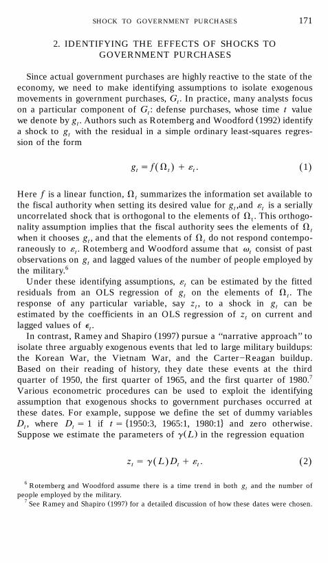
2. IDENTIFYING THE EFFECTS OF SHOCKS TOGOVERNMENT PURCHASES
Since actual government purchases are highly reactive to the state of theeconomy, we need to make identifying assumptions to isolate exogenousmovements in government purchases, G . In practice, many analysts focuston a particular component of G : defense purchases, whose time t valuet
Ž .we denote by g . Authors such as Rotemberg and Woodford 1992 identifyta shock to g with the residual in a simple ordinary least-squares regres-tsion of the form
g s f V q « . 1Ž . Ž .t t t
Here f is a linear function, V summarizes the information set available totthe fiscal authority when setting its desired value for g ,and « is a seriallyt tuncorrelated shock that is orthogonal to the elements of V . This orthogo-tnality assumption implies that the fiscal authority sees the elements of V twhen it chooses g , and that the elements of V do not respond contempo-t traneously to « . Rotemberg and Woodford assume that v consist of pastt tobservations on g and lagged values of the number of people employed bytthe military.6
Under these identifying assumptions, « can be estimated by the fittedtresiduals from an OLS regression of g on the elements of V . Thet tresponse of any particular variable, say z , to a shock in g can bet testimated by the coefficients in an OLS regression of z on current andtlagged values of e .t
Ž .In contrast, Ramey and Shapiro 1997 pursue a ‘‘narrative approach’’ toisolate three arguably exogenous events that led to large military buildups:the Korean War, the Vietnam War, and the Carter]Reagan buildup.Based on their reading of history, they date these events at the thirdquarter of 1950, the first quarter of 1965, and the first quarter of 1980.7
Various econometric procedures can be used to exploit the identifyingassumption that exogenous shocks to government purchases occurred atthese dates. For example, suppose we define the set of dummy variables
� 4D , where D s 1 if t s 1950:3, 1965:1, 1980:1 and zero otherwise.t tŽ .Suppose we estimate the parameters of g L in the regression equation
z s g L D q « . 2Ž . Ž .t t t
6 Rotemberg and Woodford assume there is a time trend in both g and the number oftpeople employed by the military.
7 Ž .See Ramey and Shapiro 1997 for a detailed discussion of how these dates were chosen.

EDELBERG, EICHENBAUM, AND FISHER172
Ž .Here g L is a finite ordered polynomial in nonnegative powers of the lagoperator L. If the Ramey and Shapiro war dummies are truly exogenous, aconsistent estimate of the response of z to an exogenous shock in g istqk tgiven by the estimated coefficient on Lk, g .k
Ramey and Shapiro use a modified version of this approach in whichthey estimate the regression
8 8
z s a q a t q a t G 1973 : 2 q a z q b D q « . 3Ž . Ž .Ý Ýt 0 1 2 i tyi i tyi tis1 is0
To derive the dynamic response function of z to a war dummy, theytŽ . 8simulate the estimated version of 3 .
An alternative procedure for using the identifying assumptions of Rameyand Shapiro is to include D as an explanatory variable in a VAR. Supposetthat z is an element of the vector stochastic process X which has thet trepresentation
X s A L X q B L D q u . 4Ž . Ž . Ž .t ty1 t t
Ž . Ž .Here, A L and B L are finite ordered vector polynomials in nonnega-tive powers of L whose coefficients can be estimated using equation-by-equation least squares. A consistent estimate of the response of z to antqkexogenous shock in g is given by an estimate of the coefficient on Lk int
w Ž . xy1 Ž . 9the expansion of I y A L L B L .In our analysis we find it convenient to map the first two-step procedure
into a asymptotically equivalent VAR-based procedure.10 There are twoŽ .reasons for this. First, estimating dynamic response functions via 2
requires losing a number of initial data points equal to the number ofdynamic responses that we wish to estimate. With the VAR procedure weonly lose a number of observations equal to the lag length of the VAR.Second, the presence of other variables in the VAR allows us to assess therobustness of the assumption that the Ramey and Shapiro dummy vari-ables are exogenous.
8 If the Ramey and Shapiro war dummies are truly exogenous, the two approaches justdiscussed yield asymptotically equivalent results.
9 Ž .Blanchard and Perotti 1998 use a similar strategy to investigate the effect of the 1975:2tax cut in the United States.
10 Ž .See Eichenbaum 1997 for a comparison of some results obtained using this procedureŽ .and the one used by Ramey and Shapiro 1997 . There it is shown that the point estimates
emerging from the two procedures are very similar.

SHOCK TO GOVERNMENT PURCHASES 173
3. EMPIRICAL RESULTS
This section reports our results regarding the consequences for the U.S.economy of an exogenous increase in government purchases. Section 3.1displays results obtained using the Ramey]Shapiro dummy variable. Sec-tion 3.2 explores the sensitivity of our main results to perturbations in thetiming of the Ramey]Shapiro dates. Section 3.3 assesses how unusualthose dates are relative to randomly selected alternatives.
3.1. Results Using the Ramey and Shapiro War Dummies
The results in this subsection were obtained by incorporating theŽ . Ž .Ramey]Shapiro 1997 dummy variables to the VAR given by 4 . Unless
otherwise noted, the vector X contains the log level of time t real GDP,tthe net 3-month Treasury bill rate, the log of the producer price index ofcrude fuel, the log level of the Ramey]Shapiro measure of real defensepurchases, g , and the log level of the variable z whose response functiont twe are interested in. Except for results pertaining to after-tax real wagerates, all estimates are based on quarterly data from 1948:1 to 1996:1.Because of data limitations, the after-tax real wage results are based onquarterly data over the sample period 1948:1 to 1993:4. The Appendixcontains a description of the data used in our analysis.
The subsection is organized into three sections. Subsection 3.1.1 dis-cusses the response of different types of expenditures, output, and employ-ment to the Ramey]Shapiro episode. Subsection 3.1.2 summarizes ourfindings regarding compensation and real wages. Finally, Subsection 3.3briefly discusses the response of money, prices, and interest rates to aRamey]Shapiro episode.
3.1.1. Output, Employment Consumption, and In¨estment
In this subsection, we summarize our evidence regarding the way differ-ent sectors of the economy respond to the onset of a Ramey]Shapiroepisode. Our key results can be summarized as follows. After a positiveincrease in government purchases, there is a large, hump-shaped increasein real defense expenditures, aggregate output, and employment. The risein output is associated with a broad-based expansion of nonresidentialinvestment and a delayed fall in consumption.
As background to our analysis, the upper panel of Fig. 1 reports the logof real defense expenditures with the vertical lines at the Ramey]Shapiroepisodes. The lower panel of Fig. 1 reports the share of defense spendingin GDP. Note that the time series on real defense expenditures aredominated by the three events: the large increase in real defense expendi-tures associated with the Korean war, the Vietnam war, and the Carter]
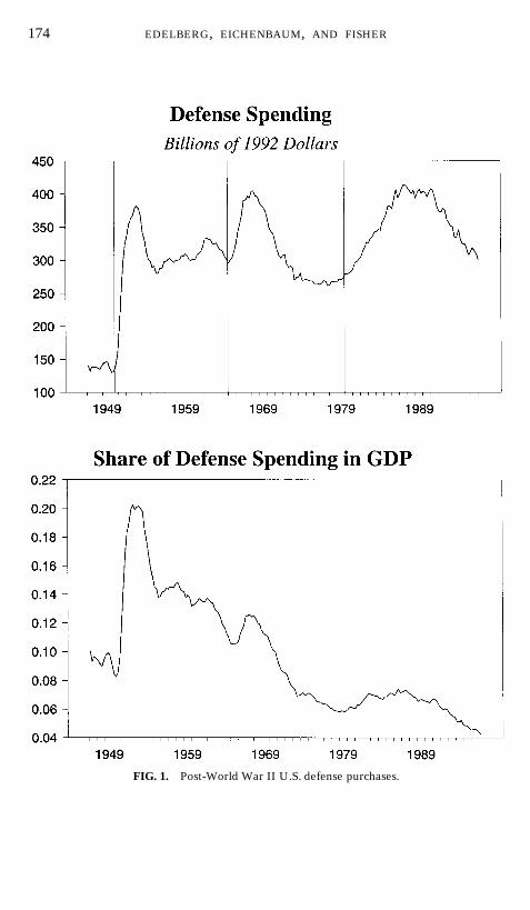
EDELBERG, EICHENBAUM, AND FISHER174
FIG. 1. Post-World War II U.S. defense purchases.
SHOCK TO GOVERNMENT PURCHASES 175
Reagan defense buildup. The Ramey]Shapiro dummy variables essentiallymark the beginning of these episodes.
The four panels of Fig. 2 report the responses of real defense spending,real government purchases, real GDP, and real private GDP to a Ramey]Shapiro episode. Here government purchases refers to defense spendingplus local, state, and federal government purchases of consumption goods.In Figs. 2]11 the solid lines display point estimates of the coefficients ofthe dynamic response functions.11 The dashed lines correspond to 68%confidence interval bands.12
Ž .Consistent with results of Ramey and Shapiro 1997 , the onset of aRamey]Shapiro episode leads to a large, persistent, hump-shaped rise indefense expenditures: g initially rises by about 1%, with a peak responsetof 30% roughly 6 quarters after the shock. The response of real govern-ment purchases is similar to that of real defense purchases. While theresponse is smaller, it is still substantial: total government purchases risein a hump-shaped pattern with a peak response of 14% roughly 6 quartersafter the shock. Paralleling the response of defense expenditures, there isa delayed, hump-shaped response in real GDP, with a peak response of
Žabout 3.5% 4 quarters after the shock. The rise in private real GDP GDP.minus government purchases is must smaller, with a peak response of
about 1.8%.Figure 3 displays the responses of various measures of employment to a
Ramey]Shapiro episode. Notice that private employment rises in a hump-shaped pattern which parallels the hump-shaped rise in defense andgovernment purchases. The response of employment in the manufacturingsector is qualitatively similar to the response of total private employment,but is larger, with a peak rise of roughly 5%. Employment rises in both thedurables and nondurables manufacturing sectors, with the rise in the firstsector exceeding the rise in the second sector. Finally, Fig. 3 indicates the
11 With one exception, the impulse response functions are reported in units of percentagepoint deviations from a variable’s unshocked path. The exception is that impulse response
Ž .functions of interest rates are reported in percentage points see Subsection 3.1.3 .12 These were computed using a bootstrap Monte Carlo procedure. Specifically, we
� 4Tconstructed 500 time series on the vector Z as follows. Let u denote the vector ofˆt t ts1residual from the estimated VAR. We constructed 500 sets of new time series of residuals,� Ž .4T � Ž .4Tu j , j s 1, . . . , 500. The t th element of u j was selected by drawing randomly,ˆ ˆt ts1 t ts1
� 4T � Ž .4Twith replacement, from the set of fitted residual vectors, u . For each u j , weˆ ˆt ts1 t ts1� Ž .4Tconstructed a synthetic time series of Z , denoted Z j , using the estimated VAR andt t ts1
� Ž .4Tthe historical initial conditions on Z . We then reestimated the VAR using Z j and thet t ts1historical initial conditions, and calculated the implied impulse response functions forj s 1, . . . , 500. For each fixed lag, we calculated the 80th lowest and 420th highest values ofthe corresponding impulse response coefficients across all 500 synthetic impulse responsefunctions. The boundaries of the confidence intervals in the figures correspond to a graph ofthese cofficients.

EDELBERG, EICHENBAUM, AND FISHER176
FIG. 2. Responses of government purchases and output.
employment in the construction sector and employment by the federalgovernment rise.
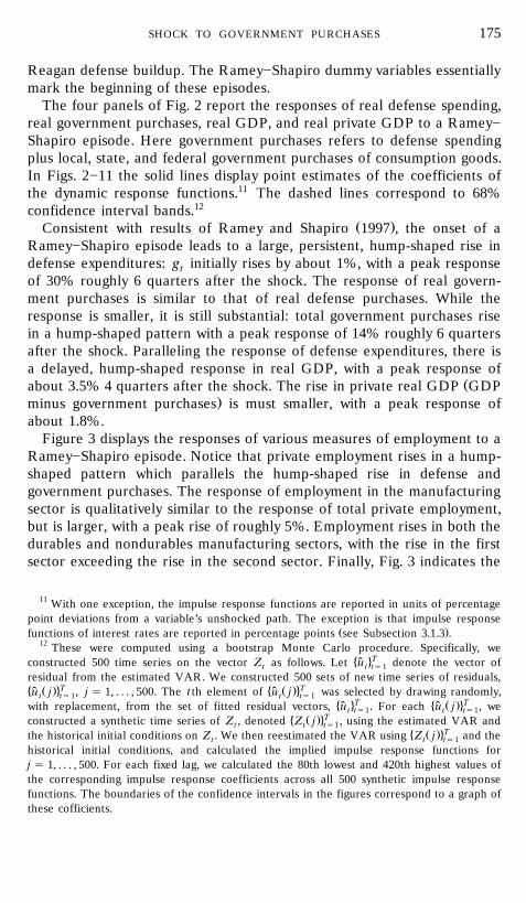
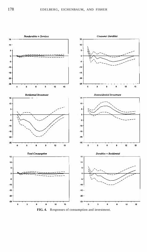
Figure 4 displays the response of real expenditures on different cate-gories of consumption and investment to a Ramey]Shapiro episode. Anumber of important results emerge here. First, consumption expenditures

SHOCK TO GOVERNMENT PURCHASES 177
FIG. 3. Responses of employment.
EDELBERG, EICHENBAUM, AND FISHER178
FIG. 4. Responses of consumption and investment.

SHOCK TO GOVERNMENT PURCHASES 179
FIG. 5. Responses of different types of nonresidential investment.

EDELBERG, EICHENBAUM, AND FISHER180
FIG. 6. Sectoral output responses.
SHOCK TO GOVERNMENT PURCHASES 181
FIG. 7. Responses of real labor compensation.

EDELBERG, EICHENBAUM, AND FISHER182
FIG. 8. Average marginal tax rates.
on nondurable goods and services fall after a brief delay. However, theresponse at all horizons is quite small. Second, there is an initial 6% rise inconsumption expenditures of durable goods. However, the expendituresquickly fall below their preshock levels. After 2 years, they are roughly 5%below their preshock level. The combined response of total real consump-tion expenditures on nondurables, services, and durables, depicted in thepanel labeled Total Consumption, is small.
To fully understand the response of consumption, we now consider howinvestment responds to Ramey]Shapiro episode. Figure 4 shows that apositive shock to government purchases is followed by a sharp decline inresidential investment. The peak response occurs roughly 6 quarters afterthe shock, at which point residential investment is 15% below its preshock
SHOCK TO GOVERNMENT PURCHASES 183
FIG. 9. Responses of real wages.

EDELBERG, EICHENBAUM, AND FISHER184
FIG. 10. Responses of different measures of manufacturing.

SHOCK TO GOVERNMENT PURCHASES 185
FIG. 11. Responses of money, prices, and interest rates.

EDELBERG, EICHENBAUM, AND FISHER186
level. Since residential investment and durable consumption purchasesboth represent investments in stocks of capital which yield consumptionservices, it is natural to consider the combined response of these types ofexpenditures. From the panel labeled Durables q Residential, we see thatthis combination of expenditures initially rises, but within 2 quarters it fallsbelow its preshock level. The peak response occurs roughly 2 years afterthe shock, with expenditures falling roughly 6% relative to their preshocklevel. Evidently, once we treat investment in housing symmetrically withinvestment in other consumer durables, there is substantial evidence of adecline in consumption-related expenditures.
In sharp contrast to residential investment, Fig. 4 shows that a Ramey]Shapiro episode leads to a persistent rise in nonresidential investment.The peak response occurs roughly 6 quarters after the shock, at whichpoint nonresidential investment expenditures are approximately 8% abovethe preshock level. Given the stark difference in the response paths ofresidential and nonresidential investment, it is important to understandwhich components of the latter rise. Fig. 5 indicates that all types ofnonresidential investment}information-processing equipment, structures,industrial equipment, producer durable equipment, and transportationequipment}rise in response to a Ramey]Shapiro episode.13
We conclude from studying Figs. 4 and 5 that a positive shock togovernment purchases induces a broad-based expansion in nonresidentialinvestment along with a delayed fall in consumption expenditures. Thelatter occurs mostly via a reduction in durable consumer good expendi-tures, defined to include investment in housing. Figure 6, which displays
Ž .the response of different measures of industrial production IP to aRamey]Shapiro episode, provides corroborating evidence for this view.First, the shock leads to persistent rise in manufacturing IP. The rise isconcentrated in durable manufacturing goods, which increase more sharplythan output of nondurables manufacturing goods. Consistent with theexpenditure data, we see an initial rise in the output of both durable andnondurable consumer goods. However, the increase is small and short-livedrelative to the rise in total manufacturing and durable goods manufactur-ing output. Both durable and nondurable consumer goods fall after about3 quarters, with the peak decline in the former exceeding that the latter.
3.1.2. Compensation and Real Wages
In this subsection we summarize our evidence regarding the response ofcompensation and real wages to a Ramey]Shapiro episode. As discussedin the Introduction, these results are particularly useful for assessing the
13 After roughly 6 quarters of investment in transportation, equipment begins to declinesignificantly.

SHOCK TO GOVERNMENT PURCHASES 187
empirical plausibility of alternative business cycle models. The key resultin the subsection is that every measure of compensation and real wagesthat we consider falls in response to a positive shock to governmentpurchases. This constitutes a strong challenge to claims in the literaturethat real wages rise in response to an exogenous increase in government
Ž .purchases see, for example, Rotemberg and Woodford, 1992 . In contrast,this result is consistent with neoclassical models which predict that realwages should go down after such a shock because of the negative incomeeffects associated with increases in government purchases.
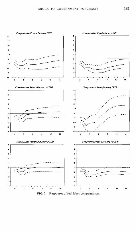
Figure 7 reports the estimated response functions for six measures ofŽreal compensation: compensation per hour in private business deflated by
.the CPI, a deflator for private business output and the GDP deflator andŽmanufacturing deflated by the CPI, the PPI for manufacturing, and the
.GDP deflator . Note that all six measures of compensation decline. In allcases, the fall in manufacturing compensation exceeds the correspondingfall in private business sector compensation.
Next we consider the response of real wages to a Ramey]Shapiroepisode. We do so using both before-tax and after-tax versions of variousreal wage measures. Our data on average marginal tax rates are based onthe annual tax rates for all sources of income reported by Fairlie and
Ž .Meyer 1996 . These are displayed in Fig. 8. In using this data, we assumethat tax rates are constant within the year that they apply to labor income.Note that the tax rate rises around each of the Ramey]Shapiro episodes.Consequently, working with before-tax real wages could in principle givemisleading results regarding firms’ and households’ incentives to varyemployment in the aftermath of a shock to government purchases.
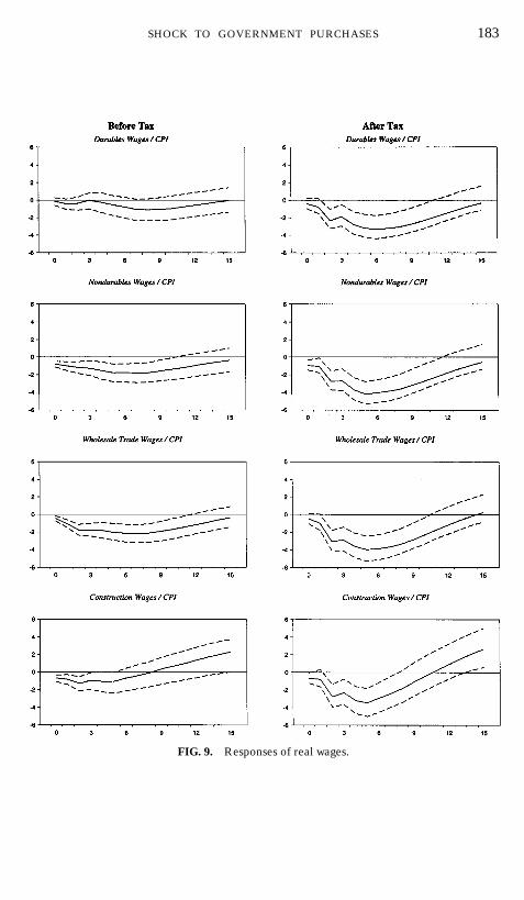
Figure 9 displays the response of eight measures of real wages to aRamey]Shapiro episode: before- and after-tax real wages in the durablesgoods manufacturing, nondurable goods manufacturing, wholesale trade,and construction sectors. Nominal wages are deflated using the CPI.14 Thekey result here is that every measure of the real wage falls after a positiveshock to government purchases. As expected, the fall in after-tax wages islarger than the fall in before-tax wages.
Figure 10 displays additional evidence regarding the response of realwages to a Ramey]Shapiro episode. Here we display the response func-tions of before- and after-tax real wage rates in the manufacturing sector,calculated using the CPI, the PPI for manufacturing, and the GDPdeflator. Consistent with Figure 9, each measure of the real wage fallsafter a positive shock to government purchases. Again the fall is larger forafter-tax wages.
14 Our results are very similar if we deflate using the GDP deflator. We could not obtainseparate PPI deflators for all of these industries.
EDELBERG, EICHENBAUM, AND FISHER188
Viewed overall, the evidence presented in this subsection strongly sup-ports the view that real wages fall in response to a positive shock togovernment purchases.
3.1.3. Prices, Money, and Interest Rates
In this subsection, we summarize our evidence regarding the behavior ofreal interest rates following a Ramey]Shapiro episode. As background forour discussion, column 1 of Fig. 11 presents the response functions for theGDP deflator, the CPI, and M1. Note that after a positive shock togovernment purchases, there is a persistent increase in all three variables.The peak response in M1 occurs roughly a year after the initial shock,while the peak responses in the GDP deflator and the CPI occur 1 or 2quarters earlier. Additional background is provided by column 2 of Fig. 11,which displays the response of three nominal interest rates: the yield on3-month, 1-year, and 2-year Treasury bills. In all three cases, the interestrate initially falls, but then rises.15
To examine the behavior of the real interest, we proceeded as follows.Define the j period ahead real interest rate, r , at time t, ast, j
r s R y E P y P . 5Ž .Ž .t , j t , j t tqj t
Here R is the log of the nominal yield on a j quarter bond purchased att, jtime t, P is the log of the CPI at time period t q j, and E denotes thetq j ttime t conditional expectation operator, which we compute using theestimated VAR.
Column 3 of Fig. 11 displays the dynamic response functions of thismeasure of the real interest rate for the 1-quarter rate, the 1-year rateŽ . Ž .j s 4 , and the 2-year rate j s 8 . Note that the real 1-quarter rate fallssharply for about 1 year before rising above its preshock level. The real1-year interest rate’s response is similar to that of the 1-quarter rate,except for a smaller initial decline. The 2-year rate rises more quickly thanthe 1-year rate, and the rise is larger.
Viewed overall, our results provide mixed evidence on the response ofthe real interest rate to an increase in government purchases. With abouta 1-year delay, all of our real interest rate measures rise after the onset ofa Ramey]Shapiro episode. However, substantial care must be taken ininterpreting this result. The k period ahead response of r depends ont, jthe expected rate of inflation from k periods after the shock to k q jperiods after the shock. In considering the response of the 2-year interestrate 1 year after the shock, inference depends critically on the ability to
15 These response functions were computed substituting the relevant interest rate into theVAR in place of the net 3-month Treasury bill rate used in the rest of our analysis.

SHOCK TO GOVERNMENT PURCHASES 189
reliably estimate the change in the price level between 1 year after theshock and 3 years after the shock. To the extent that there is bias in theVAR coefficients that push us away from unit roots in the price level, thiswould seriously affect inferences about the response of the price levelmany periods after the shock. In light of this, we view our interest rateresults as suggestive but hardly definitive.
3.2. Assessing the Robustness of Our Results
In the previous subsection we displayed estimates of the dynamic re-sponse of the U.S. economy to an exogenous change in governmentpurchases. There are at least two sources of uncertainty regarding theseresults. The first is due to sampling uncertainty in the estimated impulseresponse functions. This source of uncertainty is summarized by theconfidence interval bands displayed in the figures discussed above. Thesecond, which we investigate here, is due to uncertainty about the actualdates at which the Ramey]Shapiro episodes began.
The Monte Carlo methods that we used to quantify the importance ofsampling uncertainty do not convey any information about ‘‘date’’ uncer-tainty. This is because they take as given the Ramey]Shapiro dates. Onesimple way to assess the importance of date uncertainty is to redo ouranalysis perturbing the Ramey]Shapiro dates. We say that date uncer-tainty is not important if qualitative inference is robust to small perturba-tions in the Ramey]Shapiro dates. At the same time, if we obtained thesame results regardless of which dates we use in the analysis, we wouldlose confidence in our interpretation of the results. After all, if it does notmatter which dates we use, there would be no reason to interpret theestimated response functions as capturing the effects of an exogenousincrease in government purchases per se.
To assess the robustness of inference to perturbations in the Ramey]� 4Shapiro dates 1950:3, 1965:1, 1980:1 , we conducted the following three
experiments.
v Experiment 1: Hold the last two Ramey]Shapiro dates fixed. Thenredo the analysis of Section 3.1 assuming the actual date of the firstepisode was 1950:3 q j, j s y1, y2, y3, q1, q2, q3.
v Experiment 2: Redo experiment 1, but hold the first and thirdRamey]Shapiro dates fixed and perturb the second date.
v Experiment 3: Redo experiment 1, but hold the first two dates fixedand perturb the third date.
Figure 12 and 13 report the result of experiment 1 for a subset of theaggregates discussed in the previous section: real GDP, residential invest-
Žment, nonresidential investment, after-tax manufacturing wages calcu-

EDELBERG, EICHENBAUM, AND FISHER190
FIG. 12. Sensitivity to positive changes in Ramey]Shapiro dating of the Korean Warepisode.

SHOCK TO GOVERNMENT PURCHASES 191
FIG. 13. Sensitivity to negative changes in Ramey]Shapiro dating of the Korean Warepisode.
EDELBERG, EICHENBAUM, AND FISHER192
.lated using the CPI , nondurables and services consumption, and totalgovernment purchases. As can be seen, the effect of date uncertaintyregarding the first episode is quite small. Figure 12 reports estimatedimpulse response functions for nonnegative values of j. The only sensitivi-ties that emerge are as follows. First, if we assume that the Korean Warepisode actually began in 1951:2, after-tax manufacturing real wages fall,but with a 3-quarter lag. Second, the delayed small decline in nondurablesand services that occurs when j s 0 becomes a small rise for the othervalues of j. Still, the basic result regarding nondurables and services isrobust: the estimated response is small, regardless of which value of j isused. Figure 13 reports estimated impulse response functions for nonposi-tive values of j. Again, two sensitivities emerge. First, if we assume thatthe Korean War episode actually began in 1949:4, residential investmentrose in response to the military buildup. Second, when j is not equal tozero, there is small rise in nondurables and services after the increase ingovernment purchases.
Based on this evidence, we conclude that qualitative inference is robustup to misdating of the Korean War episode by 1 half-year in eitherdirection of the Ramey]Shapiro date. In the interests of space we do notreport analogs to Figs. 12 and 13 for experiments 2 and 3. This is becausethe estimated impulse response functions were extremely robust to varia-tions in j. In part this reflects the importance of the Korean War episodein generating our results.
3.3. Are the Ramey and Shapiro Episodes Special?
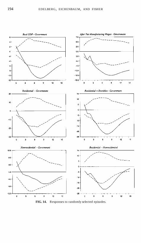
This subsection provides evidence on the response of the economy toRamey]Shapiro episodes relative to other, arbitrarily selected time peri-ods.16 For the sake of concreteness we focus on the response of real GDP,residential investment, nonresidential investment, after tax manufacturingwages and residential investment plus durable expenditures. We considerthe responses of these variables relative to government purchases toemphasize the conditional comovements with government purchases thatare induced by the onset of a Ramey]Shapiro episode. In addition, we findit of interest to consider the response of residential minus nonresidentialinvestment.
We proceeded as follows. First, we randomly chose three dates in oursample period, which we refer to as synthetic episode dates. Second, we
16 The Ramey]Shapiro dates enter the VARs in a statistically significant manner. Inparticular, the null hypothesis that the coefficient on the dummy variable associated withthese dates in zero can be rejected at the 1% significance level. However, this result does notbear directly on whether impulse response functions associated with the Ramey]Shapirodates are unusual, relative to those associated with other dates.

SHOCK TO GOVERNMENT PURCHASES 193
estimated the dynamic response of the variable in question to the onset ofa synthetic episode date, using the same methods that were used to
Ž .estimate the response to a Ramey]Shapiro episode see Section 2 . WeŽ .repeated this procedure 500 times sampling dates with replacement and
calculated the 25th lowest and 475th highest values of the correspondingimpulse response coefficients across the 500 impulse response functions.These are reported as dashed lines in Fig. 14, along with our pointestimate of the dynamic response function of the relevant variable ob-tained using the original Ramey]Shapiro dates. If there was nothingspecial about the pattern of comovements associated with the Ramey]Shapiro dates, then the estimated impulse responses to those dates oughtto lie within the dashed lines.
Notice that for every variable, the estimated response function liesoutside the confidence intervals for a subset of the horizons considered.Because this result was marginal in the case of nonresidential investment,we redid the analysis, focusing on residential minus nonresidential invest-ment. As can be seen, the estimated response function of this variable lieswell outside the confidence intervals for a broad subset of the horizonsconsidered. We conclude that the behavior of residential investmentrelative to nonresidential investment after the onset of a Ramey]Shapiroepisode is unusual, relative to other dates in the sample.
Based on this evidence we reject the view that the estimated responsefunctions discussed in Section 3.1 could have plausibly arisen from arbi-trarily selected dates for the time dummy variables. There is somethingspecial about the Ramey]Shapiro dates. In our view what is special is thatthey coincide with the onset of exogenous increases in government pur-chases.
4. ACCOUNTING FOR THE FACTS
In the previous section we attempted to document the response of theeconomy to an exogenous increase in government purchases. In thissection we interpret our findings using a simple modified version of theone-sector neoclassical growth model. The section is divided into threeparts. The first subsection describes our theoretical framework, the secondsubsection describes the way we calibrated the model’s parameters, andthe third subsection discusses the quantitative properties of our model.
4.1. Theoretical Framework
The model which we consider is a variant of the neoclassical growthmodel modified to allow for both nondurable and durable consumptiongoods. A representative household ranks alternative streams of consump-
EDELBERG, EICHENBAUM, AND FISHER194
FIG. 14. Responses to randomly selected episodes.
SHOCK TO GOVERNMENT PURCHASES 195
tion services and hours worked according to
`UtE b log C q h log 1 y n . 6Ž . Ž .Ý0 t t
ts0
Here E is the time 0 conditional expectations operator, b is a subjective0discount factor between 0 and 1, and CU and n denote time t consump-t ttion services and the fraction of the household’s time endowment devotedto work, respectively.
Consumption services are produced according to the technology:
1rcc c¡ u C q 1 y u D , c F 1, c / 0,Ž .t tU ~C s 7Ž .t u 1yu¢C D , c s 0,t t
where 0 F u F 1. The variable C denotes time t units of the nondurabletconsumption good, and D is the stock of durable consumption goods,twhich includes the stock of housing. Our decision to model housingtogether with other durable consumption goods is motivated by threeconsiderations. First, housing is a durable consumption good. Second, asFig. 4 shows, both residential investment and durable consumption goodexpenditures fall after the onset of a Ramey]Shapiro episode, althoughthe latter does so with a delay. Finally, for simplicity we thought itworthwhile to assume that the service flows from different durable goodsare perfect substitutes in consumption.
The aggregate resource constraint for the economy is given by
1yaa w xC q I q I q G F K X n , 0 - a - 1. 8Ž .t D , t K , t t t t t
Here K denotes the beginning of time t stock of market capital, Gt tdenotes time t government purchases, I denotes time t investment inK , tmarket capital, I denotes time t investment in household durable goods,D , tand X represents the time t state of technology. Throughout we assumetthat government purchases are financed by lump-sum taxes.
The stocks of market capital and durable consumption goods evolveaccording to
K s 1 y d K q I , 0 F d - 1,Ž .tq1 K t K , t D9Ž .
D s 1 y d D q I , 0 - d - 1.Ž .tq1 D t D , t K
Ž . Ž .Relation 8 and the second equation in 9 embed the assumption, madefor simplicity, that the technology used to produce housing stocks and thatused to produce other consumer durable goods are identical.

EDELBERG, EICHENBAUM, AND FISHER196
Technology evolves in the following deterministic fashion:
X s g t , g G 1, 10Ž .t
while government purchases evolve according to
G s X g . 11Ž .t t t
Ž . Ž .We assume that log g has a finite ordered ARM A p, q representation:t
A L log g s B L e , 12Ž . Ž . Ž . Ž .t t
Ž . Ž .where A L and B L are finite ordered polynomials in nonnegativeŽ .powers of the lag operator L. The roots of A L are all assumed to lie
outside the unit circle, and « is an iid shock that is orthogonal to alltmodel variables dated time t y 1 and earlier.
It is convenient to define
C D Kt t tc s , d s , k s , 13Ž .t t tX X Xt t t
as well as
1rcc cu c , d , 1 y n s log u c q 1 y u d q h log 1 y n . 14Ž . Ž . Ž . Ž .t t t t t t
Under the assumption of perfect competition and complete markets, thecompetitive equilibrium allocation for our model economy is given by thesolution to the following planning problem. Maximize
`tE b u c , d , 1 y n 15Ž . Ž .Ý0 t t t
ts0
subject to
c q g d y 1 y d d q g k y 1 y d k q g s k an1ya , 16Ž . Ž . Ž .t tq1 D t tq1 K t t t t
Ž . Ž .12 and 14 . The maximization is by choice of contingency plans for� 4c , d , k , n over the elements of the planner’s time t informationt tq1 tq1 tset, which we assume includes all model variables dated time t and earlier.Given the solution to this problem, we can obtain the competitive equilib-
Ž . Ž .rium allocation for C , D , and K using 10 and 13 .t t tWe solve the model using the log linear approximation discussed by
Ž .Christiano 1998 . Given the competitive equilibrium quantity allocation,

SHOCK TO GOVERNMENT PURCHASES 197
the equilibrium real wage rate and one period ahead ex post interest rateare given by
a 1yaw s 1 y a X k rn and r s a n rk q 1 y d ,Ž . Ž . Ž . Ž .t t t t t , 1 tq1 tq1 K
17Ž .
respectively.
4.2. Model Calibration
In this subsection we briefly describe the way we calibrated the model’sŽ . y1r4parameters. Following Fisher 1997 , we set b s 1.03 , g s 1.004,
a s 0.237, d s 0.021, and d s 0.022. The parameter h was set to implyK Dthat in nonstochastic steady state the representative consumer spends 30%of his time endowment working. This yielded a value of h equal to 2.74. Toassess the robustness of our results, we considered three values of theparameter c , which controls the degree of substitutability between C andtD in the production of CU. For each value of c , we chose u so that thet tnonstochastic steady-state value of DrK equals 0.78. This is the sample
Žaverage of the corresponding number in the postwar U.S. data see Fisher,. 171997 . We report results for three values of c and corresponding values
of u :
c u
0 0.710.5 0.89
y1.0 0.16
Ž .The unconditional mean of the process log g was set of 0.117, whichtimplies a nonstochastic steady-state value of GrY equal to 0.21. This isequal to the average value of GrY over our sample period, where G is
Ždefined as total real defense purchases plus total real government federal,.state, and local nondefense consumption expenditures, and Y equals real
GDP. Given our parameter values, the nonstochastic steady-state values of
17 Ž .The analog number reported by Greenwood and Hercowitz 1991 in 1.13. The numbersŽ .differ because Greenwood and Hercowitz 1991 ignore government capital in their analysis.

EDELBERG, EICHENBAUM, AND FISHER198
the key stationary model variables are
CrY I rY I rY GrY nK D
0.46 0.18 0.15 0.21 0.30
To assess the empirical plausibility of our model, we compare itsresponse to an exogenous shock in G to the analog response functionstdiscussed in Section 3. To this end, we consider three parameterizations ofŽ . Ž .A L and B L , the first two of which are useful primarily for pedagogical
purposes.
Ž .Parameterization 1: Here log g is assumed to be iid:t
A L s 1, B L s 1. 18Ž . Ž . Ž .
Ž . Ž .Parameterization 2: Here we suppose that log g is an AR 1 process:t
A L s 1 y 0.9L, B L s 1. 19Ž . Ž . Ž .
Parameterization 3: While parameterizations 1 and 2 are useful forunderstanding the dynamic properties of our model, they are not useful forassessing its empirical plausibility. This is because the actual response pathof G induced by a shock to government purchases is inconsistent with thet
Ž . Ž .paths implied by 18 and 19 . One way to ensure such consistency is toŽ .assume that log g evolves according to a univariate moving averaget
representation whose coefficients are given by the estimated dynamicresponse function for a Ramey]Shapiro episode.18 Note that this repre-sentation is valid only for assessing the ability of the model to account forthe response of the economy to an exogenous shock to governmentpurchases. In particular, it would be inappropriate to compare the uncon-ditional second moment properties of the model under this representation
Ž .for log g to the unconditional second moments of the data.tWith the previous considerations in mind, we adopt as our third parame-
terization
A L s 1,Ž .B : estimated response of real government purchases at t q jj 20Ž .
to the onset of a Ramey]Shapiro episode at time t .
18 This claim can be established using arguments identical to those made by Christiano etŽ .al. 1997 with reference to monetary policy shocks.

SHOCK TO GOVERNMENT PURCHASES 199
The first 16 B coefficients that we used are depicted in the top row of thejsecond column of Fig. 2. In solving the model, we actually used the first 50coefficients of the estimated impulse response of real government pur-chases to the onset of a Ramey]Shapiro episode. Subject to specificationerror entailed in approximating an infinite ordered polynomial with afinite number of lags, this ensures that the experiment being conducted inthe model coincides with the experiment which we claim to have isolatedin the data. Consequently, if our model has been specified correctly, thedynamic consequences of a shock to government purchases should be the
Ž .same aside from sampling uncertainty in our model as in the data.
4.3. Quantitative Results
Figures 15, 16, and 17 summarize the dynamic response of our modelŽ . Ž .economy to a shock to government purchases when A L and B L are
Ž . Ž . 19given by 18 ] 20 , respectively. In the first two cases, we consider ashock equal to a 1% positive deviation of G from its nonstochastictsteady-state growth path. For the third case, the shock is equal to unity. In
Ž .each case we present results for c s 0, 0.5, y1.0 . To understand theseresults, recall that the key effect, in our model, of an increase in govern-ment purchases, is a decline in the representative household’s permanentincome.
In the case of the iid shock to government purchases displayed in Fig.15, this effect is very small. As a consequence, the shock has a very smalleffect on hours worked, the real wage rate, and the interest rate. Thehousehold wishes to smooth the flow of consumption services that it enjoysover time. Consistent with the results displayed in Fig. 15, the optimal wayto do this in the face of a small, transitory shock in income is to reduce
Ž .market investment I and investment in household durable goodsK , tŽ .I . By doing this the household can free up resources to minimize theD , tfall in nondurable consumption purchases. Since the flow of services fromdurables is determined by the stock of durables, it too falls by a relatively
Žsmall amount. It follows that total consumption services not displayed in.Fig. 15 falls by a relatively small amount. The optimal ratio of the decline
in nondurable and durable consumption services is determined by thevalue of c . Nevertheless, the qualitative features of the response functionsare very similar across the three values of c which we considered. Finally,it is worth emphasizing that a key feature of these response functions isthat, in the case of a small transitory positive shock to governmentpurchases, both I and I decline.K , t D , t
19 Note that the response labeled ‘‘Consumption’’ corresponds to purchases of nondurableconsumption goods, C , not consumption services, CU.t t

EDELBERG, EICHENBAUM, AND FISHER200
FIG. 15. Model-based impulse response functions: government purchases}IID.
Ž .Consider next Fig. 16, which corresponds to the case in which log g istŽ .an AR 1 process with AR coefficient equal to 0.9. Here the initial positive
shock to g is associated with a nontrivial decline in the household’stpermanent income. Since leisure is a normal good, equilibrium employ-ment rises. In the impact period of the shock, the stock of market capital isfixed. With employment up, the marginal product of labor falls and hence
Ž .real wages do also. Consistent with results of Aiyagari et al. 1992 , the

SHOCK TO GOVERNMENT PURCHASES 201
Ž .FIG. 16. Model-based impulse response functions: government purchases}AR 1 .
household finds it optimal to reduce consumption and increase marketinvestment. The easiest way to see the reason for the latter is to considerthe case of a permanent rise in government purchases. In this case thesteady-state value of hours worked rises. Given our other assumptions, the
Ž .steady-state value of krn does not change, so that k must rise. To buildup the higher steady-state stock of k, actual investment must initiallyexceed its new, higher steady-state value. The same basic forces apply in

EDELBERG, EICHENBAUM, AND FISHER202
FIG. 17. Model-based impulse reponse functions: government purchases]estimated mov-ing average representation.
the face of a persistent, but not permanent, increase in governmentpurchases. The household must work harder for a number of time periodsto pay its larger tax bill. Since hours worked and market capital arecompliments, the household initially increases I in response to theK , tshock. To reduce the flow of consumption services it enjoys, the householdreduces consumption of nondurables and the service flow from durable

SHOCK TO GOVERNMENT PURCHASES 203
goods. To accomplish the latter it reduces I . So, in response to aD , tpersistent increase in government purchases, I rises while I falls.K , t D , tRecall that this was a key feature of our empirical results.
It is interesting to note that the shock leads to a hump-shaped responsein hours worked as well as output. This reflects the fact that market capitaland hours worked are complements in production. The maximal rise inhours worked occurs after the extra capital induced by the rise in IK , tbecomes available. The hump-shaped pattern in hours worked and marketcapital generates a hump-shaped pattern in output. Finally, consistent with
Ž .results of Aiyagari et al. 1992 , the real interest rate rises, but by a verysmall amount.
Figure 17 depicts the response of the economy to a shock to governmentŽ . Ž .purchases given by our third parameterization of A L and B L . Notice
that Figs. 16 and 17 have very similar qualitative features. This is because,in our model, what is important about a shock to g is its impact on thetpresent value of household’s tax burden. This impact is larger for the thirdparameterization, and its effects are correspondingly larger. The qualita-tive effects on the model economy are very similar, however. So again, themodel can account for the fact that, in response to a persistent shock to g ,tconsumption, real wages, and I decline, while hours worked, output,D , tI , and the real interest rate rise.K , t
5. CONCLUSION
This paper analyzed the effect of a positive shock to real governmentpurchases on the U.S. economy. Consistent with results of Ramey and
Ž .Shapiro 1997 , we find that in response to such a shock, total governmentpurchases, employment, output, and nonresidential investment rise, whilereal wages, residential investment, and, after a slight delay, consumptionexpenditures on nondurable goods and services and durable goods fall.The negative response of real wages is particularly useful for discriminat-ing between alternative business cycle models. Models which stress theimportance of increasing returns to scale and imperfect competition pre-dict that a positive shock to government purchases drives real wages up. Incontrast, simple neoclassical growth models predict that real wages shouldfall in response to such a shock. Our findings cast doubt on the empiricalplausibility of the first class of models and provide support for the secondclass of models.
We also argued that a simple variant of the neoclassical growth modelcan account for the finding that residential investment falls while nonresi-dential investment rises in response to an increase in government pur-
EDELBERG, EICHENBAUM, AND FISHER204
chases. The key modification was to model residential investment as aform of investment in the stock of durable consumption goods.
While successful on a variety of dimensions, our model suffers fromimportant shortcomings. First, the model inherits the well-known inabilityof simple complete market representative consumer models to account forthe observed time series behavior of asset returns. These failures manifestthemselves here in the response of the real interest rate to a shock togovernment purchases. Roughly speaking, the model predicts that the realinterest rate is unaffected by a shock to government purchases. Second,the model-based dynamic response functions of residential and nonresi-dential investment do not exhibit the persistent, hump-shaped patternsthat characterize our estimated response functions. The second shortcom-
Ž .ing is reminiscent of the finding by Greenwood and Hercowitz 1991 thatreal business cycle models cannot account for some key features of thedynamic paths of household and business capital in response to an aggre-gate technology shock. It would be interesting to enrich our model byallowing for differential costs of adjusting residential and nonresidentialinvestment. It is possible, but far from certain, that plausible adjustmentcosts could remedy this aspect of the model’s shortcomings.
We conclude by noting a potentially important limitation of our analysis.There is clear evidence that average marginal tax rates on income rose
Ž .after the onset of the Ramey]Shapiro episodes see Fig. 8 . However, weevaluated our model under the assumption that taxes are lump sum innature. Allowing for a rise in marginal tax rates could very well affect theempirical performance of our model. This is because higher tax rateswould dampen the positive response of employment and output associated
Žwith increases in government purchases see, for example, Baxter and. Ž .King, 1993 . Indeed, results in Mulligan 1998 imply that in order to
understand the behavior of the U.S. economy during World War II, it isimportant to simultaneously take into account the large rise in marginaltax rates and government expenditures that occurred. An important set of
Ž . Žtasks that we leave to future research are i finding out which taxes e.g.,.labor versus capital income taxes rose after the Ramey]Shapiro episodes,
Ž . Ž .ii incorporating these into our model, and iii assessing the net effect ofan increase in government purchases when offsetting tax changes aretaken into account.
DATA APPENDIX
Our data are from four main sources. Below we list the series whichcorrespond to each of these sources. All series are seasonally adjusted,except for interest rates. Most of these series were obtained by us from theFederal Reserve Board’s macroeconomic database. Where possible, we

SHOCK TO GOVERNMENT PURCHASES 205
provide the mnemonic for the same series from the commercially availableDRI BASIC Economics Database.
Ž .1. Bureau of Economic Analysis. GDP GDPQ , defense spendingŽ . ŽGGFEQ , government purchases defense spending plus Federal, state,
. Žand local consumption expenditures GGFEQ q GGOCEQ q. Ž .GGSCPQ , private GDP GDP y government purchases , nondurable
Ž .goods and services consumption expenditures GCNQ q GCSQ , durableŽ . Žgoods consumption expenditures GCDQ , total consumption the sum of
. Ž .nondurables, services and durables expenditures GCQ , residential in-Ž . Ž .vestment GIRQ , nonresidential investment GINQ , nonresidential
structures investment, producer durable equipment investment, informa-tion-processing equipment investment, industrial equipment investment,
Ž .transportation equipment investment, GDP deflator GDPrGDPQ . Thequantity series are all in units of 1992 chain-weighted dollars, with theexception of the components of nonresidential investment, which are thechain-weighted quantity indexes. The latter were downloaded directly fromwww.stat-usa.gov.
Ž .2. Bureau of Labor Statistics BLS .
v Ž . Ž .Employment: Total private LP , manufacturing LPEM , con-Ž . Ž .struction LPCC , durable manufacturing LPED , nondurable manufac-
Ž . Ž .turing LPEN , federal government LPGOVF .v Compensation: real compensation per hour in business sector
Ž . Ž .LBCP7 , real compensation per hour in manufacturing sector LCPM7 .Note that these compensation series are the nominal compensation seriesdeflated by the BLS using the consumer price index for all urban con-sumers. We obtained the alternative real compensation series used in ouranalysis by inflating the BLS compensation series by the CPI and thendeflating by the indicated price series.
v Ž .Wages: Manufacturing LEHM , durable goods manufacturingŽ .LE67HMD, seasonally adjusted using the Census X-11 procedure , non-
Ždurable goods manufacturing LE6HMN, seasonally adjusted using the. Ž .Census X-11 procedure , wholesale trade LEHTW , construction
Ž .LEHCC .v Ž .Prices: Consumer price index for all urban consumers PUNEW ,
Ž .producer price index for the manufacturing sector PWM , private busi-Ž .ness deflator LBGDP , producer price index for crude fuel in manufactur-Ž .ing industries PW1310 .
3. Board of Governors of the Federal Reserve System. Net 3-monthŽ . Ž .Treasury Bill secondary market interest rate FYGM3 , M1 FM1 , indus-
Ž . Ž .trial production]manufacturing IPMFG , consumer goods IPC , durableŽ . Ž .manufacturing IPD , durable consumer goods IPCD , nondurable manu-
Ž . Ž .facturing IPN , nondurable consumer goods IPCN .

EDELBERG, EICHENBAUM, AND FISHER206
4. Robert Bliss, Federal Reserve Bank of Atlanta. Zero couponyields on 3-month, 1-year, and 2-year treasury securities.
REFERENCES
Ž .Aiyagari, R., Christiano, L., and Eichenbaum, M. 1992 . ‘‘The Output, Employment andInterest Rate Effects of Government Consumption,’’ Journal of Monetary Economics 30,73]86.
Ž .Baxter, M., and King, R. G. 1993 . ‘‘Fiscal Policy in General Equilibrium,’’ AmericanEconomic Re¨iew 83, 315]334.
Ž .Blanchard, O., and Perotti, R. 1998 . ‘‘An Empirical Characterization of the Dynamic Effectsof Changes in Government Spending and Taxes and Output,’’ manuscript, MIT, Cam-bridge, MA.
Ž .Burnside, C., and Eichenbaum, M. 1996 . ‘‘Factor Hoarding and the Propagation of BusinessCycle Shocks,’’ American Economic Re¨iew 86, 1154]1174.
Ž .Christiano, L. J. 1990 . Handout for comment on Oligopolistic Pricing and the Effects ofAggregate Demand on Economic Acti ity by J. Rotemberg and M. Woodford, NBEREconomic Fluctuations Meetings, Palo Alto, CA.
Ž .Christiano, L. J. 1998 . ‘‘Solving Dynamic Equilibrium Models by a Method of UndeterminedCoefficients,’’ NBER technical working paper no. 225.
Ž .Christiano, L. J., and Eichenbaum, M. 1992 . ‘‘Current Real Business Cycle Theories andAggregate Labor Market fluctuations,’’ American Economic Re¨iew 82, 430]450.
Ž .Christiano, L. J., Eichenbaum, M., and Evans, C. 1997 . ‘‘Monetary Policy Shocks: WhatŽHave We Learned and To What End?’’ in Handbook of Monetary Economics, Michael
.Woodford and John Taylor, Eds. .Ž .Christiano, L. J., Eichenbaum, M. and Evans, C. 1998 . ‘‘Modelling Money,’’ NBER working
paper no. 6371.Ž .Devereux, M. B., Head, A. C., and Lapham, M. 1996 . ‘‘Monopolistic Competition, Increas-
ing Returns, and the Effects of Government Spending,’’ Journal of Money, Credit, andBanking 28, 233]254.
Ž .Eichenbaum, M. 1997 . Comment on ‘‘Costly Capital Reallocation and the Effects ofGovernment Spending’’ by Valerie A. Ramey and Matthew D. Shapiro, in CarnegieRochester Conference on Public Policy.
Ž .Fairlie, R. W., and Meyer, B. D., 1996 . ‘‘Trends in Self-Employment among White andBlack Men: 1910]1990,’’ manuscript, Northwestern University.
Ž .Fisher, J. D. M. 1997 . ‘‘Relative Prices, Complimentarities and Comovement among Compo-nents of Aggregate Expenditures,’’ Journal of Monetary Economics 39, 449]474.
Ž .Greenwood, J., and Hercowitz, Z. 1991 . ‘‘The Allocation of Capital and Time over theBusiness Cycle,’’ Journal of Political Economy 99, 1188]1214.
Ž .Mulligan, C. 1998 . ‘‘Pecuniary and Nonpecuniary Incentives to Work in the US duringWorld War II,’’ manuscript, University of Chicago.
Ž .Ramey, V., and Shapiro, M. 1997 . ‘‘Costly Capital Reallocation and the Effects of Govern-ment Spending,’’ in Carnegie Rochester Conference on Public Policy.
Ž .Phelan, C., and Trejos, A. 1996 . ‘‘The Aggregate Effects of Sectoral Reallocation,’’manuscript, Northwestern University.
Ž .Rotemberg, J., and Woodford, M. 1992 . ‘‘Oligopolistic Pricing and the Effects of AggregateDemand on Economic Activity,’’ Journal of Political Economy 100, 1153]1297.