Notes on Linear Approximations, Equilibrium

Multiplicity and E-learnability in the Analysis of

the Zero Lower Bound�

Lawrence J. Christiano Martin Eichenbaum

March 12, 2012

�We are very grateful for discussions with Anton Braun, Luca Dedola, Giorgio Primiceri, and

Mirko Wiederholt. We are particularly grateful to Marco Bassetto for encouraging us to consider

E-learnability.

Abstract

We study the properties of the zero lower bound model in Eggertson andWood-

ford (2003) (EW). EW�s analysis is based on the equilibrium conditions after

linearization. Working with the actual nonlinear equilibrium conditions and

consistent with Braun, Körber and Waki (2012) and Mertens and Ravn (2011),

we �nd the existence of equilibria that are not visible to analyses based on lin-

earization, as well as sunspot equilibria. These �ndings challenge the �ndings

about the properties of the zlb reported in Christiano, Eichenbaum and Re-

belo (2011), Eggertson (2011), EW and others. However, we �nd that the

equilibria that are �invisible�to analyses using linearization are not E-learnable

and so those equilibria may perhaps be treated as mathematical curiosities.

In addition, evidence that the quality of linear approximations is poor rests

on examples where output deviates by more than 20 percent from its steady

state, cases where no one would expect linear approximations to work well. For

perturbations of reasonable size, the conclusions arrived at in the zlb analysis

that use linear approximations appear to be robust.

1. Introduction

In an in�uential paper, Eggertsson and Woodford (2003) (EW) studied an equilib-

rium for a simple New Keynesian model without capital in which the zero lower

bound on the nominal rate of interest (zlb) is binding. A well-chosen set of simpli-

fying assumptions on the environment greatly simpli�ed the analysis. EW studied

an equilibrium which is characterized by two numbers, in�ation and output when

the zlb binds, and two equations. In the equilibria they study, the system jumps

immediately to steady state as soon as the shock that makes the zlb bind goes away.

2

Because the equations are linearized, there is a unique solution.

The analysis is so in�uential in part because its simplicity permits a straightfor-

ward analytic derivation of a number of interesting results. These results include

(see, for example, EW, Eggertsson (2011) and Christiano, Eichenbaum and Rebelo

(2011) (CER)):

� When the zlb binds, the loss in output is potentially substantial.

� The output multiplier on government consumption is larger when the zlb binds

than when it does not bind.

� When prices are more �exible, or the expected duration of the zlb is longer, then

the magnitude in the drop in output in the zlb is greater and the government

consumption multiplier is larger.

In this paper, we restrict ourselves to the type of equilibria considered in EW.

That is, we consider equilibria in which the system jumps to a particular steady

state as soon as the shock is over. In addition, equilibrium while the zlb binds

is characterized by constant numbers. We depart from EW by not linearizing the

equilibrium conditions. We do this using the strategy followed in Braun, Körber

and Waki (2012), who interpret the price frictions in the EW analysis as stemming

from adjustment costs as proposed by Rotemberg (1982). This interpretation is

interesting because it implies the same linearized equations that EW study. An

alternative approach which also implies the linearized equations studied by EW is

based on the price setting frictions proposed by Calvo. The advantage of adopting

Rotemberg adjustment costs here is analytic simplicity. The Calvo approach injects

an endogenous state variable (past price dispersion), while there is no endogenous

state variable in the Rotemberg approach.

3

We �nd that the key qualitative results listed above survive our nonlinear analy-

sis. Our argument takes the following form. First, as in Braun, Körber and Waki

(2012) we �nd that there are multiple equilibria, including the sunspot equilibrium

documented in Mertens and Ravn (2011). If we look across all the equilibria, one can

argue that the conclusions described in the bullets above are not robust.1 For ex-

ample, in the sunspot equilibrium the government consumption multiplier is smaller

when the zlb binds than when it does not bind. This �atly contradicts a key claim

in the literature. Second, we impose the requirement that equilibria be E-learnable.

Subject to this re�nement the model has a unique equilibrium. Third, the properties

of the unique equilibrium have the properties stressed in the existing zlb literature.

A caveat to our results is that E-learnability requires taking a stand on a learn-

ing mechanism. We are currently exploring alternative learning mechanisms and

re�nement criteria.

Section 2 below describes our model. Section 3 discusses model steady states and

relates our analysis to that of Benhabib, Schmitt-Grohe and Uribe (2001). Section

4 de�nes the set of equilibria that we study. Section 5 derives the linearized equi-

librium conditions of the model. This establishes a baseline for comparison. Section

6 discusses E-learnability and describes the learning rule that we employ. Section

7 presents our results for EW equilibria. Finally, section 8 reviews the sort of cal-

culations that are done when researchers wish to go beyond qualitative results used

to develop intuition about the properties of economies in the zlb. In practice, those

researchers often apply deterministic simulation methods. We investigate the qual-

ity of the of the linear approximations within that context. Conclusions appear in

section 9.1It is not even clear how one de�nes a multiplier when there are multiple equilibria. Before and

after the jump in G there are two sets of equilibria.

4

2. Model

A representative household maximizes

E0

1Xt=0

�thlog (Ct)�

�

2h2t

isubject to

PtCt +Bt � (1 +Rt�1)Bt�1 +Wtht +�t;

where �t represents lump-sum pro�ts net of lump-sum government taxes. The �rst

order necessary conditions associated with an interior optimum are:

�htCt =Wt

Pt;

1

1 +Rt= �Et

PtCtPt+1Ct+1

:

Aggregate output, Yt; is produced by representative, competitive �nal good pro-

ducer using intermediate goods, Yjt; j 2 [0; 1] : The production function and �rst

order conditions are:

Yt =

�Z 1

0

Y"�1"

j;t dj

� ""�1

; " � 1; Yj;t =�Pj;tPt

��"Yt:

Each intermediate good is produced by a monopolist. The monopolist that produces

the jth good has the following objective:

Et

1Xl=0

�l�t+l[(1 + �)Pj;t+lYj;t+l �labor costs of productionz }| {st+lPt+lYj;t+l

�

cost (in terms of �nal goods) of adjusting prices related to aggregate level of outputz }| {�

2

�Pj;t+lPj;t+l�1

� 1�2(Ct+l + Gt+l) � Pt+l];

where �t denotes the state and date-contingent value assigned to payments sent to

households. When = 1; then adjustment costs in changing prices are related to

aggregate GDP, Ct +Gt; and when = 0 they are related to the level of household

5

consumption only. We also allow for intermediate cases, because it is not clear on a

priori grounds which speci�cation is more sensible. Finally, � is a subsidy to �rms

to address distortions due to monopoly power. We assume

1 + � ="

"� 1 :

The jth intermediate good producer takes the �rst order condition of the rep-

resentative �nal good producer as its demand curve. The production function and

level of �rm marginal cost (excluding costs associated with price changes) are given

by:

Yj;t =

production functionz}|{hj;t ; st �

real marginal costz}|{Wt

Pt=

household optimizationz }| {�htCt

The �rm is required to satisfy whatever demand occurs at its posted price, so that

we can substitute out for Yjt using the �rm�s demand curve. Doing this and imposing

�t = 1=(PtCt):

maxfPj;lg1

l=0

Et

1Xl=0

�l1

Pt+lCt+l[(1 + �)Pj;t+l

�Pj;t+lPt+l

��"Yt+l

�Pt+lst+l�Pj;t+lPt+l

��"Yt+l �

�

2

�Pj;t+lPj;t+l�1

� 1�2

Pt+l (Ct+l + Gt+l)]:

The �rst order condition is, after rearranging:

(1 + �)Pj;tPt

="

"� 1st + (2.1)

�1

"� 1

�Pj;tPt

�"CtYt[��

Pj;tPj;t�1

� 1�

Pj;tPj;t�1

(Ct + Gt)

Ct

+�Et

�Pj;t+1Pj;t

� 1�Pj;t+1Pj;t

�Ct+1 + Gt+1

Ct+1

�]

When � = 0; the jth �rm simply sets price, Pj;t; to a markup, "= ("� 1) ; over

marginal cost. If that price is high relative to yesterday�s price, then the �rm raises

6

Pj;t by less if � > 0; according to the �rst term in square brackets. Similarly, the

second expression in square brackets implies that if that price is low relative to next

period�s price, then the �rm raises price by more if � > 0: Impose the equilibrium

condition, Pj;t = Pi;t = Pt for all i; j; and rearrange:

(�t � 1)�t =1

�

��1 + � � "

"� 1

�(1� ") + " (st � 1)

�Yt

Ct + Gt

+�Et (�t+1 � 1)�t+1(Ct+1 + Gt+1)

Ct+1

CtCt + Gt

:

We adopt the assumption that a su¢ cient subsidy is provided to intermediate goods

producers so that, at least in steady state, the monopoly distortion is eliminated:

1 + � � "

"� 1 :

There are three uses of gross �nal output: household and government consump-

tion, and goods used up in changing prices:

Ct +Gt +�

2(�t � 1)2 (Ct + Gt) � Yt:

In equilibrium, this is satis�ed as an equality because households and government

go to the boundary of their budget constraints. Government consumption is an

exogenous process discussed below.

The four equilibrium conditions associated with the four unknowns, �t; Ct; Rt; ht;

are:

7

1

Rt=

1

1 + rtEt

Ct�t+1Ct+1

(2.2)

(�t � 1)�t =1

�" (st � 1)

YtCt + Gt

(2.3)

+1

1 + rtEt (�t+1 � 1)�t+1

(Ct+1 + Gt+1)

Ct+1

CtCt + Gt

(2.4)

Ct +Gt +�

2(�t � 1)2 (Ct + Gt) = ht (2.5)

Rt = max

�1;1

�+ � (�t � 1)

�: (2.6)

The last equation is the monetary policy rule.

We suppose that rt 2�rl; rh

. The economy starts with rt = rl in the initial

period; and it jumps to rh (� 1=� � 1) with constant probability 1� p: With prob-

ability p; the discount rate remains at its initial, low, value. The higher level, rh; is

an absorbing state for rt. There are no other stochastic shocks in the system. We

consider two types of equilibria. In one, rl < 0 and rh > 0:We call this a �fundamen-

tal equilibrium�, because the shock a¤ects preferences. We also consider a sunspot

equilibrium, in which rl = rh; so that the uncertainty does not a¤ect preferences or

technology.

3. Model Steady States

Given our assumption about the exogenous shock process, the exogenous randomness

settles down eventually in its absorbing state. As a result, the model has a well

de�ned steady state. Benhabib, Schmitt-Grohe and Uribe (2001) drew attention

to the fact that a model economy like ours has two steady states. They created

a diagram, Figure 1, that makes this particularly clear. Two of the equilibrium

conditions of the model include the monetary policy rule and the steady state version

8

of the intertemporal Euler equation:

R = max

�1;1

�+ � (� � 1)

�R = �=�;

respectively. Figure 1 shows that the above two equations have two crossings. The

two steady states involve � = 1 and � = �: Once the in�ation rate is selected, then

the Phillips curve and aggregate output relations can be used to determine steady

state C and h :

(� � 1)� =1

�" (�Ch� 1) h

C + G+ � (� � 1)�

C +G+�

2(� � 1)2 (C + G) = h:

Our baseline parameters are:

G = 0:20; � = 0:99; "=� = 0:03; � = 100; � = 1:25; = 0:

When steady state � = �; then C = 0:7971 and h = 1:001: When the steady state

is � = 1; then C = 0:80 and h = 1: The di¤erence is quite small. From here

on, we follow EW in assuming that when the shock switches to its high value, the

economy jumps to the higher of the two steady states. One rationale for selecting

this steady state may be that the monetary policy rule is actually composed of the

Taylor rule with an escape clause which speci�es that if in�ation is not proceeding

at its target rate (i.e., in�ation is negative versus its target value of zero) then the

money growth rate is adjusted. Fleshing out this argument, of course, must be done

by introducing money demand and supply. However, with enough separability, this

can be done without changing the equilibrium conditions that we work with here

(see, for example, Christiano and Rostagno (2001)).

9

4. An Interior, EW Equilibrium

An interior EW equilibrium is a set of eight numbers:

�h; Ch; Rh; hh; �l; C l; Rl; hl;

that satisfy the equilibrium conditions for the two values of the exogenous shock, �h�

for when rt = rh and �l�for when rt = rl. In the low state:

1

Rl=

1

1 + rl

�pC l

�lC l+ (1� p)

C l

�hCh

�(4.1)

��l � 1

��l =

1

�"��hlC l � 1

� C l +Gl + �2

��l � 1

�2 �C l + Gl

�C l + Gl

(4.2)

+1

1 + rl

�p��l � 1

��l + (1� p)

��h � 1

��h�1 +

�g1� �g

�C l

C l + Gl

�C l +Gl +

�

2

��l � 1

�2 �C l + Gl

�= hl (4.3)

Rl = max

�1;1

�+ �

��l � 1

��. (4.4)

Following the discussion in section 3, we suppose that the high state is the steady

state. We assume that government consumption in that state satis�es:

Gh = �g�Ch +Gh

�;

where �g is the share of government consumption in GDP. Thus,

Gh =�g

1� �gCh:

In addition, it is easy to con�rm that the other variables take on the following values

in the high state:

�h = 1; �hhCh = 1; Ch =�1� �g

�hh; Rh = 1 + rh = 1=�:

10

Also,

hh =

"1

��1� �g

�#1=2

Ch =�1� �g

� " 1

��1� �g

�#1=2 :These levels of employment and consumption are the ��rst-best�allocations, i.e., the

allocations a planner would choose, who is constrained only by the preferences and

technology and who ignores prices and price adjustment costs.

Conditional on the high-state equilibrium, we can solve for C l; �l; hl using the

three low-state equilibrium conditions, (4.1)-(4.4). The algorithm �xes �l and com-

putes C l and hl using (4.1), (4.3) and (4.4). We then evaluate whether (4.2) holds.

If we can �nd a value for �l such that it holds, we have an equilibrium. If we cannot

�nd such a value of �l; we say there does not exist an interior EW equilibrium. We

use the adjective, �interior�here, to emphasize that we only consider equilibria in

which the �rst order conditions of the agents hold with equality.

The task of �nding an equilibrium or asserting with con�dence that one does not

exist is greatly simpli�ed by the fact that non-negativity of the C l and hl that solve

(4.1), (4.3) and (4.4) for given �l requires that �l lie in the interior of a particular

bounded and convex set, D. We call the set of in�ation rates, D; the �set of candidate

equilibrium in�ation rates�. We now construct this set.

The monetary policy rule divides the candidate in�ation rates into a subinterval

in which the zlb is binding and a second one in which it is not:

Rl =

8<: 1 �l � �lub1�+ �

��l � 1

��l > �lub

; �lub =1 + �� 1

�

�: (4.5)

11

Solving the intertemporal Euler condition for �l � �lub and using (4.5), we obtain:

C l��l�=1 + rl � p 1

�l

1� pCh; (4.6)

after imposing Rl = �h = 1: All objects on the right of (4.6) are known, except for

�l: Thus, this equation provides a mapping from �l to C l: The fact that we only

consider interior equilibria (i.e., those with hl; C l > 0) implies a lower bound, �llb; on

�l :

�llb =p

1 + rl: (4.7)

The function, C l(�l) in (4.6) is zero at �l = �llb and is strictly increasing, hence

positive, for �llb < �l < �lub: By (4.3), hl is positive over this interval too. That

C l��l�is increasing for �llb < �l < �lub is not surprising since increases in �

l reduce

the real rate of interest when the nominal rate is �xed. We conclude:

C l��l�> 0 for �llb < �l � �lub: (4.8)

Non-negativity of C l also implies an upper bound on �l. To see this, solve for C l

using the intertemporal Euler equation for �l > �lub :

C l��l�� Ch

1� p

"1 + rl

1�+ � (�l � 1)

� p1

�l

#=

Ch

1� p

p��� 1

�

���p��

�1 + rl

���lh

1�+ � (�l � 1)

i�l

;

(4.9)

after substituting out for Rl using (4.5). From the fact that the numerator in (4.9)

is linear and the denominator is �nite for �l > �lub, there is exactly one value of

�l > �lub; say ~�l; for which C l

�~�l�= 0 :

~�l =p��� 1

�

�p�� (1 + rl) =

p (��� 1)p��� � (1 + rl)

: (4.10)

We assume

��1 + rl

�> p; p� > 1 + rl; (4.11)

12

so that

~�l > 1: (4.12)

By continuity of C l��l�; it must be that

C l��l�> 0 for �lub � �l < ~�l: (4.13)

It is easy to show that the function, C l��l�; converges to zero from below. That

C l��l�converges to zero follows from the fact that the denominator is a second

order polynomial in �l while the numerator is linear in �l: That convergence occurs

from below re�ects that C l��l�crosses zero exactly once and because of (4.13).

Alternatively, the same result can be seen by noting that

lim�l!1

�lC l��l�= � Ch

1� p

p���1 + rl

��

< 0;

by (4.11). Result (4.13), the fact that C l��l�crosses zero exactly once for ~�l and

that C l��l�converges to zero from below implies that2

C l��l�< 0, for �l > ~�l: (4.14)

2Di¤erentiating Cl��l�with respect to �l; we obtain results consistent with these observations.

In particular, after some algebra,

dCl��l�

d�l=

Ch

1� p1�h

1� + � (�

l � 1)i�l�2 fp��� 1

�

�2�2p

��� 1

�

���l+�

�p��

�1 + rl

�� ��l�2g:

so that the slope of the Cl function is negative at �l = ~�l :

dCl��l�

d�lj�l=~�l =

Ch

1� p1�h

1� + � (�

l � 1)i�l�2 f�p��� 1

�

�2 �1 + rl

�p�� (1 + rl)g < 0:

The slope of the Cl function is also negative at �l = 1 :

dCl��l�

d�lj�l=1 =

Ch

1� p1�h

1� + � (�

l � 1)i�l�2 fp� 1�

�2� �

�1 + rl

�g < 0:

That the object in braces is negative can be derived from (4.11).

13

We de�ne the set D as follows:

D =��l : �llb < �l < ~�l

; (4.15)

where �llb is de�ned in (4.7) and ~�l is de�ned in (4.10). We summarize this result in

the form of a proposition:

Proposition 4.1. The non-negativity constraints on C l and hl; as well as equations

(4.1), (4.3) and (4.4), imply that if an equilibrium exists, �l 2 int (D) :

Substituting the expressions for C l andRl into the Phillips curve, (4.2), we obtain:

f��l�� 1

�"��hlC l � 1

� C l +Gl + �2

��l � 1

�2 �C l + Gl

�C l + Gl

���l � 1

��l�1� 1

1 + rlp

�:

(4.16)

Any �l 2 int (D) with the property, f��l�= 0; is an interior EW equilibrium. If

there is no �l 2 int (D) such that f��l�= 0; then an interior EW does not exist.

5. Analysis of Linearized System

Before continuing with the analysis of the nonlinear model, it is useful to brie�y

summarize the standard log-linear analysis of the system. The equilibrium conditions

are given in (2.2)-(2.6), and we impose

1 + � ="

"� 1 :

The steady state is:

� = 1; R = 1=�; h =

"1

��1� �g

�#1=2 ; C = �1� �g� " 1

��1� �g

�#1=2

14

Linearizing the Phillips curve, we obtain:

�t = ��t+1 +"

�

1�1� �g

�+ �g

st;

where

xt � dxt=x and dxt � xt � x:

Turning to marginal cost:

dst = �hCCt + �hCht = Ct + ht:

Consider the resource constraint:

CCt +GGt = hht;

because the adjustment costs are zero when linearized in steady state. Then,

�1� �g

�Ct + �gGt = ht:

Finally, the intertemporal Euler equation is:

Ct = Et

nCt+1 � [� (Rt � 1� rt)� �t+1]

o;

where we have used that Rt and 1 + rt both equal 1=� in steady state.

Let yt denote GDP; so that yt = Ct +Gt: Then,

yt =�1� �g

�Ct + �gGt:

Note that ht = yt: This is because price adjustments disappear in the linearization

about steady state. We have

Ct =1

1� �gyt �

�g1� �g

Gt

15

Substituting this into the intertemporal equation and rearranging:

yt � �gGt = yt+1 � �gGt+1 ��1� �g

�[� (Rt � 1� rt)� �t+1] ;

We have

st = Ct + ht = Ct + yt =1

1� �gyt �

�g1� �g

Gt + yt

=2� �g1� �g

yt ��g

1� �gGt

So, the Phillips curve is:

�t = �Et�t+1 +"

�

1�1� �g

�+ �g

�2� �g1� �g

yt ��g

1� �gGt

�:

In summary, the system is:

yt � �gGt = Etyt+1 � �gEtGt+1 ��1� �g

�[� (Rt � 1� rt)� Et�t+1] (5.1)

�t = �Et�t+1 + �

�2� �g1� �g

yt ��g

1� �gGt

�(5.2)

Rt = max

�1;1

�+ � (�t � 1)

�; (5.3)

where

� � "

�

1

1� �g + �g:

We assume that �scal policy sets G potentially non-zero when rt = rl and G = 0

when rt = rh: As discussed in section 3 above, we suppose that when rt reverts to

rh; the system immediately jumps to yt = �t = 0: We seek the set of deterministic

processes, yt and �t; that satisfy the equilibrium conditions as long as rt = rl: Under

these assumptions the expectations in (5.1), (5.2) reduce as follows:

Et�t+1 = p�t+1; EtGt+1 = pG; Etyt+1 = pyt+1

16

Following the approach taken in Carlstrom, Fuerst and Paustian (2012), we collapse

the Phillips curve and intertemporal conditions into a single second order di¤erence

equation in in�ation. Solving the Phillips curve for yt :

yt =1� �g2� �g

1

�

��t � �p�t+1 + �

�g1� �g

Gt

�: (5.4)

Leading (5.4) one period and taking expecations,

pyt+1 =1� �g2� �g

1

�

�p�t+1 � �p2�t+2 + �

�g1� �g

pG

�:

Substitute the latter two results into the IS equation collect terms and rearrange to

obtain

�t � p�� + 1 +

�2� �g

����t+1 + �p2�t+2 = ��

�2� �g

�rl + ��g (1� p) G: (5.5)

In (5.5), we have assumed the zero bound binds, so that Rt = 1: The full set of

solutions to (5.5) is given by

�t = �l + a1�t1 + a2�

t2; (5.6)

where

�l =���2� �g

�rl + ��g (1� p) Gl

�; � = (1� p) (1� �p)� p

�2� �g

��; (5.7)

and a1 and a2 are arbitrary constants. In (5.6), �i; i = 1; 2 are the zeros of the

following polynomial in � :

1� �p�+ �p2�2 = 0;

where

� � � + 1 +�2� �g

��:

17

Let

f (�) � 1

�+ �p2�:

We seek the ��s that satisfy f (�) = p�: The function, f; achieves a minimum at

1

�2= �p2 ! � =

r1

�p2> 1:

For � smaller thanp1= (�p2), f is decreasing and for larger �, f is increasing. Note

that

f (1) = 1 + �p2 = �+ p� (5.8)

Both roots of f exceed unity if, and only if,

f (1) > p�:

Using (5.8), the latter condition is equivalent to

� > 0: (5.9)

These results, which were obtained in a very similar setting by Carlstrom, Fuerst

and Paustian (2012), are summarized as follows:

Proposition 5.1. Condition (5.9) is necessary and su¢ cient for (5.6) with a1 =

a2 = 0 to be the unique non-explosive solution of (5.5).

This proposition indicates that, from the perspective of the linear analysis, it is

interesting to focus on parameter values for which the condition, (5.9) is satis�ed.

Interestingly, (5.7) indicates that (5.9) is also necessary for the unique bounded

solution to validate our assumption that the zlb is binding. If � < 0; then in�ation

rises in response to the negative value of rl and the system is pushed away from the

zlb. It remains to see what signi�cance (5.9) has, if any, in the nonlinear analysis.

18

The drop in output is given by:

y =1� �g2� �g

1

�

�(1� �p) �l + �

�g1� �g

G

�:

From this expression, we can determine the output multiplier of a change in govern-

ment spending. Note

dyl

dG=

d�yl�yy

�d�Gl�GG

� = G

y

dyl

dGl;

where G and y denote the steady state levels of government consumption and GDP,

respectively. Thus, the multiplier is:

dyl

dGl=y

G

dyl

dG:

Now,

dy

dG=

1� �g2� �g

1

�

�(1� �p)

d�l

dG+ �

�g1� �g

�=

1� �g2� �g

1

�

�(1� �p)

��g (1� p)

�+ �

�g1� �g

�so that

dyl

dGl=1� �g2� �g

�(1� �p) (1� p)

�+

1

1� �g

�The expressions for the drop in output and the government consumption multiplier

are very similar to the ones derived for a slightly di¤erent model in CER.

6. E-Stability

Rational expectations requires that agents know and act on the exact values of

prices and other variables in their environment. In some ways this is an odd sort

of an assumption. For example, in our model intermediate good �rms choose their

19

price level, Pj;t; based in part on the value taken on by the aggregate price level,

Pt. But, the aggregate price level in turn is a function of their collective price

decisions. Obviously, intermediate good �rms cannot actually �know� the current

aggregate price level when they choose their own price, in the sense of actually

observing it. In practice, one assumes that intermediate good �rms form a �belief�

about the aggregate price level at the time they make their decision, and in a rational

expectations equilibrium that belief happens to be �correct�.3 By correct, we mean

they know it without any error at all. Of course, no modeler takes this assumption

completely seriously. If we write down a model in which, for example, an agent�s

belief is o¤ in the 109th digit and the equilibrium falls apart, then we surely consider

that equilibrium to be uninteresting. Take as an example a pencil and a table top.

The pencil has two equilibria. It can lay on its side on the table or it can stand on

its head. The second equilibrium, which no doubt exists, has never been observed

(at least, by anyone we know!) because the slightest deviation from it causes the

pencil�s position to diverge from the second equilibrium. For this reason, the second

equilibrium is uninteresting and can (perhaps!) be ignored.

To determine what happens when agents do not know the precise values of the

prices and other equilibrium variables they must know when they make their deci-

sions, we must make assumptions about what happens when agents�beliefs do not

coincide with the beliefs that occur in a rational expectations equilibrium. For this

we assume that agents learn from past observations on the variables about which they

must form beliefs. Of course, for the analysis to be interesting, the way agents are

posited to learn from past observations must be plausible. Here, we adopt the simple

assumption that the variables about which they form beliefs will take on the same

3Throughout, we use the word �belief�in contrast to �forecast�. Belief suggests certainty, while

forecast suggests the mean or mode of a conditional distribution.

20

values that they did in the previous period. The key property of this �no change�,

or random walk assumption about forecasting is that agents extrapolate the future

from the past. This learning scheme could be extended to what is now the standard

approach in the learning literature, where agents use more sophisticated time series

methods. We leave that to further work.

We follow the literature in saying that if the economy converges to an equilibrium

under a model with learning after a deviation from rational expectation beliefs, then

that equilibrium is characterized by E-Stability. Otherwise it is not E-stable and,

like the equilibrium with a pencil standing on its head, it is not interesting.

We adopt the following assumptions:

� We suppose agents know the values of the variables outside the zlb and they

know the value of government consumption in all periods and states.

� Agents use the �no change�assumption to forecast in�ation, aggregate quanti-

ties and their own choices in the future scenario in which the zlb continues to

bind. These assumptions are correct in the rational expectations equilibrium.

The assumption that agents form beliefs directly about their own future decisions

is questionable, though it is standard in the E-stability literature. Implictily, any rule

for forming beliefs about agents�future decisions is equivalent to a rule for forming

beliefs about the future values of variables that will determine their decisions. An

analytically transparent approach would specify the latter rule and assume that

agents�decisions optimize their resulting objective. Later, we plan to implement

ways of proceeding that avoid these two shortcomings. We suspect that our basic

message E-learnability is robust to alternative approaches.

According to (2.1) and assuming we are in a zlb, the jth �rm sets its current

21

price, Pj;t; according to:

(1 + �)Pj;tP et

="

"� 1set + (6.1)

�1

"� 1

�Pj;tP et

�"CetY et

[��

Pj;tPj;t�1

� 1�

Pj;tPj;t�1

(Cet + Get )

Cet

+1

1 + rlfp�

assuming next period is a zlb periodz }| {��Pj;t+1Pj;t

�e� 1��

Pj;t+1Pj;t

�e�Cet+1 + Gt+1Cet+1

�

+(1� p)�

assuming next period is not a zlbz }| {�Pj;t+1Pj;t

� 1�Pj;t+1Pj;t

�Cet+1 + Gt+1

Cet+1

�g]

Here, the superscript, �e�, indicates the �rm�s belief about the value of the corre-

sponding variable in a zlb. Note that there is a superscript, e, on the current period

value of the aggregate price index and of the aggregate consumption and output. As

discussed above, when the �rm selects a value for its price, Pj;t; it must do so based

on beliefs about the values of Pt; Ct and Yt and of Pt+1; Ct+1 and Yt+1 conditional

on being in the zlb in t + 1: In the case of Pt; Ct and Yt it is obviously true that

they must form beliefs about these variables, rather than �knowing�them as would

be the case if they observed them. This is because Pt; Ct and Yt are determined in

part by the collective price setting actions of the �rms. The notation indicates that

Pj;t is also a function of what price the �rm plans to set in period t+ 1: We assume

that it expects to set Pj;t+1=Pj;t in the period t + 1 state of the world in which the

zlb is still binding, equal to Pj;t=Pj;t�1: This is an assumption that is true in the

rational expectations equilibrium, though not necessarily true in the expectational

equilibrium we now study. Thus, we suppose that�Pj;t+1Pj;t

�e=

Pj;tPj;t�1

: (6.2)

The actual realized period t price level, Pt; is just the price set by all the individual

22

�rms, i.e., Pt = Pj;t for all j: Rearranging (6.1) and implementing this result:

"(1 + �) (1� ")

�PtP et

��"+ st"

�PtP et

��"�1#1

P et

Y et

Cet� �

��lt � 1

� �Cet + Gl�

Pt�1Cet

+1

1 + rl�p��lt � 1

��lt1

Pt

�Cet+1 + Gl

�Cet+1

= 0;

where (6.2) and the fact, �h = 1; has been used. Also,

�lt �PtPt�1

denotes the in�ation rate in the zlb. The above expression can be further simpli�ed,

after multiplying both sides by P et and dividing Pt and Pet by Pt�1 :

"(1 + �) (1� ")

��lt�et

��"+ �hetC

et "

��lt�et

��"�1#Y et

Cet� �

��lt � 1

��et

�Cet + Gl

�Cet

+1

1 + rl�p��lt � 1

��et

�Cet+1 + Gl

�Cet+1

= 0:

Here,

�et �P etPt�1

:

We assume that intermediate good �rm beliefs are set as follows:

�et = �lt�1; Cet = Cet+1 = C lt�1:

These �no change�beliefs are what would be correct if the variables involved were a

random walk. Applying these assumptions about beliefs and multiplying by Cet =Yet ;

���lt � 1

��lt�1

�1� 1

1 + rlp

�(6.3)

=

"(1 + �) (1� ")

��lt�lt�1

��"+ �hlt�1C

lt�1"

��lt�lt�1

��"�1#hlt�1

C lt�1 + Gl:

23

This expression suggests that for given rl; �lt�1; hlt�1; C

lt�1 there is a unique �

lt: The

left side is increasing in �lt while the right side is strictly decreasing in �lt.

The other equilibrium conditions in the zlb are:

1 =1

1 + rl

�p1

�lt+ (1� p)

C lt�hCh

�(6.4)

C lt +Gl +�

2

��lt � 1

�2 �C lt + Gl

�= hlt (6.5)

1

�+ �

��lt � 1

�� 1 (condition that zlb binds), (6.6)

Here, C lt denotes actual period t consumption, and we have used the assumption that

households expect consumption in t+ 1 conditional on being in the zlb then to also

be C lt: In addition, we have used the assumption that they expect in�ation in the

next period if still in the zlb, �lt+1, will be the same as it is in the current period.

Equations (6.3)-(6.5) de�ne a mapping from zt�1 =hC lt�1 hlt�1 �lt�1

i0to zt :

zt = f (zt�1) : (6.7)

De�ne

F =

�dfi (z)

dzj

�jz=~z; i; j = 1; 2; 3;

for ~z associated with the �rst equilibrium or the second. Using F; we obtain a linear

approximation to (6.7):

zt = z� + F � (zt�1 � z�) ; t = 0; 1; 2; :::; (6.8)

where z� is the point around which the Taylor series expansion is taken. Express F

in eigenvector-eigenvalue form,

F = P�P�1; � =

26664�1 0 0

0 �2 0

0 0 �3

37775 ; P�1 =26664~P1

~P2

~P3

37775 :24

Then,

~zt = �~zt�1; ~zt � P�1 (zt � z�) ;

or,

~Pi (zt � z�) = �i ~Pi (zt�1 � z�) ; i = 1; 2; 3:

For our baseline parameterization, we found that there is exactly one eigenvalue,

say �i; that lies outside the unit circle. Then, if the initial value of ~Pi (zt � z�) is

non-zero, that linear combination of zt diverges from z�. Perturbations of initial zt

in which the initial values of the elements of zt have the property, ~Pi (zt � z�) = 0;

do not diverge. However, this is a measure-zero set of perturbations in the initial zt:

In general, a perturbation in the initial zt will result in zt � z� diverging if there is

only one eigenvalue of F that is larger than unity in absolute value.

Technically, E-stability is satis�ed if only a local perturbation in initial beliefs

results in divergence, i.e., if at least one eigenvalue of the linearized learning sys-

tem exceeds unity in absolute value. However, because we have the actual dynamic

equations of the learning system in hand (i.e., not just locally valid linearized equa-

tions), it is interesting to do another experiment as well. In particular, we imagine

that prior to the shock down in rt the economy was in its steady state where no

one expected the rt shock to occur. We imagine that when the rt shock occurs, it

does so after intermediate good �rms have formed their beliefs about current period

aggregate prices and quantities. In this case, the �no change�forecast, at least of the

current variables, is rational. We then investigate where the system evolves to while

rt remains down.

Thus, in our simulation, we suppose that in the �rst period of the zlb, �rm

expectations are set as follows:

�l�1 = �h; C l�1 = Ch; Y l�1 = Y h; hl�1 = hh:

25

In e¤ect, in the �rst period when the discount rate turns negative, this occurs after

the �rms have set their price for that period. It is done at a time when they are

unaware of the impending switch in the value of the discount rate. To simulate

this system, note that equation (6.3) can be used to solve for �lt conditional on

C lt�1; hlt�1; �

lt�1: Conditional on �

lt; (6.4) can be solved for C

lt and then (6.5) can be

used to solve for hlt:We assume that zlb remains binding, but this must be con�rmed

at all dates by verifying that (6.6) holds.

7. Numerical Results

7.1. Properties of the EW Equilibrium

We consider the following baseline parameterization of the model:

� = 0:03; � = 0:99; � = 1:5; p = 0:775; (7.1)

rl = �0:02=4; � = 100; = 1; �g = 0:2:

Figure 2 graphs f��l�in (4.16) for two values of Gl : Gl = Gh and Gl = 1:05 �

Gh: Recall that values of �l 2 D for which f��l�= 0 correspond to interior EW

equilibria, where D is de�ned in (4.15). Figure 2 displays f for �l belonging only to

a subset of D:We veri�ed that the only values of �l 2 D such that f��l�= 0 are the

two depicted in Figure 2. We refer to the �rst equilibrium on the left as equilibrium

#1 and the other one is #2. Note that there is a kink in both f functions. This

occurs where the zlb ceases to bind. Various properties of the equilibria are noted

at the top of Figure 2. Many of these are also reported in Table 1. Information that

pertains to levels of variables refers to the model with the higher value of Gl:

An increase in Gl shifts f up. This has the consequence that the increase in G

in the zlb has opposite e¤ects on the in�ation rate in the two equilibria. In the �rst

26

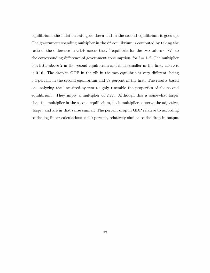
equilibrium, the in�ation rate goes down and in the second equilibrium it goes up.

The government spending multiplier in the ith equilibrium is computed by taking the

ratio of the di¤erence in GDP across the ith equilibria for the two values of Gl; to

the corresponding di¤erence of government consumption, for i = 1; 2: The multiplier

is a little above 2 in the second equilibrium and much smaller in the �rst, where it

is 0.16. The drop in GDP in the zlb in the two equilibria is very di¤erent, being

5.4 percent in the second equilibrium and 38 percent in the �rst. The results based

on analyzing the linearized system roughly resemble the properties of the second

equilibrium. They imply a multiplier of 2.77. Although this is somewhat larger

than the multiplier in the second equilibrium, both multipliers deserve the adjective,

�large�, and are in that sense similar. The percent drop in GDP relative to according

to the log-linear calculations is 6.0 percent, relatively similar to the drop in output

27

in the second equilibrium

Table 1: Properties of EW Equilibrium for Three Parameterizations

Panel A: Baseline parameterization

equilibrium #1 equilibrium #2 log-linear

dGDPdG

0.16 2.18 2.77

% drop in GDP 37.55 5.38 5.99

change in in�ation rate -11.77 -1.64 -1.90

eigenvalues in learning law of motion2:28; 1:4� 10�6;

1:9� 10�30:71;�2:5� 10�10;

�1:1� 10�4

� 0.0105

Panel B: Increase in p from 0.775 to 0.793 (longer expected duration of lower bound)dGDPdG

-2.84 5.36 12.41

% drop in GDP 25.49 13.21 38.60

change in in�ation rate -7.42 -3.85 -12.30

eigenvalues in learning law of motion1:27; -8.7� 10�7

�9:3� 10�50:85; 2:65� 10�10

�1:94� 10�4

� 0.00167

Panel C: Increase in � from 0.03 to 0.0375 (more �exibility in prices)dGDPdG

-2.08 4.54 414.3

% drop in GDP 25.44 12.20 1224.2

change in in�ation rate -8.22 -3.98 -444

eigenvalues in learning law of motion1:36; -9.3� 10�7

�1:7� 10�40:82; 1:3� 10�9

�2:8� 10�4

� 0.000056

We also compute the eigenvalues of the matrix, F; in (6.8). According to the

28

results in Table 1, the �rst equilibrium is not E-stable while the second one is.

We considered two perturbations on the baseline parameter values. Panel B

reports the results of increasing the expected duration of the zero lower bound by

raising the value of p from 0.775 to 0.793. The results are also reported in Figure 3.

Consistent with the implications of the linear approximation, the multiplier in the

second equilibrium is now increased. This matches one of the �ndings of CER, which

discusses the underlying intuition. However, note that the quantitative di¤erence

between the results based on linear approximation and the exact nonlinear analysis

is substantially larger. The multiplier implied by the linear approximation is now

a very large 12.4, more than twice its correct value of 5.36. Part of the reason the

multiplier jumped so much in the linear approximation, despite the tiny jump in

p; is that � in (5.9) falls by one order of magnitude from its value of 0.0105 in

the baseline parameterization, to 0.00167. In the �rst equilibrium, the government

spending multiplier falls somewhat with the rise in p; contradicting a basic conclusion

in CER that the multiplier and output drop in a binding zlb is more severe, the

greater is the expected duration of the zlb. However, Panel B indicates that, as

in Panel A, the �rst equilibrium in Figure 3 is not E-learnable, while the second is

E-learnable.

Next, consider Panel C which reports �ndings based on increasing "=�, i.e., mak-

ing prices more �exible (either by reducing adjustment costs or raising the elasticity

of demand). The result is that the slope of the Phillips curve rises from 0.03 in

the baseline parameterization to 0.0375. The results for this case are also displayed

in Figure 4. Based on the implications of the linear approximation, CER argued

that increased price �exibility increases the magnitude of the multiplier and of the

output collapse in the zlb. There is a simple intuition for this result, which is ex-

29

plained in CER.4 The second equilibrium con�rms the CER result: (i) the output

drop increases to roughly 12 percent, which is a little more than double its drop in

the baseline parameterization and (ii) the multiplier jumps from 2.18 in the baseline

model to 4.54 with more �exible prices. The linear approximation has qualitatively

the same implication, though the magnitudes are very di¤erent. In particular, ac-

cording to the linear approximation the output drop jumps from 5.99 percent in the

baseline parameterization to 1224 percent with more �exible prices. The multiplier

jumps from 2.77 in the baseline parameterization to 414 when prices are more �exi-

ble. That the e¤ects in the linear approximation are so very large re�ects that in this

example � is virtually zero, 0.000056. Further drops drive the multiplier and the

output drop to plus in�nity. Although the linear approximation is clearly far from

the mark quantitatively, its implications for the e¤ects of greater price �exibility are

qualitatively correct.

Note from the �rst equilibrium, however, that increased �exibility reduces the

multplier and the size of the output collapse in the zero lower bound, directly con-

tradicting the CER �nding. At the same time, Panel C indicates that the �rst

equilibrium is not E-stable.

To summarize, the basic qualitative results reported in CER using the log-linear

approximation holds up when we consider the nonlinear solution and ignore the �rst

equilibrium on the grounds of not being E-stable. In particular, (i) the government

spending multiplier can be considerably bigger than unity when the zlb binds, (ii)

as the expected duration of the zlb increases or the degree of �exibility of prices

increases, then both the severity of the output collapse in the zlb and the government

spending multiplier are larger, (iii) for parameterizations in which the output collapse

4For additional intuition, see Werning (2011).

30

is large, then the government spending multiplier is large too. The implications of the

linear approximation become increasingly distorted as parameter values are chosen

for which � approaches zero and turns negative. Although the properties of the

linear approximation change very sharply for ��s in this region, the properties of the

exact nonlinear solution are much less sensitive. However, we found that increases

in p and/or in " which have the e¤ect of reducing � eventually result in the non-

existence of equilibrium. This is because such parameter changes have the e¤ect of

shifting the f function down so that it does not intersect zero at any of the values

of �l considered. We discuss an example of this below.

7.2. Sunspot Equilibria

We consider sunspot equilibria simply by setting rl = rh = 1=� � 1 when evaluating

the f function. As before, the economy starts out in the �low�state and escapes with

constant probability, 1� p: In terms of Figure 2, we implement one change in the f

function, by setting rl = 1=� � 1: The resulting f functions (one each for the steady

state and high values of G) are exhibited in Figure 5.5 In terms of general shape and

number of crossings of the zero line, the f functions resemble the ones depicted in

Figures 2-4. In the present case, however, the second equilibrium is simply the steady

state equilibrium itself when G is constant and it is the steady state perturbed by

G in the case where G is temporarily high, in which the sunspot is ignored. In the

equilibrium #1 the sunspot has a non-trivial impact on prices and allocations, so we

call it the �sunspot equilibrium�.

As stressed in Mertens and Ravn (2011), the sunspot equilibrium can be charac-

terized as a situation in which the shock driving the economy into a binding zlb is a

5As in Figures 2-4, the higher curve corresponds to the case in which Gl = 1:05�Gh while the

sunspot shock is �low�and the lower curve corresponds to the case in which Gl = Gh:

31

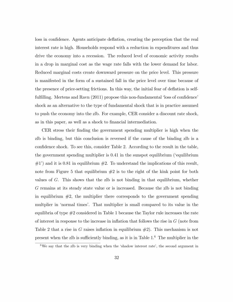
loss in con�dence. Agents anticipate de�ation, creating the perception that the real

interest rate is high. Households respond with a reduction in expenditures and thus

drive the economy into a recession. The reduced level of economic activity results

in a drop in marginal cost as the wage rate falls with the lower demand for labor.

Reduced marginal costs create downward pressure on the price level. This pressure

is manifested in the form of a sustained fall in the price level over time because of

the presence of price-setting frictions. In this way, the initial fear of de�ation is self-

ful�lling. Mertens and Ravn (2011) propose this non-fundamental �loss of con�dence�

shock as an alternative to the type of fundamental shock that is in practice assumed

to push the economy into the zlb. For example, CER consider a discount rate shock,

as in this paper, as well as a shock to �nancial intermediation.

CER stress their �nding the government spending multiplier is high when the

zlb is binding, but this conclusion is reversed if the cause of the binding zlb is a

con�dence shock. To see this, consider Table 2. According to the result in the table,

the government spending multiplier is 0.41 in the sunspot equilibrium (�equilibrium

#1�) and it is 0.81 in equilibrium #2. To understand the implications of this result,

note from Figure 5 that equilibrium #2 is to the right of the kink point for both

values of G. This shows that the zlb is not binding in that equilibrium, whether

G remains at its steady state value or is increased. Because the zlb is not binding

in equilibrium #2, the multiplier there corresponds to the government spending

multplier in �normal times�. That multiplier is small compared to its value in the

equilibria of type #2 considered in Table 1 because the Taylor rule increases the rate

of interest in response to the increase in in�ation that follows the rise in G (note from

Table 2 that a rise in G raises in�ation in equilibrium #2). This mechanism is not

present when the zlb is su¢ ciently binding, as it is in Table 1.6 The multiplier in the

6We say that the zlb is very binding when the �shadow interest rate�, the second argument in

32

sunspot equilibrium is essentially half of what it is in equilibrium #2. This suggests

that the CER conclusion is not robust to which shock drives the economy into a

binding zlb. We now examine other features of equilibrium #1 and #2, including

E-learnability.

According to the table, the percent drop inGDP whenG is expansionary, relative

to what GDP is in the high state, is a dramatic 43 percent (the GDP drop is a little

bigger in equilibrium #1 when G is held to its steady state value). This re�ects the

enormous size of the drop in anticipated in�ation (15 percent, at a quarterly rate!).

In the case of equilibrium #2, the drop in GDP is negative relative to steady state.

This re�ects that in the absence of an expansion in G; the second equilbrium simply

is the steady state equilibrium. So, the percent change in GDP in equilibrium #2

reported in Table 2 re�ects the positive impact of a rise in G on GDP . Similarly,

the rise in in�ation re�ects that an increase in G pushes the in�ation rate up. The

Taylor rule responds by raising the nominal rate of interest and this is what keeps

the multiplier small in equilibrium #2.

We considered the learnability of the equilibria in Figure 5. According to Table

2, one of the three eigenvalues of the matrix F in (6.8) associated with the sunspot

equilibrium exceeds unity. As a result, the equilibrium has the property that if agents

initially conjecture that aggregate quantities and prices deviate by a tiny amount

from their equilibrium values, the system will diverge from the sunspot equilibrium.

Moreover, the explosive eigenvalue is not just larger than unity, but it is enormous.

The system would propel itself away from the sunspot equilibrium at an extremely

the max operator in the policy rule, (2.5), is very negative. As a result, though the shadow interest

rate rises in response to the rise in G; it does not rise by enough to put the shadow interest rate

into the positive region. The outcome is that the actual interest rate remains constant after a rise

in G:

33

rapid rate. Equilibrium #2, on the other hand, is characterized by E-stability.

Table 2: Properties of Sunspot Equilibrium

Baseline parameters, except rl = 1=� � 1

equilibrium #1 equilibrium #2

dGDPdG

0.41 0.81

% drop in GDP 43.1 -0.81

change in in�ation rate -14.76 0.07

eigenvalues in learning law of motion3:82; 2:6� 10�6;

6:1� 10�30:83; 2:7� 10�11;

�8:8� 10�5

7.3. Absence of an Interior, EW Equilibrium

Expression (4.16) indicates that as p increases, for �l < 1, the f function shifts down.

Given the shape of that function in Figures 2, 3, 4, it is not surprising that for p

large enough, the function ceases to cross the zero line for �l 2 D, where D is de�ned

in (4.15). Indeed, when we adjust the baseline parameter values by setting p = 0:8;

this is what we �nd. There does not exist a �l 2 D for which f��l�= 0 (see Figure

6). In this case the model may have some other type of equilibrium, but it does not

have an interior, EW equilibrium. We found the same to be true when we change

parameters in a way that causes � to increase. To see this, note from (4.16) and

using (4.11), that real marginal cost, �hlC l; is less than unity when �l < 1: As a

result, increases in " drive the function, f; down for �l < 1: This is suggestive of our

numerical �nding that equilibrium ceases to exist as � increases.7

There is a loose connection between this absence of equilibrium and the extreme

behavior of the linearized economy as � converges to zero and then goes negative.

7These results are related to non-existence results obtained by Rhys Mendes (2011).

34

In our numerical experiments we found that equilibrium ceases to exist for values

of � or p that put � very slightly into the negative region. For example, in the

computation in Figure 6, � = �0:0016:

8. Deterministic Simulations

In practice, the framework described in the preceding sections is primarily used

to build intuition about the qualitative economic implications of the zlb. When

it is of interest to obtain quantitative results, researchers have typically turned to

deterministic simulations in which the shock that drives the economy into the zlb

is �on�for a known period of time.8 For example, CER use the EW framework to

build intuition about the dynamics of an economy in a binding zlb, but turn to

deterministic simulations of an estimated medium-sized DSGE model to investigate

the quantitative properties of an economy in a binding zlb. This section investigates

the quality of the linear approximation for these deterministic simulations. We do so

using the model of section 2, where the exact (and, unique) deterministic equilibrium

is easy to compute.9

We suppose that the economy begins in period t = 1 with a negative discount

rate, rt = rl. It is known that the discount rate will remain negative until t = T � 1

and that when t = T it switches permanently back to its steady state value of

1=� � 1: For the reasons explained in section 3, we assume that the system jumps

to its steady state in period T: To compute the equilibrium, we simulate the equilib-

rium conditions backwards, starting from steady state in period T: Since the model

8The wisdom of this strategy is supported by the recent analysis of Carlstrom, Fuerst and

Paustian (2012). They stress that the quantitative results based on the stochastic process for the

discount rate proposed by EW can be misleading.9Uniqueness re�ects in part our assumption about steady state in section 3.

35

has no initial conditions, this is a particularly straightforward strategy for �nding

the equilibrium.10 To see how we do this, rewrite the deterministic version of the

equilibrium conditions of the model, (2.2)-(2.6):

Ct =1 + rt

maxn1; 1

�+ � (�t � 1)

o�t+1Ct+1 (8.1)

ht = Ct +Gt +�

2(�t � 1)2 (Ct + Gt) (8.2)

(�t � 1)�t =1

�" (�Ctht � 1)

YtCt + Gt

+1

1 + rt(�t+1 � 1)�t+1

(Ct+1 + Gt+1)

Ct+1

CtCt + Gt

; (8.3)

for t = 0; 1; :::; T � 1: Here, Gt; rt are exogenous for t = 1; :::; T: This system of

equations induces a mapping from �t+1; Ct+1 to �t and Ct: We initiate the mapping

with �T and CT set to their steady state values. For given �t+1 and Ct+1 (8.1)-(8.3)

can be reduced to one equation in the one unknown, �t: For given �t; we use (8.1)

and (8.2) to compute Ct and ht; respectively: The in�ation rate, �t; is adjusted until

(8.3) is satis�ed using a numerical zero-�nding algorithm. An interior equilibrium

requires �t > 0. If gross in�ation were not positive, sign restrictions on the price level

and consumption (see (8.1)) would be violated: That each backward simulation step

requires �nding the zero of a nonlinear function draws attention to two possibilities:

(i) there may be no �t > 0 that solves the nonlinear equation for some t, in which

case there is no interior (i.e., where the e¢ ciency conditions hold with equality)

equilibrium and (ii) there may be multiple values of �t > 0 that solve the nonlinear

equation. To ensure that we do not miss (ii), we initiate the zero-�nding for each t

10When there is a given initial state, then this backward solution strategy requires back-

ward �shooting�, as in Christiano, Braggion and Roldos (2009). To see how this backward ap-

proach works in a stochastic setting when the equilibrium conditions have been linearized, see

http://faculty.wcas.northwestern.edu/~lchrist/course/Korea_2012/�xing_interest_rate.pdf

36

by �rst placing a �ne grid on a range of values of �t that extends from nearly zero

to 1.02. As before, we solve the model twice. The �rst time, we solve it for the case

where Gt is unchanged relative to its value in steady state. In the other case, Gt is

increased by 5 percent in each of periods t = 1; :::; T � 1: This second computation

allows us to deduce the government spending multiplier.

We now turn to the solution of the log-linearized system, (5.1)-(5.3). It is conve-

nient to express the Phillips curve in terms of yt; as in (5.4) (except, here p = 1):

yt =1� �g2� �g

1

�

��t � ��t+1 + �

�g1� �g

Gt

�: (8.4)

Conditional on �t+1; this represents a linear restriction across yt and �t: The IS curve

and policy rule (i.e., (5.1) and (5.3)) are:

yt � �gGt = yt+1 � �gGt+1 ��1� �g

�[� (Rt � 1� rt)� �t+1] (8.5)

Rt = max

�1;1

�+ � (�t � 1)

�; (8.6)

respectively. We solve (8.4)-(8.6) by applying the same backward simulation strategy

just described for (8.1)-(8.3). The calculations are initiated by setting �T = yT = 0:

At the tth step, we take �t+1 and yt+1 as given and compute �t and yt that solve

(8.4)-(8.6). We convert the problem of solving (8.4)-(8.6) into that of solving one

(nonlinear, because of (8.6)) equation in one unknown, �t: Given �t we use (8.4) to

solve for yt and (8.6) to solve for Rt: Finally, we adjust �t until (8.5) is satis�ed, if

this is possible.

We compute the government consumption multiplier at each date by (~yt � yt) =�~Gt �Gt

�;

where yt denotes GDP (� Ct +Gt) and a tilde over a variable indicates

Gt =

8<: 1:05�Gh t = 1; :::; T � 1

Gh t = T;

37

where Gh denotes the value of government consumption in steady state. Absence of

a tilde indicates that Gt = Gh for all t:

We found that for our baseline parameter values, there is a unique equilibrium for

the non-linear equilibrium conditions. As a result, we have a unique representation

of the level of GDP at each date. In the linear approximation, there are two locally

valid representations of the level of GDP; corresponding to two interpretations of yt

that are equivalent local to steady state:

yt =

8<:yt�yy

log (yt=y):

Here, y denotes the steady state value of yt:11 This gives rise to two ways of computing

the level of GDP :

yt =

8<: (yt + 1) y

y exp (yt):

Similarly, there are two representations of the government consumption multiplier:

dytdGt

=

8>><>>:eyt�yt

�g

heGt�Gt

iexp(eyt)�exp(yt)

�g

hexp

�eGt��exp(Gt)

i :

As before, a tilde signi�es the equilibrium in which government consumption is 5

percent above steady state for t = 1; :::; T �1 and absence of a tilde indicates govern-

ment spending is always at its steady state. Close to steady state, these two ways of

computing levels and the multiplier are equivalent. However, far from steady state

they are very di¤erent. For example, in the case of the exponential transformation,

11To see that these are equivalent, for yt close to y; note that under the �rst interpretation:

1 + yt =yty;

and that for yt small, log (1 + yt) ' yt:

38

yt is guaranteed to be non-negative, while in the case of the other transformation

non-negativity could be violated.

A numerical simulation is reported in Figure 7. We suppose that T = 22 and the

model parameters values are set at their baseline values, (7.1) (of course, p = 1 here).

In the �gure, the solid line represents the exact equilibrium, computed using the

nonlinear equations. The starred line represents the equilibrium approximated using

the linear approximation, with exponential transformation used to compute the level

of GDP (see �linear, exponential�). The line with circles indicates the e¤ects of

using the linear transformation on yt to compute the level of GDP (see �linear, non-

exponential�).

Consider the exact equilibrium �rst. Note that in the �rst period, output is

roughly 0.3, which is a substantial 70 percent below steady state. In that �rst period

there is a massive de�ation, amounting to -60 percent per quarter. The government

spending multiplier is 4 in the �rst period, and declines monotonically thereafter.

Although the shock driving the economy into the zlb does not lift until period 22;

the zlb ceases to bind in period 18. The �gure can be used to infer the equilibrium for

other values of T: For example, to see the equilibrium for T = 15; simply treat t = 8

as the �rst period. Similarly, for larger values of T; the initial period extrapolates

the results in the �gure to the left. From this it is not surprising that as T is

increased a little beyond T = 22; there ceases to exist a interior equilibrium.12 For

larger values of T; gross in�ation �wants�to go negative in the initial period. This

is not an interior equilibrium because it formally implies a negative price level and

negative consumption (see (8.1)). The fact that the output drop in the initial periods

is greater for larger values of T is another manifestation of the �nding in previous

12Recall, by interior equilibrium we mean one in which prices and quantities are non-zero and

e¢ ciency conditions hold with equality.

39

sections that the zlb is more severe for larger values of p: For the intuition behind

this result, see CER.

Consider now the performance of the linear-approximate solution. As one would

expect, when the system gets very far away from steady state, the accuracy of the

approximation deteriorates. From this perspective, it is very surprising that the

deterioration is negligible for in�ation and the interest rate. In terms of output and

the multiplier, the deterioration in performance is very severe for the non-exponential

transformation. For example, output is negative in periods 1 to 4. The multiplier

is over twice as large as its correct value in the �rst few periods. Interestingly,

approximation based on the exponential transformation of yt is quite good, even

very far away from steady state.

Figure 7 suggests that if we con�ne ourselves to the portion of the �gure where

output is within 20 percent of its steady state value (i.e., periods after t = 10); then

the approximation works very well, regardless of whether the linear or exponential

transformation of yt is used. For example, in the exact equilibrium, output is 0.81

in period t = 10; or 19 percent below steady state. According to the linear approxi-

mation, with non-exponential transformation on yt output is 0.77 in t = 0 and with

the exponential transformation on yt output is 0.80 in period t = 10: These errors in

approximation are small, particularly when we bear in mind that output is so very

far from steady state at t = 10. If we consider dates when output is closer to steady

state approximation error essentially vanishes. For example, in period t = 13 output

is 0.89, after rounding, in the exact equilibrium as well as in the two versions of the

linear approximation. As long as we use the exponential transformation on yt; the

approximation works well even when output is 50 or 60 percent away from its steady

state value. On the whole, Figure 7 provides substantial evidence in favor of the

accuracy of working with linear approximations.

40

9. Conclusion

We listed three conclusions reached by the literature on the zlb, obtained using lin-

earized equilibrium conditions. We �nd that these conclusions are robust to working

with non-linear equilibrium conditions and allowing for sunspot equilibria. Our �nd-

ing rests crucially on the use of E-learnability as an equilibrium selection device. The

plausibility of the E-learning criterion depends on the plausibility of the model of

learning used. We have explored one model of learning. A caveat to our analysis

is that there may be another model of learning that changes our results. We are

currently exploring other such approaches to learning.

41

References

[1] Benhabib, Jess, Stephanie Schmitt-Grohe and Martin Uribe, 2001, �Monetary

Policy and Multiple Equilibria�, American Economic Review 91, pp. 167�186.

[2] Braun, R. Anton, Lena Mareen Körber and Yuichiro Waki, 2012, �Some un-

pleasant properties of log-linearized solutions when the nominal rate is zero,�

February 15, unpublished manuscript, Federal Reserve Bank of Atlanta.

[3] Carlstrom, Charles T., Timothy S. Fuerst and Matthias Paustian, 2012, �A Note

on the Fiscal Multiplier Under an Interest Rate Peg,�February 16, manuscript,

Federal Reserve Bank of Cleveland.

[4] Christiano, Lawrence, Fabio Braggion and Jorge Roldos, 2009, �Optimal Mone-

tary Policy in a �Sudden Stop�, Journal of Monetary Economics 56, pp. 582-595.

[5] Christiano, Lawrence, Martin Eichenbaum and Sergio Rebelo, 2011, �When Is

the Government Spending Multiplier Large?,�Journal of Political Economy, Vol.

119, No. 1 (February), pp. 78-121.

[6] Christiano, Lawrence J., and Massimo Rostagno, 2001, �Money Growth Mon-

itoring and the Taylor Rule,�National Bureau of Economic Research Working

Paper 8539.

[7] Eggertson, Gauti B., 2011, �What Fiscal Policy is E¤ective at Zero Interest

Rates?�, 2010 NBER Macroconomics Annual 25, pp. 59�112.

[8] Eggertson, Gauti B. and Michael Woodford, 2003, �The Zero Bound on Interest

Rates and Optimal Monetary Policy�, Brookings Papers on Economic Activity

2003:1, pp. 139�211.

42

[9] Evans, G. W. and S. Honkapohja, 2001, Learning and Expectations in Macro-

economics, Princeton University Press.

[10] McCallum, Bennett T., 2007, �E-Stability vis-a-vis Determinacy Results for

a Broad Class of Linear Rational Expectations Models,�Journal of Economic

Dynamics and Control 31(4), April; 1376-1391.

[11] Mendes, Rhys, 2011, .

[12] Mertens, Karl and Morten O. Ravn, 2011, �Fiscal Policy in an Expectations

Driven Liquidity Trap,�July, manuscript, Cornell University.

[13] Rotemberg, Julio, 1982, Sticky Prices in the United States, Journal of Political

Economy, Vol. 90, No. 6 (December), pp. 1187-1211.

[14] Werning, Ivan, 2011, �Managing a Liquidity Trap: Monetary and Fiscal Policy,�

unpublished manuscript, Massachusetts Institute of Technology.

43

Figure 1: BSGU Demonstration of Two Steady States

R

π

Fisher equation,slope = 1/β

Taylor rule, slope = α

1

Two steady states:

β 1

0.88 0.9 0.92 0.94 0.96 0.98 1-2

-1.5

-1

-0.5

0

0.5

1

1.5

2

2.5

3

x 10-3

l

cap-delta = 0.010519 kap = 0.03 eps = 3, bet = 0.99, alph = 1.5, p = 0.775, rl = -0.005, phi = 100, eps/phi = 0.03 psi = 1 etag = 0.2 Gl/Gh = 1.05, multiplier in 1st equil = 0.15936, in 2nd equil = 2.1761 1st equilibrium, inflation = -11.7738, consumption = 0.41449, employment = 1.0573, GDP = 0.62449 adjustment costs/GDP = 0.69311, Z = 0.83349 percent drop in GDP = 37.5506 2nd equilibrium, inflation = -1.6433, consumption = 0.73618, employment = 0.95896, GDP = 0.94618 adjustment costs/GDP = 0.013503, Z = 0.98545 percent drop in GDP = 5.3817

implications of linear approximation: percent drop in output = 5.9941, inflation rate = -1.8995, multiplier = 2.7683

Gl>Gh

Gl=Gh

Zero bound ceases to bind at πl = 0.9933

Equilibrium #1 Equilibrium #2

Figure 2: EW EquilibriaInterval of candidate EW equilibrium inflation rates: [0.78,2.27]. There are no other zeros.

f l

Rise in G makes inflation risein lower equilibrium and fallin higher equilibrium.

Figure 3: Longer Expected Duration

0.88 0.9 0.92 0.94 0.96 0.98 1-20

-15

-10

-5

0

x 10-4

l

cap-delta = 0.0016685 kap = 0.03 eps = 3, bet = 0.99, alph = 1.5, p = 0.793, rl = -0.005, phi = 100, eps/phi = 0.03 psi = 1 etag = 0.2 Gl/Gh = 1.05, multiplier in 1st equil = -2.8396, in 2nd equil = 5.3588 1st equilibrium, inflation = -7.4189, consumption = 0.53509, employment = 0.95013, GDP = 0.74509 adjustment costs/GDP = 0.2752, Z = 0.89882 percent drop in GDP = 25.4912

2nd equilibrium, inflation = -3.8523, consumption = 0.65788, employment = 0.93228, GDP = 0.86788 adjustment costs/GDP = 0.074199, Z = 0.95232 percent drop in GDP = 13.2115 implications of linear approximation: percent drop in output = 38.6044, inflation rate = -12.2984, multiplier = 12.4066

Gl>Gh

Gl=Ghf l

Similar picture to previous one.Note that increase in p reduceslevel of curves…..moves Δ downand increases chance of no equilibrium.

Figure 4: More Flexible Prices

0.88 0.9 0.92 0.94 0.96 0.98 1-20

-15

-10

-5

0

5x 10

-4

l

cap-delta = 5.625e-005 kap = 0.0375 eps = 3.75, bet = 0.99, alph = 1.5, p = 0.775, rl = -0.005, phi = 100, eps/phi = 0.0375 psi = 1 etag = 0.2 Gl/Gh = 1.05, multiplier in 1st equil = -2.0843, in 2nd equil = 4.5438 1st equilibrium, inflation = -8.2161, consumption = 0.53556, employment = 0.9972, GDP = 0.74556 adjustment costs/GDP = 0.33752, Z = 0.88686 percent drop in GDP = 25.4443

2nd equilibrium, inflation = -3.9804, consumption = 0.66799, employment = 0.94755, GDP = 0.87799 adjustment costs/GDP = 0.079216, Z = 0.9504 percent drop in GDP = 12.2005 implications of linear approximation: percent drop in output = 1224.2267, inflation rate = -444, multiplier = 414.3333

Gl>Gh

Gl=Ghf l

Increased price flexibility raises κ and, hence, Δ. Also,increases chance of no equilibriumby pushing curves down.

0.84 0.86 0.88 0.9 0.92 0.94 0.96 0.98 1 1.02-2

0

2

4

6

8

x 10-3

l

cap-delta = 0.010519 kap = 0.03 eps = 3, bet = 0.99, alph = 1.5, p = 0.775, rl = 0.010101, phi = 100, eps/phi = 0.03 psi = 1 etag = 0.2 Gl/Gh = 1.05, multiplier in 1st equil = 0.41074, in 2nd equil = 0.81222 1st equilibrium, inflation = -14.7618, consumption = 0.3587, employment = 1.1883, GDP = 0.5687 adjustment costs/GDP = 1.0896, Z = 0.78867 percent drop in GDP = 43.1301

2nd equilibrium, inflation = 0.074496, consumption = 0.79812, employment = 1.0082, GDP = 1.0081 adjustment costs/GDP = 2.7748e-005, Z = 1.0112 percent drop in GDP = -0.81222

Gl > Gh

Gl = Gh

Figure 5: Sunspot Equilibrium

Equilibrium in which the model does not respond to sunspot.

Sunspot equilibrium (Mertens‐Ravn)

f l

Figure 6: No Equilibrium

0.9 1 1.1 1.2 1.3 1.4 1.5 1.6 1.7 1.8 1.9-0.1

-0.08

-0.06

-0.04

-0.02

0

0.02

cap-delta = -0.0016 kap = 0.03 eps = 3, bet = 0.99, alph = 1.5, p = 0.8, rl = -0.005, phi = 100, eps/phi = 0.03 psi = 1 etag = 0.2 Gl/Gh = 1

l

f l

Figure 7: Deterministic Simulation

2 4 6 8 10 12 14 16 18 20 22

0.4

0.5

0.6

0.7

0.8

0.9

1gross inflation

2 4 6 8 10 12 14 16 18 20 220.995

1

1.005

1.01gross nominal rate (R)

2 4 6 8 10 12 14 16 18 20 22

-0.6

-0.4

-0.2

0

0.2

0.4

0.6

0.8

1GDP

2 4 6 8 10 12 14 16 18 20 22

2

4

6

8

10

12

14government consumption multiplier

nonlinearlinear, exponentiallinear, non-exponential