Solution Manual07
94
CHAPTER 7 Activity Analysis, Cost Behavior, and Cost Estimation ANSWERS TO REVIEW QUESTIONS 7-1 Cost behavior patterns are important in the process of making cost predictions. Cost predictions are used in planning, control, and decision making. For example, cost budgets are based on predictions of costs at various levels of activity. Cost control is accomplished by comparing actual costs against budgeted costs, which are based on cost predictions. Cost predictions are also important in decision making, since the desirability of various alternatives often depends on the costs that will be incurred under those alternatives. 7-2 a. Cost estimation is the process of determining how a particular cost behaves. b. Cost behavior is the relationship between cost and activity. c.Cost prediction is the forecast of cost at a particular level of activity. Cost estimation determines the cost behavior pattern, which is used to make a cost prediction about the cost at a particular level of activity contemplated in the future. 7-3 a. Hotel: Percentage of rooms occupied or the number of occupancy-days, where an occupancy-day is defined as one room occupied for one day. McGraw-Hill/Irwin 2002 The McGraw-Hill Companies, Inc. Managerial Accounting, 5/e 7-1
-
Upload
ganesh-shankar -
Category
Documents
-
view
106 -
download
2
description
solution
Transcript of Solution Manual07

CHAPTER 7Activity Analysis, Cost Behavior, and Cost Estimation
ANSWERS TO REVIEW QUESTIONS
7-1 Cost behavior patterns are important in the process of making cost predictions. Cost predictions are used in planning, control, and decision making. For example, cost budgets are based on predictions of costs at various levels of activity. Cost control is accomplished by comparing actual costs against budgeted costs, which are based on cost predictions. Cost predictions are also important in decision making, since the desirability of various alternatives often depends on the costs that will be incurred under those alternatives.
7-2 a. Cost estimation is the process of determining how a particular cost behaves.
b. Cost behavior is the relationship between cost and activity.
c. Cost prediction is the forecast of cost at a particular level of activity.
Cost estimation determines the cost behavior pattern, which is used to make a cost prediction about the cost at a particular level of activity contemplated in the future.
7-3 a. Hotel: Percentage of rooms occupied or the number of occupancy-days, where an occupancy-day is defined as one room occupied for one day.
b. Hospital: Patient-days, where a patient-day is defined as a one-day stay by one patient.
c. Computer manufacturer: Number of computers manufactured, throughput, engineering specifications, engineering change orders, or number of parts in the finished product.
d. Computer sales store: Sales revenue.
e. Computer repair service: Repair calls or hours of repair service.
f. Public accounting firm: Hours of auditing service provided by each classification of personnel (partner, manager, supervisor, senior accountant, and staff accountant).
McGraw-Hill/Irwin 2002 The McGraw-Hill Companies, Inc.Managerial Accounting, 5/e 7-1
7-4 Graphs of the cost behavior patterns are as follows:
McGraw-Hill/Irwin 2002 The McGraw-Hill Companies, Inc.7-2 Solutions Manual
Cost Cost
Activity Activity
Cost Cost
Activity Activity
Cost Cost
Activity Activitya. Variable b. Step-variable
c. Fixed d. Step-fixed
e. Semivariable f. Curvilinear
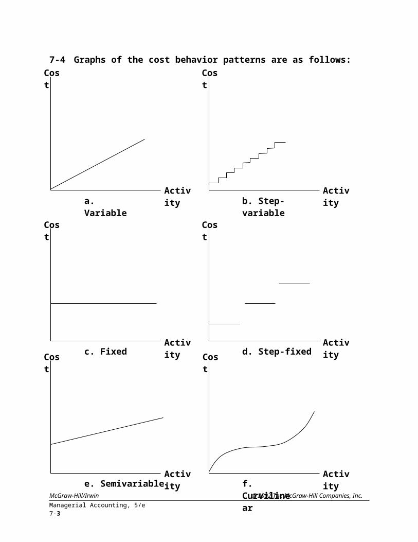
7-5 As the level of activity (or cost driver) increases, total fixed cost remains constant. However, the fixed cost per unit of activity declines as activity increases.
7-6 A manufacturer's cost of supervising production might be a step-fixed cost, because one supervisor is needed for each shift. Each shift can accommodate a certain range of production activity; when activity exceeds that range, a new shift must be added. When the new shift is added, a new production supervisor must be employed. This new position results in a jump in the step-fixed cost to a higher level.
7-7 As the level of activity (or cost driver) increases, total variable cost increases proportionately and the variable cost per unit remains constant.
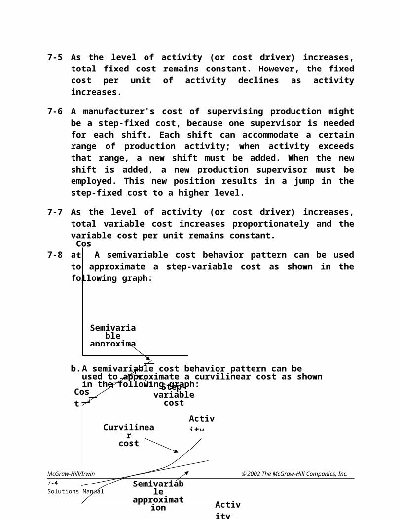
7-8 a. A semivariable cost behavior pattern can be used to approximate a step-variable cost as shown in the following graph:
McGraw-Hill/Irwin 2002 The McGraw-Hill Companies, Inc.Managerial Accounting, 5/e 7-3
Activity
Semivariableapproximation
Step-variablecost
A semivariable cost behavior pattern can be used to approximate a curvilinear cost as shown in the following graph:
Cost
Cost
Activity
Curvilinearcost
Semivariableapproximation
b.
7-9 (a) Annual cost of maintaining an interstate highway: committed cost. (Once the highway has been built, it must be maintained. The transportation authorities are largely committed to spending the necessary funds to maintain the highway adequately.)
(b) Ingredients in a breakfast cereal: engineered cost.
(c) Advertising for a credit card company: discretionary cost.
(d) Depreciation on an insurance company's computer: committed cost.
(e) Charitable donations: discretionary cost.
(f) Research and development: discretionary cost.
7-10 The cost analyst should respond by pointing out that in most cases a cost behavior pattern should be limited to the relevant range of activity. When the firm's utility cost was shown as a semivariable cost, it is likely that only some portion in the middle of the graph would fall within the relevant range. Within the relevant range, the firm's utility cost can be approximated reasonably closely by a semivariable cost behavior pattern. However, outside that range (including an activity level of zero), the semivariable cost behavior pattern should not be used as an approximation of the utility cost.
7-11 A learning curve shows how average labor time per unit of production changes as cumulative output changes. In many production processes, as production activity increases and learning takes place, there is a significant reduction in the amount of labor time required per unit. The learning phenomenon is important in cost estimation, since estimates must often be made for the level of cost to be incurred after additional production experience is gained.
7-12 Work measurement is the systematic analysis of a task for the purpose of determining the inputs needed to perform the task. Work measurement is sometimes used to help in estimating the costs of various nonmanufacturing activities. The unit of analysis in work measurement often is called a control factor unit. Appropriate control factor units for several tasks are as follows:
a. Handling materials at a loading dock: Weight of materials handled.
b. Registering vehicles at a county motor vehicle office: Number of registrations processed.
McGraw-Hill/Irwin 2002 The McGraw-Hill Companies, Inc.7-4 Solutions Manual
c. Picking oranges: Volume or weight of oranges picked.
d. Inspecting computer components in an electronics firm: Number of components inspected.
7-13 An outlier is a data point that falls far away from the other points in the scatter diagram and is not representative of the data. One possible cause of an outlier is simply a mistake in recording the data. Another cause of an outlier is a random event that occurred, which caused the cost during a particular period to be unusually high or low. For example, a power outage may have resulted in unusually high costs of idle time for a particular time period. Outliers should be eliminated from a data set upon which cost estimates are based.
7-14 Fixed costs are often allocated on a per unit-of-activity basis. For example, fixed manufacturing-overhead costs, such as depreciation, may be allocated to units of production. As a result, such costs may appear to be variable in the cost records. Discretionary costs often are budgeted in a manner that makes them appear variable. A cost such as charitable donations, for example, may be fixed once management decides on the level of donations to be made. If management's policy is to budget charitable donations on the basis of sales dollars, however, the cost will appear to be variable to the cost analyst. An experienced analyst should be wary of allocated and discretionary costs and take steps to learn how the amounts are determined.
7-15 In the first step of the visual-fit method of cost estimation, data points are plotted on graph paper to form a scatter diagram. Then a line is drawn through the scatter diagram in an attempt to minimize the distance between the line and the plotted points. The scatter diagram and the visually-fitted cost line provide a valuable first approximation in the analysis of any cost suspected to be semivariable or curvilinear. The method is easy to use and to explain to others and provides a useful view of the overall cost behavior pattern. The visual-fit method also enables an experienced cost analyst to spot outliers in the data. The primary drawbacks of the visual-fit method are its lack of objectivity. Two cost analysts may draw two different visually-fitted cost lines.
7-16 The chief drawback of the high-low method of cost estimation is that it uses only two data points. The rest of the data are ignored by the method. An outlier can cause a significant problem when the high-low method is used if one of the two data points happens to be an outlier. In other words, if the high activity level happens to be associated with a cost that is not representative of the data, the resulting cost line may not be representative of the cost behavior pattern.
McGraw-Hill/Irwin 2002 The McGraw-Hill Companies, Inc.Managerial Accounting, 5/e 7-5
7-17 The term least squares in the least-squares regression method of cost estimation refers to the process of minimizing the sum of the squares of the distances between the data and the regression line.
7-18 A least-squares regression line may be expressed in equation form as follows:
Y = a + bX
In this equation, X is referred to as the independent variable, since it is the variable upon which the estimate is based. Y is called the dependent variable, since its estimate depends on the independent variable. The intercept of the line on the vertical axis is denoted by a, and the slope of the line is denoted by b. Within the relevant range, a is interpreted as an estimate of the fixed-cost component, and b is interpreted as an estimate of the variable cost per unit of activity.
7-19 In simple regression there is a single independent variable. In multiple regression there are two or more independent variables.
7-20 Advanced manufacturing technology, such as FMS and CIM systems, have resulted in a shift in the cost structure toward fixed costs. Moreover, many of these fixed costs are committed costs.
7-21 A particular least-squares regression line may be evaluated on the basis of economic plausibility or goodness of fit.
The cost analyst should always evaluate a regression line from the perspective of economic plausibility. Does the regression line make economic sense? Is it intuitively plausible? An experienced cost analyst should have a good feel for whether the regression line looks reasonable.
Statistical methods can also be used to determine how well a regression line fits the data upon which it is based. This method is referred to as assessing the goodness of fit of the regression. A commonly used measure of goodness of fit is the coefficient of determination, which is described in the appendix at the end of the chapter. The coefficient of determination is also denoted by R2.
McGraw-Hill/Irwin 2002 The McGraw-Hill Companies, Inc.7-6 Solutions Manual
SOLUTIONS TO EXERCISES
EXERCISE 7-22 (40 MINUTES)
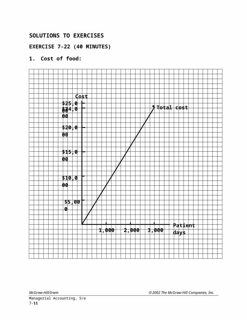
1. Cost of food:
McGraw-Hill/Irwin 2002 The McGraw-Hill Companies, Inc.Managerial Accounting, 5/e 7-7
Cost$25,000$24,000
$20,000
$15,000
$10,000
$5,000
1,000 2,000 3,000Patient days
Total cost
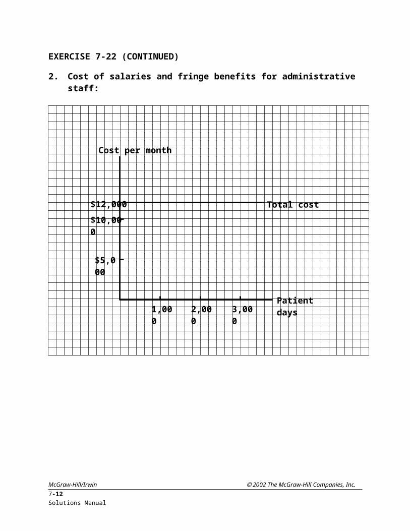
EXERCISE 7-22 (CONTINUED)
2. Cost of salaries and fringe benefits for administrative staff:
McGraw-Hill/Irwin 2002 The McGraw-Hill Companies, Inc.7-8 Solutions Manual
Patient days1,000 2,000 3,000
$12,000
$10,000
$5,000
Total cost
Cost per month
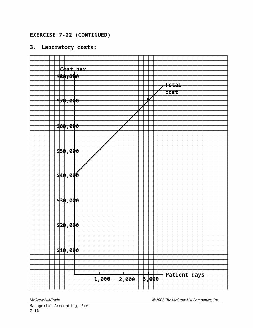
EXERCISE 7-22 (CONTINUED)
3. Laboratory costs:
McGraw-Hill/Irwin 2002 The McGraw-Hill Companies, Inc.Managerial Accounting, 5/e 7-9
Total cost
Cost per month$80,000
$70,000
$60,000
$50,000
$40,000
$30,000
$20,000
$10,000
1,000 2,000 3,000Patient days

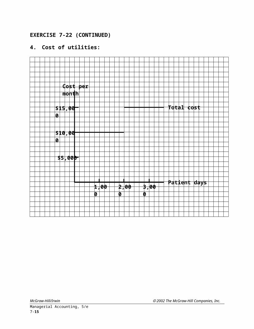
EXERCISE 7-22 (CONTINUED)
4. Cost of utilities:
McGraw-Hill/Irwin 2002 The McGraw-Hill Companies, Inc.7-10 Solutions Manual
Total cost
Patient days1,000 2,000 3,000
$15,000
$10,000
$5,000
Cost per month
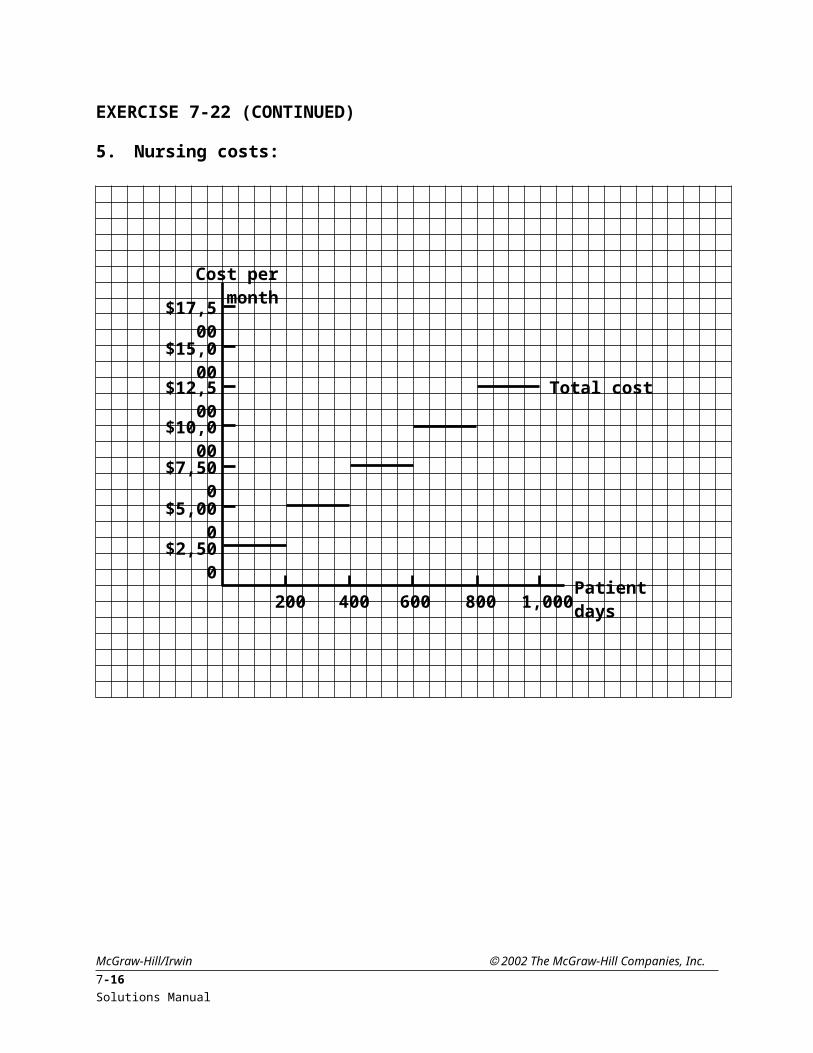
EXERCISE 7-22 (CONTINUED)
5. Nursing costs:
McGraw-Hill/Irwin 2002 The McGraw-Hill Companies, Inc.Managerial Accounting, 5/e 7-11
Total cost
Patient days200 400 600 800 1,000
$15,000
$12,500
$10,000
$7,500
$5,000
$2,500
Cost per month
$17,500
EXERCISE 7-23 (15 MINUTES)
1.Actual Estimated
a. 20,000 miles................................................................... $3,900 $4,400b. 40,000 miles................................................................... 5,200 5,200c. 60,000 miles................................................................... 6,000 6,000d. 90,000 miles................................................................... 8,500 7,200
2. (a) The approximation is very accurate in the range 40,000 to 60,000 miles per month.
(b) The approximation is less accurate in the extremes of the longer range, 20,000 to 90,000 miles.
EXERCISE 7-24 (15 MINUTES)
1.Cost per Broadcast Hour
Cost Item July SeptemberProduction crew:
$4,875/390 hr............................................. $12.50 per hr.$8,000/640 hr............................................. $12.50 per hr.
Supervisory employees:$5,000/390 hr............................................. 12.82 per hr.*$5,000/640 hr............................................. 7.81 per hr.*
*Rounded.
2. December cost predictions:
Production crew (420 $12.50 per hr.)............................................. $5,250Supervisory employees....................................................................... 5,000
3.
Cost ItemCost per Broadcast Hour
in DecemberProduction crew......................................................... $12.50 per hr.
Supervisory employees ($5,000/420 hr.).................. 11.90 per hr.*
*Rounded.EXERCISE 7-25 (15 MINUTES)
1.Variable cost per pint of applesauce produced =
McGraw-Hill/Irwin 2002 The McGraw-Hill Companies, Inc.7-12 Solutions Manual
Total cost at 41,000 pints............................................................................ $24,100Variable cost at 41,000 pints
(41,000 $.10 per pint)..................................................................... 4,100Fixed cost...................................................................................................... $20,000
Cost equation:
Total energy cost = $20,000 + $.10X, where X denotes pints of applesauce produced
2. Cost prediction when 26,000 pints of applesauce are produced
Energy cost = $20,000 + ($.10)(26,000) = $22,600
McGraw-Hill/Irwin 2002 The McGraw-Hill Companies, Inc.Managerial Accounting, 5/e 7-13

EXERCISE 7-26 (30 MINUTES)
1. Scatter diagram and visually-fitted line:
McGraw-Hill/Irwin 2002 The McGraw-Hill Companies, Inc.7-14 Solutions Manual
Monthly energy cost
$30,000
$25,000
$20,000
$15,000
$10,000
$5,000
10,000 20,000 30,000 40,000 50,000Pints of apple
sauce produced
EXERCISE 7-26 (CONTINUED)
2. Answers will vary on this requirement because of variation in the visually-fitted lines.
Based on the preceding plot, the cost prediction at 26,000 pounds is:
Energy cost = $22,600
3. The July cost observation at the 40,000-pint activity level appears to be an outlier. The cost analyst should check the observation data for accuracy. If the data are accurate, the outlier should be ignored in making cost predictions.
EXERCISE 7-27 (30 MINUTES)
Answers will vary widely, depending on the company and costs selected. Some examples of typical manufacturing costs follow.
Direct material: variable
Electricity: variable
Depreciation on plant and equipment: fixed
Plant manager’s salary: fixed
Property taxes: fixed
McGraw-Hill/Irwin 2002 The McGraw-Hill Companies, Inc.Managerial Accounting, 5/e 7-15
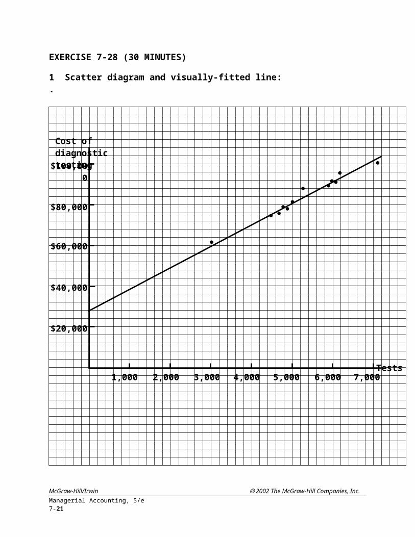
EXERCISE 7-28 (30 MINUTES)
1. Scatter diagram and visually-fitted line:
McGraw-Hill/Irwin 2002 The McGraw-Hill Companies, Inc.7-16 Solutions Manual
Cost of diagnostic testing
$100,000
$80,000
$60,000
$40,000
$20,000
1,000 7,000Tests
6,0005,0002,000 3,000 4,000

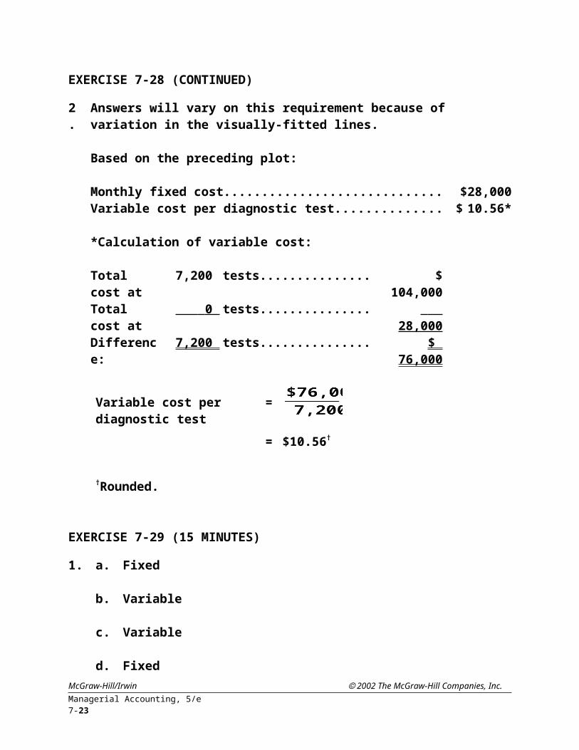
EXERCISE 7-28 (CONTINUED)
2. Answers will vary on this requirement because of variation in the visually-fitted lines.
Based on the preceding plot:
Monthly fixed cost.............................................................................................. $28,000Variable cost per diagnostic test...................................................................... $ 10.56*
*Calculation of variable cost:
Total cost at 7,200 tests............................................ $ 104,000Total cost at 0 tests............................................ 28,000 Difference: 7,200 tests............................................ $ 76,000
Variable cost per diagnostic test =
= $10.56†
†Rounded.
EXERCISE 7-29 (15 MINUTES)
1. a. Fixed
b. Variable
c. Variable
d. Fixed
e. Semivariable (or mixed)
2. Production cost per month = $33,000* + $2.00X †
*33,000 = $19,000 + $10,000 + $4,000†$2.00 = $1.10 + $.70 + $.20
McGraw-Hill/Irwin 2002 The McGraw-Hill Companies, Inc.Managerial Accounting, 5/e 7-17

EXERCISE 7-30 (15 MINUTES)
1. Variable maintenance
cost per tour mile = (12,500r-11,000r) / (20,000 miles – 8,000 miles)
= .125r
r denotes the real, Brazil’s national currency.
Total maintenance cost at 8,000 miles........................................................ 11,000rVariable maintenance cost at 8,000 miles (.125r 8,000)........................ 1,000 r Fixed maintenance cost per month............................................................. 10,000 r
2. Cost formula:
Total maintenance cost per month = 10,000r + .125rX , where X denotes tour miles traveled during the month.
3. Cost prediction at the 22,000-mile activity level:
Maintenance cost = 10,000r + (.125r)(22,000)
= 12,750r
McGraw-Hill/Irwin 2002 The McGraw-Hill Companies, Inc.7-18 Solutions Manual

EXERCISE 7-31 (15 MINUTES)
McGraw-Hill/Irwin 2002 The McGraw-Hill Companies, Inc.Managerial Accounting, 5/e 7-19
Total cost when 100 audits are performedin a month: $78,200 = $10,000 + ($682) (100)
Monthly audit cost
$100,000
$80,000
$60,000
$40,000
$20,000
20 40 60 80 100
Control factor units: tax returns audited
Fixed cost per month: $10,000

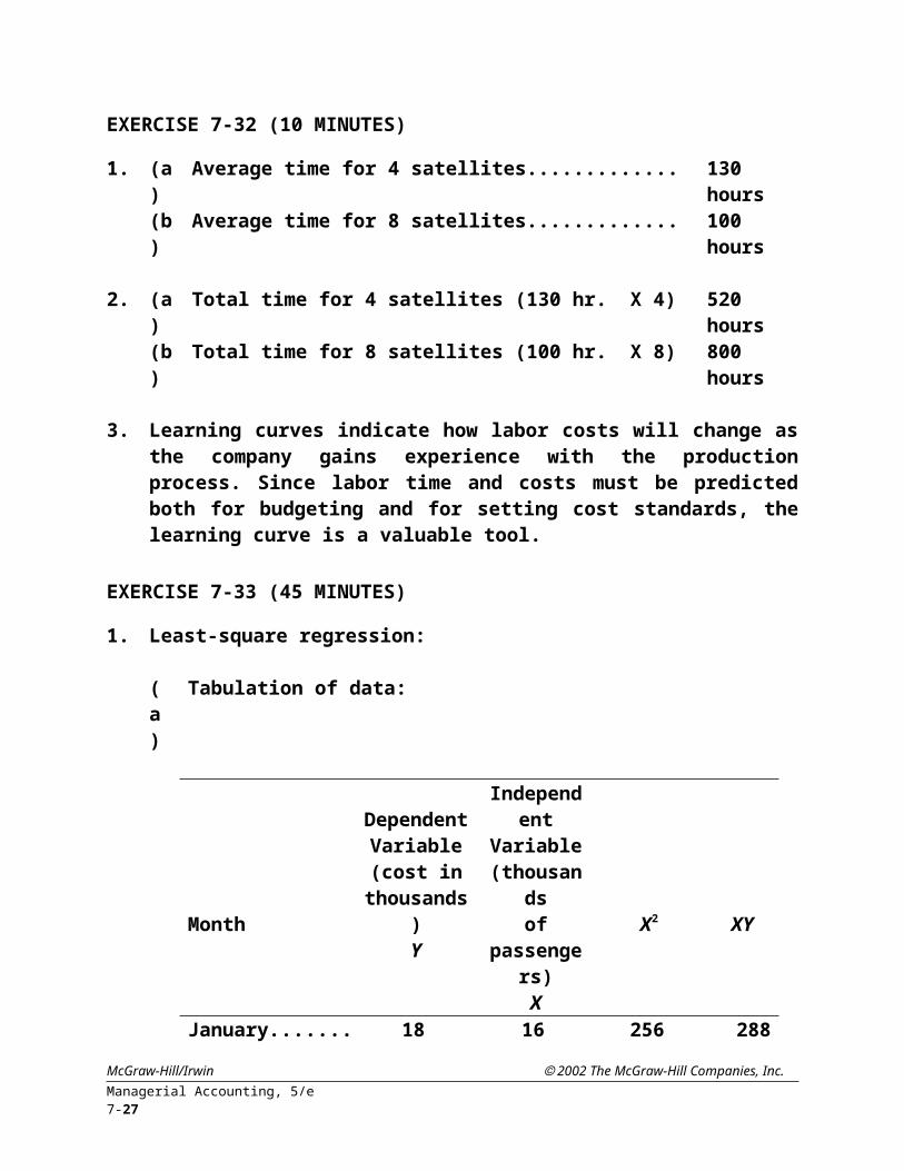
EXERCISE 7-32 (10 MINUTES)
1. (a) Average time for 4 satellites............................................................... 130 hours(b) Average time for 8 satellites............................................................... 100 hours
2. (a) Total time for 4 satellites (130 hr. X 4).............................................. 520 hours(b) Total time for 8 satellites (100 hr. X 8).............................................. 800 hours
3. Learning curves indicate how labor costs will change as the company gains experience with the production process. Since labor time and costs must be predicted both for budgeting and for setting cost standards, the learning curve is a valuable tool.
EXERCISE 7-33 (45 MINUTES)
1. Least-square regression:
(a) Tabulation of data:
Month
Dependent Variable (cost in
thousands)Y
Independent Variable
(thousandsof
passengers)X X2 XY
January....................... 18 16 256 288February...................... 18 17 289 306March........................... 19 16 256 304April............................. 20 18 324 360May.............................. 18 15 225 270June............................. 19 17 289 323 Total............................. 112 99 1,639 1,851
McGraw-Hill/Irwin 2002 The McGraw-Hill Companies, Inc.7-20 Solutions Manual
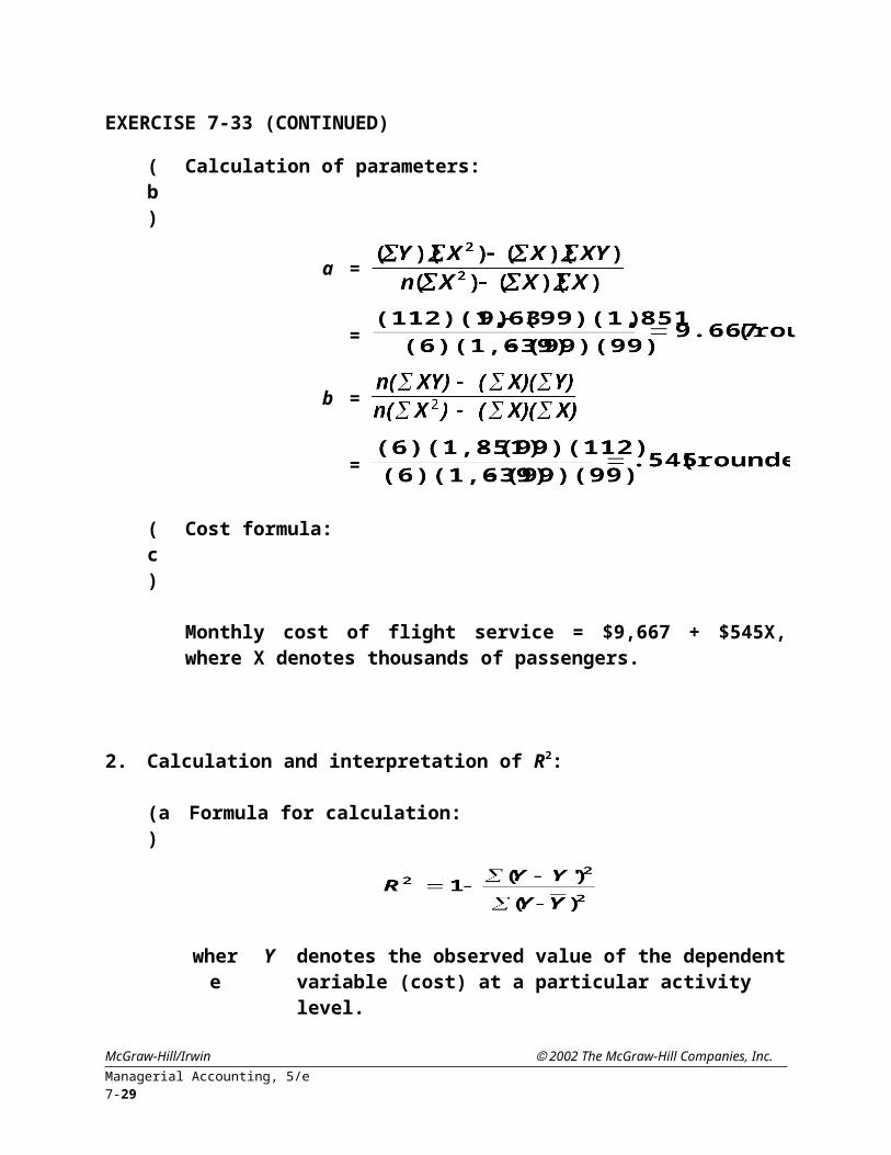
EXERCISE 7-33 (CONTINUED)
(b) Calculation of parameters:
a =
=
b =
=
(c) Cost formula:
Monthly cost of flight service = $9,667 + $545X, where X denotes thousands of passengers.
2. Calculation and interpretation of R2:
(a) Formula for calculation:
where Y denotes the observed value of the dependent variable (cost) at a particular activity level.
Y' denotes the predicted value of the dependent variable (cost) based on the regression line, at a particular activity level.
denotes the mean (average) observation of the dependent variable (cost).
McGraw-Hill/Irwin 2002 The McGraw-Hill Companies, Inc.Managerial Accounting, 5/e 7-21

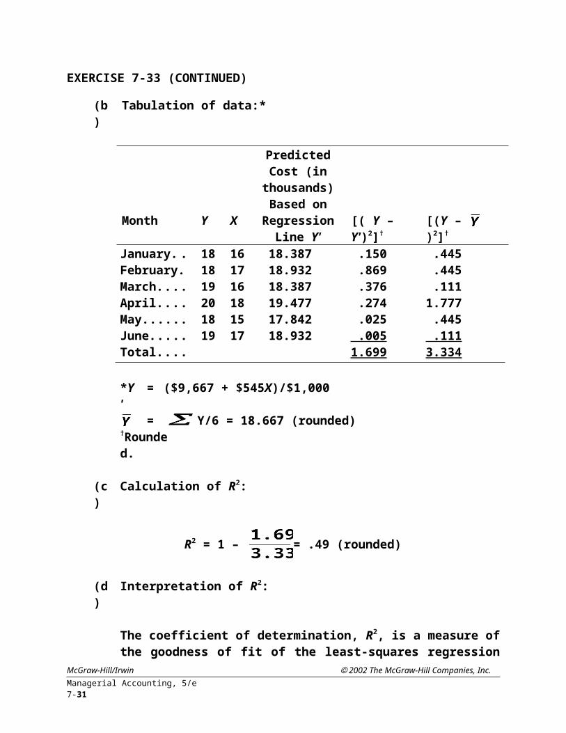
EXERCISE 7-33 (CONTINUED)
(b) Tabulation of data:*
Month Y X
Predicted Cost (in thousands)Based on
RegressionLine Y' [( Y – Y')2]† [(Y – )2]†
January.......... 18 16 18.387 .150 .445February......... 18 17 18.932 .869 .445March.............. 19 16 18.387 .376 .111April................ 20 18 19.477 .274 1.777May................. 18 15 17.842 .025 .445June................ 19 17 18.932 .005 .111Total................ 1.699 3.334
*Y' = ($9,667 + $545X)/$1,000= Y/6 = 18.667 (rounded)
†Rounded.
(c) Calculation of R2:
R2 = 1 – = .49 (rounded)
(d) Interpretation of R2:
The coefficient of determination, R2, is a measure of the goodness of fit of the least-squares regression line. An R2 of .49 means that 49% of the variability of the dependent variable about its mean is explained by the variability of the independent variable about its mean. The higher the R2, the better the regression line fits the data. The interpretation of a high R2 is that the independent variable is a good predictor of the behavior of the dependent variable. In cost estimation, a high R2 means that the cost analyst can be relatively confident in the cost predictions based on the estimated-cost behavior pattern.
McGraw-Hill/Irwin 2002 The McGraw-Hill Companies, Inc.7-22 Solutions Manual
EXERCISE 7-34 (45 MINUTES)
1. Variable utility cost per hour = = $2.00
Total utility cost at 700 hours....................................................................... $ 1,900Variable utility cost at 700 hours ($2.00 700 hours).............................. 1,400 Fixed cost per month.................................................................................... $ 500
Cost formula:
Monthly utility cost = $500 + $2.00 X , where X denotes hours of operation.
2. Variable-cost estimate based on the scatter diagram on the next page:
Cost at 600 hours ........................................................................ $1,700Cost at 0 hours ........................................................................ 450Difference 600 hours ........................................................................ $1,250
Variable cost per hour = $1,250/600 hr. = $2.08 (rounded)
McGraw-Hill/Irwin 2002 The McGraw-Hill Companies, Inc.Managerial Accounting, 5/e 7-23

EXERCISE 7-34 (CONTINUED)
Scatter diagram and visually-fitted line:
McGraw-Hill/Irwin 2002 The McGraw-Hill Companies, Inc.7-24 Solutions Manual
Utility costper month
$2,500
$2,000
$1,500
$1,000
$500
100 200 300 400 500 600 700Hours ofoperation

EXERCISE 7-34 (CONTINUED)
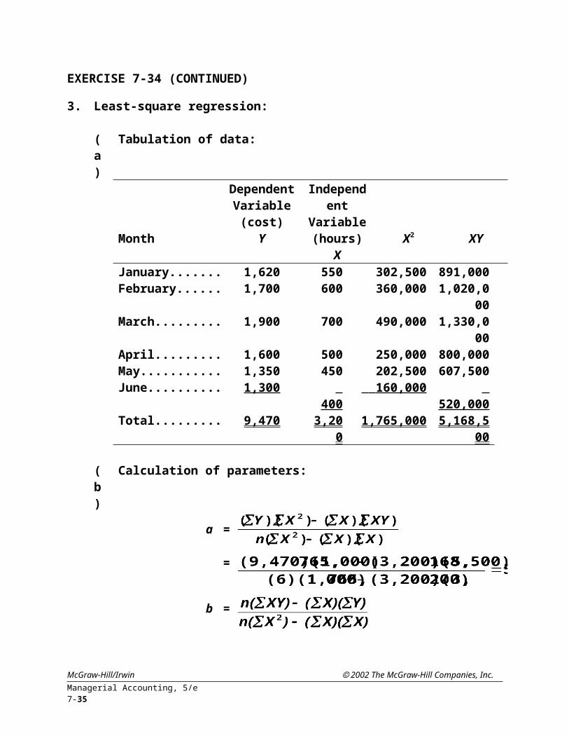
3. Least-square regression:
(a) Tabulation of data:
Month
Dependent Variable
(cost)Y
Independent Variable (hours)
X X2 XYJanuary....................... 1,620 550 302,500 891,000February...................... 1,700 600 360,000 1,020,000March........................... 1,900 700 490,000 1,330,000April............................. 1,600 500 250,000 800,000May.............................. 1,350 450 202,500 607,500June............................. 1,300 400 160,000 520,000 Total............................. 9,470 3,200 1,765,000 5,168,500
(b) Calculation of parameters:
a =
=
b =
=
(c) Cost formula:
Monthly utility cost = $501 + $2.02X, where X denotes hours of operation.
Variable utility cost = $2.02 per hour of operation
McGraw-Hill/Irwin 2002 The McGraw-Hill Companies, Inc.Managerial Accounting, 5/e 7-25

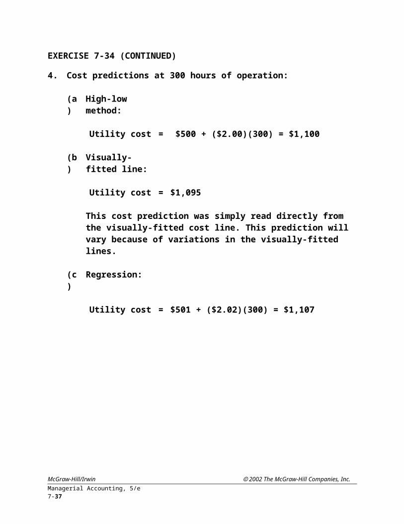
EXERCISE 7-34 (CONTINUED)
4. Cost predictions at 300 hours of operation:
(a) High-low method:
Utility cost = $500 + ($2.00)(300) = $1,100
(b) Visually-fitted line:
Utility cost = $1,095
This cost prediction was simply read directly from the visually-fitted cost line. This prediction will vary because of variations in the visually-fitted lines.
(c) Regression:
Utility cost = $501 + ($2.02)(300) = $1,107
McGraw-Hill/Irwin 2002 The McGraw-Hill Companies, Inc.7-26 Solutions Manual
SOLUTIONS TO PROBLEMS
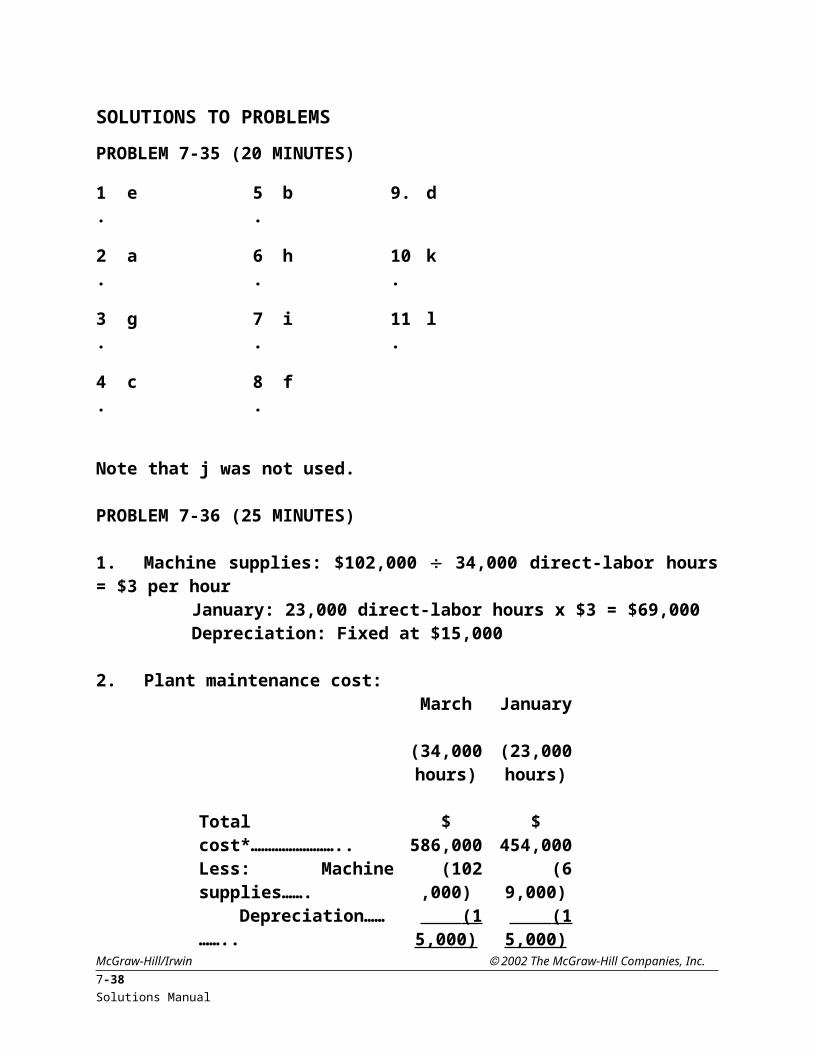
PROBLEM 7-35 (20 MINUTES)
1. e 5. b 9. d
2. a 6. h 10. k
3. g 7. i 11. l
4. c 8. f
Note that j was not used.
PROBLEM 7-36 (25 MINUTES)
1. Machine supplies: $102,000 34,000 direct-labor hours = $3 per hourJanuary: 23,000 direct-labor hours x $3 = $69,000Depreciation: Fixed at $15,000
2. Plant maintenance cost:March
(34,000 hours)
January
(23,000 hours)
Total cost*…………………….. $ 586,000 $ 454,000Less: Machine supplies……. (102,000) (69,000)
Depreciation………….. (15,000) (15,000) Plant maintenance…………... $ 469,000 $ 370,000
* Excludes supervisory labor cost
Variable maintenance cost = difference in cost difference in direct-labor hours
= ($469,000 – $370,000) (34,000 – 23,000)= $99,000 11,000 hours= $9 per hour
McGraw-Hill/Irwin 2002 The McGraw-Hill Companies, Inc.Managerial Accounting, 5/e 7-27

PROBLEM 7-36 (CONTINUED)
Fixed maintenance cost:March(34,000 hours)
January (23,000 hours)
Total maintenance cost………………. $469,000 $370,000Less: Variable cost at $9 per hour…. 306,000 207,000 Fixed maintenance cost……………… $163,000 $163,000
3. Manufacturing overhead at 29,500 labor hours:
Machine supplies at $3 per hour……. $ 88,500Depreciation……………………………. 15,000Plant maintenance cost:
Variable at $9 per hour…………… 265,500Fixed…………………………………. 163,000
Supervisory labor……………………… 90,000 Total…………………………….. $622,000
4. A fixed cost remains constant when a change occurs in the cost driver (or activity base). A step-fixed cost, on the other hand, remains constant within a range but will change (rise or fall) when activity falls outside that range.
5. Ideally, the company should operate on the right-most portion of a step, just prior to the jump in cost. In this manner, a firm receives maximum benefit (i.e., the maximum amount of activity) for the dollars invested.
PROBLEM 7-37 (25 MINUTES)
1. Straight-line depreciation—committed fixedCharitable contributions—discretionary fixedMining labor/fringe benefits—variableRoyalties—semivariableTrucking and hauling—step-fixedThe per-ton mining labor/fringe benefit cost is constant at both volume levels presented, which is characteristic of a variable cost.
$345,000 1,500 tons = $230 per ton$598,000 2,600 tons = $230 per ton
McGraw-Hill/Irwin 2002 The McGraw-Hill Companies, Inc.7-28 Solutions Manual
PROBLEM 7-37 (CONTINUED)
Royalties have both a variable and a fixed component, making it a semivariable (mixed) cost.
Variable royalty cost = difference in cost difference in tons= ($201,000 – $135,000) (2,600 – 1,500)= $66,000 1,100 tons= $60 per ton
Fixed royalty cost:June
(2,600 tons)December
(1,500 tons)
Total royalty cost………………………. $201,000 $135,000Less: Variable cost at $60 per ton….. 156,000 90,000 Fixed royalty cost……………………… $ 45,000 $ 45,000
2. Total cost for 1,650 tons:
Depreciation…………………………………………... $ 25,000Charitable contributions……………………………. ----Mining labor/fringe benefits at $230 per ton……. 379,500Royalties:
Variable at $60 per ton………………………….. 99,000Fixed……………………………………………….. 45,000
Trucking and hauling……………………………….. 275,000 Total……………………………………………….. $823,500
3. Hauling 1,500 tons is not very cost effective. Antioch will incur cost of $275,000 if it needs 1,500 tons hauled or, for that matter, 1,899 tons. The company would be better off if it had 1,499 tons hauled, saving outlays of $25,000. In general, with this type of cost function, effectiveness is maximized if a firm operates on the right-most portion of a step, just prior to a jump in cost.
2. A committed fixed cost results from an entity’s ownership or use of facilities and its basic organizational structure. Examples of such costs include property taxes, depreciation, rent, and management salaries. Discretionary fixed costs, on the other hand, arise from a decision to spend a particular amount of money for a specific purpose. Outlays for research and development, advertising, and charitable contributions fall in this category.
McGraw-Hill/Irwin 2002 The McGraw-Hill Companies, Inc.Managerial Accounting, 5/e 7-29

PROBLEM 7-37 (CONTINUED)
In times of severe economic difficulties, management should try to cut discretionary fixed costs. Such costs are more easily altered in the short run and do not have significant long-term ramifications for a firm. The decision to close a manufacturing facility, for example, could reduce property taxes, rent, and/or depreciation. However, that decision may result in a significant long-run change in operations that may be difficult to overturn when economic conditions rebound.
5. Antioch uses a calendar year for tax-reporting purposes. At year-end, it may have ample funds available and decide to make donations to charitable causes. Such contributions are deductible in computing the company’s tax obligation to the government. Tax deductions reduce taxable income and, therefore, produce a tax savings for the firm.
PROBLEM 7-38 (25 MINUTES)
1. Variable maintenance cost per hour of service =
= $7.50
Total maintenance cost at 300 hours of service......................................... $2,820Variable maintenance cost at 300 hours of service (300 hr. $7.50)...... 2,250Fixed maintenance cost per month............................................................. $ 570
Cost formula:
Monthly maintenance cost = $570 + $7.50X, where X denotes hours of maintenance service.
2. The variable component of the maintenance cost is $7.50 per hour of service.
3. Cost prediction at 590 hours of activity:
Maintenance cost = $570 + ($7.50)(590) = $4,995
McGraw-Hill/Irwin 2002 The McGraw-Hill Companies, Inc.7-30 Solutions Manual
PROBLEM 7-38 (CONTINUED)
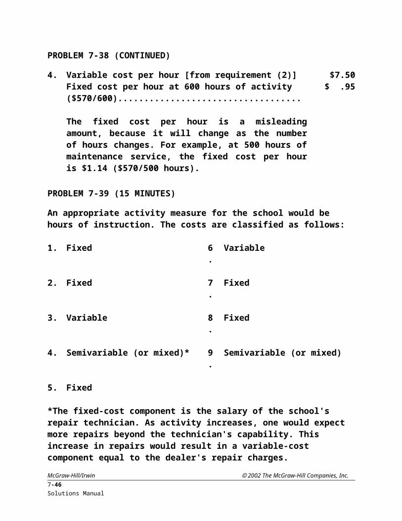
4. Variable cost per hour [from requirement (2)]............................................ $7.50Fixed cost per hour at 600 hours of activity ($570/600)............................. $ .95
The fixed cost per hour is a misleading amount, because it will change as the number of hours changes. For example, at 500 hours of maintenance service, the fixed cost per hour is $1.14 ($570/500 hours).
PROBLEM 7-39 (15 MINUTES)
An appropriate activity measure for the school would be hours of instruction. The costs are classified as follows:
1. Fixed 6. Variable
2. Fixed 7. Fixed
3. Variable 8. Fixed
4. Semivariable (or mixed)* 9. Semivariable (or mixed)
5. Fixed
*The fixed-cost component is the salary of the school's repair technician. As activity increases, one would expect more repairs beyond the technician's capability. This increase in repairs would result in a variable-cost component equal to the dealer's repair charges.
McGraw-Hill/Irwin 2002 The McGraw-Hill Companies, Inc.Managerial Accounting, 5/e 7-31

PROBLEM 7-40 (40 MINUTES)
McGraw-Hill/Irwin 2002 The McGraw-Hill Companies, Inc.7-32 Solutions Manual
Total course maintenance cost
$12,500
$12,400
$12,300
$12,200
$12,100
$12,000
0 50 100 150 200 250 300
Number of golfers
Fixedcomponent
ofmaintenance
cost
The lower part of thevertical axis has been
shortened.
Semivariablecost approximation
Step-variablecomponent
of maintenancecost
1.
1.
2.

PROBLEM 7-40 (CONTINUED)
3. Fixed-cost component = $12,010
Variable-cost component:
Variable cost per golfer =
= $2
Cost equation:
Maintenance cost per month = $12,010 + $2X, where X denotes the number of golfers during the month.
4. Predicted Course Maintenance Costs
Using Fixed Cost Coupled
with Step-Variable Cost
Behavior Pattern
Using Semivariable Cost
Approximation150 people tee off................................ $12,300 $12,310158 people tee off................................ 12,320 12,326
McGraw-Hill/Irwin 2002 The McGraw-Hill Companies, Inc.Managerial Accounting, 5/e 7-33

PROBLEM 7-41 (40 MINUTES)
McGraw-Hill/Irwin 2002 The McGraw-Hill Companies, Inc.7-34 Solutions Manual
$12,500
Material-handling costs
$12,000
$11,500
$11,000
$10,500
$10,000
$9,500
500 1,000 1,500 2,000 2,500
Control factorunits
The lower part of the vertical axis has been shortened.
2.
Visually-fitted cost line
PROBLEM 7-41 (CONTINUED)
2. See graph for requirement (1).
3. The estimate of the fixed cost is the intercept on the vertical axis.
Fixed-cost component = $9,700
To estimate the variable-cost component, choose any two points on the visually-fitted cost line. For example, choose the following points:
Activity Cost0................................................................................................ $ 9,7002,000......................................................................................... 11,700
Then proceed as follows to estimate the variable-cost component:
Variable cost per control factor unit =
= $1.00
4. Cost equation:
Total material-handling cost = $9,700 + $1.00X, where X denotes the number of control factor units of activity during the month.
5. High-low method:
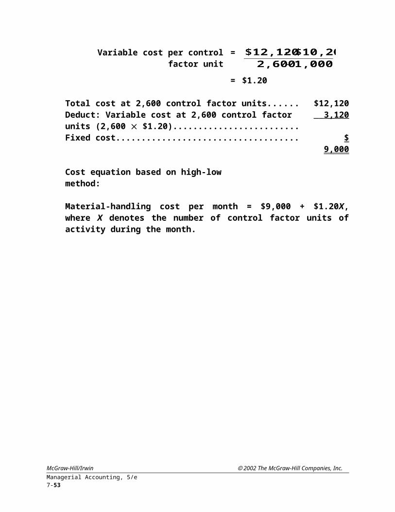
Variable cost per control factor unit =
= $1.20
Total cost at 2,600 control factor units......................................................... $12,120Deduct: Variable cost at 2,600 control factor units (2,600 $1.20).......... 3,120 Fixed cost......................................................................................................... $ 9,000
Cost equation based on high-low method:
Material-handling cost per month = $9,000 + $1.20X, where X denotes the number of control factor units of activity during the month.
McGraw-Hill/Irwin 2002 The McGraw-Hill Companies, Inc.Managerial Accounting, 5/e 7-35

PROBLEM 7-41 (CONTINUED)
6. Memorandum
Date: Today
To: President, Martha’s Vineyard Marine Supply
From: I.M. Student
Subject: Material-handling cost estimates
On the basis of a scatter diagram and visually-fitted cost line, the Material-Handling Department's monthly cost behavior was estimated as follows:
Material-handling cost per month = $9,700 + $1.00 per control factor unit
A control factor unit is defined in this department as 100 pounds of equipment loaded or unloaded at the loading dock.
Using the high-low method, the following cost estimate was obtained:
Material-handling cost per month = $9,000 + $1.20 per control factor unit
The two methods yield different estimates because the high-low method uses only two data points, ignoring the rest of the information. The method of visually fitting a cost line, while subjective, uses all of the data available.
In this case, the two data points used by the high-low method do not appear to be representative of the entire set of data.
7. Predicted Material-Handling Costs
Using Visually-FittedCost Line*
UsingHigh-Low Method
$12,000 = $9,700 + ($1.00)(2,300) $11,760 = $9,000 + ($1.20)(2,300)
*This method is preferable, because it uses all of the data.
McGraw-Hill/Irwin 2002 The McGraw-Hill Companies, Inc.7-36 Solutions Manual
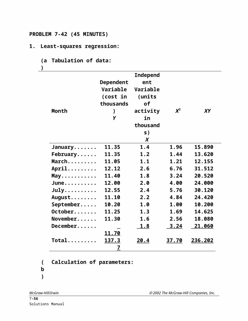
PROBLEM 7-42 (45 MINUTES)
1. Least-squares regression:
(a) Tabulation of data:
Month
Dependent Variable (cost in
thousands)Y
Independent Variable (units of
activity in thousands)
X X2 XYJanuary....................... 11.35 1.4 1.96 15.890February...................... 11.35 1.2 1.44 13.620March........................... 11.05 1.1 1.21 12.155April............................. 12.12 2.6 6.76 31.512May.............................. 11.40 1.8 3.24 20.520June............................. 12.00 2.0 4.00 24.000July.............................. 12.55 2.4 5.76 30.120August......................... 11.10 2.2 4.84 24.420September................... 10.20 1.0 1.00 10.200October....................... 11.25 1.3 1.69 14.625November.................... 11.30 1.6 2.56 18.080December.................... 11.70 1.8 3.24 21.060Total............................. 137.37 20.4 37.70 236.202
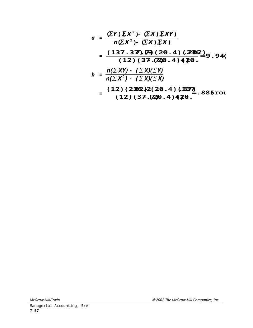
(b) Calculation of parameters:
a =
=
b =
=
McGraw-Hill/Irwin 2002 The McGraw-Hill Companies, Inc.Managerial Accounting, 5/e 7-37
PROBLEM 7-42 (CONTINUED)
(c) Fixed- and variable-cost components:
Monthly fixed cost = $9,943*
Variable cost = $.89 per control factor unit (rounded)†
*The intercept parameter (a) computed above is the cost per month in thousands.†The slope parameter (b) calculated above is the cost in thousands of dollars per thousand units of activity. Equivalently, it is the cost per unit of activity.
2. Total monthly cost = $9,943 + $.89 per control factor unit
3. Cost prediction for 2,300 control factor units of activity:
Total monthly cost = $9,943 + ($.89)(2,300) = $11,990
4. The cost predictions differ because the cost formulas differ under the three cost-estimation methods. The high-low method, while objective, uses only two data points.Ten observations are excluded.
The visual-fit method, while it uses all of the data, is somewhat subjective. Different analysts may draw different cost lines.
Least-squares regression is objective, uses all of the data, and is a statistically sound method of estimation.
Therefore, least-squares regression is the preferred method of cost estimation.
McGraw-Hill/Irwin 2002 The McGraw-Hill Companies, Inc.7-38 Solutions Manual

PROBLEM 7-43 (25 MINUTES)
1. Scatter diagrams:
Present, in graphic form, the relationship between costs and cost drivers via a plot of data points
Require that a straight line be fit through the data points, with approximately the same number of data points above and below the line
Easy to use Provide a means to easily recognize outliers
Least-squares regression:
Uses statistical formulas to fit a cost line through the data points Is a very objective method of cost estimation that uses all the data points Requires more computation than other cost-estimation methods; however, software
programs are readily available
High-low method:
Relies on only two data points (for the highest and lowest activity levels) in drawing conclusions about cost behavior
Is considered more objective than the scatter diagram; however, is weaker than the scatter diagram because it relies on only two data points
The least-squares regression method will typically produce the most accurate results.
2. Yes. The three methods produce equations by different means. Scatter diagrams and least-squares regression rely on an examination of all data points. The scatter diagram, however, requires an analyst to fit a line through the points by visual approximation, or “eyeballing.” In contrast, least-squares regression involves the use of statistical formulas to derive the best possible fit of the line through the points. Finally, the high-low method is based on an analysis of only two data points: the highest and the lowest activity levels.
McGraw-Hill/Irwin 2002 The McGraw-Hill Companies, Inc.Managerial Accounting, 5/e 7-39

PROBLEM 7-43 (CONTINUED)
3. These amounts represent the fixed and variable cost associated with the ticketing operation. Fixed cost totals $312,000 within the relevant range, and Global American incurs $2.30 of variable cost for each ticket issued.
4. C = $320,000 + $2.15PTC = $320,000 + ($2.15 x 580,000)C = $1,567,000
5. Yes, she did err by including November data. November is not representative because of the effects of the Delta Western strike. The month is an outlier and should be eliminated from the data set.
6. Currently, most of the airline’s tickets are written through reservations personnel, whose wages are likely variable in nature. Heavier reliance on the Internet means a greater investment in software, Web-site maintenance and development, and other similar expenditures. Outlays that fall in these latter categories are typically fixed costs, assuming that the cost driver is the number of tickets. The outcome would parallel the experiences of a manufacturing firm that automates its processes and reduces its reliance on direct-labor personnel.
McGraw-Hill/Irwin 2002 The McGraw-Hill Companies, Inc.7-40 Solutions Manual

PROBLEM 7-44 (35 MINUTES)
1. The regression equation's intercept on the vertical axis is $200. It represents the portion of indirect material cost that does not vary with machine hours when operating within the relevant range. The slope of the regression line is $4 per machine hour. For every machine hour, $4 of indirect material costs are expected to be incurred.
2. Estimated cost of indirect material at 900 machine hours of activity:
S = $200 + ($4 900)
= $3,800
3. Several questions should be asked:
(a) Do the observations contain any outliers, or are they all representative of normal operations?
(b) Are there any mismatched time periods in the data? Are all of the indirect material cost observations matched properly with the machine hour observations?
(c) Are there any allocated costs included in the indirect material cost data?
(d) Are the cost data affected by inflation?
4.April August
Beginning inventory.............................................................. $1,200 $ 950+ Purchases........................................................................... 6,000 6,100 – Ending inventory................................................................ (1,550) (2,900)Indirect material used........................................................... $5,650 $4,150
5. High-low method:
Variable cost per machine hour
=
=
PROBLEM 7-44 (CONTINUED)
Fixed cost per month:
McGraw-Hill/Irwin 2002 The McGraw-Hill Companies, Inc.Managerial Accounting, 5/e 7-41

Total cost at 1,100 hours................................................................................ $5,650Variable cost at 1,100 hours
($5 1,100).............................................................................................. 5,500Fixed cost......................................................................................................... $ 150
Equation form:
Indirect material cost = $150 + ($5 machine hours)
6. The regression estimate should be recommended because it uses all of the data, not just two pairs of observations.
PROBLEM 7-45 (40 MINUTES)
1. The original method was simply the average overhead per hour for the last 12 months and did not distinguish between fixed and variable costs. Rand divided total overhead by total labor hours, which effectively treated all overhead as variable. Regression analysis measures the behavior of the overhead costs in relation to labor hours and is a model that distinguishes between fixed and variable costs within the relevant range of 2,500 to 7,500 labor hours.
2. a. Based on the regression analysis, the variable cost per person for a cocktail party is $22, calculated as follows:
Food and beverages................................................................................ $15Labor (.5 hr. @ $10/hr.)............................................................................ 5Variable overhead (.5 hr. @ $4/hr.)......................................................... 2
Total..................................................................................................... $22
b. Based on the regression analysis, the full absorption cost per person for a cocktail party is $27, calculated as follows:
Food and beverages................................................................................ $15Labor (.5 hr. @ $10/hr.)............................................................................ 5Variable overhead (.5 hr. @ $4/hr.)......................................................... 2Fixed overhead (.5 hr. @ $10/hr.)*.......................................................... 5
Total..................................................................................................... $27
McGraw-Hill/Irwin 2002 The McGraw-Hill Companies, Inc.7-42 Solutions Manual

PROBLEM 7-45 (CONTINUED)
*$48,000 x 12 months = $576,000 $576,000/57,600 hr. = $10/hr.
3. The minimum bid for a 200-person cocktail party would be $4,400. The amount is calculated by multiplying the variable cost per person of $22 by 200 people. At any price above the variable cost, Dana Rand will be earning a contribution toward her fixed costs.
4. Other factors that Dana Rand should consider in developing a bid include the following:
The assessment of the current capacity of her business. If the business is at capacity, other work would have to be sacrificed at some opportunity cost.
Analyses of the competition. If competition is rigorous, she may not have much bargaining power.
A determination of whether or not her bid will set a precedent for lower prices.
The realization that regression analysis is based on historical data, and that any anticipated changes in the cost structure should be considered.
McGraw-Hill/Irwin 2002 The McGraw-Hill Companies, Inc.Managerial Accounting, 5/e 7-43

PROBLEM 7-46 (45 MINUTES)
Month
Applications Received
(in thousands)X
Cost of Operating the Admissions
Office (in thousands)
Y X2 XYAugust......................... 20 8.9 400 178.0September................... 30 10.0 900 300.0October....................... 25 9.6 625 240.0November.................... 22 9.1 484 200.2December.................... 15 8.7 225 130.5January....................... 10 8.0 100 80.0 Total............................. 122 54.3 2,734 1,128.7
a. Least-squares regression:
7.076* =
.097* =
Total monthly admissions department costs = $7,076 + $.097X, where X denotes the number of applications in thousands.
*Rounded.
McGraw-Hill/Irwin 2002 The McGraw-Hill Companies, Inc.7-44 Solutions Manual

PROBLEM 7-46 (CONTINUED)
b. High-low method:
Variable cost per thousand applications =
= $.10
Total cost at 30 thousand applications............................................. $10,000Variable cost at 30 thousand applications (30,000 $.10)............. 3,000 Fixed cost per month........................................................................... $ 7,000
Total monthly admissions department costs = $7,000 + $.10X
c. Visual-fit method:
Total monthly admissions department costs = $7,100 + $.095X
McGraw-Hill/Irwin 2002 The McGraw-Hill Companies, Inc.Managerial Accounting, 5/e 7-45
PROBLEM 7-47 (45 MINUTES)
1. Scatter diagram:
Note: Only 11 data points appear, because two monthly observations were identical (May and September).
McGraw-Hill/Irwin 2002 The McGraw-Hill Companies, Inc.7-46 Solutions Manual
Airport costs
$30,000
$25,000
$20,000
$15,000
$10,000
$5,000
250 500 750 1,000 1,250 1,500 1,750
Flights

PROBLEM 7-47 (CONTINUED)
2. Least-squares regression:
(a) Tabulation of data:
Month
Dependent Variable (cost in
thousands)Y
Independent Variable
(flights in hundreds)
X X2 XYJanuary....................... 20 11 121 220February...................... 17 8 64 136March........................... 19 14 196 266April............................. 18 9 81 162May.............................. 19 10 100 190June............................. 20 12 144 240July.............................. 18 11 121 198August......................... 24 14 196 336September................... 19 10 100 190October....................... 21 12 144 252November.................... 17 9 81 153December.................... 21 15 225 315 Total............................. 233 135 1,573 2,658
(b) Calculation of parameters:
a =
=
b =
=
McGraw-Hill/Irwin 2002 The McGraw-Hill Companies, Inc.Managerial Accounting, 5/e 7-47
PROBLEM 7-47 (CONTINUED)
(c) Fixed- and variable-cost components:
Monthly fixed cost = $11,796
Variable cost = $677 per hundred flights
3. Cost equation:
Total monthly airport cost = $11,796 + $677X, where X denotes the number of flights in hundreds.
4. Cost prediction for 1,600 flights:
Airport cost for the month = $11,796 + ($677)(16) = $22,628
5. Calculation and interpretation of R 2:
(a) Formula for calculation:
where Y denotes the observed value of the dependent variable (cost) at a particular activity level.
Y ' denotes the predicted value of the dependent variable (cost) based on the regression line, at a particular activity level.
denotes the mean (average) observation of the dependent variable (cost).
McGraw-Hill/Irwin 2002 The McGraw-Hill Companies, Inc.7-48 Solutions Manual

PROBLEM 7-47 (CONTINUED)
(b) Tabulation of data:*
Month Y X
Predicted Cost (in thousands)Based on
RegressionLine Y' [( Y– Y')2]† [(Y – )2]†
January.......... 20 11 19.243 .573 .340February......... 17 8 17.212 .045 5.842March.............. 19 14 21.274 5.171 .174April................ 18 9 17.889 .012 2.008May................. 19 10 18.566 .188 .174June................ 20 12 19.920 .006 .340July................. 18 11 19.243 1.545 2.008August............ 24 14 21.274 7.431 21.004September...... 19 10 18.566 .188 .174October.......... 21 12 19.920 1.166 2.506November....... 17 9 17.889 .790 5.842December....... 21 15 21.951 .904 2.506Total................ 18.019 42.918
*Y' = ($11,796 + $677X)/$1,000= Y/12 = 233/12 = 19.417 (rounded)
†Rounded.
(c) Calculation of R2:
R2 = 1 – = .58 (rounded)
McGraw-Hill/Irwin 2002 The McGraw-Hill Companies, Inc.Managerial Accounting, 5/e 7-49

PROBLEM 7-47 (CONTINUED)
(d) Interpretation of R2:
The coefficient of determination, R2, is a measure of the goodness of fit of the least-squares regression line. An R2 of .58 means that 58% of the variability of the dependent variable about its mean is explained by the variability of the independent variable about its mean. The higher the R2, the better the regression line fits the data. The interpretation of a high R2 is that the independent variable is a good predictor of the behavior of the dependent variable. In the county’s cost estimation, a high R2 would mean that the county budget officer can be relatively confident in the cost predictions based on the estimated-cost behavior pattern. An R2 of .58 is not particularly high.
McGraw-Hill/Irwin 2002 The McGraw-Hill Companies, Inc.7-50 Solutions Manual

SOLUTIONS TO CASES
CASE 7-48 (45 MINUTES)
1. Cairns' preliminary estimate for overhead of $18.00 per direct-labor hour does not distinguish between fixed and variable overhead. This preliminary rate is applicable only to the activity level at which it was computed (36,000 direct-labor hours per year) and may not be used to predict total overhead at other activity levels.
The overhead rate developed from the least-squares regression recognizes the relationship between cost and volume in the data. The regression suggests that there is a component of the cost ($26,200 per month) that is unrelated to total direct-labor hours. This cost component is the intercept on the vertical axis and is often considered to be the fixed cost as long as the activity level is within the relevant range. Thus, the least-squares regression results in a cost function with two components: fixed cost per month and variable cost per direct-labor hour. This cost formula can be used to predict total overhead at any activity level.
2. Direct material................................................................................................ $400.00Direct labor (5 DLH* $10.00 per DLH)....................................................... 50.00Variable overhead (5 DLH $9.25 per DLH)............................................... 46.25Total variable cost per 1,000 square feet..................................................... $496.25
*DLH denotes direct-labor hour.
3. The minimum bid should include the following incremental costs of the project.:
Direct material ($400.00 60)...................................................................... $24,000Direct labor ($50.00 60)............................................................................. 3,000Variable overhead ($9.25 per DLH 5 DLH 60)..................................... 2,775Overtime premium ($5.00 per DLH 5 DLH 60 .4)............................ 600Minimum bid................................................................................................... $30,375
4. Yes, Cairns can rely on the formula as long as she recognizes that there are some shortcomings. The fact that least-squares regression estimates cost behavior increases the usefulness of rates computed from cost data. However, the regression is based on historical costs that may change in the future, and Cairns must assess whether the cost equation would need to be revised for future cost increases or decreases.
McGraw-Hill/Irwin 2002 The McGraw-Hill Companies, Inc.Managerial Accounting, 5/e 7-51

CASE 7-48 (CONTINUED)
5. a. Variable OH1 (60 5 $4.10)...................................................................... $1,230Variable OH2 (60 $13.50)............................................................................ 810Variable OH3 (80 $6.60).............................................................................. 528 Total incremental variable overhead............................................................ $2,568
b. Variable OH1 (60 5 $4.10)...................................................................... $1,230Variable OH2 (30 $13.50)............................................................................ 405Variable OH3 (250 $6.60)............................................................................ 1,650Total incremental variable overhead............................................................ $3,285
c. The two scenarios in (a) and (b) differ in terms of the activities to be undertaken. Scenario (a) involves a large amount of seeding activity and relatively little planting activity. Scenario (b) involves considerably less seeding activity, but a great deal more planting activity. An activity-based costing system accounts for the different costs in projects involving different mixes of activity.
McGraw-Hill/Irwin 2002 The McGraw-Hill Companies, Inc.7-52 Solutions Manual
CASE 7-49 (45 MINUTES)
1. Scatter diagram:
2. through 4. See scatter diagram for requirement (1).
McGraw-Hill/Irwin 2002 The McGraw-Hill Companies, Inc.Managerial Accounting, 5/e 7-53
Administrative cost
$25,000
$20,000
$15,000
$10,000
$5,000
500 1,000 1,500 2,000Patient load
Visually-fitted semivariable
cost line
Visually-fitted curvilinear cost line
Relevant range3.
2.
4.
CASE 7-49 (CONTINUED)
5. Fixed cost = $6,900
6. Administrative cost = $6,900 + $3.08X, where X denotes the number of patients.
7. Cost predictions:
PatientLoad
Cost Prediction
800............................ $9,300300............................ 4,000
It makes no difference which cost line is used to make the cost prediction for 800 patients. The semivariable approximation is very accurate at this patient load, which is near the middle of the relevant range. However, for a patient load of 300 patients, the curvilinear cost line yields a much more accurate prediction.
CASE 7-50 (50 MINUTES)
1. High-low method:
Variable administrative cost per patient =
Total cost at 1,500 patients............................................................................ $16,100Variable cost at 1,500 patients....................................................................... 15,000Fixed cost per month...................................................................................... $ 1,100
Cost formula:
Total monthly administrative cost = $1,100 + $10X, where X denotes the number of patients for the month.
The variable cost per patient is $10.
McGraw-Hill/Irwin 2002 The McGraw-Hill Companies, Inc.7-54 Solutions Manual

CASE 7-50 (CONTINUED)
2. Least-squares regression:
(a) Tabulation of data:
Month
Dependent Variable (cost in
hundreds)Y
Independent Variable
(patients in hundreds)
X X2 XYJanuary....................... 139 14 196 1,946February...................... 70 5 25 350March........................... 60 4 16 240April............................. 100 10 100 1,000May.............................. 119 13 169 1,547June............................. 92 9 81 828July.............................. 102 11 121 1,122August......................... 41 3 9 123September................... 94 7 49 658October....................... 111 12 144 1,332November.................... 83 6 36 498December.................... 161 15 225 2,415 Total............................. 1,172 109 1,171 12,059
(b) Calculation of parameters:
a =
=
b =
=
McGraw-Hill/Irwin 2002 The McGraw-Hill Companies, Inc.Managerial Accounting, 5/e 7-55
CASE 7-50 (CONTINUED)
(c) Cost behavior in formula form (with rounded parameters):*
Total monthly administrative cost = $2,671 + $7.81X, where X denotes the number of patients for the month.
*When interpreting the regression parameters, remember that both the cost and patient data were transformed to hundreds. Thus, the 26.707 intercept parameter (a) is in terms of hundreds of dollars of cost, or $2,671 (rounded). The 7.812 slope parameter (b) is in terms of hundreds of dollars of cost per hundred patients, or $781 (rounded) per hundred patients. This amount is equivalent to $7.81 per patient.
(d) The variable cost per patient is $7.81, as explained above.
3. MemorandumDate: Today
To: Jeffrey Mahoney, Administrator
From: I.M. Student
Subject: Comparison of cost estimates for clinic administrative costs
Three alternative cost-estimation methods were used to estimate the pediatric clinic's administrative cost behavior. The results of these three approaches (in formula form) are shown below. In each formula, X denotes the number of patients in a month.
(a) Least-squares regression method:
Total monthly administrative cost = $2,671 + $7.81X
(b) High-low method:
Total monthly administrative cost = $1,100 + $10X
McGraw-Hill/Irwin 2002 The McGraw-Hill Companies, Inc.7-56 Solutions Manual
CASE 7-50 (CONTINUED)
(c) Visual-fit method:
Total monthly administrative cost = $6,900 + $3.08X
These cost estimates differ very significantly. The activity level in the clinic during its first year of operation fluctuated greatly. This fluctuation is not expected in the future; patient loads in the range of 600 to 1,200 patients per month are anticipated.
The cost estimates differ so greatly because two of the methods (least-squares and high-low) used data from outside the relevant range of activity. The clinic's administrative cost behavior appears from the scatter diagram to be curvilinear over the entire range. The cost behavior pattern exhibits very low costs in the range of activity below the relevant range and very high costs in the activity range above the relevant range. Since the regression and high-low estimates are so heavily influenced by observations outside the relevant range, they do not provide the best estimate in this case of how administrative costs are likely to behave within the relevant range. In this instance, the visually-fitted cost line probably provides the best estimate. The visually-fitted cost line has a much flatter slope than the other two cost lines, indicating that total variable administrative costs will probably rise at about $3.25 per patient.
Another possible approach would be to use least-squares regression, but restrict the data to those observations within the relevant range. However, only a handful of observations would remain to include in the analysis.
My overall recommendation is to use the visually-fitted cost line as the best estimate until the clinic has operated for its second year. Then I would recommend a new cost analysis using least-squares regression on all of the data from the relevant range of activity.
McGraw-Hill/Irwin 2002 The McGraw-Hill Companies, Inc.Managerial Accounting, 5/e 7-57
CASE 7-50 (CONTINUED)
4. It is very inappropriate for the hospital administrator to manipulate the cost information supplied by the controller in order to push his own agenda before the board of trustees. It is the board's legitimate role to decide whether or not to establish and continue operations in the clinic. In making decisions about the clinic, the board should have the best information possible, including the controller's best estimate as to how administrative costs will behave.
Megan McDonough, the hospital’s Director of Cost Management, has a professional obligation to provide her best professional judgment to the board of trustees. The standards of ethical conduct for management accountants include the following requirements concerning objectivity:
(a) Communicate information fairly and objectively.
(b) Disclose fully all relevant information that could reasonably be expected to influence an intended user's understanding of the reports, comments, and recommendations presented.
McDonough should insist that the best and most appropriate estimate of the clinic's administrative cost behavior be presented to the board.
McGraw-Hill/Irwin 2002 The McGraw-Hill Companies, Inc.7-58 Solutions Manual
CURRENT ISSUES IN MANAGERIAL ACCOUNTING
ISSUE 7-51
"DRUG-PRICE PROGRAM NOTES," THE WALL STREET JOURNAL, AUGUST 10, 2000.
1. A fixed cost is a cost that will not change in total as production levels change within the relevant range. Common examples include straight-line depreciation, supervisory salaries, and rent. The pharmaceutical industry has high fixed costs and low variable costs. Its high fixed costs are “baked in the cake” because of the research and development necessary to yield a profitable drug. Therefore, research and development is a fixed cost of the drug industry. Variable costs are low because, after the discovery and approval process has been completed, it's not very expensive to manufacture the pills.
2. A variable cost is a cost that will change in total as production levels change. Direct material and electricity are often classified as variable costs. Many costs are semivariable (or mixed); they contain both variable and fixed cost components.
ISSUE 7-52
"DELTA, NORTHWEST POST STRONG NET DESPITE FUEL COSTS, HIGHER FARES," THE WALL STREET JOURNAL, JULY 21, 2000, MARTHA BRANNIGAN AND MICHAEL J. MCCARTHY.
1. Fuel costs are variable. The distance flown, as well as the weight of the cargo and/or passengers, determines how much fuel is used during a flight.
2. An airline would benefit from estimating costs since management needs cost information to schedule routes and determine the sales price of tickets.
ISSUE 7-53
"AIRBUS 'CRUISE SHIP IN THE SKY'," THE WALL STREET JOURNAL, AUGUST 30, 2000, JEFF COLE AND DANIEL MICHAELS.
1. Significantly different costs would be the variable costs per passenger such as fuel, food, and personnel costs for the flight attendants. Increased costs of hangar space due to the size of the plane would be considered fixed costs.
2. Maintenance costs for a new aircraft are always difficult to predict.
3. An airline would benefit from estimating costs. Management needs cost estimates to schedule routes and to determine the sales price of tickets.
McGraw-Hill/Irwin 2002 The McGraw-Hill Companies, Inc.Managerial Accounting, 5/e 7-59

ISSUE 7-54
"DELTA PILOTS' UNION PROPOSES PAY RAISES MAKING SALARIES HIGHER THAN UNITED'S," THE WALL STREET JOURNAL, OCTOBER 16, 2000, MARTHA BRANNIGAN.
1. Pilots' salaries are considered a fixed cost of a particular flight, in the sense that the cost would not vary with respect to the number of passengers. However, pilots’ salaries do vary with the number of flights and their length.
2. An airline would benefit from estimating costs. Management needs cost estimates to schedule routes and to determine the sales price of tickets.
ISSUE 7-55
"HOSPITALS IN NH POST MORE LOSSES," THE WALL STREET JOURNAL, APRIL 26, 2000, JAMES BANDLER.
1. Fixed costs are costs that remain the same in total as the volume of activity changes.
2. Sharing laboratory expenses with other hospitals would be an example of a way to reduce fixed costs.
ISSUE 7-56
"HOLLYWOOD RUSHES TO BEAT A STRIKE," BUSINESS WEEK, JANUARY 8, 2001, RONALD GROVER.
1. Will Smith will receive $20 million and 20% of revenues. This is a semivariable cost.
2. Colin Farrell will receive $2.5 million for Tigerland. This is a fixed cost.
McGraw-Hill/Irwin 2002 The McGraw-Hill Companies, Inc.7-60 Solutions Manual