Software defined radio design for synchronization of 802 ... · Software defined radio design for...
103
Calhoun: The NPS Institutional Archive Theses and Dissertations Thesis Collection 2007-09 Software defined radio design for synchronization of 802.11A receiver Sanfuentes, Juan L. Monterey, California. Naval Postgraduate School http://hdl.handle.net/10945/3197
Transcript of Software defined radio design for synchronization of 802 ... · Software defined radio design for...
Calhoun: The NPS Institutional Archive
Theses and Dissertations Thesis Collection
2007-09
Software defined radio design for synchronization of
802.11A receiver
Sanfuentes, Juan L.
Monterey, California. Naval Postgraduate School
http://hdl.handle.net/10945/3197
NAVAL
POSTGRADUATE SCHOOL
MONTEREY, CALIFORNIA
THESIS
Approved for public release; distribution is unlimited
SOFTWARE DEFINED RADIO DESIGN FOR SYNCHRONIZATION OF 802.11A RECEIVER
by
Juan Luis Sanfuentes
September 2007
Thesis Advisor: Frank Kragh Second Reader: Roberto Cristi

THIS PAGE INTENTIONALLY LEFT BLANK
i
REPORT DOCUMENTATION PAGE Form Approved OMB No. 0704-0188 Public reporting burden for this collection of information is estimated to average 1 hour per response, including the time for reviewing instruction, searching existing data sources, gathering and maintaining the data needed, and completing and reviewing the collection of information. Send comments regarding this burden estimate or any other aspect of this collection of information, including suggestions for reducing this burden, to Washington headquarters Services, Directorate for Information Operations and Reports, 1215 Jefferson Davis Highway, Suite 1204, Arlington, VA 22202-4302, and to the Office of Management and Budget, Paperwork Reduction Project (0704-0188) Washington DC 20503. 1. AGENCY USE ONLY (Leave blank)
2. REPORT DATE September 2007
3. REPORT TYPE AND DATES COVERED Master’s Thesis
4. TITLE AND SUBTITLE: Software Defined Radio Design for Synchronization of 802.11a Receiver 6. AUTHOR(S) Juan Luis Sanfuentes
5. FUNDING NUMBERS
7. PERFORMING ORGANIZATION NAME(S) AND ADDRESS(ES) Naval Postgraduate School Monterey, CA 93943-5000
8. PERFORMING ORGANIZATION REPORT NUMBER
9. SPONSORING /MONITORING AGENCY NAME(S) AND ADDRESS(ES) N/A
10. SPONSORING/MONITORING AGENCY REPORT NUMBER
11. SUPPLEMENTARY NOTES The views expressed in this thesis are those of the author and do not reflect the official policy or position of the Department of Defense or the U.S. Government. 12a. DISTRIBUTION / AVAILABILITY STATEMENT Approved for public release; distribution is unlimited.
12b. DISTRIBUTION CODE
13. ABSTRACT (maximum 200 words) Constant improvements in techniques applied to different radio communication system stages, including coding, modulation, synchronization and security, make any implementation quickly obsolete. On the other hand, different communication standards used among military and public safety agencies make difficult the necessary interoperability. These reasons force users to replace equipment frequently, increasing cost and implementation time. Software Defined Radios (SDRs), partly implemented in software, can solve these problems, making full use of programmable modules. This thesis presents an implementation of the necessary algorithms that solve the synchronization requirements of IEEE 802.11a WLAN receivers. This is a continuation of a previous thesis effort, where the post-synchronization steps of the receiver were addressed. The software utilized for this purpose is the Open Source SCA Implementation::Embedded (OSSIE), developed by Virginia Tech. Each algorithm was created as a different component, allowing reuse and modularity for the development of future waveforms.
15. NUMBER OF PAGES
102
14. SUBJECT TERMS Software Defined Radio, IEEE 802.11, LAN, Synchronization, OFDM, OSSIE, CORBA.
16. PRICE CODE
17. SECURITY CLASSIFICATION OF REPORT
Unclassified
18. SECURITY CLASSIFICATION OF THIS PAGE
Unclassified
19. SECURITY CLASSIFICATION OF ABSTRACT
Unclassified
20. LIMITATION OF ABSTRACT
UU NSN 7540-01-280-5500 Standard Form 298 (Rev. 2-89) Prescribed by ANSI Std. 239-18

ii
THIS PAGE INTENTIONALLY LEFT BLANK
iii
Approved for public release; distribution is unlimited
SOFTWARE DEFINED RADIO DESIGN FOR SYNCHRONIZATION OF 802.11A RECEIVER
Juan L. Sanfuentes
Lieutenant Commander, Chilean Navy B. Electrical Engineering, Naval Engineering School, 1997
Submitted in partial fulfillment of the requirements for the degree of
MASTER OF SCIENCE IN ELECTRICAL ENGINEERING
from the
NAVAL POSTGRADUATE SCHOOL September 2007
Author: Juan L. Sanfuentes
Approved by: Assistant Professor Frank Kragh Thesis Advisor
Professor Roberto Cristi Second Reader
Professor Jeffrey B. Knorr Chairman, Department of Electrical and Computer Engineering .

iv
THIS PAGE INTENTIONALLY LEFT BLANK
v
ABSTRACT
Constant improvements in techniques applied to different radio communication
system stages, including coding, modulation, synchronization and security, make any
implementation quickly obsolete. On the other hand, different communication standards
used among military and public safety agencies make difficult the necessary
interoperability. These reasons force users to replace equipment frequently, increasing
cost and implementation time. Software Defined Radios (SDRs), partly implemented in
software, can solve these problems, making full use of programmable modules. This
thesis presents an implementation of the necessary algorithms that solve the
synchronization requirements of IEEE 802.11a WLAN receivers. This is a continuation
of a previous thesis effort, where the post-synchronization steps of the receiver were
addressed. The software utilized for this purpose is the Open Source SCA
Implementation: Embedded (OSSIE), developed by Virginia Tech. Each algorithm was
created as a different component, allowing reuse and modularity for the development of
future waveforms.

vi
THIS PAGE INTENTIONALLY LEFT BLANK
vii
TABLE OF CONTENTS
I. INTRODUCTION........................................................................................................1 A. OBJECTIVES ..................................................................................................1 B. CONTRIBUTIONS..........................................................................................1 C. RELATED WORKS........................................................................................2
1. OSSIE....................................................................................................2 2. OFDM Synchronization ......................................................................3
D. THESIS ORGANIZATION............................................................................3
II. BACKGROUND ..........................................................................................................5 A. SOFTWARE BASED RADIO (SBR).............................................................5
1. Software Defined Radio (SDR) ...........................................................5 2. Software Communication Architecture.............................................6 3. Open Source SCA Implementation: Embedded (OSSIE)................6
B. OFDM SYNCHRONIZATION ......................................................................7 1. OFDM Fundamentals..........................................................................7 2. Synchronization..................................................................................11
a. Packet Detection......................................................................11 b. Symbol Timing ........................................................................13 c. Frequency Synchronization....................................................14 d. Carrier Phase Tracking ..........................................................16 e. Channel Estimation ................................................................17
C. IEEE 802.11A .................................................................................................18 1. Modulation Scheme ...........................................................................19 2. Packet Structure.................................................................................20
a. PHY for OFDM System Description......................................20 b. OFDM Specific Service Parameters.......................................21
D. CHAPTER SUMMARY................................................................................22
III. SIMULATIONS AND DESIGN ...............................................................................23 A. MATLAB SIMULATION.............................................................................23
1. Transmitter.........................................................................................23 2. Channel ...............................................................................................25 3. Receiver...............................................................................................26 4. Results .................................................................................................27
a. AWGN......................................................................................27 b. Frequency Offset.....................................................................28 c. Multipath .................................................................................29
B. OSSIE DESIGN .............................................................................................33 1. Design Considerations .......................................................................33
a. Components.............................................................................33 b. Ports.........................................................................................33 c. Properties.................................................................................34
2. Synchronization Components Structure..........................................35
viii
IV. OSSIE COMPONENT DEVELOPMENT..............................................................37 A. SYNCHRONIZATION COMPONENT DEVELOPMENT......................37
1. Component Development Using OSSIE...........................................37 2. Synchronization Stage Components.................................................39
a. Delay and Correlate ................................................................40 b. Symbol Timing ........................................................................43 c. Frequency Synchronization....................................................45 d. Channel Estimation ................................................................47 e. FFT..........................................................................................48 f. Buffer Size ...............................................................................50 g. CP Removal .............................................................................51 h. Channel Compensation ..........................................................52 i. Phase Tracking .......................................................................54
B. ISSUES DURING DEVELOPMENT AND RECOMMENDATIONS.....55 1. OSSIE Installation .............................................................................55 2. Documentation ...................................................................................56
a. Assembly Controller Component............................................56 b. FFTW Library.........................................................................57
V. 802.11A WAVEFORM AND TESTING..................................................................59 A. 802.11A SYNCHRONIZATION WAVEFORM.........................................59 B. TESTING WAVEFORMS............................................................................61
1. Test 0 ...................................................................................................62 2. Test 1 ...................................................................................................63 3. Test 2 ...................................................................................................63 4. Test 3 ...................................................................................................64
C. RESULTS .......................................................................................................64 1. Signal 1................................................................................................66 2. Signal 2................................................................................................67 3. Signal 3................................................................................................69 4. Signal 4................................................................................................70 5. Signal 5................................................................................................72 6. Signal 6................................................................................................73
VI. CONCLUSIONS AND FUTURE WORK...............................................................77 A. SUMMARY OF WORK................................................................................77 B. SUGGESTED FUTURE WORK .................................................................77
1. Demodulation and Codification Components Upgrade .................77 a. Initialization Circuit................................................................78 b. Connection Between Synchronization and Decoding
Components.............................................................................78 2. Real Data Test ....................................................................................78
LIST OF REFERENCES......................................................................................................79
INITIAL DISTRIBUTION LIST .........................................................................................81
ix
LIST OF FIGURES
Figure 1. OFDM symbol generation. (After Ref. [14])....................................................8 Figure 2. CP generation (After Ref. [14]). ........................................................................9 Figure 3. Delayed sub-carrier without CP (After Ref. [13]). ..........................................10 Figure 4. Delayed sub-carrier with CP (After Ref. [13]). ...............................................10 Figure 5. Block diagram of the delay and correlate algorithm (From Ref. [15]). ..........12 Figure 6. Block diagram of correlation based algorithm.................................................13 Figure 7. Analytic signal. ................................................................................................14 Figure 8. PPDU frame format. (After Ref. [17]).............................................................20 Figure 9. PLCP preamble. (After Ref. [17])....................................................................21 Figure 10. Block diagram of the Matlab simulation program...........................................23 Figure 11. Received signal after downconversion. ...........................................................26 Figure 12. Signal affected by a frequency offset of 140 kHz............................................29 Figure 13. Signal affected by a frequency offset of 170 kHz............................................29 Figure 14. Signal with a second path delayed 0.6 sµ . ......................................................31 Figure 15. Signal with a second path delayed 1.2 sµ ........................................................32 Figure 16. Sample component communication layouts (From Ref. [18]).........................34 Figure 17. Block diagram of OFDM synchronization waveform. ....................................35 Figure 18. OWD Man Machine Interface. ........................................................................38 Figure 19. Flowchart symbol definitions. .........................................................................39 Figure 20. Delay_Corr component flowchart. ..................................................................42 Figure 21. Symbol_Timing component flowchart. ............................................................44 Figure 22. F_Sync component flowchart. .........................................................................46 Figure 23. Channel_Estimation component flowchart......................................................48 Figure 24. FFT component flowchart. ..............................................................................49 Figure 25. Buffer_Size component flowchart. ...................................................................51 Figure 26. CP_Removal component flowchart. ................................................................52 Figure 27. CH_C component flowchart. ...........................................................................53 Figure 28. Phase_Trk component flowchart. ....................................................................55 Figure 29. 802.11a component core structure. ..................................................................59 Figure 30. General model of synchronization stage waveform.........................................60 Figure 31. Initialization circuit..........................................................................................61 Figure 32. Test 0 waveform. .............................................................................................62 Figure 33. Test 1 waveform. .............................................................................................63 Figure 34. Test 2 waveform. .............................................................................................63 Figure 35. Test 3 waveform. .............................................................................................64 Figure 36. Frequency synchronization effect in Signal 1..................................................66 Figure 37. Channel and phase correction of Signal 1........................................................67 Figure 38. Frequency synchronization effect in Signal 2..................................................68 Figure 39. Channel and phase correction of Signal 2........................................................68 Figure 40. Frequency synchronization effect in Signal 3..................................................69 Figure 41. Channel and phase correction of Signal 3........................................................70 Figure 42. Frequency synchronization effect in Signal 4..................................................71
x
Figure 43. Channel and phase correction of Signal 4........................................................71 Figure 44. Frequency synchronization effect in Signal 5..................................................72 Figure 45. Channel and phase correction of Signal 5........................................................73 Figure 46 Frequency synchronization effect in Signal 6..................................................74 Figure 47. Channel and phase correction of Signal 6........................................................75
xi
LIST OF TABLES
Table 1. Rate Dependent Parameters (After Ref. [17])..................................................19 Table 2. Non-zero values of P sequence........................................................................21 Table 3. Pilot value designation example. .....................................................................22 Table 4. Sub-carriers position of OFDM symbols (After Ref. [17]). ............................24 Table 5. List of functions defined in the Tx block.........................................................25 Table 6. List of functions defined in Channel block......................................................25 Table 7. List of functions defined in the Rx block.........................................................26 Table 8. Characteristics of the simulated 802.11a signals. ............................................65

xii
THIS PAGE INTENTIONALLY LEFT BLANK
xiii
LIST OF SYMBOLS, ACRONYMS AND ABBREVIATIONS
ADC Analog to Digital Converter AWGN Additive White Gaussian Noise CP Cyclic Prefix DSW Double Sliding Window FFT Fast Fourier Transform FPGA Field Programmable Gate Array ICI Intercarrier Interference IF Intermediate Frequency IFFT Inverse Fast Fourier Transform ISI Intersymbol Interference JPEO Joint Program Executive Office JTRS Joint Tactical Radio System LP Long Preamble MAC Medium Access Control MMI Man Machine Interface OFDM Orthogonal Frequency Division Multiplexing OSSIE Open Source SCA Implementation::Embedded OWD OSSIE Waveform Developer PHY Physical Layer PLCP PHY Layer Convergence Procedure PPDU PLCP Protocol Data Unit PSDU PHY Layer Service Data Unit PSK Phase Shift Keying QAM Quadrature Amplitude Modulation SBR Software Based Radio SCA Software Communication SDR Software Defined Radio SP Short Preamble TS Training Sequence USB Universal Serial Bus WLAN Wireless Local Area Networks WNW Wideband Network Waveform

xiv
THIS PAGE INTENTIONALLY LEFT BLANK
xv
EXECUTIVE SUMMARY
This thesis presents a Software Defined Radio (SDR) application for a particular
communication system, the synchronization stage of an Orthogonal Frequency Division
Multiplexing (OFDM) packet based receiver. The standard chosen for this work is the
IEEE 802.11a standard, which specifies Wireless Local Area Network (WLAN)
operation in the 5 GHz band. A SDR solution refers to the capacity to reprogram the
hardware involved in a communication system, in order to manage different waveforms.
The main advantage is the ability to modify the system’s characteristics, including
modulation, error control coding, carrier frequency and data link protocol, while avoiding
the necessity of changing the hardware. This is essential in the military, since disparate
equipment, with its particular characteristics and lack of modularity, makes
interoperability between branches and allied countries difficult. This new concept has
been of great interest in the U.S. Government, where the Joint Tactical Radio System
(JTRS), a major program conducted by the Joint Program Executive Office (JPEO), has
developed an open source framework denominated the Software Communication
Architecture (SCA), which defines the way to configure hardware and software that form
a SDR system.
The software utilized for developing the application is the Open Source SCA
Implementation::Embedded (OSSIE), a SDR design environment created by Mobile and
Portable Radio Research Group (MPRG) based at Virginia Tech University. This
software facilitates the design of software components that perform a particular
communication task, and the design of waveforms based on the interconnection and
configuration of these components.
The synchronization stage of 802.11a extends the functionality of an already
developed thesis, which covered the post synchronization stage: signal demodulation and
decoding. That work assumed an ideal channel and perfect synchronization and was
developed in an earlier version of OSSIE. OFDM has become an attractive alternative for
new communication standards due largely to its efficient use of the spectrum, achieving
considerable bandwidth efficiency, thereby allowing wireless transmission at high data
xvi
rates in a modest bandwidth. A foundational concept behind OFDM is the use of
orthogonal sub-carriers that split the transmitted data into different channels, after
performing an Inverse Fast Fourier Transform (IFFT), allowing parallel transmission
with no self-interference. The use of a Cyclic Prefix (CP) before each OFDM symbol,
which consists of the repetition of the symbol tail, allows robustness against multipath
due to IFFT properties. Synchronization is crucial with OFDM for successfully receiving
the transmitted signal, since the orthogonality can be lost because of incorrect packet
detection, symbol synchronization, or a frequency offset.
The synchronization process performed in this application includes coarse and
fine packet start detection, coarse and fine frequency detection and correction, channel
estimation and compensation, and finally symbol phase tracking and correction. The use
of Matlab, a programming language oriented towards engineering calculations, at the
beginning of the work was essential for verifying the correct implementation of the
algorithms obtained from the literature. After this process, the next step was
programming the components in OSSIE and testing them against the results obtained in
Matlab. The testing was achieved by creating a waveform that includes the developed
components, which processed simulated OFDM signals generated in Matlab. These
simulated signals were affected by noise, frequency offset and a multipath channel. The
results demonstrated the correct functionality of the components by verifying the digital
samples after each component through the use of constellation diagrams.
Future work in this specific implementation includes the development of a
component in charge of controlling the necessary hardware to obtain the digital samples
that should be passed to the first component in the synchronization stage: the packet
detection. Also, work is needed in revising the demodulation and decoding stage
components in order to make them compatible with the current version of OSSIE and
integrate them with the synchronization components developed in this thesis, obtaining a
complete 802.11a receiver working in OSSIE. Finally, work is needed to integrate the
software solution onto a suitable hardware platform, in particular one capable of
processing the high data rate OFDM signal in real time.
xvii
ACKNOWLEDGMENTS
I would like to thank Professor Frank Kragh for the opportunity to work in the
area of Software Defined Radio, a subject that is of great interest in the communications
community and will help me in my current and future job. His guidance during the
development of the thesis and patience in the revision process were invaluable.
Professor Roberto Cristi motivated me to work with OFDM. His course in Digital
Signal Processing for Wireless Communication presented the fundamental concepts of
this modern communication waveform in a very professional and enjoyable class. He also
constantly supported me in answering innumerable questions and kept my own spot on
his blackboard for almost a year.
Donna Miller was a great help at NPS’s Software Defined Radio Laboratory. She
quickly and efficiently assisted me in solving all of the hardware and software requests I
brought her.
I would like to thank the constant support of my wife Paola and my daughter
Constanza, who had the patience and understanding that allowed me to finish this
challenge.

xviii
THIS PAGE INTENTIONALLY LEFT BLANK
1
I. INTRODUCTION
A. OBJECTIVES
The purpose of this thesis is to demonstrate that different components of a radio
communication system can be made reconfigurable using software. In particular this
work has the following objectives:
• Understand the concepts of SDR and learn how to use OSSIE as a platform to create communication components, and design a desired waveform.
• Learn the synchronization techniques useful for OFDM signals. • Apply these synchronization algorithms, using the development tool
included in OSSIE. • Prove the functionality of each component, by testing the corresponding
waveform by receiving OFDM packets affected by the channel.
B. CONTRIBUTIONS
The present thesis contributes to several organizations, where the use of SDR is
becoming important. OFDM synchronization is not only used in 802.11a, but also in
others standards including:
• IEEE 802.11g Wireless Local Area Network in the 2.4 GHz band [1], • IEEE 802.16 Wireless Metropolitan Area Network, • European Telecommunications Standards Institute (ETSI) Technical
Report (TR) 101 496 Digital Audio Broadcasting (DAB), • ETSI European Standard (EN) 301 701 Digital Video Broadcasting
(DVB), and • International Telecommunications Union (ITU) G-992 Asymmetric
Digital Subscriber Line (ADSL).
OFDM is currently used also in the military. An example of this is the Wideband
Network Waveform (WNW) [2]. Due to the current success OFDM is undergoing, it
seems very likely that future standards will implement it as its principal modulation
scheme.
2
The immediate contribution of this thesis is to increase the library of components
under development for the OSSIE community, where Virginia Tech and NPS are
collaborating.
The U.S. government is publishing standards, including Software Communication
Architecture (SCA) [3], to guide the industry in the development of software defined
radio communication systems. The open source feature of OSSIE, allows the industry to
use components already developed.
Due to several naval exercises that American and allied navies execute every
year, there is a permanent requirement of interoperability, which is achieved by following
common tactical procedures and using compatible communication systems. The use of
SDR is a valuable alternative to perform the necessary configurations to achieve the
required compatibility, avoiding changes in hardware. This thesis contributes to allied
navies that have not considered or have just started using SDR in their communication
systems, giving them the basic knowledge in this area, and providing them with some
components that will permit future developments.
C. RELATED WORKS
1. OSSIE
Since OSSIE has been available as a tool that allows development of SDR
systems, several works have been executed. The major efforts come from the group that
created and continuously upgraded the software: Mobile and Portable Radio Research
Group (MPRG) from Virginia Tech [4].
Motivated by research and educational needs, and considering the next generation
in communication systems that U.S. Government Institutions will operate, NPS currently
is offering a SDR course, which is supported by a dedicated laboratory. As a
consequence, some theses have been developed in this area, where OSSIE is the adopted
software platform. SDR designs have been produced at NPS for:
3
• IS 95B – The Code Division Multiple Access (CDMA)-based 2G cellular
phone standard in North America [5].
• IEEE 802.16- A standard for wireless Metropolitan Area Networks [6].
• IEEE 802.11a- An amendment to a wireless Local Area Network standard [7].
The 802.11a thesis work by Leong [7] was developed using OSSIE version 0.5.0,
where the different stages needed in both the transmitter and receiver were considered.
The receiver uses a total of 18 components for demodulation and decoding, assuming an
ideal channel. Simulations were completed, where the obtained results demonstrated the
correct functionality of the corresponding components.
The natural next step related to 802.11a receivers is the development of the
synchronization stage and channel correction, the subject of the present thesis.
2. OFDM Synchronization
A recent work in OFDM synchronization at NPS is the thesis by Sardana [8],
where packet and frequency detection methods were evaluated. Some recommendations
in this work emphasize the use of data aided based algorithms. In the case of frequency
synchronization, it is shown that the two-step estimation, first coarse and then fine
detection, is effective. This is accomplished using both short and long training sequences,
as will be described later.
D. THESIS ORGANIZATION
The remaining chapters are organized as follows:
• Chapter II explains all the concepts related to OFDM synchronization and SDR in order to understand the basis of the current work.
• Chapter III explains the design of the algorithms for synchronization, and the simulation results. The main goal of this chapter is to verify the correct functionality of the algorithms.
4
• Chapter IV examines the application developed in OSSIE, where the development of each particular component is explained.
• Chapter V provides the test results using different 802.11a signals, previously generated in Matlab.
• Chapter VII gives conclusions and discusses recommendations for future work in this particular waveform.
5
II. BACKGROUND
A. SOFTWARE BASED RADIO (SBR)
The concept behind SBR is the capacity to reprogram the hardware involved in a
communication system, in order to manage different communication waveforms, as
required. The main advantage is the ability to modify the system’s characteristics,
including modulation, error control coding, carrier frequency and data link protocol,
while avoiding the necessity of exchanging the hardware.
The term SBR is used in a generic way to describe this emerging technology, where the terms Software Defined Radio (SDR) and Software Radio (SR) are used depending on the specific stage, within a communication system, where this technology is applied. [9]
1. Software Defined Radio (SDR)
As introduced in the last paragraph, the terms SDR and SR are part of this
software based technology. SDR refers to certain communication tasks that are developed
in software; including, in the receiver case, the processing performed after the down
conversion process. Software Radio (SR), on the other hand, implies an almost totally
software-based solution, where the digitization step occurs as close to the antenna as
possible, and all the following steps are developed and managed using software. [9]
SDR is a relatively new area that has been growing, and should be seen as part of
the fast development of wireless communications. New technology has helped this quick
technical evolution including, among others, the processor’s speed. The flexibility of
software based implementations makes this alternative an excellent choice to ameliorate
the issues that have been raised, including compatibility with recent technology and the
desirability of hardware reuse.
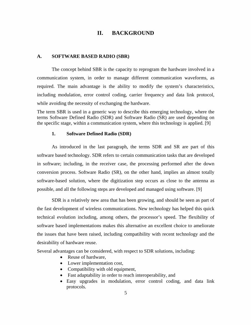
Several advantages can be considered, with respect to SDR solutions, including: • Reuse of hardware, • Lower implementation cost, • Compatibility with old equipment, • Fast adaptability in order to reach interoperability, and • Easy upgrades in modulation, error control coding, and data link
protocols.
6
2. Software Communication Architecture
The Software Communication Architecture (SCA) is an open source framework
that defines the way to configure the hardware and software that form a SDR system [10].
A framework is a set of classes that work together for a specific type of software. Using
support programs like libraries, it is designed to facilitate software development.
The SCA is mandated by the Joint Tactical Radio System (JTRS), a major
program conducted by the Joint Program Executive Office (JPEO) JTRS, which develops
solutions intended to satisfy DoD communication interoperability requirements.
Flexibility and platform independence are the main characteristics of the SCA,
which allows modularity and facilitates application development. On the other hand, the
idea of developing applications independent of the hardware, where at least one General
Purpose Processor (GPP) is available, come at the cost of some inefficiencies, including
memory allocation problems and latency. [11]
3. Open Source SCA Implementation: Embedded (OSSIE)
OSSIE is open-source SDR development software. It is a current project
developed by Mobile and Portable Radio Research Group (MPRG) based at Virginia
Tech University. Created as a solution to implement communication waveforms, it allows
SDR application development that follows the SCA specifications. The project is written
in the computer languages C++ and python and it has been under continuous
development, since 2003 [12]. The goals of OSSIE are based in investigation and
educational purposes, from the study of interoperability issues to the training of students
in the concepts and development of SDR.
An important tool of OSSIE is the OSSIE Waveform Developer (OWD), which is
supporting software that enables rapid design of components and waveforms.
Components are applications that execute a specific task in a communication system
chain. Selecting the necessary components, the OWD allows the development of a
specific type of waveform.
7
B. OFDM SYNCHRONIZATION
OFDM signals are used both in broadcast as well as in packet switched
transmissions, with different synchronization requirements. In the broadcast case, the
receiver has a relatively long period of time for synchronization, whereas in packet
systems, time is limited and a fast synchronization is required before and during each
packet [13]. Due to differences in this time constraint, the applied algorithms are not the
same.
Wireless Local Area Networks (WLANs) are packet switched systems; thus, the
following explanation refers to algorithms used in these types of networks.
1. OFDM Fundamentals
OFDM signals allow splitting a high data rate stream into a parallel number of
slow data rate streams, which are transmitted through orthogonal carrier frequencies. The
effect of the slow data rate due to the increase in symbol duration is the reduction of the
fraction of the symbol duration affected by signal dispersion in time caused by multipath
delay spread. At the same time, the bandwidth of each sub-carrier is smaller compared to
the channel bandwidth, thus the usual frequency selective fading on the entire 802.11a
band is realized as flat fading of each sub-carrier, which is much easier to equalize [14].
Several difficulties arise when utilizing digital multicarrier modulation
techniques, including intersymbol interference (ISI) and intercarrier interference (ICI).
The former is almost eliminated by using a guard time before every OFDM symbol. The
latter is avoided applying a cyclic prefix of the symbol in the guard time, keeping the
orthogonality between sub-carriers. [13]
The way to generate an OFDM symbol involves a coding process that ends with a
digital modulation mapping, using either Phase Shift Keying (PSK) or Quadrature
Amplitude Modulation (QAM) on each sub-carrier. Then an Inverse Fast Fourier
Transform (IFFT) over a defined number of values is performed, which has the effect of
modulating each sub-carrier’s symbol by the appropriate complex exponential to create a
8
complex envelope signal where the symbols are orthogonally frequency division
multiplexed with minimally spaced frequencies, for maximum spectral efficiency.
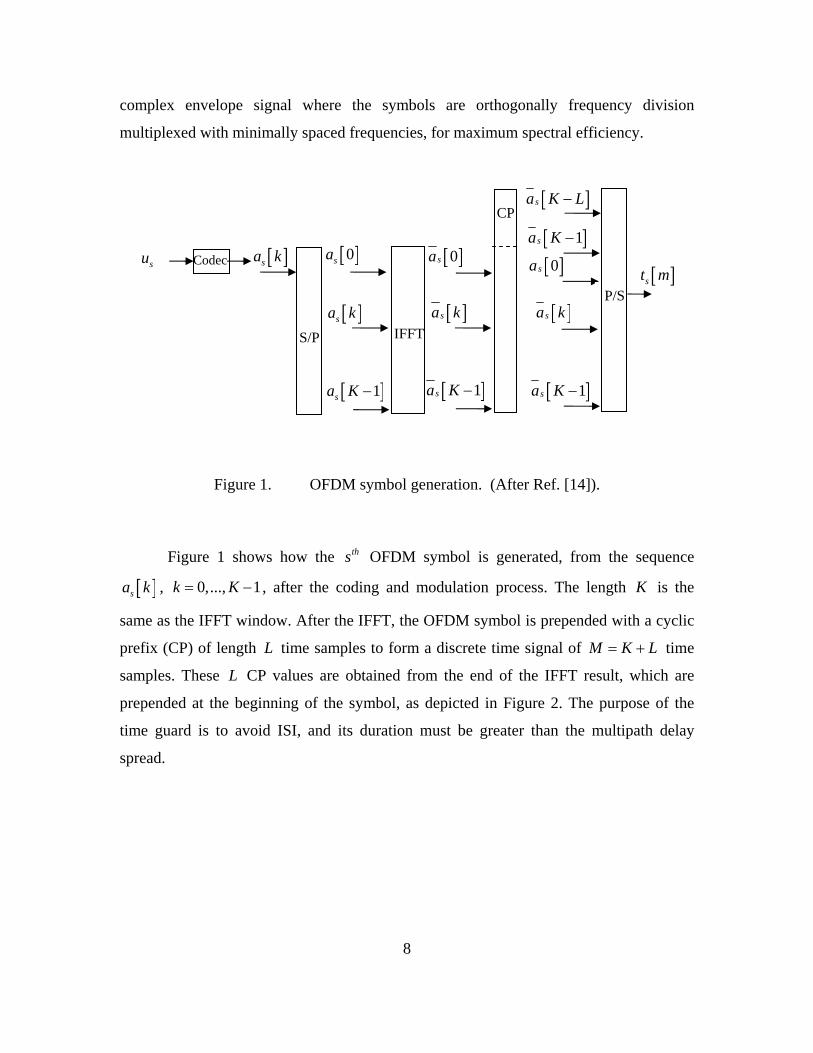
Figure 1. OFDM symbol generation. (After Ref. [14]).
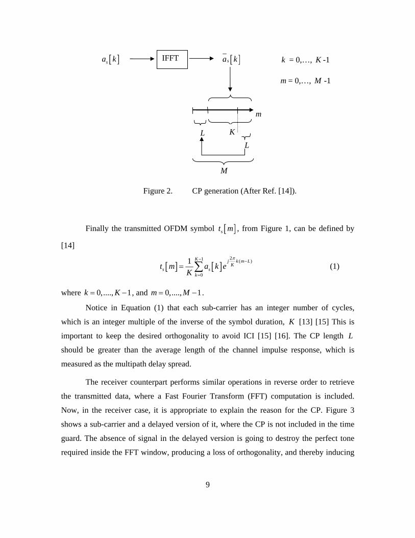
Figure 1 shows how the ths OFDM symbol is generated, from the sequence
[ ]sa k , 0,..., 1k K= − , after the coding and modulation process. The length K is the
same as the IFFT window. After the IFFT, the OFDM symbol is prepended with a cyclic
prefix (CP) of length L time samples to form a discrete time signal of M K L= + time
samples. These L CP values are obtained from the end of the IFFT result, which are
prepended at the beginning of the symbol, as depicted in Figure 2. The purpose of the
time guard is to avoid ISI, and its duration must be greater than the multipath delay
spread.
CP
Codec [ ]sa k
[ ]sa k
[ ]st m
[ ]1sa K −
[ ]0sa
[ ]1sa K −
[ ]sa K L−
[ ]1sa K −
IFFT
[ ]0sa
[ ]1sa K −
[ ]sa k
[ ]0sa
S/P
su
P/S [ ]sa k
9
Figure 2. CP generation (After Ref. [14]).
Finally the transmitted OFDM symbol [ ]st m , from Figure 1, can be defined by
[14]
[ ] [ ]21 ( )
0
1 K j k m LK
s sk
t m a k eK
π− −
=
= ∑ (1)
where 0,...., 1k K= − , and 0,...., 1m M= − .
Notice in Equation (1) that each sub-carrier has an integer number of cycles,
which is an integer multiple of the inverse of the symbol duration, K [13] [15] This is
important to keep the desired orthogonality to avoid ICI [15] [16]. The CP length L
should be greater than the average length of the channel impulse response, which is
measured as the multipath delay spread.
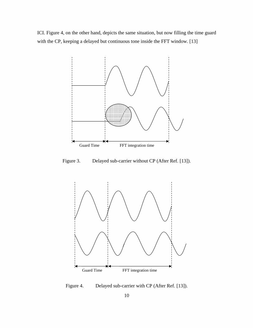
The receiver counterpart performs similar operations in reverse order to retrieve
the transmitted data, where a Fast Fourier Transform (FFT) computation is included.
Now, in the receiver case, it is appropriate to explain the reason for the CP. Figure 3
shows a sub-carrier and a delayed version of it, where the CP is not included in the time
guard. The absence of signal in the delayed version is going to destroy the perfect tone
required inside the FFT window, producing a loss of orthogonality, and thereby inducing
M
L
m
[ ]sa k [ ]sa k IFFT
KL
k = 0,…, K -1
m = 0,…, M -1
10
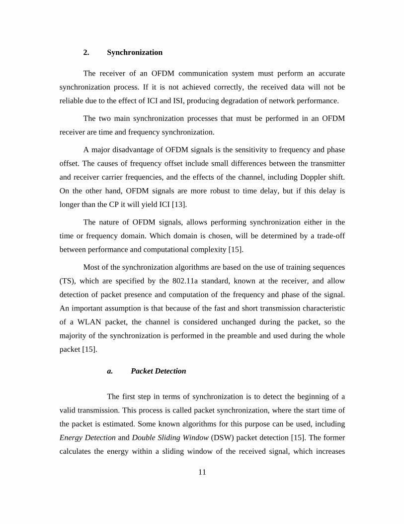
ICI. Figure 4, on the other hand, depicts the same situation, but now filling the time guard
with the CP, keeping a delayed but continuous tone inside the FFT window. [13]
Figure 3. Delayed sub-carrier without CP (After Ref. [13]).
Figure 4. Delayed sub-carrier with CP (After Ref. [13]).
Guard Time FFT integration time
Guard Time FFT integration time
11
2. Synchronization
The receiver of an OFDM communication system must perform an accurate
synchronization process. If it is not achieved correctly, the received data will not be
reliable due to the effect of ICI and ISI, producing degradation of network performance.
The two main synchronization processes that must be performed in an OFDM
receiver are time and frequency synchronization.
A major disadvantage of OFDM signals is the sensitivity to frequency and phase
offset. The causes of frequency offset include small differences between the transmitter
and receiver carrier frequencies, and the effects of the channel, including Doppler shift.
On the other hand, OFDM signals are more robust to time delay, but if this delay is
longer than the CP it will yield ICI [13].
The nature of OFDM signals, allows performing synchronization either in the
time or frequency domain. Which domain is chosen, will be determined by a trade-off
between performance and computational complexity [15].
Most of the synchronization algorithms are based on the use of training sequences
(TS), which are specified by the 802.11a standard, known at the receiver, and allow
detection of packet presence and computation of the frequency and phase of the signal.
An important assumption is that because of the fast and short transmission characteristic
of a WLAN packet, the channel is considered unchanged during the packet, so the
majority of the synchronization is performed in the preamble and used during the whole
packet [15].
a. Packet Detection
The first step in terms of synchronization is to detect the beginning of a
valid transmission. This process is called packet synchronization, where the start time of
the packet is estimated. Some known algorithms for this purpose can be used, including
Energy Detection and Double Sliding Window (DSW) packet detection [15]. The former
calculates the energy within a sliding window of the received signal, which increases
12
when a packet is received. A decision is made based on a predefined threshold. In the
DSW packet detection case, the energy in two consecutives sliding windows is
calculated. The difference yields an impulse when the packet begins. The drawback of
the first method is the complexity in setting the energy threshold that decides whether the
incoming signal level indicates the start of a valid packet or not. This is largely because
the noise power and the signal power are usually not known beforehand.
Although DSW packet detection is a good solution, better results are
obtained if known information is considered, taking advantage of the cross-correlation
properties that give a result independent of the power. This known information is the
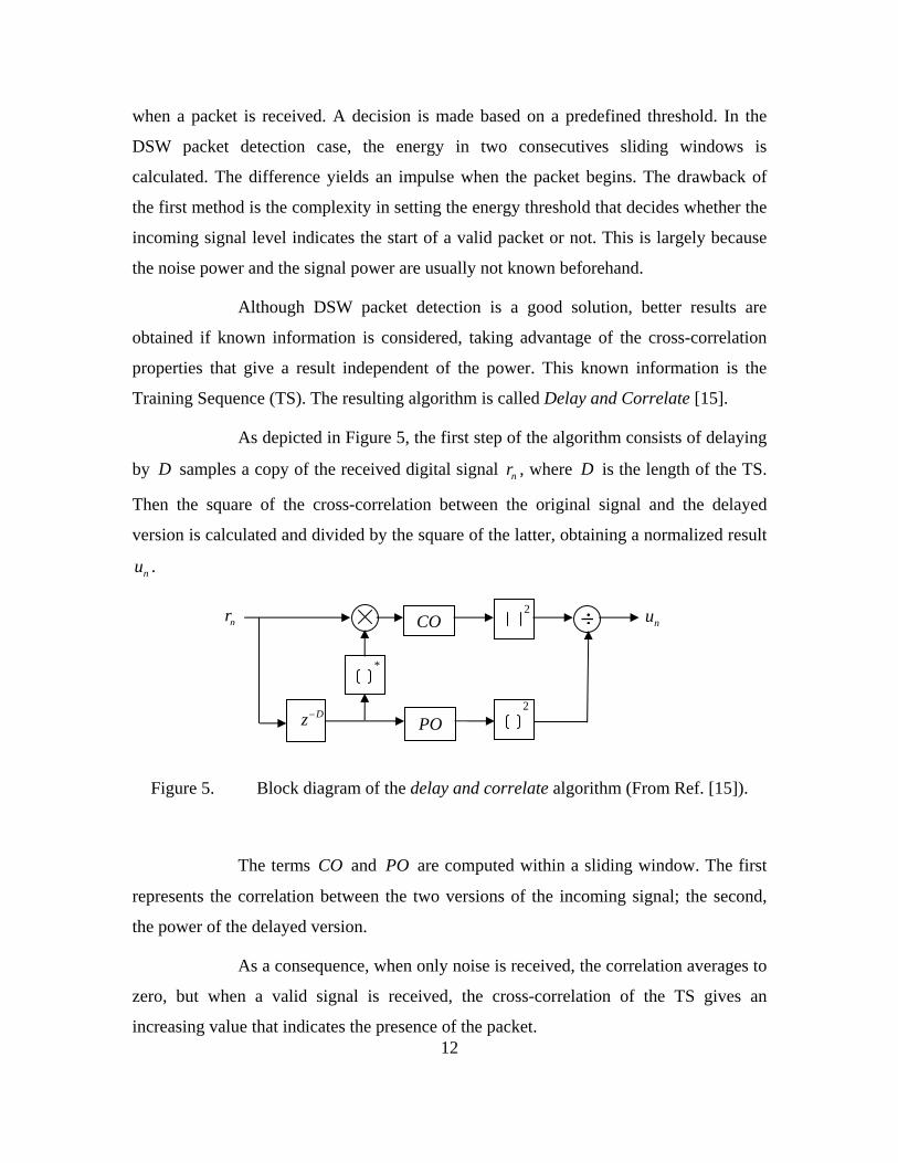
Training Sequence (TS). The resulting algorithm is called Delay and Correlate [15].
As depicted in Figure 5, the first step of the algorithm consists of delaying
by D samples a copy of the received digital signal nr , where D is the length of the TS.
Then the square of the cross-correlation between the original signal and the delayed
version is calculated and divided by the square of the latter, obtaining a normalized result
nu .
Figure 5. Block diagram of the delay and correlate algorithm (From Ref. [15]).
The terms CO and PO are computed within a sliding window. The first
represents the correlation between the two versions of the incoming signal; the second,
the power of the delayed version.
As a consequence, when only noise is received, the correlation averages to
zero, but when a valid signal is received, the cross-correlation of the TS gives an
increasing value that indicates the presence of the packet.
nu ÷2 nr
Dz−
CO
PO 2
*
13
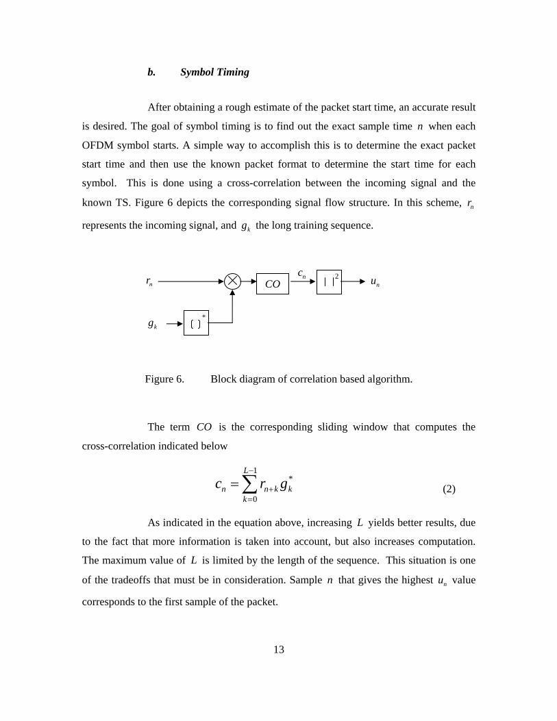
b. Symbol Timing
After obtaining a rough estimate of the packet start time, an accurate result
is desired. The goal of symbol timing is to find out the exact sample time n when each
OFDM symbol starts. A simple way to accomplish this is to determine the exact packet
start time and then use the known packet format to determine the start time for each
symbol. This is done using a cross-correlation between the incoming signal and the
known TS. Figure 6 depicts the corresponding signal flow structure. In this scheme, nr
represents the incoming signal, and kg the long training sequence.
Figure 6. Block diagram of correlation based algorithm.
The term CO is the corresponding sliding window that computes the
cross-correlation indicated below
1*
0
L
n n k kk
c r g−
+=
= ∑ (2)
As indicated in the equation above, increasing L yields better results, due
to the fact that more information is taken into account, but also increases computation.
The maximum value of L is limited by the length of the sequence. This situation is one
of the tradeoffs that must be in consideration. Sample n that gives the highest nu value
corresponds to the first sample of the packet.
nc nu 2
nr CO
kg *
14
c. Frequency Synchronization
As mentioned in [15], there are three types of algorithms for solving
frequency synchronization
• Data-aided algorithms,
• Nondata-aided algorithms, and
• Cyclic prefix based algorithms.
The best of the algorithm types suited for WLANs is the Data-aided type,
where the known training sequences permit us to obtain the frequency offset before the
start of the packet’s information payload.
Data-aided algorithms can be applied either in the time or frequency
domain, although the former is recommended, since computing the DFT of the symbols
increases computation without any advantage over the time domain approach.
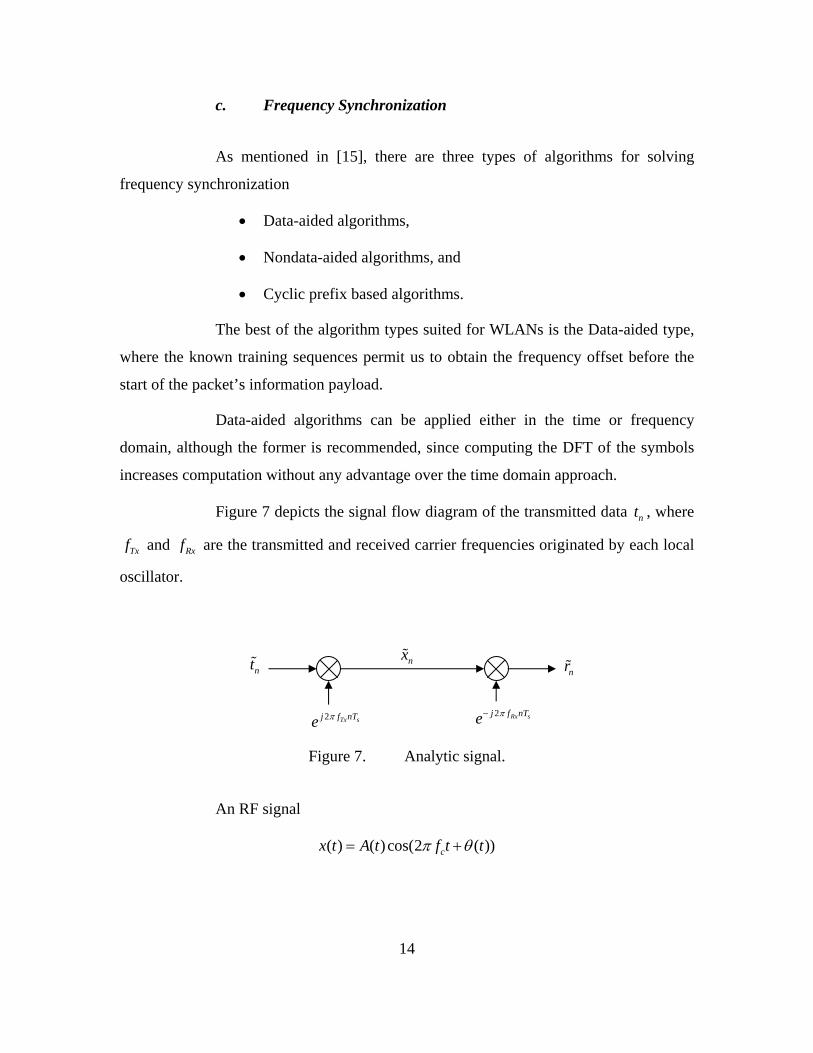
Figure 7 depicts the signal flow diagram of the transmitted data nt , where
Txf and Rxf are the transmitted and received carrier frequencies originated by each local
oscillator.
Figure 7. Analytic signal.
An RF signal
( ) ( ) cos(2 ( ))cx t A t f t tπ θ= +
nx nt
2 Tx sj f nTe π 2 Rx sj f nTe π−
nr
15
can be represented by its complex analytic signal [2 ( )]( ) ( ) cj f t tx t A t e π θ+=
Therefore the analytic transmitted signal from Figure 7 can be expressed as 2 tx sj f nT
n nx t e π= (3)
And the noiseless analytic received signal can be expressed as
2 Rx sj f nTn nr x e π=
2 sj f nTn nr t e π ∆= (4)
where Tx Rxf f f∆ = −
The frequency offset estimator is calculated after defining the following
intermediate variable [15]
1*
0
L
n n Dn
z r r−
+=
= ∑ (5)
In Equation (5) time delay D is the length of the training sequence, and L
is the length of the window used in the cross-correlation.
Substituting for nr in Equation (5) yields
122
0
s
Lj f DT
nn
z e tπ ∆
−−
=
= ∑ (6)
whereby the frequency offset is estimated as [15]
1 arg( ) 2 s
f zDTπ∆ = − (7)
16
d. Carrier Phase Tracking
Carrier phase tracking is an important task in a WLAN receiver. Its goal is
to eliminate the residual frequency error, remaining after applying the frequency
correction described in the last section. By enhancing frequency accuracy, constellation
rotation is avoided.
A data-aided based solution is used here also. The following type of
correction is performed for every symbol, using known information that is transmitted in
specific carriers, known as pilot sub-carriers or pilot tones. These pilots are going to be
affected by the channel, thus the phase difference between the transmitted and received
pilots needs to be calculated in order to perform the corresponding correction.
The sent pilot, ,s bP , and the received pilot, ,s bW , are related by
, ,s b s b bW P H= (8)
where s is the symbol index, b is the pilot index, and bH is the frequency response of
the pilot sub-carrier. However, the estimated channel frequency response ˆbH is not
perfect and therefore
ˆb b bH H α= (9)
where 2j sfs e δπα α= , and 2 sfδπ accounts for all the phase errors in ˆ
bH . Using the
estimated channel frequency response, we can calculate an estimated pilot
, ,ˆ ˆ
s b s b bW P H= (10)
We can determine the error in the phase of this estimate, and thereby the error in the
phase of our channel frequency response estimate by using the actual and estimated
received pilots
*, ,
1
ˆ ˆargB
s s b s bb
W Wθ=
⎛ ⎞= ⎜ ⎟
⎝ ⎠∑ (11)
17
*, ,
1
ˆarg ( )B
s b b s b bb
P H P H=
⎛ ⎞= ⎜ ⎟
⎝ ⎠∑
2 *,
1
ˆargB
s b b bb
P H H=
⎛ ⎞= ⎜ ⎟
⎝ ⎠∑
Since 2
,s bP is one, according to the standard, the error in the phase estimate is
*
1
ˆargB
b bb
H H=
⎛ ⎞= ⎜ ⎟
⎝ ⎠∑
*
1arg ( )
B
b bb
H H α=
⎛ ⎞= ⎜ ⎟
⎝ ⎠∑
2*
1arg
B
bb
Hα=
⎛ ⎞= ⎜ ⎟
⎝ ⎠∑
arg( )α= − (12)
After the packet is corrected for the estimated channel, it must be further rotated by
arg( )α− to correct for inaccurate phase measurement of bH .
e. Channel Estimation
A transmitted signal is affected by the channel and noise, as shown in the
frequency domain representation shown below
k k k kE H G W= + (13)
where 0,...., 1 and k N N= − is the index of the sub-carrier.
kE : Received Training Sequence (TS).
kG : Known transmitted TS.
kH : Channel frequency response.
kW : Noise.
18
A simple way to obtain the channel estimation is as follows
*ˆ .k k kH E G= (14)
Substituting (13) into (14) we obtain
( ) *ˆk k k k kH H G W G= + (15)
2 *k k k kH G W G= + (16)
The TS values are one or minus one; hence 2kG is equal to one and
*ˆk k k kH H W G= + (17)
Thus the channel estimation represents the effect of the channel and the noise over the
transmitted signal.
Using the average of two received TS, the computation of ˆkH can be
improved, because the noise terms will partially cancel while the channel term should be
essentially static.
*1 2ˆ2
k kk k
E EH G+⎛ ⎞= ⎜ ⎟⎝ ⎠
(18)
C. IEEE 802.11A
The 802.11a standard is one of a series of WLAN standards based on IEEE
802.11, which was released in 1997 and is well known as Wi-Fi. The original version
specifies a maximum data rate of 2 Mbps, using infrared signals or radio spread spectrum
at 2.4 GHz. The first amendment proposed was 802.11a, with a maximum data rate of 54
Mbps but operating in the 5 GHz band using Orthogonal Frequency Division
Multiplexing (OFDM). The second amendment proposed was 802.11b, with a maximum
data rate of 11 Mbps, operating at 2.4 GHz. The 802.11g amendment of this standard was
the third amendment of the physical layer. Using the 2.4 GHz band, 802.11g can achieve
data rates of 54 Mbps through OFDM and spread spectrum modulation.
19
This section describes some aspects of 802.11a, needed to understand the manner
in which the synchronization algorithms were implemented. The reader should recognize
that much of this work can be extended to 802.11g, with few changes.
1. Modulation Scheme
802.11a uses OFDM, a multi-carrier modulation scheme. The length of the IFFT
window is 64 points, where 48 sub-carriers carry user data, four are pilot tones, and the
remaining 12 are null tones. The null tones provide a guardband at both high and low
ends of the signal spectrum and eliminate the center sub-carrier, which suffers from self
mixing in some common hardware implementations. After applying the IFFT to generate
the time domain OFDM symbol to be transmitted, the last 16 time domain samples are
copied at the beginning of the symbol, yielding a total of 80 time samples per OFDM
symbol.
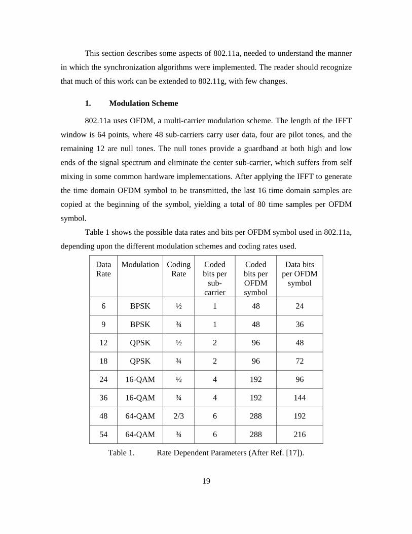
Table 1 shows the possible data rates and bits per OFDM symbol used in 802.11a,
depending upon the different modulation schemes and coding rates used.
Data Rate
Modulation Coding Rate
Coded bits per
sub-carrier
Coded bits per OFDM symbol
Data bits per OFDM
symbol
6 BPSK ½ 1 48 24
9 BPSK ¾ 1 48 36
12 QPSK ½ 2 96 48
18 QPSK ¾ 2 96 72
24 16-QAM ½ 4 192 96
36 16-QAM ¾ 4 192 144
48 64-QAM 2/3 6 288 192
54 64-QAM ¾ 6 288 216
Table 1. Rate Dependent Parameters (After Ref. [17]).
20
2. Packet Structure
Part 11 of the 802.11 standard [17], particularly the high-speed Physical layer
(PHY) in the 5 GHz Band specification, describes the PHY and Medium Access Control
(MAC) structure for 802.11a.
a. PHY for OFDM System Description
In order to send an 802.11a frame with minimum dependence on the PHY,
the PHY Layer Convergence Procedure (PLCP) is defined, which adds some fields
previously by the MAC layer.
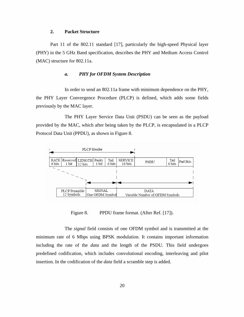
The PHY Layer Service Data Unit (PSDU) can be seen as the payload
provided by the MAC, which after being taken by the PLCP, is encapsulated in a PLCP
Protocol Data Unit (PPDU), as shown in Figure 8.
Figure 8. PPDU frame format. (After Ref. [17]).
The signal field consists of one OFDM symbol and is transmitted at the
minimum rate of 6 Mbps using BPSK modulation. It contains important information
including the rate of the data and the length of the PSDU. This field undergoes
predefined codification, which includes convolutional encoding, interleaving and pilot
insertion. In the codification of the data field a scramble step is added.
21
b. OFDM Specific Service Parameters
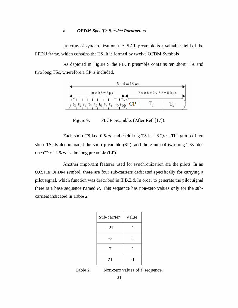
In terms of synchronization, the PLCP preamble is a valuable field of the
PPDU frame, which contains the TS. It is formed by twelve OFDM Symbols
As depicted in Figure 9 the PLCP preamble contains ten short TSs and
two long TSs, wherefore a CP is included.
Figure 9. PLCP preamble. (After Ref. [17]).
Each short TS last 0.8 sµ and each long TS last 3.2 sµ . The group of ten
short TSs is denominated the short preamble (SP), and the group of two long TSs plus
one CP of 1.6 sµ is the long preamble (LP).
Another important features used for synchronization are the pilots. In an
802.11a OFDM symbol, there are four sub-carriers dedicated specifically for carrying a
pilot signal, which function was described in II.B.2.d. In order to generate the pilot signal
there is a base sequence named P. This sequence has non-zero values only for the sub-
carriers indicated in Table 2.
Sub-carrier Value
-21 1
-7 1
7 1
21 -1
Table 2. Non-zero values of P sequence.
22
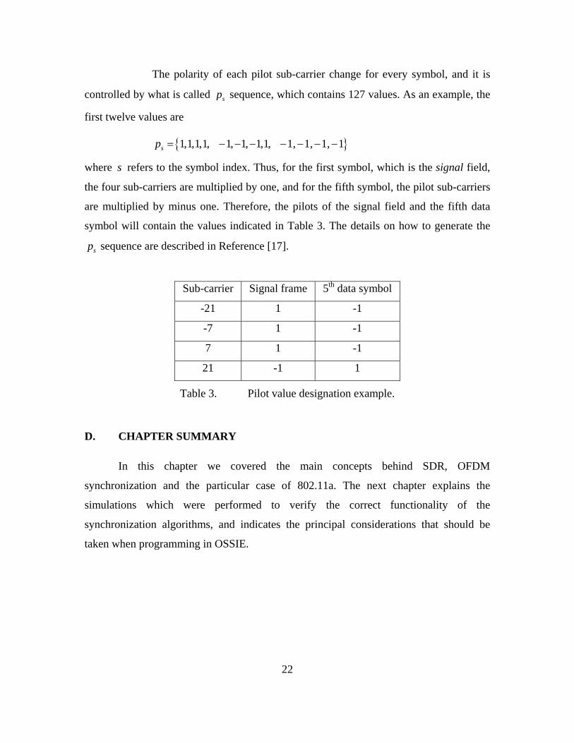
The polarity of each pilot sub-carrier change for every symbol, and it is
controlled by what is called sp sequence, which contains 127 values. As an example, the
first twelve values are
{ }1,1,1,1, 1, 1, 1,1, 1, 1, 1, 1sp = − − − − − − −
where s refers to the symbol index. Thus, for the first symbol, which is the signal field,
the four sub-carriers are multiplied by one, and for the fifth symbol, the pilot sub-carriers
are multiplied by minus one. Therefore, the pilots of the signal field and the fifth data
symbol will contain the values indicated in Table 3. The details on how to generate the
sp sequence are described in Reference [17].
Sub-carrier Signal frame 5th data symbol
-21 1 -1
-7 1 -1
7 1 -1
21 -1 1
Table 3. Pilot value designation example.
D. CHAPTER SUMMARY
In this chapter we covered the main concepts behind SDR, OFDM
synchronization and the particular case of 802.11a. The next chapter explains the
simulations which were performed to verify the correct functionality of the
synchronization algorithms, and indicates the principal considerations that should be
taken when programming in OSSIE.
23
III. SIMULATIONS AND DESIGN
A. MATLAB SIMULATION
The first step before developing the application was the verification of the
corresponding algorithms, which are involved in the synchronization process. For this
purpose, the software Matlab was chosen, since many required functions are already
developed and the vector and matrix oriented mathematics, make this software ideal for
simulations. Additionally, Matlab has a very good debugging tool, which helps to reduce
the time spent in finding errors.
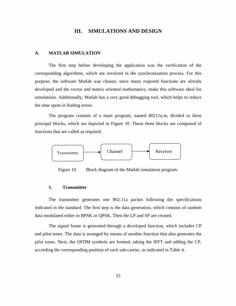
The program consists of a main program, named 80211a.m, divided in three
principal blocks, which are depicted in Figure 10. These three blocks are composed of
functions that are called as required.
Figure 10. Block diagram of the Matlab simulation program.
1. Transmitter
The transmitter generates one 802.11a packet following the specifications
indicated in the standard. The first step is the data generation, which consists of random
data modulated either in BPSK or QPSK. Then the LP and SP are created.
The signal frame is generated through a developed function, which includes CP
and pilot tones. The data is arranged by means of another function that also generates the
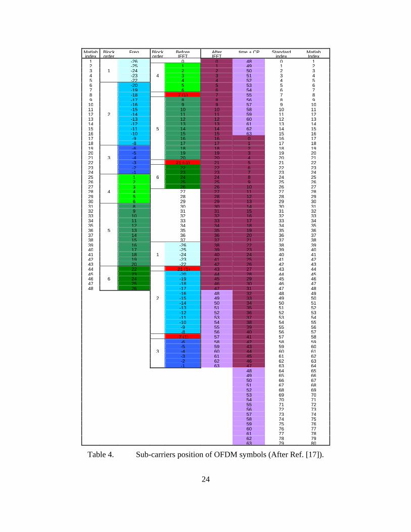
pilot tones. Next, the OFDM symbols are formed, taking the IFFT and adding the CP,
according the corresponding position of each sub-carrier, as indicated in Table 4.
Transmitter Receiver Channel
24
Matlab Block Freq Block Before After time + CP Standard Matlabindex order order IFFT IFFT index Index
1 -26 0 0 48 0 12 -25 1 1 49 1 23 1 -24 2 2 50 2 34 -23 4 3 3 51 3 45 -22 4 4 52 4 56 -20 5 5 53 5 67 -19 6 6 54 6 78 -18 7 (1) 7 55 7 89 -17 8 8 56 8 9
10 -16 9 9 57 9 1011 -15 10 10 58 10 1112 2 -14 11 11 59 11 1213 -13 12 12 60 12 1314 -12 13 13 61 13 1415 -11 5 14 14 62 14 1516 -10 15 15 63 15 1617 -9 16 16 0 16 1718 -8 17 17 1 17 1819 -6 18 18 2 18 1920 -5 19 19 3 19 2021 3 -4 20 20 4 20 2122 -3 21 (-1) 21 5 21 2223 -2 22 22 6 22 2324 -1 23 23 7 23 2425 1 6 24 24 8 24 2526 2 25 25 9 25 2627 3 26 26 10 26 2728 4 4 27 27 11 27 2829 5 28 28 12 28 2930 6 29 29 13 29 3031 8 30 30 14 30 3132 9 31 31 15 31 3233 10 32 32 16 32 3334 11 33 33 17 33 3435 12 34 34 18 34 3536 5 13 35 35 19 35 3637 14 36 36 20 36 3738 15 37 37 21 37 3839 16 -26 38 22 38 3940 17 -25 39 23 39 4041 18 1 -24 40 24 40 4142 19 -23 41 25 41 4243 20 -22 42 26 42 4344 22 -21 (1) 43 27 43 4445 23 -20 44 28 44 4546 6 24 -19 45 29 45 4647 25 -18 46 30 46 4748 26 -17 47 31 47 48
-16 48 32 48 492 -15 49 33 49 50
-14 50 34 50 51-13 51 35 51 52-12 52 36 52 53-11 53 37 53 54-10 54 38 54 55-9 55 39 55 56-8 56 40 56 57
-7 (1) 57 41 57 58-6 58 42 58 59-5 59 43 59 60
3 -4 60 44 60 61-3 61 45 61 62-2 62 46 62 63-1 63 47 63 64
48 64 6549 65 6650 66 6751 67 6852 68 6953 69 7054 70 7155 71 7256 72 7357 73 7458 74 7559 75 7660 76 7761 77 7862 78 7963 79 80
Table 4. Sub-carriers position of OFDM symbols (After Ref. [17]).

25
In Table 4, the carriers are divided into blocks, each with a particular number and
color, in order to show their correct position, before computing the IFFT. After the IFFT,
the last 16 values have a different color to illustrate that these are the CP and, as
explained before, added at the beginning of the symbol.
Finally the transmitter concatenates the preambles, signal frame and data frame,
in order to form the packet and upconvert it to an arbitrary carrier frequency.
The developed functions for this part of the program are indicated in Table 5.
Function Description Signal_frame() Generates the signal frame in the frequency domain. Data_frame() Generates the data frame in the frequency domain.
Table 5. List of functions defined in the Tx block.
2. Channel
This section of the simulation program is intended to affect the signal as in a
WLAN environment. To accomplish this, Additive White Gaussian Noise (AWGN) is
added to the signal, as well as a small frequency variation as might be caused by Doppler
shift, and multipath. These functions are indicated in Table 6.
Function Description Frequency_offset() Generates a frequency offset in the carrier frequency. AWGN() Add AWGN to the signal. Multipath() Includes more than one path to the transmission.
Table 6. List of functions defined in Channel block.
In order to simulate a multipath environment, the Multipath() function includes
the Matlab function rayleighchan(), where the time delay and the gain of the different
paths are defined.
26
3. Receiver
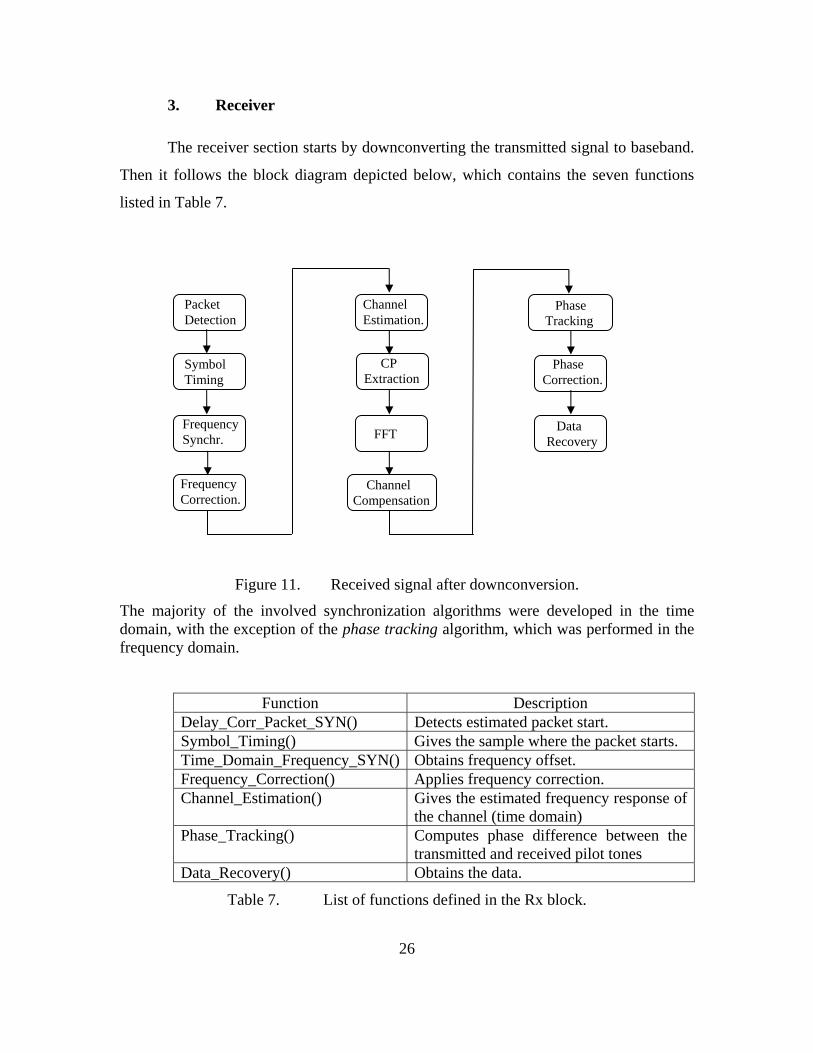
The receiver section starts by downconverting the transmitted signal to baseband.
Then it follows the block diagram depicted below, which contains the seven functions
listed in Table 7.
Figure 11. Received signal after downconversion.
The majority of the involved synchronization algorithms were developed in the time domain, with the exception of the phase tracking algorithm, which was performed in the frequency domain.
Function Description Delay_Corr_Packet_SYN() Detects estimated packet start. Symbol_Timing() Gives the sample where the packet starts. Time_Domain_Frequency_SYN() Obtains frequency offset. Frequency_Correction() Applies frequency correction. Channel_Estimation() Gives the estimated frequency response of
the channel (time domain) Phase_Tracking() Computes phase difference between the
transmitted and received pilot tones Data_Recovery() Obtains the data.
Table 7. List of functions defined in the Rx block.
Data Recovery
Phase Correction.
Phase Tracking
Channel Compensation
CP Extraction
Channel Estimation.
Frequency Correction.
Frequency Synchr.
Packet Detection
Symbol Timing
FFT

27
The Delay_Corr_Packet_SYN() function performs the algorithm discussed in
II.B.2.a. This function needs a definition regarding the value of the threshold that
indicates that a valid packet is coming. Furthermore, this setting is not enough, since an
isolated peak caused by noise could cross the threshold. Thus, the decision must be made
considering more than one cross-threshold value. For this simulation 20 cross-threshold
value in a row gave a reliable result, empirically based. It is expected that this value
depends on noise environment.
The Time_Domain_Frequency_SYN() and Frequency_Correction() functions are
used sequentially more than once, in order to determine the best performance using either
the SP or LP. These functions accomplish the algorithms indicated in II.B.2.c.
4. Results
In order to prove the algorithms, the signal was subjected to different types of
distortions.
a. AWGN
The noise we chose is such that 0/bE N is 10 dB. The noisy signal is
y x sig N= + i (19)
where: x : original signal.
y : noisy signal.
N : noise of zero mean and unit variance.
2
0
( )/b d
mean x WsigE N R
=⋅i (20)
In (20) the bandwidth W is a fixed value of 312.5 kHz, regardless the modulation
scheme used. The data rate dR is set to 6 Mbps for the BPSK case, and 12 Mbps for
QPSK.

28
b. Frequency Offset
As described in [15], the applied algorithm allows a limited frequency
error, defined by
12 s
fDT∆ ≤ (21)
where D is the length of the TS.
The expected maximum frequency offset using the SP is 625 kHz, and
using the LP is 156.25 kHz. On the other hand, the maximum error allowed by the
standard is 212 kHz.
Different values of frequency error were applied, verifying the last
paragraph, and the algorithm’s functionality. Although use of LP can correct a smaller
range of offset frequencies, it gives a more accurate result. Thus, a recommended
alternative [15] is to calculate a coarse frequency offset with the SP (which has a better
operational range), correct the LP, and finally estimate a fine frequency offset using the
LP. The next example consists of computing the frequency offset of a BPSK signal,
already affected by noise.
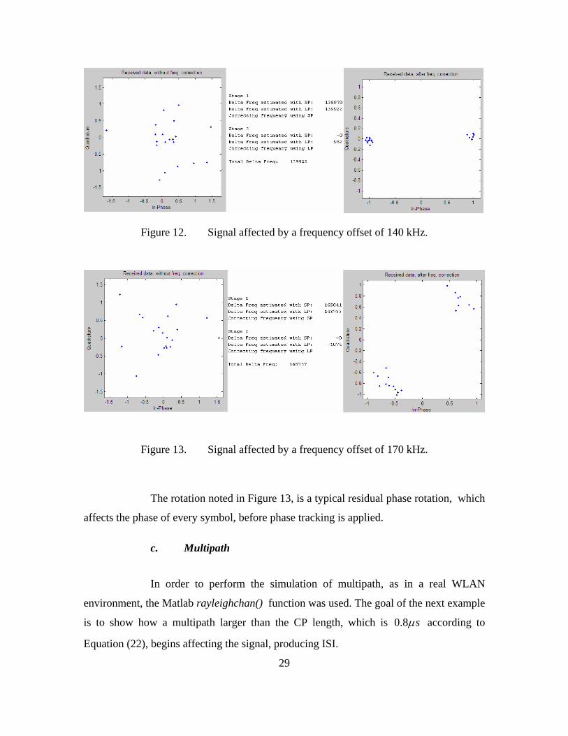
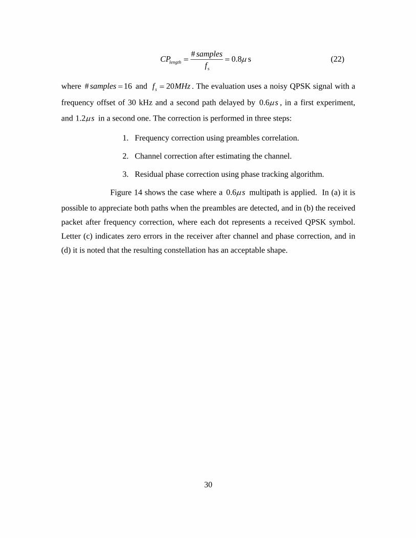
Figure 12 depicts the case where a 140 kHz offset is applied. It is noted
that the second stage is not needed, since the LP method computes an accurate offset in
the first stage. In Figure 13, an applied 170 kHz offset does not allow the LP method to
compute a reliable offset in the first stage, thus a frequency correction is applied using the
coarse result obtained by the SP method. Now, a second stage using the result utilizing
the LP, can enhance the accuracy of the frequency offset.
29
Figure 12. Signal affected by a frequency offset of 140 kHz.
Figure 13. Signal affected by a frequency offset of 170 kHz.
The rotation noted in Figure 13, is a typical residual phase rotation, which
affects the phase of every symbol, before phase tracking is applied.
c. Multipath
In order to perform the simulation of multipath, as in a real WLAN
environment, the Matlab rayleighchan() function was used. The goal of the next example
is to show how a multipath larger than the CP length, which is 0.8 sµ according to
Equation (22), begins affecting the signal, producing ISI.
30
# 0.8 slengths
samplesCPf
µ= = (22)
where # 16samples = and 20sf MHz= . The evaluation uses a noisy QPSK signal with a
frequency offset of 30 kHz and a second path delayed by 0.6 sµ , in a first experiment,
and 1.2 sµ in a second one. The correction is performed in three steps:
1. Frequency correction using preambles correlation.
2. Channel correction after estimating the channel.
3. Residual phase correction using phase tracking algorithm.
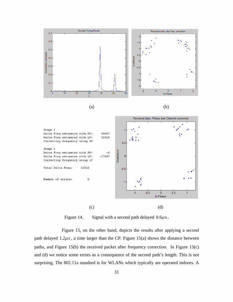
Figure 14 shows the case where a 0.6 sµ multipath is applied. In (a) it is
possible to appreciate both paths when the preambles are detected, and in (b) the received
packet after frequency correction, where each dot represents a received QPSK symbol.
Letter (c) indicates zero errors in the receiver after channel and phase correction, and in
(d) it is noted that the resulting constellation has an acceptable shape.
31
(a) (b)
(c) (d)
Figure 14. Signal with a second path delayed 0.6 sµ .
Figure 15, on the other hand, depicts the results after applying a second
path delayed 1.2 sµ , a time larger than the CP. Figure 15(a) shows the distance between
paths, and Figure 15(b) the received packet after frequency correction. In Figure 15(c)
and (d) we notice some errors as a consequence of the second path’s length. This is not
surprising. The 802.11a standard is for WLANs which typically are operated indoors. A
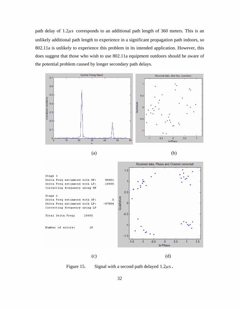
32
path delay of 1.2 sµ corresponds to an additional path length of 360 meters. This is an
unlikely additional path length to experience in a significant propagation path indoors, so
802.11a is unlikely to experience this problem in its intended application. However, this
does suggest that those who wish to use 802.11a equipment outdoors should be aware of
the potential problem caused by longer secondary path delays.
(a) (b)
(c) (d)
Figure 15. Signal with a second path delayed 1.2 sµ .
33
B. OSSIE DESIGN
1. Design Considerations
As mentioned before, OSSIE enables the engineer to develop waveforms and
components, by using the OSSIE Waveform Developer (OWD). In order to create a
waveform, it is necessary to have available the required components. Some helpful
features of OWD include the capability to write and edit components, manage ports and
include properties.
a. Components
An important characteristic of the OWD is the automatic code that is
generated when a component is created. This not only allows the component to interact
with the rest of the files needed to be installed on a system, but permits the programmer
to focus just on the communication task the component should achieve.
After creating a component, the second step is to write the code for a
specific task. For this purposes, the commented line “// insert code here to do work”,
within the function process_data(), indicates where to locate the code.
The code written by the programmer is located inside a while() loop,
which is permanently executed while the component is active. This is an important point
under consideration when designing components. Usually the loop starts with a specific
function, which allows reading the incoming buffer, getting the data from the previous
component. The loop ends by delivering the processed data to the next component and
erasing the incoming buffer, leaving it ready to read again.
b. Ports
With the release of OSSIE version 0.6.1, the management of ports has
been simplified. There are two types of ports: uses and provides. The first one refers to
the port that sends data out of the component and into the core framework (the core
framework uses the data); the latter, to the component port that receives data from
34
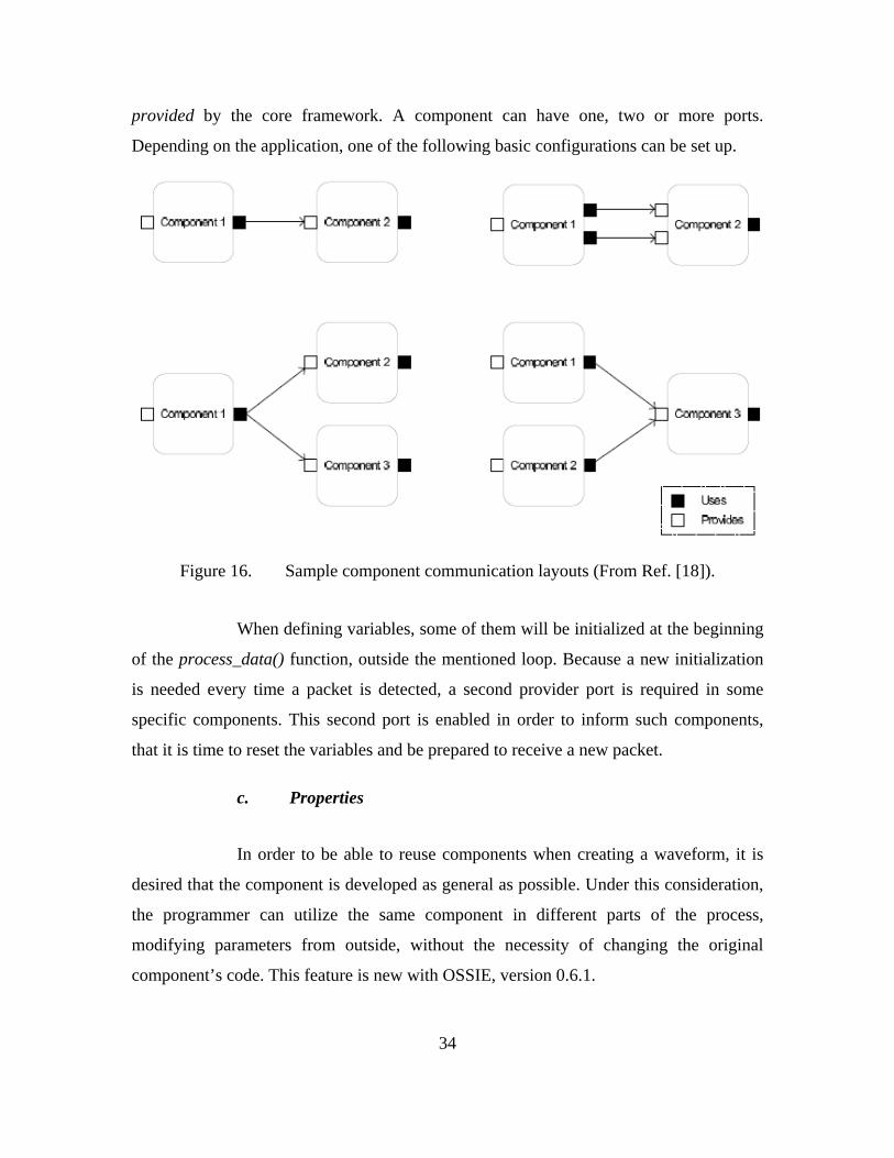
provided by the core framework. A component can have one, two or more ports.
Depending on the application, one of the following basic configurations can be set up.
Figure 16. Sample component communication layouts (From Ref. [18]).
When defining variables, some of them will be initialized at the beginning
of the process_data() function, outside the mentioned loop. Because a new initialization
is needed every time a packet is detected, a second provider port is required in some
specific components. This second port is enabled in order to inform such components,
that it is time to reset the variables and be prepared to receive a new packet.
c. Properties
In order to be able to reuse components when creating a waveform, it is
desired that the component is developed as general as possible. Under this consideration,
the programmer can utilize the same component in different parts of the process,
modifying parameters from outside, without the necessity of changing the original
component’s code. This feature is new with OSSIE, version 0.6.1.
35
2. Synchronization Components Structure
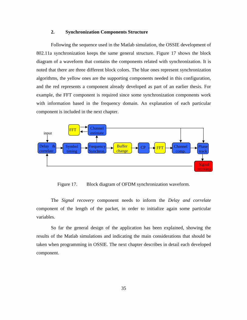
Following the sequence used in the Matlab simulation, the OSSIE development of
802.11a synchronization keeps the same general structure. Figure 17 shows the block
diagram of a waveform that contains the components related with synchronization. It is
noted that there are three different block colors. The blue ones represent synchronization
algorithms, the yellow ones are the supporting components needed in this configuration,
and the red represents a component already developed as part of an earlier thesis. For
example, the FFT component is required since some synchronization components work
with information based in the frequency domain. An explanation of each particular
component is included in the next chapter.
Figure 17. Block diagram of OFDM synchronization waveform.
The Signal recovery component needs to inform the Delay and correlate
component of the length of the packet, in order to initialize again some particular
variables.
So far the general design of the application has been explained, showing the
results of the Matlab simulations and indicating the main considerations that should be
taken when programming in OSSIE. The next chapter describes in detail each developed
component.
Frequency Synchron.
Channel estimate
FFT
Buffer change
CP FFT Delay & correlate
input
Symbol timing
Channel comp.
Phase track
Signal recovery

36
THIS PAGE INTENTIONALLY LEFT BLANK
37
IV. OSSIE COMPONENT DEVELOPMENT
A. SYNCHRONIZATION COMPONENT DEVELOPMENT
This section describes the development of each component needed in the synchronization stage of the 802.11a receiver.
1. Component Development Using OSSIE
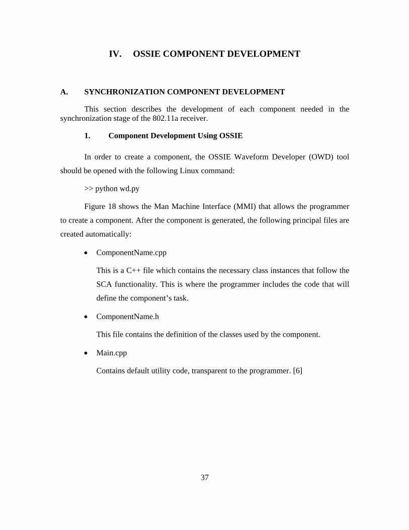
In order to create a component, the OSSIE Waveform Developer (OWD) tool
should be opened with the following Linux command:
>> python wd.py
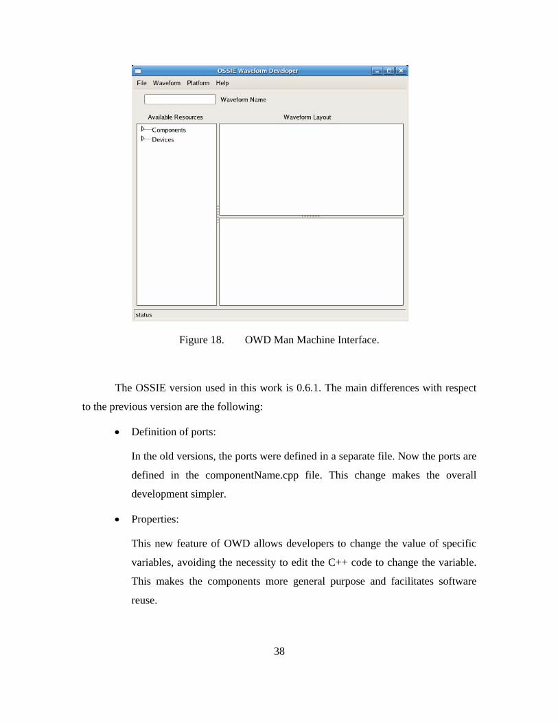
Figure 18 shows the Man Machine Interface (MMI) that allows the programmer
to create a component. After the component is generated, the following principal files are
created automatically:
• ComponentName.cpp
This is a C++ file which contains the necessary class instances that follow the
SCA functionality. This is where the programmer includes the code that will
define the component’s task.
• ComponentName.h
This file contains the definition of the classes used by the component.
• Main.cpp
Contains default utility code, transparent to the programmer. [6]
38
Figure 18. OWD Man Machine Interface.
The OSSIE version used in this work is 0.6.1. The main differences with respect
to the previous version are the following:
• Definition of ports:
In the old versions, the ports were defined in a separate file. Now the ports are
defined in the componentName.cpp file. This change makes the overall
development simpler.
• Properties:
This new feature of OWD allows developers to change the value of specific
variables, avoiding the necessity to edit the C++ code to change the variable.
This makes the components more general purpose and facilitates software
reuse.
39
2. Synchronization Stage Components
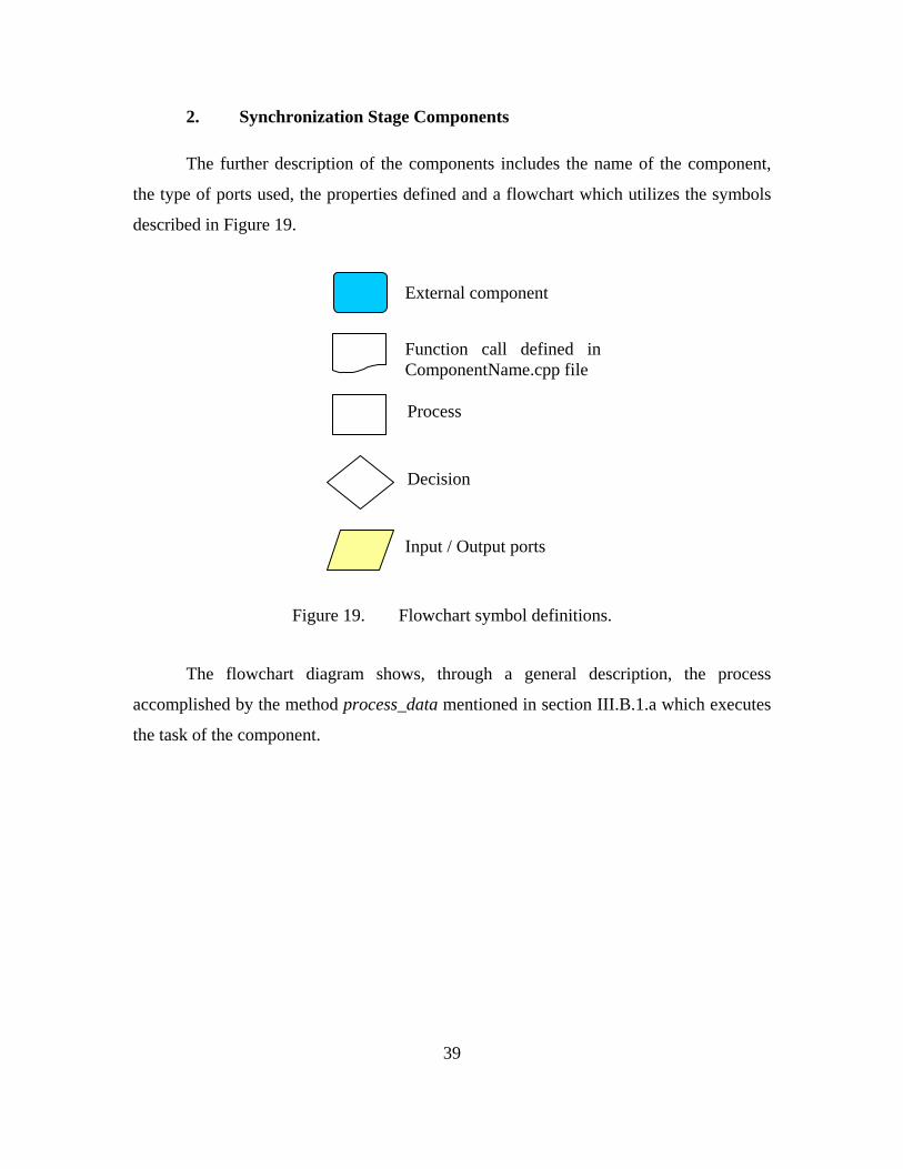
The further description of the components includes the name of the component,
the type of ports used, the properties defined and a flowchart which utilizes the symbols
described in Figure 19.
Figure 19. Flowchart symbol definitions.
The flowchart diagram shows, through a general description, the process
accomplished by the method process_data mentioned in section III.B.1.a which executes
the task of the component.
External component
Process
Decision
Input / Output ports
Function call defined in ComponentName.cpp file
40
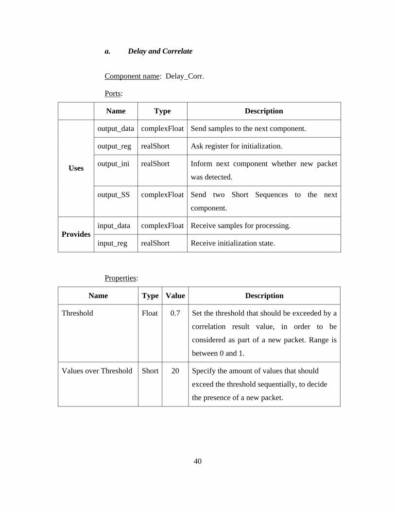
a. Delay and Correlate
Component name: Delay_Corr.
Ports:
Name Type Description
output_data complexFloat Send samples to the next component.
output_reg realShort Ask register for initialization.
output_ini realShort Inform next component whether new packet
was detected. Uses
output_SS complexFloat Send two Short Sequences to the next
component.
input_data complexFloat Receive samples for processing. Provides
input_reg realShort Receive initialization state.
Properties:
Name Type Value Description
Threshold Float 0.7 Set the threshold that should be exceeded by a
correlation result value, in order to be
considered as part of a new packet. Range is
between 0 and 1.
Values over Threshold Short 20 Specify the amount of values that should
exceed the threshold sequentially, to decide
the presence of a new packet.
41
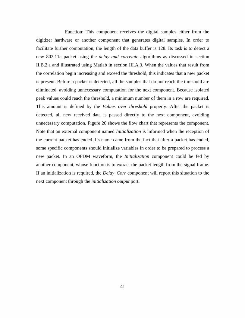
Function: This component receives the digital samples either from the
digitizer hardware or another component that generates digital samples. In order to
facilitate further computation, the length of the data buffer is 128. Its task is to detect a
new 802.11a packet using the delay and correlate algorithms as discussed in section
II.B.2.a and illustrated using Matlab in section III.A.3. When the values that result from
the correlation begin increasing and exceed the threshold, this indicates that a new packet
is present. Before a packet is detected, all the samples that do not reach the threshold are
eliminated, avoiding unnecessary computation for the next component. Because isolated
peak values could reach the threshold, a minimum number of them in a row are required.
This amount is defined by the Values over threshold property. After the packet is
detected, all new received data is passed directly to the next component, avoiding
unnecessary computation. Figure 20 shows the flow chart that represents the component.
Note that an external component named Initialization is informed when the reception of
the current packet has ended. Its name came from the fact that after a packet has ended,
some specific components should initialize variables in order to be prepared to process a
new packet. In an OFDM waveform, the Initialization component could be fed by
another component, whose function is to extract the packet length from the signal frame.
If an initialization is required, the Delay_Corr component will report this situation to the
next component through the initialization output port.
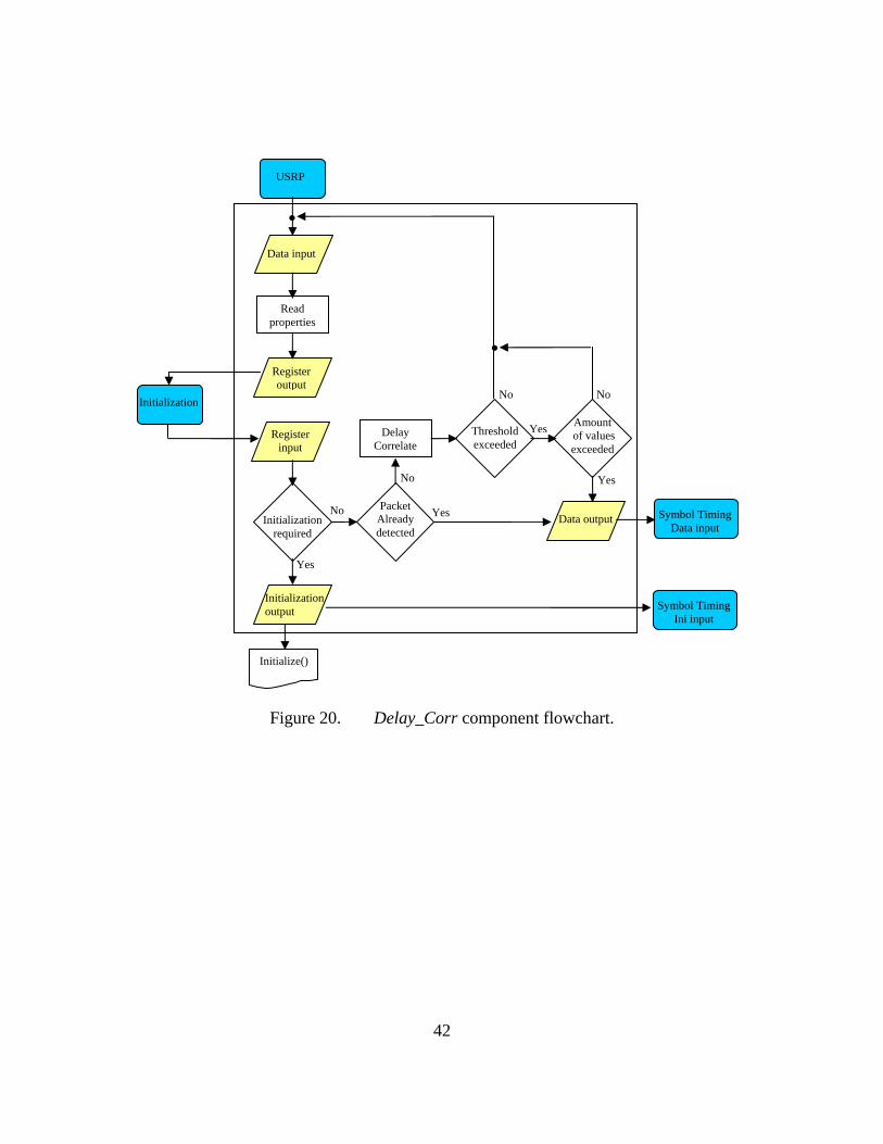
42
Figure 20. Delay_Corr component flowchart.
Data input
Read properties
Register output
Register input
Initialization required
Delay Correlate
Threshold exceeded
Amount of values exceeded
Data output
Initialization output
Initialize()
Packet Already detected
Symbol Timing Data input
Yes
No
Yes
Yes
Yes
No No
No
.
USRP
.
Symbol Timing Ini input
Initialization
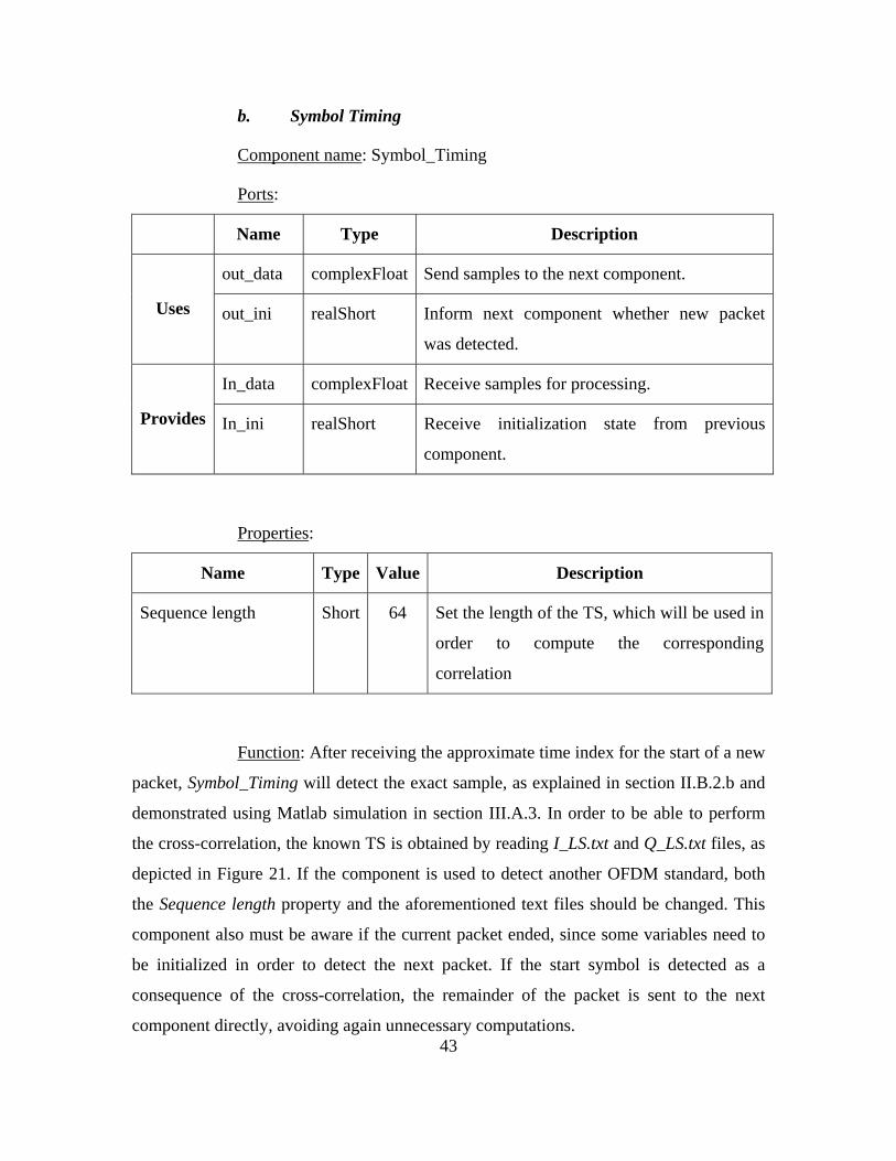
43
b. Symbol Timing
Component name: Symbol_Timing
Ports:
Name Type Description
out_data complexFloat Send samples to the next component.
Uses out_ini realShort Inform next component whether new packet
was detected.
In_data complexFloat Receive samples for processing.
Provides In_ini realShort Receive initialization state from previous
component.
Properties:
Name Type Value Description
Sequence length Short 64 Set the length of the TS, which will be used in
order to compute the corresponding
correlation
Function: After receiving the approximate time index for the start of a new
packet, Symbol_Timing will detect the exact sample, as explained in section II.B.2.b and
demonstrated using Matlab simulation in section III.A.3. In order to be able to perform
the cross-correlation, the known TS is obtained by reading I_LS.txt and Q_LS.txt files, as
depicted in Figure 21. If the component is used to detect another OFDM standard, both
the Sequence length property and the aforementioned text files should be changed. This
component also must be aware if the current packet ended, since some variables need to
be initialized in order to detect the next packet. If the start symbol is detected as a
consequence of the cross-correlation, the remainder of the packet is sent to the next
component directly, avoiding again unnecessary computations.
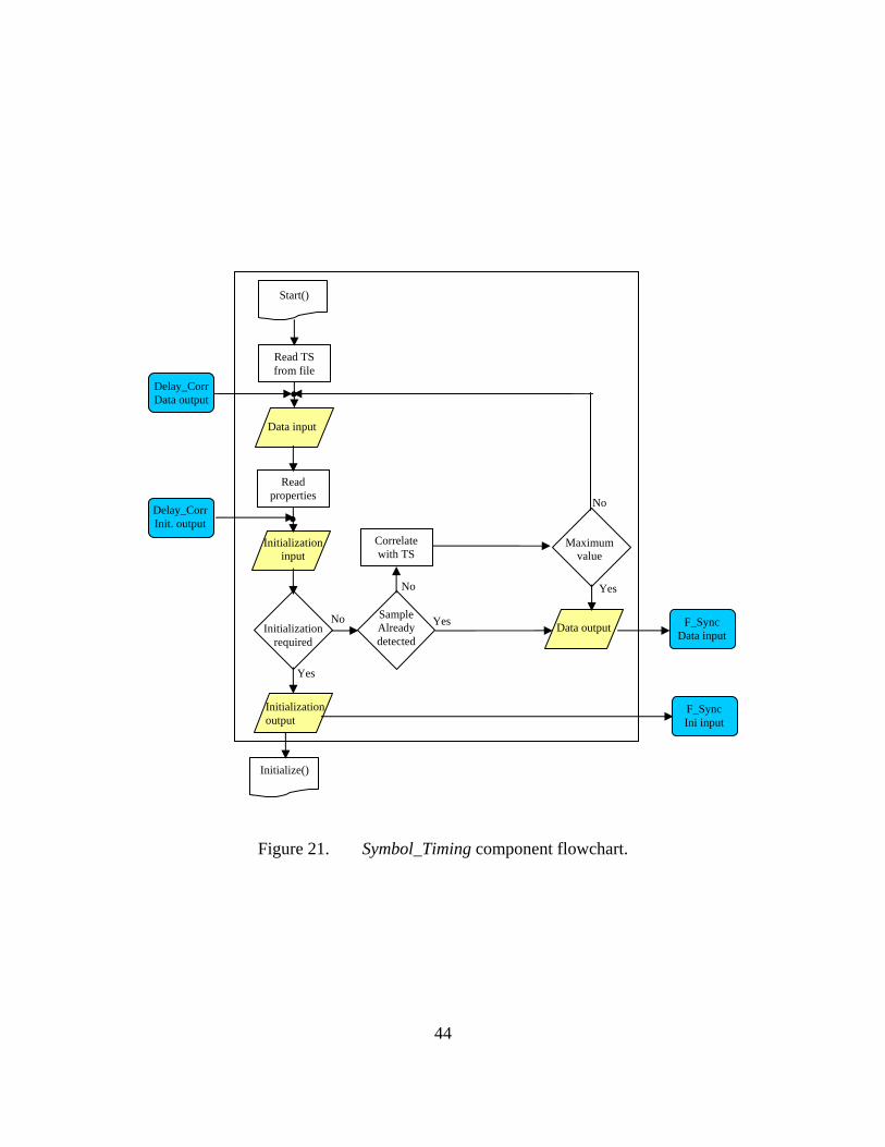
44
Figure 21. Symbol_Timing component flowchart.
Data input
Read properties
Initialization input
Initialization required
Correlate with TS
Maximum value
Data output
Initialization output
Initialize()
Sample Already detected
F_Sync Data input
Yes
No
Yes
Yes
No
No
Delay_Corr Data output
Start()
Read TS from file .
. Delay_Corr Init. output
F_Sync Ini input
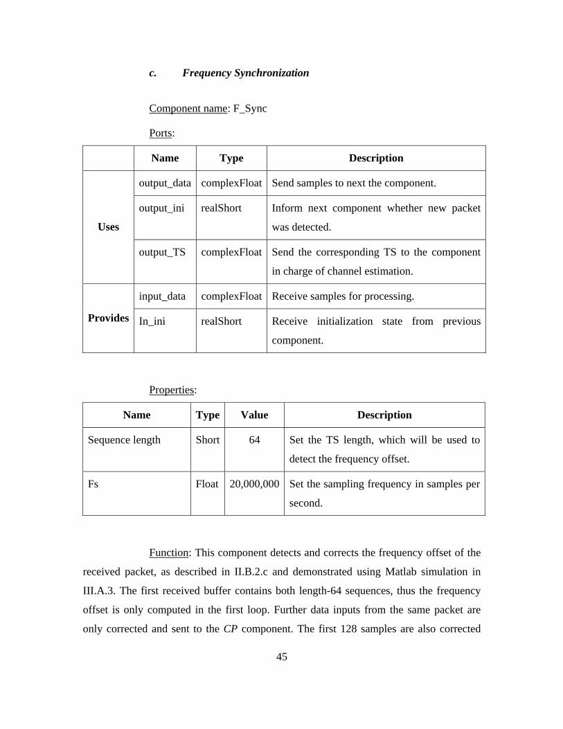
45
c. Frequency Synchronization
Component name: F_Sync
Ports:
Name Type Description
output_data complexFloat Send samples to next the component.
output_ini realShort Inform next component whether new packet
was detected. Uses
output_TS complexFloat Send the corresponding TS to the component
in charge of channel estimation.
input_data complexFloat Receive samples for processing.
Provides In_ini realShort Receive initialization state from previous
component.
Properties:
Name Type Value Description
Sequence length Short 64 Set the TS length, which will be used to
detect the frequency offset.
Fs Float 20,000,000 Set the sampling frequency in samples per
second.
Function: This component detects and corrects the frequency offset of the
received packet, as described in II.B.2.c and demonstrated using Matlab simulation in
III.A.3. The first received buffer contains both length-64 sequences, thus the frequency
offset is only computed in the first loop. Further data inputs from the same packet are
only corrected and sent to the CP component. The first 128 samples are also corrected
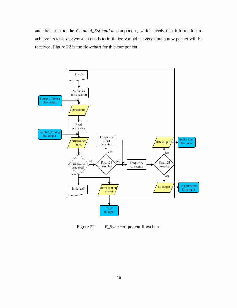
46
and then sent to the Channel_Estimation component, which needs that information to
achieve its task. F_Sync also needs to initialize variables every time a new packet will be
received. Figure 22 is the flowchart for this component.
Figure 22. F_Sync component flowchart.
Data input
Read properties
Initialization input
Initialization required
Frequency offset
detection Data output
Initialize()
First 128 samples
Buffer Size Data input
Yes
No
Yes
No
Symbol_Timing Data output
Start()
Variables initialization .
.
Frequency correction .
Symbol_Timing Ini. output
LP output
First 128 samples
No
Yes
Initialization output
.
Ch_C Ini input
Ch Estimation Data input
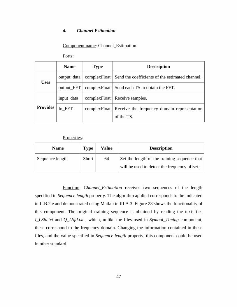
47
d. Channel Estimation
Component name: Channel_Estimation
Ports:
Name Type Description
output_data complexFloat Send the coefficients of the estimated channel. Uses
output_FFT complexFloat Send each TS to obtain the FFT.
input_data complexFloat Receive samples.
Provides In_FFT complexFloat Receive the frequency domain representation
of the TS.
Properties:
Name Type Value Description
Sequence length Short 64 Set the length of the training sequence that
will be used to detect the frequency offset.
Function: Channel_Estimation receives two sequences of the length
specified in Sequence length property. The algorithm applied corresponds to the indicated
in II.B.2.e and demonstrated using Matlab in III.A.3. Figure 23 shows the functionality of
this component. The original training sequence is obtained by reading the text files
I_LSfd.txt and Q_LSfd.txt , which, unlike the files used in Symbol_Timing component,
these correspond to the frequency domain. Changing the information contained in these
files, and the value specified in Sequence length property, this component could be used
in other standard.
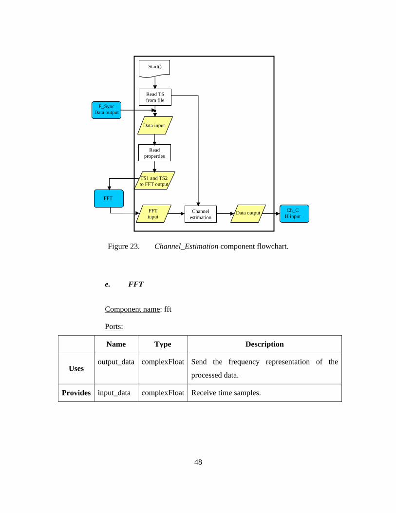
48
Figure 23. Channel_Estimation component flowchart.
e. FFT
Component name: fft
Ports:
Name Type Description
Uses output_data complexFloat Send the frequency representation of the
processed data.
Provides input_data complexFloat Receive time samples.
Data input
Read properties
TS1 and TS2 to FFT output
Data output Ch_C H input
Start()
Read TS from file .
Channel estimation
FFT
FFT input
F_Sync Data output

49
Properties:
Name Type Value Description
Length Short 64 Set the length of the FFT.
Function: This component utilizes the open source C++ library named fftw
[19] which contains the necessary functions for applying the FFT to the incoming signal.
The specific function that performs the FFT operation is fftwf_plan_dft_1d(), where two
arrays of the special type fftwf_complex are included. These arrays are named in and out.
The first carries the time samples to be processed and the latter the resulting frequency
samples. Other functions delete the variables and liberate the corresponding memory.
Figure 24 indicates the different steps executed by the FFT component.
Figure 24. FFT component flowchart.
Data input
Read properties
Data output Ch_C or Ch_Est Data input
Start()
Call fftw functions
.
FFT
Channel_Estimation or CP_Removal Data output
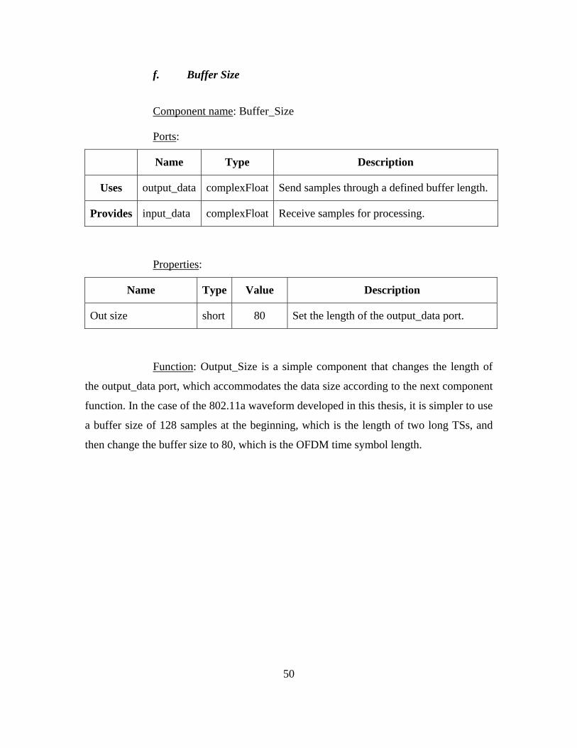
50
f. Buffer Size
Component name: Buffer_Size
Ports:
Name Type Description
Uses output_data complexFloat Send samples through a defined buffer length.
Provides input_data complexFloat Receive samples for processing.
Properties:
Name Type Value Description
Out size short 80 Set the length of the output_data port.
Function: Output_Size is a simple component that changes the length of
the output_data port, which accommodates the data size according to the next component
function. In the case of the 802.11a waveform developed in this thesis, it is simpler to use
a buffer size of 128 samples at the beginning, which is the length of two long TSs, and
then change the buffer size to 80, which is the OFDM time symbol length.
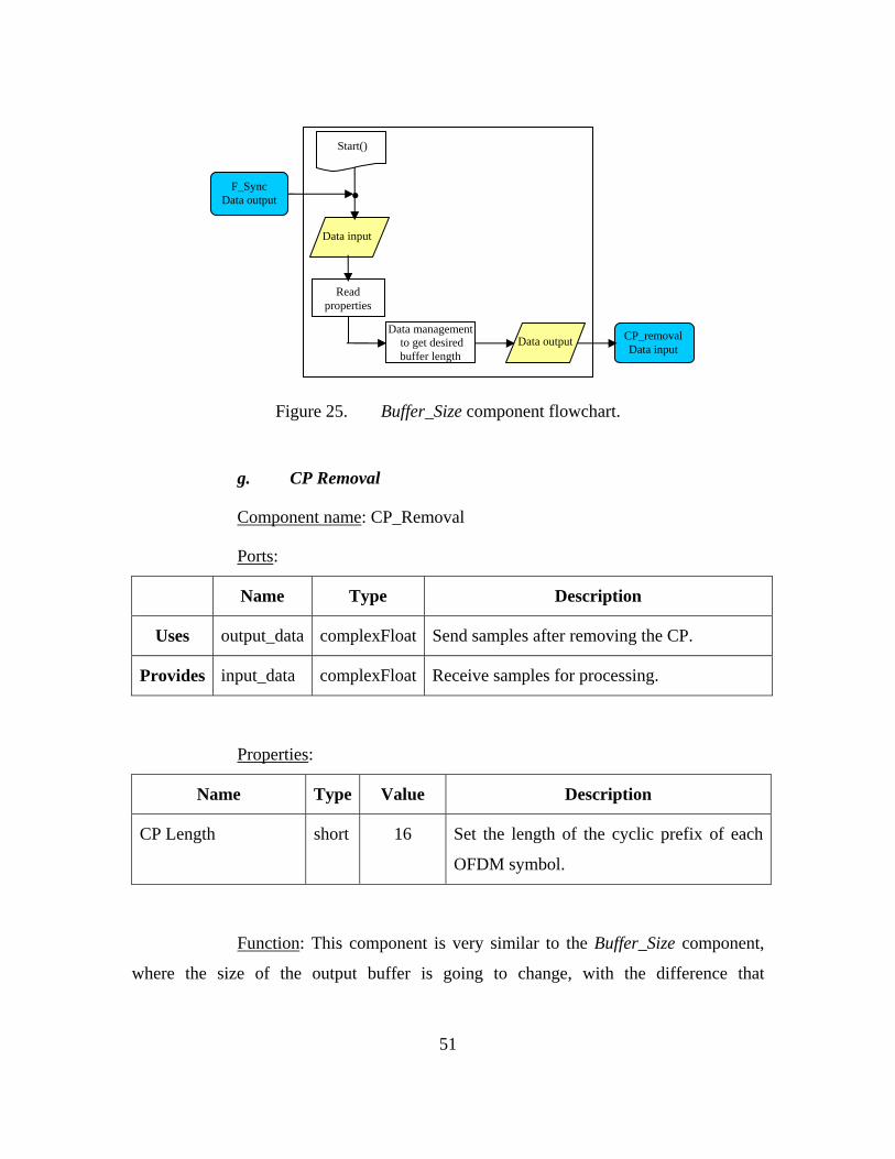
51
Figure 25. Buffer_Size component flowchart.
g. CP Removal
Component name: CP_Removal
Ports:
Name Type Description
Uses output_data complexFloat Send samples after removing the CP.
Provides input_data complexFloat Receive samples for processing.
Properties:
Name Type Value Description
CP Length short 16 Set the length of the cyclic prefix of each
OFDM symbol.
Function: This component is very similar to the Buffer_Size component,
where the size of the output buffer is going to change, with the difference that
Data input
Read properties
Data output CP_removal Data input
Start()
.
Data management to get desired buffer length
F_Sync Data output
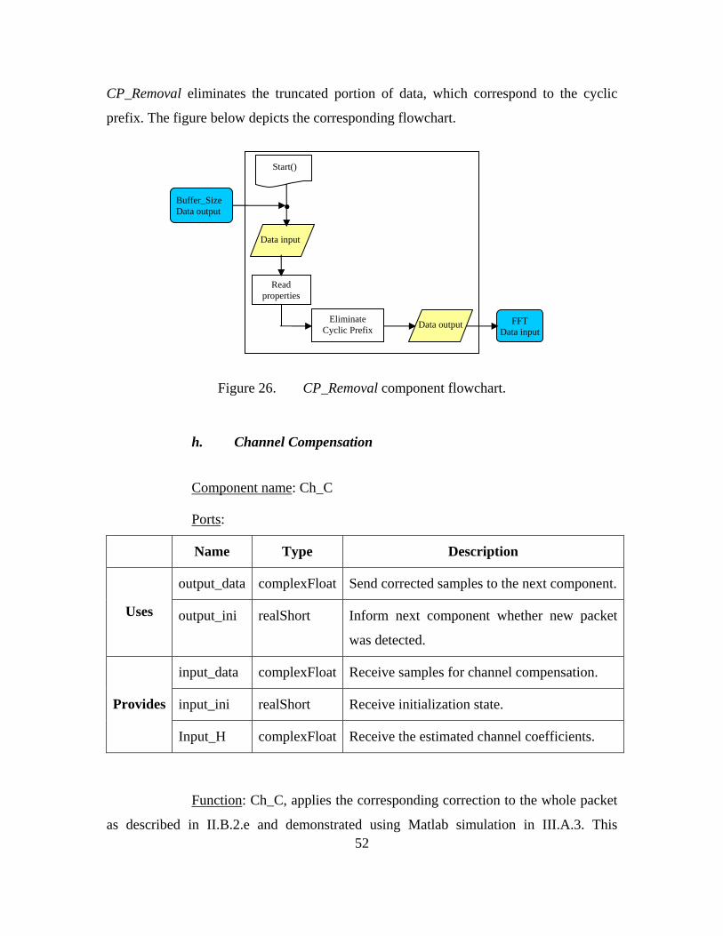
52
CP_Removal eliminates the truncated portion of data, which correspond to the cyclic
prefix. The figure below depicts the corresponding flowchart.
Figure 26. CP_Removal component flowchart.
h. Channel Compensation
Component name: Ch_C
Ports:
Name Type Description
output_data complexFloat Send corrected samples to the next component.
Uses output_ini realShort Inform next component whether new packet
was detected.
input_data complexFloat Receive samples for channel compensation.
input_ini realShort Receive initialization state. Provides
Input_H complexFloat Receive the estimated channel coefficients.
Function: Ch_C, applies the corresponding correction to the whole packet
as described in II.B.2.e and demonstrated using Matlab simulation in III.A.3. This
Data input
Read properties
Data output FFT Data input
Start()
.
Eliminate Cyclic Prefix
Buffer_Size Data output
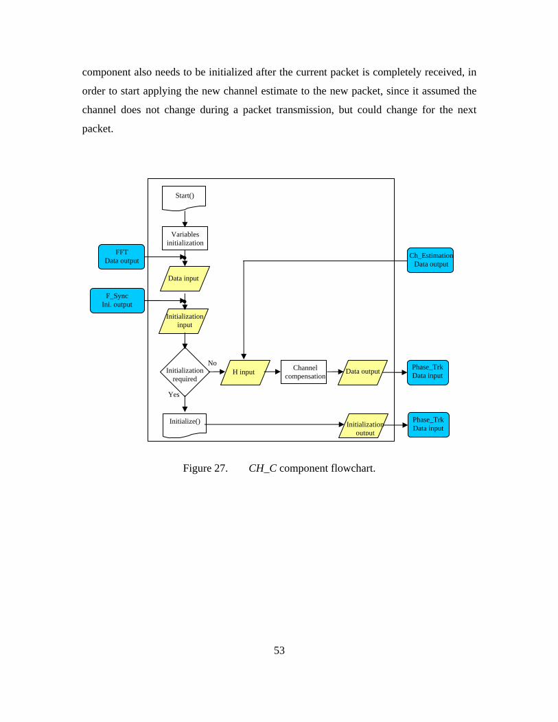
53
component also needs to be initialized after the current packet is completely received, in
order to start applying the new channel estimate to the new packet, since it assumed the
channel does not change during a packet transmission, but could change for the next
packet.
Figure 27. CH_C component flowchart.
Data input
Initialization input
Initialization required
Initialize()
Yes
No
FFT Data output
Start()
Variables initialization .
.
Channel compensation
F_Sync Ini. output
Data output Phase_Trk Data input
Initialization output
H input
Ch_Estimation Data output
Phase_Trk Data input
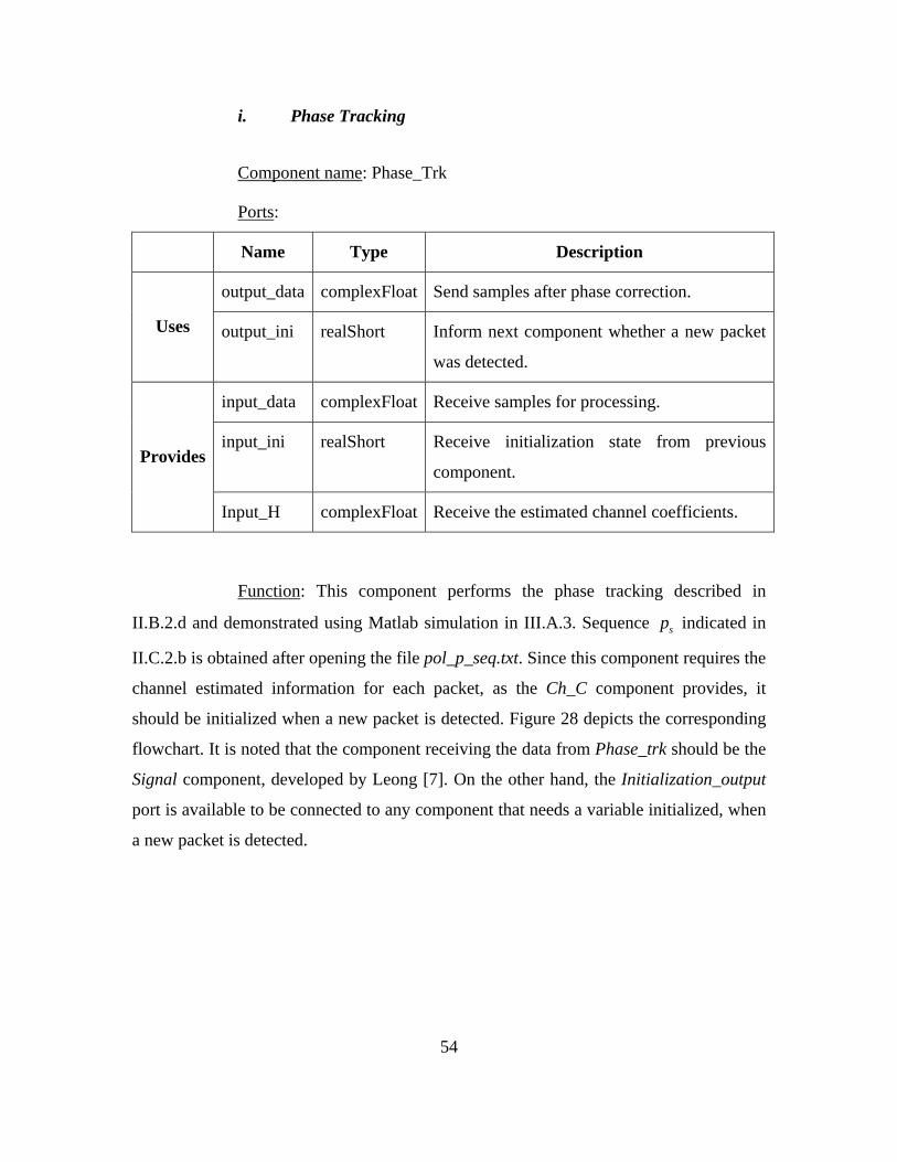
54
i. Phase Tracking
Component name: Phase_Trk
Ports:
Name Type Description
output_data complexFloat Send samples after phase correction.
Uses output_ini realShort Inform next component whether a new packet
was detected.
input_data complexFloat Receive samples for processing.
input_ini realShort Receive initialization state from previous
component. Provides
Input_H complexFloat Receive the estimated channel coefficients.
Function: This component performs the phase tracking described in
II.B.2.d and demonstrated using Matlab simulation in III.A.3. Sequence sp indicated in
II.C.2.b is obtained after opening the file pol_p_seq.txt. Since this component requires the
channel estimated information for each packet, as the Ch_C component provides, it
should be initialized when a new packet is detected. Figure 28 depicts the corresponding
flowchart. It is noted that the component receiving the data from Phase_trk should be the
Signal component, developed by Leong [7]. On the other hand, the Initialization_output
port is available to be connected to any component that needs a variable initialized, when
a new packet is detected.
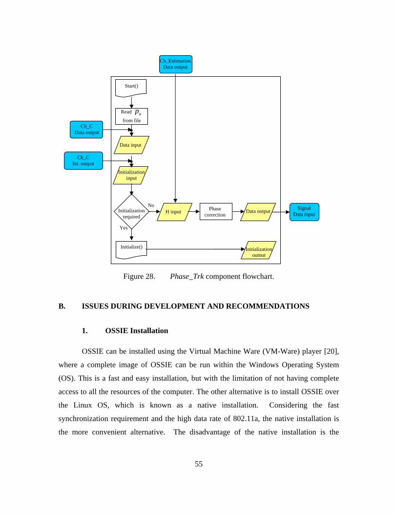
55
Figure 28. Phase_Trk component flowchart.
B. ISSUES DURING DEVELOPMENT AND RECOMMENDATIONS
1. OSSIE Installation
OSSIE can be installed using the Virtual Machine Ware (VM-Ware) player [20],
where a complete image of OSSIE can be run within the Windows Operating System
(OS). This is a fast and easy installation, but with the limitation of not having complete
access to all the resources of the computer. The other alternative is to install OSSIE over
the Linux OS, which is known as a native installation. Considering the fast
synchronization requirement and the high data rate of 802.11a, the native installation is
the more convenient alternative. The disadvantage of the native installation is the
Data input
Initialization input
Initialization required
Initialize()
Yes
No
Ch_C Data output
Start()
Read np
from file .
.
Phase correction
Ch_C Ini. output
Data output Signal Data input
Initialization output
H input
Ch_Estimation Data output
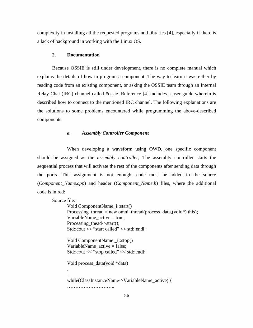
56
complexity in installing all the requested programs and libraries [4], especially if there is
a lack of background in working with the Linux OS.
2. Documentation
Because OSSIE is still under development, there is no complete manual which
explains the details of how to program a component. The way to learn it was either by
reading code from an existing component, or asking the OSSIE team through an Internal
Relay Chat (IRC) channel called #ossie. Reference [4] includes a user guide wherein is
described how to connect to the mentioned IRC channel. The following explanations are
the solutions to some problems encountered while programming the above-described
components.
a. Assembly Controller Component
When developing a waveform using OWD, one specific component
should be assigned as the assembly controller, The assembly controller starts the
sequential process that will activate the rest of the components after sending data through
the ports. This assignment is not enough; code must be added in the source
(Component_Name.cpp) and header (Component_Name.h) files, where the additional
code is in red:
Source file: Void ComponentName_i::start() Processing_thread = new omni_thread(process_data,(void*) this); VariableName_active = true; Processing_thead->start(); Std::cout << “start called” << std::endl; Void ComponentName _i::stop() VariableName_active = false; Std::cout << “stop called” << std::endl; Void process_data(void *data) . . while(ClassInstanceName->VariableName_active) { ………………………..

57
} //while ClassInstanceName ->processing_thread->exit(); Header file: // list components provides and uses ports
Bool VariableName_active;
b. FFTW Library
When compiling a library or software in Linux, four command steps are
required:
• ./reconf
• ./configure
• make
• su –c “make install” (as root)
In the case of fftw, the following options should be included in the
configure command step:
./configure --enable-single --enable-shared --enable-threads --enable-float.
A specific library called lfftw3f must be included, in order to be able to
operate with floating point numbers. If after typing the make command at the prompt, the
compiler complains about an undefined reference to fftwf, the library –lfftw3f should be
included by typing the following at the command prompt:
g++ -Wall –g -02 –I/usr/local/include –pthread –L/usr/local/lib –o ComponentName ComponentName.o –lomniORB4 –lomniDynamic4 –lomnithread –L/usr/local/lib –lossieidl –lossieeparser –lossieecf –lfftw3f –L/usr/local/lib –lstandardInterfaces
Now the library lfftw3f (in red) has been added to the rest of the required
libraries. This process should be performed any time a component using this library is
edited.

58
THIS PAGE INTENTIONALLY LEFT BLANK
59
V. 802.11A WAVEFORM AND TESTING
A. 802.11A SYNCHRONIZATION WAVEFORM
The components developed in this thesis form part of a complete core of
components needed in an 802.11a receiver. As mentioned in I.C.1, the OSSIE
components developed by Leong [7] consider the demodulation and decoding stage of the
receiver assuming an ideal channel. In order to design a complete receiver, a front-end is
required to obtain the baseband digital samples, as well as the equivalent software
component to control the hardware. Therefore, the general structure of the receiver
would be as described in Figure 29.
Figure 29. 802.11a component core structure.
After having available all the required components and hardware, the next step is
to apply the necessary connections through a waveform, which is developed using the
OWD tool from OSSIE. Regarding the synchronization stage, the part of the waveform
that achieves this task will receive the digital samples from the hardware control
component, and output result samples to the decodification stage components. Figure 30
depicts a simple model of the synchronization part of the waveform, where the
components are shown inside the blue block of Figure 29.
Synchronization stage
components
Decodification stage
components
Hardware Control
component
Front-end
Computer
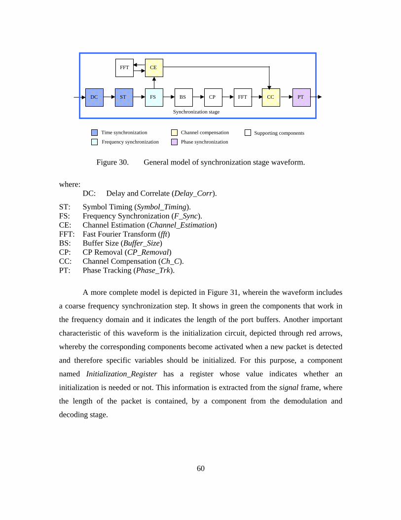
60
Figure 30. General model of synchronization stage waveform.
where: DC: Delay and Correlate (Delay_Corr).
ST: Symbol Timing (Symbol_Timing). FS: Frequency Synchronization (F_Sync). CE: Channel Estimation (Channel_Estimation) FFT: Fast Fourier Transform (fft) BS: Buffer Size (Buffer_Size) CP: CP Removal (CP_Removal) CC: Channel Compensation (Ch_C). PT: Phase Tracking (Phase_Trk).
A more complete model is depicted in Figure 31, wherein the waveform includes
a coarse frequency synchronization step. It shows in green the components that work in
the frequency domain and it indicates the length of the port buffers. Another important
characteristic of this waveform is the initialization circuit, depicted through red arrows,
whereby the corresponding components become activated when a new packet is detected
and therefore specific variables should be initialized. For this purpose, a component
named Initialization_Register has a register whose value indicates whether an
initialization is needed or not. This information is extracted from the signal frame, where
the length of the packet is contained, by a component from the demodulation and
decoding stage.
DC ST FS
CE FFT
BS CP CC FFT PT
Synchronization stage
Time synchronization
Frequency synchronization
Channel compensation
Phase synchronization
Supporting components
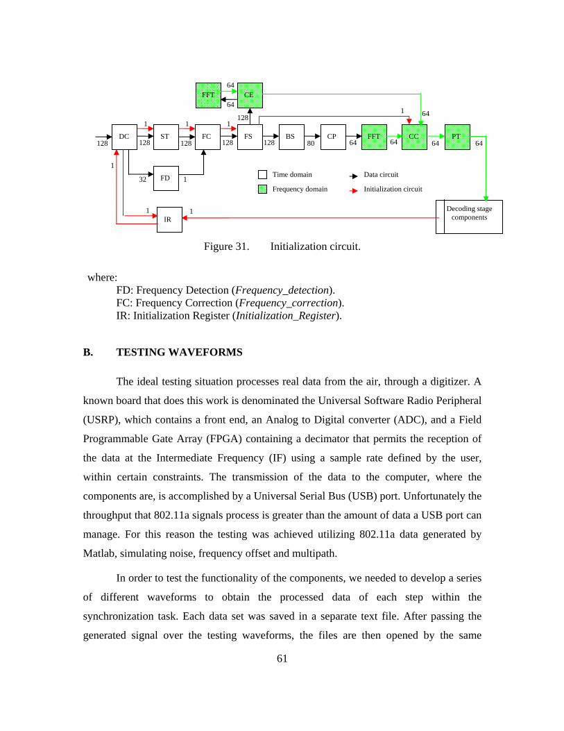
61
Figure 31. Initialization circuit.
where: FD: Frequency Detection (Frequency_detection). FC: Frequency Correction (Frequency_correction). IR: Initialization Register (Initialization_Register).
B. TESTING WAVEFORMS
The ideal testing situation processes real data from the air, through a digitizer. A
known board that does this work is denominated the Universal Software Radio Peripheral
(USRP), which contains a front end, an Analog to Digital converter (ADC), and a Field
Programmable Gate Array (FPGA) containing a decimator that permits the reception of
the data at the Intermediate Frequency (IF) using a sample rate defined by the user,
within certain constraints. The transmission of the data to the computer, where the
components are, is accomplished by a Universal Serial Bus (USB) port. Unfortunately the
throughput that 802.11a signals process is greater than the amount of data a USB port can
manage. For this reason the testing was achieved utilizing 802.11a data generated by
Matlab, simulating noise, frequency offset and multipath.
In order to test the functionality of the components, we needed to develop a series
of different waveforms to obtain the processed data of each step within the
synchronization task. Each data set was saved in a separate text file. After passing the
generated signal over the testing waveforms, the files are then opened by the same
DC ST FS
CE FFT
BS CP CC FFT PT
Decoding stage components
FC
FD
IR
Time domain
Frequency domain Initialization circuit
Data circuit
128 128 128 128
128
128 64 64 64 64
64
64
80
32 1
1
1
1 1 1
1 64
1
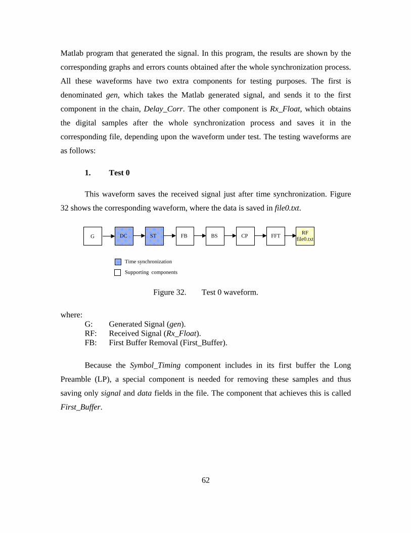
62
Matlab program that generated the signal. In this program, the results are shown by the
corresponding graphs and errors counts obtained after the whole synchronization process.
All these waveforms have two extra components for testing purposes. The first is
denominated gen, which takes the Matlab generated signal, and sends it to the first
component in the chain, Delay_Corr. The other component is Rx_Float, which obtains
the digital samples after the whole synchronization process and saves it in the
corresponding file, depending upon the waveform under test. The testing waveforms are
as follows:
1. Test 0
This waveform saves the received signal just after time synchronization. Figure
32 shows the corresponding waveform, where the data is saved in file0.txt.
Figure 32. Test 0 waveform.
where: G: Generated Signal (gen). RF: Received Signal (Rx_Float). FB: First Buffer Removal (First_Buffer).
Because the Symbol_Timing component includes in its first buffer the Long
Preamble (LP), a special component is needed for removing these samples and thus
saving only signal and data fields in the file. The component that achieves this is called
First_Buffer.
DC ST FB BS CP RF file0.txt FFT
Time synchronization
Supporting components
G
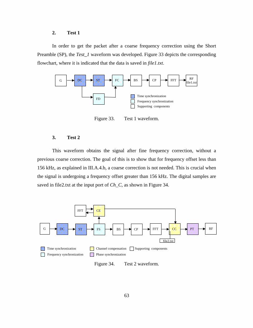
63
2. Test 1
In order to get the packet after a coarse frequency correction using the Short
Preamble (SP), the Test_1 waveform was developed. Figure 33 depicts the corresponding
flowchart, where it is indicated that the data is saved in file1.txt.
Figure 33. Test 1 waveform.
3. Test 2
This waveform obtains the signal after fine frequency correction, without a
previous coarse correction. The goal of this is to show that for frequency offset less than
156 kHz, as explained in III.A.4.b, a coarse correction is not needed. This is crucial when
the signal is undergoing a frequency offset greater than 156 kHz. The digital samples are
saved in file2.txt at the input port of Ch_C, as shown in Figure 34.
Figure 34. Test 2 waveform.
FS
CE FFT
BS CP CC FFT PT
Time synchronization
Frequency synchronization
Channel compensation
Phase synchronization
Supporting components
DC ST RF G
file2.txt
DC ST FC BS CP RF file1.txt
FFT
Time synchronization
Supporting components
G
FD Frequency synchronization
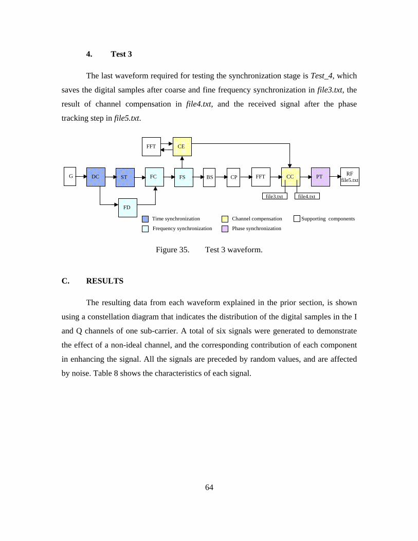
64
4. Test 3
The last waveform required for testing the synchronization stage is Test_4, which
saves the digital samples after coarse and fine frequency synchronization in file3.txt, the
result of channel compensation in file4.txt, and the received signal after the phase
tracking step in file5.txt.
Figure 35. Test 3 waveform.
C. RESULTS
The resulting data from each waveform explained in the prior section, is shown
using a constellation diagram that indicates the distribution of the digital samples in the I
and Q channels of one sub-carrier. A total of six signals were generated to demonstrate
the effect of a non-ideal channel, and the corresponding contribution of each component
in enhancing the signal. All the signals are preceded by random values, and are affected
by noise. Table 8 shows the characteristics of each signal.
FS
CE FFT
BS CP CC FFT PT FC
FD
Time synchronization
Frequency synchronization
Channel compensation
Phase synchronization
Supporting components
DC ST G
file3.txt file4.txt
RF file5.txt
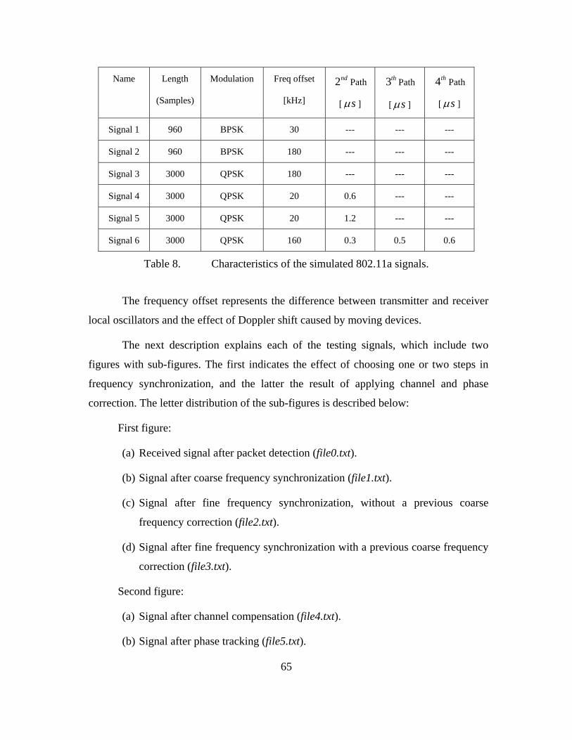
65
Name Length
(Samples)
Modulation Freq offset
[kHz]
2nd Path
[ sµ ]
3th Path
[ sµ ]
4th Path
[ sµ ]
Signal 1 960 BPSK 30 --- --- ---
Signal 2 960 BPSK 180 --- --- ---
Signal 3 3000 QPSK 180 --- --- ---
Signal 4 3000 QPSK 20 0.6 --- ---
Signal 5 3000 QPSK 20 1.2 --- ---
Signal 6 3000 QPSK 160 0.3 0.5 0.6
Table 8. Characteristics of the simulated 802.11a signals.
The frequency offset represents the difference between transmitter and receiver
local oscillators and the effect of Doppler shift caused by moving devices.
The next description explains each of the testing signals, which include two
figures with sub-figures. The first indicates the effect of choosing one or two steps in
frequency synchronization, and the latter the result of applying channel and phase
correction. The letter distribution of the sub-figures is described below:
First figure:
(a) Received signal after packet detection (file0.txt).
(b) Signal after coarse frequency synchronization (file1.txt).
(c) Signal after fine frequency synchronization, without a previous coarse
frequency correction (file2.txt).
(d) Signal after fine frequency synchronization with a previous coarse frequency
correction (file3.txt).
Second figure:
(a) Signal after channel compensation (file4.txt).
(b) Signal after phase tracking (file5.txt).
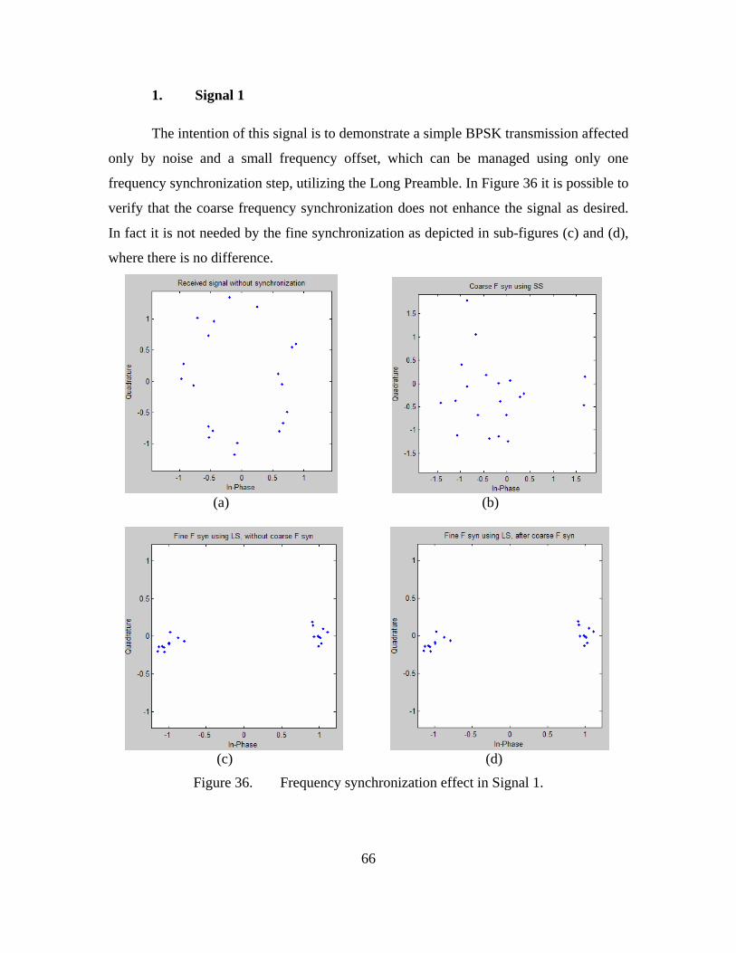
66
1. Signal 1
The intention of this signal is to demonstrate a simple BPSK transmission affected
only by noise and a small frequency offset, which can be managed using only one
frequency synchronization step, utilizing the Long Preamble. In Figure 36 it is possible to
verify that the coarse frequency synchronization does not enhance the signal as desired.
In fact it is not needed by the fine synchronization as depicted in sub-figures (c) and (d),
where there is no difference.
(a) (b)
(c) (d)
Figure 36. Frequency synchronization effect in Signal 1.
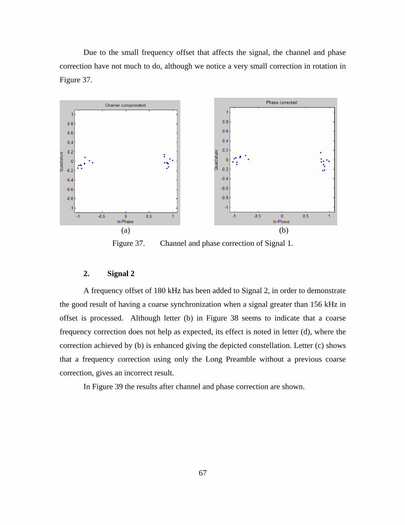
67
Due to the small frequency offset that affects the signal, the channel and phase
correction have not much to do, although we notice a very small correction in rotation in
Figure 37.
(a) (b)
Figure 37. Channel and phase correction of Signal 1.
2. Signal 2
A frequency offset of 180 kHz has been added to Signal 2, in order to demonstrate
the good result of having a coarse synchronization when a signal greater than 156 kHz in
offset is processed. Although letter (b) in Figure 38 seems to indicate that a coarse
frequency correction does not help as expected, its effect is noted in letter (d), where the
correction achieved by (b) is enhanced giving the depicted constellation. Letter (c) shows
that a frequency correction using only the Long Preamble without a previous coarse
correction, gives an incorrect result.
In Figure 39 the results after channel and phase correction are shown.
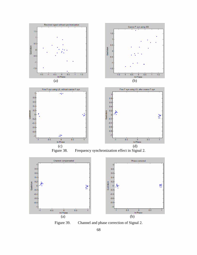
68
(a) (b)
(c) (d)
Figure 38. Frequency synchronization effect in Signal 2.
(a) (b)
Figure 39. Channel and phase correction of Signal 2.
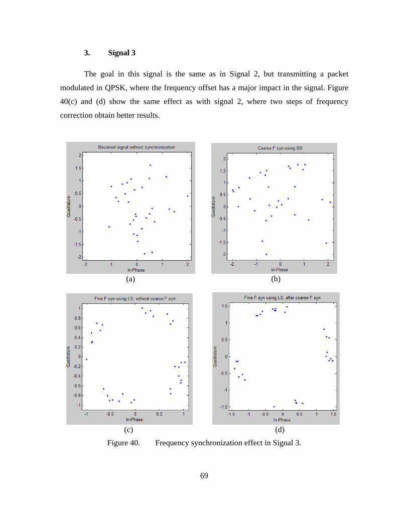
69
3. Signal 3
The goal in this signal is the same as in Signal 2, but transmitting a packet
modulated in QPSK, where the frequency offset has a major impact in the signal. Figure
40(c) and (d) show the same effect as with signal 2, where two steps of frequency
correction obtain better results.
(a) (b)
(c) (d)
Figure 40. Frequency synchronization effect in Signal 3.
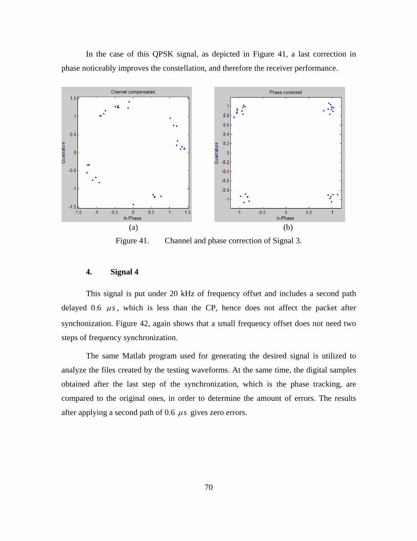
70
In the case of this QPSK signal, as depicted in Figure 41, a last correction in
phase noticeably improves the constellation, and therefore the receiver performance.
(a) (b)
Figure 41. Channel and phase correction of Signal 3.
4. Signal 4
This signal is put under 20 kHz of frequency offset and includes a second path
delayed 0.6 sµ , which is less than the CP, hence does not affect the packet after
synchonization. Figure 42, again shows that a small frequency offset does not need two
steps of frequency synchronization.
The same Matlab program used for generating the desired signal is utilized to
analyze the files created by the testing waveforms. At the same time, the digital samples
obtained after the last step of the synchronization, which is the phase tracking, are
compared to the original ones, in order to determine the amount of errors. The results
after applying a second path of 0.6 sµ gives zero errors.
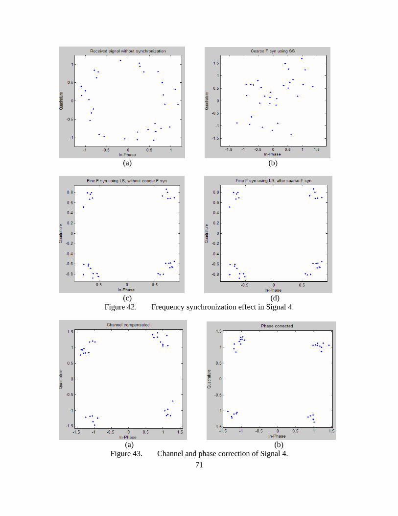
71
(a) (b)
(c) (d)
Figure 42. Frequency synchronization effect in Signal 4.
(a) (b)
Figure 43. Channel and phase correction of Signal 4.
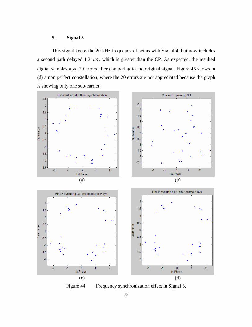
72
5. Signal 5
This signal keeps the 20 kHz frequency offset as with Signal 4, but now includes
a second path delayed 1.2 sµ , which is greater than the CP. As expected, the resulted
digital samples give 20 errors after comparing to the original signal. Figure 45 shows in
(d) a non perfect constellation, where the 20 errors are not appreciated because the graph
is showing only one sub-carrier.
(a) (b)
(c) (d)
Figure 44. Frequency synchronization effect in Signal 5.
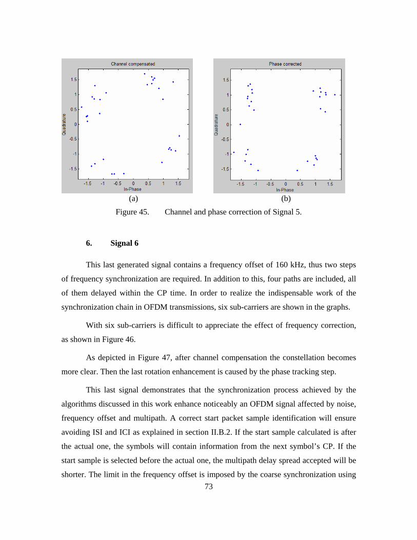
73
(a) (b)
Figure 45. Channel and phase correction of Signal 5.
6. Signal 6
This last generated signal contains a frequency offset of 160 kHz, thus two steps
of frequency synchronization are required. In addition to this, four paths are included, all
of them delayed within the CP time. In order to realize the indispensable work of the
synchronization chain in OFDM transmissions, six sub-carriers are shown in the graphs.
With six sub-carriers is difficult to appreciate the effect of frequency correction,
as shown in Figure 46.
As depicted in Figure 47, after channel compensation the constellation becomes
more clear. Then the last rotation enhancement is caused by the phase tracking step.
This last signal demonstrates that the synchronization process achieved by the
algorithms discussed in this work enhance noticeably an OFDM signal affected by noise,
frequency offset and multipath. A correct start packet sample identification will ensure
avoiding ISI and ICI as explained in section II.B.2. If the start sample calculated is after
the actual one, the symbols will contain information from the next symbol’s CP. If the
start sample is selected before the actual one, the multipath delay spread accepted will be
shorter. The limit in the frequency offset is imposed by the coarse synchronization using
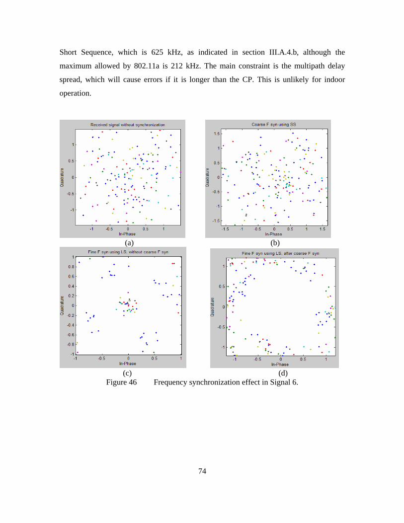
74
Short Sequence, which is 625 kHz, as indicated in section III.A.4.b, although the
maximum allowed by 802.11a is 212 kHz. The main constraint is the multipath delay
spread, which will cause errors if it is longer than the CP. This is unlikely for indoor
operation.
(a) (b)
(c) (d)
Figure 46 Frequency synchronization effect in Signal 6.
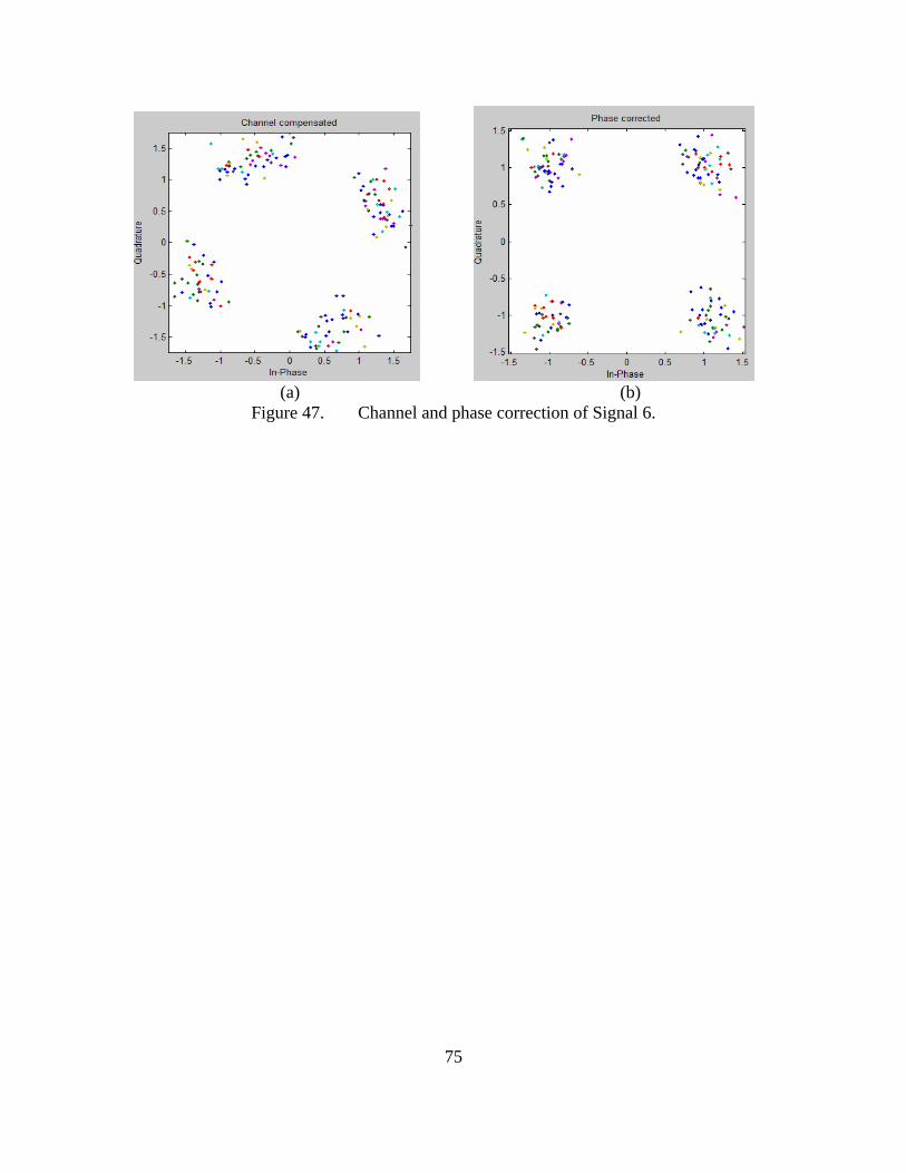
75
(a) (b)
Figure 47. Channel and phase correction of Signal 6.

76
THIS PAGE INTENTIONALLY LEFT BLANK
77
VI. CONCLUSIONS AND FUTURE WORK
A. SUMMARY OF WORK
This thesis describes the design of a synchronization stage for an 802.11a
software defined receiver. The software used to accomplish this goal was OSSIE, which
includes a component and waveform development tool called the OWD. The application
is based on the development of components for each specific synchronization type
required in an OFDM signal transmission. One of the goals was developing these
components using an open architecture to allow reuse for other OFDM standards.
The use of Matlab at the beginning of the work was essential for verifying the
correct implementation of the algorithms obtained from the literature. After this process
the next step was programming the components in OSSIE and testing them against the
results obtained in Matlab.
Due to the throughput that 802.11a signals process and the limitations of our
hardware, the testing part of this work was based on simulated data generated by Matlab,
which used the standard packet structure affected by noise, frequency offset and
multipath. The results obtained showed the correct functionality of the components
through a visual demonstration using constellation diagrams, and a data comparison
against the generated signal, giving the error count after the synchronization stage
performed by OSSIE.
B. SUGGESTED FUTURE WORK
In order to obtain a complete and efficient 802.11a waveform implemented in
OSSIE, the following future work is recommended.
1. Demodulation and Codification Components Upgrade
The group of components developed by Leong [7], should be upgraded to the
current version of OSSIE, which is 0.6.1, and integrated with the synchronization
78
components designed in this work. Additionally, the following modifications should be
performed to fulfill the structure followed by the synchronization components:
a. Initialization Circuit
The decodification component in charge of extracting the information of
signal frame should have a dedicated port to inform the Initialization_Register
component when the current packet has ended. Another way to accomplish this is to pass
the Initialization_Register the length of the packet and make the necessary modifications
to calculate when the packet will end.
b. Connection Between Synchronization and Decoding Components
When creating the 802.11a waveform, the last component of the
synchronization stage that should be considered is Phase_Trk. The first component in the
decodification stage should be the one in charge of the signal frame recovery.
2. Real Data Test
After having all the components working properly, the next step is to test the
802.11a waveform with real data from the air. The aforementioned USRP board is
limited to the data rate accepted by the USB port, which is not enough to manage an
802.11a waveform. A recently announcement from Ettus, the USRP manufacturer,
indicates that a new USRP is under development, which will include an Ethernet port that
will permit a much greater transfer rate. With this new board, the USRP2, it will be
possible to send an 802.11a sampled signal to the PC and process the data in the
corresponding waveform. A USRP control component should be developed in order to
read the digitized signal and send the samples to the first component in the
synchronization stage, which is Delay_Corr.
79
LIST OF REFERENCES
[1] IEEE Std 802.11g-2003, “Part 11: Wireless LAN Medium Access Control (MAC) and Physical Layer (PHY) specifications. Further Higher Data Rates Extension in the 2.4 GHz Band.”
[2] Afshin Niktash, Rafael Maestre and Nader Bagherzadeh, “A Case Study of
Performing OFDM Kernels on a Novel Reconfigurable DSP Architecture,” MILCOM 2005.
[3] JTRS, “Software Communications Architecture Specification,” Version 2.2.2,
May 2006. [4] OSSIE Projects, http://ossie.mprg.org/OSSIE_Projects, last accessed on July
2007. [5] Uprenda Ramdat, “Software Communications Architecture (SCA) Compliant
Software Defined Radio Design for Interim Standard 95B (IS-95B) Transceive,” Master Thesis, Naval Postgraduate School, March 2007.
[6] Low Kian Way, “Software Communications Architecture (SCA) Compliant
Software Defined Radio Design for IEEE 802.16 Wireless MAN-OFDM Transceiver,” Naval Postgraduate School, December 2006.
[7] Leong Wai Kiat Chris, “Software Defined Radio Design for an IEEE 802.11a
Transceiver Using Open Source Software Communications Architecture (SCA) Implementation::Embedded (OSSIE),” Naval Postgraduate School, December 2006.
[8] Vikram Sardana, “Extending the Range of the 802.11g WLAN Through improved
Synchronization Techniques,” Master Thesis, Naval Postgraduate School, June 2007.
[9] Edited by Walter Tuttlebee, “Software Defined Radio,” Wiley 2002. [10] “Definition of Software Communication Architecture, Wikipedia,”
http://en.wikipedia.org/wiki/ Software Communication Architecture, last accessed on June 2007.
[11] Carlos R. Aguayo Gonzalez, “Design and implementation of an Efficient SCA
Framework for Software-Defined Radios,” Master Thesis, Virginia Polytechnic Institute and State University, 2006.
[12] “Definition of OSSIE.” http://ossie.mprg.org, last accessed on June 2007.
80
[13] Richard Van Nee, Ramjee Prasad, “OFDM for Wireless Multimedia
Communication,” 1st sd., Artech House Publishers, 2000. [14] Roberto Cristi, Notes from course EC-4910: “DSP for Wireless Communication,”
2006. [15] Juha Heiskala, John Terry, “OFDM Wireless LANs: A Theoretical Practical
Guide,” SAMS Publishing, 2004. [16] Ramjee Prasad, “OFDM for Wireless Communication Systems,” 1st sd., Artech
House Publishers, 2004. [17] IEEE Std 802.11a-1999 (Revision 2003), “Part 11: Wireless LAN Medium
Access Control (MAC) and Physical Layer (PHY) specifications. High-speed Physical Layer in the 5 GHz Band.”
[18] Jacob A. DePriest. “A Practical Approach to Rapid Prototyping of SCA
Waveforms,” Master Thesis, Virginia Polytechnic Institute and State University, 2006.
[19] Matteo Frigo, Steven G. Johnson. FFTW library from MIT. Website:
www.fftw.org, last accessed on June 2007. [20] VMware Website:”Run Virtual Machines on your PC for Free”
http://www.vmware.com/products/player/, last accessed on September 2007.
81
INITIAL DISTRIBUTION LIST
1. Defense Technical Information Center Ft. Belvoir, VA 2. Dudley Knox Library
Naval Postgraduate School Monterey, CA
3. Professor Jeffrey B. Knorr
Chairman, Code EC Department of Electrical and Computer Engineering Naval Postgraduate School Monterey, CA
4. Assistant Professor Frank Kragh, Code EC/Kh Department of Electrical and Computer Engineering Naval Postgraduate School Monterey, CA 5. Professor Roberto Cristi, Code EC/Cx
Department of Electrical and Computer Engineering Naval Postgraduate School Monterey, CA
6. Ray Cole
Networks and Communication Systems Branch U.S. Naval Research Laboratory Washington, DC
7. Professor Carl Dietrich
Virginia Polytechnic Institute and State University Blacksburg, VA
8. Professor Jeffrey H. Reed
Virginia Polytechnic Institute and State University Blacksburg, VA
9. Ms. Donna Miller Department of Electrical and Computer Engineering Naval Postgraduate School Monterey, CA
82
10. LCDR Vikram Sardana USN, N39 Command Carrier Strike Group 7 Unit 25061
11. LCDR Juan Luis Sanfuentes Chilean Navy Valparaiso Chile