Social Security and the Evolution of Elderly Poverty

Gary V. Engelhardt Department of Economics and

Center for Policy Research 426 Eggers Hall

Syracuse University Syracuse, NY 13210

gvengelh@maxwell.syr.edu

Jonathan Gruber Department of Economics

MIT E52-355

50 Memorial Drive Cambridge, MA 02142

and NBER gruberj@mit.edu

March, 2004

Abstract

We use data from the March 1968-2001 Current Population Surveys to document the evolution of elderly poverty over this time period, and to assess the causal role of the Social Security program in reducing poverty rates. We develop an instrumental variable approach that relies on the large increase in benefits for birth cohorts from 1885 through 1916, and the subsequent decline and flattening of real benefits growth due to the Social Securing “notch”, to estimate the causal effect of Social Security on elderly poverty. Our findings suggest that over all elderly families the elasticity of poverty to benefits is roughly unitary. This suggests that reductions in Social Security benefits would significantly alter the poverty of the elderly.

Prepared for the Berkeley Symposium on Poverty, the Distribution of Income, and Public Policy. We are very grateful to David Card, Ronald Lee, John Quigley, Timothy Smeeding, and Symp osium participants for comments and Cindy Perry for excellent research assistance. The views of the paper are those of the authors and do not reflect the views of the National Bureau of Economic Research, MIT, or Syracuse University.

2

One of the most striking trends in elderly well-being in the twentieth century was the

dramatic decline in income poverty among the elderly. The official poverty rate of those 65

years and older was 35 percent in 1960, more than twice that of the non-elderly (those 18-64),

and had fallen to 10 percent by 1995, below that for the non-elderly. Smolensky, Danziger and

Gottschalk (1988) found similar steep declines in elderly poverty back to 1939. This poverty

reduction exceeded that for any other group in society.

The rapid growth in Social Security benefits in the post-World War II period is often

cited as a major factor in elderly poverty reduction. This conclusion is based on evidence such

as that shown in Figure 1, which plots both the elderly poverty rate and Social Security program

expenditures per capita over time; the figure is rescaled so that both series fit on the same graph.

There is a striking negative association between these series, with elderly poverty declining

rapidly as the Social Security program grows quickly in the 1960s and 1970s, and then declining

more slowly as program growth slows in the 1980s and 1990s. One concern with potential

reforms to the Social Security system is that, to the extent they effectively involve benefit

reduction, the gains in elderly poverty reduction over the last forty years may be reversed.

Our goal in this paper is to assess the role of Social Security in driving this reduction in

elderly poverty. We begin with time series evidence on the growth in Social Security and the

decline in elderly poverty. We consider both absolute and relative measures of elderly poverty,

as well as the heterogeneity in the evolution of elderly poverty. In particular, we consider first

whether these changes in poverty were reflected equally among the oldest old, who start with

much higher poverty rates, and the youngest old; as well as whether the trends were comparable

3

across marital status groups, comparing elders who are married, divorced, widowed, and never

married.

We then assess the causal role of Social Security in explaining these trends. We outline

the econometric problems in the previous literature on the impact of Social Security on elderly

income poverty and propose an instrumental variable procedure to circumvent these difficulties.

We then examine the effect on poverty of the large changes in Social Security benefits for

cohorts born in the late 19th and early 20th centuries. Of particular interest is the sharp benefits

changes for birth cohorts from 1906 through 1926. The early cohorts in this range saw enormous

exogenous increases in Social Security benefits, partly due to double indexation of the system in

the early 1970s. This doub le indexing was ended in the 1977 Amendments to the Social Security

Act that generated the so-called “benefits notch.” The 1977 law grandfathered all individuals

born before January 1, 1917, under the old benefit rules, but those born in 1917-1921 received

benefit reductions that were as much as 20 percent lower than observationally equivalent

individuals in the 1916 birth cohort. After 1921, benefits were roughly constant in real terms. It

is this variation that was first identified by Krueger and Pischke (1992) as a fruitful means of

identifying the behavioral effects of Social Security, in their case in the context of retirement

decisions. We follow their methodology to define an instrumental variable for observed Social

Security benefits.1

We carry out this analysis using data from 1967 through 2000 from the March Current

Population Survey (CPS), to study those elderly born in 1885 through 1930. We use these data

to form income measures for elderly households and families. Elderly households are all living

1 In related papers, Snyder and Evans (2002) and Engelhardt, Gruber, and Perry (2002) used the notch to examine the effect of income on mortality and living arrangements, respectively.

4

units in which an elderly person resides; elderly families consist of an elder and his/her spouse.

So if an elderly couple co-resides with their children, they are in the same household, but

different families.

We have several findings of interest. First, while there has been a major decline in

absolute poverty among elderly households, that decline has been much smaller for relative

poverty, which did not decrease in the 1980s and 1990s. This raises the important question of

whether the elderly should or should not share in the increases in the standard of living realized

by the non-elderly. Income inequality has also exploded among the elderly in the 1990s.

Second, these changes in the income position of low income elders are fairly similar

across age groups, with all age groups following the same basic patterns outlined above. Third,

there are important differences in these patterns by marital status group. In particular, the

declines in absolute poverty that we see in the data are much stronger for married than for

unmarried elders.

Fourth, we document a major causal role of Social Security in driving these time series

patterns. Increases in Social Security generosity over time are strongly negatively associated

with changes in poverty. There is, however, a weak association with income inequality,

suggesting that Social Security is benefiting higher income elders at the same or higher rate that

it benefits low income elders over this period.

Finally, we illustrate the critical role of elderly living arrangements in driving these

conclusions. As we document, there were stark changes in the living arrangements of the elderly

over the time period we study, with a large shift in living with others to living independently.

Our regression results show that the effect of Social Security on poverty is much stronger for

5

families than for households, in particular for widows/widowers and divorcees. This is

consistent with the findings of Engelhardt, Gruber and Perry (2002) that higher Social Security

benefits cause more independent living among widowed and divorced elders. When those elders

move out on their own, they are in the same family, but they become relatively poor households,

raising the poverty rate among households. This offsets to some extent the measured poverty

reduction among the elderly from higher benefits.

The paper is organized as follows. The next section describes the CPS data. Section III

charts the time-series evolution of elderly income and poverty from 1967-2000. Section IV

outlines the primary method used to determine the impact of Social Security in the previous

literature and describes the construction of the instrumental variable. Section V discusses the

empirical results. There is a brief conclusion.

II. Data Construction

This study uses data from the Current Population Surveys (CPS) of March, 1968 through

2001. Each file is a cross sectional nationally representative sample of households. We restrict

our analysis to cohorts born starting in 1880 (because our sample is very small before that

cohort), and ending in 1935, the youngest cohort that turns 65 in our data.

To construct our main sample, we first assign families within the CPS. For our purposes,

a “family” is defined as the household head, his or her spouse, and any children of the household

head that are living in the household and are under the age of 18. This differs from the CPS

family definition in that we assume any other member of the household is his/her own family,

whereas all individuals related by birth, marriage, and adoption are considered members of the

CPS family. Note that there may be more than one “family” in a given CPS “household” (e.g. if

6

there are multiple non-married elderly living together). Our family definition requires

consistency in relational measures in the CPS household in the annual surveys. Because of

changes in these measures, we were not able to construct our measure of the family prior to the

March, 1968 CPS. We use both families and households as our observational unit.

In order to measure outcomes for any age range, for either households or families, we

weight the full sample of households/families by the number of persons sharing that

household/family in the relevant age range. That is, our estimated poverty rate for 65-69 year

old “households” is the poverty rate over all households containing a 65-69 year old, weighted

by the number of persons age 65-69 in that household. So these are essentially person-weighted

poverty rates.

The questions in the March CPS are about income earned in the previous calendar year,

so that even though we use data from the 1968-2001 surveys, the income data refer to 1967-

2000. Over time, the CPS has provided more disaggregated questions on income sources, and,

for some types of income, has changed the wording of questions. For each year, we used the

most disaggregated income measures to make our poverty measures, which, following official

poverty rates, are based on gross income.2 All income measures were deflated into real 2001

dollars using the all- items Consumer Price Index (CPI).

We begin our analysis with the classic absolute poverty measure, whether a family is

below the federal poverty line. Specifically, for the household- level analysis, we assigned to

each household the poverty threshold for the appropriate household size. Similarly, for the

family- level analysis, we assigned to each family the threshold for the appropriate size, treating

2 In addition, we constructed poverty measures using a set of more aggregated income measures consistently measured across surveys, and the results of our statistical analysis below did not change. We made no attempt to quantify in-kind transfers received (Smeeding, 1986) into our gross income measures.

7

the family as the “household” in the federal threshold definition. We did not incorporate the age

65 and older adjustments for one- and two-person households built into the federal thresholds, so

that we could compare elderly and non-elderly on an equal basis. This absolute measure of

poverty has a number of limitations, however. First, it holds standards of living constant, and

does not allow for productivity growth. Specifically, in a mechanical sense, if there is any real

productivity growth over time, so that real wage growth is positive, then poverty based on the

federal threshold likely will fall over time, because this measure only adjusts for inflation, not

real earnings growth. Second, it is a knife-edge measure that does not capture the depth of

absolute deprivation.

As an alternative, we define a relative measure of the poverty line: 40 percent of the

median income per OECD equivalent of the non-elderly in each calendar year. Non-elderly are

defined as individuals 25-54 years old. We adjust both elderly and non-elderly income by the

OECD equivalence scale. The relative measure has an important feature. It does not hold living

standards constant. Holding real elderly income per equivalent constant, elderly poverty will rise

as median non-elderly income rises. This relative measure will yield poverty rates that are more

likely to be pro-cyclical, as median income rises and falls over the business cycle.

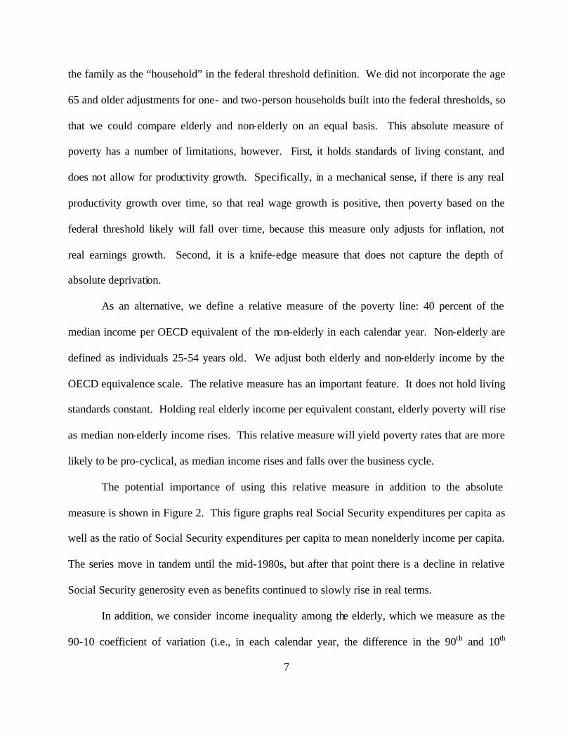
The potential importance of using this relative measure in addition to the absolute

measure is shown in Figure 2. This figure graphs real Social Security expenditures per capita as

well as the ratio of Social Security expenditures per capita to mean nonelderly income per capita.

The series move in tandem until the mid-1980s, but after that point there is a decline in relative

Social Security generosity even as benefits continued to slowly rise in real terms.

In addition, we consider income inequality among the elderly, which we measure as the

90-10 coefficient of variation (i.e., in each calendar year, the difference in the 90th and 10th

8

elderly OECD equivalent income percentiles normalized by mean elderly income). We also

considered other variants of poverty measures. Specifically, we created alternative measures of

the absolute poverty line based on 133, 150, and 200 percent, respectively, of the relative poverty

line based on 25 and 50 percent of the non-elderly median income, respectively, and measures

based on gross and net income. The results did not differ from those presented below. For the

remainder of the analysis, all income measures were based on gross income to be comparable

with the federal poverty thresholds.

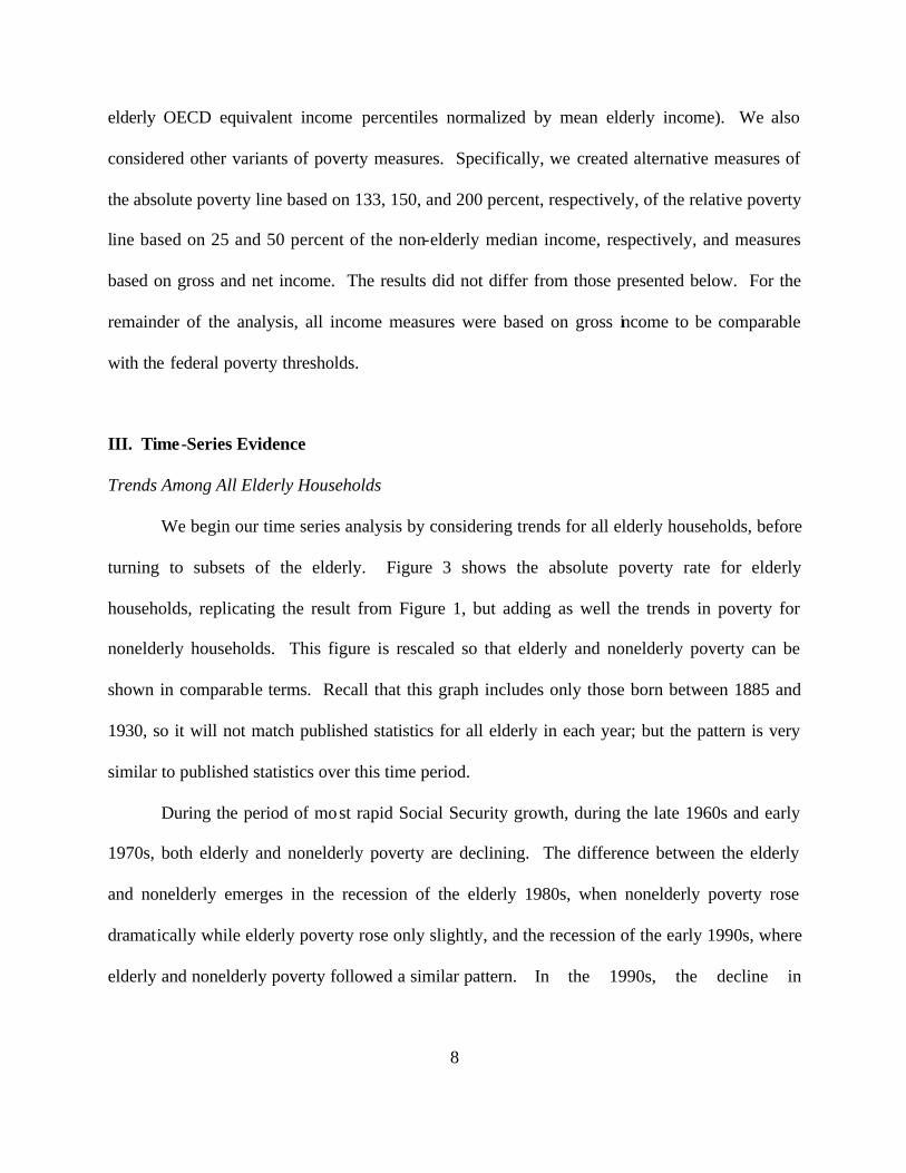
III. Time-Series Evidence

Trends Among All Elderly Households

We begin our time series analysis by considering trends for all elderly households, before

turning to subsets of the elderly. Figure 3 shows the absolute poverty rate for elderly

households, replicating the result from Figure 1, but adding as well the trends in poverty for

nonelderly households. This figure is rescaled so that elderly and nonelderly poverty can be

shown in comparable terms. Recall that this graph includes only those born between 1885 and

1930, so it will not match published statistics for all elderly in each year; but the pattern is very

similar to published statistics over this time period.

During the period of most rapid Social Security growth, during the late 1960s and early

1970s, both elderly and nonelderly poverty are declining. The difference between the elderly

and nonelderly emerges in the recession of the elderly 1980s, when nonelderly poverty rose

dramatically while elderly poverty rose only slightly, and the recession of the early 1990s, where

elderly and nonelderly poverty followed a similar pattern. In the 1990s, the decline in

9

nonelderly poverty was much steeper than the decline in elderly poverty. These findings on the

relative cyclicality of poverty highlight the protective role of Social Security for the elderly.

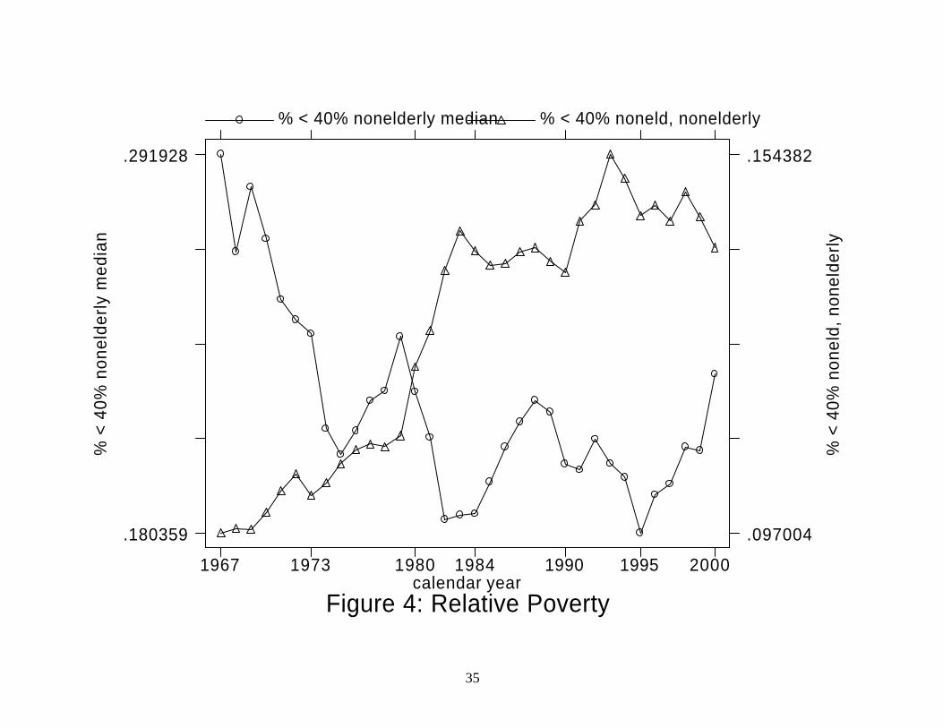
Figure 4 shows the relative poverty rate for the elderly and nonelderly. During the late

1960s and early 1970s, the relative poverty rate of the elderly was falling, just as was the case

with absolute poverty, although in this case the declines came against a backdrop of rising non-

elderly relative poverty. During the 1980s and 1990s, the decline stagnated, so that there was on

net little change in relative poverty from 1980 through 2000. The fact that relative poverty did

not fall, while absolute poverty did, is consistent with the pattern of benefits during the 1980s

and 1990s shown in Figure 2.

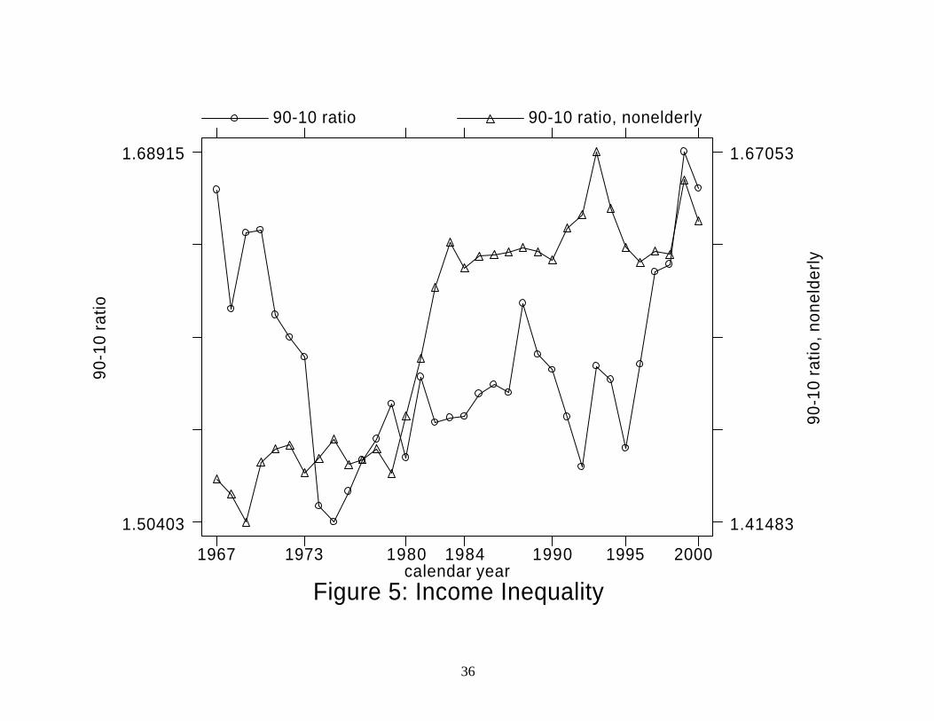
Figure 5 shows the evolution of inequality within the elderly over time. Relative to the

nonelderly, inequality among the elderly declined significantly from the late 1960s through the

early 1990s. But inequality exploded in the late 1990s among the elderly, rising at an even faster

rate than inequality among the non-elderly.

Families vs. Households

The analysis thus far has focused on elderly households, which includes both elders and

others that share their residence. An alternative means of measuring poverty is just to focus on

the elders themselves (and their own spouses and children under 18) in a family- level analysis.

These analyses can potentially yield very different measures of poverty because changes in

Social Security benefits can change the living arrangements of the elderly. A number of studies,

most recent Engelhardt, Gruber and Perry (2002) find that unmarried elders are more likely to

live on their own as their Social Security benefits rise. Engelhardt, Gruber, and Perry (2002)

found that widows were quite sensitive to benefits in their living arrangements, with each 1%

10

rise in benefits found to lead to a 1.3% reduction in the share of widows living with others. In

addition, elderly divorcees were even more income elastic in their living arrangements. But

those who are never married are less elastic, and those are married are not at all elastic. Overall,

averaging across all of these groups, there is a sizeable elasticity of –0.4.

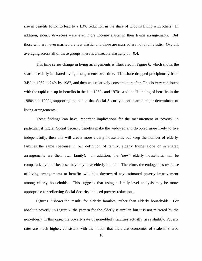
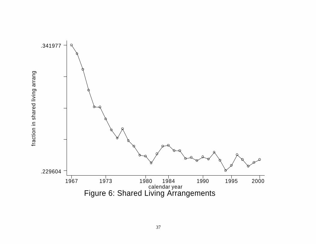
This time series change in living arrangements is illustrated in Figure 6, which shows the

share of elderly in shared living arrangements over time. This share dropped precipitously from

34% in 1967 to 24% by 1982, and then was relatively constant thereafter. This is very consistent

with the rapid run-up in benefits in the late 1960s and 1970s, and the flattening of benefits in the

1980s and 1990s, supporting the notion that Social Security benefits are a major determinant of

living arrangements.

These findings can have important implications for the measurement of poverty. In

particular, if higher Social Security benefits make the widowed and divorced more likely to live

independently, then this will create more elderly households but keep the number of elderly

families the same (because in our definition of family, elderly living alone or in shared

arrangements are their own family). In addition, the “new” elderly households will be

comparatively poor because they only have elderly in them. Therefore, the endogenous response

of living arrangements to benefits will bias downward any estimated poverty improvement

among elderly households. This suggests that using a family- level analysis may be more

appropriate for reflecting Social Security- induced poverty reductions.

Figures 7 shows the results for elderly families, rather than elderly households. For

absolute poverty, in Figure 7, the pattern for the elderly is similar, but it is not mirrored by the

non-elderly in this case; the poverty rate of non-elderly families actually rises slightly. Poverty

rates are much higher, consistent with the notion that there are economies of scale in shared

11

living conditions). Nevertheless, in these time series data, there is no evidence of a major effect

of using families rather than households for the analysis.

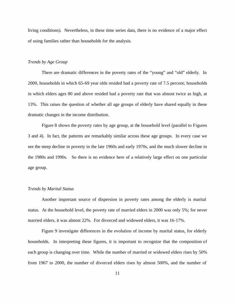
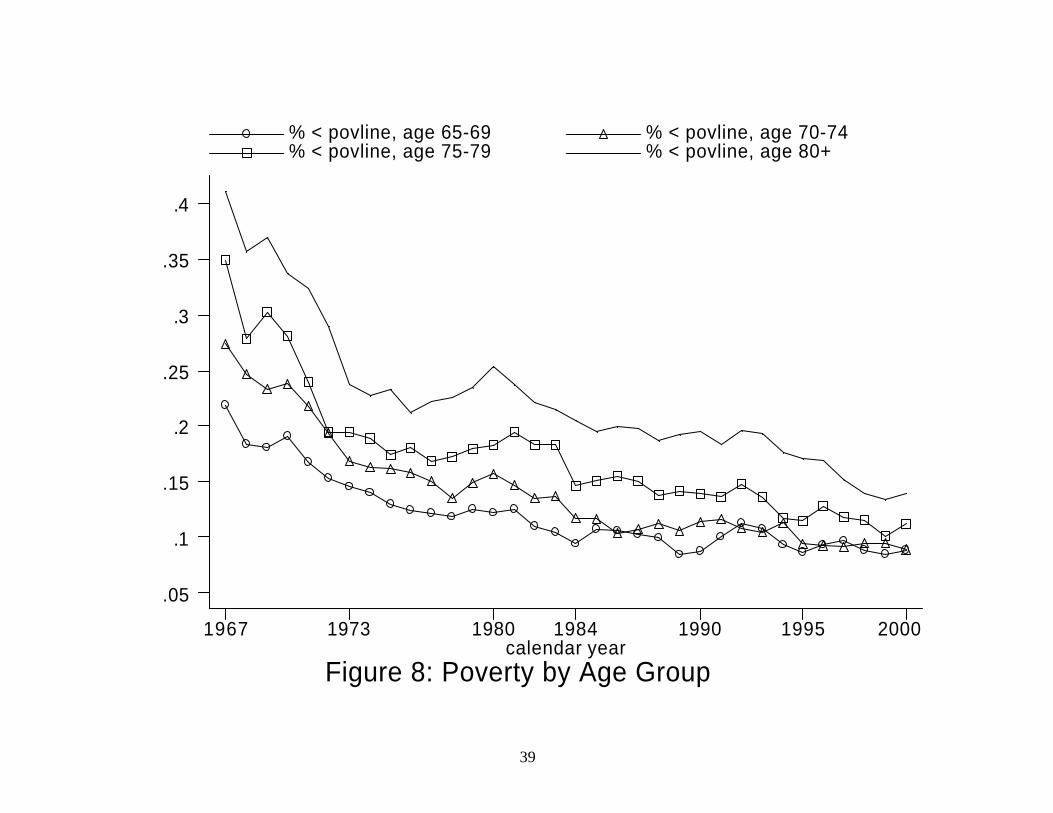
Trends by Age Group

There are dramatic differences in the poverty rates of the “young” and “old” elderly. In

2000, households in which 65-69 year olds resided had a poverty rate of 7.5 percent; households

in which elders ages 80 and above resided had a poverty rate that was almost twice as high, at

13%. This raises the question of whether all age groups of elderly have shared equally in these

dramatic changes in the income distribution.

Figure 8 shows the poverty rates by age group, at the household level (parallel to Figures

3 and 4). In fact, the patterns are remarkably similar across these age groups. In every case we

see the steep decline in poverty in the late 1960s and early 1970s, and the much slower decline in

the 1980s and 1990s. So there is no evidence here of a relatively large effect on one particular

age group.

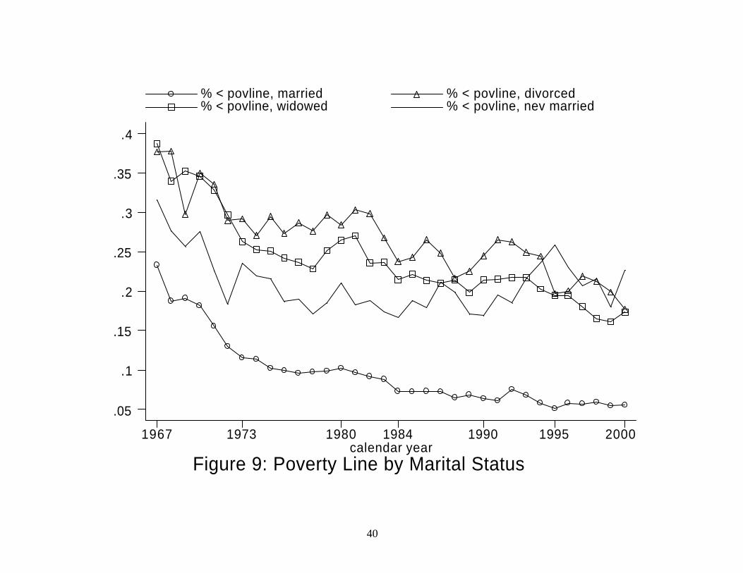
Trends by Marital Status

Another important source of dispersion in poverty rates among the elderly is marital

status. At the household level, the poverty rate of married elders in 2000 was only 5%; for never

married elders, it was almost 22%. For divorced and widowed elders, it was 16-17%.

Figure 9 investigate differences in the evolution of income by marital status, for elderly

households. In interpreting these figures, it is important to recognize that the composition of

each group is changing over time. While the number of married or widowed elders rises by 50%

from 1967 to 2000, the number of divorced elders rises by almost 500%, and the number of

12

never married elders rises by over 300%. Thus, patterns in poverty over time could reflect group

composition changes.

Given this caveat, the results for changes in poverty by marital status are quite

interesting. It appears that the changes over time for all elderly are driven by the married elderly.

The patterns are much stronger for married elderly than for other groups. Particularly striking is

the lack of poverty decline for never married elderly, who start out with the second highest

poverty rate in 1967 and have the highest rate of these groups by 2000.

IV. Identifying the Impact of Social Security

The previous literature on poverty is voluminous, and we do not attempt to review it

here.3 Instead, we focus on the primary method used to measure the impact of public policies on

poverty and how that relates to our instrumental variable identification strategy. Following Jantti

and Danziger (2000), let i and t index elderly sub-group and calendar year, respectively, F be

a function of resources, then ]);([ zyFPit is a poverty measure for some income y and poverty

line z . In addition, let b denote Social Security income, so that

byy +′= , (1)

where y′ is market capital and labor income. In principle, the impact of Social Security on

poverty is

]);([]);(~

[~

zyFPzyFP itit −′=∆ , (2)

where F~ is the counterfactual distribution of market labor and capital income in the absence of

Social Security. In practice, the primary method for analyzing the impact of Social Security on

3 See Jantti and Danziger (2001), Cowell (2001), and Gottschalk and Smeeding (2001) for comprehensive recent reviews of various aspects of this literature.

13

poverty has been to calculate the actual difference in poverty using market income and income

net of taxes and transfers,

]);([]);([ zyFPzyFP itit −′=∆ . (3)

There are three problems with ∆ as a measure of the impact of Social Security on

poverty. First, it misses is any “crowd out” of real behavior. In particular, observed capital and

labor income, y′ , itself may be a function of benefits, b , if, for example, when faced with an

unanticipated and permanent increase in benefits, the elderly leave the labor force earlier, reduce

post-retirement hours of labor supplied, increase consumption and reduce saving, or substitute

independent for shared living arrangements.4 Second, survey-based measures of income might

be subject to reporting error. Third, to the extent that most of the variation in Social Security

benefits that identifies ∆ is time-series in nature, there may omitted variables that are correlated

with changes in poverty rates and Social Security. For example, lifetime earnings, which enter

into Social Security benefit calculations, are affected by aggregate productivity and human

capital accumulation that have been changing across time. However, because the federal poverty

thresholds are inflation-adjusted, but not average earnings adjusted, in a mechanical sense,

poverty rates for successive birth cohorts should be predicted to fall as productivity, human

capital accumulation, and real lifetime earnings have risen. Thus, what might appear as an

inverse correlation between elderly poverty based on absolute measures and Social Security, as

in our figures, may simply be due to rising aggregate productivity. That is, even in the absence

of Social Security having had a causal impact, elderly poverty would appear to have fallen as

4 See Feldstein and Liebman (2001) for a comprehensive recent review of studies on labor supply and saving behavior, Sawhill (1988), Hurd (1990), and Danziger, Haveman, and Plotnick (1981) for earlier reviews. Engelhardt, Gruber, and Perry (2002) review the literature on elderly living arrangements.

14

benefits rose. This would bias estimates toward finding that Social Security lowered elderly

poverty.

Construction of the Instrument

To circumvent these problems we place (3) in a regression framework and construct an

instrumental variable for Social Security benefits independent of omitted time-varying factors

and based on an exogenous measure of lifetime labor income. The variation in this instrument

derives solely from legislative changes in benefits.

To construct our instrument, we note that all of the identifying variation from the Social

Security notch is based on year of birth, and divide the underyling CPS micro data into age-by-

calendar year cells, which, of course, are also year-of-birth cells. The year of birth refers to the

“Social Security beneficiary,” defined as the male person in the family 65 and older. If there is

no male 65 and older, the beneficiary is the oldest never-married female in the family. These

two groups consist of people most likely to have had Social Security benefits based on their own

earnings history, rather than that of their spouse. If there is neither a male nor a never-married

female 65 and older, we assign the Social Security beneficiary to be the divorced or widowed

female that is 65 and older. We assume that her Social Security benefits are based on the

earnings of her former or deceased spouse, assumed to be three years older than her, so that the

“age” of beneficiary is the woman’s age plus three for the purposes of calculating our

instrument.5

5 Three years was the median difference in age between male and female spouses in the 1981 New Beneficiary Survey. An additional factor that influences actual Social Security benefit levels for widows is the age at which the spouse dies (for widows). A widow whose husband dies at a relatively young age will receive less than a widow whose spouse dies at an older age, due to a longer earnings history for the deceased spouse. For a divorcee, the age at which the marriage ends and the duration of the marriage (for divorcees) are also important factors, as divorcees

15

The instrument is based on the notion that Social Security benefits should be constructed

to be identical for each year of birth except for changes in the benefits law. To do so, we first

assigned an earnings history to the 1916 birth cohort. The Annual Statistical Supplement

produced by the Social Security Administration each year contains the median Social Security

earnings by gender for five-year age groups on a yearly basis for the current year as well as years

past. We use median male earnings from these tables. We assigned median earnings at age 22

(from the median earnings for ages 20-24 in 1938), age 27 (from median earnings for ages 25-29

in 1943), etc., in five-year intervals. We then assume a linear trend in earnings in between these

five-year intervals. This method is used through age 60, and earnings are assumed to grow with

inflation for ages beyond 60. We do not use median earnings for workers over 60 because many

of these workers have entered “bridge” jobs, so that the median worker’s earnings at these ages

may not be representative of workers who have remained in their lifetime jobs through age 65.

This generates an earnings history for a median male earner in the cohort born in 1916. We use

the same earnings profile even when assigning benefits to never married females, because we

assume that their earnings profile would more closely resemble that of a male worker than that of

the median female worker.6

Importantly, we want our instrument to vary only with changes in Social Security benefit

rules and do not want to capture changes in earnings profiles due to human capital and

productivity changes in cohorts over time. Therefore, we use the earnings history that we

constructed for the 1916 cohort for all birth cohorts, and simply use the CPI to adjust this

may only claim on their former spouses’ earnings histories if the marriage lasted at least 10 years. Because the March survey did not ask the duration of previous marriages for divorcees or the age at death of the spouse for widows, we could not incorporate these factors into the construction of our instrument. 6 In separate tabulations in the CPS, the median earnings of never ma rried females are significantly more highly correlated with male earnings than with the earnings of all females.

16

earnings profile for inflation for earlier and later cohorts. Thus, all birth cohorts have the same

real earnings trajectory over time. By holding lifetime earnings constant by construction, this

insures that all of the variation in the instrument comes from variation in the benefit formula due

to the law change. We also assume that this prototypical earnings history ends at age 65, so that

we do not incorporate any variation across cohorts in average retirement ages. So we assume all

workers retire at age 65; our results are very similar using an instrument that uses a fixed

distribution of retirement ages from the 1916 cohort.

Our next step is to input the constructed earnings histories into the Social Security

Administration’s ANYPIA program. This program calculates the monthly benefit at retirement

given a date of bir th, date of retirement, and earnings history. ANYPIA gives the monthly

benefit at the date of retirement, which is the primary insurance amount (PIA). We assign

birthdays of June 2 in the particular year of birth and assume that people retire and claim benefits

in June of their retirement year to yield a PIAfor that year of birth..7 Married couples are

assigned 150% of this PIA.

The Social Security Administration periodically increases nominal benefits to adjust for

inflation. To obtain a value for the predicted benefit for a given age and year-of-birth cohort, we

need to account for all “cost of living adjustments” (COLA) until the date of interview. We

calculate the median month in which a given age and year-of-birth cell was interviewed, and

administer all COLA adjustments from the time that the person would have retired through this

date. This produces a predicted (COLA-adjusted) Social Security monthly benefit for each age

and year-of-birth cell. We then multiply by 12 to get the predicted annual benefit.

7 We assume that they claim in June because some cost-of-living (COLA) adjustments were administered in June of a given year, rather than December of a given year. We assume that the beneficiary claims in June so that he will receive any COLA in that year. This prevents variation across years of birth based simply on the timing of the COLA.

17

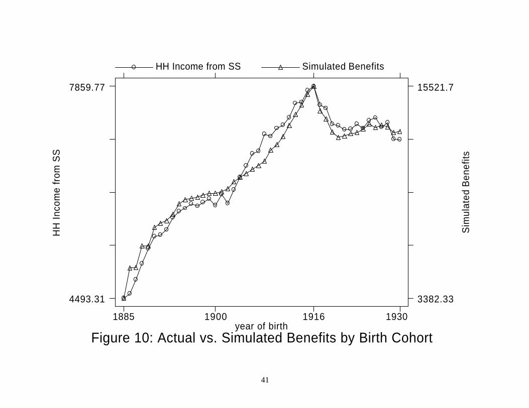
Figure 10 shows the plot of cell mean annual household Social Security income versus

the instrument by year of birth. The variation in benefits, even conditional on constant earnings

histories, is readily apparent in the graph of the instrument. Benefits are rising steadily until

1910, and then ramp up quickly from 1910 through 1916, before falling precipitously in the

1917-1921 period, and then rising more slowly thereafter. The graph of actual Social Security

incomes by cohort tracks this pattern well, with the benefits notch apparent in the data. So there

is a good first stage relationship here: our legislative variation instrument clearly predicts actual

Social Security incomes.

Regression Specification

To examine the effect of Social Security on elderly poverty, we estimate the following

basic specification,

itititit uSSIncomeP ++′= θδ X (4)

where i and t index single year of age and calendar year, respectively. P is poverty (or one of

the other outcome measures used here), SSIncome is the cell mean reported annual Social

Security income, and u is a disturbance term. The parameter θ indicates the change in the

proportion of elderly in poverty for a change in Social Security income. X is a vector of all

other explanatory variables. We specify Xδ ′ as

∑∑==

++′=′1999

1967

90

65 t

Year titt

i

Age iitiitit DDx αγβδ X , (5)

where x is a vector of demographic variables that includes controls for cell means of educational

attainment of the head (high school diploma, some college, and college or advanced degree),

marital status (married, widowed, and divorced in the pooled sample) white, and female. By

18

controlling for these cell characteristics, we control for any other trends in cohort characteristics

that might be correlated with both the legislative changes in benefits determination and with

poverty. Following Krueger and Pischke (1992), we also include in (5) a full set of dummies for

the age of the head, i AgeD , and calendar year dummies, t YearD .8 The age dummies control for

differences across age groups in the outcome measure; the year dummies control for any general

time trends in the outcome measure.

Thus, after controlling for age and calendar year, the variation in SSIncome is based only

upon year of birth. When we then instrument with the variable described above, which we

denote as Z , our model is identified solely by legislative variation in benefits generosity across

birth cohorts, and not any differences in their earnings history. The regression analysis is based

on 950 elderly age-by-year cells. The means of the dependent variable and primary explanatory

variable are shown in Table 1 for each sample.9

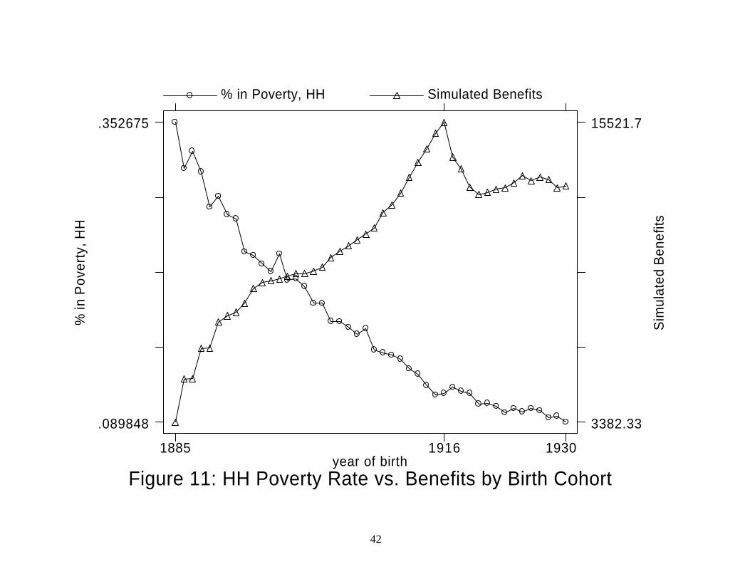
Visual Inspection

To illustrate the nature of the regression results that follow, we begin with a visual

inspection of the data. Figure 11 shows the average poverty rate at ages 65 and older for each

birth cohort, graphed against our instrument for that birth cohort. There is a rapid decline in

poverty for early cohorts, where benefits are rising, and this rate of decline slows substantially

after the notch in 1916, although the decline does continue. This is suggestive of a role for

benefits, but the correspondence is not particularly striking.

8 The excluded group consists of families with heads’ age over 90, observed in calendar year 2000. 9 Descriptive statistics for all variables and samples are available in an appendix from the authors.

19

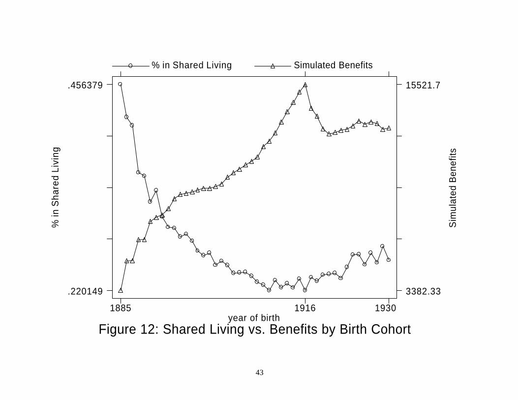
Figure 12 shows a parallel graph for shared living arrangements. Once again, there is a

steep decline in the early years of the sample, when benefits are rising most rapidly, then a

turnaround and rise in shared living arrangements when Social Security benefits fall and flatten.

This evidence is very consistent with a benefits effect on shared living arrangements.

V. Estimation Results

Basic Results

Table 2 shows the grouped OLS and IV estimation results for the full sample that

includes all elderly, where the weights were based on the cell sizes. Standard errors are shown

in parentheses. Each row shows the estimate of θ for the associated outcome measure.

Columns 1 and 2 give the grouped OLS and IV estimates of θ with no other controls,

respectively. Column 3 gives the IV estimates with other controls. In columns 1-3, in which, the

outcome and Social Security measures are in levels, all coefficients are multiplied by 1000 for

ease of interpretation; so, the coefficient shows the impact of a real $1000 rise in annual Social

Security benefits on the outcome. In column 4, the outcome and the Social Security measures

are in logs, so that the coefficients are interpreted as elasticities, and column 5 shows the results

in logs with the X controls. Panel A gives estimates for elderly households and Panel B for

families.

Using the fraction of elderly households below federal poverty threshold (the head-count

ratio) as the dependent variable (row 1, Panel A), a $1000 increase in annual benefits reduces the

poverty rate by 2.8 percentage points (column 1). The IV estimates in columns 2 and 3 imply

decreases in the poverty rate of 3.5 and 3.1 percentage points without and with controls,

respectively. The IV estimates from the log specification with controls in column 5 imply an

20

elasticity of the poverty rate to Social Security benefits of -0.72, so that if benefits were cut by 10

percent, the poverty rate would be expected to rise by 7.2 percent (not percentage points).

Over the 1967-2000 period, the poverty rate for this sample fell from 28.3 percent to 11.6

percent, or by 16.7 percentage points, while the simulated Social Security benefit, Z , rose by

$5760, or 91%. Hence, the IV linear estimate in column 3 implies that the increase in Social

Security benefits of $5760 would lead to a 17.8% decline in poverty rates. The IV log estimate

in column 5 implies that the 91% rise in benefits should have led to a 66% decline in poverty

rates. Both of these estimates are almost exactly the same as the poverty decline experienced by

these elderly, suggesting that Social Security can explain all of the decline.

The first row of panel B shows the estimates of θ for the family- level dataset. The

results for elderly families are much stronger. In column 5, the estimated elasticity of the

poverty rate to Social Security benefits is -1.38, which suggests that a cut in benefits of 10

percent would increase the proportion of elderly families in poverty by 13.8 percent. The IV

linear estimate in column 3 implies that each $1000 increase in Social Security benefit would

cause a 5.7 percent decline in elderly poverty.

At the family level, the poverty rate fell from 39.4 to 16.9%, a decline of 22.5 percentage

points (57% of base value). Applied to the $5760 (91%) rise in benefits over this period, both of

these estimates suggest that, at the family level, poverty actually fell less than it should have

given the rise in benefits. The log estimate suggests that family level poverty should have fallen

by 126% (twice the actual fall), and the level estimate suggests that family level poverty should

have fallen by 33% (50% larger than the actual fall).

The second row of Table 2 gives the estimates of θ for the relative poverty rate.

Increases in Social Security benefits appear to play a strong causal role in reducing poverty for

21

both the levels and log specifications. Once again, there is a much stronger effect for elderly

families than households, a consistent finding throughout the empirical analysis, and one to

which we return below.

The third row of each panel shows the estimated impact of Social Security on our

measure of inequality (the 90-10 difference divided by mean income). For elderly households,

there is a significant reduction in inequality, but for elderly families, this finding is very sensitive

to the inclusion of controls in the model. Overall, the results in Table 2 indicate that Social

Security has played a very significant role in reducing elderly poverty, measured as (absolute and

relative) rates and gaps. However, it may be a fairly blunt instrument at the family level, where

there are only insignificant declines in inequality.

The final row of the table shows the impact of Social Security benefits on shared living

arrangements. There is a sizeable negative effect, with the log estimate suggesting an elasticity

of shared living arrangements of 1.8 with respect to the benefit level. This is an enormous effect,

much larger than is found in Engelhardt, Gruber and Perry (2003) for their full sample.

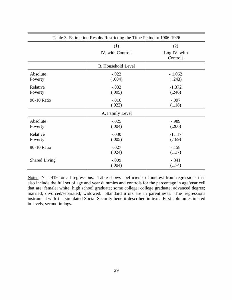
Restricting the Time Period

One disadvantage of the estimation strategy thus far is that it does not focus explicitly on

the “notch” variation in benefits. Much of the identification of the results in Table 2 comes from

the run-up in benefits from 1885 onwards. If there is a simple birth-cohort trend in poverty, this

could be driving much of the results.

To address this issue, in Table 3 we reduce the sample of years of birth used to the ten

years before and after the benefits peak in 1916. We show the results only for the two IV

specifications including controls, in levels and in logs.

22

Overall, using these notch years for identification confirms our main finding from Table

2: there is a sizeable and significant effect of Social Security benefits in terms of reducing elderly

poverty. The log results are very similar to Table 2. The effect on poverty for households rises

and for families falls, with both converging in an elasticity of -0.8 to -1, which is still large

enough to more than explain the time series trends in poverty rates. For the level specification,

the convergence between household and family results also occurs, but to a much lower level.

The inequality results also weaken when the sample is restricted, confirming the

insignificant effect on inequality of these policy changes. There is also a dramatic reduction in

the elasticity of shared living arrangements, which falls to -0.34 and is marginally significant.

This is much closer to the full sample -0.4 estimate in Engelhardt, Gruber and Perry (2002),

which was estimated on a more restricted set of birth cohorts.

Results by Marital Status

The pooled sample used in Table 2 combines households of different marital types, some

of which might be expected to display quite different responsiveness of Social Security to

poverty. For example, because most married couples live independently (of other adults) and

have many potential sources of income with which to support themselves, they may be expected

to have relatively low sensitivity of poverty to Social Security a priori. Married couples have a

much lower baseline rate of poverty than the other groups in our sample: over our sample period,

the rate of absolute poverty for married couples is 9.5%, while it is 26.5% for divorcees, 24.2%

for widows, and 21.3% for those never married.

Tables 4 show estimation results for four different sub-samples, split out by marital

status. Once again, we show only the level and log IV specifications, including control

23

variables. Surprisingly, married couples appear to have the most elastic poverty response to

Social Security, with very large estimated elasticities in Table 4 across the various outcome

measures. The responses for other groups are much smaller, and are only significant at the

household level for widows. At the family level, the effects are much larger for widows,

although they remain smaller in elasticity form than for married households. The results are also

significant in levels, although much smaller, for widows and the never married at the family

level.

One finding that is consistent across all specifications in our analysis is that the impact of

Social Security on poverty is stronger for elderly families than households. Indeed, the final row

of the table shows that for all marital status groups, there is a strong effect of Social Security

benefits on living in shared arrangements. The findings here are different than those of

Engelhardt, Gruber, and Perry (2002), who found a strong effect on living arrangements for

widows and divorcees, but not for married couples. These differences are due to differences in

birth cohorts used; when the sample is restricted to the narrower set of birth cohorts from 1900-

1930, the effects on shared living arrangements are much stronger for the widows and divorcees

relative to married couples.

As noted earlier, the fact that Social Security impacts living arrangements can explain the

much stronger response of family- level poverty measures. If higher Social Security benefits

make the widowed and divorced more likely to live independently, they will cause the creation

of many elderly households that are comparatively poor because they only have elderly in them.

Therefore, the endogenous response of living arrangements to benefits will bias downward any

estimated poverty improvement among elderly households.

24

VI. Conclusion

The most frequently cited “victory” in the war on poverty of the 1960s is the dramatic

decline in elderly poverty. This poverty decline is typically attributed to the growth in Social

Security over this period, but to date there has been little direct assessment of the causal role of

the Social Security program in determining elderly poverty. We provide such a direct

assessment by using the variation in the generosity of the Social Security program across birth

cohorts over the 1885-1930 period. Our analysis suggests that the growth in Social Security can

indeed explain all of the decline in poverty among the elderly over this period.

We also highlight the important sensitivity of poverty measurement to living

arrangements. Poverty measured at the family level is much more sensitive to increases in

program generosity than is poverty measured at the household level. This is consistent with the

notion that part of the response to rising Social Security benefits is to encourage increased

independent living among lower-income elders.

While our results are striking, they are not the final word on this important topic. A

particularly important question remains the implications of this increase in elderly income for

broader measures of well-being, such as consumption. For example, was this rise in income

associated one-for-one with increased consumption, or did it serve to crowd out other sources of

consumption smoothing, such as transfers from family members? Analysis of these types of

questions is important for a richer understanding of the welfare implications of Social Security

program growth.

25

References

Cowell, F.A., “Measurement of Inequality,” in Anthony B. Atkinson and Francois Bourguignon, eds., Handbook of Income Distribution, Volume 1 (Amsterdam: Elsevier), 2001, pp. 87-166.

Danziger, Sheldon, Robert Haveman, and Robert Plotnick, “How Income Transfers Affect Work,

Savings, and the Income Distribution,” Journal of Economic Literature 19:3 (1981): 975-1028.

Engelhardt, Gary V., Jonathan Gruber, and Cynthia D. Perry, “Social Security and Elderly

Living Arrangements,” NBER Working Paper No. 8911. Feldstein, Martin, and Jeffrey B. Liebman, “Social Security,” in Alan J. Auerbach and Martin

Feldstein, eds., Handbook of Public Economics, Volume 4 (Amsterdam: Elsevier), 2001, pp. 309-378.

Gottschalk, Peter, and Timothy Smeeding, “Empirical Evidence on Income Inequality in

Industrialized Countries,” in Anthony B. Atkinson and Francois Bourguignon, eds., Handbook of Income Distribution, Volume 1 (Amsterdam: Elsevier), 2002, pp. 2246-2324.

Hurd, Michael D., “Research on the Elderly: Economic Status, Retirement, and Consumption,”

Journal of Economic Perspectives, 28:2 (1990): 565-637. Jantti, Markus, and Sheldon Danziger, “Income Poverty in Advanced Countries,” in Anthony B.

Atkinson and Francois Bourguignon, eds., Handbook of Income Distribution, Volume 1 (Amsterdam: Elsevier), 2001, pp. 309-378.

Krueger, Alan, and Jörn-Steffen Pischke (1992). “The Effect of Social Security on Labor

Supply: A Cohort Analysis of the Notch Generation,” Journal of Labor Economics, 10, 412-437.

Sawhill, Isabel V., “Poverty in the U.S.: Why Is It So Persistent?,” Journal of Economic

Literature 26:3 (1988): 1073-1119. Smeeding, Timothy, “Nonmoney Income and the Elderly: The Case of the ‘Tweeners,” Journal

of Policy Analysis and Management (1986): 707-724. Smolensky, Eugene, Sheldon Danziger, and Peter Gottschalk, “The Declining Significance of

Age in the United States: Trends in the Well-Being of Children and the Elderly Since 1939,” in John L. Palmer, Timothy Smeeding, Barbara Boyle Torrey, eds., The Vulnerable (Washington, DC: Urban Institute Press), 1988.

26

Snyder, Stephen E., and William N. Evans (2002). “The Impact of Income on Mortality: Evidence from the Social Security Notch,” NBER Working Paper No. 9197.

United States Social Security Administration, Various Years. Social Security Bulletin Annual

Statistical Supplement (Washington, D.C.: United States Social Security Administration).

27

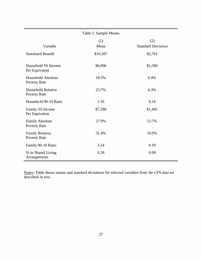
Table 1: Sample Means

Variable

(1)

Mean

(2)

Standard Deviation Simulated Benefit

$10,507

$2,761

Household SS Income Per Equivalent

$6,896

$1,396

Household Absolute Poverty Rate

18.5%

6.9%

Household Relative Poverty Rate

23.7%

6.3%

Household 90-10 Ratio

1.56

0.14

Family SS Income Per Equivalent

$7,288

$1,441

Family Absolute Poverty Rate

27.9%

12.7%

Family Relative Poverty Rate

31.4%

10.9%

Family 90-10 Ratio

1.54

0.19

% in Shared Living Arrangements

0.28

0.09

Notes: Table shows means and standard deviations for selected variables from the CPS data set described in text.

28

Table 2: Estimation Results for Full Sample

(1)

OLS

(2)

IV

(3)

IV, with controls

(4)

Log IV

(5)

Log IV,

with controls

A. Household Level Absolute Poverty

-.028 (.002)

-.035 (.003)

-.031 (.003)

-.752 (.146)

-.722

(0.165) Relative Poverty

-.028 (.002)

-.034 (.003)

-.035 (.004)

-1.025 (.127)

-1.155 (.151)

90-10 Ratio

-.055 (.009)

-.083 (.013)

- 035 (.016)

-.478 (.072)

-.221 (.085)

B. Family Level

Absolute Poverty

-.055 (.003)

-.068 (.004)

-.057 (.004)

-1.721 (.174)

-1.383 (.176)

Relative Poverty

-.049 (.003)

-.057 (.004)

-.052 (.004)

-1.693 (.163)

-1.575 (.178)

90-10 Ratio

-.049 (.011)

-.065 (.015)

-.018 (.019)

-.286 (.104)

-.017 (.118)

Shared Living

- .036 ( .003)

-.047 (.004)

-.038 (.004)

-2.382 (.221)

-1.787 (0.211)

Notes: N = 950 for all regressions. Table shows coefficients of interest from regressions that also include the full set of age and year dummies. Standard errors are in parentheses. Regressions “with controls” also include controls for the percentage in age/year cell that are: female; white; high school graduate; some college; college graduate; advanced degree; married; divorced/separated; widowed. The IV regressions instrument with the simulated Social Security benefit described in text. First three columns are estimated in levels; remaining columns in logs.

29

Table 3: Estimation Results Restricting the Time Period to 1906-1926

(1) IV, with Controls

(2) Log IV, with

Controls

B. Household Level

Absolute Poverty

-.022 ( .004)

- 1.062 ( .243)

Relative Poverty

-.032 (.005)

-1.372 (.246)

90-10 Ratio -.016 (.022)

-.097 (.118)

A. Family Level

Absolute Poverty

-.025 (.004)

-.989 (.206)

Relative Poverty

-.030 (.005)

-1.117 (.189)

90-10 Ratio -.027 (.024)

-.158 (.137)

Shared Living -.009 (.004)

-.341 (.174)

Notes: N = 419 for all regressions. Table shows coefficients of interest from regressions that also include the full set of age and year dummies and controls for the percentage in age/year cell that are: female; white; high school graduate; some college; college graduate; advanced degree; married; divorced/separated; widowed. Standard errors are in parentheses. The regressions instrument with the simulated Social Security benefit described in text. First column estimated in levels, second in logs.

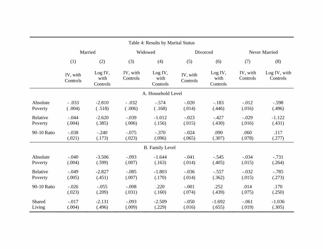
Table 4: Results by Marital Status

Married

Widowed

Divorced

Never Married

(1)

IV, with Controls

(2)

Log IV,

with Controls

(3)

IV, with Controls

(4)

Log IV,

with Controls

(5)

IV, with Controls

(6)

Log IV,

with Controls

(7)

IV, with Controls

(8)

Log IV, with

Controls

A. Household Level

Absolute Poverty

- .033 ( .004)

-2.810 ( .518)

- .032 ( .006)

-.574 ( .168)

-.020 (.014)

-.183 (.446)

-.012 (.016)

-.598 (.496)

Relative Poverty

-.044 (.004)

-2.620 (.385)

-.039 (.006)

-1.012 (.156)

-.023 (.015)

-.427 (.430)

-.029 (.016)

-1.122 (.431)

90-10 Ratio

-.038 (.021)

-.240 (.173)

-.075 (.023)

-.370 (.096)

-.024 (.065)

.090

(.307)

.060

(.078)

.117

(.277)

B. Family Level

Absolute Poverty

-.040 (.004)

-3.506 (.599)

-.093 (.007)

-1.644 (.163)

-.041 (.014)

-.545 (.405)

-.034 (.015)

-.731 (.264)

Relative Poverty

-.049 (.005)

-2.827 (.451)

-.085 (.007)

-1.803 (.170)

-.036 (.014)

-.557 (.362)

-.032 (.015)

-.785 (.273)

90-10 Ratio

-.026 (.023)

-.055 (.209)

-.008 (.031)

.220

(.160)

-.001 (.074)

.252

(.439)

.014

(.075)

.170

(.250) Shared Living

-.017 (.004)

-2.131 (.496)

-.093 (.009)

-2.509 (.229)

-.050 (.016)

-1.692 (.655)

-.061 (.019)

-1.036 (.305)

31

Notes: N = cells for married regressions (first set of two columns), 950 for widowed regressions (second set of two columns), 815 cells for widowed regressions (third set of two columns), 808 for never married regressions (last set of two columns). Table shows coefficients of interest from regressions that also include the full set of age and year dummies and controls for the percentage in age/year cell that are: female; white; high school graduate; some college; college graduate; advanced degree. Standard errors are in parentheses. The regressions instrument with the simulated Social Security benefit described in text. First column in each panel estimated in levels, second in logs.

32

% <

pov

erty

line

Figure 1: Elderly Poverty and Social Security Expenditures Over Timecalendar year

SS

Exp

endi

ture

s P

er C

apita

% < poverty line SS Expenditures Per Capita

1967 1973 1980 1984 1990 1995 2000

.103877

.298679

4328.81

8938.89

33

SS

Exp

endi

ture

s P

er C

apita

Figure 2: Absolute SS Expend and Relative SS Expend Over Timecalendar year

SS

Exp

end

/ Non

elde

rly In

com

e

SS Expenditures Per Capita SS Expend / Nonelderly Income

1967 1973 1980 1984 1990 1995 2000

4328.81

8938.89

.282708

.425825

34

% <

pov

erty

line

Figure 3: Elderly and Nonelderly Poverty Over Timecalendar year

% <

pov

line,

none

lder

ly

% < poverty line % < povline,nonelderly

1967 1973 1980 1984 1990 1995 2000

.103877

.298679

.066144

.103562

35

% <

40%

non

elde

rly

med

ian

Figure 4: Relative Povertycalendar year

% <

40%

non

eld,

non

elde

rly

% < 40% nonelderly median % < 40% noneld, nonelderly

1967 1973 1980 1984 1990 1995 2000

.180359

.291928

.097004

.154382

36

90-1

0 ra

tio

Figure 5: Income Inequalitycalendar year

90-1

0 ra

tio, n

onel

derly

90-10 ratio 90-10 ratio, nonelderly

1967 1973 1980 1984 1990 1995 2000

1.50403

1.68915

1.41483

1.67053

37

frac

tion

in s

hare

d liv

ing

arra

ng

Figure 6: Shared Living Arrangementscalendar year

1967 1973 1980 1984 1990 1995 2000

.229604

.341977

38

% <

pov

erty

line

Figure 7: Absolute Poverty,Familiescalendar year

% <

pov

line,

none

lder

ly

% < poverty line % < povline,nonelderly

1967 1973 1980 1984 1990 1995 2000

.151226

.435188

.0867

.143418

39

Figure 8: Poverty by Age Groupcalendar year

% < povline, age 65-69 % < povline, age 70-74 % < povline, age 75-79 % < povline, age 80+

1967 1973 1980 1984 1990 1995 2000

.05

.1

.15

.2

.25

.3

.35

.4

40

Figure 9: Poverty Line by Marital Statuscalendar year

% < povline, married % < povline, divorced % < povline, widowed % < povline, nev married

1967 1973 1980 1984 1990 1995 2000

.05

.1

.15

.2

.25

.3

.35

.4

41

HH

Inco

me

from

SS

Figure 10: Actual vs. Simulated Benefits by Birth Cohortyear of birth

Sim

ulat

ed B

enef

its

HH Income from SS Simulated Benefits

1885 1900 1916 1930

4493.31

7859.77

3382.33

15521.7

42

% in

Pov

erty

, HH

Figure 11: HH Poverty Rate vs. Benefits by Birth Cohortyear of birth

Sim

ulat

ed B

enef

its

% in Poverty, HH Simulated Benefits

1885 1916 1930

.089848

.352675

3382.33

15521.7

43

% in

Sha

red

Livi

ng

Figure 12: Shared Living vs. Benefits by Birth Cohortyear of birth

Sim

ulat

ed B

enef

its

% in Shared Living Simulated Benefits

1885 1916 1930

.220149

.456379

3382.33

15521.7

44