Simulink 8.3 - Release 2014a - Electronics
87
SimElectronics ® User’s Guide R2014a
-
Upload
ariana-ribeiro-lameirinhas -
Category
Documents
-
view
127 -
download
7
Transcript of Simulink 8.3 - Release 2014a - Electronics

SimElectronics®
User’s Guide
R2014a

How to Contact MathWorks
www.mathworks.com Webcomp.soft-sys.matlab Newsgroupwww.mathworks.com/contact_TS.html Technical Support
[email protected] Product enhancement [email protected] Bug [email protected] Documentation error [email protected] Order status, license renewals, [email protected] Sales, pricing, and general information
508-647-7000 (Phone)
508-647-7001 (Fax)
The MathWorks, Inc.3 Apple Hill DriveNatick, MA 01760-2098For contact information about worldwide offices, see the MathWorks Web site.
SimElectronics® User’s Guide
© COPYRIGHT 2008–2014 by The MathWorks, Inc.The software described in this document is furnished under a license agreement. The software may be usedor copied only under the terms of the license agreement. No part of this manual may be photocopied orreproduced in any form without prior written consent from The MathWorks, Inc.
FEDERAL ACQUISITION: This provision applies to all acquisitions of the Program and Documentationby, for, or through the federal government of the United States. By accepting delivery of the Programor Documentation, the government hereby agrees that this software or documentation qualifies ascommercial computer software or commercial computer software documentation as such terms are usedor defined in FAR 12.212, DFARS Part 227.72, and DFARS 252.227-7014. Accordingly, the terms andconditions of this Agreement and only those rights specified in this Agreement, shall pertain to and governthe use, modification, reproduction, release, performance, display, and disclosure of the Program andDocumentation by the federal government (or other entity acquiring for or through the federal government)and shall supersede any conflicting contractual terms or conditions. If this License fails to meet thegovernment’s needs or is inconsistent in any respect with federal procurement law, the government agreesto return the Program and Documentation, unused, to The MathWorks, Inc.
Trademarks
MATLAB and Simulink are registered trademarks of The MathWorks, Inc. Seewww.mathworks.com/trademarks for a list of additional trademarks. Other product or brandnames may be trademarks or registered trademarks of their respective holders.
Patents
MathWorks products are protected by one or more U.S. patents. Please seewww.mathworks.com/patents for more information.

Revision HistoryApril 2008 Online only New for Version 1.0 (Release 2008a+)October 2008 Online only Revised for Version 1.1 (Release 2008b)March 2009 Online only Revised for Version 1.2 (Release 2009a)September 2009 Online only Revised for Version 1.3 (Release 2009b)March 2010 Online only Revised for Version 1.4 (Release 2010a)September 2010 Online only Revised for Version 1.5 (Release 2010b)April 2011 Online only Revised for Version 1.6 (Release 2011a)September 2011 Online only Revised for Version 2.0 (Release 2011b)March 2012 Online only Revised for Version 2.1 (Release 2012a)September 2012 Online only Revised for Version 2.2 (Release 2012b)March 2013 Online only Revised for Version 2.3 (Release 2013a)September 2013 Online only Revised for Version 2.4 (Release 2013b)March 2014 Online only Revised for Version 2.5 (Release 2014a)


Contents
Getting Started
1SimElectronics Product Description . . . . . . . . . . . . . . . . 1-2Key Features . . . . . . . . . . . . . . . . . . . . . . . . . . . . . . . . . . . . . 1-2
SimElectronics Assumptions and Limitations . . . . . . . . 1-3
Modeling Physical Networks with SimElectronicsBlocks . . . . . . . . . . . . . . . . . . . . . . . . . . . . . . . . . . . . . . . . . . 1-4
Required and Related Products . . . . . . . . . . . . . . . . . . . . . 1-5Product Requirements . . . . . . . . . . . . . . . . . . . . . . . . . . . . . 1-5Other Related Products . . . . . . . . . . . . . . . . . . . . . . . . . . . . 1-5
SimElectronics Block Libraries . . . . . . . . . . . . . . . . . . . . . 1-6Overview of SimElectronics Libraries . . . . . . . . . . . . . . . . . 1-6Opening SimElectronics Libraries . . . . . . . . . . . . . . . . . . . . 1-6
Modeling Electronic and ElectromechanicalSystems . . . . . . . . . . . . . . . . . . . . . . . . . . . . . . . . . . . . . . . . 1-10
Essential Electronic Modeling Techniques . . . . . . . . . . . 1-11Overview of Modeling Rules . . . . . . . . . . . . . . . . . . . . . . . . . 1-11Required Blocks . . . . . . . . . . . . . . . . . . . . . . . . . . . . . . . . . . . 1-13Creating a New Model . . . . . . . . . . . . . . . . . . . . . . . . . . . . . 1-13Modeling Instantaneous Events . . . . . . . . . . . . . . . . . . . . . . 1-13Using Simulink Blocks to Model Physical Components . . . 1-14
Simulating an Electronic System . . . . . . . . . . . . . . . . . . . . 1-16Selecting a Solver . . . . . . . . . . . . . . . . . . . . . . . . . . . . . . . . . 1-16Specifying Simulation Accuracy/Speed Tradeoff . . . . . . . . . 1-16Avoiding Simulation Issues . . . . . . . . . . . . . . . . . . . . . . . . . 1-17Running a Time-Domain Simulation . . . . . . . . . . . . . . . . . . 1-18Running a Small-Signal Frequency-Domain Analysis . . . . 1-18
v

DC Motor Model . . . . . . . . . . . . . . . . . . . . . . . . . . . . . . . . . . . 1-19Overview of DC Motor Example . . . . . . . . . . . . . . . . . . . . . . 1-19Selecting Blocks to Represent System Components . . . . . . 1-19Building the Model . . . . . . . . . . . . . . . . . . . . . . . . . . . . . . . . 1-20Specifying Model Parameters . . . . . . . . . . . . . . . . . . . . . . . . 1-22Configuring the Solver Parameters . . . . . . . . . . . . . . . . . . . 1-29Running the Simulation and Analyzing the Results . . . . . 1-30
Triangle Wave Generator Model . . . . . . . . . . . . . . . . . . . . 1-33Overview of Triangle Wave Generator Example . . . . . . . . . 1-33Selecting Blocks to Represent System Components . . . . . . 1-33Building the Model . . . . . . . . . . . . . . . . . . . . . . . . . . . . . . . . 1-35Specifying Model Parameters . . . . . . . . . . . . . . . . . . . . . . . . 1-37Configuring the Solver Parameters . . . . . . . . . . . . . . . . . . . 1-45Running the Simulation and Analyzing the Results . . . . . 1-46
Modeling an Electronic System
2Parameterizing Blocks from Datasheets . . . . . . . . . . . . . 2-2
Parameterize a Piecewise Linear Diode Model . . . . . . . 2-4
Parameterize an Exponential Diode from aDatasheet . . . . . . . . . . . . . . . . . . . . . . . . . . . . . . . . . . . . . . . 2-7
Parameterize an Exponential Diode from SPICENetlist . . . . . . . . . . . . . . . . . . . . . . . . . . . . . . . . . . . . . . . . . . 2-11
Parameterize an Op-Amp from a Datasheet . . . . . . . . . . 2-15
Additional Parameterization Workflows . . . . . . . . . . . . . 2-17Validation Using Data from SPICE Tool . . . . . . . . . . . . . . . 2-17Parameter Tuning Against External Data . . . . . . . . . . . . . 2-17Building an Equivalent Model of a SPICE Netlist . . . . . . . 2-17
Selecting the Output Model for Logic Blocks . . . . . . . . . 2-18
vi Contents
Available Output Models . . . . . . . . . . . . . . . . . . . . . . . . . . . 2-18Quadratic Model Output and Parameters . . . . . . . . . . . . . . 2-19
Simulating Thermal Effects in Semiconductors . . . . . . 2-22Using the Thermal Ports . . . . . . . . . . . . . . . . . . . . . . . . . . . 2-22Thermal Model for Semiconductor Blocks . . . . . . . . . . . . . . 2-24Thermal Mass Parameterization . . . . . . . . . . . . . . . . . . . . . 2-25Electrical Behavior Depending on Temperature . . . . . . . . . 2-26Improving Numerical Performance . . . . . . . . . . . . . . . . . . . 2-26
Simulating Thermal Effects in Rotational andTranslational Actuators . . . . . . . . . . . . . . . . . . . . . . . . . . 2-28Using the Thermal Ports . . . . . . . . . . . . . . . . . . . . . . . . . . . 2-28Thermal Model for Actuator Blocks . . . . . . . . . . . . . . . . . . . 2-30
vii

viii Contents

1
Getting Started
• “SimElectronics Product Description” on page 1-2
• “SimElectronics Assumptions and Limitations” on page 1-3
• “Modeling Physical Networks with SimElectronics Blocks” on page 1-4
• “Required and Related Products” on page 1-5
• “SimElectronics Block Libraries” on page 1-6
• “Modeling Electronic and Electromechanical Systems” on page 1-10
• “Essential Electronic Modeling Techniques” on page 1-11
• “Simulating an Electronic System” on page 1-16
• “DC Motor Model” on page 1-19
• “Triangle Wave Generator Model” on page 1-33

1 Getting Started
SimElectronics Product DescriptionModel and simulate electronic and mechatronic systems
SimElectronics® provides component libraries for modeling and simulatingelectronic and mechatronic systems. The libraries include models ofsemiconductors, motors, drives, sensors, and actuators. You can use thesecomponents to develop electromechanical actuation systems and to buildbehavioral models for evaluating analog circuit architectures in Simulink®.
SimElectronics models can be used to develop control algorithms in electronicand mechatronic systems, including vehicle body electronics, aircraftservomechanisms, and audio power amplifiers. The semiconductor modelsinclude nonlinear and dynamic temperature effects, enabling you to selectcomponents in amplifiers, analog-to-digital converters, phase-locked loops,and other circuits. You can parameterize your models using MATLAB®
variables and expressions. You can add mechanical, hydraulic, pneumatic,and other components to a model using Simscape™ and test them in a singlesimulation environment. To deploy models to other simulation environments,including hardware-in-the-loop (HIL) systems, SimElectronics supportsC-code generation.
Key Features
• Libraries of electronic and electromechanical components with physicalconnections, including sensors, semiconductors, and actuators
• Parameterization options, enabling key parameter values to be entereddirectly from industry data sheets
• Semiconductor and motor models with temperature-dependent behaviorand configurable thermal ports
• Ideal and nonideal model variants, enabling adjustment of model fidelity
• Ability to extend component libraries using the Simscape language
• Access to linearization and steady-state calculation capabilities in Simscape
• Support for C-code generation
1-2
SimElectronics® Assumptions and Limitations
SimElectronics Assumptions and LimitationsSimElectronics contains blocks that let you model electronic and mechatronicsystems at a speed and level of fidelity that is appropriate for system-levelanalysis. The blocks let you perform tradeoff analyses to optimize systemdesign, for example, by testing various algorithms with different circuitimplementations. The library contains blocks that use either high-level ormore detailed models to simulate components. SimElectronics does not havethe capability to:
• Model large circuits with dozens of analog components, such as a completetransceiver.
• Perform either layout (physical design) tasks, or the associatedimplementation tasks such as layout versus schematic (LVS), design rulechecking (DRC), parasitic extraction, and back annotation.
• Model 3-D parasitic effects that are typically important for high-frequencyapplications.
For these types of requirements, you must use an EDA package specificallydesigned for the implementation of analog circuits.
Another MathWorks® product, SimPowerSystems™ software, is better suitedfor power system networks where:
• The underlying equations are predominantly linear (e.g., transmissionlines and linear machine models).
• Three-phase motors and generators are used.
SimPowerSystems has blocks and solvers specifically designed for thesetypes of applications.
1-3
1 Getting Started
Modeling Physical Networks with SimElectronics BlocksSimElectronics is part of the Simulink Physical Modeling family. Modelsusing SimElectronics are essentially Simscape block diagrams. To build asystem-level model with electrical blocks, use a combination of SimElectronicsblocks and other Simscape and Simulink blocks. You can connectSimElectronics blocks directly to Simscape blocks. You can connect Simulinkblocks through the Simulink-PS Converter and PS-Simulink Converter blocksfrom the Simscape Utilities library. These blocks convert electrical signalsto and from Simulink mathematical signals. For more information aboutconnecting different types of blocks, see “Connector Ports and ConnectionLines” and “Connecting Simscape Diagrams to Simulink Sources and Scopes”in the Simscape documentation.
For more information about basic principles to follow when building anelectrical model with SimElectronics, see “Basic Principles of ModelingPhysical Networks” in the Simscape documentation.
1-4
Required and Related Products
Required and Related Products
Product RequirementsSimElectronics software is an extension of Simscape product, expanding itscapabilities to model and simulate electronic and electromechanical elementsand devices.
SimElectronics software requires these products:
• MATLAB
• Simulink
• Simscape
Other Related ProductsThe SimElectronics product page at the MathWorks Web site lists thetoolboxes and blocksets that extend the capabilities of MATLAB andSimulink. These products can enhance your use of SimElectronics software invarious applications.
For more information about MathWorks software products, see:
• The online documentation for that product if it is installed
• The MathWorks Web site at www.mathworks.com
1-5
1 Getting Started
SimElectronics Block Libraries
In this section...
“Overview of SimElectronics Libraries” on page 1-6
“Opening SimElectronics Libraries” on page 1-6
Overview of SimElectronics LibrariesSimElectronics libraries provide blocks for modeling electromechanical andelectrical systems within the Simulink environment. You can also createcustom components either by combining SimElectronics components asSimulink subsystems, or by using the Simscape language.
Note SimElectronics follows the standard Simulink conventions where blockinputs and outputs are called ports. In SimElectronics, each port representsa single electrical terminal.
A SimElectronics model can contain blocks from the standard SimElectronicslibrary, from the Simscape Foundation and Utilities libraries, or from acustom library you create, using the Simscape language, based on theSimscape Foundation electrical domain. A model can also include blocks fromother Simscape add-on products, as well as Simulink blocks.
Opening SimElectronics LibrariesThere are two ways to access SimElectronics blocks:
• “Using the Simulink Library Browser to Access the Block Libraries” onpage 1-7
• “Using the Command Prompt to Access the Block Libraries” on page 1-8
1-6

SimElectronics® Block Libraries
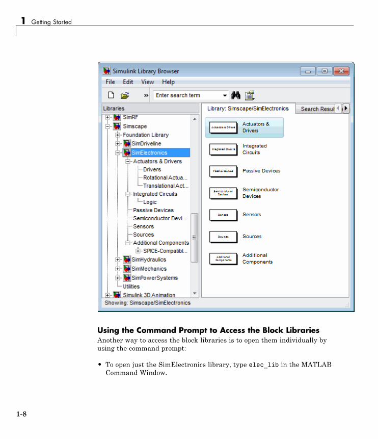
Using the Simulink Library Browser to Access the BlockLibrariesYou can access the blocks through the Simulink Library Browser. To displaythe Library Browser, click the Library Browser button in the toolbar of theMATLAB desktop or Simulink model window:
Alternatively, you can type simulink in the MATLAB Command Window.Then expand the Simscape entry in the contents tree.
1-7
1 Getting Started
Using the Command Prompt to Access the Block LibrariesAnother way to access the block libraries is to open them individually byusing the command prompt:
• To open just the SimElectronics library, type elec_lib in the MATLABCommand Window.
1-8
SimElectronics® Block Libraries
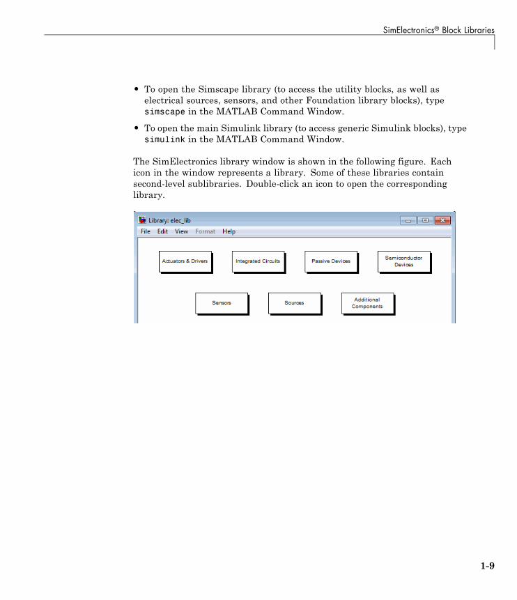
• To open the Simscape library (to access the utility blocks, as well aselectrical sources, sensors, and other Foundation library blocks), typesimscape in the MATLAB Command Window.
• To open the main Simulink library (to access generic Simulink blocks), typesimulink in the MATLAB Command Window.
The SimElectronics library window is shown in the following figure. Eachicon in the window represents a library. Some of these libraries containsecond-level sublibraries. Double-click an icon to open the correspondinglibrary.
1-9

1 Getting Started
Modeling Electronic and Electromechanical SystemsWhen you model and analyze an electronic or electromechanical system usingSimElectronics software, your workflow might include the following tasks:
1 Create a Simulink model that includes electronic or electromechanicalcomponents.
In the majority of applications, it is most natural to model the physicalsystem using Simscape and SimElectronics blocks, and then develop thecontroller or signal processing algorithm in Simulink.
For more information about modeling the physical system, see “EssentialElectronic Modeling Techniques” on page 1-11.
2 Define component data by specifying electrical or mechanical propertiesas defined on a datasheet.
For more information about parameterizing blocks, see “ParameterizingBlocks from Datasheets” on page 2-2.
3 Configure the solver options.
For more information about the settings that most affect the solution ofa physical system, see “Setting Up Solvers for Physical Models” in theSimscape documentation..
4 Run the simulation.
For more information on how to perform time-domain simulation of anelectronic system, see “Simulating an Electronic System” on page 1-16.
1-10
Essential Electronic Modeling Techniques
Essential Electronic Modeling Techniques
In this section...
“Overview of Modeling Rules” on page 1-11
“Required Blocks” on page 1-13
“Creating a New Model” on page 1-13
“Modeling Instantaneous Events” on page 1-13
“Using Simulink Blocks to Model Physical Components” on page 1-14
Overview of Modeling RulesSimElectronics models are essentially Simscape block diagrams. Tobuild a system-level model with electrical blocks, use a combination ofSimElectronics blocks and other Simscape and Simulink blocks. You canconnect SimElectronics blocks directly to Simscape blocks. You can connectSimulink blocks through the Simulink-PS Converter and PS-SimulinkConverter blocks from the Simscape Utilities library. These blocks convertelectrical signals to and from Simulink mathematical signals.
The rules that you must follow when building an electronic orelectromechanical model are described in “Basic Principles of ModelingPhysical Networks” in the Simscape documentation. This section brieflyreviews these rules.
• SimElectronics blocks, in general, feature Conserving ports and PhysicalSignal inports and outports .
• There are two main types of Physical Conserving ports used inSimElectronics blocks: electrical and mechanical rotational. Each type hasspecific Through and Across variables associated with it.
• You can connect Conserving ports only to other Conserving ports of thesame type.
• The Physical connection lines that connect Conserving ports together arenondirectional lines that carry physical variables (Across and Throughvariables, as described above) rather than signals. You cannot connectPhysical lines to Simulink ports or to Physical Signal ports.
1-11

1 Getting Started
• Two directly connected Conserving ports must have the same values for alltheir Across variables (such as voltage or angular velocity).
• You can branch Physical connection lines. When you do so, componentsdirectly connected with one another continue to share the same Acrossvariables. Any Through variable (such as current or torque) transferredalong the Physical connection line is divided among the multiplecomponents connected by the branches. How the Through variable isdivided is determined by the system dynamics.
For each Through variable, the sum of all its values flowing into a branchpoint equals the sum of all its values flowing out.
• You can connect Physical Signal ports to other Physical Signal ports withregular connection lines, similar to Simulink signal connections. Theseconnection lines carry physical signals between SimElectronics blocks.
• You can connect Physical Signal ports to Simulink ports through specialconverter blocks. Use the Simulink-PS Converter block to connect Simulinkoutports to Physical Signal inports. Use the PS-Simulink Converter blockto connect Physical Signal outports to Simulink inports.
• Unlike Simulink signals, which are essentially unitless, Physical Signalscan have units associated with them. SimElectronics block dialogs let youspecify the units along with the parameter values, where appropriate. Usethe converter blocks to associate units with an input signal and to specifythe desired output signal units.
For examples of applying these rules when creating an actualelectromechanical model, see “DC Motor Model” on page 1-19.
MathWorks recommends that you build, simulate, and test your modelincrementally. Start with an idealized, simplified model of your system,simulate it, verify that it works the way you expected. Then incrementallymake your model more realistic, factoring in effects such as motor shaftcompliance, hard stops, and the other things that describe real-worldphenomena. Simulate and test your model at every incremental step. Usesubsystems to capture the model hierarchy, and simulate and test yoursubsystems separately before testing the whole model configuration. Thisapproach helps you keep your models well organized and makes it easierto troubleshoot them.
1-12

Essential Electronic Modeling Techniques
Required BlocksEach topologically distinct physical network in a diagram requires exactlyone Solver Configuration block, found in the Simscape Utilities library. TheSolver Configuration block specifies global environment information forsimulation and provides parameters for the solver that your model needsbefore you can begin simulation. For more information, see the SolverConfiguration block reference page.
Each electrical network requires an Electrical Reference block. Thisblock establishes the electrical ground for the circuit. Networks withelectromechanical blocks also require a Mechanical Rotational Referenceblock. For more information about using reference blocks, see “GroundingRules” in the Simscape documentation.
Creating a New ModelAn easy way to start a new SimElectronics model, prepopulated with therequired blocks, is to use the Simscape function ssc_new with a domaintype of electrical and the desired solver type. For more information, see“Creating a New Simscape Model”.
You can also use the Creating A New Circuit example (under Simscapeexamples) as a template for a new model. This example opens a simpleelectrical model, prepopulated with some useful blocks, and also opensan Electrical Starter Palette, which contains links to the most often usedelectrical components. Open the example by typing ssc_new_elec in theMATLAB Command Window and use File > Save As to save the examplemodel under the desired name. Then delete the unwanted blocks and add newones from the Electrical Starter Palette and from the block libraries.
Modeling Instantaneous EventsWhen working with SimElectronics software, your model may includeSimulink blocks that create instantaneous changes to the physical systeminputs through the Simulink-PS Converter block, such as those associatedwith events or discrete sampling. When you build this type of model, makesure the corresponding zero crossings are generated.
Many blocks in the Simulink library generate these zero crossings bydefault. For example, the Pulse Generator block produces a discrete-time
1-13

1 Getting Started
output by default, and generates the corresponding zero crossings. To modelinstantaneous events, select Use local settings or Enable all for theZero crossing control option under the model’s Solver ConfigurationParameters to generate zero crossings. For more information about zerocrossing control, see “Zero-crossing control” in the Simulink documentation.
Using Simulink Blocks to Model Physical ComponentsTo run a fast simulation that approximates the behavior of the physicalcomponents in a system, you may want to use Simulink blocks to model of oneor more physical components.
The Modeling an Integrated Circuit example uses Simulink to model aphysical component. The Behavioral Model part of the example includesa subsystem, comprised of Simulink blocks, that implements the customintegrated circuit behavior.
The subsystem is shown in the following illustration.
1-14

Essential Electronic Modeling Techniques
The Simulink Logical Operator block implements the behavioral model of thetwo-input NOR gate. Using Simulink in this manner introduces algebraicloops, unless you place a lag somewhere between the physical signal inputsand outputs. In this case, a first-order lag is included in the Propagation Delaysubsystem to represent the delay due to gate capacitances. For applicationswhere no lag is required, use blocks from the Physical Signals sublibrary inthe Simscape Foundation Library to implement the desired functionality.
1-15
1 Getting Started
Simulating an Electronic System
In this section...
“Selecting a Solver” on page 1-16
“Specifying Simulation Accuracy/Speed Tradeoff” on page 1-16
“Avoiding Simulation Issues” on page 1-17
“Running a Time-Domain Simulation” on page 1-18
“Running a Small-Signal Frequency-Domain Analysis” on page 1-18
Selecting a SolverSimElectronics software supports all of the continuous-time solvers thatSimscape supports. For more information, see “Setting Up Solvers forPhysical Models” in the Simscape documentation.
You can select any of the supported solvers for running a SimElectronicssimulation. The variable-step solvers, ode23t and ode15s, are recommendedfor most applications because they run faster and work better for systemswith a range of both fast and slow dynamics. The ode23t solver is closest tothe solver that SPICE traditionally uses.
To use Simulink Coder™ software to generate standalone C or C++ code fromyour model, you must use the ode14x solver. For more information about codegeneration, see “Code Generation” in the Simscape documentation.
Specifying Simulation Accuracy/Speed TradeoffTo trade off accuracy and simulation time, adjust one or more of the followingparameters:
• Relative tolerance (in the Configuration Parameters dialog box)
• Absolute tolerance (in the Configuration Parameters dialog box)
• Max step size (in the Configuration Parameters dialog box)
• Constraint Residual Tolerance (in the Solver Configuration blockdialog box)
1-16
Simulating an Electronic System
In most cases, the default tolerance values produce accurate results withoutsacrificing unnecessary simulation time. The parameter value that is mostlikely to be inappropriate for your simulation is Max step size, because thedefault value, auto, depends on the simulation start and stop times ratherthan on the amount by which the signals are changing during the simulation.If you are concerned about the solver missing significant behavior, change theparameter to prevent the solver from taking too large a step.
The Simulink documentation describes the following parameters in moredetail and provides tips on how to adjust them:
• “Relative tolerance”
• “Absolute tolerance”
• “Max step size”
The Solver Configuration block reference page in the Simscape documentationexplains when to adjust the Constraint Residual Tolerance parametervalue.
Avoiding Simulation IssuesIf you experience a simulation issue, first read “Troubleshooting SimulationErrors” in the Simscape documentation to learn about general troubleshootingtechniques.
Note SimElectronics software does not have the ability to model large circuitswith dozens of analog components. If you encounter convergence issues whentrying to simulate a model with more than a few tens of transistors, youmay find that the limitations of SimElectronics software prevent you fromachieving convergence with any set of simulation parameter values.
There are a few techniques you can apply to any SimElectronics model toovercome simulation issues:
• Add parasitic capacitors and/or resistors (specifically, junction capacitanceand ohmic resistance) to the circuit to avoid numerical issues. The AstableOscillator example uses these devices.
1-17

1 Getting Started
• Adjust the current and voltage sources so they start at zero and ramp up totheir final values rather than starting at nonzero values.
“Modeling Instantaneous Events” on page 1-13 and “Using Simulink Blocks toModel Physical Components” on page 1-14 describe how to avoid simulationerrors in the presence of specific SimElectronics model configurations.
Running a Time-Domain SimulationWhen you run a time-domain simulation, SimElectronics software uses theSimscape solver to analyze the physical system in the Simulink environment.For more information, see “How Simscape Simulation Works” in the Simscapedocumentation.
Running a Small-Signal Frequency-Domain AnalysisYou can perform small-signal analysis for Simscape and SimElectronicsmodels using linearization capabilities of Simulink software. For moreinformation, see “Linearize an Electronic Circuit” in the Simscapedocumentation.
1-18

DC Motor Model
DC Motor Model
In this section...
“Overview of DC Motor Example” on page 1-19
“Selecting Blocks to Represent System Components” on page 1-19
“Building the Model” on page 1-20
“Specifying Model Parameters” on page 1-22
“Configuring the Solver Parameters” on page 1-29
“Running the Simulation and Analyzing the Results” on page 1-30
Overview of DC Motor ExampleIn this example, you model a DC motor driven by a constant input signal thatapproximates a pulse-width modulated signal and look at the current androtational motion at the motor output.
To see the completed model, open the Controlled DC Motor example.
Selecting Blocks to Represent System ComponentsSelect the blocks to represent the input signal, the DC motor, and the motoroutput displays.
The following table describes the role of the blocks that represent the systemcomponents.
Block Description
SolverConfiguration
Defines solver settings that apply to all physicalmodeling blocks.
DC Voltage Source Generates a DC signal.
Controlled PWMVoltage
Generates the signal that approximates apulse-width modulated motor input signal.
H-Bridge Drives the DC motor.
1-19

1 Getting Started
Block Description
Current Sensor Converts the electrical current that drives the motorinto a physical signal proportional to the current.
Ideal RotationalMotion Sensor
Converts the rotational motion of the motor into aphysical signal proportional to the motion.
DC Motor Converts input electrical signal into mechanicalmotion.
PS-SimulinkConverter
Converts the input physical signal to a Simulinksignal.
Scope Displays motor current and rotational motion.
ElectricalReference
Provides the electrical ground.
MechanicalRotationalReference
Provides the mechanical ground.
Building the ModelCreate a Simulink model, add blocks to the model, and connect the blocks.
1 Create a new model.
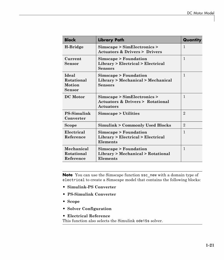
2 Add to the model the blocks listed in the following table. The Librarycolumn of the table specifies the hierarchical path to each block.
Block Library Path Quantity
SolverConfiguration
Simscape > Utilities 1
DC VoltageSource
Simscape > FoundationLibrary > Electrical > ElectricalSources
1
ControlledPWM Voltage
Simscape > SimElectronics >Actuators & Drivers > Drivers
1
1-20
DC Motor Model
Block Library Path Quantity
H-Bridge Simscape > SimElectronics >Actuators & Drivers > Drivers
1
CurrentSensor
Simscape > FoundationLibrary > Electrical > ElectricalSensors
1
IdealRotationalMotionSensor
Simscape > FoundationLibrary > Mechanical > MechanicalSensors
1
DC Motor Simscape > SimElectronics >Actuators & Drivers > RotationalActuators
1
PS-SimulinkConverter
Simscape > Utilities 2
Scope Simulink > Commonly Used Blocks 2
ElectricalReference
Simscape > FoundationLibrary > Electrical > ElectricalElements
1
MechanicalRotationalReference
Simscape > FoundationLibrary > Mechanical > RotationalElements
1
Note You can use the Simscape function ssc_new with a domain type ofelectrical to create a Simscape model that contains the following blocks:
• Simulink-PS Converter
• PS-Simulink Converter
• Scope
• Solver Configuration
• Electrical ReferenceThis function also selects the Simulink ode15s solver.
1-21
1 Getting Started
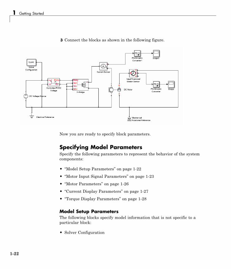
3 Connect the blocks as shown in the following figure.
Now you are ready to specify block parameters.
Specifying Model ParametersSpecify the following parameters to represent the behavior of the systemcomponents:
• “Model Setup Parameters” on page 1-22
• “Motor Input Signal Parameters” on page 1-23
• “Motor Parameters” on page 1-26
• “Current Display Parameters” on page 1-27
• “Torque Display Parameters” on page 1-28
Model Setup ParametersThe following blocks specify model information that is not specific to aparticular block:
• Solver Configuration
1-22

DC Motor Model
• Electrical Reference
• Mechanical Rotational Reference
As with Simscape models, you must include a Solver Configuration blockin each topologically distinct physical network. This example has a singlephysical network, so use one Solver Configuration block with the defaultparameter values.
You must include an Electrical Reference block in each SimElectronicsnetwork. You must include a Mechanical Rotational Reference block in eachnetwork that includes electromechanical blocks. These blocks do not haveany parameters.
For more information about using reference blocks, see “Grounding Rules” inthe Simscape documentation.
Motor Input Signal ParametersYou generate the motor input signal using three blocks:
• The DC Voltage Source block generates a constant signal.
• The Controlled PWM Voltage block generates a pulse-width modulatedsignal.
• The H-Bridge block drives the motor.
In this example, all input ports of the H-Bridge block except the PWM portare connected to ground. As a result, the H-Bridge block behaves as follows:
• When the motor is on, the H-Bridge block connects the motor terminalsto the power supply.
• When the motor is off, the H-Bridge block acts as a freewheeling diode tomaintain the motor current.
In this example, you simulate the motor with a constant current whose valueis the average value of the PWM signal. By using this type of signal, you setup a fast simulation that estimates the motor behavior.
1 Set the DC Voltage Source block parameters as follows:
1-23
1 Getting Started
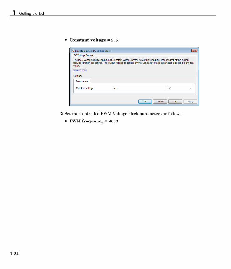
• Constant voltage = 2.5
2 Set the Controlled PWM Voltage block parameters as follows:
• PWM frequency = 4000
1-24
DC Motor Model
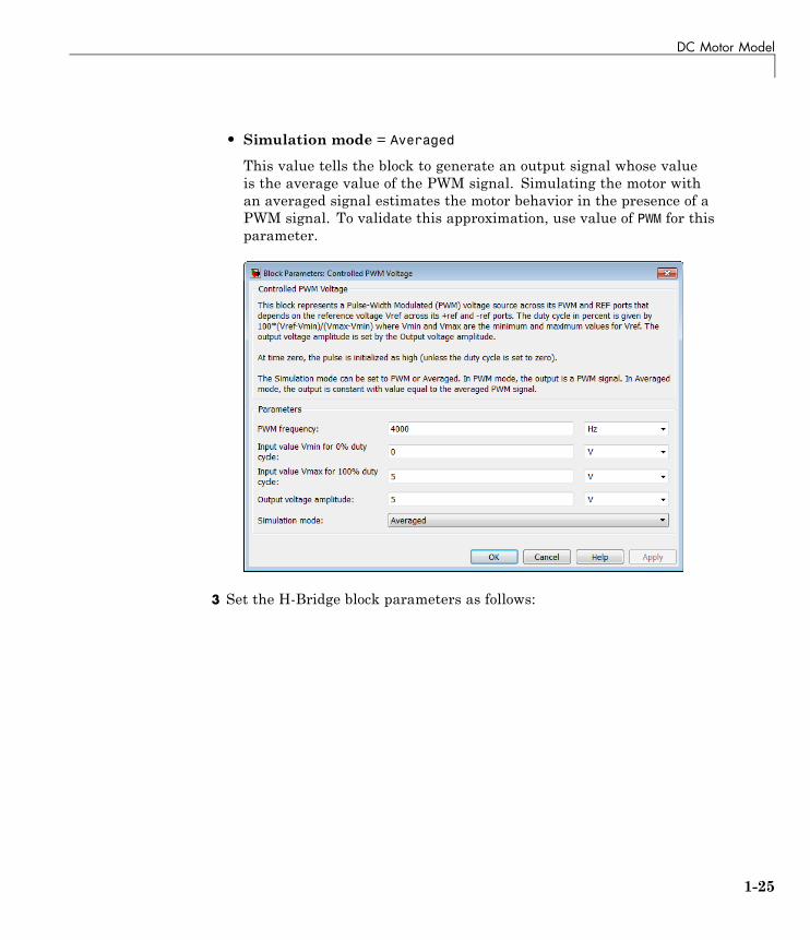
• Simulation mode = Averaged
This value tells the block to generate an output signal whose valueis the average value of the PWM signal. Simulating the motor withan averaged signal estimates the motor behavior in the presence of aPWM signal. To validate this approximation, use value of PWM for thisparameter.
3 Set the H-Bridge block parameters as follows:
1-25

1 Getting Started
• Simulation mode = Averaged
This value tells the block to generate an output signal whose valueis the average value of the PWM signal. Simulating the motor withan averaged signal estimates the motor behavior in the presence of aPWM signal. To validate this approximation, use value of PWM for thisparameter.
Motor ParametersConfigure the block that models the motor.
Set the Motor block parameters as follows, leaving the unit settings at theirdefault values where applicable:
• Electrical Torque tab:
- Model parameterization = By rated power, rated speed &no-load speed
1-26

DC Motor Model
- Armature inductance = 0.01
- No-load speed = 4000
- Rated speed (at rated load) = 2500
- Rated load (mechanical power) = 10
- Rated DC supply voltage = 12
• Mechanical tab:
- Rotor inertia = 2000
- Rotor damping = 1e-06
Current Display ParametersSpecify the parameters of the blocks that create the motor current display:
• Current Sensor block
• PS-Simulink Converter1 block
• Scope1 block
Of the three blocks, only the PS-Simulink Converter1 block has parameters.Set the PS-Simulink Converter1 block Output signal unit parameter to A toindicate that the block input signal has units of amperes.
1-27

1 Getting Started
Torque Display ParametersSpecify the parameters of the blocks that create the motor torque display:
• Ideal Rotational Motion Sensor block
• PS-Simulink Converter block
• Scope block
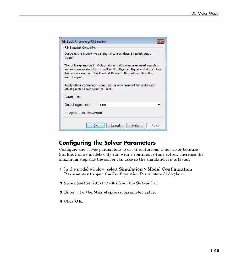
Of the three blocks, only the PS-Simulink Converter block has parametersyou need to configure for this example. Set the PS-Simulink Converter blockOutput signal unit parameter to rpm to indicate that the block input signalhas units of revolutions per minute.
Note You must type this parameter value. It is not available in thedrop-down list.
1-28
DC Motor Model
Configuring the Solver ParametersConfigure the solver parameters to use a continuous-time solver becauseSimElectronics models only run with a continuous-time solver. Increase themaximum step size the solver can take so the simulation runs faster.
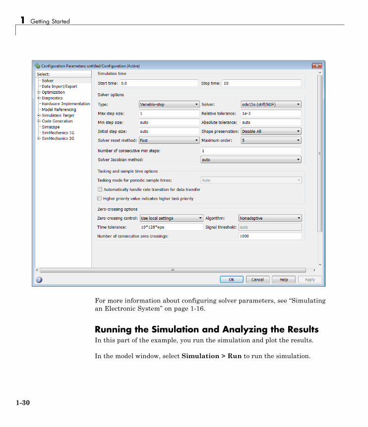
1 In the model window, select Simulation > Model ConfigurationParameters to open the Configuration Parameters dialog box.
2 Select ode15s (Stiff/NDF) from the Solver list.
3 Enter 1 for the Max step size parameter value.
4 Click OK.
1-29
1 Getting Started
For more information about configuring solver parameters, see “Simulatingan Electronic System” on page 1-16.
Running the Simulation and Analyzing the ResultsIn this part of the example, you run the simulation and plot the results.
In the model window, select Simulation > Run to run the simulation.
1-30
DC Motor Model
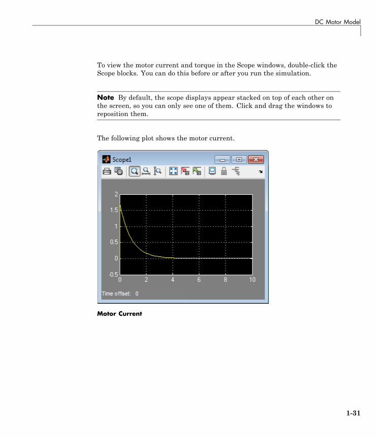
To view the motor current and torque in the Scope windows, double-click theScope blocks. You can do this before or after you run the simulation.
Note By default, the scope displays appear stacked on top of each other onthe screen, so you can only see one of them. Click and drag the windows toreposition them.
The following plot shows the motor current.
Motor Current
1-31
1 Getting Started
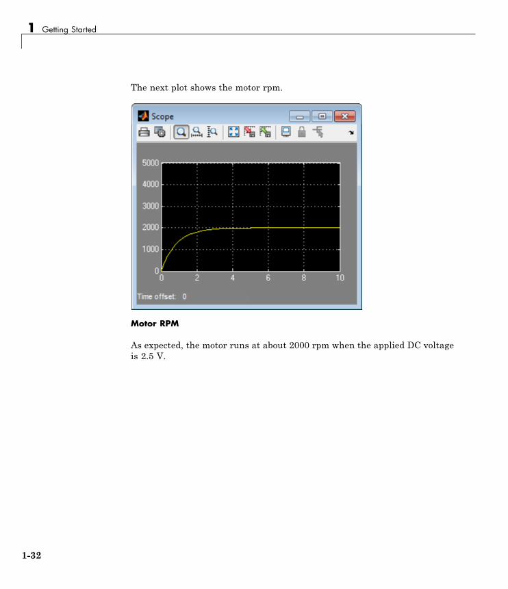
The next plot shows the motor rpm.
Motor RPM
As expected, the motor runs at about 2000 rpm when the applied DC voltageis 2.5 V.
1-32
Triangle Wave Generator Model
Triangle Wave Generator Model
In this section...
“Overview of Triangle Wave Generator Example” on page 1-33
“Selecting Blocks to Represent System Components” on page 1-33
“Building the Model” on page 1-35
“Specifying Model Parameters” on page 1-37
“Configuring the Solver Parameters” on page 1-45
“Running the Simulation and Analyzing the Results” on page 1-46
Overview of Triangle Wave Generator ExampleIn this example, you model a triangle wave generator using SimElectronicselectrical blocks and custom SimElectronics electrical blocks, and then look atthe voltage at the wave generator output.
You use a classic circuit configuration consisting of an integrator and anoninverting amplifier to generate the triangle wave, and use datasheets tospecify block parameters. For more information, see “Parameterizing Blocksfrom Datasheets” on page 2-2.
To see the completed model, open the Triangle Wave Generator example.
Selecting Blocks to Represent System ComponentsFirst, you select the blocks to represent the input signal, the triangle wavegenerator, and the output signal display.
You model the triangle wave generator with a set of physical blocks bracketedby a Simulink-PS Converter block and a PS-Simulink Converter block. Thewave generator consists of:
• Two operational amplifier blocks
• Resistors and a capacitor that work with the operational amplifiers tocreate the integrator and noninverting amplifier
1-33
1 Getting Started
• Simulink-PS Converter and PS-Simulink Converter blocks. The function ofthe Simulink-PS Converter and PS-Simulink Converter blocks is to bridgethe physical part of the model, which uses physical signals, and the rest ofthe model, which uses unitless Simulink signals.
You have a manufacturer datasheet for the two operational amplifiers youwant to model. Later in the example, you use the datasheet to parameterizethe SimElectronics Band-Limited Op-Amp block.
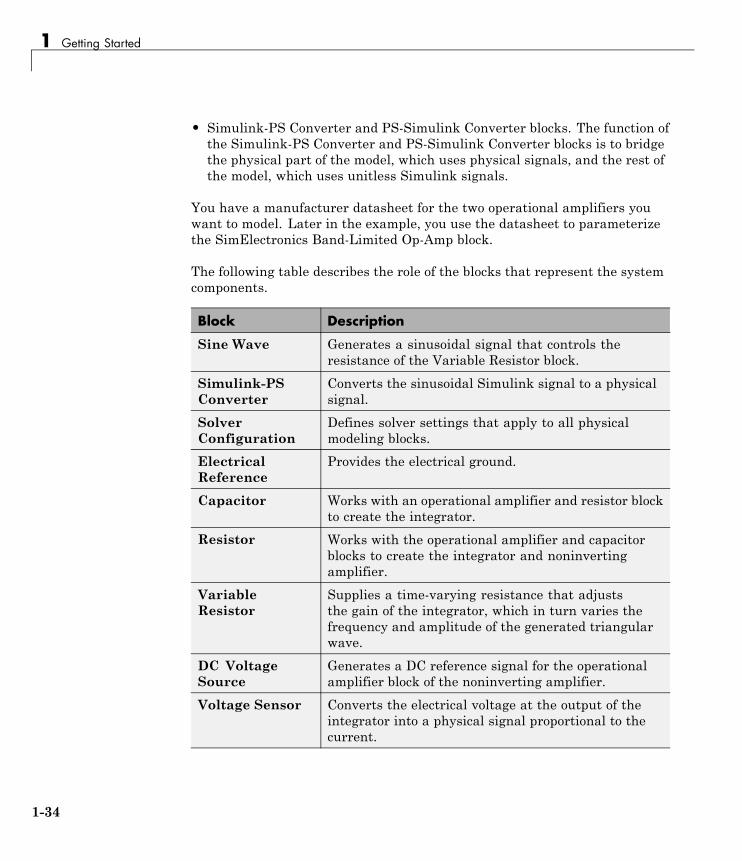
The following table describes the role of the blocks that represent the systemcomponents.
Block Description
Sine Wave Generates a sinusoidal signal that controls theresistance of the Variable Resistor block.
Simulink-PSConverter
Converts the sinusoidal Simulink signal to a physicalsignal.
SolverConfiguration
Defines solver settings that apply to all physicalmodeling blocks.
ElectricalReference
Provides the electrical ground.
Capacitor Works with an operational amplifier and resistor blockto create the integrator.
Resistor Works with the operational amplifier and capacitorblocks to create the integrator and noninvertingamplifier.
VariableResistor
Supplies a time-varying resistance that adjuststhe gain of the integrator, which in turn varies thefrequency and amplitude of the generated triangularwave.
DC VoltageSource
Generates a DC reference signal for the operationalamplifier block of the noninverting amplifier.
Voltage Sensor Converts the electrical voltage at the output of theintegrator into a physical signal proportional to thecurrent.
1-34

Triangle Wave Generator Model
Block Description
PS-SimulinkConverter
Converts the output physical signal to a Simulinksignal.
Scope Displays the triangular output wave.
Band-LimitedOp-Amp
Works with the capacitor and resistor to create anintegrator and a noninverting amplifier.
Diode Limit the output of the Band-Limited Op-Amp block,to make the output waveform independent of supplyvoltage.
Building the ModelCreate a Simulink model, add blocks to the model, and connect the blocks.
1 Create a new model.
2 Add to the model the blocks listed in the following table. The Library Pathcolumn of the table specifies the hierarchical path to each block.
Block Library Path Quantity
Sine Wave Simulink > Sources 1
Simulink-PSConverter
Simscape > Utilities 1
SolverConfiguration
Simscape > Utilities 1
ElectricalReference
Simscape > FoundationLibrary > Electrical > ElectricalElements
1
Capacitor Simscape > FoundationLibrary > Electrical > ElectricalElements
1
Resistor Simscape > FoundationLibrary > Electrical > ElectricalElements
3
1-35

1 Getting Started
Block Library Path Quantity
VariableResistor
Simscape > FoundationLibrary > Electrical > ElectricalElements
1
DC VoltageSource
Simscape > FoundationLibrary > Electrical > ElectricalSources
1
Voltage Sensor Simscape > FoundationLibrary > Electrical > ElectricalSensors
1
PS-SimulinkConverter
Simscape > Utilities 1
Scope Simulink > Commonly Used Blocks 1
Band-LimitedOp-Amp
Simscape > SimElectronics >Integrated Circuits
2
Diode Simscape > SimElectronics >Semiconductor Devices
2
Note You can use the Simscape function ssc_new with a domain type ofelectrical to create a Simscape model that contains the following blocks:
• Simulink-PS Converter
• PS-Simulink Converter
• Scope
• Solver Configuration
• Electrical ReferenceThis function also selects the Simulink ode15s solver.
1-36

Triangle Wave Generator Model
3 Connect the blocks as shown in the following figure.
Now you are ready to specify block parameters.
Specifying Model ParametersSpecify the following parameters to represent the behavior of the systemcomponents:
• “Model Setup Parameters” on page 1-37
• “Input Signal Parameters” on page 1-38
• “Triangle Wave Generator Parameters” on page 1-40
• “Signal Display Parameters” on page 1-45
Model Setup ParametersThe following blocks specify model information that is not specific to aparticular block:
1-37
1 Getting Started
• Solver Configuration
• Electrical Reference
As with Simscape models, you must include a Solver Configuration blockin each topologically distinct physical network. This example has a singlephysical network, so use one Solver Configuration block with the defaultparameter values.
You must include an Electrical Reference block in each SimElectronicsnetwork. This block does not have any parameters.
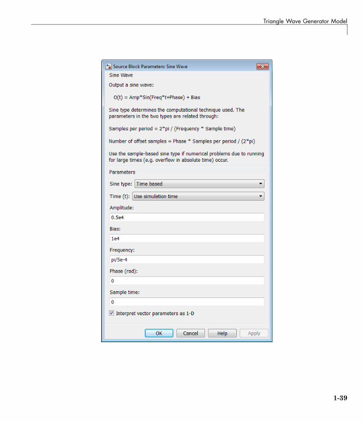
Input Signal ParametersGenerate the sinusoidal control signal using the Sine Wave block.
Set the Sine Wave block parameters as follows:
• Amplitude = 0.5e4
• Bias = 1e4
• Frequency = pi/5e-4
1-38
Triangle Wave Generator Model
1-39

1 Getting Started
Triangle Wave Generator ParametersConfigure the blocks that model the physical system that generates thetriangle wave:
• Integrator — Band-Limited Op-Amp, Capacitor, and Resistor blocks
• Noninverting amplifier — Band-Limited Op-Amp1, Resistor2, and VariableResistor blocks
• Resistor1
• Diode and Diode1
• Simulink-PS Converter and PS-Simulink Converter blocks that bridge thephysical part of the model and the Simulink part of the model.
1 Accept the default parameters for the Simulink-PS Converter block. Theseparameters establish the units of the physical signal at the block outputsuch that they match the expected default units of the Variable Resistorblock input.
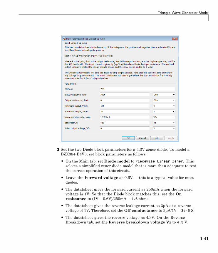
2 Set the two Band-Limited Op-Amp block parameters for the LM7301 devicewith a +–20V power supply:
• The datatsheet gives the gain as 97dB, which is equivalent to10^(97/20)=7.080e4. Set the Gain, A parameter to 7e4.
• The datatsheet gives input resistance as 39Mohms. Set Inputresistance, Rin to 39e6.
• Set Output resistance, Rout to 0 ohms. The datatsheet does not quotea value for Rout, but the term is insignificant compared to the outputresistor that it drives.
• Set minimum and maximum output voltages to –20 and +20 volts,respectively.
• The datatsheet gives the maximum slew rate as 1.25V/μs. Set theMaximum slew rate, Vdot parameter to 1.25e6 V/s.
1-40
Triangle Wave Generator Model
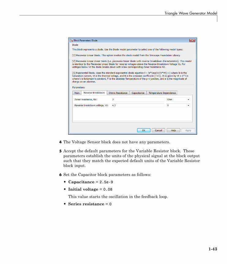
3 Set the two Diode block parameters for a 4.3V zener diode. To model aBZX384-B4V3, set block parameters as follows:
• On the Main tab, set Diode model to Piecewise Linear Zener. Thisselects a simplified zener diode model that is more than adequate to testthe correct operation of this circuit.
• Leave the Forward voltage as 0.6V — this is a typical value for mostdiodes.
• The datatsheet gives the forward current as 250mA when the forwardvoltage is 1V. So that the Diode block matches this, set the Onresistance to (1V – 0.6V)/250mA = 1.6 ohms.
• The datatsheet gives the reverse leakage current as 3μA at a reversevoltage of 1V. Therefore, set the Off conductance to 3μA/1V = 3e-6 S.
• The datatsheet gives the reverse voltage as 4.3V. On the ReverseBreakdown tab, set the Reverse breakdown voltage Vz to 4.3 V.
1-41
1 Getting Started
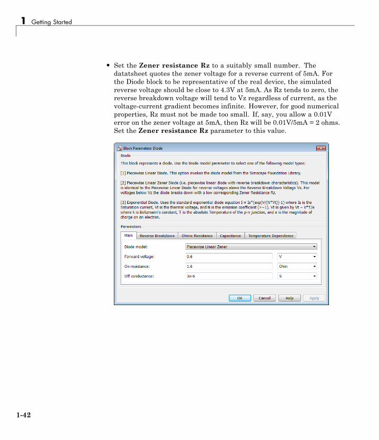
• Set the Zener resistance Rz to a suitably small number. Thedatatsheet quotes the zener voltage for a reverse current of 5mA. Forthe Diode block to be representative of the real device, the simulatedreverse voltage should be close to 4.3V at 5mA. As Rz tends to zero, thereverse breakdown voltage will tend to Vz regardless of current, as thevoltage-current gradient becomes infinite. However, for good numericalproperties, Rz must not be made too small. If, say, you allow a 0.01Verror on the zener voltage at 5mA, then Rz will be 0.01V/5mA = 2 ohms.Set the Zener resistance Rz parameter to this value.
1-42
Triangle Wave Generator Model
4 The Voltage Sensor block does not have any parameters.
5 Accept the default parameters for the Variable Resistor block. Theseparameters establish the units of the physical signal at the block outputsuch that they match the expected default units of the Variable Resistorblock input.
6 Set the Capacitor block parameters as follows:
• Capacitance = 2.5e-9
• Initial voltage = 0.08
This value starts the oscillation in the feedback loop.
• Series resistance = 0
1-43

1 Getting Started
7 Set the DC Voltage Source block parameters as follows:
• Constant voltage = 0
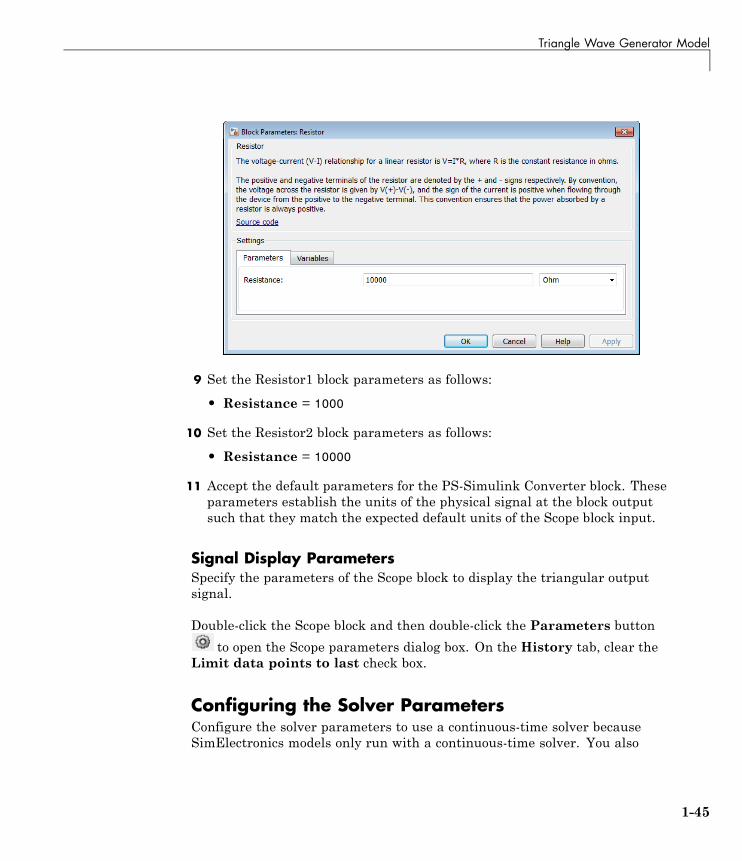
8 Set the Resistor block parameters as follows:
• Resistance = 10000
1-44
Triangle Wave Generator Model
9 Set the Resistor1 block parameters as follows:
• Resistance = 1000
10 Set the Resistor2 block parameters as follows:
• Resistance = 10000
11 Accept the default parameters for the PS-Simulink Converter block. Theseparameters establish the units of the physical signal at the block outputsuch that they match the expected default units of the Scope block input.
Signal Display ParametersSpecify the parameters of the Scope block to display the triangular outputsignal.
Double-click the Scope block and then double-click the Parameters button
to open the Scope parameters dialog box. On the History tab, clear theLimit data points to last check box.
Configuring the Solver ParametersConfigure the solver parameters to use a continuous-time solver becauseSimElectronics models only run with a continuous-time solver. You also
1-45

1 Getting Started
change the simulation end time, tighten the relative tolerance for a moreaccurate simulation, and remove the limit on the number of simulation datapoints Simulink saves.
1 In the model window, select Simulation > Model ConfigurationParameters to open the Configuration Parameters dialog box.
2 In the Solver category in the Select tree on the left side of the dialog box:
• Enter 2000e-6 for the Stop time parameter value.
• Select ode23t (Mod. stiff/Trapezoidal) from the Solver list.
• Enter 4e-5 for the Max step size parameter value.
• Enter 1e-6 for the Relative tolerance parameter value.
3 In the Data Import/Export category in the Select tree:
• Clear the Limit data points to last check box.
4 Click OK.
For more information about configuring solver parameters, see “Simulatingan Electronic System” on page 1-16.
Running the Simulation and Analyzing the ResultsRun the simulation and plot the results.
In the model window, select Simulation > Run to run the simulation.
To view the triangle wave in the Scope window, double-click the Scope block.You can do this before or after you run the simulation.
1-46
Triangle Wave Generator Model
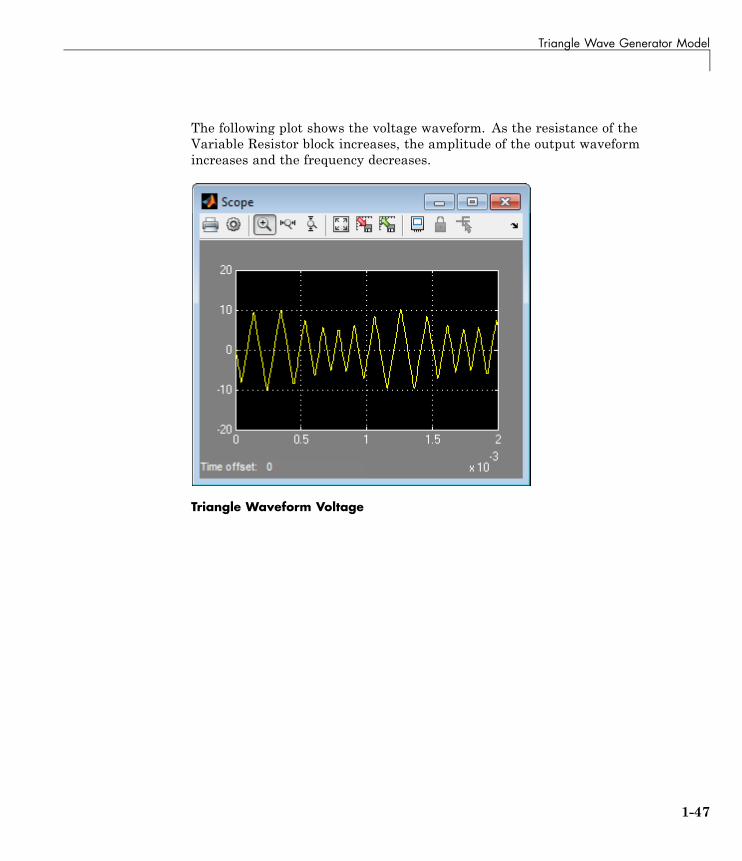
The following plot shows the voltage waveform. As the resistance of theVariable Resistor block increases, the amplitude of the output waveformincreases and the frequency decreases.
Triangle Waveform Voltage
1-47

1 Getting Started
1-48
2
Modeling an ElectronicSystem
• “Parameterizing Blocks from Datasheets” on page 2-2
• “Parameterize a Piecewise Linear Diode Model” on page 2-4
• “Parameterize an Exponential Diode from a Datasheet” on page 2-7
• “Parameterize an Exponential Diode from SPICE Netlist” on page 2-11
• “Parameterize an Op-Amp from a Datasheet” on page 2-15
• “Additional Parameterization Workflows” on page 2-17
• “Selecting the Output Model for Logic Blocks” on page 2-18
• “Simulating Thermal Effects in Semiconductors” on page 2-22
• “Simulating Thermal Effects in Rotational and Translational Actuators”on page 2-28

2 Modeling an Electronic System
Parameterizing Blocks from DatasheetsSimElectronics software is a system-level simulation tool, which providesblocks with a commensurate level of fidelity. Block parameters are designed,where possible, to match the data found on manufacturer datasheets. Forexample, the bipolar transistor blocks support parameterization in terms ofthe small-signal quantities usually quoted on a datasheet, and the underlyingmodel is simpler than that typically used by specialist EDA simulation tools.The smaller number of parameters and simpler underlying models can supportMATLAB system performance analysis better, and thereby support designchoices. Following system design, you can perform validation in hardware ormore detailed modeling and validation using an EDA simulation tool.
The following parameterization examples illustrate various blockparameterization techniques:
• Example 1: “Parameterize a Piecewise Linear Diode Model” on page 2-4
• Example 2: “Parameterize an Exponential Diode from a Datasheet” onpage 2-7
• Example 3: “Parameterize an Exponential Diode from SPICE Netlist” onpage 2-11
• Example 4: “Parameterize an Op-Amp from a Datasheet” on page 2-15
Most of the time, datasheets should be a sufficient source of parametersfor SimElectronics blocks (see Examples 1, 2, and 4). Sometimes, there isneed for more information than is available on the datasheet, and datacan be augmented from a manufacturer SPICE netlist. For example,circuit performance may depend on one or two critical components, andincreased accuracy is needed either for parameter values or the underlyingmodel. SimElectronics libraries contain a SPICE-compatible sublibrary tosupport this case, and this is illustrated by Example 3. If you have manycomponents that need to be modeled to a high level of accuracy, then Simulinkcosimulation with a specialist circuit simulator may be a better option.
In mechatronic applications in particular, you may need to model input-outputbehavior of integrated circuits, such as PWM waveform generators andH-bridges. For these two examples, SimElectronics libraries containabstracted-behavior equivalent blocks that you can use. Where you need to
2-2

Parameterizing Blocks from Datasheets
model other devices, possible options include creating your own abstractedmodel using the Simscape language, or using Simulink blocks. For an exampleof using Simulink blocks, see the Modeling an Integrated Circuit example.
When looking for a datasheet, make sure you have the originatingmanufacturer datasheet because some resellers abbreviate them.
For additional ways to parameterize and validate your model, see “AdditionalParameterization Workflows” on page 2-17.
2-3

2 Modeling an Electronic System
Parameterize a Piecewise Linear Diode ModelThe Triangle Wave Generator example model, also described in “TriangleWave Generator Model” on page 1-33, contains two zener diodes that regulatethe maximum output voltage from an op-amp amplifier circuit. Each of thesediodes is implemented with the SimElectronics Diode block, parameterizedusing the Piecewise Linear Zener option. This simple model is sufficientto check correct operation of the circuit, and requires fewer parameters thanthe Exponential option of the Diode block. However, when specifying theparameters, you need to take into account the bias condition that will be usedin the circuit. This example explains how to do this.
The Phillips Semiconductors datasheet for a BZX384–B4V3 gives thefollowing data:
Working voltage, VZ(V) at IZtest = 5mA
4.3
Diode capacitance, Cd(pF) 450
Reverse current, IR(μA) at VR = 1 V 3
Forward voltage, VF(V) at IF = 5 mA 0.7
In the datasheet, the tabulated values for VF are for higher forward currents.This value of 0.7V at 5mA is extracted from the datasheet current-voltagecurve, and is chosen as it matches the zener current used when quoting theworking voltage of 4.3V.
To match the datasheet values, the example sets the piecewise linear zenerdiode block parameters as follows:
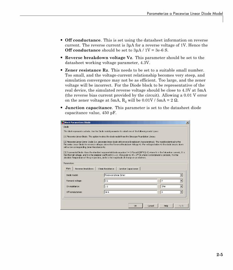
• Forward voltage. Leave as default value of 0.6V. This is a typicalvalue for most diodes, and the exact value is not critical. However, it isimportant that the value set is taken into account when calculating theOn resistance parameter.
• On resistance. This is set using the datasheet information that theforward voltage is 0.7V when the current is 5mA. The voltage to be droppedby the On resistance parameter is 0.7V minus the Forward voltageparameter, that is 0.1V. Hence the On resistance is 0.1V / 5mA = 20 Ω.
2-4
Parameterize a Piecewise Linear Diode Model
• Off conductance. This is set using the datasheet information on reversecurrent. The reverse current is 3μA for a reverse voltage of 1V. Hence theOff conductance should be set to 3μA / 1V = 3e-6 S.
• Reverse breakdown voltage Vz. This parameter should be set to thedatasheet working voltage parameter, 4.3V.
• Zener resistance Rz. This needs to be set to a suitable small number.Too small, and the voltage-current relationship becomes very steep, andsimulation convergence may not be as efficient. Too large, and the zenervoltage will be incorrect. For the Diode block to be representative of thereal device, the simulated reverse voltage should be close to 4.3V at 5mA(the reverse bias current provided by the circuit). Allowing a 0.01 V erroron the zener voltage at 5mA, RZ will be 0.01V / 5mA = 2 Ω.
• Junction capacitance. This parameter is set to the datasheet diodecapacitance value, 450 pF.
2-5

2 Modeling an Electronic System
2-6
Parameterize an Exponential Diode from a Datasheet
Parameterize an Exponential Diode from a DatasheetExample 1 uses a piecewise linear approximation to the diode’s exponentialcurrent-voltage relationship. This results in more efficient simulation, butrequires some thought to go into the setting of block parameter values.An alternative is to use a more complex model that is valid for a widerrange of voltage and current values. This example uses the Exponentialparameterization option of the Diode block.
This model either requires two data points from the diode current-voltagerelationship, or values for the underlying equation coefficients, namely thesaturation current IS and the emission coefficient N. The BZX384-B4V3datasheet only provides values for the former case. Some datasheets do notgive the necessary data for either case, and you must follow the processesin Example 1 or Example 3 instead.
The two data points in the table below are from the BZX384-B4V3 datasheetcurrent-voltage curve:
Diode forward voltage,VF
0.7V 1V
Diode forward current,IF
5mA 250mA
Set the exponential diode block parameters as follows:
• Currents [I1 I2]. Set to [5 250] mA.
• Voltages [V1 V2]. Set to [0.7 1.0] V.
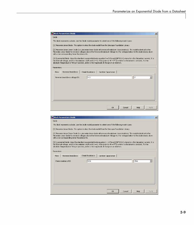
• Reverse breakdown voltage BV. Set to the datasheet working voltagevalue, 4.3V.
• Ohmic resistance. Leave at its default value of 0.01 Ω. This is anexample of a parameter that cannot be determined from the datasheet.However, setting its value to zero is not necessarily a good idea, because asmall value can help simulation convergence for some circuit topologies.The default value has negligible effect at the working current of 5mA, theadditional voltage drop being 5e-3 times 0.01 = 5e-5V. Physically, this termwill not be zero because of the connection resistances.
2-7

2 Modeling an Electronic System
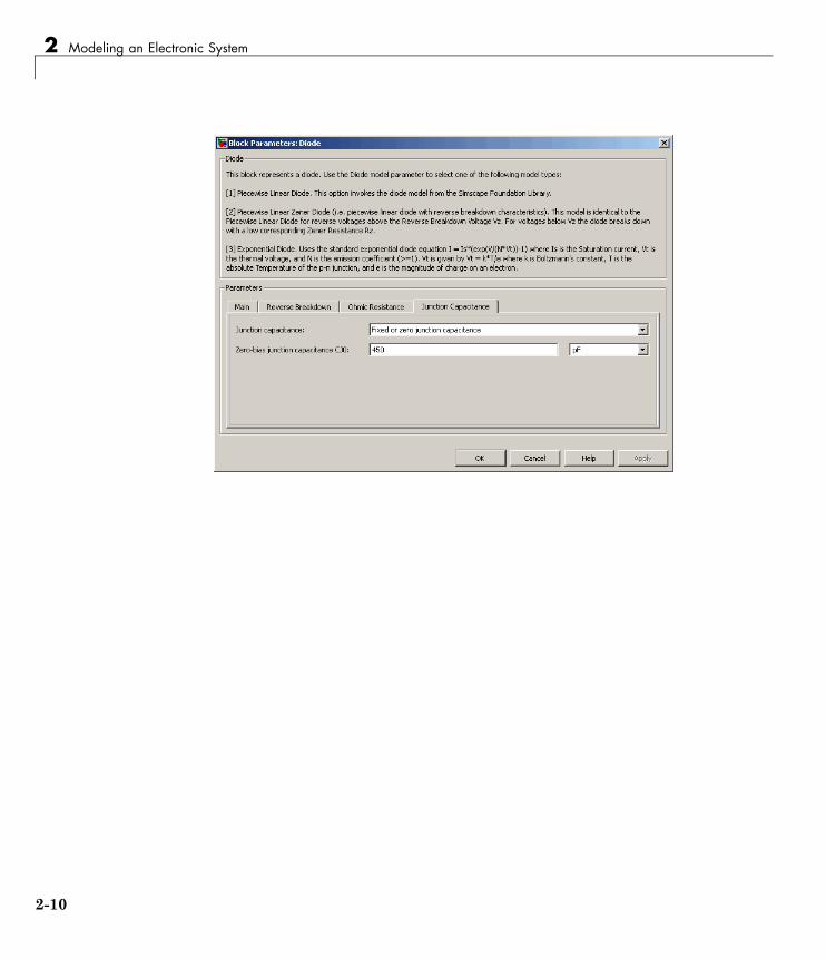
• Zero-bias junction capacitance CJ0. Set to the datasheet diodecapacitance value, 450 pF.
A more complex capacitance model is also available for the Diodecomponent with the exponential equation option. However, the datasheetdoes not provide the necessary data. Moreover, the operation of this circuitis not sufficiently sensitive to voltage-dependent capacitance effects towarrant the extra detail.
2-8
Parameterize an Exponential Diode from a Datasheet
2-9
2 Modeling an Electronic System
2-10
Parameterize an Exponential Diode from SPICE Netlist
Parameterize an Exponential Diode from SPICE NetlistIf a datasheet does not provide all of the data required by the componentmodel, another source is a SPICE netlist for the component. Componentsare defined by a particular type of SPICE netlist called a subcircuit.The subcircuit defines the coefficients for the defining equations. Mostcomponent manufacturers make subcircuits available on their websites.The format is ASCII, and you can directly read off the parameters. TheBZX384-B4V3 subcircuit can be obtained from Philips Semiconductorshttp://www.nxp.com/models/index.html.
The subcircuit data can be used to parameterize the SimElectronics Diodeblock either in conjunction with the datasheet, or on its own. For example, theOhmic resistance is defined in the subcircuit as RS = 0.387, thus providingthe missing piece of information in Example 2.
An alternative workflow is to use the SimElectronics AdditionalComponents/SPICE-Compatible Components sublibrary. The SPICE Diodeblock in this sublibrary can be directly parameterized from the subcircuit bysetting:
• Saturation current, IS to 1.033e-15
• Ohmic resistance, RS to 0.387
• Emission coefficient, ND to 1.001
• Zero-bias junction capacitance, CJO to 2.715e-10
• Junction potential, VJ to 0.7721
• Grading coefficient, MG to 0.3557
• Capacitance coefficient, FC to 0.5
• Reverse breakdown current, IBV to 0.005
• Reverse breakdown voltage, BV to 4.3
Note that where there is a one-to-one correspondence between subcircuitparameters and datasheet values, the numbers often differ. One reasonfor this is that datasheet values are sometimes given for maximum values,whereas subcircuit values are normally for nominal values. In this example,
2-11

2 Modeling an Electronic System
the CJO value of 271.5 pF differs from the datasheet capacitance of 450 pFat zero bias for this reason.
2-12

Parameterize an Exponential Diode from SPICE Netlist
2-13

2 Modeling an Electronic System
2-14
Parameterize an Op-Amp from a Datasheet
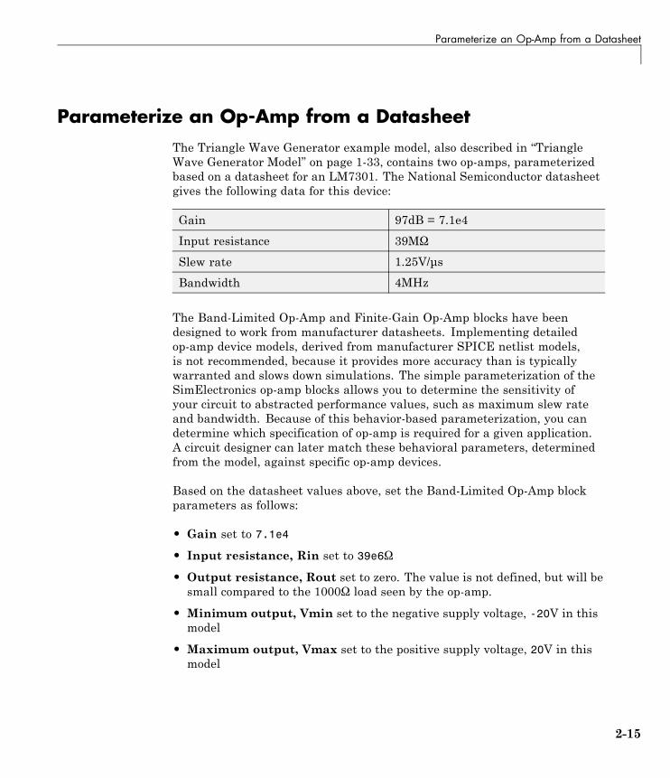
Parameterize an Op-Amp from a DatasheetThe Triangle Wave Generator example model, also described in “TriangleWave Generator Model” on page 1-33, contains two op-amps, parameterizedbased on a datasheet for an LM7301. The National Semiconductor datasheetgives the following data for this device:
Gain 97dB = 7.1e4
Input resistance 39MΩ
Slew rate 1.25V/μs
Bandwidth 4MHz
The Band-Limited Op-Amp and Finite-Gain Op-Amp blocks have beendesigned to work from manufacturer datasheets. Implementing detailedop-amp device models, derived from manufacturer SPICE netlist models,is not recommended, because it provides more accuracy than is typicallywarranted and slows down simulations. The simple parameterization of theSimElectronics op-amp blocks allows you to determine the sensitivity ofyour circuit to abstracted performance values, such as maximum slew rateand bandwidth. Because of this behavior-based parameterization, you candetermine which specification of op-amp is required for a given application.A circuit designer can later match these behavioral parameters, determinedfrom the model, against specific op-amp devices.
Based on the datasheet values above, set the Band-Limited Op-Amp blockparameters as follows:
• Gain set to 7.1e4
• Input resistance, Rin set to 39e6Ω
• Output resistance, Rout set to zero. The value is not defined, but will besmall compared to the 1000Ω load seen by the op-amp.
• Minimum output, Vmin set to the negative supply voltage, -20V in thismodel
• Maximum output, Vmax set to the positive supply voltage, 20V in thismodel
2-15

2 Modeling an Electronic System
• Maximum slew rate, Vdot set to 1.25/1e-6 V/s
• Bandwidth, f set to 4e6 Hz
Note that these parameters correspond to the values for +-5 volt operation.The datasheet also gives values for +-2.2V and +-30V operation. It is usuallybetter to pick values for a supply voltage below what your circuit uses, becauseperformance is worse at lower voltages; for example, the gain is less, and theinput impedance is less. You can use the variation in op-amp parameters withsupply voltage to suggest a typical range of parameter values for which youshould check the operation of your circuit.
2-16

Additional Parameterization Workflows
Additional Parameterization WorkflowsThere are several other ways to parameterize and validate your model:
In this section...
“Validation Using Data from SPICE Tool” on page 2-17
“Parameter Tuning Against External Data” on page 2-17
“Building an Equivalent Model of a SPICE Netlist” on page 2-17
Validation Using Data from SPICE ToolOne way to validate a parameterized SimElectronics component is to compareits behavior to data from specialist circuit simulation tool that uses amanufacturer SPICE netlist of the device. If doing this, it is important tocreate a test harness for the component that exercises it over the relevantoperating points and frequencies
Parameter Tuning Against External DataIf you have lab measurements of the device, or data from another simulationenvironment, you can use this to tune the parameters of the equivalentSimElectronics component. For an example of parameter tuning, see theexample Solar Cell Parameter Extraction From Data.
Building an Equivalent Model of a SPICE NetlistIn Example 3, parameterization from a SPICE netlist is relativelystraightforward because the netlist defines a single device (the diode) pluscorresponding model card (the parameters). Conversely, a netlist for anop-amp may have more than ten devices, plus supporting model cards. Inprinciple it is possible to build your own equivalent model of a more complexdevice by making use of the SPICE-Compatible Components sublibrary,and connecting them together using the information in the netlist. Beforeembarking on this you should ensure that the SPICE-Compatible Componentssublibrary has all of the component models that you need.
If the device models you wish to model are complex (hundreds of components),then cosimulation with an external circuit simulator may be a better approach.
2-17

2 Modeling an Electronic System
Selecting the Output Model for Logic Blocks
In this section...
“Available Output Models” on page 2-18
“Quadratic Model Output and Parameters” on page 2-19
Available Output ModelsThe blocks in the Logic sublibrary of the Integrated Circuits library provide achoice of two output models:
• Linear — Models the gate output as a voltage source driving a seriesresistor and capacitor connected to ground. This is suitable for logiccircuit operation under normal conditions and when the logic gate drivesother high-impedance CMOS gates. The block sets the value of the gateoutput capacitor such that the resistor-capacitor time constant equals thePropagation delay parameter value. The linear output model is shownin the following illustration.
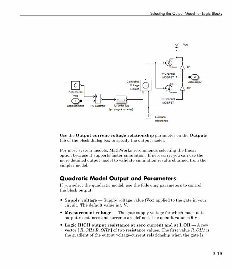
• Quadratic — Models the gate output in terms of a complementaryN-channel and P-channel MOSFET pair. This adds more fidelity, whichbecomes relevant if drawing higher currents from the gate output, or ifexercising the gate under fault conditions. In addition, the gate inputdemand is lagged to approximate the Propagation delay parametervalue. Default parameters are representative of the 74HC logic gate family.The quadratic output model is shown in the next illustration.
2-18
Selecting the Output Model for Logic Blocks
Use the Output current-voltage relationship parameter on the Outputstab of the block dialog box to specify the output model.
For most system models, MathWorks recommends selecting the linearoption because it supports faster simulation. If necessary, you can use themore detailed output model to validate simulation results obtained from thesimpler model.
Quadratic Model Output and ParametersIf you select the quadratic model, use the following parameters to controlthe block output:
• Supply voltage— Supply voltage value (Vcc) applied to the gate in yourcircuit. The default value is 5 V.
• Measurement voltage — The gate supply voltage for which mask dataoutput resistances and currents are defined. The default value is 5 V.
• Logic HIGH output resistance at zero current and at I_OH— A rowvector [ R_OH1 R_OH2 ] of two resistance values. The first value R_OH1 isthe gradient of the output voltage-current relationship when the gate is
2-19
2 Modeling an Electronic System
logic HIGH and there is no output current. The second value R_OH2 is thegradient of the output voltage-current relationship when the gate is logicHIGH and the output current is I_OH. The default value is [ 25 250 ] Ω.
• Logic HIGH output current I_OH when shorted to ground — Theresulting current when the gate is in the logic HIGH state, but the loadforces the output voltage to zero. The default value is 63 mA.
• Logic LOW output resistance at zero current and at I_OL — A rowvector [ R_OL1 R_OL2 ] of two resistance values. The first value R_OL1 isthe gradient of the output voltage-current relationship when the gate islogic LOW and there is no output current. The second value R_OL2 is thegradient of the output voltage-current relationship when the gate is logicLOW and the output current is I_OL. The default value is [ 30 800 ] Ω.
• Logic LOW output current I_OL when shorted to Vcc— The resultingcurrent when the gate is in the logic LOW state, but the load forces theoutput voltage to the supply voltage Vcc. The default value is -45 mA.
• Propagation delay — Time it takes for the output to swing from LOWto HIGH or HIGH to LOW after the input logic levels change. For quadraticoutput, it is implemented by the lagged gate input demand. The defaultvalue is 25 ns.
• Protection diode on resistance — The gradient of the voltage-currentrelationship for the protection diodes when forward biased. The defaultvalue is 5 Ω.
• Protection diode forward voltage — The voltage above which theprotection diode is turned on. The default value is 0.6 V.
The following graphic illustrates the quadratic output model parameterization,using the default parameter output characteristics for a +5V supply.
2-20

Selecting the Output Model for Logic Blocks
2-21
2 Modeling an Electronic System
Simulating Thermal Effects in Semiconductors
In this section...
“Using the Thermal Ports” on page 2-22
“Thermal Model for Semiconductor Blocks” on page 2-24
“Thermal Mass Parameterization” on page 2-25
“Electrical Behavior Depending on Temperature” on page 2-26
“Improving Numerical Performance” on page 2-26
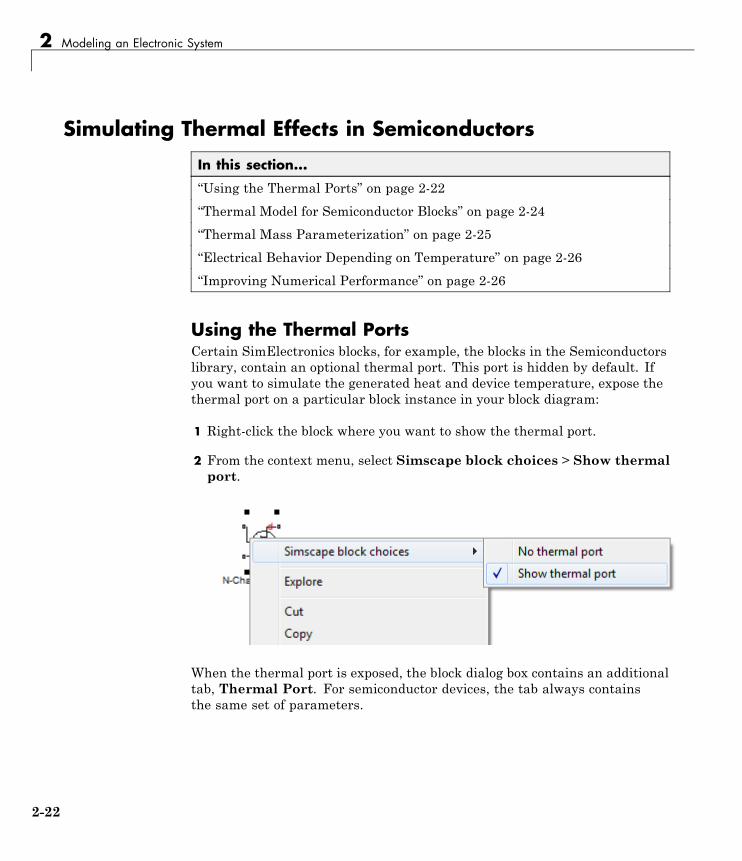
Using the Thermal PortsCertain SimElectronics blocks, for example, the blocks in the Semiconductorslibrary, contain an optional thermal port. This port is hidden by default. Ifyou want to simulate the generated heat and device temperature, expose thethermal port on a particular block instance in your block diagram:
1 Right-click the block where you want to show the thermal port.
2 From the context menu, select Simscape block choices > Show thermalport.
When the thermal port is exposed, the block dialog box contains an additionaltab, Thermal Port. For semiconductor devices, the tab always containsthe same set of parameters.
2-22

Simulating Thermal Effects in Semiconductors
• Junction case and case-ambient (or case-heatsink) thermalresistances, [R_JC R_CA]— A row vector [ R_JC R_CA ] of two thermalresistance values, represented by the two Conductive Heat Transfer blocksin the “Thermal Model for Semiconductor Blocks” on page 2-24. The firstvalue R_JC is the thermal resistance between the junction and case. Thesecond value R_CA is the thermal resistance between port H and the devicecase. See “Thermal Model for Semiconductor Blocks” on page 2-24 forfurther details. The default value is [ 0 10 ]K/W.
• Thermal mass parameterization — Select whether you want toparameterize the thermal masses in terms of thermal time constants(By thermal time constants), or specify the thermal mass valuesdirectly (By thermal mass). For more information, see “Thermal MassParameterization” on page 2-25. The default is By thermal timeconstants.
• Junction and case thermal time constants, [t_J t_C] — A rowvector [ t_J t_C ] of two thermal time constant values. The first valuet_J is the junction time constant. The second value t_C is the case timeconstant. This parameter is only visible when you select By thermal timeconstants for the Thermal mass parameterization parameter. Thedefault value is [ 0 10 ] s.
• Junction and case thermal masses, [M_J M_C] — A row vector[ M_J M_C ] of two thermal mass values. The first value M_J is thejunction thermal mass. The second value M_C is the case thermal mass.This parameter is only visible when you select By thermal mass for theThermal mass parameterization parameter. The default value is [ 01 ] J/K.
2-23

2 Modeling an Electronic System
• Junction and case initial temperatures, [T_J T_C] — A row vector [T_J T_C ] of two temperature values. The first value T_J is the junctioninitial temperature. The second value T_C is the case initial temperature.The default value is [ 25 25 ] C.
For more information on selecting the parameter values, see “ThermalModel for Semiconductor Blocks” on page 2-24 and “Improving NumericalPerformance” on page 2-26. For explanation of the relationship between theThermal Port and Temperature Dependence tabs in a block dialog box,see “Electrical Behavior Depending on Temperature” on page 2-26.
Thermal Model for Semiconductor BlocksAll blocks with optional thermal ports include an internal thermal modelwith thermal masses and resistances. The purpose of including this modelinternally is to keep your diagram uncluttered by the thermal model. Thefollowing figure shows an equivalent model of the internal thermal model forsemiconductor devices.
The port H in the diagram corresponds to the thermal port H of the block.The two Thermal Mass blocks represent the thermal mass of the device caseand the thermal mass of the semiconductor junction, respectively. The IdealHeat Flow Source block inputs heat to the model with value equal to theelectrically generated heat from the device.
The two Conductive Heat Transfer blocks model the thermal resistances.Resistance R_JC (conductance 1/R_JC) represents the thermal resistancebetween junction and case. Because of this resistance, under normalconditions the junction will be hotter than the case. Resistance R_CArepresents the thermal resistance between port H and the device case. If thedevice has no heatsink, then in your model you should connect port H to an
2-24
Simulating Thermal Effects in Semiconductors
Ideal Temperature Source with its temperature set to ambient conditions.If your device does have an external heatsink, then you must model theheatsink externally to the device, and connect the heatsink thermal massdirectly to port H.
If you wish to keep all or part of the thermal model of the device external tothe model, you can set the necessary block parameters to zero. The followingrules apply:
• Case thermal mass must be greater than zero.
• Junction thermal mass can only be set to zero if the junction-case resistanceis also set to zero.
• If both case and junction thermal masses are defined, but junction-caseresistance is zero, then the initial temperatures assigned to junction andcase must be identical.
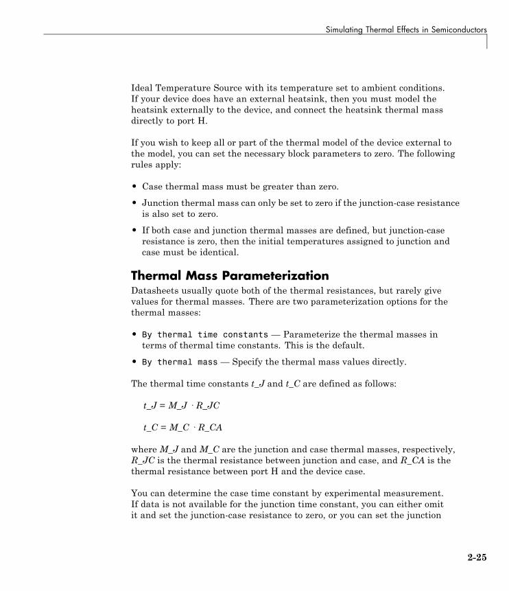
Thermal Mass ParameterizationDatasheets usually quote both of the thermal resistances, but rarely givevalues for thermal masses. There are two parameterization options for thethermal masses:
• By thermal time constants — Parameterize the thermal masses interms of thermal time constants. This is the default.
• By thermal mass— Specify the thermal mass values directly.
The thermal time constants t_J and t_C are defined as follows:
t_J = M_J · R_JC
t_C = M_C · R_CA
where M_J and M_C are the junction and case thermal masses, respectively,R_JC is the thermal resistance between junction and case, and R_CA is thethermal resistance between port H and the device case.
You can determine the case time constant by experimental measurement.If data is not available for the junction time constant, you can either omitit and set the junction-case resistance to zero, or you can set the junction
2-25

2 Modeling an Electronic System
time constant to a typical value of one tenth of the case time constant. Thealternative is to estimate thermal masses based on device dimensions andaveraged material specific heats.
Electrical Behavior Depending on TemperatureFor blocks with optional thermal ports, there are two simulation options:
• Simulate the generated heat, device temperature, and the effect oftemperature on the electrical equations.
• Simulate the generated heat and device temperature, but do not includeeffect of temperature on the electrical equations. Use this option whenthe impact of temperature on the electrical equations is small over thetemperature range to be simulated, or where the primary task of thesimulation is to capture the heat generated to support system-level design.
The thermal port and the Thermal Port tab of the block dialog box letyou simulate the generated heat and device temperature. The ThermalDependence tab of the block dialog box lets you model the effect oftemperature of the semiconductor junction on the electrical equations.Therefore:
• To simulate all the temperature effects, show the block’s thermal port andset the Parameterization parameter on the Thermal Dependence tab toModel temperature dependence (or, for blocks with a choice of options formodeling temperature dependence, select one of these options, for example,Use an I-V data point at second measurement temperature).
• To simulate just the generated heat and device temperature, showthe block’s thermal port but set the Parameterization parameter onthe Thermal Dependence tab to None Simulate at parametermeasurement temperature.
Improving Numerical PerformanceIt is very important that you set realistic values for thermal masses andresistances. Otherwise, junction temperatures can become extreme, and outof range for valid results, which in turn may manifest itself as numericaldifficulties when simulating. A simple test to see if numerical difficulties are aresult of unrealistic thermal values is to turn off the temperature dependence
2-26

Simulating Thermal Effects in Semiconductors
for the electrical equations, by setting the Parameterization parameteron the Thermal Dependence tab to None Simulate at parametermeasurement temperature.
The thermal time constants are generally much slower than electricaltime constants, so the thermal aspects of your model are unlikely todictate the maximum fixed time step you can simulate at (for example, forhardware-in-the-loop simulations). However, if you need to remove detail (forexample, to speed up simulation), the junction thermal mass time constantis typically an order of magnitude faster than the case thermal mass timeconstant. You can remove the effect of the junction thermal mass by settingthe junction thermal mass to zero and also setting the junction-case thermalresistance to zero.
2-27

2 Modeling an Electronic System
Simulating Thermal Effects in Rotational and TranslationalActuators
In this section...
“Using the Thermal Ports” on page 2-28
“Thermal Model for Actuator Blocks” on page 2-30
Using the Thermal PortsAll blocks that represent rotational and translational actuators with electricalwindings can optionally show a thermal port for each electrical winding. So,for example:
• A DC Motor block can optionally show a single thermal port correspondingto the armature
• A Shunt Motor block can optionally show two thermal ports, one for thestator winding and one for the field winding
The thermal port represents copper resistance losses which convert electricalpower to heat. These losses are sometimes referred to as i2R losses. Thethermal ports do not represent iron losses due to, for example, Eddy currentsand hysteresis.
The thermal ports are hidden by default. To expose the thermal port on aparticular block instance in your block diagram:
1 Right-click the block where you want to show the thermal port.
2 From the context menu, select Simscape block choices > Show thermalport.
2-28

Simulating Thermal Effects in Rotational and Translational Actuators
When the thermal port is exposed, the block dialog box contains two additionaltabs, Temperature Dependence and Thermal Port. For actuator blockswith single winding, these tabs always contain the same set of parameters.
• Resistance temperature coefficient — Parameter α in the equationdefining resistance as a function of temperature, as described in “ThermalModel for Actuator Blocks” on page 2-30. The default value is for copper,and is 0.00393 1/K.
• Measurement temperature — The temperature for which motorparameters are defined. The default value is 25 C.
2-29
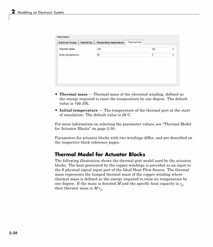
2 Modeling an Electronic System
• Thermal mass — Thermal mass of the electrical winding, defined asthe energy required to raise the temperature by one degree. The defaultvalue is 100 J/K.
• Initial temperature — The temperature of the thermal port at the startof simulation. The default value is 25 C.
For more information on selecting the parameter values, see “Thermal Modelfor Actuator Blocks” on page 2-30.
Parameters for actuator blocks with two windings differ, and are described onthe respective block reference pages.
Thermal Model for Actuator BlocksThe following illustration shows the thermal port model used by the actuatorblocks. The heat generated by the copper windings is provided as an input tothe S physical signal input port of the Ideal Heat Flow Source. The thermalmass represents the lumped thermal mass of the copper winding wherethermal mass is defined as the energy required to raise its temperature byone degree. If the mass is denoted M and the specific heat capacity is cp,then thermal mass is M·cp.
2-30
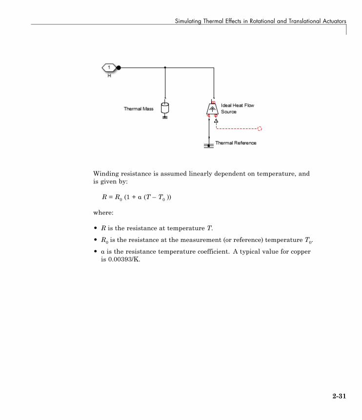
Simulating Thermal Effects in Rotational and Translational Actuators
Winding resistance is assumed linearly dependent on temperature, andis given by:
R = R0 (1 + α (T – T0 ))
where:
• R is the resistance at temperature T.
• R0 is the resistance at the measurement (or reference) temperature T0.
• α is the resistance temperature coefficient. A typical value for copperis 0.00393/K.
2-31