Simulations over South Asia using the Weather Research · PDF fileprovide information on the...
23
Geosci. Model Dev., 5, 321–343, 2012 www.geosci-model-dev.net/5/321/2012/ doi:10.5194/gmd-5-321-2012 © Author(s) 2012. CC Attribution 3.0 License. Geoscientific Model Development Simulations over South Asia using the Weather Research and Forecasting model with Chemistry (WRF-Chem): set-up and meteorological evaluation R. Kumar 1 , M. Naja 1 , G. G. Pfister 2 , M. C. Barth 2 , and G. P. Brasseur 3 1 Aryabhatta Research Institute of Observational Sciences, Nainital, 263129, India 2 Atmospheric Chemistry Division, NCAR, Boulder, CO 80307-3000, USA 3 Climate Service Center, Helmholtz Zentrum Geesthacht, Hamburg 20146, Germany Correspondence to: M. Naja ([email protected]) Received: 14 November 2011 – Published in Geosci. Model Dev. Discuss.: 22 November 2011 Revised: 8 February 2012 – Accepted: 21 February 2012 – Published: 20 March 2012 Abstract. The configuration and evaluation of the meteo- rology is presented for simulations over the South Asian re- gion using the Weather Research and Forecasting model cou- pled with Chemistry (WRF-Chem). Temperature, water va- por, dew point temperature, zonal and meridional wind com- ponents, precipitation and tropopause pressure are evaluated against radiosonde and satellite-borne (AIRS and TRMM) observations along with NCEP/NCAR reanalysis fields for the year 2008. Chemical fields, with focus on tropospheric ozone, are evaluated in a companion paper. The spatial and temporal variability in meteorological variables is well sim- ulated by the model with temperature, dew point temper- ature and precipitation showing higher values during sum- mer/monsoon and lower during winter. The index of agree- ment for all the parameters is estimated to be greater than 0.6 indicating that WRF-Chem is capable of simulating the vari- ations around the observed mean. The mean bias (MB) and root mean square error (RMSE) in modeled temperature, wa- ter vapor and wind components show an increasing tendency with altitude. MB and RMSE values are within ±2 K and 1– 4 K for temperature, 30 % and 20–65 % for water vapor and 1.6 m s -1 and 5.1 m s -1 for wind components. The spatio- temporal variability of precipitation is also reproduced rea- sonably well by the model but the model overestimates pre- cipitation in summer and underestimates precipitation dur- ing other seasons. Such a behavior of modeled precipitation is in agreement with previous studies on South Asian mon- soon. The comparison with radiosonde observations indi- cates a relatively better model performance for inland sites as compared to coastal and island sites. The MB and RMSE in tropopause pressure are estimated to be less than 25 hPa. Sensitivity simulations show that biases in meteorological simulations can introduce errors of ± (10–25 %) in simula- tions of tropospheric ozone, CO and NO x . Nevertheless, a comparison of statistical metrics with benchmarks indicates that the model simulated meteorology is of sufficient quality for use in chemistry simulations. 1 Introduction South Asia is characterized by a widely-varying landscape including the elevated Himalayan terrain, semi-arid and desert land masses, tropical rainforests, sea-shores and the vast plains. This region stretches from Afghanistan and Pak- istan in the west to the northeastern provinces of India and Myanmar in the east and is bounded to the north by China and to the south by the Indian Ocean. Apart from this natu- ral landscape diversity, the anthropogenic emissions of trace gases and aerosols are increasing rapidly over this region (e.g. Akimoto, 2003; Ohara et al., 2007). The pollutants em- anating from South Asia may have a wide range of potential consequences for the air quality, radiation budget and the at- mospheric chemistry on the regional to global scales (e.g. Ramanathan and Crutzen, 2003; Lawrence and Lelieveld, 2010). Further, South Asia is a region of intense photochem- ical activity due to the availability of strong tropical solar radiation and high humidity. In light of the above conditions, in situ measurements of different trace species, in particular of ozone and aerosols, have been initiated over the Indian region in the 1990s (e.g. Lal et al., 2000; Babu et al., 2002; Naja and Lal, 2002; Sagar et al., 2004; Jain et al., 2005; Niranjan et al., 2006; Satheesh et al., 2008). In addition, only a few national and Published by Copernicus Publications on behalf of the European Geosciences Union.
Transcript of Simulations over South Asia using the Weather Research · PDF fileprovide information on the...
Geosci. Model Dev., 5, 321–343, 2012www.geosci-model-dev.net/5/321/2012/doi:10.5194/gmd-5-321-2012© Author(s) 2012. CC Attribution 3.0 License.
GeoscientificModel Development
Simulations over South Asia using the Weather Research andForecasting model with Chemistry (WRF-Chem): set-up andmeteorological evaluation
R. Kumar 1, M. Naja1, G. G. Pfister2, M. C. Barth 2, and G. P. Brasseur3
1Aryabhatta Research Institute of Observational Sciences, Nainital, 263129, India2Atmospheric Chemistry Division, NCAR, Boulder, CO 80307-3000, USA3Climate Service Center, Helmholtz Zentrum Geesthacht, Hamburg 20146, Germany
Correspondence to:M. Naja ([email protected])
Received: 14 November 2011 – Published in Geosci. Model Dev. Discuss.: 22 November 2011Revised: 8 February 2012 – Accepted: 21 February 2012 – Published: 20 March 2012
Abstract. The configuration and evaluation of the meteo-rology is presented for simulations over the South Asian re-gion using the Weather Research and Forecasting model cou-pled with Chemistry (WRF-Chem). Temperature, water va-por, dew point temperature, zonal and meridional wind com-ponents, precipitation and tropopause pressure are evaluatedagainst radiosonde and satellite-borne (AIRS and TRMM)observations along with NCEP/NCAR reanalysis fields forthe year 2008. Chemical fields, with focus on troposphericozone, are evaluated in a companion paper. The spatial andtemporal variability in meteorological variables is well sim-ulated by the model with temperature, dew point temper-ature and precipitation showing higher values during sum-mer/monsoon and lower during winter. The index of agree-ment for all the parameters is estimated to be greater than 0.6indicating that WRF-Chem is capable of simulating the vari-ations around the observed mean. The mean bias (MB) androot mean square error (RMSE) in modeled temperature, wa-ter vapor and wind components show an increasing tendencywith altitude. MB and RMSE values are within±2 K and 1–4 K for temperature, 30 % and 20–65 % for water vapor and1.6 m s−1 and 5.1 m s−1 for wind components. The spatio-temporal variability of precipitation is also reproduced rea-sonably well by the model but the model overestimates pre-cipitation in summer and underestimates precipitation dur-ing other seasons. Such a behavior of modeled precipitationis in agreement with previous studies on South Asian mon-soon. The comparison with radiosonde observations indi-cates a relatively better model performance for inland sitesas compared to coastal and island sites. The MB and RMSEin tropopause pressure are estimated to be less than 25 hPa.Sensitivity simulations show that biases in meteorological
simulations can introduce errors of± (10–25 %) in simula-tions of tropospheric ozone, CO and NOx. Nevertheless, acomparison of statistical metrics with benchmarks indicatesthat the model simulated meteorology is of sufficient qualityfor use in chemistry simulations.
1 Introduction
South Asia is characterized by a widely-varying landscapeincluding the elevated Himalayan terrain, semi-arid anddesert land masses, tropical rainforests, sea-shores and thevast plains. This region stretches from Afghanistan and Pak-istan in the west to the northeastern provinces of India andMyanmar in the east and is bounded to the north by Chinaand to the south by the Indian Ocean. Apart from this natu-ral landscape diversity, the anthropogenic emissions of tracegases and aerosols are increasing rapidly over this region(e.g. Akimoto, 2003; Ohara et al., 2007). The pollutants em-anating from South Asia may have a wide range of potentialconsequences for the air quality, radiation budget and the at-mospheric chemistry on the regional to global scales (e.g.Ramanathan and Crutzen, 2003; Lawrence and Lelieveld,2010). Further, South Asia is a region of intense photochem-ical activity due to the availability of strong tropical solarradiation and high humidity.
In light of the above conditions, in situ measurements ofdifferent trace species, in particular of ozone and aerosols,have been initiated over the Indian region in the 1990s (e.g.Lal et al., 2000; Babu et al., 2002; Naja and Lal, 2002;Sagar et al., 2004; Jain et al., 2005; Niranjan et al., 2006;Satheesh et al., 2008). In addition, only a few national and
Published by Copernicus Publications on behalf of the European Geosciences Union.

322 R. Kumar et al.: WRF-Chem over South Asia: meteorological evaluation
international campaigns such as the Indian Ocean Experi-ment (INDOEX) (Ramanathan et al., 2001; Lelieveld et al.,2001) and the Integrated Campaign for Aerosols, gases andRadiation Budget (ICARB) (Moorthy et al., 2008) have beenconducted over the adjoining marine regions of the ArabianSea, Bay of Bengal and Indian Ocean to study the impactof South Asian emissions on the pristine oceanic environ-ments and export of pollutants from this region. Further, ayearlong intensive field campaign (Regional Aerosol Warm-ing Experiment (RAWEX) – Ganges Valley Aerosol Experi-ment (GVAX) is being carried out over Northern India withARIES, Nainital as a main site to study the impact of aerosolson cloud formation and precipitation (http://www.arm.gov/sites/amf/pgh). Although these measurements provide highlyvaluable information about the diurnal and seasonal variabil-ity of trace species they are not sufficient to derive informa-tion on the regional distribution of trace gases and aerosols.Due to the scarcity of in situ observations, the additional useof chemical transport models is essential for understandingthe spatio-temporal distribution of trace species in this regionand their implications on the air quality and climate.
Previous studies have focused on simulating the distri-bution of ozone and related species over this region usingregional (e.g. Roy et al., 2008; Engardt, 2008) and globalchemical transport models (e.g. Beig and Brasseur, 2006).However, all these studies used offline models which gener-ally decouple the chemical and meteorological processes byusing the output of a standard meteorological model as theinput for the chemical model and thus have some inevitablelimitations. For instance, these models do not allow feed-backs between the chemistry and meteorology and may missimportant information about the short-term atmospheric pro-cesses. In this study we employ a fully coupled online re-gional air quality model known as the “Weather Research andForecasting model coupled with Chemistry” (WRF-Chem)(Grell et al., 2005). The meteorological and chemical com-ponents of the chemistry modules use the same horizontaland vertical coordinates and the same physical parameteriza-tion as the meteorological model. The model does not per-form any time interpolation and allows the feedback betweenchemical and meteorological processes (Grell et al., 2005).
Several studies have validated the WRF-Chem modelagainst observations over North America (e.g. McKeen etal., 2005; Tie et al., 2007), Europe (Schurmann et al., 2009)and East Asia (Matsui et al., 2009). However, such effortshave not been made so far over the South Asian region. TheWRF model has been employed earlier over the Indian re-gion to study extreme weather events (e.g. Rajeevan et al.,2010; Dutta and Prasad, 2010), the monsoon depressions(e.g. Chang et al., 2009) and to study impact of assimilationschemes on short range forecasts (e.g. Rakesh et al., 2009).These studies indicate that the WRF model has good abil-ity to simulate these events and produces much better fore-casts with assimilated fields. However, these studies did notprovide information on the skill of WRF in simulating the
year-long meteorology of this region. Therefore, this studyis aimed at evaluation and quantification of errors and bi-ases in WRF-Chem simulated meteorological fields over thecourse of all seasons and impact of meteorological errorson chemistry simulations with focus on tropospheric ozone.Such evaluation is essential to establish the model’s credibil-ity for future studies. In this manuscript, the meteorologi-cal fields simulated by the WRF-Chem model are evaluatedagainst a set of balloon-borne and space-borne observationsand reanalysis datasets. The evaluation of chemical fields isdiscussed in another manuscript (Kumar et al., 2012).
Ground-based observations are amongst the most accurateand reliable dataset for evaluating the model performance inregard to air quality but these measurements have limited ge-ographical and altitude coverage over the Indian region andare highly sparse over the remote oceanic and mountainousregions. This spatial heterogeneity in the availability of insitu observations might lead to a sampling bias in the modelevaluation. The gap in spatial heterogeneity can be mini-mized to a large extent by the use of satellite observations andreanalysis datasets. The satellites provide daily global threedimensional observations of the atmospheric state while thereanalysis datasets are generated by the quality controlled as-similation of observations from different platforms such asfrom land, ship, aircraft, radiosonde and pibal (pilot balloon)etc.
In this study, we used temperature and dew point tem-perature from radiosonde observations, temperature, watervapor and tropopause pressure retrieved by the atmosphericinfrared sounder (AIRS), daily total precipitation amountsfrom the Tropical Rainfall Measuring Mission (TRMM), aswell as NCEP/NCAR reanalysis zonal and meridional windcomponents for the evaluation of WRF-Chem meteorologi-cal fields. The outline of the manuscript is as follows. Wefirst give a description of the WRF-Chem model configura-tion in Sect. 2. The information on different observationaldatasets, the reanalysis fields and the evaluation methodol-ogy used in this study are presented in Sect. 3. The evalu-ation and sensitivity results are described in Sect. 4 and aresummarized in Sect. 5.
2 The model description
This study uses version 3.1.1 of the fully compressibleand non-hydrostatic Advanced Research WRF model (http://www.mmm.ucar.edu/wrf/users/) coupled with Chemistry(WRF-Chem;http://ruc.fsl.noaa.gov/wrf/WG11) developedjointly by NOAA, DOE/PNNL, NCAR and other researchinstitutes. The WRF model (Skamarock et al., 2008) usesthe terrain-following hydrostatic pressure as the vertical co-ordinate and Arakawa-C grid for grid staggering. The modeluses the Runge-Kutta second and third order time integrationschemes and second to sixth order advection schemes in boththe horizontal and vertical directions. A time-split small step
Geosci. Model Dev., 5, 321–343, 2012 www.geosci-model-dev.net/5/321/2012/

R. Kumar et al.: WRF-Chem over South Asia: meteorological evaluation 323
60E 70E 80E 90E 100E
10N
20N
30N
40N
0250500750100012501500175020002250250027503000325035003750400042504500475050005250550057506000
Surface Elevation (m)
Fig. 1. The simulation domain and the topography used by the model. The geographic locations of RAOB sites used in this study are alsoshown. The description of station codes is provided in Table 1.
scheme is used for an acoustic and gravity-wave model. Inthis study, the simulation domain is defined on the Merca-tor projection centered at 25◦ N, 80◦ E (Fig. 1). The domaincovers nearly the entire South Asian region with a 45 km spa-tial resolution and has 90 grid points in both the west-eastand the north-south directions. The 45 km resolution is cho-sen because the fine-scale anthropogenic emissions data areavailable at 0.5◦ resolution, which limits the model resolu-tion. There are 51 vertical levels in the model from the sur-face to∼30 km (10 hPa), 10 of which are located within 1 kmabove the model surface. The model top is placed at 10 hPabecause modeled vertical ozone distribution showed betteragreement with observations with higher (10 hPa) model topas compared to lower (50 hPa) model top.
The static geographical fields such as the terrain height,land-use/vegetation, soil properties, vegetation fraction andalbedo etc. are interpolated from 10 min (approximately19 km) United States Geological Survey (USGS) data to thesimulation domain by using the geogrid program of the WRFpreprocessing system (WPS). The surface terrain (Fig. 1)used by the model has an important influence on the me-teorology and chemical distributions. The northern part ofSouth Asia with the Himalaya Mountains has a montane andtemperate climate, while the southern part is surrounded byoceans and experiences a mostly moist climate. The dri-est weather prevails in the Great Indian Thar Desert (∼24◦–30◦ N; ∼70◦–75◦ E) in western India. Forested regions aregenerally found at high altitude and high rainfall regions innorthern, north-eastern and southern parts of India. Further
details regarding the topographical features, land-use andclassification patterns in India can be found on the websiteof the Ministry of Environment and Forests, Government ofIndia (http://moef.nic.in/index.php). The initial and lateralboundary conditions for meteorological parameters are ob-tained from NCEP Final analysis (FNL) fields available ev-ery 6 h at the spatial resolution of 1◦
× 1◦.
The resolved-scale cloud physics is represented by theThompson microphysics scheme (Thompson et al., 2004),which includes seven moisture variables undergoing liquid-phase, ice-phase and mixed-phase processes. The sub-gridscale effects of convective and shallow clouds are param-eterized according to the Kain-Fritsch convective scheme(Kain, 2004). The Rapid Radiative Transfer Model (RRTM)long-wave radiation scheme (Mlawer et al., 1997) is used torepresent long-wave radiative processes due to water vapor,clouds and trace gases (e.g. CO2, ozone etc.). The short-wave radiative processes are incorporated using the Goddardshort-wave scheme (Chou and Suarez, 1994). The feed-back from the aerosols to the radiation scheme has beenturned on in the simulation. The aerosol module used hereis based on the Modal Aerosol Dynamics Model for Eu-rope/Secondary Organic Aerosol Model (MADE/SORGAM)(Ackermann et al., 1998; Schell et al., 2001) and dust emis-sions are calculated online within the model using land-scape and meteorological information. The friction veloci-ties and exchange coefficients that enable the calculation ofsurface thermal and moisture fluxes by land-surface modeland surface stress in the planetary boundary layer scheme
www.geosci-model-dev.net/5/321/2012/ Geosci. Model Dev., 5, 321–343, 2012
324 R. Kumar et al.: WRF-Chem over South Asia: meteorological evaluation
Table 1. Details and the categorization of the RAOB sites used in this study.
Station Station Longitude Latitude Actual Model CategoryName Code (◦ E) (◦ N) Altitude∗ Altitude∗
Bhubaneswar BHU 85.83 20.25 46 47
Coastal Sites
Bombay BOM 72.85 19.12 14 42Machilipatnam MAC 81.15 16.20 3 3Goa/Panjim GOA 73.82 15.48 60 120Madras MAD 80.18 13.00 16 22Panambur PAN 74.83 12.95 31 45Vishakhapatnam VIS 83.30 17.70 66 54Thiruvanantpuram THI 76.95 8.48 64 100Karaikal KAR 79.83 10.92 7 3Cochin COC 76.27 9.95 3 15
Port-Blair POR 92.72 11.67 79 8Island SitesMinicoy-Island MIN 73.15 8.30 2 0
Amini-Divi AMI 72.73 11.12 4 0
Patiala PAT 76.47 30.33 251 245
Low Altitude Sites
Delhi DEL 77.20 28.58 216 213Dibrugarh DIB 95.02 27.48 111 57Jodhpur JOD 73.02 26.30 224 225Gwalior GWA 78.25 26.23 207 191Lucknow LUC 80.88 26.75 128 123Gorakhpur GOR 83.37 26.75 77 64Siliguri SIL 88.37 26.67 123 224Gauhati GAU 91.58 26.10 54 298Patna PAT 85.10 25.60 60 45Ahmedabad AHM 72.63 23.07 55 54Raipur RAI 81.67 21.22 298 283Nagpur NAG 79.05 21.10 310 322Agartala AGA 91.25 23.88 16 25Calcutta CAL 88.45 22.65 6 6
Aurangabad AUR 75.40 19.85 579 559
Moderately High
Bhopal BHO 77.35 23.28 523 467
Altitude Sites
Ranchi RAN 85.32 23.32 652 502Jagdalpur JAG 82.03 19.08 553 564Hyderabad HYD 78.47 17.45 545 537Bangalore BAN 77.58 12.97 921 853
∗ The altitude values are in meters above mean sea level (a.m.s.l.).
are calculated according to Monin-Obukhov similarity the-ory using the Eta surface layer scheme (Janjic, 1996). Theunified Noah land-surface model (Chen and Dudhia, 2001),using USGS 1 km land-surface data is used to obtain thermaland moisture fluxes from the surface. The vertical sub-gridscale fluxes due to eddy transports in the planetary boundarylayer and the free atmosphere are parameterized accordingto the Mellor-Yamada-Janjic (MYJ) boundary layer scheme(Janjic, 1996, 2002). Further details of the different kinds ofemissions (anthropogenic, biomass burning and biogenic) oftrace gases and aerosols, and the chemical mechanism usedby the model are provided in Kumar et al. (2012).
Twelve 1-month simulations are conducted for January toDecember 2008. The model is reinitialized at 00:00 UTC onthe first date of every month and four dimensional data as-similation (FDDA) technique is applied to limit the model er-rors in simulated meteorological fields (e.g. Lo et al., 2008).The horizontal winds, moisture and temperature are nudgedat all vertical levels with a nudging coefficient of 6× 10⁻⁴.The time-step of the model simulation is taken as 180 sec-onds (4× grid spacing) to ensure that the model does not vi-olate the Courant-Friedrichs-Levy (CFL) stability criterion(Courant et al., 1928). The radiation physics modules arecalled every 540 s while the modules for boundary layer andcumulus physics are called every time step. The instanta-neous model results are outputted every hour.
Geosci. Model Dev., 5, 321–343, 2012 www.geosci-model-dev.net/5/321/2012/
R. Kumar et al.: WRF-Chem over South Asia: meteorological evaluation 325
3 Datasets and evaluation methodology
3.1 Radiosonde observations
The radiosonde observations (RAOB) of temperature anddew point temperature at 12 mandatory pressure levels(1000 hPa, 925 hPa, 850 hPa, 700 hPa, 600 hPa, 500 hPa,400 hPa, 300 hPa, 250 hPa, 200 hPa, 150 hPa and 100 hPa)for 34 stations located in the Indian region are used for theevaluation. Table 1 provides the details of all the RAOB sta-tions used in this study and the geographical locations ofthese stations are shown in Fig. 1. These observations aregenerally carried out around 00:00 and 12:00 UTC each dayand are quality checked for the climatological limits as de-scribed by Schwartz and Govett (1992) prior to their archival.Several studies have used the RAOB datasets for validatingsatellite retrievals (e.g. Remsberg et al., 1992; Divakarla etal., 2006). Here, the RAOB sites over the Indian region areclassified into four categories namely coastal, island, low al-titude and moderately high altitude sites depending upon thesurrounding landscape and the altitude. The sites locatedalong the eastern and western coasts of India are classified as“coastal sites” while those located on the islands are termedas “island sites”. All other sites having altitudes between 0–500 m and 500–1000 m are classified as “low altitude” and“moderately high altitude” sites, respectively.
3.2 Satellite-borne observations
We use data products from the Atmospheric InfraredSounder (AIRS) aboard the Aqua satellite and TropicalRainfall Measuring Mission (TRMM) for model evaluation.AIRS is a high resolution infrared spectrometer accompaniedby the Advanced Microwave Sounding Unit (AMSU) andHumidity Sounder for Brazil (HSB) (Aumann et al., 2003).AIRS has a field of view of 1.1◦ and measures the Earth’s ra-diance in the 3.74–15.4 µm wavelength range. The horizontalresolution is∼45 km and the vertical resolution in the tropo-sphere is∼1 km for temperature and∼2 km for water vapor.The AIRS temperature and water vapor retrievals have beensuccessfully validated against a variety of in situ and aircraftobservations (e.g. Gettelman et al., 2004; Divakarla et al.,2006). These validation studies show that the accuracy ofAIRS retrievals is about 1 K in 1 km layers for temperatureand is better than 15 % in 2 km layers for water vapor. Allthe AIRS datasets used in this study are version-5 Level-2standard products.
The Tropical Rainfall Monitoring Mission (TRMM) is amulti-sensor instrument, which uses the space-borne obser-vations to adjust the geosynchronous infrared satellite dataand provide the gridded precipitation amounts at a rangeof spatial and temporal resolutions (Adler et al., 2000).We use daily total precipitation amount at spatial reso-lution of 0.25◦ × 0.25◦ corresponding to 3B42 algorithmof the TRMM. The 3B42 algorithm produces the infrared
calibration parameters from the measured radiances, whichare then used to adjust the merged-infrared precipitation data(http://trmm.jpl.nasa.gov). The TRMM 3B42 precipitationdata products are shown to accurately reproduce the clima-tology and rainfall variability over the Indian region (Nair etal., 2009) and have been used previously for the evaluation ofWRF simulated rainfall over this region (e.g. Rakesh et al.,2009).
3.3 Reanalysis dataset
The NCEP/NCAR reanalysis datasets generated by the as-similation of quality controlled ground-based, ship-based,air-borne and space-borne meteorological observations intoa state-of-the-art global data assimilation system (Kalnay etal., 1996; Kistler et al., 2001) are also used here for the modelevaluation. These datasets have been widely used by the at-mospheric research community for providing input to severalregional and global models, transport models and for under-standing various research problems of scientific interest (e.g.Rao et al., 1998; Hashiguchi et al., 2006). In this study, wehave used the NCEP/NCAR reanalysisU andV wind com-ponents for evaluating the WRF simulated wind components.These NCEP/NCAR wind components are available 4 times(00:00, 06:00, 12:00 and 18:00 GMT) daily at the spatial res-olution of 2.5◦ and at 17 pressure levels between 1000 and10 hPa.
3.4 Evaluation methodology
The model predicted value is matched with the observedfields (RAOB/satellite retrieval/reanalysis data location) inspace and time and paired values are stored for further anal-ysis. The spatial matching between the model and observa-tions is achieved in two steps. First, the grid index (i,j ) cor-responding to the geographical location of the observationsite is determined. In the second step, the model value at theestimated grid index (i,j ) is calculated from the surround-ing four model grid points by bi-linear interpolation. Thetemporal matching is obtained by averaging the WRF-Chemoutput over the hours enclosing the time of observation. Toassure the quality of RAOB datasets, all the observations inthe monthly datasets outside the range of 2σ (standard devia-tion) around the mean are excluded from the further analysis.
The best quality AIRS retrievals are obtained for the modelevaluation by selecting clear sky AIRS temperature and wa-ter vapor retrievals corresponding to highest quality assur-ance flags as suggested by AIRS science team. The qual-ity assurance flags also allow discrimination of erroneous re-trievals above a certain height and thus total number of sam-ples accepted at different pressure levels is not the same. Weselect for clear sky retrievals only, and hence the total numberof samples accepted at any pressure level in summer is evensmaller (30–90 %) than those in any other season because ofthe frequent occurrence of cloudy conditions in summer over
www.geosci-model-dev.net/5/321/2012/ Geosci. Model Dev., 5, 321–343, 2012

326 R. Kumar et al.: WRF-Chem over South Asia: meteorological evaluation
the South Asian region. The water vapor profiles for whichthe estimated error in the retrieved value is either negativeor greater than 50 % of the retrieved value are also rejected.Complete description of these quality assurance flags are pro-vided in Olsen et al. (2007). The temperature and water va-por profiles in AIRS retrievals are reported as layer averagequantities. Hence, layer average WRF-Chem profiles are alsocalculated by averaging all the model data lying between anytwo consecutive AIRS pressure levels.
3.5 Statistical metrics
This section defines different statistical metrics used for eval-uating the model performance and quantifying the errors inmodel simulated meteorological variables. These includethe mean bias (MB), coefficient of determination (r2), rootmean square error (RMSE), the systematic and unsystematicroot mean square errors (RMSEs and RMSEu) and the in-dex of agreement (d) (Willmott, 1981). The mean bias pro-vides the information on the overestimation/underestimationof any variable by the model and is defined as:
MB =1
N
N∑i=0
(Oi −Mi) (1)
In Eq. (1), the summations are performed over the totalnumber of model-observations pair values (N ) while Oi andMi represent thei-th observed and modeled values, respec-tively. The coefficient of determination (r2) tells about thestrength of linear relationship between model and observa-tions and is represented simply by the square of Person’sproduct moment correlation coefficient (r), which is calcu-lated as:
r =
∑Ni=0(Oi −O)(Mi −M)√∑N
i=0(Oi −O)2∑N
i=1(Mi −M)2
(2)
In Eq. (2), the over bars overO andM indicate the averagevalues in the observation and model. The index of agreement(d), which determines the model skill in predicting the vari-ations about the observed mean, is calculated as:
d = 1−N.RMSE2∑N
i=1(|Oi −O|+|Mi −O|)2(3)
Both d andr2 are dimensionless statistical quantities andvary between 0 (no agreement between model and observa-tions) and 1 (perfect agreement). The RMSE considers errorcompensation due to opposite sign differences and is calcu-lated as
RMSE=
√∑Ni=1(Oi −Mi)2
N(4)
Although RMSE encapsulates the average error producedby the model but it does not illuminate the sources or the
Table 2. Different symbols used in calculation of the hit rate statis-tics.
Precipitation Observedby TRMM
Yes No
Precipitation simulated Yes A B
by WRF-Chem No C D
types of errors. Thus, it is helpful to define a systematic(RMSEs) and unsystematic (RMSEu) component of RMSE.Both of these components are related to the RMSE throughthe relation:
RMSE2= RMSE2
s +RMSE2u (5)
The unsystematic component (RMSEu) is calculated as:
RMSEu =
√(1−r2)σ 2
m (6)
In Eq. (6),r2 andσ 2m represent the coefficient of determi-
nation and the variance of modeled values respectively. OnceRMSEu is estimated, RMSEs is estimated through Eq. (5).
In addition, five hit rate statistical parameters, the Prob-ability of Detection (POD), False Alarm Rate (FAR), Fre-quency Bias (FBI), Hansen-Kuipers score (HKS) and OddsRatios (ORT) are calculated (Stephenson, 2000) to evaluatemodel simulated precipitation. Hit rate statistics is calculatedusing the symbolic representation shown in Table 2. Thesymbols “A”, “ B”, “ C” and “D” represents the correct hits,false hits, false rejections and correct rejections, respectively.The probability of detection (POD), which is a measure ofthe model skill in simulating the observed precipitation, isestimated as:
POD=A
A+C(7)
The relative number of times when the model simulatedthe precipitation but it did not occur is given by the FalseAlarm Rate (FAR) defined below:
FAR=B
B +D(8)
To identify whether the model overestimates or underes-timates the observed precipitation, frequency bias (FBI) iscalculated as follows:
FBI =A+C
A+B(9)
The value of FBI should be unity for a perfect forecast-ing system but generally differs from unity due to pres-ence of systematic biases in the model or the observations.FBI values less (greater) than 1 indicate the overestimation(underestimation) of precipitation by the WRF. The ability
Geosci. Model Dev., 5, 321–343, 2012 www.geosci-model-dev.net/5/321/2012/

R. Kumar et al.: WRF-Chem over South Asia: meteorological evaluation 327
of the model to correctly simulate the observed precipita-tion while avoiding the false alarm rates is assessed usingHansen-Kuipers score (HKS), which is estimated as:
HKS=AD−BC
(A+C)(B +D)(10)
The odd ratios (ORT) provide another measure of evalu-ating the model skills by weighting the probability of occur-rence of the event with the probability of non-occurrence ofthe event.
ORT=AD
BC(11)
The ORT values greater than 1 indicates that POD> FARand vice-versa.
4 Results of model evaluation
The spatial distributions of the model simulated average sur-face pressure, 2 m temperature, 2 m water vapor and the to-tal precipitation over the model domain during the four sea-sons winter (DJF), spring (MAM), summer (JJA) and au-tumn (SON) of the year 2008 are depicted in Fig. 2. The sur-face pressure does not show significant seasonal variabilityexcept over some regions in Central and Northern India. Incontrast, other parameters i.e. temperature, water vapor andprecipitation show a distinct seasonal cycle with the highestvalues in summer and the lowest values in winter. Highesttemperatures are seen in summer over Western India encom-passing the desert land masses. Temperature and water vapordo not show significant changes from spring to autumn overthe oceanic region of Bay of Bengal. The magnitude of sea-sonal variations in temperature and water vapor is higher forthe regions located north of the 20◦ N latitude belt as com-pared to the regions located south of this belt. The temper-ature changes by 25–30 K during a seasonal cycle in the re-gions northward of 20◦ N while only by 10–15 K in the re-gions southward of 20◦N. The north-south gradient in 2 mtemperature is most prominent during winter. The gradientis also seen during autumn but it is smaller and is within5 K. Similarly, average water vapor changes by 10–15 g kg−1
and 5–10 g kg−1 in the northern and southern regions, respec-tively. This spatial and temporal variability in both tempera-ture and water vapor can be attributed to the differential heat-ing and natural landscape diversity (e.g. Southern parts of thedomain are covered largely by the oceans) across the modeldomain along with the seasonal changes in the regional me-teorology. Analysis of modeled solar radiation at the surfaceshows a stronger seasonal cycle over regions north of 20◦ Nwith a seasonal amplitude of 300–400 W m−2 as comparedto 200–250 W m−2 over regions south of 20◦ N.
Maximum precipitation is simulated during summer whenrainfall is abundant over the Indian landmass region. Modelsimulated rainfall exceeds 1400 mm over the IGP region, Hi-malayan foothills and the Western Indian coast in summer.
Fig. 2. Spatial distribution of the model simulated average nearsurface pressure, 2 m temperature, 2 m water vapor and total pre-cipitation during winter, spring, summer and autumn seasons of theyear 2008. For precipitation, the color scale is limited to 1400 mm,but actual rainfall amounts can exceed this limit.
The seasonal total rainfall in spring also exceeds 1400 mmover the parts of Bay of Bengal and southern tip of In-dia. Model simulated average 10 m wind patterns for Jan-uary, April, July and November (representing the winter,spring, summer and autumn seasons, respectively) are shownin Fig. 3. Average surface winds are weaker over the land re-gions than over the oceanic regions during all the seasonsbecause of the low surface roughness over the oceans com-pared to the land. During winter, surface temperatures overSouth Asian land-masses are lower than over the oceanic re-gions. This leads to the development of a high pressure areaover land and a low pressure area over the ocean, causing alow level north-easterly air flow near the surface over mostof the model domain. Over the Himalayan region, includingthe Tibetan Plateau, the wintertime wind patterns are gen-erally south-westerly. During the transition from winter tospring, land regions warm up rapidly leading to the forma-tion of heat lows over the subcontinent and cold highs overthe oceanic regions. Thus, springtime near-surface winds arenearly zonal over the regions north of 20◦ N while winds are
www.geosci-model-dev.net/5/321/2012/ Geosci. Model Dev., 5, 321–343, 2012

328 R. Kumar et al.: WRF-Chem over South Asia: meteorological evaluation
Fig. 3. Simulated average wind vectors over the model domain dur-ing (a) January,(b) April, (c) July and(d) November. The windvectors are shown at every third grid point (135 km) for the clarity.
northerly over the Arabian Sea and southerly over the Bay ofBengal. The continuous heating of land mass during springleads to the development of the South Asian monsoon duringearly summer and south-westerly near-surface winds prevailduring summer. Surface temperature again decreases overland from summer to autumn and consequently the windsagain change to a north-easterly direction.
Clearly, the summertime winds are stronger as comparedto any other seasons. The southwesterly winds transportmoist air masses from the oceans to inland regions duringsummer and thus lead to highest water vapor mixing ratiosand precipitation over the domain in this season when theSouth Asian monsoon occurs. Such seasonal changes in tem-perature, water vapor, precipitation and the wind patterns aretypical feature of the South Asian meteorology (e.g. Asnani,2005), which appears to be very well replicated by the model.The errors in the simulated meteorological fields are quan-tified in the subsequent sections by comparison to satelliteretrievals, reanalysis fields and radiosonde observations.
4.1 AIRS temperature and water vapor
The spatial distributions of AIRS retrieved and WRF-Chemsimulated temperature and water vapor values at 700 hPaduring winter (DJF), spring (MAM), summer (JJA) and au-tumn (SON) of the year 2008 are depicted in Fig. 4. The
Fig. 4. Spatial distribution of co-located AIRS retrieved and simu-lated average temperature (first and second rows) and water vapor(third and fourth rows) at 700 hPa during the winter (DJF), spring(MAM), summer (JJA) and autumn (SON) seasons of the year 2008.The white space indicates missing data.
model data have been co-located in both space and time withthe quality controlled AIRS retrievals (Sect. 3.4). The modelsimulated spatial and temporal variations in temperature andwater vapor distribution at 700 hPa are similar to those seennear the surface (Fig. 2). Both the model and AIRS retrievalat 700 hPa show that temperature and water vapor at this levelgenerally increase from winter to summer and decrease dur-ing autumn. However, some differences between the AIRSretrieved and model simulated spatial distributions of watervapor are discernible in each season. The differences aremost prominent during summer and can be noted over boththe inland and oceanic regions. These differences are quan-tified using different statistical metrics and are discussed be-low.
The relationship between the AIRS and simulated temper-ature values at 700 hPa for each season are shown as scatterplots and frequency analyses (Fig. 5). The scatter plots in-dicate a very strong correlation (bothr2 and index of agree-ment are greater than 0.85) between the AIRS and simulatedvalues during all the seasons. Frequency analyses indicate
Geosci. Model Dev., 5, 321–343, 2012 www.geosci-model-dev.net/5/321/2012/
R. Kumar et al.: WRF-Chem over South Asia: meteorological evaluation 329
Page 59 of 69
1016
Figure 5: The scatter plots (top panel) and the frequency analyses (middle panel) of AIRS and 1017
simulated temperature at 2 K interval for 700 hPa during the four seasons of the year 2008. The 1018
black lines in the scatter plots represent the linear fit to the data while the grey lines are the 95% 1019
confidence interval estimates in the fitted values. The vertical profiles (bottom panel) of mean 1020
bias (MB), coefficient of determination (r2), index of agreement (d) and root mean square error 1021
(RMSE) for each season are also shown. 1022
Fig. 5. The scatter plots (top panel) and the frequency analyses(middle panel) of AIRS and simulated temperature at 2 K intervalfor 700 hPa during the four seasons of the year 2008. The blacklines in the scatter plots represent the linear fit to the data while thegrey lines are the 95 % confidence interval estimates in the fittedvalues. The vertical profiles (bottom panel) of mean bias (MB),coefficient of determination (r2), index of agreement (d) and rootmean square error (RMSE) for each season are also shown.
similar distributions for the domain-wide AIRS and modeltemperature values among 2 K intervals and both distribu-tions peak around 282–284 K temperature values during allseasons. Due to the distinct seasonal cycle, the temperaturedistributions are skewed towards lower values during winterand autumn as compared to spring and summer. The simu-lated temperature values at all other pressure levels between1000 hPa/surface pressure (whichever is lower) and 100 hPaare also found to be in good agreement with the AIRS re-trievals (Table 3). The model simulated average temperaturevalues at individual pressure levels are within±1 % of theAIRS retrieved value, respectively.
To quantify the differences in model and observations,the vertical profiles of MB,r2, index of agreement (d) andRMSE in temperature for each season are shown in Fig. 5.The mean bias (MB) in the model simulated and AIRS re-trieved temperature is estimated to be within±2 K at allpressure levels in all seasons. The model is generally bi-ased cold at the surface and warm aloft with respect to theAIRS temperature. The cold bias at the surface might bedue to the local closure model employed in the MYJ PBLscheme as this model allows the entrainment to develop only
through local mixing, which partially leads to lower temper-atures near the surface (Hu et al., 2010). Bothr2 and indexof agreement show similar vertical profiles and higher valuesat all the pressure levels except at 925 hPa and 500 hPa dur-ing summer. This lower correlation in summer can partiallybe attributed to the fewer number of samples in this season.The estimated RMSE in temperature is largest at the surface(3.3–3.9 K) and is about 1–2 K at all other pressure levels.Larger differences at the surface can be caused by the un-certainty in the representation of the surface forcing physics,topography and land surface characteristics in the model dueto its coarser resolution (45 km). Further, large errors in theAIRS surface temperature retrievals, due to heterogeneity ofthe land surface and the associated spectral emissivity vari-ations (Divakarla et al., 2006) can also contribute to thesedifferences. Like RMSE, both RMSEs and RMSEu are alsoestimated to be higher at the surface and lower aloft (notshown here). However, the RMSE in the model predictedtemperature are estimated to be largely unsystematic exceptat 100 hPa.
The errors in simulated temperature can affect the air qual-ity simulations by influencing biogenic emissions, gas phasechemistry, gas/particle partitioning of the semi volatile or-ganic compounds, dry deposition of pollutants through thesurface exchange scheme. In the absence of other errors,the cold model bias estimated here at the surface will tendto underestimate photochemical ozone production in the sur-face layer by lowering the emissions and slowing down thereaction rates while the warm bias aloft will tend to over-estimate photochemical ozone production by enhancing re-action rates. The cold bias at the surface will also tend tounderestimate the dry deposition of trace species by reduc-ing the strength of mixing within the boundary layer. Theadequacy of the model’s meteorological performance is as-sessed by comparing estimated statistical metrics with a setof benchmarks proposed by Emery (2001) who suggestedthat errors in model simulated temperature will have little im-pact on air quality simulations if the index of agreement (d)is greater than 0.8, the mean bias (MB) is less than±0.5 Kand the mean absolute error (MAE) is less than 2 K. The in-dex of agreement is estimated to be greater than 0.8 at allthe pressure levels during all the seasons fulfilling the pro-posed criterion. MAE values (less than 1.5 K) are also muchsmaller than the proposed criteria value (2 K) at all pressurelevels except at the surface (2–2.5 K). Some part of the higherMAE values at the surface might be related to uncertain-ties involved in AIRS temperature retrievals as previouslymentioned. The MB values (within±2 K) in model simu-lated temperature are slightly higher than the proposed cri-teria value but they are not expected to induce large errorsin the air quality simulations because temperature variationsof ±5 K are shown to induce errors of typically less than±10 ppbv in simulating ozone concentrations (Vieno et al.,2010).
www.geosci-model-dev.net/5/321/2012/ Geosci. Model Dev., 5, 321–343, 2012

330 R. Kumar et al.: WRF-Chem over South Asia: meteorological evaluation
Table 3. Domain-wide average and standard deviation of AIRS and WRF-Chem temperature values (K) at the surface and at differentpressure levels between 925 and 100 hPa during the winter, spring, summer and autumn seasons of the year 2008.
PressureWinter Spring Summer Autumn
(hPa) AIRS∗ WRF∗ AIRS∗ WRF∗ AIRS∗ WRF∗ AIRS∗ WRF∗
Surface 285.1± 15.4 283.8± 16 293.3± 13 292.6± 14 293.1± 12.2 291.7± 12.1 291.3± 13.2 290.0± 14925 292.7± 3.6 292.9± 3.7 296.9± 3.1 297.1± 2.8 295.8± 3.0 295.8± 2.1 294.6± 2.9 295.9± 2.9850 287.2± 6.2 287.4± 6.3 292.3± 3.4 292.7± 3.5 293.1± 3.2 293.3± 3.0 290.3± 4.0 290.7± 4.2700 278.3± 6.8 278.6± 6.6 281.6± 3.5 281.7± 3.4 284.9± 2.9 285.1± 3.1 281.3± 4.6 281.2± 4.3600 270.9± 7.6 271.4± 7.4 273.2± 4.0 273.7± 3.9 276.1± 2.5 276.8± 2.5 273.2± 5.1 273.9± 4.9500 261.1± 7.9 261.9± 7.7 263.4± 4.8 264.4± 4.6 266.5± 3.0 267.8± 2.9 263.4± 5.5 264.5± 5.4400 249.7± 7.5 250.4± 8.0 251.7± 4.9 252.5± 5.2 256.3± 3.4 257.1± 3.6 252.1± 5.5 252.6± 5.8300 235.6± 6.8 236.2± 7.2 237.3± 5.1 237.8± 5.4 243.5± 3.6 243.9± 3.8 237.2± 5.8 237.9± 5.8250 227.5± 5.2 228.3± 5.3 229.1± 4.5 229.3± 4.8 235.4± 3.4 235.6± 3.1 228.2± 5.0 229.4± 4.9200 219.0± 2.3 219.8± 2.7 219.2± 2.8 220.1± 2.9 224.0± 2.8 225.1± 2.4 218.9± 2.6 220.2± 2.7150 209.0± 4.8 209.9± 4.6 208.2± 3.9 209.4± 3.9 210.9± 3.6 212.4± 3.4 209.1± 3.9 209.7± 3.5100 198.6± 7.7 199.8± 7.2 196.7± 6.2 198.3± 5.7 199.5± 4.9 201.2± 4.8 199.4± 6.3 200.5± 6.1
∗ Mean± 1 Sigma.
Table 4. Same as Table 3 but for AIRS water vapor (g kg−1).
PressureWinter Spring Summer Autumn
(hPa) AIRS∗ WRF∗ AIRS∗ WRF∗ AIRS∗ WRF∗ AIRS∗ WRF∗
1000 12.8± 3.2 12.5± 3.5 14.4± 3.0 14.1± 3.8 16.1± 1.7 17.2± 1.2 14.8± 2.7 14.9± 2.9925 8.9± 3.7 7.9± 3.6 10.6± 3.9 9.1± 4.0 13.1± 2.7 13.6± 2.3 11.3± 3.7 10.5± 3.6850 4.0± 2.6 4.7± 2.9 5.8± 2.9 6.3± 3.0 8.0± 2.3 9.2± 2.8 6.1± 3.0 7.1± 3.2700 1.8± 1.6 2.1± 1.9 3.0± 1.8 3.4± 2.1 4.9± 1.6 5.3± 2.1 3.2± 2.0 3.6± 2.5600 1.0± 1.0 1.0± 1.1 1.6± 1.3 1.7± 1.4 3.5± 1.5 3.8± 1.6 2.0±1.5 2.1± 1.7500 0.5± 0.5 0.5± 0.5 0.7± 0.7 0.8± 0.7 1.8± 0.9 2.1± 1.1 1.0± 0.9 1.1± 0.9400 0.2± 0.2 0.2± 0.2 0.3± 0.3 0.3± 0.3 0.7± 0.5 0.9± 0.5 0.4± 0.4 0.4± 0.4300 0.1± 0.1 0.1± 0.1 0.1± 0.1 0.1± 0.1 0.2± 0.2 0.3± 0.2 0.1± 0.1 0.2± 0.2
∗ Mean± 1 Sigma.
The model simulated water vapor values at all pres-sure levels between 1000 hPa/surface pressure (whicheveris lower) and 300 hPa are also found to be in good agree-ment with the AIRS retrievals (Table 4). The model simu-lated average water vapor values at individual pressure lev-els are within±17 % of the AIRS retrieved average valuerespectively. The scatter plot between AIRS retrieved andmodel simulated water vapor values at 700 hPa also showpositive correlation (Fig. 6) but there is a larger scatter andweaker correlation compared to the comparison of tempera-ture. Largest scatter is seen during summer. This is likelydue to large spatial variability of water vapor associated withspatially varying influence of the South Asian monsoon inthis region. Simulations of the Indian summer monsoon aredifficult due to its anomalous characteristics in the tropicalcirculation. The frequency analyses of AIRS and the modelwater vapor values exhibit similar distributions. However,the model distribution gets slightly more contribution fromhigher water vapor mixing ratio as compared to the AIRS
distribution in all the seasons. These higher model simulatedwater vapor values arise mainly due to an overestimationover much of the Bay of Bengal, along the western coastsof India and the Himalayan foothills in summer and over thesouthern Bay of Bengal, eastern Burma and northeast Indiaduring spring and autumn. These discrepancies could arisedue to uncertainty in the representation of topography, insuf-ficient mixing in the boundary layer, errors in moisture trans-port and simulation of surface moisture availability, soil tem-perature and an excessive water vapor flux from the ocean.However, it is difficult to diagnose the relative contributionsof these processes due to the lack of in situ observations.
As before, Fig. 6 also shows the vertical profiles of MB,r2,index of agreement and RMSE Here, these statistical metricsare calculated only up to 300 hPa because AIRS has limitedsensitivity to water vapor in the upper troposphere (Gettel-man et al., 2004; Divakarla et al., 2006). Further, the MBand RMSE for water vapor are reported in percentage andare computed by weighting these metrics with the average
Geosci. Model Dev., 5, 321–343, 2012 www.geosci-model-dev.net/5/321/2012/

R. Kumar et al.: WRF-Chem over South Asia: meteorological evaluation 331
Page 60 of 69
1023
Figure 6: The scatter plots (top panel) and the frequency analyses (middle panel) of AIRS and 1024
model water vapor at 1 g kg-1 interval for 700 hPa during the four seasons of the year 2008. The 1025
black lines in the scatter plots represent the linear fit to the data while the grey lines are the 95% 1026
confidence interval estimates in the fitted values. The vertical profiles (bottom panel) of MB, r2, 1027
d and RMSE for each season are also shown. 1028
Fig. 6. The scatter plots (top panel) and the frequency analyses(middle panel) of AIRS and model water vapor at 1 g kg−1 intervalfor 700 hPa during the four seasons of the year 2008. The blacklines in the scatter plots represent the linear fit to the data while thegrey lines are the 95 % confidence interval estimates in the fittedvalues. The vertical profiles (bottom panel) of MB,r2, d and RMSEfor each season are also show
AIRS water mixing ratio. The values of bothr2 and in-dex of agreement in summer (r2: 0.14–0.77;d: 0.58–0.92)are significantly lower than those in any other season (r2:0.7–0.9;d: 0.91–0.97), which can partially be attributed tothe relatively small number of data samples in this season.The model results are biased wet with respect to AIRS re-trievals at all levels in summer and above 900 hPa in otherseasons. The model is biased dry below 900 hPa in all otherseasons except at 1000 hPa in autumn. The mean bias re-mains less than 20 % at all the pressure levels between 1000and 400 hPa and exceeds 30 % at 300 hPa. The increase inRMSE at higher levels could be related to the errors in thesimulated temperature and the reduction in the sensitivity ofAIRS associated with the decrease in water vapor mixing ra-tios with altitude (Gettelman et al., 2004). The RMSE be-tween AIRS and WRF water vapor profiles is less than 20 %at 1000 hPa and increase gradually to 60–65 % at 300 hPa.Like temperature, RMSE in water vapor is also estimated tobe largely unsystematic.
The errors in water vapor mixing ratios can also affect theconcentrations of certain types of pollutants simulated by themodel. For instance, a wet bias in the model can enhance theconversion of nitrogen species into aerosol nitrates at night.
Fig. 7. Spatial distribution of co-located NCEP and the model sim-ulated average zonal (first and second rows) and meridional (thirdand fourth rows) wind components at 700 hPa during the winter,spring, summer and autumn seasons of the year 2008. The whitespace indicates missing data in NCEP as well as in the model.
In fact, aerosol nitrate has been observed to increase sig-nificantly at night when relative humidity rises above 80 %(Nenes et al., 1998). The wet bias of the model would alsotend to overestimate the concentrations of hydroxyl radicals,which in turn would tend to underestimate the concentra-tions of several volatile organic compounds and would af-fect ozone. The set of benchmarks proposed for water vapormixing ratio (Emery, 2001) suggest that index of agreement(d) should be greater than 0.6, mean bias (MB) should beless than±1 g kg−1 and mean absolute error (MAE) shouldbe less than 2 g kg−1. The model evaluation shows that thesemetrics are well within the proposed benchmarks. Therefore,errors in simulation of water vapor are also expected to havelittle impact on air quality simulations in absence of other er-rors. The impact of biases in temperature and water vapor onthe simulations of tropospheric ozone, CO and NOx will beassessed later in Sect. 4.6.
www.geosci-model-dev.net/5/321/2012/ Geosci. Model Dev., 5, 321–343, 2012
332 R. Kumar et al.: WRF-Chem over South Asia: meteorological evaluation
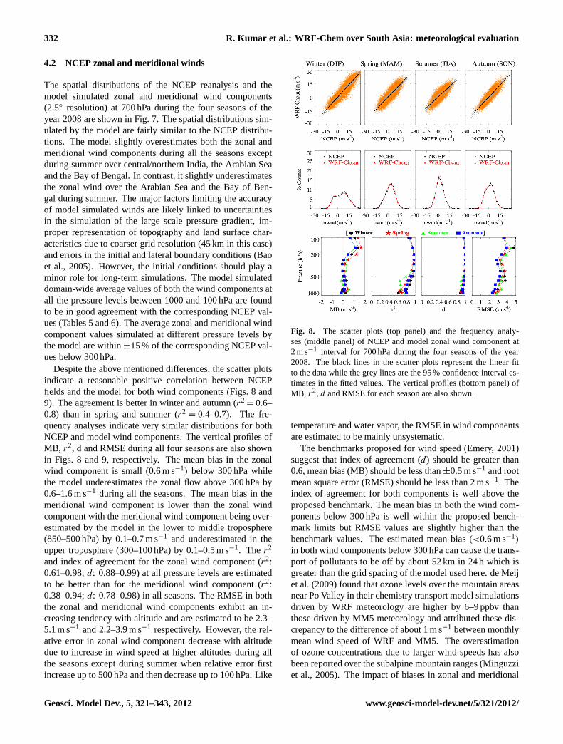
4.2 NCEP zonal and meridional winds
The spatial distributions of the NCEP reanalysis and themodel simulated zonal and meridional wind components(2.5◦ resolution) at 700 hPa during the four seasons of theyear 2008 are shown in Fig. 7. The spatial distributions sim-ulated by the model are fairly similar to the NCEP distribu-tions. The model slightly overestimates both the zonal andmeridional wind components during all the seasons exceptduring summer over central/northern India, the Arabian Seaand the Bay of Bengal. In contrast, it slightly underestimatesthe zonal wind over the Arabian Sea and the Bay of Ben-gal during summer. The major factors limiting the accuracyof model simulated winds are likely linked to uncertaintiesin the simulation of the large scale pressure gradient, im-proper representation of topography and land surface char-acteristics due to coarser grid resolution (45 km in this case)and errors in the initial and lateral boundary conditions (Baoet al., 2005). However, the initial conditions should play aminor role for long-term simulations. The model simulateddomain-wide average values of both the wind components atall the pressure levels between 1000 and 100 hPa are foundto be in good agreement with the corresponding NCEP val-ues (Tables 5 and 6). The average zonal and meridional windcomponent values simulated at different pressure levels bythe model are within±15 % of the corresponding NCEP val-ues below 300 hPa.
Despite the above mentioned differences, the scatter plotsindicate a reasonable positive correlation between NCEPfields and the model for both wind components (Figs. 8 and9). The agreement is better in winter and autumn (r2
= 0.6–0.8) than in spring and summer (r2
= 0.4–0.7). The fre-quency analyses indicate very similar distributions for bothNCEP and model wind components. The vertical profiles ofMB, r2, d and RMSE during all four seasons are also shownin Figs. 8 and 9, respectively. The mean bias in the zonalwind component is small (0.6 m s−1) below 300 hPa whilethe model underestimates the zonal flow above 300 hPa by0.6–1.6 m s−1 during all the seasons. The mean bias in themeridional wind component is lower than the zonal windcomponent with the meridional wind component being over-estimated by the model in the lower to middle troposphere(850–500 hPa) by 0.1–0.7 m s−1 and underestimated in theupper troposphere (300–100 hPa) by 0.1–0.5 m s−1. The r2
and index of agreement for the zonal wind component (r2:0.61–0.98;d: 0.88–0.99) at all pressure levels are estimatedto be better than for the meridional wind component (r2:0.38–0.94;d: 0.78–0.98) in all seasons. The RMSE in boththe zonal and meridional wind components exhibit an in-creasing tendency with altitude and are estimated to be 2.3–5.1 m s−1 and 2.2–3.9 m s−1 respectively. However, the rel-ative error in zonal wind component decrease with altitudedue to increase in wind speed at higher altitudes during allthe seasons except during summer when relative error firstincrease up to 500 hPa and then decrease up to 100 hPa. Like
Page 62 of 69
1035
Figure 8: The scatter plots (top panel) and the frequency analyses (middle panel) of NCEP and 1036
model zonal wind component at 2 m s-1 interval for 700 hPa during the four seasons of the year 1037
2008. The black lines in the scatter plots represent the linear fit to the data while the grey lines 1038
are the 95% confidence interval estimates in the fitted values. The vertical profiles (bottom 1039
panel) of MB, r2, d and RMSE for each season are also shown. 1040
Fig. 8. The scatter plots (top panel) and the frequency analy-ses (middle panel) of NCEP and model zonal wind component at2 m s−1 interval for 700 hPa during the four seasons of the year2008. The black lines in the scatter plots represent the linear fitto the data while the grey lines are the 95 % confidence interval es-timates in the fitted values. The vertical profiles (bottom panel) ofMB, r2, d and RMSE for each season are also shown.
temperature and water vapor, the RMSE in wind componentsare estimated to be mainly unsystematic.
The benchmarks proposed for wind speed (Emery, 2001)suggest that index of agreement (d) should be greater than0.6, mean bias (MB) should be less than±0.5 m s−1 and rootmean square error (RMSE) should be less than 2 m s−1. Theindex of agreement for both components is well above theproposed benchmark. The mean bias in both the wind com-ponents below 300 hPa is well within the proposed bench-mark limits but RMSE values are slightly higher than thebenchmark values. The estimated mean bias (<0.6 m s−1)
in both wind components below 300 hPa can cause the trans-port of pollutants to be off by about 52 km in 24 h which isgreater than the grid spacing of the model used here. de Meijet al. (2009) found that ozone levels over the mountain areasnear Po Valley in their chemistry transport model simulationsdriven by WRF meteorology are higher by 6–9 ppbv thanthose driven by MM5 meteorology and attributed these dis-crepancy to the difference of about 1 m s−1 between monthlymean wind speed of WRF and MM5. The overestimationof ozone concentrations due to larger wind speeds has alsobeen reported over the subalpine mountain ranges (Minguzziet al., 2005). The impact of biases in zonal and meridional
Geosci. Model Dev., 5, 321–343, 2012 www.geosci-model-dev.net/5/321/2012/
R. Kumar et al.: WRF-Chem over South Asia: meteorological evaluation 333
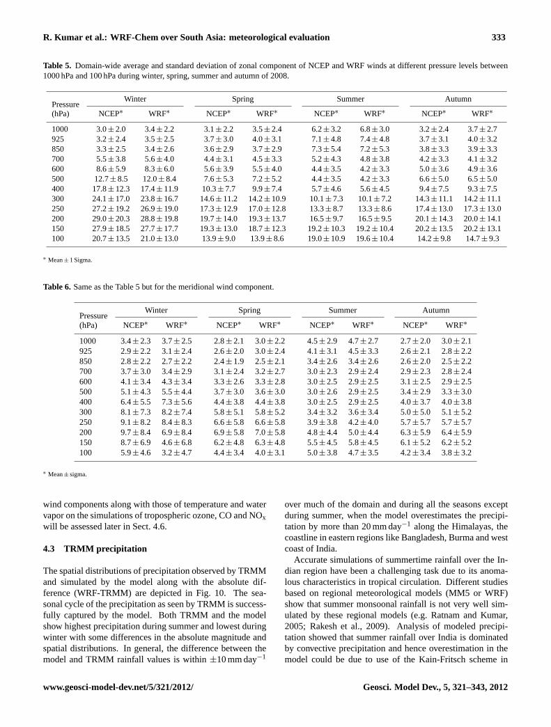
Table 5. Domain-wide average and standard deviation of zonal component of NCEP and WRF winds at different pressure levels between1000 hPa and 100 hPa during winter, spring, summer and autumn of 2008.
PressureWinter Spring Summer Autumn
(hPa) NCEP∗ WRF∗ NCEP∗ WRF∗ NCEP∗ WRF∗ NCEP∗ WRF∗
1000 3.0± 2.0 3.4± 2.2 3.1± 2.2 3.5± 2.4 6.2± 3.2 6.8± 3.0 3.2± 2.4 3.7± 2.7925 3.2± 2.4 3.5± 2.5 3.7± 3.0 4.0± 3.1 7.1± 4.8 7.4± 4.8 3.7± 3.1 4.0± 3.2850 3.3± 2.5 3.4± 2.6 3.6± 2.9 3.7± 2.9 7.3± 5.4 7.2± 5.3 3.8± 3.3 3.9± 3.3700 5.5± 3.8 5.6± 4.0 4.4± 3.1 4.5± 3.3 5.2± 4.3 4.8± 3.8 4.2± 3.3 4.1± 3.2600 8.6± 5.9 8.3± 6.0 5.6± 3.9 5.5± 4.0 4.4± 3.5 4.2± 3.3 5.0± 3.6 4.9± 3.6500 12.7± 8.5 12.0± 8.4 7.6± 5.3 7.2± 5.2 4.4± 3.5 4.2± 3.3 6.6± 5.0 6.5± 5.0400 17.8± 12.3 17.4± 11.9 10.3± 7.7 9.9± 7.4 5.7± 4.6 5.6± 4.5 9.4± 7.5 9.3± 7.5300 24.1± 17.0 23.8± 16.7 14.6± 11.2 14.2± 10.9 10.1± 7.3 10.1± 7.2 14.3± 11.1 14.2± 11.1250 27.2± 19.2 26.9± 19.0 17.3± 12.9 17.0± 12.8 13.3± 8.7 13.3± 8.6 17.4± 13.0 17.3± 13.0200 29.0± 20.3 28.8± 19.8 19.7± 14.0 19.3± 13.7 16.5± 9.7 16.5± 9.5 20.1± 14.3 20.0± 14.1150 27.9± 18.5 27.7± 17.7 19.3± 13.0 18.7± 12.3 19.2± 10.3 19.2± 10.4 20.2± 13.5 20.2± 13.1100 20.7± 13.5 21.0± 13.0 13.9± 9.0 13.9± 8.6 19.0± 10.9 19.6± 10.4 14.2± 9.8 14.7± 9.3
∗ Mean± 1 Sigma.
Table 6. Same as the Table 5 but for the meridional wind component.
PressureWinter Spring Summer Autumn
(hPa) NCEP∗ WRF∗ NCEP∗ WRF∗ NCEP∗ WRF∗ NCEP∗ WRF∗
1000 3.4± 2.3 3.7± 2.5 2.8± 2.1 3.0± 2.2 4.5± 2.9 4.7± 2.7 2.7± 2.0 3.0± 2.1925 2.9± 2.2 3.1± 2.4 2.6± 2.0 3.0± 2.4 4.1± 3.1 4.5± 3.3 2.6± 2.1 2.8± 2.2850 2.8± 2.2 2.7± 2.2 2.4± 1.9 2.5± 2.1 3.4± 2.6 3.4± 2.6 2.6± 2.0 2.5± 2.2700 3.7± 3.0 3.4± 2.9 3.1± 2.4 3.2± 2.7 3.0± 2.3 2.9± 2.4 2.9± 2.3 2.8± 2.4600 4.1± 3.4 4.3± 3.4 3.3± 2.6 3.3± 2.8 3.0± 2.5 2.9± 2.5 3.1± 2.5 2.9± 2.5500 5.1± 4.3 5.5± 4.4 3.7± 3.0 3.6± 3.0 3.0± 2.6 2.9± 2.5 3.4± 2.9 3.3± 3.0400 6.4± 5.5 7.3± 5.6 4.4± 3.8 4.4± 3.8 3.0± 2.5 2.9± 2.5 4.0± 3.7 4.0± 3.8300 8.1± 7.3 8.2± 7.4 5.8± 5.1 5.8± 5.2 3.4± 3.2 3.6± 3.4 5.0± 5.0 5.1± 5.2250 9.1± 8.2 8.4± 8.3 6.6± 5.8 6.6± 5.8 3.9± 3.8 4.2± 4.0 5.7± 5.7 5.7± 5.7200 9.7± 8.4 6.9± 8.4 6.9± 5.8 7.0± 5.8 4.8± 4.4 5.0± 4.4 6.3± 5.9 6.4± 5.9150 8.7± 6.9 4.6± 6.8 6.2± 4.8 6.3± 4.8 5.5± 4.5 5.8± 4.5 6.1± 5.2 6.2± 5.2100 5.9± 4.6 3.2± 4.7 4.4± 3.4 4.0± 3.1 5.0± 3.8 4.7± 3.5 4.2± 3.4 3.8± 3.2
∗ Mean± sigma.
wind components along with those of temperature and watervapor on the simulations of tropospheric ozone, CO and NOxwill be assessed later in Sect. 4.6.
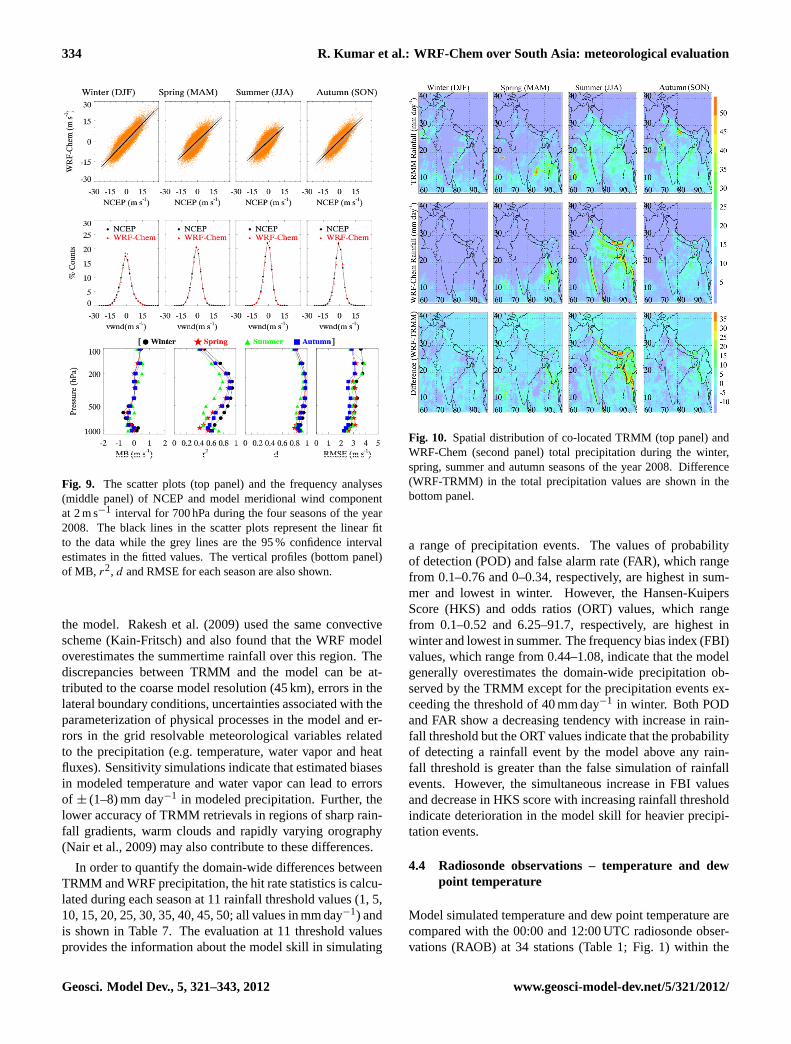
4.3 TRMM precipitation
The spatial distributions of precipitation observed by TRMMand simulated by the model along with the absolute dif-ference (WRF-TRMM) are depicted in Fig. 10. The sea-sonal cycle of the precipitation as seen by TRMM is success-fully captured by the model. Both TRMM and the modelshow highest precipitation during summer and lowest duringwinter with some differences in the absolute magnitude andspatial distributions. In general, the difference between themodel and TRMM rainfall values is within±10 mm day−1
over much of the domain and during all the seasons exceptduring summer, when the model overestimates the precipi-tation by more than 20 mm day−1 along the Himalayas, thecoastline in eastern regions like Bangladesh, Burma and westcoast of India.
Accurate simulations of summertime rainfall over the In-dian region have been a challenging task due to its anoma-lous characteristics in tropical circulation. Different studiesbased on regional meteorological models (MM5 or WRF)show that summer monsoonal rainfall is not very well sim-ulated by these regional models (e.g. Ratnam and Kumar,2005; Rakesh et al., 2009). Analysis of modeled precipi-tation showed that summer rainfall over India is dominatedby convective precipitation and hence overestimation in themodel could be due to use of the Kain-Fritsch scheme in
www.geosci-model-dev.net/5/321/2012/ Geosci. Model Dev., 5, 321–343, 2012
334 R. Kumar et al.: WRF-Chem over South Asia: meteorological evaluation
Page 63 of 69
1041
Figure 9: The scatter plots (top panel) and the frequency analyses (middle panel) of NCEP and 1042
model meridional wind component at 2 m s-1 interval for 700 hPa during the four seasons of the 1043
year 2008. The black lines in the scatter plots represent the linear fit to the data while the grey 1044
lines are the 95% confidence interval estimates in the fitted values. The vertical profiles (bottom 1045
panel) of MB, r2, d and RMSE for each season are also shown. 1046
Fig. 9. The scatter plots (top panel) and the frequency analyses(middle panel) of NCEP and model meridional wind componentat 2 m s−1 interval for 700 hPa during the four seasons of the year2008. The black lines in the scatter plots represent the linear fitto the data while the grey lines are the 95 % confidence intervalestimates in the fitted values. The vertical profiles (bottom panel)of MB, r2, d and RMSE for each season are also shown.
the model. Rakesh et al. (2009) used the same convectivescheme (Kain-Fritsch) and also found that the WRF modeloverestimates the summertime rainfall over this region. Thediscrepancies between TRMM and the model can be at-tributed to the coarse model resolution (45 km), errors in thelateral boundary conditions, uncertainties associated with theparameterization of physical processes in the model and er-rors in the grid resolvable meteorological variables relatedto the precipitation (e.g. temperature, water vapor and heatfluxes). Sensitivity simulations indicate that estimated biasesin modeled temperature and water vapor can lead to errorsof ± (1–8) mm day−1 in modeled precipitation. Further, thelower accuracy of TRMM retrievals in regions of sharp rain-fall gradients, warm clouds and rapidly varying orography(Nair et al., 2009) may also contribute to these differences.
In order to quantify the domain-wide differences betweenTRMM and WRF precipitation, the hit rate statistics is calcu-lated during each season at 11 rainfall threshold values (1, 5,10, 15, 20, 25, 30, 35, 40, 45, 50; all values in mm day−1) andis shown in Table 7. The evaluation at 11 threshold valuesprovides the information about the model skill in simulating
Fig. 10. Spatial distribution of co-located TRMM (top panel) andWRF-Chem (second panel) total precipitation during the winter,spring, summer and autumn seasons of the year 2008. Difference(WRF-TRMM) in the total precipitation values are shown in thebottom panel.
a range of precipitation events. The values of probabilityof detection (POD) and false alarm rate (FAR), which rangefrom 0.1–0.76 and 0–0.34, respectively, are highest in sum-mer and lowest in winter. However, the Hansen-KuipersScore (HKS) and odds ratios (ORT) values, which rangefrom 0.1–0.52 and 6.25–91.7, respectively, are highest inwinter and lowest in summer. The frequency bias index (FBI)values, which range from 0.44–1.08, indicate that the modelgenerally overestimates the domain-wide precipitation ob-served by the TRMM except for the precipitation events ex-ceeding the threshold of 40 mm day−1 in winter. Both PODand FAR show a decreasing tendency with increase in rain-fall threshold but the ORT values indicate that the probabilityof detecting a rainfall event by the model above any rain-fall threshold is greater than the false simulation of rainfallevents. However, the simultaneous increase in FBI valuesand decrease in HKS score with increasing rainfall thresholdindicate deterioration in the model skill for heavier precipi-tation events.
4.4 Radiosonde observations – temperature and dewpoint temperature
Model simulated temperature and dew point temperature arecompared with the 00:00 and 12:00 UTC radiosonde obser-vations (RAOB) at 34 stations (Table 1; Fig. 1) within the
Geosci. Model Dev., 5, 321–343, 2012 www.geosci-model-dev.net/5/321/2012/

R. Kumar et al.: WRF-Chem over South Asia: meteorological evaluation 335
Table 7. Hit rate statistics (probability of detection (POD), false alarm rate (FAR), frequency bias (FBI), Hansen-Kuipers Score (HKS)and odd ratio (ORT)) for WRF-Chem and TRMM daily precipitation data during winter, spring, summer and autumn at different thresholdvalues.
SeasonThreshold Precipitation (mm day−1)
1 5 10 15 20 25 30 35 40 45 50
POD
Winter 0.59 0.55 0.51 0.46 0.40 0.35 0.30 0.25 0.20 0.14 0.10Spring 0.62 0.55 0.49 0.44 0.40 0.36 0.32 0.29 0.25 0.22 0.18Summer 0.76 0.67 0.60 0.54 0.49 0.44 0.39 0.34 0.30 0.26 0.22Autumn 0.67 0.61 0.56 0.51 0.45 0.40 0.35 0.30 0.26 0.22 0.18
FAR
Winter 0.09 0.04 0.03 0.02 0.01 0.01 0.01 0.01 0.00 0.00 0.00Spring 0.15 0.09 0.06 0.05 0.04 0.03 0.02 0.02 0.01 0.01 0.01Summer 0.34 0.25 0.19 0.16 0.13 0.10 0.08 0.06 0.05 0.04 0.03Autumn 0.14 0.10 0.08 0.06 0.05 0.04 0.03 0.02 0.01 0.01 0.01
FBI
Winter 0.60 0.64 0.62 0.62 0.65 0.70 0.76 0.86 1.02 1.30 1.80Spring 0.72 0.65 0.60 0.57 0.56 0.55 0.56 0.58 0.62 0.67 0.73Summer 0.69 0.60 0.52 0.48 0.46 0.44 0.45 0.46 0.47 0.50 0.54Autumn 0.78 0.70 0.65 0.63 0.63 0.65 0.68 0.72 0.79 0.88 1.00
HKS
Winter 0.50 0.51 0.48 0.44 0.39 0.34 0.29 0.25 0.20 0.14 0.10Spring 0.48 0.46 0.43 0.39 0.36 0.33 0.30 0.27 0.24 0.21 0.18Summer 0.42 0.43 0.41 0.39 0.37 0.34 0.31 0.28 0.25 0.22 0.19Autumn 0.52 0.51 0.48 0.45 0.41 0.36 0.32 0.28 0.24 0.21 0.17
ORT
Winter 14.2 27.3 37.3 44.3 49.6 55.6 62.0 70.2 79.4 84.2 91.7Spring 9.6 12.5 14.6 16.2 18.1 20.4 22.7 25.3 28.2 31.4 34.9Summer 6.3 6.3 6.2 6.4 6.7 7.1 7.4 7.9 8.6 9.4 10.2Autumn 12.0 14.1 15.2 16.2 17.0 18.3 19.8 21.6 23.6 26.6 29.5
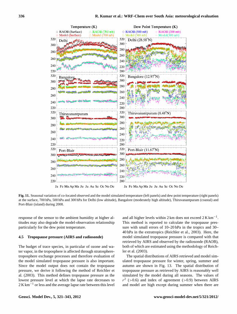
simulation domain. The seasonal variations of the RAOBand the model simulated temperature and dew point tem-perature at the surface, 700 hPa, 500 hPa and 300 hPa forDelhi (DEL), Bangalore (BAN), Thiruvanantpuram (THI)and Port-Blair (POR) are shown in Fig. 11. DEL, BAN, THIand POR are selected to represent the low altitude, moder-ately high altitude, coastal and island sites respectively. Ingeneral, the seasonal variations of both the temperature anddew point temperature simulated by the model at all the pres-sure levels are in reasonably good agreement with the obser-vations. Some differences between model and observed val-ues of the dew point temperature are seen at higher altitudes.The discrepancies for dew point temperature are consistentwith the model-AIRS water vapor comparison for which anincrease in RMSE is seen with altitude (Fig. 6). Port Blair,an island site, shows some differences at surface levels as themodel is not able to separate out island with the oceanic re-gion; this will be discussed later in this section. Like AIRSretrievals, RAOB observations also show differences in theseasonal cycle amplitude for the sites located north and southof the 20◦ N latitude belt. The seasonal amplitudes at DELare clearly larger than those at BAN, THI and POR and thisdifference is also very well replicated by the model.
Figure 12 shows the vertical profiles of the statistical met-rics for the temperature and dew point temperature at all thesites belonging to the low altitude, moderately high altitude,
coastal and island sites respectively. The correlation (r2) isbetter for temperature for the case of low altitude and moder-ately high altitude sites below 300 hPa. The poorer correla-tion at the coastal and island sites appears to be largely due tothe erroneous model representation of the underlying surfaceat these sites. An examination of the land-use categories usedby the model indicates that all three island sites (AMI, MINand POR) and the six coastal sites (BOM, GOA, PAN, COC,THI and VIS) are treated as “water bodies” by the model andthe other four coastal sites (BHU, MAC, MAD and KAR)are treated as “Irrigated Cropland and Pasture”. The differ-ences between the true and the model topography may alsocontribute to errors in the model simulated temperature. Theactual altitudes of the site along with the altitude used by themodel are shown in the Table 1. The difference in the trueand the model topography is less than 250 m for all the sitesand is less than 50 m for 26 out of the 34 sites consideredhere.
The MB, RMSE, RMSEs and RMSEu show a gradual in-crease in magnitude with altitude. For all the site categories,average values of MB, RMSE, RMSEs and RMSEu are lowerfor the temperature (0.2–7 K) compared to dew point temper-ature profiles (0.1–10 K).Systematic errors contribute moreto RMSE between the model and in situ observations. Apartfrom the model, the errors in the radiosonde water vapormeasurements due to reduced water vapor amount and slower
www.geosci-model-dev.net/5/321/2012/ Geosci. Model Dev., 5, 321–343, 2012
336 R. Kumar et al.: WRF-Chem over South Asia: meteorological evaluation
Fig. 11.Seasonal variation of co-located observed and the model simulated temperature (left panels) and dew point temperature (right panels)at the surface, 700 hPa, 500 hPa and 300 hPa for Delhi (low altitude), Bangalore (moderately high altitude), Thiruvanantpuram (coastal) andPort-Blair (island) during 2008.
response of the sensor to the ambient humidity at higher al-titudes may also degrade the model-observation relationshipparticularly for the dew point temperature.
4.5 Tropopause pressure (AIRS and radiosonde)
The budget of trace species, in particular of ozone and wa-ter vapor, in the troposphere is affected through stratosphere-troposphere exchange processes and therefore evaluation ofthe model simulated tropopause pressure is also important.Since the model output does not contain the tropopausepressure, we derive it following the method of Reichler etal. (2003). This method defines tropopause pressure as thelowest pressure level at which the lapse rate decreases to2 K km−1 or less and the average lapse rate between this level
and all higher levels within 2 km does not exceed 2 K km−1.This method is reported to calculate the tropopause pres-sure with small errors of 10–20 hPa in the tropics and 30–40 hPa in the extratropics (Reichler et al., 2003). Here, themodel simulated tropopause pressure is compared with thatretrieved by AIRS and observed by the radiosonde (RAOB),both of which are estimated using the methodology of Reich-ler et al. (2003).
The spatial distributions of AIRS retrieved and model sim-ulated tropopause pressure for winter, spring, summer andautumn are shown in Fig. 13. The spatial distribution oftropopause pressure as retrieved by AIRS is reasonably wellsimulated by the model during all seasons. The values ofr2 (>0.6) and index of agreement (>0.9) between AIRSand model are high except during summer when there are
Geosci. Model Dev., 5, 321–343, 2012 www.geosci-model-dev.net/5/321/2012/

R. Kumar et al.: WRF-Chem over South Asia: meteorological evaluation 337
Fig. 12. Vertical profiles of the statistical metrics for temperature (top panel) and dew point temperature (bottom panel) at all the sitesbelonging to low altitude, moderate altitude, coastal and island sites. Average profiles of the statistical metrics for each site category arealso shown. The dotted lines represent the profiles for individual sites and solid lines connected by symbols represent the respective averageprofiles.
fewer clear-sky observations and a smaller set of observa-tions available. Both AIRS and model tropopause pressureshow a distinct seasonal cycle with highest tropopause pres-sure in summer (90–100 hPa) and lowest in winter (120–270 hPa) over the regions located north of 30◦ N latitude belt.South of 30◦ N the seasonal amplitude is small (10–20 hPa).The latitudinal variation in tropopause pressure can be at-tributed to the seasonal variability in solar radiation at thesub-tropical latitudes.
The differences between AIRS and the model tropopausepressure can be discerned over the topographically complexHimalayan region. The mean bias values in the model simu-lated tropopause pressure as compared to the AIRS retrievalsare estimated as 1 hPa,−9 hPa, 2 hPa and 5 hPa for the fourseasons, respectively and the corresponding RMSE valuesare 36, 36, 24 and 25 hPa, respectively. These differencesover the Himalayan region could be attributed to the errors inthe simulated temperature profiles associated with improperrepresentation of surface topography in the model and thetopography induced errors in the satellite retrievals.
Apart from evaluation with AIRS retrievals, the errors inWRF-Chem simulated tropopause pressure are also quanti-fied by comparing the model results with RAOB datasets.The annual average values of the RAOB and the modelestimated tropopause pressure values for the defined foursite categories are shown in Table 8, which also shows thecomparison of WRF-Chem and AIRS tropopause pressurefor the four site categories. Mean WRF-Chem and AIRStropopause pressure values are estimated by averaging theco-located data points over a 0.25◦
× 0.25◦ box centered atthe geographical location of a RAOB site. The annual av-erage tropopause pressure values in WRF-Chem and AIRSare estimated to be around 98–103 hPa as compared to theRAOB values of 115–120 hPa. The MB and RMSE in themodel estimated tropopause pressure values with respect tothe corresponding RAOB values are estimated to be 14–17 hPa and 19–23 hPa respectively (Table 8) while the re-spective values resulting from comparison with AIRS are−1to −3 hPa and 3–22 hPa respectively. By having an accu-rately placed tropopause, stratosphere-troposphere exchange
www.geosci-model-dev.net/5/321/2012/ Geosci. Model Dev., 5, 321–343, 2012

338 R. Kumar et al.: WRF-Chem over South Asia: meteorological evaluation
60E 70E 80E 90E 100E
10N
20N
30N
40N
Winter (DJF)
60E 70E 80E 90E 100E
10N
20N
30N
40N
60E 70E 80E 90E 100E
10N
20N
30N
40N
Spring (MAM)
60E 70E 80E 90E 100E
10N
20N
30N
40N
60E 70E 80E 90E 100E
10N
20N
30N
40N
Summer (JJA)
60E 70E 80E 90E 100E
10N
20N
30N
40N
60E 70E 80E 90E 100E
10N
20N
30N
40N
Autumn (SON)
90105120135150165180195210225240450
60E 70E 80E 90E 100E
10N
20N
30N
40N
90105120135150165180195210225240450
Fig. 13. Spatial distribution of co-located AIRS retrieved (top panel) and model simulated (bottom panel) tropopause pressure during thewinter, spring, summer and autumn seasons of the year 2008.
Table 8. Annual average and standard deviation in co-located RAOB and WRF-Chem tropopause pressures for the four site categoriesdefined in this study are shown along with mean bias and the root mean square error. All these statistical parameters are also shown forco-located AIRS and WRF-Chem tropopause pressure values. All the values are rounded off to their nearest integer values.
Site CategoryWRF-Chem vs. RAOB Tropopause Pressure (hPa) WRF-Chem vs. AIRS Tropopause Pressure (hPa)
RAOB WRF-Chem MB RMSE AIRS WRF-Chem MB RMSE
Low Altitude 115± 14 101± 8 14 21 101± 21 103± 18 −2 22Moderately High Altitude 115± 12 100± 2 15 19 98± 4 99± 2 −2 4Coastal 118± 13 102± 2 16 21 100± 18 101± 2 −1 18Island 120± 15 103± 2 17 23 99± 2 102± 2 −3 3
processes should be reasonably represented. This is particu-larly important for the Himalayan region.
4.6 Sensitivity simulations
The possible impacts of estimated errors in meteorologicalparameters on the simulations of chemical species concentra-tions were discussed qualitatively and individually for eachparameter in the previous sections. This section presents theresults from sensitivity simulations conducted to quantify theerrors in chemistry simulations by combining the errors in
meteorological parameters. The initial and boundary condi-tions for temperature, water vapor and wind components aremodified by adding highest MB value, identified by compar-ing MB profiles of all the four seasons, of the respective me-teorological parameter at each level between 1000 hPa and100 hPa and 10-days runs are conducted during May and July(representing the months of dry and wet weather conditions).The MB profiles used for perturbation of meteorological pa-rameters are shown in Table 9. It is to be noted that emissionsof trace gases and aerosols are not changed from the basemodel run values for these sensitivity runs. The percentage
Geosci. Model Dev., 5, 321–343, 2012 www.geosci-model-dev.net/5/321/2012/

R. Kumar et al.: WRF-Chem over South Asia: meteorological evaluation 339
Table 9. Vertical profiles of mean bias in temperature, water vapor and wind components used to modify the initial and boundary conditionsof these meteorological variables between 1000 and 100 hPa for sensitivity simulations. Note that mean bias profiles for water vapor areestimated only up to 300 hPa.
Pressure Temperature Water Vapor Zonal Wind Meridional Wind(hPa) (K) (%) (m s−1) (m s−1)
1000 1.4 −6.7 0.23 −0.40925 −1.4 13.9 0.40 0.25850 −0.4 −17.1 0.57 −0.47700 −0.3 −16.8 0.20 −0.55600 −0.8 −5.7 0.31 −0.70500 −1.3 −14.3 0.15 −0.36400 −0.8 −15.0 0.27 −0.05300 −0.7 −32.0 0.32 0.11250 −1.2 − 0.34 0.27200 −1.2 − 1.22 0.51150 −1.5 − 1.64 0.54100 −1.8 − 1.37 0.44
differences in model simulated tropospheric column ozone,CO and NOx between sensitivity and base model runs arecalculated for each grid point and are shown in Fig. 14. Ingeneral, the percentage differences in tropospheric columnozone and CO are within±10 % while those in NOx are ashigh as 25 % for some of the grid points. The largest dif-ferences in tropospheric column NOx are seen over partsof Indo-Gangetic Plain, southern tip of India and along theeastern Indian coast. Since these simulations do not includelightning-NOx parametrization, these differences cannot beattributed to lightning-NOx process.
In order to understand the reasons for larger differences intropospheric NOx distributions, model simulated precipita-tion from sensitivity and base runs are analyzed along withspatial distributions of ozone, CO and NOx at four differentpressure levels (850 hPa, 700 hPa, 500 hPa and 300 hPa). Thespatial distributions of percentage differences in model simu-lated ozone, CO and NOx at 850 and 500 hPa during May andJuly are shown in Fig. 15. Perturbation in meteorological pa-rameters causes the percentage differences in ozone and COwithin ±20 % at different pressure levels. It is found that per-turbations in meteorological parameters increase NOx lev-els by more 60–100 % in the lower atmosphere and decreasethem by 0–40 % in the middle and upper troposphere. Sim-ilar enhancement in the lower atmosphere and decrease inmiddle-upper troposphere is also observed for model simu-lated nitric acid (HNO3) and formaldehyde (HCHO) values.Analysis of modeled precipitation reveals that areas of en-hanced NOx, HNO3 and HCHO levels are associated withreduced precipitation. The reduction in precipitation resultsin a longer HNO3 lifetime allowing it to transform back toNOx via photolysis.
Fig. 14. Spatial distributions of percentage differences in modelsimulated tropospheric column ozone, CO and NOx between sensi-tivity and base model runs during May and July 2008.
5 Summary and discussions
The Weather Research and Forecasting model coupled withChemistry (WRF-Chem) has been set-up over the SouthAsian region and has been used, for the first time, to sim-ulate a full year (2008). In this manuscript, the meteo-rological parameters simulated by the model are evaluatedthrough comparison with a variety of datasets including ra-diosonde observations of temperature, dew point temperatureand tropopause pressure, AIRS retrievals of temperature, wa-ter vapor and tropopause pressure, NCEP reanalysis zonaland meridional wind components and TRMM derived daily
www.geosci-model-dev.net/5/321/2012/ Geosci. Model Dev., 5, 321–343, 2012

340 R. Kumar et al.: WRF-Chem over South Asia: meteorological evaluation
Fig. 15. Spatial distributions of percentage differences in ozone,CO and NOx at 850 and 500 hPa between sensitivity and base modelruns during May and July 2008. White space in the top two panelsindicates the regions of surface pressure lower than 850 hPa.
precipitation. The model results are co-located in both spaceand time with the quality-controlled observed data for propercomparison. The model successfully replicated the generalfeatures of the South Asian meteorology such as the sea-sonal changes in wind patterns along with the seasonal cy-cle of temperature, water vapor, precipitation and tropopausepressure. All these meteorological parameters showed a dis-tinct seasonal cycle with highest values (altitude in case oftropopause pressure) in summer and lowest during winter.
The model-observation relationship and the errors in themodel simulated parameters are quantified using differentstatistical metrics. The statistics obtained by this comparisonindicate that the agreement between model and observationsis better for temperature as compared to the other parame-ters. The model is biased cold near the surface in all theseasons while it is biased warm aloft with MB and RMSE
values within±2 K and 1–4 K, respectively. Both MB andRMSE in temperature are estimated to be higher at the sur-face and lower at upper levels. On average, the model isbiased dry at 1000 hPa in winter and spring while it is bi-ased wet at this level in summer and autumn with MB andRMSE values less than 20 %. The mean bias and RMSEin water vapor at upper pressure levels range between 20–30 % and 20–65 %, respectively. The model simulated windsshow both an easterly and a northerly bias. RMSE in zonaland meridional wind components are estimated to be 2.3–5.1 m s−1 and 2.2–3.9 m s−1, respectively. MB and RMSEin wind components increase gradually with altitude. Thespatial and temporal variability of rainfall events is also cap-tured reasonably well by the model as indicated by higherodd ratio values (6–92). The frequency bias index values in-dicate that the model generally overestimates domain-wideprecipitation except for some events exceeding 40 mm day−1
in winter.The radiosonde observations are classified into low alti-
tude, moderately high altitude, coastal and island sites. Theseasonal variability of temperature and dew point tempera-ture for these four categories is replicated well by the model.However, estimated statistical metrics indicate relatively bet-ter result for inland sites as compared to coastal and islandsites. Analysis of the topography and land-cover used by themodel suggest that erroneous representation of these surfacecharacteristics possibly due in parts to the coarse model res-olution (45 km) leads to a poorer correlation for these sites.The spatio-temporal variability of tropopause pressure is alsosimulated well by the model with mean bias and RMSE val-ues less than 25 hPa.
The statistical metrics estimated for temperature, watervapor and wind components are also compared with a setof proposed benchmarks to assess the implications of errorsin these parameters for chemistry simulations. In general,the errors in model simulated meteorological parameters arewell within or comparable to the proposed benchmark valuesand comparison with other studies showed that the errors inthese parameters should induce only small errors in chem-istry simulations. The errors in simulations of troposphericozone, CO and NOx due to biases in simulations of temper-ature, water vapor and wind components are estimated to bewithin ± (10–25 %). Overall, the model has good ability tosimulate the spatio-temporal variabilities of meteorologicalparameters over this region and would be of sufficient qual-ity for use in chemical transport modeling.
Acknowledgements.M. Naja and R. Kumar are thankful toShyam Lal, Ram Sagar and C. B. S. Dutt for their keeninterest in this work and acknowledge support from ISRO-ATCTM project. The meteorological datasets for initialand boundary conditions are downloaded from the websitehttp://dss.ucar.edu/datasets/ds083.2/data/. Radiosonde data areretrieved from the websitehttp://www.esrl.noaa.gov/raobs/.NCEP/NCAR reanalysis datasets are downloaded from theirwebsite athttp://www.esrl.noaa.gov/. The National Center for
Geosci. Model Dev., 5, 321–343, 2012 www.geosci-model-dev.net/5/321/2012/
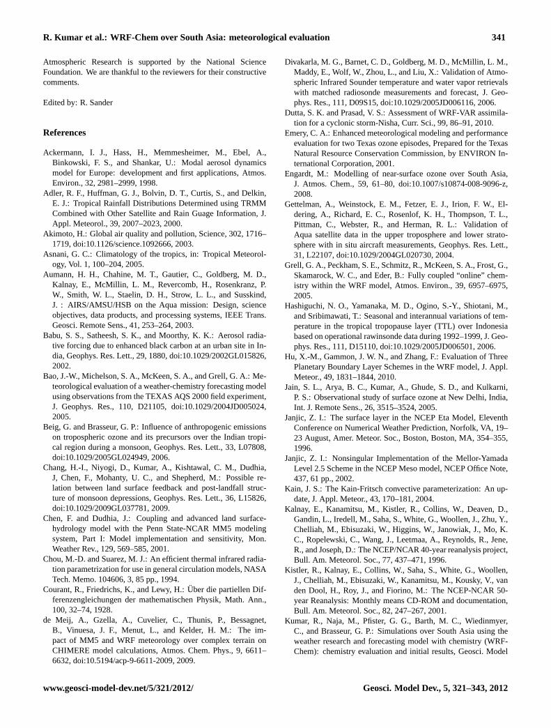
R. Kumar et al.: WRF-Chem over South Asia: meteorological evaluation 341
Atmospheric Research is supported by the National ScienceFoundation. We are thankful to the reviewers for their constructivecomments.
Edited by: R. Sander
References
Ackermann, I. J., Hass, H., Memmesheimer, M., Ebel, A.,Binkowski, F. S., and Shankar, U.: Modal aerosol dynamicsmodel for Europe: development and first applications, Atmos.Environ., 32, 2981–2999, 1998.
Adler, R. F., Huffman, G. J., Bolvin, D. T., Curtis, S., and Delkin,E. J.: Tropical Rainfall Distributions Determined using TRMMCombined with Other Satellite and Rain Guage Information, J.Appl. Meteorol., 39, 2007–2023, 2000.
Akimoto, H.: Global air quality and pollution, Science, 302, 1716–1719,doi:10.1126/science.1092666, 2003.
Asnani, G. C.: Climatology of the tropics, in: Tropical Meteorol-ogy, Vol. 1, 100–204, 2005.
Aumann, H. H., Chahine, M. T., Gautier, C., Goldberg, M. D.,Kalnay, E., McMillin, L. M., Revercomb, H., Rosenkranz, P.W., Smith, W. L., Staelin, D. H., Strow, L. L., and Susskind,J. : AIRS/AMSU/HSB on the Aqua mission: Design, scienceobjectives, data products, and processing systems, IEEE Trans.Geosci. Remote Sens., 41, 253–264, 2003.
Babu, S. S., Satheesh, S. K., and Moorthy, K. K.: Aerosol radia-tive forcing due to enhanced black carbon at an urban site in In-dia, Geophys. Res. Lett., 29, 1880,doi:10.1029/2002GL015826,2002.
Bao, J.-W., Michelson, S. A., McKeen, S. A., and Grell, G. A.: Me-teorological evaluation of a weather-chemistry forecasting modelusing observations from the TEXAS AQS 2000 field experiment,J. Geophys. Res., 110, D21105,doi:10.1029/2004JD005024,2005.
Beig, G. and Brasseur, G. P.: Influence of anthropogenic emissionson tropospheric ozone and its precursors over the Indian tropi-cal region during a monsoon, Geophys. Res. Lett., 33, L07808,doi:10.1029/2005GL024949, 2006.
Chang, H.-I., Niyogi, D., Kumar, A., Kishtawal, C. M., Dudhia,J, Chen, F., Mohanty, U. C., and Shepherd, M.: Possible re-lation between land surface feedback and post-landfall struc-ture of monsoon depressions, Geophys. Res. Lett., 36, L15826,doi:10.1029/2009GL037781, 2009.
Chen, F. and Dudhia, J.: Coupling and advanced land surface-hydrology model with the Penn State-NCAR MM5 modelingsystem, Part I: Model implementation and sensitivity, Mon.Weather Rev., 129, 569–585, 2001.
Chou, M.-D. and Suarez, M. J.: An efficient thermal infrared radia-tion parametrization for use in general circulation models, NASATech. Memo. 104606, 3, 85 pp., 1994.
Courant, R., Friedrichs, K., and Lewy, H.:Uber die partiellen Dif-ferenzengleichungen der mathematischen Physik, Math. Ann.,100, 32–74, 1928.
de Meij, A., Gzella, A., Cuvelier, C., Thunis, P., Bessagnet,B., Vinuesa, J. F., Menut, L., and Kelder, H. M.: The im-pact of MM5 and WRF meteorology over complex terrain onCHIMERE model calculations, Atmos. Chem. Phys., 9, 6611–6632,doi:10.5194/acp-9-6611-2009, 2009.
Divakarla, M. G., Barnet, C. D., Goldberg, M. D., McMillin, L. M.,Maddy, E., Wolf, W., Zhou, L., and Liu, X.: Validation of Atmo-spheric Infrared Sounder temperature and water vapor retrievalswith matched radiosonde measurements and forecast, J. Geo-phys. Res., 111, D09S15,doi:10.1029/2005JD006116, 2006.
Dutta, S. K. and Prasad, V. S.: Assessment of WRF-VAR assimila-tion for a cyclonic storm-Nisha, Curr. Sci., 99, 86–91, 2010.
Emery, C. A.: Enhanced meteorological modeling and performanceevaluation for two Texas ozone episodes, Prepared for the TexasNatural Resource Conservation Commission, by ENVIRON In-ternational Corporation, 2001.
Engardt, M.: Modelling of near-surface ozone over South Asia,J. Atmos. Chem., 59, 61–80,doi:10.1007/s10874-008-9096-z,2008.
Gettelman, A., Weinstock, E. M., Fetzer, E. J., Irion, F. W., El-dering, A., Richard, E. C., Rosenlof, K. H., Thompson, T. L.,Pittman, C., Webster, R., and Herman, R. L.: Validation ofAqua satellite data in the upper troposphere and lower strato-sphere with in situ aircraft measurements, Geophys. Res. Lett.,31, L22107,doi:10.1029/2004GL020730, 2004.
Grell, G. A., Peckham, S. E., Schmitz, R., McKeen, S. A., Frost, G.,Skamarock, W. C., and Eder, B.: Fully coupled “online” chem-istry within the WRF model, Atmos. Environ., 39, 6957–6975,2005.
Hashiguchi, N. O., Yamanaka, M. D., Ogino, S.-Y., Shiotani, M.,and Sribimawati, T.: Seasonal and interannual variations of tem-perature in the tropical tropopause layer (TTL) over Indonesiabased on operational rawinsonde data during 1992–1999, J. Geo-phys. Res., 111, D15110,doi:10.1029/2005JD006501, 2006.
Hu, X.-M., Gammon, J. W. N., and Zhang, F.: Evaluation of ThreePlanetary Boundary Layer Schemes in the WRF model, J. Appl.Meteor., 49, 1831–1844, 2010.
Jain, S. L., Arya, B. C., Kumar, A., Ghude, S. D., and Kulkarni,P. S.: Observational study of surface ozone at New Delhi, India,Int. J. Remote Sens., 26, 3515–3524, 2005.
Janjic, Z. I.: The surface layer in the NCEP Eta Model, EleventhConference on Numerical Weather Prediction, Norfolk, VA, 19–23 August, Amer. Meteor. Soc., Boston, Boston, MA, 354–355,1996.
Janjic, Z. I.: Nonsingular Implementation of the Mellor-YamadaLevel 2.5 Scheme in the NCEP Meso model, NCEP Office Note,437, 61 pp., 2002.
Kain, J. S.: The Kain-Fritsch convective parameterization: An up-date, J. Appl. Meteor., 43, 170–181, 2004.
Kalnay, E., Kanamitsu, M., Kistler, R., Collins, W., Deaven, D.,Gandin, L., Iredell, M., Saha, S., White, G., Woollen, J., Zhu, Y.,Chelliah, M., Ebisuzaki, W., Higgins, W., Janowiak, J., Mo, K.C., Ropelewski, C., Wang, J., Leetmaa, A., Reynolds, R., Jene,R., and Joseph, D.: The NCEP/NCAR 40-year reanalysis project,Bull. Am. Meteorol. Soc., 77, 437–471, 1996.
Kistler, R., Kalnay, E., Collins, W., Saha, S., White, G., Woollen,J., Chelliah, M., Ebisuzaki, W., Kanamitsu, M., Kousky, V., vanden Dool, H., Roy, J., and Fiorino, M.: The NCEP-NCAR 50-year Reanalysis: Monthly means CD-ROM and documentation,Bull. Am. Meteorol. Soc., 82, 247–267, 2001.
Kumar, R., Naja, M., Pfister, G. G., Barth, M. C., Wiedinmyer,C., and Brasseur, G. P.: Simulations over South Asia using theweather research and forecasting model with chemistry (WRF-Chem): chemistry evaluation and initial results, Geosci. Model
www.geosci-model-dev.net/5/321/2012/ Geosci. Model Dev., 5, 321–343, 2012
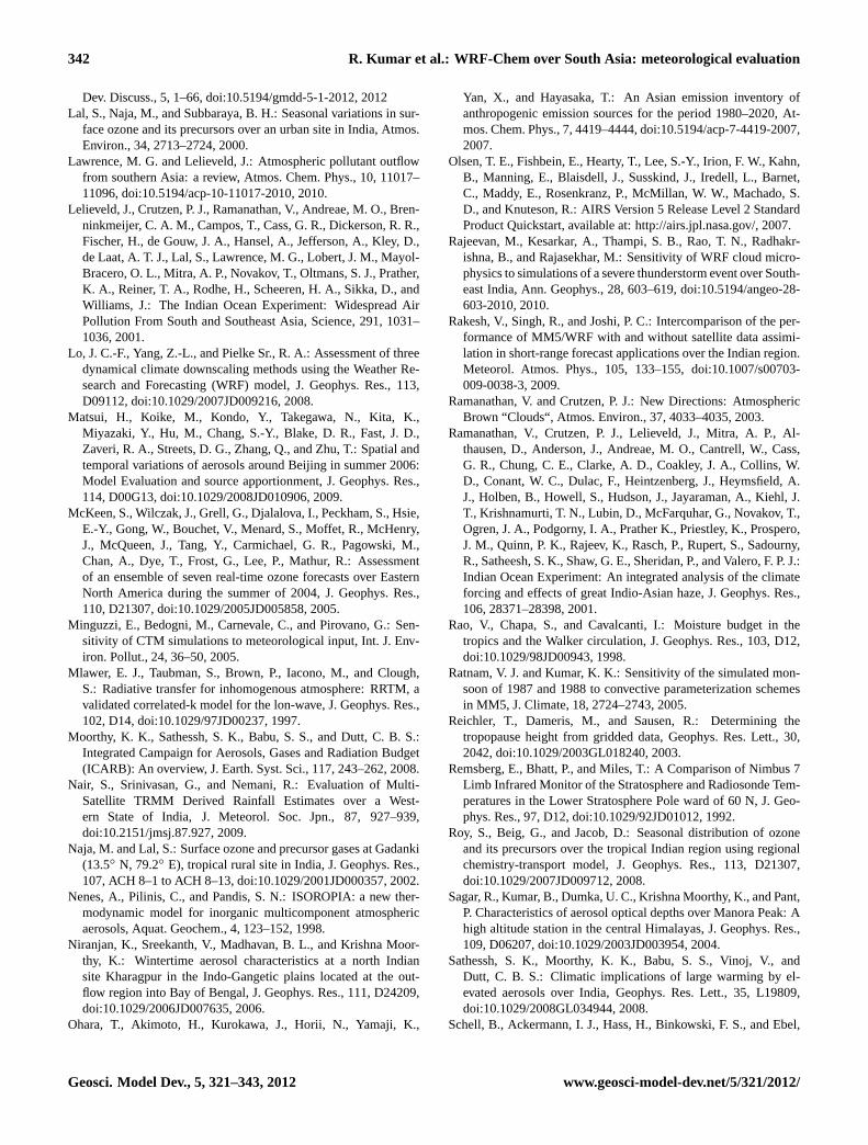
342 R. Kumar et al.: WRF-Chem over South Asia: meteorological evaluation
Dev. Discuss., 5, 1–66,doi:10.5194/gmdd-5-1-2012, 2012Lal, S., Naja, M., and Subbaraya, B. H.: Seasonal variations in sur-
face ozone and its precursors over an urban site in India, Atmos.Environ., 34, 2713–2724, 2000.
Lawrence, M. G. and Lelieveld, J.: Atmospheric pollutant outflowfrom southern Asia: a review, Atmos. Chem. Phys., 10, 11017–11096,doi:10.5194/acp-10-11017-2010, 2010.
Lelieveld, J., Crutzen, P. J., Ramanathan, V., Andreae, M. O., Bren-ninkmeijer, C. A. M., Campos, T., Cass, G. R., Dickerson, R. R.,Fischer, H., de Gouw, J. A., Hansel, A., Jefferson, A., Kley, D.,de Laat, A. T. J., Lal, S., Lawrence, M. G., Lobert, J. M., Mayol-Bracero, O. L., Mitra, A. P., Novakov, T., Oltmans, S. J., Prather,K. A., Reiner, T. A., Rodhe, H., Scheeren, H. A., Sikka, D., andWilliams, J.: The Indian Ocean Experiment: Widespread AirPollution From South and Southeast Asia, Science, 291, 1031–1036, 2001.
Lo, J. C.-F., Yang, Z.-L., and Pielke Sr., R. A.: Assessment of threedynamical climate downscaling methods using the Weather Re-search and Forecasting (WRF) model, J. Geophys. Res., 113,D09112,doi:10.1029/2007JD009216, 2008.
Matsui, H., Koike, M., Kondo, Y., Takegawa, N., Kita, K.,Miyazaki, Y., Hu, M., Chang, S.-Y., Blake, D. R., Fast, J. D.,Zaveri, R. A., Streets, D. G., Zhang, Q., and Zhu, T.: Spatial andtemporal variations of aerosols around Beijing in summer 2006:Model Evaluation and source apportionment, J. Geophys. Res.,114, D00G13,doi:10.1029/2008JD010906, 2009.
McKeen, S., Wilczak, J., Grell, G., Djalalova, I., Peckham, S., Hsie,E.-Y., Gong, W., Bouchet, V., Menard, S., Moffet, R., McHenry,J., McQueen, J., Tang, Y., Carmichael, G. R., Pagowski, M.,Chan, A., Dye, T., Frost, G., Lee, P., Mathur, R.: Assessmentof an ensemble of seven real-time ozone forecasts over EasternNorth America during the summer of 2004, J. Geophys. Res.,110, D21307,doi:10.1029/2005JD005858, 2005.
Minguzzi, E., Bedogni, M., Carnevale, C., and Pirovano, G.: Sen-sitivity of CTM simulations to meteorological input, Int. J. Env-iron. Pollut., 24, 36–50, 2005.
Mlawer, E. J., Taubman, S., Brown, P., Iacono, M., and Clough,S.: Radiative transfer for inhomogenous atmosphere: RRTM, avalidated correlated-k model for the lon-wave, J. Geophys. Res.,102, D14,doi:10.1029/97JD00237, 1997.
Moorthy, K. K., Sathessh, S. K., Babu, S. S., and Dutt, C. B. S.:Integrated Campaign for Aerosols, Gases and Radiation Budget(ICARB): An overview, J. Earth. Syst. Sci., 117, 243–262, 2008.
Nair, S., Srinivasan, G., and Nemani, R.: Evaluation of Multi-Satellite TRMM Derived Rainfall Estimates over a West-ern State of India, J. Meteorol. Soc. Jpn., 87, 927–939,doi:10.2151/jmsj.87.927, 2009.
Naja, M. and Lal, S.: Surface ozone and precursor gases at Gadanki(13.5◦ N, 79.2◦ E), tropical rural site in India, J. Geophys. Res.,107, ACH 8–1 to ACH 8–13,doi:10.1029/2001JD000357, 2002.
Nenes, A., Pilinis, C., and Pandis, S. N.: ISOROPIA: a new ther-modynamic model for inorganic multicomponent atmosphericaerosols, Aquat. Geochem., 4, 123–152, 1998.
Niranjan, K., Sreekanth, V., Madhavan, B. L., and Krishna Moor-thy, K.: Wintertime aerosol characteristics at a north Indiansite Kharagpur in the Indo-Gangetic plains located at the out-flow region into Bay of Bengal, J. Geophys. Res., 111, D24209,doi:10.1029/2006JD007635, 2006.
Ohara, T., Akimoto, H., Kurokawa, J., Horii, N., Yamaji, K.,
Yan, X., and Hayasaka, T.: An Asian emission inventory ofanthropogenic emission sources for the period 1980–2020, At-mos. Chem. Phys., 7, 4419–4444,doi:10.5194/acp-7-4419-2007,2007.
Olsen, T. E., Fishbein, E., Hearty, T., Lee, S.-Y., Irion, F. W., Kahn,B., Manning, E., Blaisdell, J., Susskind, J., Iredell, L., Barnet,C., Maddy, E., Rosenkranz, P., McMillan, W. W., Machado, S.D., and Knuteson, R.: AIRS Version 5 Release Level 2 StandardProduct Quickstart, available at:http://airs.jpl.nasa.gov/, 2007.
Rajeevan, M., Kesarkar, A., Thampi, S. B., Rao, T. N., Radhakr-ishna, B., and Rajasekhar, M.: Sensitivity of WRF cloud micro-physics to simulations of a severe thunderstorm event over South-east India, Ann. Geophys., 28, 603–619,doi:10.5194/angeo-28-603-2010, 2010.
Rakesh, V., Singh, R., and Joshi, P. C.: Intercomparison of the per-formance of MM5/WRF with and without satellite data assimi-lation in short-range forecast applications over the Indian region.Meteorol. Atmos. Phys., 105, 133–155,doi:10.1007/s00703-009-0038-3, 2009.
Ramanathan, V. and Crutzen, P. J.: New Directions: AtmosphericBrown “Clouds“, Atmos. Environ., 37, 4033–4035, 2003.
Ramanathan, V., Crutzen, P. J., Lelieveld, J., Mitra, A. P., Al-thausen, D., Anderson, J., Andreae, M. O., Cantrell, W., Cass,G. R., Chung, C. E., Clarke, A. D., Coakley, J. A., Collins, W.D., Conant, W. C., Dulac, F., Heintzenberg, J., Heymsfield, A.J., Holben, B., Howell, S., Hudson, J., Jayaraman, A., Kiehl, J.T., Krishnamurti, T. N., Lubin, D., McFarquhar, G., Novakov, T.,Ogren, J. A., Podgorny, I. A., Prather K., Priestley, K., Prospero,J. M., Quinn, P. K., Rajeev, K., Rasch, P., Rupert, S., Sadourny,R., Satheesh, S. K., Shaw, G. E., Sheridan, P., and Valero, F. P. J.:Indian Ocean Experiment: An integrated analysis of the climateforcing and effects of great Indio-Asian haze, J. Geophys. Res.,106, 28371–28398, 2001.
Rao, V., Chapa, S., and Cavalcanti, I.: Moisture budget in thetropics and the Walker circulation, J. Geophys. Res., 103, D12,doi:10.1029/98JD00943, 1998.
Ratnam, V. J. and Kumar, K. K.: Sensitivity of the simulated mon-soon of 1987 and 1988 to convective parameterization schemesin MM5, J. Climate, 18, 2724–2743, 2005.
Reichler, T., Dameris, M., and Sausen, R.: Determining thetropopause height from gridded data, Geophys. Res. Lett., 30,2042,doi:10.1029/2003GL018240, 2003.
Remsberg, E., Bhatt, P., and Miles, T.: A Comparison of Nimbus 7Limb Infrared Monitor of the Stratosphere and Radiosonde Tem-peratures in the Lower Stratosphere Pole ward of 60 N, J. Geo-phys. Res., 97, D12,doi:10.1029/92JD01012, 1992.
Roy, S., Beig, G., and Jacob, D.: Seasonal distribution of ozoneand its precursors over the tropical Indian region using regionalchemistry-transport model, J. Geophys. Res., 113, D21307,doi:10.1029/2007JD009712, 2008.
Sagar, R., Kumar, B., Dumka, U. C., Krishna Moorthy, K., and Pant,P. Characteristics of aerosol optical depths over Manora Peak: Ahigh altitude station in the central Himalayas, J. Geophys. Res.,109, D06207,doi:10.1029/2003JD003954, 2004.
Sathessh, S. K., Moorthy, K. K., Babu, S. S., Vinoj, V., andDutt, C. B. S.: Climatic implications of large warming by el-evated aerosols over India, Geophys. Res. Lett., 35, L19809,doi:10.1029/2008GL034944, 2008.
Schell, B., Ackermann, I. J., Hass, H., Binkowski, F. S., and Ebel,
Geosci. Model Dev., 5, 321–343, 2012 www.geosci-model-dev.net/5/321/2012/

R. Kumar et al.: WRF-Chem over South Asia: meteorological evaluation 343
A.: Modeling the formation of secondary organic aerosol withina comprehensive air quality model system, J. Geophys. Res., 106,28275–28293, 2001.
Schurmann, G. J., Algieri, A., Hedgecock, I. M., Manna, G., Pir-rone, N., and Sprovieri, F.: Modeling local and synoptic scaleinfluences on ozone concentrations in a topographically complexregion of Southern Italy, Atmos. Environ., 43, 4424–4434, 2009.
Schwartz, B. and Govett, M.: A Hydrostatically Consistent NorthAmerican Radiosonde Data base at the forecast System Labo-ratory, 1946–Present, NOAA Tech. Memorandum, ERL, FSL-4,Boulder, Colorado, 1992.
Skamarock, W. C., Klemp, J. B., Dudhia, J., Gill, D. O., Barker, D.M., Duda, M. G., Huang, X.-Y., Wang, W., and Powers, J. G.:A description of the advanced research WRF version 3, NCARTech. Note NCAR/TN-475+STR, Natl. Cent. for Atmos. Res.,Boulder, Colo, 125 pp., 2008.
Stephenson, D. B.: Use of the “odd ratios” for diagnosticing fore-cast skill, Weather Forecast., 15, 221–232, 2000.
Thompson, G., Rasmussen, R. M., and Manning, K.: Explicitforecasts of winter precipitation using an improved bulk mi-crophysics scheme, Part I: Description and sensitivity analysis,Mon. Weather Rev., 132, 519–542, 2004.
Tie, X., Madronich, S., Li, G., Ying, Z., Zhang, R., Garcia, A., Lee-Taylor, J., and Liu, Y.: Characterization of chemical oxidantsin Mexico City: A regional chemical dynamical model (WRF-CHEM) study, Atmos. Environ., 41, 1989–2008, 2007.
Vieno, M., Dore, A. J., Stevenson, D. S., Doherty, R., Heal, M.R., Reis, S., Hallsworth, S., Tarrason, L., Wind, P., Fowler, D.,Simpson, D., and Sutton, M. A.: Modelling surface ozone duringthe 2003 heat-wave in the UK, Atmos. Chem. Phys., 10, 7963–7978,doi:10.5194/acp-10-7963-2010, 2010.
Willmott, C. J.: On the validation of models, Phys. Geogr., 2, 184–194, 1981.
www.geosci-model-dev.net/5/321/2012/ Geosci. Model Dev., 5, 321–343, 2012