Simulation on the process of fatigue crack initiation in a ...nbn:de:hebis:... · Simulation on the...
159
Simulation on the process of fatigue crack initiation in a martensitic stainless steel Vom Fachbereich Maschinenbau der Universität Kassel zur Erlangung des akademischen Grades eines Doktor-Ingenieurs (Dr.-Ing.) genehmigte DISSERTATION von Master of Engineering Xinyue Huang Hauptreferent: Prof. Dr. rer. nat. Angelika Brückner-Foit Koreferent: Dr.-Ing. Igor Altenberger Prüfer: Prof. Dr.-Ing. Berthold Scholtes Prüfer: Prof. Dr. Xueren Wu Tag der mündlichen Prüfung: 18.4.2007 Tag der Einreichung: 26.4.2007
Transcript of Simulation on the process of fatigue crack initiation in a ...nbn:de:hebis:... · Simulation on the...
Simulation on the process of fatigue crack
initiation in a martensitic stainless steel
Vom Fachbereich Maschinenbau der Universität Kassel zur Erlangung des akademischen Grades eines Doktor-Ingenieurs (Dr.-Ing.)
genehmigte
DISSERTATION
von
Master of Engineering Xinyue Huang
Hauptreferent: Prof. Dr. rer. nat. Angelika Brückner-Foit Koreferent: Dr.-Ing. Igor Altenberger Prüfer: Prof. Dr.-Ing. Berthold Scholtes Prüfer: Prof. Dr. Xueren Wu Tag der mündlichen Prüfung: 18.4.2007 Tag der Einreichung: 26.4.2007

Acknowledgement
The present work has been carried out at the Division of Quality and Reliability, Institute of
Material Engineering, Department of Mechanical Engineering, University of Kassel. I would
like to express my deep attitude and appreciate towards all those who have helped to make the
work finish with success.
I am grateful to Prof. Angelika Brückner-Foit for giving me the opportunity to work in the
Institute under her guidance and supervision. Her advices, comments and discussions have
always been very helpful and stimulating.
Financial support by the German Research Foundation (Deutsche Forschungsgemeinschaft)
is gratefully acknowledged.
I sincerely thank my colleague, Dr. Stefanie Anteboth, for her suggestions and for her help in
finite element software, Dr. Yasuko Motoyashiki and Mr. Micheal Besel, for their comments,
discussions and suggestions.
I would like to extend my thanks to Mrs. Heike Hammann for her continuous support in
administration matters and Mr. Ralf Herbold for his maintenance of the computer system.
To all the colleagues in the Institute, I express many thanks for their help, suggestions, as
well as the pleasant and friendly atmosphere.
I thank my family, for their support through these years.
i
ABSTRACT
The present research deals with the computer simulation for the microcrack initiation
process for a martensitic steel subjected to low-cycle fatigue. As observed on the specimen
surface, the initiation and early propagation of these microcracks are highly microstructure
dependent. This fact is taken into account in the mesoscopic damage accumulation models in
which the grains are modelled as single crystals with anisotropic material behaviour. The
representative volume element generated by a Voronoi tessellation process is used to simulate
the microstructure of the polycrystalline material. Stress distributions are analyzed by a finite
element method with elastic and elasto-plastic material properties. The simulation is first carried
out on two-dimensional models and then on a simplified three-dimensional model where the
three-dimensional slip system and stress state are taken into account. Continuous crack initiation
is simulated by defining potential crack path within each grain and the number of cycles to crack
initiation is estimated on the basis of the Tanaka-Mura and the Chan equations. The simulation
model yields the relation of crack densities versus the number of cycles and the results are
compared with experimental data. For all of the strain ranges considered the simulation results
coincide well with the experiment data.
ii
KURZFASSUNG Die vorliegende Arbeit beschäftigt sich mit der Computersimulation des
Rissinitiierungsprozesses für einen martensitischen Stahl, der der niederzyklischen Ermüdung
unterworfen wurde. Wie auf der Probenoberfläche beobachtet wurde, sind die Initiierung und
das frühe Wachstum dieser Mikrorisse in hohem Grade von der Mikrostruktur abhängig. Diese
Tatsache wurde in mesoskopischen Beschädigungsmodellen beschrieben, wobei die Körner als
einzelne Kristalle mit anisotropem Materialverhalten modelliert wurden. Das repräsentative
Volumenelement, das durch einen Voronoi-Zerlegung erzeugt wurde, wurde benutzt, um die
Mikrostruktur des polykristallinen Materials zu simulieren. Spannungsverteilungen wurden mit
Hilfe der Finiten-Elemente-Methode mit elastischen und elastoplastischen Materialeigenschaften
analysiert. Dazu wurde die Simulation zunächst an zweidimensionalen Modellen durchgeführt.
Ferner wurde ein vereinfachtes dreidimensionales RVE hinsichtlich des sowohl
dreidimensionalen Gleitsystems als auch Spannungszustandes verwendet. Die kontinuierliche
Rissinitiierung wurde simuliert, indem der Risspfad innerhalb jedes Kornes definiert wurde. Die
Zyklenanzahl bis zur Rissinitiierung wurde auf Grundlage der Tanaka-Mura- und Chan-
Gleichungen ermittelt. Die Simulation lässt auf die Flächendichten der einsegmentige Risse in
Relation zur Zyklenanzahl schließen. Die Resultate wurden mit experimentellen Daten
verglichen. Für alle Belastungsdehnungen sind die Simulationsergebnisse mit denen der
experimentellen Daten vergleichbar.
iii
CONTENT
PREFACE .…………………………………………………………………………………… 1
CHAPTER 1 INTRODUCTION …………………………………………………………… 3
1.1 Fatigue Behavior and Fatigue Tests ……………………………………………………… 3
1.1.1 Three Stages of Fatigue .……………………………………………………………… 3
1.1.2 Fatigue Test - Strain Cycling and Stress Cycling ...……..…………………………… 6
1.1.3 Damage Accumulation during Multiple Crack Initiation ………………………… 7
1.2 Mechanism of Crack Initiation …………………………………………………………… 9
1.2.1 Mechanism of PSB Formation ……………………………………………………… 9
1.2.2 Mechanism of Crack Initiation from PSB ………………………………………… 11
1.2.3 Mechanism of Crack Initiation from Inclusions …………………………………… 12
1.3 Models of Crack Initiation ……………………………………………………………… 13
1.3.1 Conventional Models ……………………………………………………………… 13
1.3.2 Microstructure-Based Models ……………………………………………………… 14
1.3.3 Models Based on Probability ……………………………………………………… 17
1.4 Modeling of Polycrystal Materials ……………………………………………………… 18
1.4.1 Representative Volume Element …………………………………………………… 18
1.4.2 Mesoscopic Mosaic Models ……………………………………………………… 19
CHAPTER 2 EXPERIMENTAL DATA AND STATISTICAL ANALYSIS …………… 21
2.1 Material ………………………………………………………………………………… 21
2.1.1 Microstructure ………………………………………………………………… 22
iv
2.1.2 Mechanical Properties ……………………………………………………………… 23
2.2 Low Cycle Fatigue Tests ………………………………………………………………… 23
2.3 Experiment Results ……………………………………………………………………… 25
2.3.1 Fatigue Life ……………………………………………………………………… 25
2.3.2 Elasto-Plastic Behavior Obtained from Experiment Data ………………………… 25
2.3.3 Cyclic Deformation Behavior of F82H …………………………………………… 27
2.4 Observation on the Surface of Fatigue Specimens ……………………………………… 28
2.4.1 Morphology of Microcracks on Specimen Surface ……………………………… 28
2.4.2 Statistics for Characteristics of Microcracks ……………………………………… 31
2.4.3 Characteristics of One-Segment Cracks …………………………………………… 33
2.4.3.1 Crack Length ………………………………………………………………… 33
2.4.3.2 Crack Orientation …………………………………………………………… 33
2.4.3.3 Crack Density as Function of Cycles ……………………………………… 33
2.5 Characteristics of Crack Initiation ……………………………………………………… 34
2.6 Scatter of Experimental Data ………………………………………………………………35
CHAPTER 3 IDEAS AND HYPOTHESES OF MODELING ………………………… 37
3.1 Material Model ………………………………………………………………………… 37
3.2 Fatigue Model …………………………………………………………………………… 38
3.3 Parameter Studies …………………………………………………………………… 39
3.3.1 Critical Shear Stress Study ..………………………………………………………… 39
3.3.2 Microstructure Parameter Study …..………………………………………………… 40
CHAPTER 4 CONSTRUCTION OF SIMULATION MODELS ……………………… 41
v
4.1 Model Outline …………………………………………………………………………… 41
4.2 Representative Volume Element Model ………………………………………………… 43
4.2.1 Determination of Slip System ……………………………………………………… 43
4.2.2 2D-RVE Model ……………………………………………………………………… 45
4.2.3 3D-RVE Model ……………………………………………………………………… 47
4.2.4 RVE Size and Voronoi Boundary Effects ...………………………………………49
4.3 Model for Finite Element Analysis ……………………………………………………… 51
4.3.1 Coordinate Systems ………………………………………………………………… 51
4.3.1.1 Coordinate Systems of 2D-RVE Model …………………………………… 51
4.3.1.2 Coordinate Systems of 3D-RVE Model …………………………………… 52
4.3.2 Boundary Conditions ……………………………………………………………… 54
4.3.3 Element and Mesh ………………………………………………………………… 55
4.3.3.1 Element and Mesh of Two-Dimensional Model .…………………………… 56
4.3.3.2 Element and Mesh of Three-Dimensional Model …………………………… 57
4.4 Material Properties ……………………………………………………………………… 58
4.4.1 Stress-Strain Response of Elastic Material ..………………………………………… 58
4.4.2 Stress-Strain Response of Elasto-Plastic Material ..………………………………… 59
4.5 Modeling of Crack Initiation Process ...………………………………………………… 62
4.5.1 Fatigue Model ……………………………………………………………………… 62
4.5.2 Average Resolved Shear Stress …………………………………………………… 62
4.5.2.1 Transformation of Stress Tensors …………………………………………… 62
4.5.2.2 Average Resolved Shear Stress ...…………………………………………… 63
vi
4.5.3 Crack Initiation Process …………………………………………………………… 66
4.5.4 Summary of Simulation Procedures and Applied Criteria .………………………… 67
4.6 Verification of simulation model ………………………………………………………… 68
4.6.1 Similarity of Mosaic Model to Studied Material …………………………………… 71
4.6.1.1 Structure of 2D-RVE ……………………………………………………… 71
4.6.1.2 Structure of 3D-RVE ……………………………………………………… 73
4.6.2 Stress-Strain Response of Models ………………………………………………… 74
CHAPTER 5 RESULTS OF 2D SIMULATIONS ..……………………………………… 76
5.1 Stress Distribution in Uncracked RVE …………………………………………………… 77
5.1.1 Stress Distribution in Elastic Models ………………………………………………… 77
5.1.1.1 Von Mises Stress Distribution …………………………………………… 77
5.1.1.2 Shear Stress Distribution ………………………………………………… 80
5.1.2 Stress Distribution in Elasto-Plastic Model …………………………………………81
5.2 Relations of Crack Density versus Number of Cycles …………………………………… 82
5.2.1 Tentative Parameters ……………………………………………………………… 82
5.2.2 Parameters Study of Elasto-Plastic Model …………………………………………… 83
5.2.2.1 Critical Shear Stress ...……………………………………………………… 83
5.2.2.2 Shear Modulus ...…………………………………………………………… 86
5.2.3 Relation of Crack Density to Cycles ………………………………………………… 87
5.2.4 Effect of Microstructures …………………………………………………………… 89
5.3 Effect of Stress Redistribution on Crack Initiation Sequence …………………………… 91
5.3.1 First Example ………………………………………………………………………… 91
vii
5.3.2 Second Example …………………………………………………………………… 93
5.3.3 Third Example …………………………………………………………………… 94
5.4 Crack Patterns of Elasto-Plastic Model …………………………………………………… 96
CHAPTER 6 RESULTS OF 3D SIMULATIONS ………………………………………… 99
6.1 Stress Distribution in Uncracked RVE …………………………………………………… 99
6.1.1 Stress Distribution in Elastic Model ..………..……………………………………… 99
6.1.2 Stress Distribution in Elasto-Plastic Model ……………………………………… 100
6.2 Crack Patterns ………………………………………………………………………… 103
6.2.1 Results of Elastic Model …………………………………………………………… 103
6.2.2 Results of Elasto-Plastic Model ……………………………………………… 105
6.3 Relations of Crack Density with Number of Cycles ……………………………… 107
6.3.1 Results from Tanaka-Mura Equation ……………………………………………… 107
6.3.2 Results from Chan Equation ……………………………………………………… 111
6.4 Risk of Crack Initiation ………………………………………………………………… 113
6.5 Discussion ……………………………………………………………………………… 114
CHAPTER 7 CONCLUSION ……………………………………………………………… 117
APPENDIX A …………………………………………………………………………… 121
APPENDIX B …………………………………………………………………………… 126
APPENDIX C …………………………………………………………………………… 136
APPENDIX D …………………………………………………………………………… 141
REFERENCES ……………………………………………………………………………… 143
viii
PREFACE
It is found that most of the failure of engineering components is related to fatigue damage. To
satisfy structural functions, the components have inevitably notches and/or holes, where the local
stress level is higher than the average stress because of the stress concentration. As observed,
some macro-cracks may form around these areas on or near the component surfaces after some
loading cycles, even if the loading amplitude is much lower than the estimated safe load based on
the static fracture analysis. Fatigue fracture may happen when the macro-crack has grown to a
critical length and the remaining ligament cannot sustain the loading of the next cycle. In some
cases, the length of the macro-crack was not long enough to be detected by common detecting
devices when failure happened. To ensure the safety of engineering components the fatigue
behavior of materials has received great attention. The fatigue behavior, however, is so
complicated that greater efforts are still needed, especially in the regime of small cracks. It is
found that the chemical composition, metallurgical phases, microstructure dimensions,
processing and surface treatment can alter the fatigue behavior of small cracks significantly, not
to mention the combined influence of temperature and environment media. For the most
important fatigue stage, crack initiation, there is still no general law which can take these
important factors into account. The present study is an attempt to find a quantitative method
which is able to predict the fatigue life to crack initiation. This work is based on a mesoscopic
model and focuses on the simulation of the multiple crack initiation behavior of a particular
material.
1
This work is organized in seven chapters. In Chapter 1 some aspects about the fatigue
behavior of metals, especially the crack initiation mechanisms and models related to the present
study, will be reviewed and discussed. The simulated material and fatigue experiments carried
out in a previous project will be introduced in Chapter 2. The ideas and hypotheses about the
simulation work are explained in Chapter 3. The details about the construction of the two-
dimensional and the three-dimensional models are described in Chapter 4. Chapter 5 is dedicated
to the simulation results obtained from the two-dimensional models and Chapter 6 to the three-
dimensional results. The conclusion is in the last chapter, Chapter 7.
2
CHAPTER 1 INTRODUCTION
In this chapter, some important aspects of and developments in the crack initiation behavior
of metals are reviewed and discussed. The background of fatigue research is briefly introduced in
Section 1.1. In Section 1.2, microcrack initiation mechanisms are described and the influence
factors related to the material microstructure are discussed. The existent prediction models of
crack initiation are reviewed in Section 1.3. The available mesoscopic models and the model
structures are summarized in Section 1.4.
1.1 Fatigue Behavior and Fatigue Tests
1.1.1 Three Stages of Fatigue
In general, the fatigue process is considered to be composed of three stages: crack initiation,
stable crack propagation and unstable propagation, which is followed by final fracture. The
influencing factors on fatigue life Nf, the number of cycles to fracture, comprise the applied
loading levels and types, loading history, material property, material processing history, surface
treatment and also the service environment, such as temperature and the surrounding media.
Fatigue life is spent mostly in the first two stages, i.e. crack initiation and propagation. The
distinction of crack initiation and propagation is strongly linked to the size scale of the cracks
concerned [1]. Technically the stage of crack initiation is originally referred to the period from
uncracked material to the occurrence of detectable macro-cracks. It is possible, in practice, to
distinguish the two stages quantitatively by the cracks measurable in experiments and during in-
3
service inspection. The size of the detectable crack is, normally, in the scale of millimeters. In
this case, the period after crack initiation and before the final fracture is the propagation stage,
which is, nowadays, called long crack propagation.
The damage accumulation process under fatigue loading can be roughly divided into two
different scenarios:
Scenario A: A high number of microcracks initiate on the surface continuously during almost
the whole fatigue life. Before the formation of macro-cracks, several different damage
mechanisms exist simultaneously, such as microcrack nucleation, propagation and coalescence,
or the combination and competition of these modes [2-4]. If a macro-crack is formed the fracture
is imminent. This phenomenon is called multiple crack initiation behavior in literature. In this
case the crack initiation life is comparatively long, sometimes up to 80% of the failure life.
Therefore, this fatigue behavior is referred to as crack initiation dominated. The development of
quantitative relations between models of the physical process of crack initiation and macroscale
measurements of fatigue life is still at an early stage.
Scenario B: Under certain conditions (for example when the loading level is low [2, 4]) only
a few cracks initiate and then one primary crack propagates to a critical length. The final failure
is caused by the primary crack propagation and the crack propagation life is relatively long. In
this case the fatigue behavior is crack propagation dominated.
For the problems that belong to Scenario B, the crack propagation model is a proper solution.
Crack propagation is much better understood than crack initiation. According to linear elastic
fracture mechanics (LEFM) the long crack propagation behavior can be described in a power law
proposed by Paris
mKCdNda )(/ ∆= (1- 1)
4
where a is the crack length and da/dN is the crack propagation rate per cycle. ∆K is the stress
intensity factor range and its value depends on the applied loading, crack geometry and crack
length. C and m are the material constants and can be obtained from crack propagation tests.
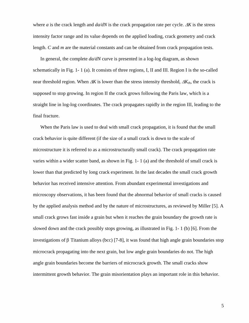
In general, the complete da/dN curve is presented in a log-log diagram, as shown
schematically in Fig. 1- 1 (a). It consists of three regions, I, II and III. Region I is the so-called
near threshold region. When ∆K is lower than the stress intensity threshold, ∆Kth, the crack is
supposed to stop growing. In region II the crack grows following the Paris law, which is a
straight line in log-log coordinates. The crack propagates rapidly in the region III, leading to the
final fracture.
When the Paris law is used to deal with small crack propagation, it is found that the small
crack behavior is quite different (if the size of a small crack is down to the scale of
microstructure it is referred to as a microstructurally small crack). The crack propagation rate
varies within a wider scatter band, as shown in Fig. 1- 1 (a) and the threshold of small crack is
lower than that predicted by long crack experiment. In the last decades the small crack growth
behavior has received intensive attention. From abundant experimental investigations and
microscopy observations, it has been found that the abnormal behavior of small cracks is caused
by the applied analysis method and by the nature of microstructures, as reviewed by Miller [5]. A
small crack grows fast inside a grain but when it reaches the grain boundary the growth rate is
slowed down and the crack possibly stops growing, as illustrated in Fig. 1- 1 (b) [6]. From the
investigations of β Titanium alloys (bcc) [7-8], it was found that high angle grain boundaries stop
microcrack propagating into the next grain, but low angle grain boundaries do not. The high
angle grain boundaries become the barriers of microcrack growth. The small cracks show
intermittent growth behavior. The grain misorientation plays an important role in this behavior.
5

(a) (b)
Fig. 1- 1 Schemes of (a) crack propagation curve and (b) small crack growth behaviour
Small crack
Long crack
∆Kth
II III I
da/d
N
da/d
N
a ∆K
1.1.2 Fatigue Test-Strain Cycling and Stress Cycling
The first study on fatigue test was made by Albert in 1829 with a device which applied cyclic
loadings to a chain made of iron in order to find the number of cycles until fracture [1]. These
kinds of experiments can be referred to as total-life fatigue tests and are still carried out
nowadays for the study of the fatigue behavior of engineering components. With the
development of theories about fatigue and fracture, more advanced test machines have been
invented for more comprehensive fatigue tests. A wide spectrum of materials has been tested
with different loading and environment conditions. The experimental methods most commonly
used for investigation of the essential fatigue behavior of materials are rotary bending and
tension-compression (push-pull) fatigue tests.
With respect to loading conditions, the push-pull test can be divided into two types, stress
cycling and strain cycling fatigue tests [9]. The data obtained from both of these tests are used
for the fatigue resistant design of engineering structures. The so called stress cycling experiment,
which is also referred to as high-cycle fatigue test, is analogous to the situation where the stress
6
level in components is much lower than yield stress. The strain cycling fatigue experiment,
which is referred to as the low-cycle fatigue test, is more interesting for the purpose of fatigue
life evaluation because the stress state in the specimen is more similar to that near the root of
notches in the component, where the local stress level can be close to or even higher than the
yield strength and the plastic deformation may occur. For both stress and strain cycling tests, the
influence factors on fatigue life are: loading amplitude, loading ratio R (minimum to maximum
amplitude), loading frequency f (or loading rate), temperature and environment media. The
symmetrical push-pull loading, i.e. R is -1, is often applied. The fatigue behavior of material can
differ with loading rate but when the loading rate is lower than a critical value (depending on the
material), the fatigue behavior of the material is almost rate-independent.
The fatigue behavior tested by stress cycling is different from that by strain cycling. In strain
cycling fatigue, the strain amplitude is constant during the experiment. For most aluminum alloys
and some types of steels, cyclic hardening behavior, i.e. the stress level increases with fatigue
cycles, is often observed. If the stress level varies in the other way around, i.e. the stress level
decreases with cycles, as observed in some hardened or strengthened materials, e.g. martensitic
steel, cyclic softening happens [9-11].
1.1.3 Damage Accumulation during Multiple Crack Initiation
Multiple crack initiation has received significant attention recently. The availability of
multiple sites for crack initiation makes it a common feature in many kinds of material failures,
such as in the conventional fatigue for steels [12-14], Ni-based superalloy [15], α-irons [16-17]
and cast aluminum alloy [18], as well as in thermal fatigue [19] and in the fatigue of welding
[20]. From these studies, the following common characteristics are found:
- The most dominant cracks were observed in larger grains.
7
- The crack initiation mechanism varies with temperature and chemical composition. For
example in [16], at low temperature the initiation mechanism was intergranular initiation
and at room temperature most cracks initiated were transgranular cracks. In [14], the crack
growth in the ferrite phase was stopped by the pearlite phase and ferrite grain boundaries.
- There are several types of cracks, one-segment cracks (i.e. the microcracks with no kinks)
and multi-segment kinked cracks, observed on the surface. The process of damage
accumulation is the combination of crack initiation, growth and coalescence.
- In order to evaluate fatigue damage accumulation quantitatively, the crack density, i.e. the
number of microcracks per unit surface area of the specimen, is introduced. The crack
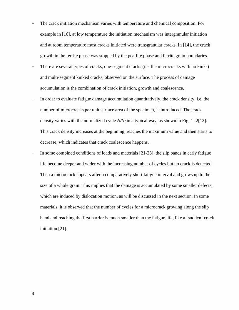
density varies with the normalized cycle N/Nf in a typical way, as shown in Fig. 1- 2[12].
This crack density increases at the beginning, reaches the maximum value and then starts to
decrease, which indicates that crack coalescence happens.
- In some combined conditions of loads and materials [21-23], the slip bands in early fatigue
life become deeper and wider with the increasing number of cycles but no crack is detected.
Then a microcrack appears after a comparatively short fatigue interval and grows up to the
size of a whole grain. This implies that the damage is accumulated by some smaller defects,
which are induced by dislocation motion, as will be discussed in the next section. In some
materials, it is observed that the number of cycles for a microcrack growing along the slip
band and reaching the first barrier is much smaller than the fatigue life, like a ‘sudden’ crack
initiation [21].
8
Cra
ck d
ensi
ty
N/Nf
Fig. 1- 2 A schematic drawing of the crack density varying with the normalized number of fatigue cycles
1.2 Mechanism of Crack Initiation
Fatigue cracks are found initiating not only at the sites of inclusions, scratches or some other
defects, but also from the well-polished surface of fine and uniform materials under fatigue
loading, according to laboratory investigations. An early research about fatigue damage on an
apparently defect-free surface was performed by Ewing and Humfrey [24]. In the experiments
with Swedish iron (ferrite) subjected to rotary bending fatigue they found some slip bands on the
surface. The slip was particularly intense along the slip bands. These slip bands were named
‘persistent slip bands’ (PSB) and crack initiated from these PSBs. In this section the mechanisms
of PSB formation and crack initiation along PSBs will be described.
1.2.1 Mechanism of PSB Formation
Since the phenomenon of persistent slip band (PSB) was discovered, many researches have
been devoted to the investigation of how the PSB forms and the relation of PSB formation with
fatigue loading and fatigue life. From the study on the behavior of single crystal fatigue (mostly
fcc metals, such as copper and nickel), it has been found that the PSB formation is the result of
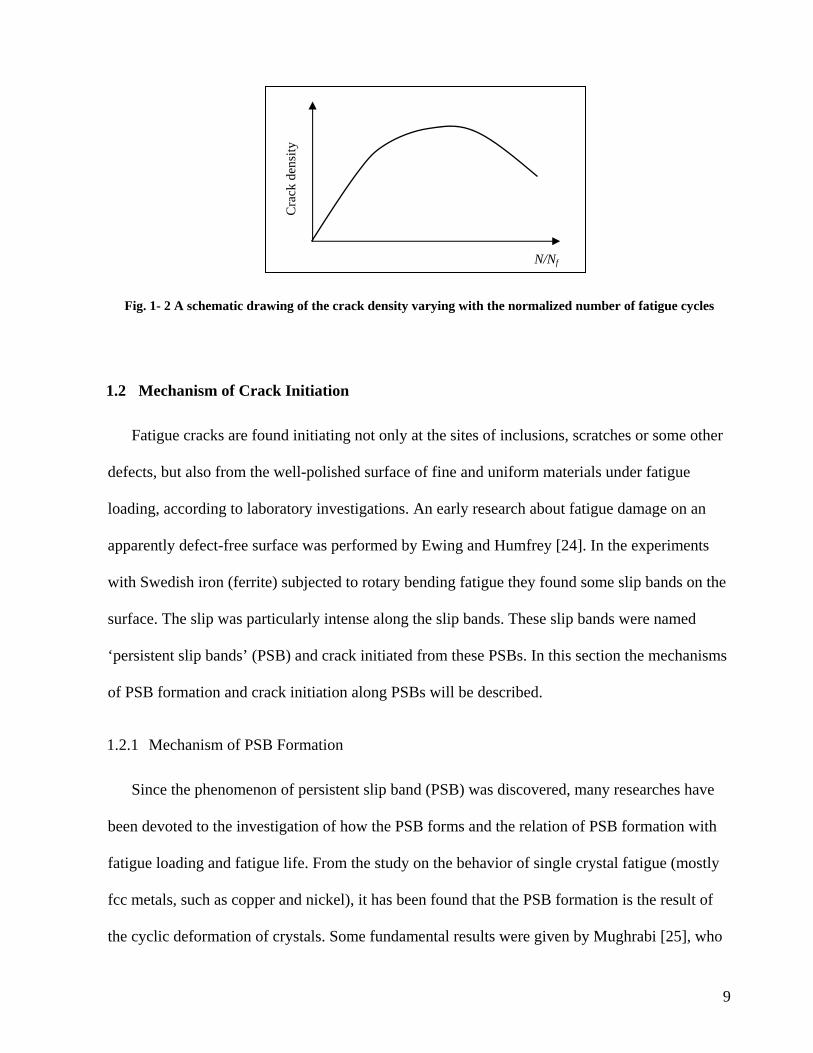
the cyclic deformation of crystals. Some fundamental results were given by Mughrabi [25], who
9
studied the cyclic deformation behavior of a pure copper single crystal under fully reversed
cyclic loading. It was found that the PSB is related to the amplitude of resolved plastic shear
strain γpl. Fig. 1- 3 shows the peak value curve of cyclic resolved shear stress τs versus γpl for Cu
single crystal oriented for single slip. The τs-γpl curve shows different characteristics in three
regions, A, B and C. When the applied plastic shear strain γpl is lower than γpl,AB (in region A),
the shear stress τs increases with γpl and approaches to a critical shear stress τ*s, saturation stress,
from which a plateau of the curve starts. In region A, fine slip markings can be observed but
there is no progressively accumulated damage. The persistent slip bands form at the beginning of
region B, from where the plastic shear strain amplitude is larger than γpl,AB. The volume portion
of PSB increases with the amplitude of γpl proportionally [26] in region B and PSBs will cover
the whole grain when γpl approaches to γpl,BC. A similar mode of behavior has been found later in
some other fcc and bcc single crystals and also in some polycrystalline materials [1].
In fcc single crystal oriented for multiple-slip, however, the hardening behavior is somewhat
different. From the research of Gong et al. [27] it was found that the plateau of shear stress-
plastic shear strain curve (range B in Fig. 1- 3) disappeared for Cu single crystal oriented for
multiple-slip and the well-defined PSBs are not commonly found. This implies that the PSBs
form dominantly in the single slip plane.
Fig. 1- 3 Schematic of hear stress-plastic shear strain curve of fcc single crystal
sτ
*sτ
ABpl ,γ plγBCpl ,γ
A B C
10
There are fewer studies on the mechanism of PSB formation in bcc materials, although the
PSB was first discovered in a low carbon α−iron. The fatigue behavior of pure bcc materials is
very different from that of pure fcc materials. The strain hardening curves of a pure bcc single
crystal show very strong temperature, strain rate and impurity dependence [9]. If the temperature
is higher than a transition temperature Tk or the strain rate is low enough, or when impurity
elements are added, even if the amount is very small, the cyclic deformation behavior of bcc
changes significantly. Under these conditions, the cyclic deformation in bcc material can be quite
similar to that of fcc material. In the research of Sommer [16] on the low cycle fatigue behavior
of α-iron, with the added carbon content of only 74 wt ppm, the PSBs were observed, where the
experimental temperature was above 343K and the strain rate was slower than 1×10⁻⁴ /s. The
persistent slip bands were observed on the surfaces of a low carbon steel [28] and in the ferrite
phase of a steel [29] as well.
The PSB is a group of slip planes usually spreading in the whole grain size. The cyclic
loading induced surface roughness, the extrusions and intrusions which were identified by
scanning electron microscope, are located at the sites of PSBs. By advanced microscopic
techniques, such as the atomic force microscope (AFM), the microstructure of persistent slip
bands can be well-observed [30-31]. The profile of extrusions is approximately triangular and
they grow during fatigue life in the direction of the active slip. Microhardness measurement on
the PSB revealed that the PSB is softer than the matrix, therefore the material deformation is
mostly carried by PSBs.
1.2.2 Mechanism of Crack Initiation from PSB
The crack initiation in defect-free materials is found mostly taking place at PSBs. The
locations of crack nucleation are reported at the PSB-matrix interface [32], at the root of
intrusions [33] and extrusions [34]. The surface roughness is the result of irreversible dislocation
11
motion instigated by fatigue load cycles. From the observation of transmission electron
microscopy (reviewed by Suresh[1]) it is revealed that a dipole consisting of edge dislocations of
opposite signs will annihilate to form a vacancy if the space between them is smaller than a
critical value. The annihilation of dipoles is responsible for the extrusions and the interstitial-type
dipoles are responsible for intrusions.
The crack nucleation mechanism proposed by Essmann et al. [35] gives a detailed
microscopic description of the irreversible glide in PSBs based on the analysis of dislocation
movement. The hypothesis is that the annihilation of vacancy-type dipoles is the dominant point-
defect generation process and that the annihilation of dislocations within slip bands is the origin
of irreversibility. This irreversible slip can happen when a screw dislocation glides along
different paths forwards and backwards and consequently the PSBs are formed by the
irreversible slip. The extrusion is the PSBs emerging on the surface. The cracks nucleate at the
intersection of the PSBs and surface.
The crack initiation mechanism proposed by Lin and Ito [36] and Tanaka and Mura [37] is
also based on the formation of intrusions and extrusions and the irreversibility of dislocation
motion. But here, the dislocation motion is described on the two adjacent parallel slip planes.
The proposed mechanism has the background of experiment observations where it was found
that the slip plane during the tensile loading and the one during compressive loading were closely
spaced but, in fact, distinct from each other [1].
1.2.3 Mechanism of Crack Initiation at Inclusions
There are two typical damage modes regarding the crack initiation at inclusions: (i) the
debonding of the inclusion from the matrix when the adhesion between inclusion and matrix is
weak [38] and (ii) the breaking of the inclusion when the inclusion strength is lower than the
matrix [39]. Matrix microcracks nucleate at the sites of the interfaces between the inclusion and
12
matrix. Crack initiating near inclusions can also be of the slip band type [38]. The size of
inclusion is found to be a critical factor. For example, the work of Laz and Hillberry [39] on
2024-T3 aluminum alloy indicates that the size of cracked inclusions is larger than 5µm. Another
phenomenon often observed in the material containing inclusions is the subsurface crack
initiation when the inclusion size is large. Very small inclusions (<1 µm, for example) can
suppress crack initiation through slip homogenization [9].
1.3 Models of Crack Initiation
1.3.1 Conventional Models
The early prediction models for crack initiation are based on the low-cycle fatigue
experiment and the Manson-Coffin equation. From the fatigue experiment, the relation of
loading level (stress range ∆σ in stress cycling and strain range ∆ε or plastic strain range ∆εp in
strain or plastic strain cycling) and the number of cycles to specimen failure Nf can be obtained.
The general form of the relation, found by Coffin and Manson e.g. for low-cycle fatigue, is in the
form of a power function as the following equation,
cff
p N )2(2
'εε
=∆
(1-2)
where 2Nf is the number of load reversals to failure, the fatigue ductility coefficient and c the
fatigue ductility exponent. and c are material parameters. Equation (1-2) is still widely used
nowadays. However, the microstructural influence cannot be described by Eq. (1-2). One model
proposed by Cheng and Laird [40] has a similar form:
'fε
'fε
'
2CN f
p =∆ αγ
(1-3)
13
where ∆γp is the plastic shear strain range, C’ and α are material constants. Eq. (1-3) was
developed on the basis of PSB formation but it does not provide any explicit microstructural
parameter.
1.3.2 Microstructure-Based Models
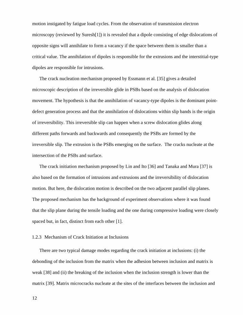
The life prediction model proposed by Tanaka and Mura [37] for the crack initiation from
slip bands yields the relations between the number of cycles to crack initiation and material
parameters. This model is based on the assumption that irreversible dislocation pile-ups cause
crack initiation. In order to incorporate slip irreversibility, the deformation within slip bands is
modeled by two closely adjacent layers of dislocation pile-ups. The dislocations in each layer
have different signs, as shown in Fig. 1- 4. It is assumed that the motion of dislocations formed
by previous forward loading in layer I are irreversible and that the reverse plastic flow is taken
up by the motion of dislocations with the opposite sign on layer II. The positive back stress
induced by the positive dislocation pile-ups in layer I facilitates the pile-up of the negative
dislocations in layer II. This process continues with loading cycles. The progress of dislocation
accumulation is calculated by using the theory of continuously distributed dislocations. The
strain energy of dislocation is accumulated to the same extent in each forward and reverse
loading. When the accumulated energy reaches the amount of fracture energy, a crack initiates.
According to the Tanaka-Mura model, the quantitative equation to estimate the crack
initiation life Nc for the stage I crack is derived as:
2)2()1(8
kdGW
N sc −∆−
=τνπ
(1-4)
where G is the shear modulus and ν the Poisson’s ratio, Ws is the specific fracture energy for a
unit area consisting of the surface energy and the plastic fracture work. ∆τ is the resolved shear
stress range, which is the stress range from the minimum shear stress to the maximum shear
14
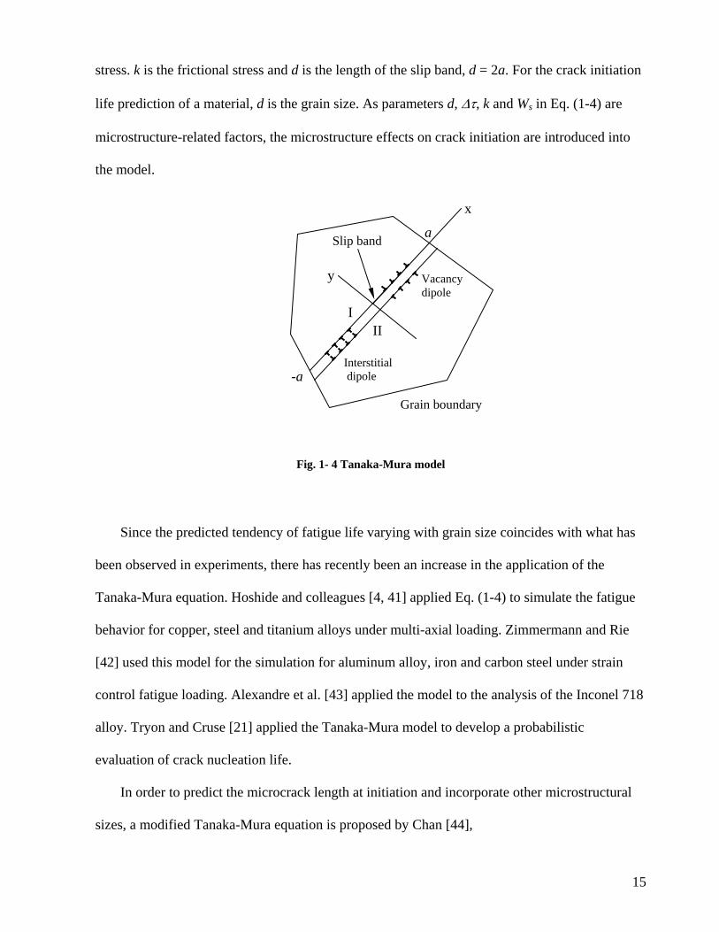
stress. k is the frictional stress and d is the length of the slip band, d = 2a. For the crack initiation
life prediction of a material, d is the grain size. As parameters d, ∆τ, k and Ws in Eq. (1-4) are
microstructure-related factors, the microstructure effects on crack initiation are introduced into
the model.
Fig. 1- 4 Tanaka-Mura model
Since the predicted tendency of fatigue life varying with grain size coincides with what has
been observed in experiments, there has recently been an increase in the application of the
Tanaka-Mura equation. Hoshide and colleagues [4, 41] applied Eq. (1-4) to simulate the fatigue
behavior for copper, steel and titanium alloys under multi-axial loading. Zimmermann and Rie
[42] used this model for the simulation for aluminum alloy, iron and carbon steel under strain
control fatigue loading. Alexandre et al. [43] applied the model to the analysis of the Inconel 718
alloy. Tryon and Cruse [21] applied the Tanaka-Mura model to develop a probabilistic
evaluation of crack nucleation life.
In order to predict the microcrack length at initiation and incorporate other microstructural
sizes, a modified Tanaka-Mura equation is proposed by Chan [44],
-a
Slip band
Interstitial dipole
Vacancy dipole
I II
a
y
x
Grain boundary
15
)()()2)(1(
8 2
2
2
dc
dh
kGN ⋅
−∆−=
τνλπ (1- 5)
where three more additional variables are introduced: c is half of the length or the depth of an
incipient crack (the size can be a part of the slip band), h is the width of the slip band and
parameter λ is a constant, λ = 0.005. This model is developed on the assumption that the
dislocation dipoles contribute to the crack formation and the criterion of crack formation is
seq dW γ2=
where γs is the surface energy and Weq is the strain energy stored in the dislocation dipoles of a
single slip band. For the convenience of description, Eq. (1-5) is rewritten as following:
Gdhc
kdGNi ⋅⋅⋅
−∆−= 2
2)(
)2()1(8
λτνπ (1-6)
The left term in the right-hand side of Eq. (1-6) is similar to the Tanaka-Mura equation (see Eq.
(1-4)) but the specific fracture energy Ws is replaced by
GdhcW ss
2)(⋅==λ
γ (1-7)
In Eq.(1-7), the fracture energy Ws is considered to be only composed of surface energy γs.
The above two models include the most influencing microstructural parameters for the life
prediction of microcrack initiation. Most of the parameters can be determined by standard
experiments and only a few are needed to be defined by additional investigation.
The observation of crack nucleation on the surface by means of an atomic force microscope
(AFM) can give more detailed information because of its high resolution. Based on this new
technology, Harvey et al. [45] proposed a model to predict fatigue crack initiation life by means
of these microscopic parameters:
epys
thi hEf
KN
εσ ∆∆
=4
2
(1- 8)
16
where ∆Kth is the long crack propagation threshold, σys is the yield strength of material, E is the
Young’s modulus and ∆εp is the plastic strain range. The value of these parameters can be
obtained with standard tests. he is the slip spacing and f is the fraction of plastic strain range of
applied loading, which is related to the slip height δ. δ and he can be measured from the records
of AFM photographs on the surface. It is supposed that a crack will initiate when the cumulative
slip height reaches the threshold of crack-opening displacement.
1.3.3 Models Based on Probability
Due to the pronounced influence of the microstructure, crack initiation is a stochastic process
and is dealt with by initiation probability in some models [21, 47-51]. Some of them are derived
from empirical equations based on the investigation of specimen surfaces [46-47] and the
number of cracks is the random variable. Some other models combine the microstructure-based
model with the stochastic model, such as the model proposed by Tryon and Cruse [21]. In their
model the Tanaka-Mura model is employed for the evaluation of the number of cycles to crack
initiation to a grain size. The model applied by Morris et al. [48] is to simulate crack initiation
from inclusions. In this case the crack initiation life is a function of microstructure parameters
[49], such as the inclusion size, the distance of the inclusion to the grain boundary and the
effective stress. In the statistical model of Ihara et al. [50] the energy stored in the material of
each cycle was the basic random variable. The criterion for crack initiation is the formation of a
PSB when the accumulated energy is higher than a critical value. A stochastic model, recently
developed by Meyer and Brückner-Foit [51], is focused on the influence of microstructure
parameters on low-cycle fatigue life using a planar random cell structure. In this model the crack
initiation probability depends not only on the strain amplitude, but also on the microstructure
variables, such as individual grain size and orientation.
17
1.4 Modeling of Polycrystal Materials
1.4.1 Representative Volume Element
In order to establish the macroscopic relation of mechanical and physical properties to the
real material microconstituents and microstructures, the concept of representative volume
element (RVE) is introduced [52]. An RVE is a material volume which is statistically
representative of the infinitesimal material point and its neighborhood. The RVE can have many
kinds of micro-elements, such as grains separated by grain boundaries, inclusions, voids,
microcracks and other similar defects. It provides a mesoscopic analysis tool which links the
macroscopic homogenous material and its inhomogeneous microstructure.
The size of an RVE is macroscopically infinitesimal compared to the scale of the bulk
material and its boundary conditions, so that the local stress state can be accurately represented.
On the other hand, the RVE is microscopically large enough to represent the real material
microconstituents and microstructures, and the micro-damage evolving process. As shown in
Fig. 1- 5, L is the scale of bulk material, H is the scale of boundary conditions on bulk, D is the
scale of the RVE and d the microstructure scale inside the RVE. The magnitudes of L, H, D and
d satisfy the relations of D<<L, d<<D and D<<H.
The suitable size of an RVE depends on which material and what property will be studied.
Lemaitre [53] suggested the RVE size to be 0.1×0.1×0.1 mm3 for metals. From the finite
element numerical analyses carried out by Ren and Zheng [54], it was found that the error of
material moduli between the macroscopic material constants and the results obtained from a two-
dimensional RVE, which was 20 times larger than grain size, was 5% for several polycrystalline
materials. It was concluded that the absolute size of an RVE was not so critical. The important
geometric dimensions were the relative scales of the three constituents, L(H), D and d.
18
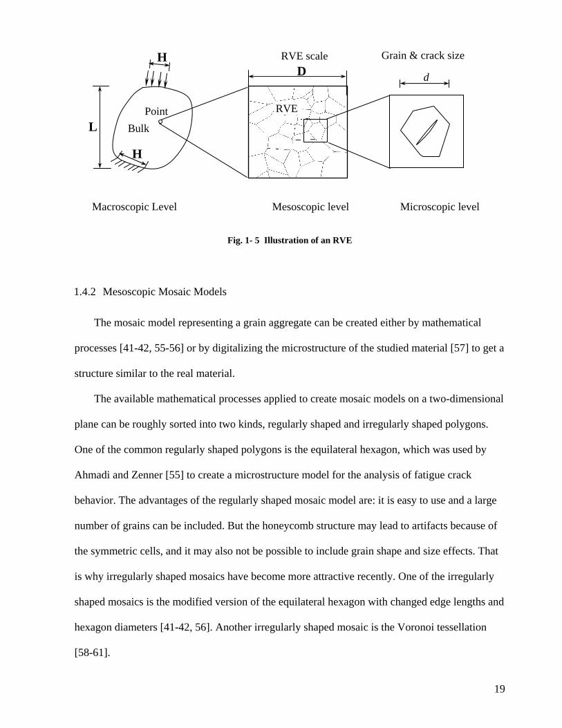
Fig. 1- 5 Illustration of an RVE
RVE
Mesoscopic level Microscopic level
Bulk Point
H
H
L
Grain & crack size
d DRVE scale
Macroscopic Level
1.4.2 Mesoscopic Mosaic Models
The mosaic model representing a grain aggregate can be created either by mathematical
processes [41-42, 55-56] or by digitalizing the microstructure of the studied material [57] to get a
structure similar to the real material.
The available mathematical processes applied to create mosaic models on a two-dimensional
plane can be roughly sorted into two kinds, regularly shaped and irregularly shaped polygons.
One of the common regularly shaped polygons is the equilateral hexagon, which was used by
Ahmadi and Zenner [55] to create a microstructure model for the analysis of fatigue crack
behavior. The advantages of the regularly shaped mosaic model are: it is easy to use and a large
number of grains can be included. But the honeycomb structure may lead to artifacts because of
the symmetric cells, and it may also not be possible to include grain shape and size effects. That
is why irregularly shaped mosaics have become more attractive recently. One of the irregularly
shaped mosaics is the modified version of the equilateral hexagon with changed edge lengths and
hexagon diameters [41-42, 56]. Another irregularly shaped mosaic is the Voronoi tessellation
[58-61].
19
The Voronoi tessellation is generated by the Poisson point process which randomly divides
the space into regions and these regions completely fill up the space without overlapping. These
regions are convex polygons with various numbers of edges on a two-dimensional plane or
polyhedral cells with planar faces in three-dimensional space. These polyhedral or polygonal
cells are generated from randomly distributed nuclei and the shared edges or faces of two cells
are located in the middle distance of the nuclei from which they are formed. From the physical
point of view this is very similar to the polycrystalline microstructures of most metals and
ceramics (Kumar et al. [62]) and it finds applications originally in material science. The mosaic
model created by Voronoi tessellation allows more microstructure parameters to be introduced
than in the regularly shaped mosaic. It is used more often nowadays in the stress analyses for the
non-damaged [58-59] or damaged [60-61] polycrystalline materials. But the Voronoi tessellation
is not exactly the same as a real grain structure. The spatial topology is, to a higher or lesser
degree, different from a real grain aggregate. Additionally, the shape of grains with rounded
vertex in materials cannot be simulated by Voronoi cell.
20
CHAPTER 2 EXPERIMENTAL DATA AND STATISTICAL ANALYSIS
The studied material, a Japanese stainless steel F82H, is a kind of reduced activation steel
for structural application in fusion systems. The work concerning experiments and statistics was
done in a previous project and the data obtained thereby were stored in a database [63]. The
information about material properties, experimental data and statistical analysis for the crack
initiation presented in this chapter, is quoted from this database in order to give the background
of the simulation. This chapter consists of six sections. In Section 2.1 the material microstructure
and the mechanical properties are introduced. The experimental procedure of low cycle fatigue is
described in Section 2.2 and the fatigue data obtained from experiment are presented in Section
2.3. In Section 2.4 some important observations and statistical results based on the research of
Bertsch [63] and Meyer [64] are quoted to clarify the damage accumulation process and the
fatigue failure mechanism of the material. In Section 2.5 a short summary of the characteristics of
crack initiation is given. The scatter of experimental data is discussed in Section 2.6.
2.1 Material
The chemical composition of F82H steel is shown in Table 2-1. The content of Chromium-
equivalent is 10.139% and the content of Nickel-equivalent is 2.979%, which are determined by
Eq. (2-1). From the Schaeffler-Diagram of Ni-equivalent to Cr-equivalent, the composition of
F82H is in the martensite region but very close to the martensite-ferrite region.
21
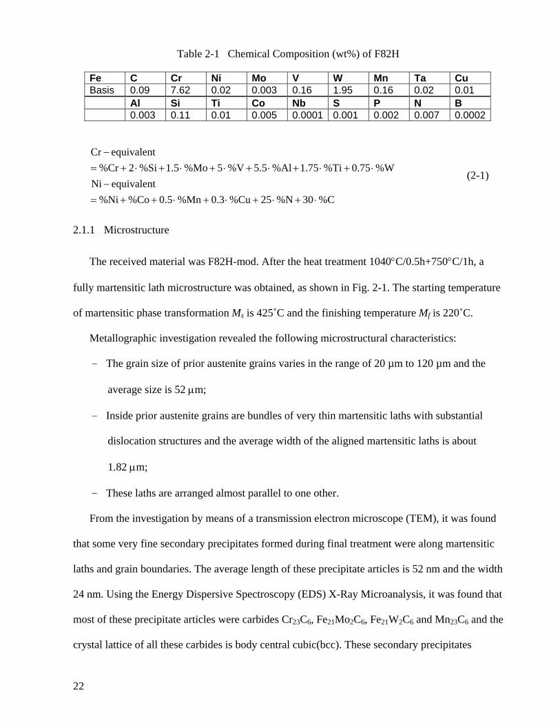
Table 2-1 Chemical Composition (wt%) of F82H
Fe C Cr Ni Mo V W Mn Ta Cu Basis 0.09 7.62 0.02 0.003 0.16 1.95 0.16 0.02 0.01 Al Si Ti Co Nb S P N B 0.003 0.11 0.01 0.005 0.0001 0.001 0.002 0.007 0.0002
%C30%N25%Cu0.3%Mn0.5%Co%NiequivalentNi
%W0.75%Ti1.75%Al5.5%V5%Mo1.5%Si2%CrequivalentCr
⋅+⋅+⋅+⋅++=−
⋅+⋅+⋅+⋅+⋅+⋅+=−
(2-1)
2.1.1 Microstructure
The received material was F82H-mod. After the heat treatment 1040°C/0.5h+750°C/1h, a
fully martensitic lath microstructure was obtained, as shown in Fig. 2-1. The starting temperature
of martensitic phase transformation Ms is 425˚C and the finishing temperature Mf is 220˚C.
Metallographic investigation revealed the following microstructural characteristics:
- The grain size of prior austenite grains varies in the range of 20 µm to 120 µm and the
average size is 52 µm;
- Inside prior austenite grains are bundles of very thin martensitic laths with substantial
dislocation structures and the average width of the aligned martensitic laths is about
1.82 µm;
- These laths are arranged almost parallel to one other.
From the investigation by means of a transmission electron microscope (TEM), it was found
that some very fine secondary precipitates formed during final treatment were along martensitic
laths and grain boundaries. The average length of these precipitate articles is 52 nm and the width
24 nm. Using the Energy Dispersive Spectroscopy (EDS) X-Ray Microanalysis, it was found that
most of these precipitate articles were carbides Cr23C6, Fe21Mo2C6, Fe21W2C6 and Mn23C6 and the
crystal lattice of all these carbides is body central cubic(bcc). These secondary precipitates
22
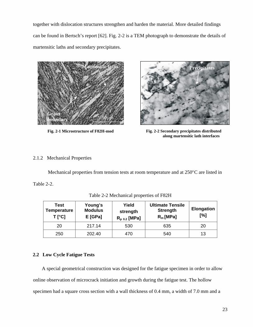
together with dislocation structures strengthen and harden the material. More detailed findings
can be found in Bertsch’s report [62]. Fig. 2-2 is a TEM photograph to demonstrate the details of
martensitic laths and secondary precipitates.
Precipitates
50µmGrain boundary
Martensitic laths
Fig. 2-2 Secondary precipitates distributed along martensitic lath interfaces
Fig. 2-1 Microstructure of F82H-mod
2.1.2 Mechanical Properties
Mechanical properties from tension tests at room temperature and at 250°C are listed in
Table 2-2.
Table 2-2 Mechanical properties of F82H
Test Temperature
T [°C]
Young’s Modulus E [GPa]
Yield strength
Rp 0.2 [MPa]
Ultimate Tensile Strength Rm [MPa]
Elongation[%]
20 217.14 530 635 20
250 202.40 470 540 13
2.2 Low Cycle Fatigue Tests
A special geometrical construction was designed for the fatigue specimen in order to allow
online observation of microcrack initiation and growth during the fatigue test. The hollow
specimen had a square cross section with a wall thickness of 0.4 mm, a width of 7.0 mm and a
23
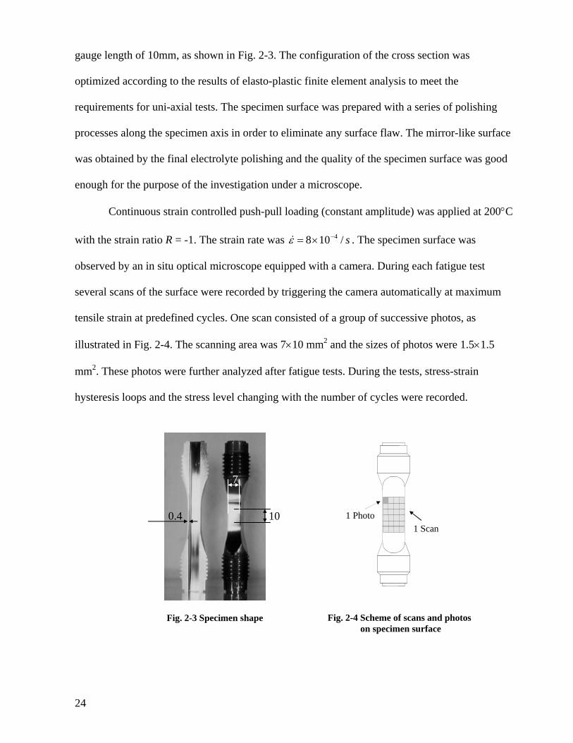
gauge length of 10mm, as shown in Fig. 2-3. The configuration of the cross section was
optimized according to the results of elasto-plastic finite element analysis to meet the
requirements for uni-axial tests. The specimen surface was prepared with a series of polishing
processes along the specimen axis in order to eliminate any surface flaw. The mirror-like surface
was obtained by the final electrolyte polishing and the quality of the specimen surface was good
enough for the purpose of the investigation under a microscope.
Continuous strain controlled push-pull loading (constant amplitude) was applied at 200°C
with the strain ratio R = -1. The strain rate was . The specimen surface was
observed by an in situ optical microscope equipped with a camera. During each fatigue test
several scans of the surface were recorded by triggering the camera automatically at maximum
tensile strain at predefined cycles. One scan consisted of a group of successive photos, as
illustrated in Fig. 2-4. The scanning area was 7×10 mm2 and the sizes of photos were 1.5×1.5
mm2. These photos were further analyzed after fatigue tests. During the tests, stress-strain
hysteresis loops and the stress level changing with the number of cycles were recorded.
s/108 4−×=ε&
0.4
7
10 1 Photo1 Scan
Fig. 2-4 Scheme of scans and photos on specimen surface
Fig. 2-3 Specimen shape
24
2.3 Experiment Results
2.3.1 Fatigue Life
Table 2-3 lists all the experimental data of fatigue life Nf varying with strain range ∆ε,
where ∆ε is the total strain range of a specimen and equals εmax-εmin.
2.3.2 Elasto-Plastic Behavior Obtained from Experiment Data
The total strain amplitude ∆ε/2 is written as the sum of the elastic strain amplitude ∆εe/2 and
the plastic strain amplitude ∆εp/2:
The elastic strain amplitude ∆εe/2 and plastic strain amplitude ∆εp/2 are calculated from
experimental data, ∆σ/2 and ∆ε/2, and are listed in Table 2-4.
2/2/2/ pe εεε ∆+∆=∆
Table 2-3 Fatigue data obtained from experiment
Specimen ID ∆ε [%] Cycles to failure
V190 0.90 2700
V201 0.90 2740
V202 0.80 2690
V192 0.76 4600
V193 0.65 6950
V209 0.64 5180
V203 0.60 5940
V214 0.58 6890
V205 0.55 8210
V213 0.50 13170
V197 0.50 16860
V210 0.44 45800
25
Table 2-4 Elastic and plastic strain amplitudes of specimens
Specimen ID
Stress amplitude
∆σ/2 [MPa]
Total strain amplitude
∆ε/2 [%]
Elastic strain amplitude
∆εe/2 [%]
Plastic strain amplitude
∆εp/2 [%]
V201 462.0 0.45 0.2283 0.2207
V202 447.8 0.40 0.2212 0.1780
V192 408.5 0.38 0.2018 0.1775
V193 401.3 0.326 0.1983 0.1272
V209 401.3 0.32 0.1983 0.1212
V203 403.2 0.30 0.1992 0.1004
V214 377.1 0.29 0.1863 0.1033
V205 375.0 0.275 0.1853 0.0893
V197 366.9 0.25 0.1813 0.0684
V213 350.9 0.25 0.1734 0.0763
V210 313.7 0.22 0.1550 0.0647
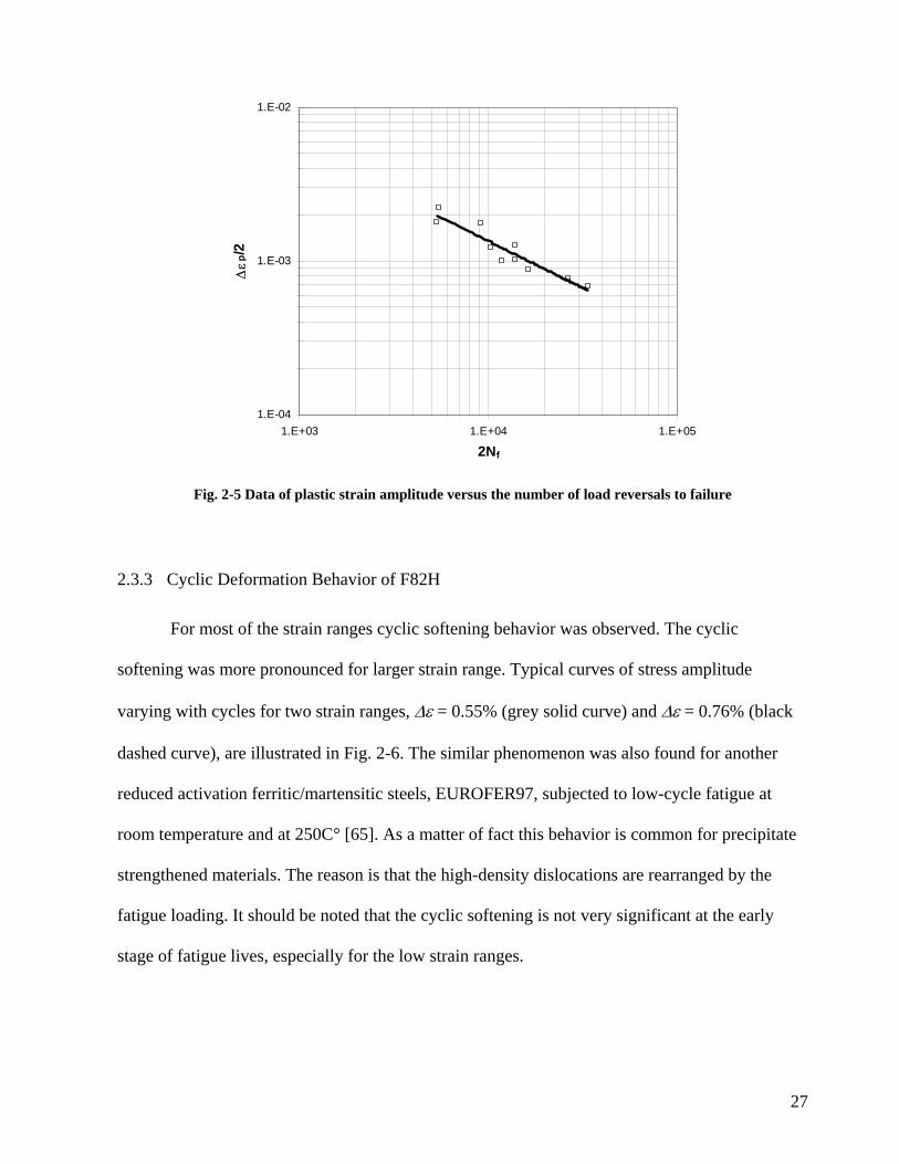
In the log-log plot of Fig. 2-5 the data of plastic strain amplitude ∆εp/2 versus the number
of load reversals to failure 2Nf are presented by open symbols and the derived relation is
presented by the bold line. Based on the experimental data, the Coffin-Manson expression of
∆εp/2 with 2Nf for F82H was obtained,
612.0)2(378.02/ −=∆ fp Nε (2-2)
From Eq. (2-2) the fatigue ductility coefficient 'fε = 0.378 and the fatigue ductility
exponent c = -0.612 are obtained. For most of the metals and alloys tested at room temperature
the fatigue ductility exponent c is in the range of -0.5 and -0.7. The value of c for F82H falls
within this range. This means the present material follows the common low cycle fatigue
behavior of metals.
26
1.E-04
1.E-03
1.E-02
1.E+03 1.E+04 1.E+05
2Nf
∆εp
/2
Fig. 2-5 Data of plastic strain amplitude versus the number of load reversals to failure
2.3.3 Cyclic Deformation Behavior of F82H
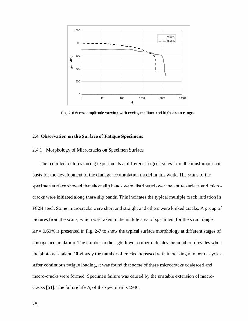
For most of the strain ranges cyclic softening behavior was observed. The cyclic
softening was more pronounced for larger strain range. Typical curves of stress amplitude
varying with cycles for two strain ranges, ∆ε = 0.55% (grey solid curve) and ∆ε = 0.76% (black
dashed curve), are illustrated in Fig. 2-6. The similar phenomenon was also found for another
reduced activation ferritic/martensitic steels, EUROFER97, subjected to low-cycle fatigue at
room temperature and at 250C° [65]. As a matter of fact this behavior is common for precipitate
strengthened materials. The reason is that the high-density dislocations are rearranged by the
fatigue loading. It should be noted that the cyclic softening is not very significant at the early
stage of fatigue lives, especially for the low strain ranges.
27
0
200
400
600
800
1000
1 10 100 1000 10000 100000
N
∆σ
[M
Pa]
0.55%0.76%
Fig. 2-6 Stress amplitude varying with cycles, medium and high strain ranges
2.4 Observation on the Surface of Fatigue Specimens
2.4.1 Morphology of Microcracks on Specimen Surface
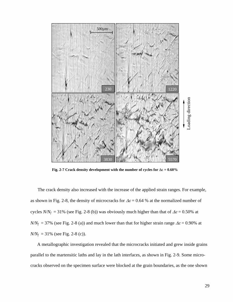
The recorded pictures during experiments at different fatigue cycles form the most important
basis for the development of the damage accumulation model in this work. The scans of the
specimen surface showed that short slip bands were distributed over the entire surface and micro-
cracks were initiated along these slip bands. This indicates the typical multiple crack initiation in
F82H steel. Some microcracks were short and straight and others were kinked cracks. A group of
pictures from the scans, which was taken in the middle area of specimen, for the strain range
∆ε = 0.60% is presented in Fig. 2-7 to show the typical surface morphology at different stages of
damage accumulation. The number in the right lower corner indicates the number of cycles when
the photo was taken. Obviously the number of cracks increased with increasing number of cycles.
After continuous fatigue loading, it was found that some of these microcracks coalesced and
macro-cracks were formed. Specimen failure was caused by the unstable extension of macro-
cracks [51]. The failure life Nf of the specimen is 5940.
28
29
Load
ing
dire
ctio
n
1220
3830
500µm
230
5570
Fig. 2-7 Crack density development with the number of cycles for ∆ε = 0.60%
The crack density also increased with the increase of the applied strain ranges. For example,
as shown in Fig. 2-8, the density of microcracks for ∆ε = 0.64 % at the normalized number of
cycles N/Nf = 31% (see Fig. 2-8 (b)) was obviously much higher than that of ∆ε = 0.50% at
N/Nf = 37% (see Fig. 2-8 (a)) and much lower than that for higher strain range ∆ε = 0.90% at
N/Nf = 31% (see Fig. 2-8 (c)).
A metallographic investigation revealed that the microcracks initiated and grew inside grains
parallel to the martensitic laths and lay in the lath interfaces, as shown in Fig. 2-9. Some micro-
cracks observed on the specimen surface were blocked at the grain boundaries, as the one shown
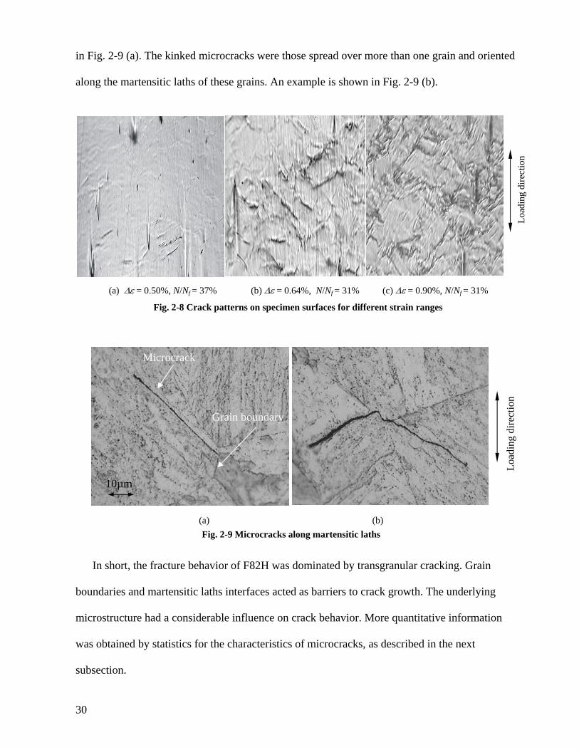
Load
ing
dire
ctio
n
in Fig. 2-9 (a). The kinked microcracks were those spread over more than one grain and oriented
along the martensitic laths of these grains. An example is shown in Fig. 2-9 (b).
(a) ∆ε = 0.50%, N/Nf = 37% (b) ∆ε = 0.64%, N/Nf = 31% (c) ∆ε = 0.90%, N/Nf = 31%
Fig. 2-8 Crack patterns on specimen surfaces for different strain ranges
Grain boundary
Microcrack
10µm
Load
ing
dire
ctio
n
(a) (b) Fig. 2-9 Microcracks along martensitic laths
In short, the fracture behavior of F82H was dominated by transgranular cracking. Grain
boundaries and martensitic laths interfaces acted as barriers to crack growth. The underlying
microstructure had a considerable influence on crack behavior. More quantitative information
was obtained by statistics for the characteristics of microcracks, as described in the next
subsection.
30
2.4.2 Statistics for the Characteristics of Microcracks
The statistics quoted here reveal the crack initiation characteristics in terms of length,
segmentation and orientation.
The microcracks were categorized depending on their geometrical shape as following:
- One-segment cracks are cracks with no kink;
- Two-segment cracks are cracks with one kink;
- Multi-segment cracks are cracks with three or more kinks.
From the statistics it was found that the average size of the one-segment cracks was 79 µm,
somewhat above the prior austenite grain size (52 µm). Therefore, it is reasonable to assume that
one-segment cracks correspond to completely fractured grains, which are often larger in size.
The two-segment cracks, as shown in Fig. 2-9 (b), are formed in such a way that a micro-
crack in one grain overcomes the micro-structural barrier at the grain boundary and grows into
the adjacent grain along the orientation of the martensitic lath of this grain. In the case described
here, very few two-segment cracks were observed, i.e. crack growth is very unlikely.
Cracks with three or more kinks can be formed by crack coalescence or crack growth. The
statistics showed that the average segment length of the crack segments, which was counted on
the segments of all kinds of cracks, was mostly larger than the average grain size for all strain
ranges.
As in-situ scans of the specimen surface are available at pre-defined load cycles, the crack
density, i.e. the number of cracks per unit area, is derived in terms of one-segment cracks and
crack segments. In the diagram of crack density versus the number of cycles for one-segment
cracks and crack segments, as shown in Fig. 2-10, the damage accumulation process is an
evolving procedure with the competition of crack initiation and crack coalescence in different
fatigue stages. The data showed that the number of one-segment cracks and the crack segments
31
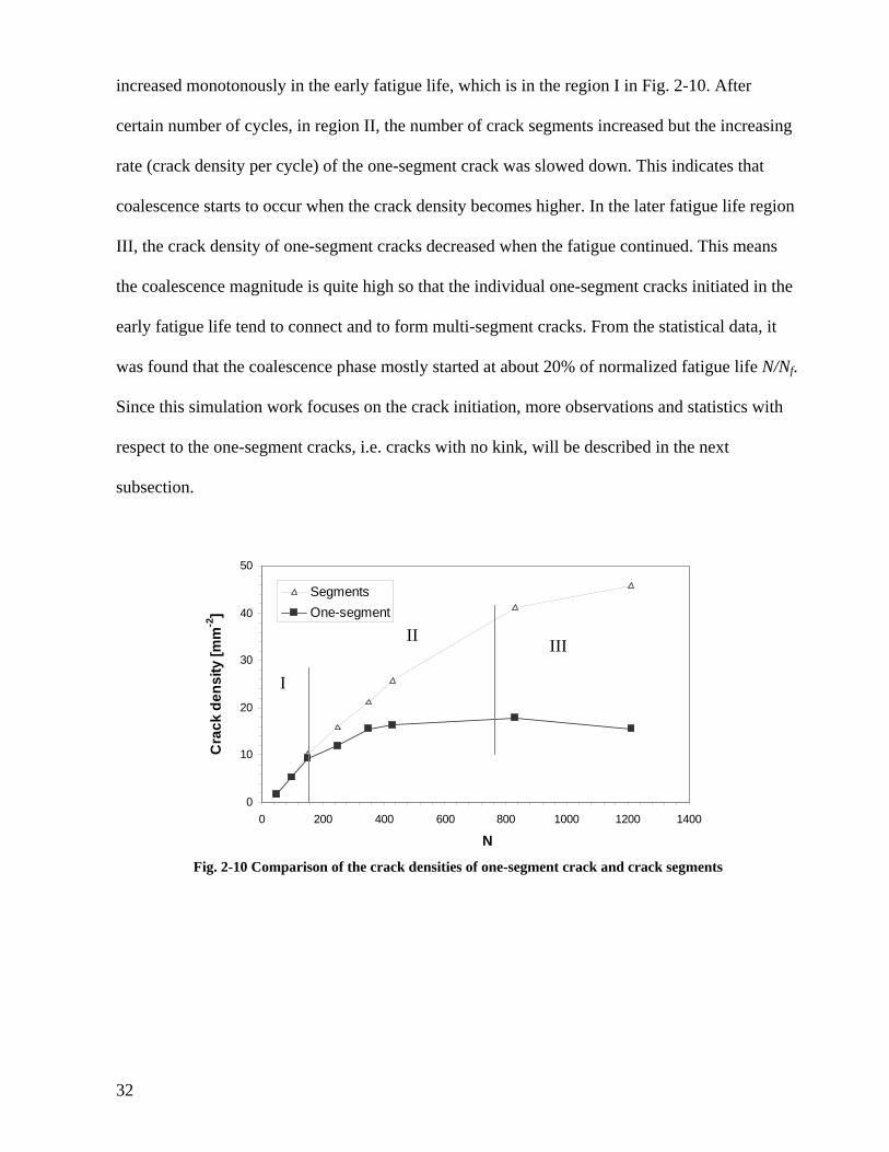
increased monotonously in the early fatigue life, which is in the region I in Fig. 2-10. After
certain number of cycles, in region II, the number of crack segments increased but the increasing
rate (crack density per cycle) of the one-segment crack was slowed down. This indicates that
coalescence starts to occur when the crack density becomes higher. In the later fatigue life region
III, the crack density of one-segment cracks decreased when the fatigue continued. This means
the coalescence magnitude is quite high so that the individual one-segment cracks initiated in the
early fatigue life tend to connect and to form multi-segment cracks. From the statistical data, it
was found that the coalescence phase mostly started at about 20% of normalized fatigue life N/Nf.
Since this simulation work focuses on the crack initiation, more observations and statistics with
respect to the one-segment cracks, i.e. cracks with no kink, will be described in the next
subsection.
0
10
20
30
40
50
0 200 400 600 800 1000 1200 1400
N
Cra
ck d
ensi
ty [m
m-2
]
SegmentsOne-segment
II III
I
Fig. 2-10 Comparison of the crack densities of one-segment crack and crack segments
32
2.4.3 Characteristics of One-Segment Cracks
In the present study, the one-segment crack corresponds to a just initiated microcrack without
kink and is simply referred to as ‘crack’ in the following part of this work.
2.4.3.1 Crack Length
From the statistical data of crack length it was found that, as aforementioned, the average size
of the cracks was longer than the average grain size. This implies that large grains are more likely
to fracture. From the obtained relation for one-segment cracks with the number of cycles, it was
found that some short cracks in the order of the average grain size already started to develop after
a few load cycles. There is no database for the crack extension within one grain, as cracks with
lengths of less than one grain were hard to find in the experiment.
2.4.3.2 Crack Orientation
From the statistical investigation, it was found that the empirical distribution of the
orientation angle of microcracks on the surface was non-uniform with a peak at about 45º to the
loading axis for low and middle strain ranges, although the martensitic lath orientations were
completely uniform. Considering the nature of the crack initiated in slip bands and the fact that
the maximum resolved shear stress occurs on a slip plane orientated in 45°, the crack initiation
mechanism is shear stress driven.
2.4.3.3 Crack Density as the Function of Cycles
As described in the previous section, the damage accumulation process of material F82H is
considered as the combination of two phases, crack initiation phase and crack coalescence phase.
According to the statistics of crack density versus the number of cycles for all the tests under
various strain ranges, the crack density was increasing during the early fatigue life. Statistical
33
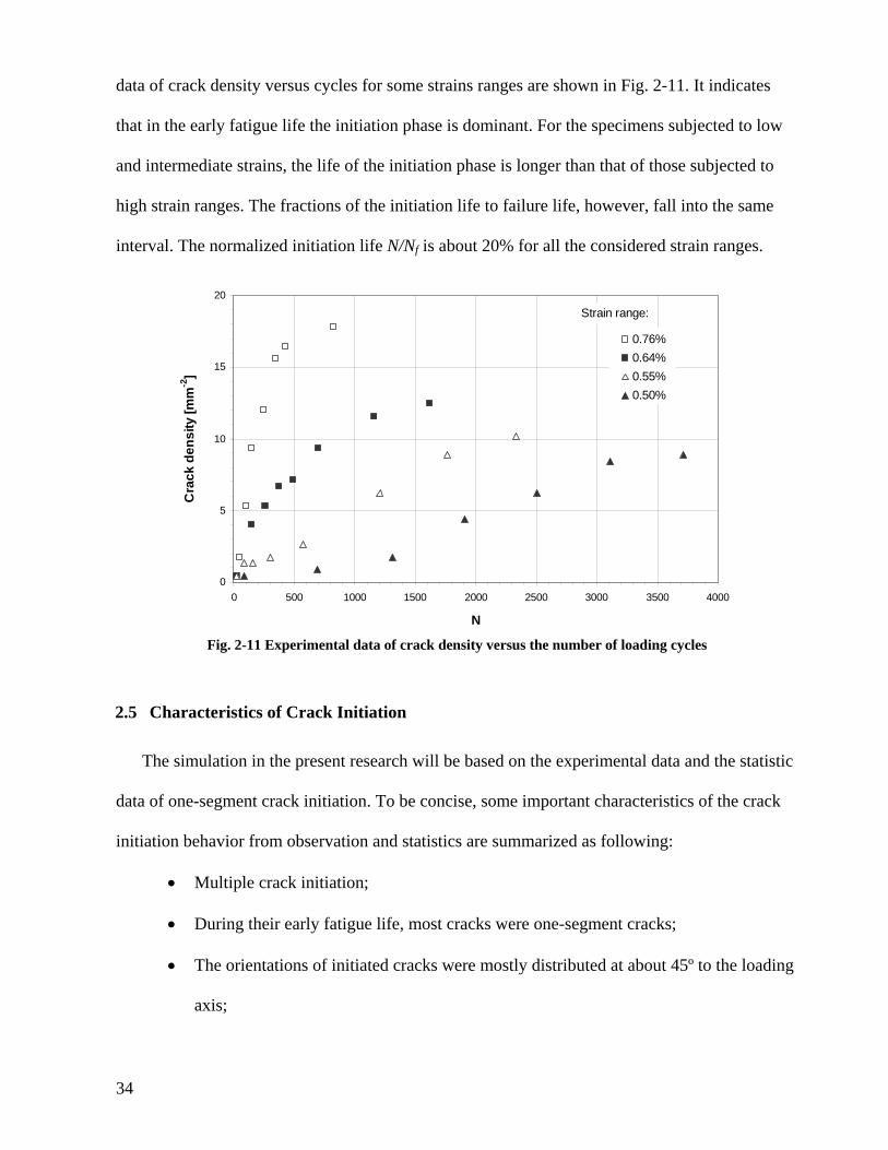
data of crack density versus cycles for some strains ranges are shown in Fig. 2-11. It indicates
that in the early fatigue life the initiation phase is dominant. For the specimens subjected to low
and intermediate strains, the life of the initiation phase is longer than that of those subjected to
high strain ranges. The fractions of the initiation life to failure life, however, fall into the same
interval. The normalized initiation life N/Nf is about 20% for all the considered strain ranges.
Strain range:
0
5
10
15
20
0 500 1000 1500 2000 2500 3000 3500 4000
N
Cra
ck d
ensi
ty [m
m-2
]
0.76%0.64%0.55%0.50%
Fig. 2-11 Experimental data of crack density versus the number of loading cycles
2.5 Characteristics of Crack Initiation
The simulation in the present research will be based on the experimental data and the statistic
data of one-segment crack initiation. To be concise, some important characteristics of the crack
initiation behavior from observation and statistics are summarized as following:
• Multiple crack initiation;
• During their early fatigue life, most cracks were one-segment cracks;
• The orientations of initiated cracks were mostly distributed at about 45º to the loading
axis;
34
• Fatigue cracks were initiated in slip bands and corresponded to a one grain fracture;
• Large grains were more likely to fracture;
• The initiated cracks were along the martensitic laths;
• Cracks were arrested when they approached grain boundaries;
• Crack initiation rate increased during early fatigue life (N/Nf is about 20%);
• Crack coalescence happened in later fatigue life and macro-cracks formed.
2.6 Scatter of Experimental Data
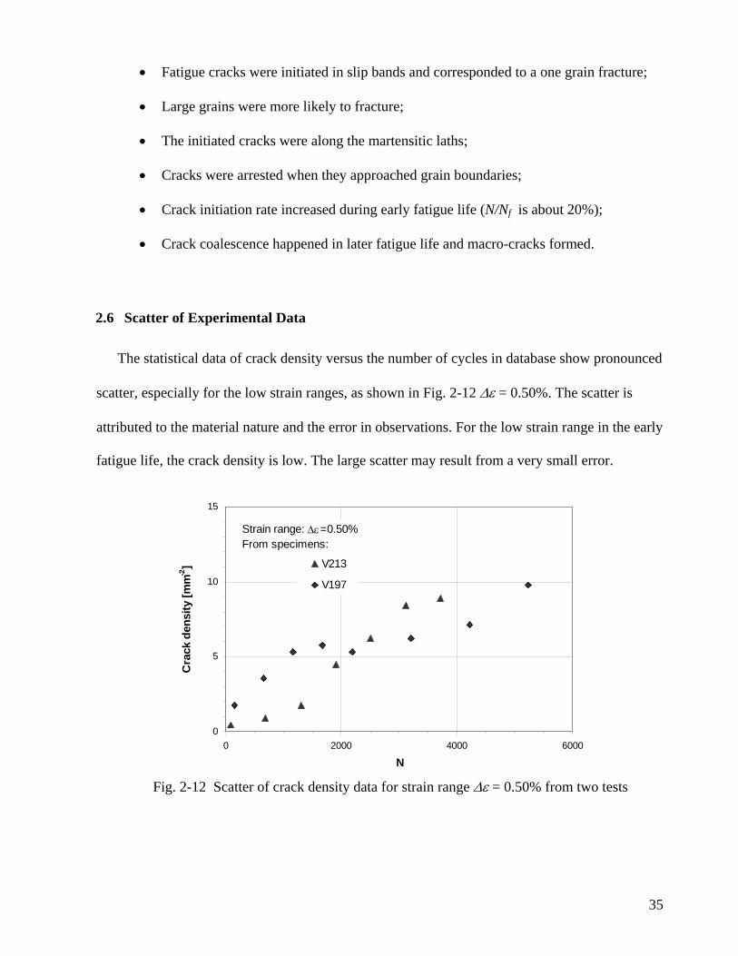
The statistical data of crack density versus the number of cycles in database show pronounced
scatter, especially for the low strain ranges, as shown in Fig. 2-12 ∆ε = 0.50%. The scatter is
attributed to the material nature and the error in observations. For the low strain range in the early
fatigue life, the crack density is low. The large scatter may result from a very small error.
Strain range: ∆ε=0.50%From specimens:
0
5
10
15
0 2000 4000 6000
N
Cra
ck d
ensi
ty [m
m-2
] V213
V197
Fig. 2-12 Scatter of crack density data for strain range ∆ε = 0.50% from two tests
35
For high strain ranges, such as ∆ε = 0.80% and 0.90%, extensive plastic deformation is
visible on the specimen surface, as can be found in Fig. 2-8 (c). The pictures taken under
microscope show an abundance of crack-like patterns. But there is no unambiguous procedure to
distinguish an extrusion from a crack at the given degree of resolution. The massive surface
roughness might lead to the unreliable statistical data of crack initiation which are the basis of
simulation. Therefore the simulation will mainly aim at the crack initiation process at the low and
intermediate strain ranges.
36
CHAPTER 3 IDEAS AND HYPOTHESES OF MODELING
As explained in the preceding chapter, the studied material, F82H, shows multiple crack
initiation. The underlying microstructure is critical to the crack initiation behavior. Hence,
simulation models are developed which can take the influences of microstructure factors and
microscopic material properties into account. In the present research, the term crack initiation
means that a single one-segment crack appears in a grain. The crack initiation process means the
fatigue stage in which the microcracks initiate continuously with fatigue cycles.
3.1 Material Model
The present study will focus on the effects of microstructural factors, such as slip systems,
grain sizes and grain orientations, on the fatigue crack initiation. A stochastic model with
irregular shaped mosaic seems a suitable one. Among the available models, the Voronoi
tessellation can represent microstructure in a more general sense. Therefore the stochastic grain
aggregates of representative volume element (RVE) are generated by Voronoi process to
represent the microstructures of the studied material.
In the Voronoi model, the material is assumed to be elastic with anisotropic stress-strain
relation using single crystal material parameters. The stress distribution will be analyzed by a
general-purpose finite element code ABAQUS. In this way the grain misorientation effect, i.e.
the inhomogeneous local stress distribution induced by deformation incompatibility and its
influence on the crack initiation, can be investigated. After a crack is initiated the stress
concentration near crack tips and stress relief along crack surfaces will disturb the original stress
37
field of the uncracked RVE. In the present study, the local stress redistribution after each initiated
crack will be taken into account. The same procedures are applied to the models with elasto-
plastic material properties.
The simulations are composed of two-dimensional and three-dimensional models. In the two-
dimensional models both plane-stress and plane-strain conditions will be applied. In order to
study the effects of the three-dimensional slip systems and the three-dimensional stress state, a
three-dimensional FE analysis is carried out.
3.2 Fatigue Model
As reviewed in Chapter 1, there are only a few microstructure-based models available in
literature. According to the characteristics of the initiation of microcracks observed on the
specimen surfaces, a large amount of PSBs was found and the micro-cracks were considered to
initiate in these PSBs. Moreover the initiated cracks were mostly oriented in ±45° to the loading
axis. This indicates that the mechanism of crack initiation is a shear-controlled slip-band mode,
which is in agreement with the Tanaka-Mura model and its extended version, the Chan model.
One advantage of the two models is that the main influencing factors such as microstructure
parameters, loading conditions and material properties can be taken into account. Since the PSB
appears mainly on slip planes oriented for single slip, the assumption that a crack initiates along
the primary slip system is reasonable. As pointed out in [21], however, the dislocation movement
is assumed to be fully irreversible but it is not the case in the real material.
In the present study, the damage accumulation in early fatigue life of F82H is assumed to be a
one by one crack initiation process. The Tanaka-Mura model and the Chan model will be used to
determine the crack initiation life ∆Ni of the potential cracks. Among all the potential cracks, the
one with the minimum number of cycles to crack initiation, ∆Nmin, will be the first initiated crack,
∆Nmin=Minimum(∆N1, ∆N2, … ∆Nm) (3-1)
38
where ∆N1, ∆N2, … ∆Nm are the numbers of cycles of potential cracks and m is the number of
potential cracks in a model. This simulation method is considered to be very similar to the natural
process of crack initiation in the material.
3.3 Parameter Studies
3.3.1 Critical Shear Stress Study
Although numerous experimental data can be found in the database or in literature, some
parameters, which are not common, are usually not available. In the present study one parameter
is the critical shear stress τc, which is an influencing parameter in the Tanaka-Mura and the Chan
predictions. In this case, an estimation method from experimental data was developed. In the
work of Hoshide [4], the critical shear stress τc was estimated from the experimental data of pure
torsion fatigue. The shear stress ∆τ and the number of cycles Nc in Eq. (1-4) were replaced by the
endurance limit of torsion fatigue τe and the corresponding cycles Ne (Ne = 106). When other
material parameters were determined, then τc could be calculated by Eq. (3-2), leading to a value
of 108 MPa for a carbon steel with 0.37wt%C [41] and a value of 146 MPa for a SAE 1045
normalized steel [4].
e
sec Nd
GW⋅⋅−
−=)1(
821
νπττ (3-2)
As no torsion data were available, the critical shear stress τc in the present work is estimated
as follows: First, the fatigue limit σ-1 is determined by extrapolating the stress amplitude (in
Table 2-4) to fatigue life of N = 106; then the corresponding τ-1 is assumed to be half of the
magnitude of σ-1. By substituting τ-1 for τe, N for Ne and other material constants for the
parameters in Eq. (3-2), τc is determined. The obtained τc for the studied material F82H is 103
MPa when the data in the database are used. With the same procedures as above, the estimated τc
39
from the fatigue data at room temperature [66] (the same material) is 147 MPa. These results
suggest that the τc determined in Eq. (3-2) is very sensitive to the database and its inherent
scatter. Failure criterion of fatigue gives very little difference in Nf, therefore again the τc
estimated by this method is not valid. In order to find the most reasonable value of τc, a
parameter study is carried out and the variation of crack initiation life with τc is investigated. The
method and results are presented in Chapter 5.
3.3.2 Microstructure Parameter Study
As it is well known, the scatter of fatigue life can be rather large. The statistical data in the
database also show a large scatter. The reasons are attributed to the inhomogeneity of material,
the experimental conditions and errors in measurement or observation. Since crack initiation is
related to the characteristics of microstructure, such as grain sizes and orientations, the scatter of
crack initiation life may result from the difference of the microstructure details. For example, the
crack initiation in a large grain with slip plane oriented at 45° is very likely. If the significant
scatter occurs to the simulation model, it may influence simulation results. Therefore, a few
models with different grain structures and orientations are created and the same simulation
procedure is applied repeatedly.
40
CHAPTER 4 CONSTRUCTION OF SIMULATION MODELS
All aspects associated with the construction of the simulation models in the study are
presented in this chapter. The ideas how to generate simulation models are introduced in Section
4.1. In Section 4.2 the details about microstructure modeling are described. Section 4.3 introduces
the strategies of Finite Element (FE) analyses, which were performed by a general-purpose FE
code, ABAQUS/Standard. The description of the material properties of models can be found in
Section 4.4. The procedure to simulate fatigue crack initiation process, based on the dislocation
pile-up mechanism, is described in Section 4.5. Before the simulation is applied, the validity of the
two-dimensional and three-dimensional representative volume element models (2D-RVE and 3D-
RVE) generated by Voronoi processes is checked. The ideas and results are described in Section
4.6.
4.1 Model Outline
The model used in the present study is a kind of mesoscopic one based on the representative
volume element (RVE), which represents a grain aggregate and allows microstructural parameters
to be introduced. The RVE represents a material point and its neighborhood in the middle of a
specimen and on the top surface. The simulation is started from a two-dimensional model with
orthotropic elastic material properties.
41
The grain structure is generated by a specially designed two-dimensional Voronoi process. The
generated Voronoi tessellation is a subset in which all angles within polygons exceed 30º and the
maximum aspect ratio of the longest to the shortest line within a single polygon is lower than a
critical value [60]. These features make the geometrical configuration of Voronoi cells suitable for
FE meshing and more similar to the real prior austenite grains in F82H steel.
In the two-dimensional RVE model (2D-RVE) a random number representing an angle is
attributed to each Voronoi cell and the angle defines the orientation of the crystal lattice on the
plane, whereas in the three-dimensional RVE (3D-RVE) the orientation for each grain is
determined by the three Eulerian rotation angles obtained from a random number generator. Elastic
orthotropic property of single crystal is assumed. Based on the created model, the inhomogeneous
stress distribution induced by grain misorientation will be simulated by finite element analyses.
Potential crack paths (PCP) have to be defined in the random grain structure in order to
simulate the crack initiation process. A PCP of each grain is the trace of one of its slip planes,
which coincide with martensitic laths. In the present simulation it is assumed that one prior
austenite grain consists of only one packet of parallel martensitic laths. A PCP represents a will-be
crack and only the PCP can become a ‘real’ crack, when the crack initiation criterion is satisfied. It
is assumed that the number of load cycles needed to grow a crack to the first barrier is small
compared to the number of load cycles to crack initiation. Therefore, once a crack is initiated, it
will immediately grow to the grain boundary. Stable crack growth within one grain is not modeled.
A three-dimensional model with random grain structure is quite a complex problem to solve. If
cracks are introduced the model complexity increases considerably. One has to take into account
the extension of the grains in depth and their three-dimensional orientations. These requirements
lead, consequently, to a dramatic increase in computational costs. There are two possible
simplifications of the fully-fledged three-dimensional random grain structure. One of the obvious
42
choices is to restrict the simulation to a few cells which may contain one or two cracks but this
does not allow the modeling of the continuous damage accumulation process, which can be
compared to experimental data. Another possibility is to take a thin layer of elements on the
surface which are connected to the bulk material. This model does not take into account the grain
configuration varying in depth direction which, in turn, will influence the damage accumulation
process on the surface. However, it does allow a study of the effect of the spatial grain orientation
and the effect of the three-dimensional stress state in addition to the damage accumulation by
continuous crack initiation. The latter approach is used in this study.
The material law for the FE simulation, either completely orthotropic elastic or orthotropic
elastic-isotropic plastic, is used for both the 2D-RVE and 3D-RVE models. The Tanaka-Mura
equation and the Chan equation are chosen as the fatigue prediction models.
4.2 Representative Volume Element Model
4.2.1 Determination of Slip System
The crystal lattice of martensite is formed by transforming an original face centred cubic (fcc)
lattice of austenite to a body centred tetragonal (bct) with a rapid cooling rate [67] during the heat-
treatment. The cooling rate is so high that the interstitial carbon atoms have no time to escape from
the lattice and remain in the common octahedral sites of bcc and fcc, as shown in Fig. 4- 1.
The tetragonality of martensite of plain carbon steels, however, is the function of the carbon
content. The lattice constants a and c vary with carbon content. The numerical relation is shown in
Eq. (4-1):
)(045.0005.1/ Cwac += (4-1)
43
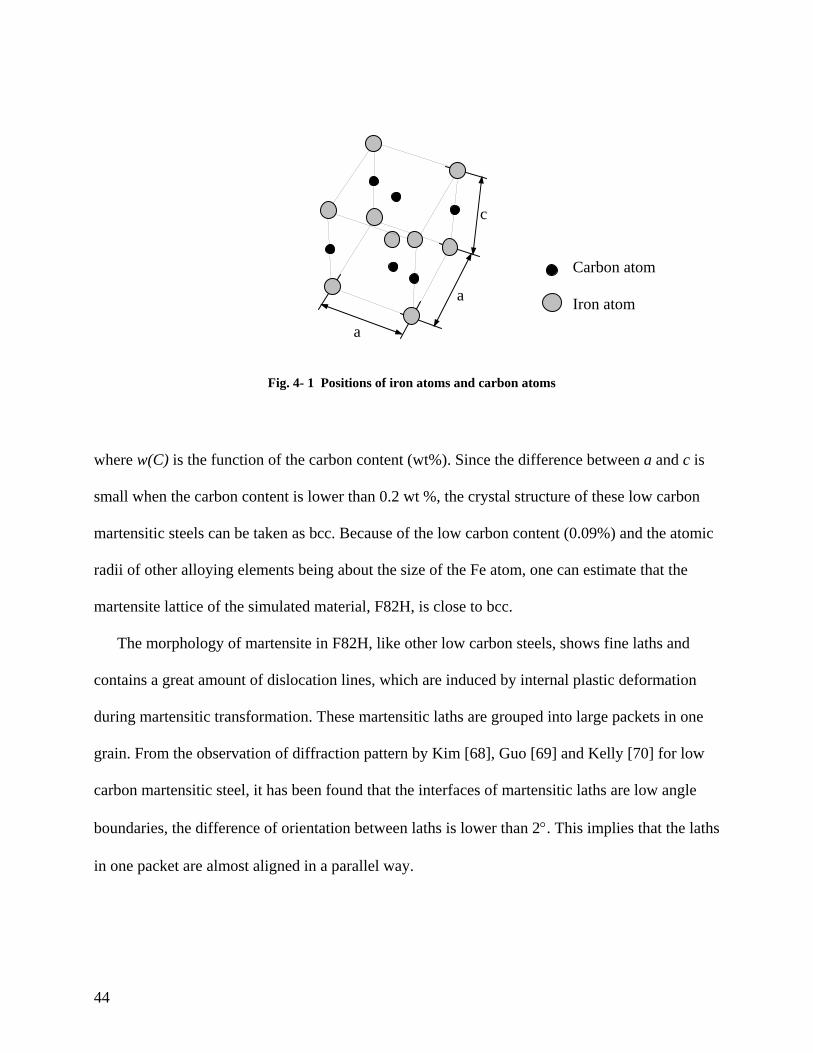
Fig. 4- 1 Positions of iron atoms and carbon atoms
where w(C) is the function of the carbon content (wt%). Since the difference between a and c is
small when the carbon content is lower than 0.2 wt %, the crystal structure of these low carbon
martensitic steels can be taken as bcc. Because of the low carbon content (0.09%) and the atomic
radii of other alloying elements being about the size of the Fe atom, one can estimate that the
martensite lattice of the simulated material, F82H, is close to bcc.
The morphology of martensite in F82H, like other low carbon steels, shows fine laths and
contains a great amount of dislocation lines, which are induced by internal plastic deformation
during martensitic transformation. These martensitic laths are grouped into large packets in one
grain. From the observation of diffraction pattern by Kim [68], Guo [69] and Kelly [70] for low
carbon martensitic steel, it has been found that the interfaces of martensitic laths are low angle
boundaries, the difference of orientation between laths is lower than 2°. This implies that the laths
in one packet are almost aligned in a parallel way.
c
a
a
Carbon atom Iron atom
44
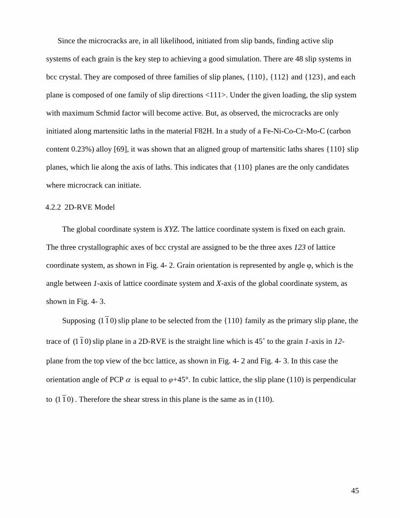
Since the microcracks are, in all likelihood, initiated from slip bands, finding active slip
systems of each grain is the key step to achieving a good simulation. There are 48 slip systems in
bcc crystal. They are composed of three families of slip planes, {110}, {112} and {123}, and each
plane is composed of one family of slip directions <111>. Under the given loading, the slip system
with maximum Schmid factor will become active. But, as observed, the microcracks are only
initiated along martensitic laths in the material F82H. In a study of a Fe-Ni-Co-Cr-Mo-C (carbon
content 0.23%) alloy [69], it was shown that an aligned group of martensitic laths shares {110} slip
planes, which lie along the axis of laths. This indicates that {110} planes are the only candidates
where microcrack can initiate.
4.2.2 2D-RVE Model
The global coordinate system is XYZ. The lattice coordinate system is fixed on each grain.
The three crystallographic axes of bcc crystal are assigned to be the three axes 123 of lattice
coordinate system, as shown in Fig. 4- 2. Grain orientation is represented by angle φ, which is the
angle between 1-axis of lattice coordinate system and X-axis of the global coordinate system, as
shown in Fig. 4- 3.
Supposing )011( slip plane to be selected from the {110} family as the primary slip plane, the
trace of )011( slip plane in a 2D-RVE is the straight line which is 45˚ to the grain 1-axis in 12-
plane from the top view of the bcc lattice, as shown in Fig. 4- 2 and Fig. 4- 3. In this case the
orientation angle of PCP α is equal to φ+45°. In cubic lattice, the slip plane (110) is perpendicular
to )011( . Therefore the shear stress in this plane is the same as in (110).
45
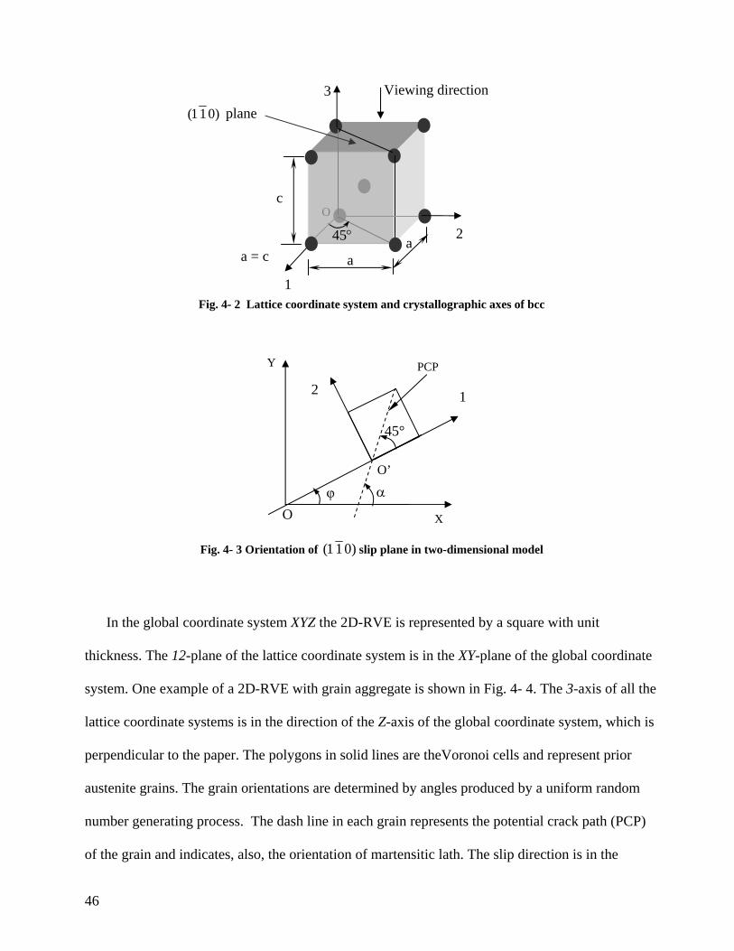
Fig. 4- 2 Lattice coordinate system and crystallographic axes of bcc
Fig. 4- 3 Orientation of )011( slip plane in two-dimensional model
In the global coordinate system XYZ the 2D-RVE is represented by a square with unit
thickness. The 12-plane of the lattice coordinate system is in the XY-plane of the global coordinate
system. One example of a 2D-RVE with grain aggregate is shown in Fig. 4- 4. The 3-axis of all the
lattice coordinate systems is in the direction of the Z-axis of the global coordinate system, which is
perpendicular to the paper. The polygons in solid lines are theVoronoi cells and represent prior
austenite grains. The grain orientations are determined by angles produced by a uniform random
number generating process. The dash line in each grain represents the potential crack path (PCP)
of the grain and indicates, also, the orientation of martensitic lath. The slip direction is in the
a = c
c
aa
3
245°
Viewing direction
O
1
)011( plane
X
Y
1 2
O
PCP
O’
α
45°
φ
46
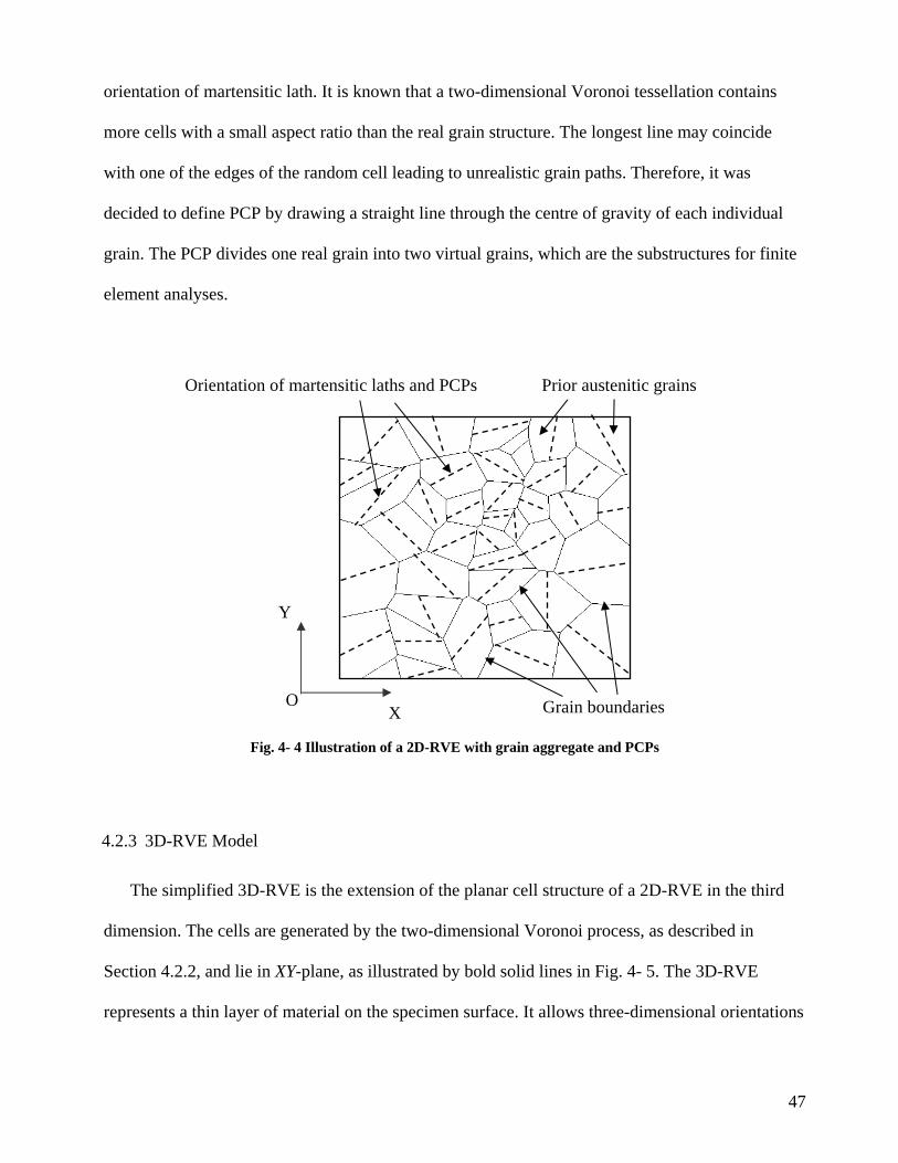
Orientation of martensitic laths and PCPs Prior austenitic grains
Grain boundaries O
orientation of martensitic lath. It is known that a two-dimensional Voronoi tessellation contains
more cells with a small aspect ratio than the real grain structure. The longest line may coincide
with one of the edges of the random cell leading to unrealistic grain paths. Therefore, it was
decided to define PCP by drawing a straight line through the centre of gravity of each individual
grain. The PCP divides one real grain into two virtual grains, which are the substructures for finite
element analyses.
Fig. 4- 4 Illustration of a 2D-RVE with grain aggregate and PCPs
Y
X
4.2.3 3D-RVE Model
The simplified 3D-RVE is the extension of the planar cell structure of a 2D-RVE in the third
dimension. The cells are generated by the two-dimensional Voronoi process, as described in
Section 4.2.2, and lie in XY-plane, as illustrated by bold solid lines in Fig. 4- 5. The 3D-RVE
represents a thin layer of material on the specimen surface. It allows three-dimensional orientations
47
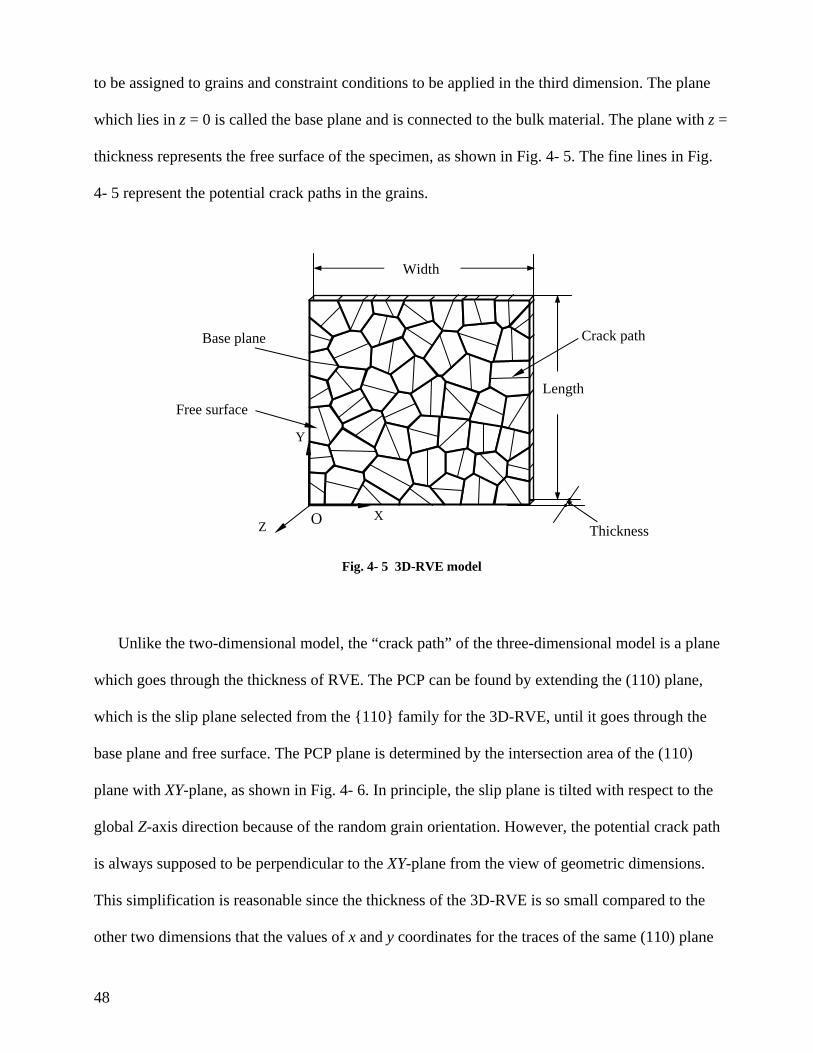
to be assigned to grains and constraint conditions to be applied in the third dimension. The plane
which lies in z = 0 is called the base plane and is connected to the bulk material. The plane with z =
thickness represents the free surface of the specimen, as shown in Fig. 4- 5. The fine lines in Fig.
4- 5 represent the potential crack paths in the grains.
Fig. 4- 5 3D-RVE model
Unlike the two-dimensional model, the “crack path” of the three-dimensional model is a plane
which goes through the thickness of RVE. The PCP can be found by extending the (110) plane,
which is the slip plane selected from the {110} family for the 3D-RVE, until it goes through the
base plane and free surface. The PCP plane is determined by the intersection area of the (110)
plane with XY-plane, as shown in Fig. 4- 6. In principle, the slip plane is tilted with respect to the
global Z-axis direction because of the random grain orientation. However, the potential crack path
is always supposed to be perpendicular to the XY-plane from the view of geometric dimensions.
This simplification is reasonable since the thickness of the 3D-RVE is so small compared to the
other two dimensions that the values of x and y coordinates for the traces of the same (110) plane
Width
Length
Thickness
Free surface
O
Y
X
Crack path Base plane
Z
48

on the base plane and on free surface are almost the same. The approximation simplifies the model
creation and the finite element analyses. This simplification, however, is not applied to the stress
analyses on the plane of crack path. In other words, the stress components on PCP planes are
presented in three-dimensional space and are associated with the grain orientations.
Fig. 4- 6 Scheme of the potential crack paths of 3D-RVE
1
3
2
X
Z
Yoo
PCP plane
(110) plane
4.2.4 RVE Size and Voronoi Boundary Effects
Generally speaking, the number of grains in an RVE is not limited. The minimum number of
grains required in a model depends on the following conditions.
(i) The effective number of grains Ne in a Voronoi model is smaller than the given number
of grains N. The phrase of ‘effective number’ means the number of grains which are not
on model boundaries and ‘given number’ means the total number of grains in a model.
The shapes of the grains on model boundaries are different from the grains inside the
models. From the statistics of the numbers of Ne and N, it is found that the fraction of
Ne /N decreases with N increasing, as shown in Fig. 4- 7. Because the area of grains on
49
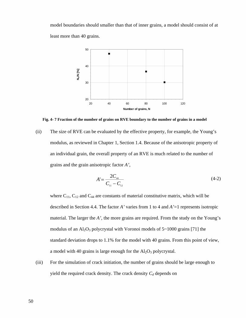
model boundaries should smaller than that of inner grains, a model should consist of at
least more than 40 grains.
20
30
40
50
20 40 60 80 100 120
Number of grains, N
Ne/N
[%]
Fig. 4- 7 Fraction of the number of grains on RVE boundary to the number of grains in a model
(ii) The size of RVE can be evaluated by the effective property, for example, the Young’s
modulus, as reviewed in Chapter 1, Section 1.4. Because of the anisotropic property of
an individual grain, the overall property of an RVE is much related to the number of
grains and the grain anisotropic factor A’,
1211
442'CC
CA−
= (4-2)
where C11, C12 and C44 are constants of material constitutive matrix, which will be
described in Section 4.4. The factor A’ varies from 1 to 4 and A’=1 represents isotropic
material. The larger the A’, the more grains are required. From the study on the Young’s
modulus of an Al2O3 polycrystal with Voronoi models of 5~1000 grains [71] the
standard deviation drops to 1.1% for the model with 40 grains. From this point of view,
a model with 40 grains is large enough for the Al2O3 polycrystal.
(iii) For the simulation of crack initiation, the number of grains should be large enough to
yield the required crack density. The crack density Cd depends on
50
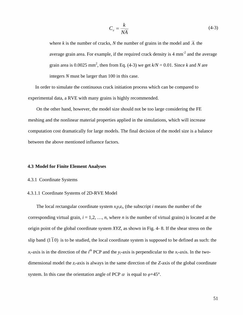
ANkCd = (4-3)
where k is the number of cracks, N the number of grains in the model and A the
average grain area. For example, if the required crack density is 4 mm-2 and the average
grain area is 0.0025 mm2, then from Eq. (4-3) we get k/N = 0.01. Since k and N are
integers N must be larger than 100 in this case.
In order to simulate the continuous crack initiation process which can be compared to
experimental data, a RVE with many grains is highly recommended.
On the other hand, however, the model size should not be too large considering the FE
meshing and the nonlinear material properties applied in the simulations, which will increase
computation cost dramatically for large models. The final decision of the model size is a balance
between the above mentioned influence factors.
4.3 Model for Finite Element Analyses
4.3.1 Coordinate Systems
4.3.1.1 Coordinate Systems of 2D-RVE Model
The local rectangular coordinate system xiyizi, (the subscript i means the number of the
corresponding virtual grain, i = 1,2, …, n, where n is the number of virtual grains) is located at the
origin point of the global coordinate system XYZ, as shown in Fig. 4- 8. If the shear stress on the
slip band )011( is to be studied, the local coordinate system is supposed to be defined as such: the
xi-axis is in the direction of the ith PCP and the yi-axis is perpendicular to the xi-axis. In the two-
dimensional model the zi-axis is always in the same direction of the Z-axis of the global coordinate
system. In this case the orientation angle of PCP α is equal to φ+45°.
51
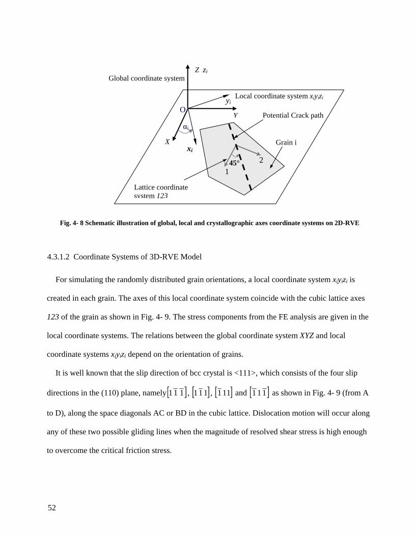
Fig. 4- 8 Schematic illustration of global, local and crystallographic axes coordinate systems on 2D-RVE
X
Global coordinate system
Grain i
Lattice coordinate system 123
Y
Z zi
xi
yi
45° 1
2
Local coordinate system xiyizi
Potential Crack path O
αi
4.3.1.2 Coordinate Systems of 3D-RVE Model
For simulating the randomly distributed grain orientations, a local coordinate system xiyizi is
created in each grain. The axes of this local coordinate system coincide with the cubic lattice axes
123 of the grain as shown in Fig. 4- 9. The stress components from the FE analysis are given in the
local coordinate systems. The relations between the global coordinate system XYZ and local
coordinate systems xiyizi depend on the orientation of grains.
It is well known that the slip direction of bcc crystal is <111>, which consists of the four slip
directions in the (110) plane, namely [ ]111 , [ ]111 , [ ]111 and [ ]111 as shown in Fig. 4- 9 (from A
to D), along the space diagonals AC or BD in the cubic lattice. Dislocation motion will occur along
any of these two possible gliding lines when the magnitude of resolved shear stress is high enough
to overcome the critical friction stress.
52
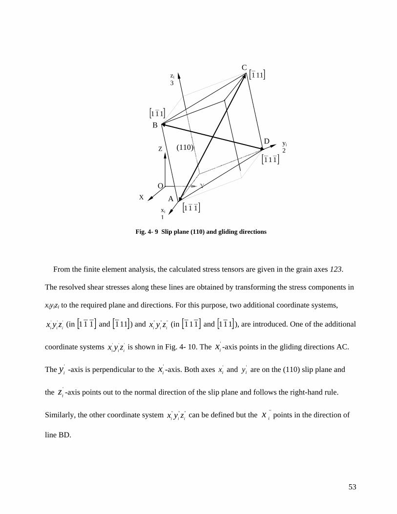
Fig. 4- 9 Slip plane (110) and gliding directions
From the finite element analysis, the calculated stress tensors are given in the grain axes 123.
The resolved shear stresses along these lines are obtained by transforming the stress components in
xiyizi to the required plane and directions. For this purpose, two additional coordinate systems,
(in '''iii zyx [ ]111 and [ ]111 ) and (in ''''''
iii zyx [ ]111 and [ ]111 ), are introduced. One of the a
coordinate systems '''iii zyx is shown in Fig. 4- 10. The '
ix -axis poi s in the gliding directions A
The 'iy -axis is perpendicular to the '
ix -axis. Both axes 'ix and '
iy are on the (110) slip plane and
the 'iz -axis points out to the normal direction of the slip plane and follows the right-hand rule.
Similarly, the other coordinate system ''''''iii zyx can be defined but the ''
ix points e direction of
line BD.
dditional
nt C.
in th
Y
Z
xi 1
zi 3
[ ]111
[ ]111
[ ]111
D
A
C
B
O
[ ]111
(110) yi 2
X
53
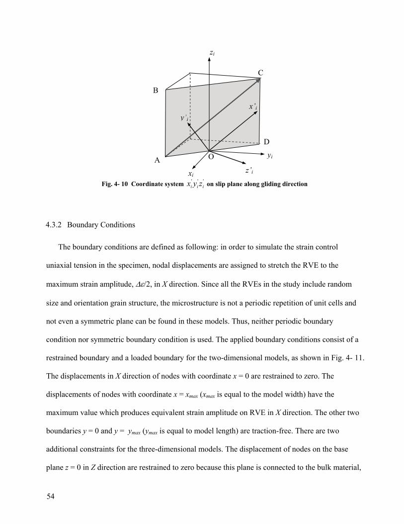
Fig. 4- 10 Coordinate system on slip plane along gliding direction'''iii zyx
D
C
O
z’i
y’ix’i
zi
xi
B
yiA
4.3.2 Boundary Conditions
The boundary conditions are defined as following: in order to simulate the strain control
uniaxial tension in the specimen, nodal displacements are assigned to stretch the RVE to the
maximum strain amplitude, /2, in X direction. Since all the RVEs in the study include random
size and orientation grain structure, the microstructure is not a periodic repetition of unit cells and
not even a symmetric plane can be found in these models. Thus, neither periodic boundary
condition nor symmetric boundary condition is used. The applied boundary conditions consist of a
restrained boundary and a loaded boundary for the two-dimensional models, as shown in Fig. 4- 11.
The displacements in X direction of nodes with coordinate x = 0 are restrained to zero. The
displacements of nodes with coordinate x = xmax (xmax is equal to the model width) have the
maximum value which produces equivalent strain amplitude on RVE in X direction. The other two
boundaries y = 0 and y = ymax (ymax is equal to model length) are traction-free. There are two
additional constraints for the three-dimensional models. The displacement of nodes on the base
plane z = 0 in Z direction are restrained to zero because this plane is connected to the bulk material,
54
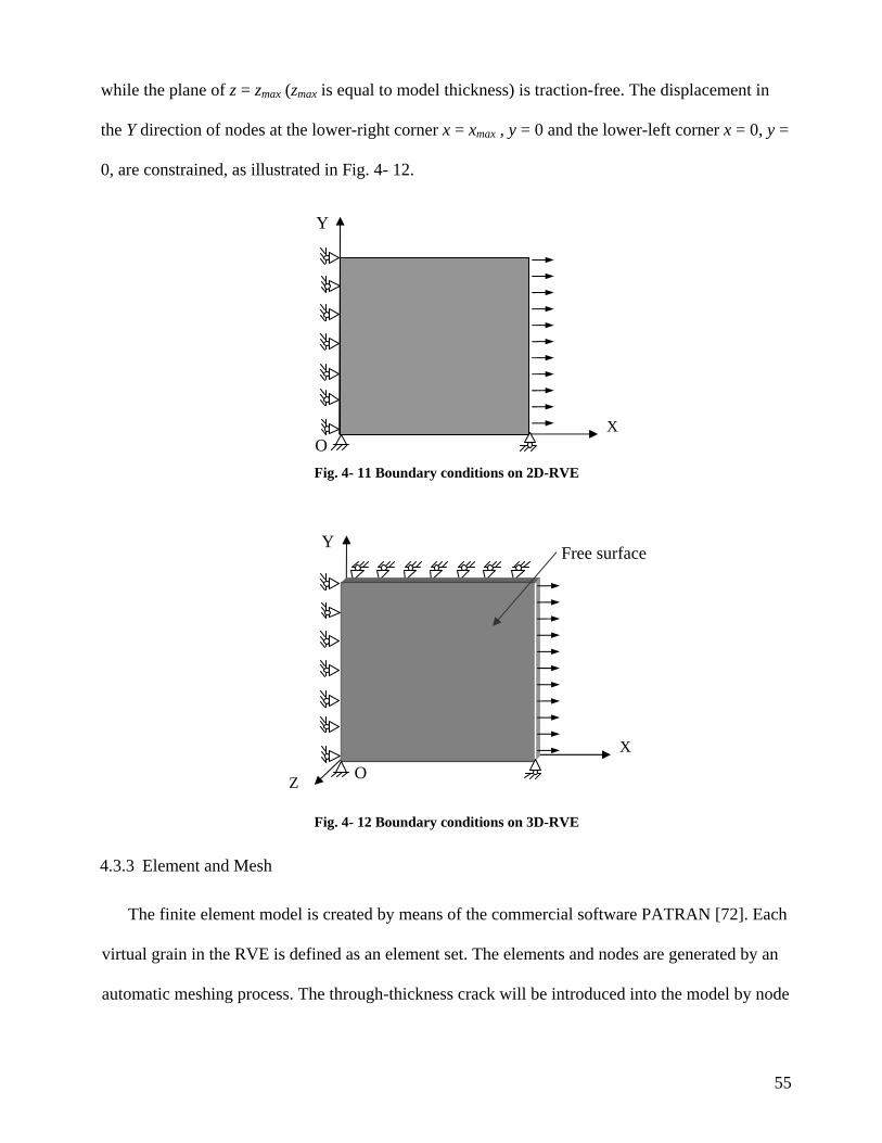
while the plane of z = zmax (zmax is equal to model thickness) is traction-free. The displacement in
the Y direction of nodes at the lower-right corner x = xmax , y = 0 and the lower-left corner x = 0, y =
0, are constrained, as illustrated in Fig. 4- 12.
Fig. 4- 11 Boundary conditions on 2D-RVE
Fig. 4- 12 Boundary conditions on 3D-RVE
Y
O X
X
Y
O
Free surface
Z
4.3.3 Element and Mesh
The finite element model is created by means of the commercial software PATRAN [72]. Each
virtual grain in the RVE is defined as an element set. The elements and nodes are generated by an
automatic meshing process. The through-thickness crack will be introduced into the model by node
55
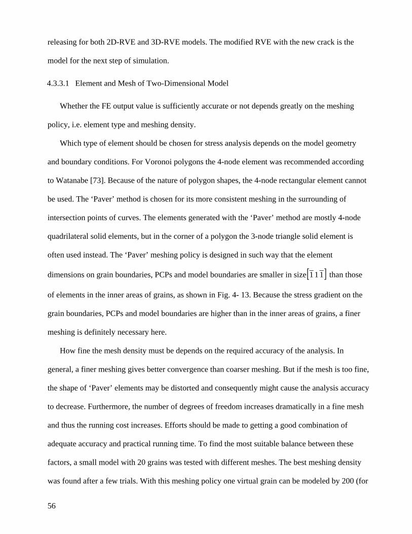
releasing for both 2D-RVE and 3D-RVE models. The modified RVE with the new crack is the
model for the next step of simulation.
4.3.3.1 Element and Mesh of Two-Dimensional Model
Whether the FE output value is sufficiently accurate or not depends greatly on the meshing
policy, i.e. element type and meshing density.
Which type of element should be chosen for stress analysis depends on the model geometry
and boundary conditions. For Voronoi polygons the 4-node element was recommended according
to Watanabe [73]. Because of the nature of polygon shapes, the 4-node rectangular element cannot
be used. The ‘Paver’ method is chosen for its more consistent meshing in the surrounding of
intersection points of curves. The elements generated with the ‘Paver’ method are mostly 4-node
quadrilateral solid elements, but in the corner of a polygon the 3-node triangle solid element is
often used instead. The ‘Paver’ meshing policy is designed in such way that the element
dimensions on grain boundaries, PCPs and model boundaries are smaller in size [ ]111 than those
of elements in the inner areas of grains, as shown in Fig. 4- 13. Because the stress gradient on the
grain boundaries, PCPs and model boundaries are higher than in the inner areas of grains, a finer
meshing is definitely necessary here.
How fine the mesh density must be depends on the required accuracy of the analysis. In
general, a finer meshing gives better convergence than coarser meshing. But if the mesh is too fine,
the shape of ‘Paver’ elements may be distorted and consequently might cause the analysis accuracy
to decrease. Furthermore, the number of degrees of freedom increases dramatically in a fine mesh
and thus the running cost increases. Efforts should be made to getting a good combination of
adequate accuracy and practical running time. To find the most suitable balance between these
factors, a small model with 20 grains was tested with different meshes. The best meshing density
was found after a few trials. With this meshing policy one virtual grain can be modeled by 200 (for
56
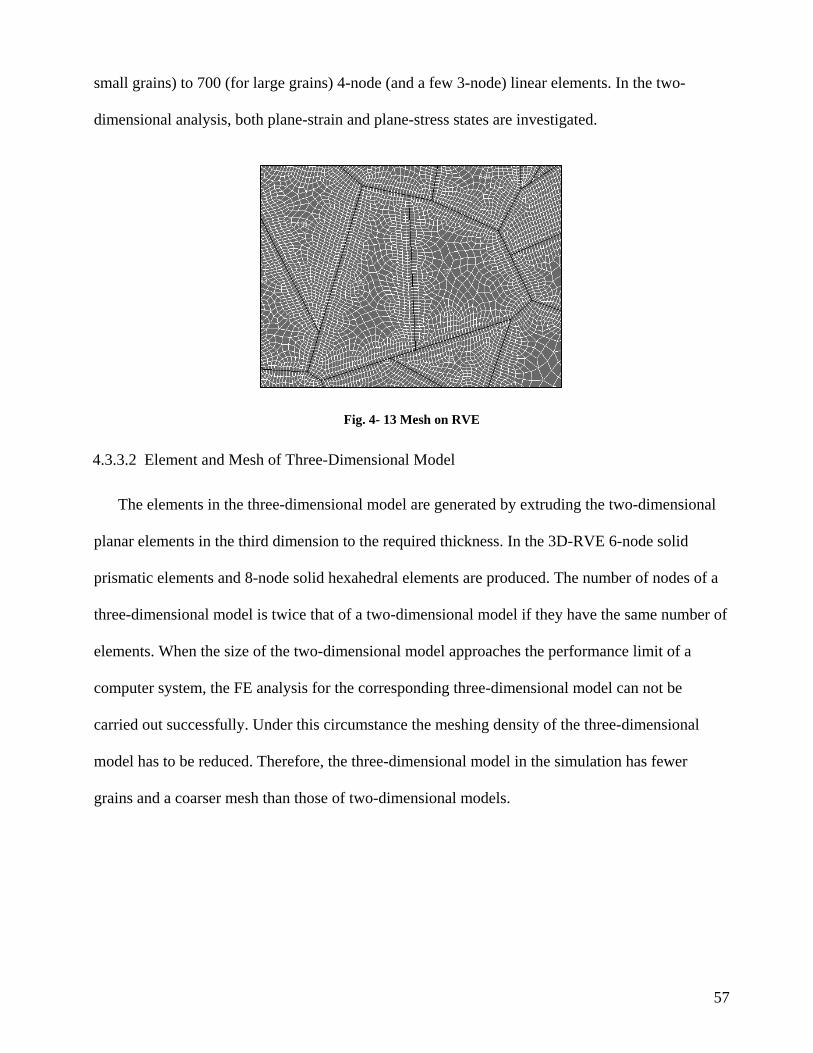
small grains) to 700 (for large grains) 4-node (and a few 3-node) linear elements. In the two-
dimensional analysis, both plane-strain and plane-stress states are investigated.
Fig. 4- 13 Mesh on RVE
4.3.3.2 Element and Mesh of Three-Dimensional Model
The elements in the three-dimensional model are generated by extruding the two-dimensional
planar elements in the third dimension to the required thickness. In the 3D-RVE 6-node solid
prismatic elements and 8-node solid hexahedral elements are produced. The number of nodes of a
three-dimensional model is twice that of a two-dimensional model if they have the same number of
elements. When the size of the two-dimensional model approaches the performance limit of a
computer system, the FE analysis for the corresponding three-dimensional model can not be
carried out successfully. Under this circumstance the meshing density of the three-dimensional
model has to be reduced. Therefore, the three-dimensional model in the simulation has fewer
grains and a coarser mesh than those of two-dimensional models.
57
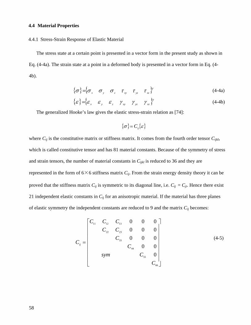
4.4 Material Properties
4.4.1 Stress-Strain Response of Elastic Material
The stress state at a certain point is presented in a vector form in the present study as shown in
Eq. (4-4a). The strain state at a point in a deformed body is presented in a vector form in Eq. (4-
4b).
{ } { }Txzyzxyzyx τττσσσσ = (4-4a)
{ } { }Txzyzxyzyx γγγεεεε = (4-4b)
The generalized Hooke’s law gives the elastic stress-strain relation as [74]:
{ } { }εσ ijC=
where Cij is the constitutive matrix or stiffness matrix. It comes from the fourth order tensor Cijkl,
which is called constitutive tensor and has 81 material constants. Because of the symmetry of stress
and strain tensors, the number of material constants in Cijkl is reduced to 36 and they are
represented in the form of 6×6 stiffness matrix Cij. From the strain energy density theory it can be
proved that the stiffness matrix Cij is symmetric to its diagonal line, i.e. Cij = Cji. Hence there exist
21 independent elastic constants in Cij for an anisotropic material. If the material has three planes
of elastic symmetry the independent constants are reduced to 9 and the matrix Cij becomes:
(4-5) ⎥⎢ 000C
⎥⎥⎥⎥
⎥⎥
⎦
⎤
⎢⎢⎢⎢
⎢⎢
⎣
⎡
=
66
55
44
33
2322
131211
000
000000
CCsym
C
CCCCC
Cij
58
The material with three symmetric planes is called orthotropic material, which displays different
values of stiffness in mutually perpendicular directions. If the crystal has more symmetric planes,
there are fewer constants in matrix Cij. There are three independent constants in a cubic crystal.
In this study the linear elastic stress-strain response of individual grains of the investigated
material is assumed to be orthotropic. The components of Eq. (4-5) are chosen from the material
stiffness matrix of a single crystal pure iron [75]: C11 = C22 = C33 = 233 GPa, C12 = C13 = C23 =
135 GPa, C44 = C55 = C66 = 118 GPa.
In the FE analysis code ABAQUS, the local coordinate systems are designed to define the
material orientation and the output stress (strain) components. When the local coordinate system is
defined at the slip direction (i.e. not at the lattice coordinate system), for example, a transformation
of the stiffness matrix is imposed. The transformation matrix between two coordinate systems is
described in Appendix A1.
4.4.2 Stress-Strain Response of Elasto-Plastic Material
Experiments showed non-linear stress-strain curves with pronounced plastic deformation for
most strain ranges for F82H steel. Therefore, a purely elastic simulation does not seem to be
appropriate. An elasto-plastic response is selected for the present simulations. In order to
distinguish between the contributions of elastic and plastic deformation, the elasto-plastic material
behaviour is approximately described by a piecewise linear stress-strain curve.
In many cases, the elasto-plastic response of ductile metals can be simplified into three parts,
one elastic part, one hardening plasticity part and a perfect plasticity part. One typical example is
shown schematically in Fig. 4-14. The bold solid line represents the stress-strain curve of a
material obtained from a tension test. E is the Young’s modulus, E’ is the tangential modulus of the
linear hardening plasticity, σy0 is the stress where plastic deformation appears and σu is the stress
where perfect plasticity starts.
59
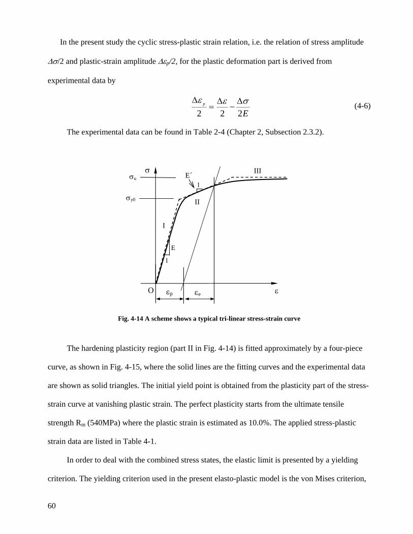
In the present study the cyclic stress-plastic strain relation, i.e. the relation of stress amplitude
∆σ/2 and plastic-strain amplitude ∆εp/2, for the plastic deformation part is derived from
experimental data by
Ep
222σεε ∆
−∆
=∆
(4-6)
The experimental data can be found in Table 2-4 (Chapter 2, Subsection 2.3.2).
Fig. 4-14 A scheme shows a typical tri-linear stress-strain curve
The hardening plasticity region (part II in Fig. 4-14) is fitted approximately by a four-piece
curve, as shown in Fig. 4-15, where the solid lines are the fitting curves and the experimental data
are shown as solid triangles. The initial yield point is obtained from the plasticity part of the stress-
strain curve at vanishing plastic strain. The perfect plasticity starts from the ultimate tensile
strength Rm (540MPa) where the plastic strain is estimated as 10.0%. The applied stress-plastic
strain data are listed in Table 4-1.
In order to deal with the combined stress states, the elastic limit is presented by a yielding
criterion. The yielding criterion used in the present elasto-plastic model is the von Mises criterion,
1
E
E´1
I
II
III
ε
σ
εeO εp
σu
σy0
60
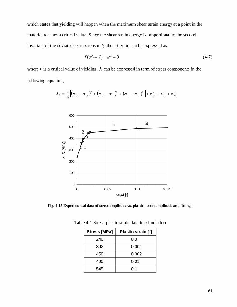
which states that yielding will happen when the maximum shear strain energy at a point in the
material reaches a critical value. Since the shear strain energy is proportional to the second
invariant of the deviatoric stress tensor J2, the criterion can be expressed as:
0)( 22 =−= κσ Jf (4-7)
whereκis a critical value of yielding. J2 can be expressed in term of stress components in the
following equation,
( ) ( ) ( )[ ] 2222222 6
1zxyzxyxzzyyxJ τττσσσσσσ +++−+−+−=
Fig. 4-15 Experimental data of stress amplitude vs. plastic-strain amplitude and fittings
Table 4-1 Stress-plastic strain data for simulation
0
100
200
300
400
500
600
0 0.005 0.01 0.015
∆εp/2 [-]
∆σ
/2 [M
Pa]
2
43
1
Stress [MPa] Plastic strain [-]
240 0.0
392 0.001
450 0.002
490 0.01
545 0.1
61
4.5 Modeling of Crack Initiation Process
4.5.1 Fatigue Model
One of the applied models in the simulation is the Tanaka-Mura equation Eq. (1-4) (see
Chapter 1 [37]). On the basis of this model, the number of cycles to crack initiation in the ith
individual grain ∆Ni can be estimated by Eq. (4-8), which is the rewritten form of Eq. (1-4).:
2)2()1(8
cresi
si
id
GWNττνπ −∆−
=∆ i = 1, 2,… n (4-8)
where, n is the number of prior austenite grains, di is the length of the ith slip band and iresτ∆ is the
resolved shear stress range on the ith slip band. The crack initiation life Nk is the sum,
∑=
∆=k
j
jik NN
1 k = 1, 2, … l (4-9)
where l is the number of simulation loops. The corresponding crack density , i.e. the number of
cracks in the unit area, is defined as,
kdC
AkC
kd = k = 1, 2, … l (4-10)
where A is the area of the model.
Similarly, the number of cycles to crack initiation can be estimated by the Chan equation
)()()2)(1(
8 2
2
2
i
i
i
i
cres
i dc
dhGN
i
⋅−∆−
=∆ττνλπ
(4-11)
where h is the width of the slip band, c is half of the length of a nucleated crack and λ is a constant
λ = 0.005. In the present study c = d/2.
4.5.2 Average Resolved Shear Stress
4.5.2.1 Transformation of Stress Tensors
62
The stress components at nodes on RVE are calculated by ABAQUS. If the local coordinate
system does not coincide with the crack path, the stress components from FE output need to
be transformed. The stress components in the two coordinate systems
iii zyx
iii zyx and can be
presented as,
'''iii zyx
{ } { }{ } { }T
xzyzxyzzyyxx
Txzyzxyzzyyxx
''''''' τττσσσσ
τττσσσσ
=
=
If the stress components in the coordinate system are known, then the stress in the
coordinate system can be calculated by a stress transformation from
iii zyx
'''iii zyx
{ } [ ]{ }σσ T=' (4-12)
where [T] is the transform matrix. More details about tensor transformation can be found in [76]
and in Appendix A2. In 2D-RVE, the shear stress xy'τ is the required component. In 3D-RVE the
stress transformation Eq. (4-12) is applied to the two slip systems and the two sets of shear stress
''' zxτ and ''' ′′′′ zxτ along the two different slip lines are computed for the subsequent analysis.
4.5.2.2 Average Resolved Shear Stress
Since the amplitude of the resolved shear stress on slip bands is inhomogeneous in the
simulation models, the average shear stress iτ on the ith PCP is taken as the resolved stress,
∫=iA
i
i
i dAzyxA
),,(1 ττ i = 1, 2, … n (4- 13)
where Ai is the area of the ith slip band and τi(x,y,z) is the shear stress distribution function on the
slip band.
63
A. Average Resolved Shear Stress of the Two-Dimensional Model
In a two-dimensional model, because of the unit thickness of the model, Eq. (4-13) becomes
∫=iL
i
i
i dLyxL
),(1 ττ (4-14)
where Li is the length of the slip band on the ith grain. The average stress iτ can be derived from a
discrete form of Eq. (4-14) as follows
∑−
=
+ ∆+
=1
1
1 )2
(1 im
jij
ijij
i
i LL
τττ
∑−
=
∆=1
1
im
jiji LL
where Li is the length of the crack path in the model, and ∆Lij the distance between two adjacent
nodes along the path on the ith PCP. The notations of τij and τij+1 represent the shear stresses at two
adjacent nodes, where j is an index and mi is the number of nodes in the ith path.
The shear stress component τij obtained from the output of FE analysis corresponds to the
applied strain amplitude in the tension part. The Tanaka-Mura equation is based on the assumption
that the compression amplitude results in the same extent of dislocation motion but in the reverse
direction. Thus the iresτ∆ in Eq. (4-8) and Eq. (4-11) refers to the whole stress range of fatigue.
Therefore, the total resolved shear stress range iresτ∆ on a PCP is equal to 2 iτ .
B. Average Resolved Shear Stress of the Three-Dimensional Model
The discrete form of Eq. (4-13) for the simplified uniform-thickness three-dimensional model
is
∑−
=∆=
1
1
1 im
jijij
i
i AA
ττ (4-15)
64
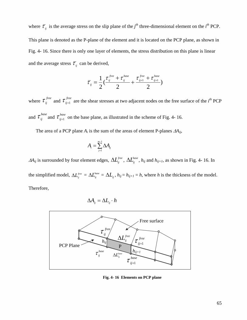
where ijτ is the average stress on the slip plane of the jth three-dimensional element on the ith PCP.
This plane is denoted as the P-plane of the element and it is located on the PCP plane, as shown in
Fig. 4- 16. Since there is only one layer of elements, the stress distribution on this plane is linear
and the average stress ijτ can be derived,
)22
(21 11
baseij
freeij
baseij
freeij
ij++ +
++
=ττττ
τ
where free
ijτ and free
ij 1+τ are the shear stresses at two adjacent nodes on the free surface of the ith P
and baseij
CP
τ and baseij 1+τ on the base plane, as illustrated in the scheme of Fig. 4- 16.
The area of a PCP plane Ai is the sum of the areas of element P-planes ∆Aij,
∑−
=
∆=1
1
m
jiji AA
∆Aij is surrounded by four element edges, freeijL∆ , base
ijL∆ , hij and hij+1, as shown in Fig. 4- 16. In
the simplified model, = = freeijL∆ base
ijL∆ ijL∆ , hij = hij+1 = h, where h is the thickness of the model.
Therefore,
hLA ijij ⋅∆=∆
Fig. 4- 16 Elements on PCP plane
Free surface
PCP Plane
freeijτ
baseij 1+τ
baseijτ
freeij 1+τ
hij+1
hij
freeijL∆
baseijL∆
P
65
It is assumed that the deformation of an element is negligible compared to the element nominal
size. Then Eq. (4-15) has the following form:
(4-16)
There are two slip directions on one PCP plane in the three-dimensional RVE. The average
shear stresses on both of the two directions are derived by Eq. (4-16). The one with the higher
value among these two average shear stresses leads to the lowest value of the number of cycles to
crack initiation and hence determines the onset of the damage accumulation process in this
particular direction.
ij
m
j
freeijijijij
⎨ ⎟⎟⎜⎜+⎟⎟= ∑freebasebase
i
i LL
i
∆⎭⎬⎫
⎩
⎧
⎠
⎞
⎝
⎛ +
⎠
⎞⎜⎜⎝
⎛ +−
=
++1
1
11
22211 ττττ
τ
4.5.3 Crack Initiation Process
The number of cycles to crack initiation ∆Ni is calculated for all potential crack paths in the
grain structure. The first micro-crack is initiated along the crack path with the shortest life, and is
introduced into the RVE model. Cracks too close to the RVE boundary have to be excluded for
stability reasons. In the next step a stress analysis is performed for the RVE with one crack.
Compared to the undamaged RVE, the average stress level drops in a displacement-controlled
situation, and the stress is redistributed in the vicinity of the cracked grain. Based on this new
stress field, the number of cycles to crack initiation is again calculated for all remaining crack
paths. As in the case of the undamaged structure, the crack path with the minimum value of the
number of cycles can be identified. Then the next crack is introduced into the RVE. The simulation
is stopped if the crack density reaches a critical value or if the FE model becomes unstable.
66
It should be noted that a crack can initiate only when the resolved shear stress range iresτ∆ is
higher than 2τc. If iresτ∆ is lower than 2τc no dislocation pile-up will occur. However the same
value of ∆Ni is obtained from Eq. (4-8) or Eq. (4-11) for negative or positive values of iresτ∆ - 2τc.
Negative values may occur if the local shear stress is low. On the other hand, if iresτ∆ is equal to 2τc
by chance, the number of cycles ∆Ni may be an infinitively large number. In order to eliminate the
possibility of incorrect results the number of cycles is set to a large value, 107, i.e. the fatigue limit,
once either of these two cases occurs.
4.5.4 Summary of Simulation Procedures and Applied Criteria
All procedures of simulation for the two- and the three-dimensional models are summarized in
the following steps:
Step 1 : Create an uncracked RVE with grain structure, PCP and material properties;
Step 2 : Create FE models with mesh and boundary conditions;
Step 3 : Run FE analysis;
Step 4 : Get output of stress components from FE data file and calculate the average shear
stress on all crack paths;
Step 5 : The number of cycles on all PCPs are calculated from Eq. (4-8) or Eq. (4-11);
Step 6 : The PCP with the minimum value of ∆Ni becomes a crack;
Step 7 : This crack is introduced into RVE and the RVE structure is modified;
Step 8 : Go to Step 3.
The above steps will be repeated until one of the following events occurs:
• The number of load cycles for the given strain amplitude reaches the preset number,
which is estimated to be more than 20% of the failure life of experimental data;
• Half of the PCPs are cracked (except the ones near to RVE edges);
67
• The number of cycles to crack initiation of all remaining PCPs are larger than 107;
• The model becomes unstable.
The next two steps deal with the data processing of simulation results:
Step 9 : The crack density versus the number of cycles is derived from Eq. (4-9) and Eq. (4-
10), respectively;
Step 10 : The stress distribution is obtained by using the PATRAN post-process from the
output file of the finite element program.
4.6 Verification of Simulation Model
In order to clarify whether the models used in the present simulation can suitably represent the
studied material or not, a validity check is carried out. The following methods are applied:
o Statistics of the geometrical parameters of the model microstructure, such as the average
grain size, the distribution of grain size and the distribution of martensitic lath orientation;
o FE analyses for the stress-strain response of the RVE.
The size of an RVE is represented by the number of grains contained in the model. For a two-
dimensional model it represents the area corresponding to the real material. For example, a 100
grain 2D-RVE represents a surface area of 0.27 mm2, which is considered to be large enough to
grasp the main features of the crack initiation process. The simplified three-dimensional model is
created by extruding the two-dimensional model in the third dimension. The area of 2D-RVE
represents the same area of three-dimensional model when they have the same number of grains.
The applied loading, i.e. the strain amplitude ∆ε/2, varies from 0.25% to 0.38%, which represents
the strain range ∆ε from 0.50 to 0.76%.
68
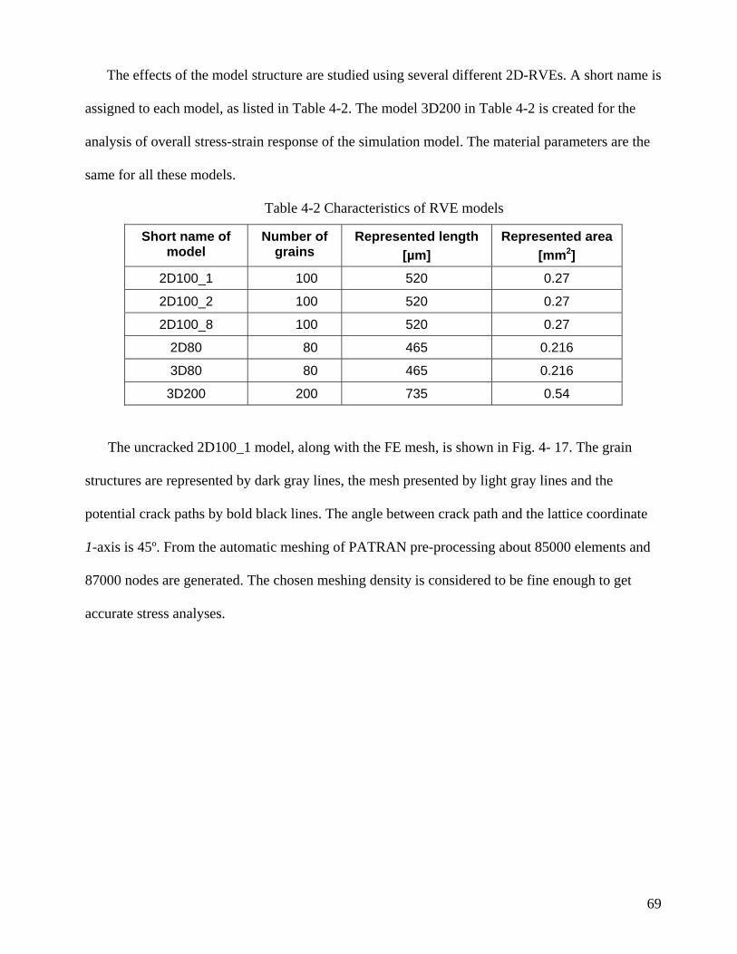
The effects of the model structure are studied using several different 2D-RVEs. A short name is
assigned to each model, as listed in Table 4-2. The model 3D200 in Table 4-2 is created for the
analysis of overall stress-strain response of the simulation model. The material parameters are the
same for all these models.
Table 4-2 Characteristics of RVE models
Short name of model
Number of grains
Represented length [µm]
Represented area [mm2]
2D100_1 100 520 0.27
2D100_2 100 520 0.27
2D100_8 100 520 0.27
2D80 80 465 0.216
3D80 80 465 0.216
3D200 200 735 0.54
The uncracked 2D100_1 model, along with the FE mesh, is shown in Fig. 4- 17. The grain
structures are represented by dark gray lines, the mesh presented by light gray lines and the
potential crack paths by bold black lines. The angle between crack path and the lattice coordinate
1-axis is 45º. From the automatic meshing of PATRAN pre-processing about 85000 elements and
87000 nodes are generated. The chosen meshing density is considered to be fine enough to get
accurate stress analyses.
69
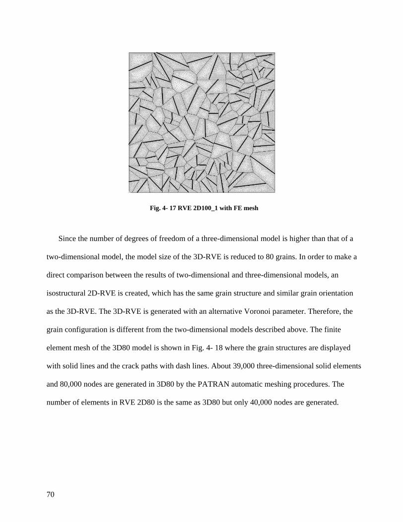
Fig. 4- 17 RVE 2D100_1 with FE mesh
Since the number of degrees of freedom of a three-dimensional model is higher than that of a
two-dimensional model, the model size of the 3D-RVE is reduced to 80 grains. In order to make a
direct comparison between the results of two-dimensional and three-dimensional models, an
isostructural 2D-RVE is created, which has the same grain structure and similar grain orientation
as the 3D-RVE. The 3D-RVE is generated with an alternative Voronoi parameter. Therefore, the
grain configuration is different from the two-dimensional models described above. The finite
element mesh of the 3D80 model is shown in Fig. 4- 18 where the grain structures are displayed
with solid lines and the crack paths with dash lines. About 39,000 three-dimensional solid elements
and 80,000 nodes are generated in 3D80 by the PATRAN automatic meshing procedures. The
number of elements in RVE 2D80 is the same as 3D80 but only 40,000 nodes are generated.
70
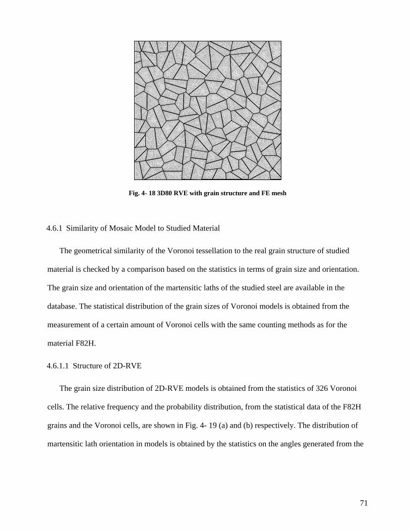
Fig. 4- 18 3D80 RVE with grain structure and FE mesh
4.6.1 Similarity of Mosaic Model to Studied Material
The geometrical similarity of the Voronoi tessellation to the real grain structure of studied
material is checked by a comparison based on the statistics in terms of grain size and orientation.
The grain size and orientation of the martensitic laths of the studied steel are available in the
database. The statistical distribution of the grain sizes of Voronoi models is obtained from the
measurement of a certain amount of Voronoi cells with the same counting methods as for the
material F82H.
4.6.1.1 Structure of 2D-RVE
The grain size distribution of 2D-RVE models is obtained from the statistics of 326 Voronoi
cells. The relative frequency and the probability distribution, from the statistical data of the F82H
grains and the Voronoi cells, are shown in Fig. 4- 19 (a) and (b) respectively. The distribution of
martensitic lath orientation in models is obtained by the statistics on the angles generated from the
71
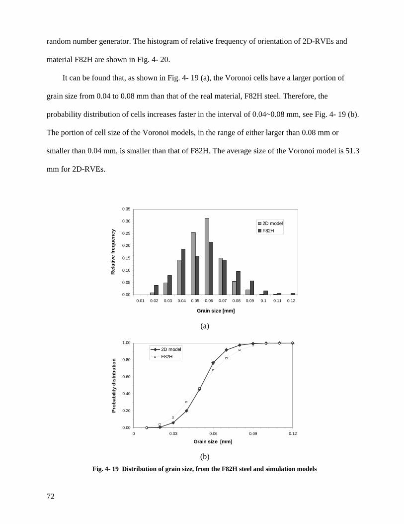
random number generator. The histogram of relative frequency of orientation of 2D-RVEs and
material F82H are shown in Fig. 4- 20.
It can be found that, as shown in Fig. 4- 19 (a), the Voronoi cells have a larger portion of
grain size from 0.04 to 0.08 mm than that of the real material, F82H steel. Therefore, the
probability distribution of cells increases faster in the interval of 0.04~0.08 mm, see Fig. 4- 19 (b).
The portion of cell size of the Voronoi models, in the range of either larger than 0.08 mm or
smaller than 0.04 mm, is smaller than that of F82H. The average size of the Voronoi model is 51.3
mm for 2D-RVEs.
0.00
0.05
0.10
0.15
0.20
0.25
0.30
0.35
0.01 0.02 0.03 0.04 0.05 0.06 0.07 0.08 0.09 0.1 0.11 0.12
Grain size [mm]
Rel
ativ
e fre
quen
cy
2D modelF82H
(a)
0.00
0.20
0.40
0.60
0.80
1.00
0 0.03 0.06 0.09 0.12
Grain size [mm]
Prob
abili
ty d
istri
butio
n
2D modelF82H
(b)
Fig. 4- 19 Distribution of grain size, from the F82H steel and simulation models
72
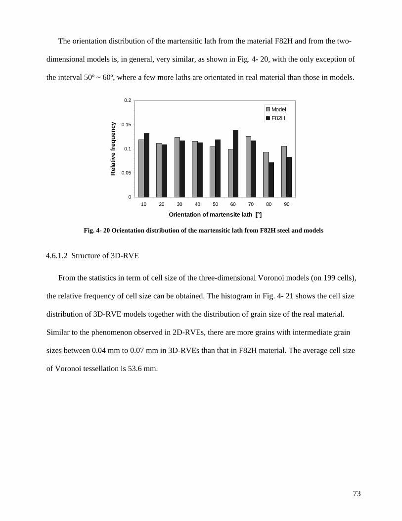
The orientation distribution of the martensitic lath from the material F82H and from the two-
dimensional models is, in general, very similar, as shown in Fig. 4- 20, with the only exception of
the interval 50º ~ 60º, where a few more laths are orientated in real material than those in models.
0
0.05
0.1
0.15
0.2
10 20 30 40 50 60 70 80 90
Orientation of martensite lath [°]
Rel
ativ
e fre
quen
cyModelF82H
Fig. 4- 20 Orientation distribution of the martensitic lath from F82H steel and models
4.6.1.2 Structure of 3D-RVE
From the statistics in term of cell size of the three-dimensional Voronoi models (on 199 cells),
the relative frequency of cell size can be obtained. The histogram in Fig. 4- 21 shows the cell size
distribution of 3D-RVE models together with the distribution of grain size of the real material.
Similar to the phenomenon observed in 2D-RVEs, there are more grains with intermediate grain
sizes between 0.04 mm to 0.07 mm in 3D-RVEs than that in F82H material. The average cell size
of Voronoi tessellation is 53.6 mm.
73
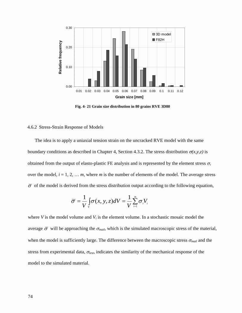
0.00
0.10
0.20
0.30
0.01 0.02 0.03 0.04 0.05 0.06 0.07 0.08 0.09 0.1 0.11 0.12
Grain size [mm]
Rel
ativ
e fre
quen
cy
3D modelF82H
Fig. 4- 21 Grain size distribution in 80 grains RVE 3D80
4.6.2 Stress-Strain Response of Models
The idea is to apply a uniaxial tension strain on the uncracked RVE model with the same
boundary conditions as described in Chapter 4, Section 4.3.2. The stress distribution σ(x,y,z) is
obtained from the output of elasto-plastic FE analysis and is represented by the element stress σι
over the model, i = 1, 2, … m, where m is the number of elements of the model. The average stress
σ of the model is derived from the stress distribution output according to the following equation,
∫ ∑=
==V
m
iiiVV
dVzyxV 1
1),,(1 σσσ
where V is the model volume and Vi is the element volume. In a stochastic mosaic model the
average σ will be approaching the σmatl, which is the simulated macroscopic stress of the material,
when the model is sufficiently large. The difference between the macroscopic stress σmatl and the
stress from experimental data, σtest, indicates the similarity of the mechanical response of the
model to the simulated material.
74
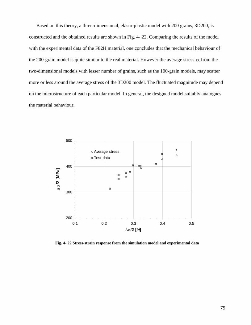
Based on this theory, a three-dimensional, elasto-plastic model with 200 grains, 3D200, is
constructed and the obtained results are shown in Fig. 4- 22. Comparing the results of the model
with the experimental data of the F82H material, one concludes that the mechanical behaviour of
the 200-grain model is quite similar to the real material. However the average stress σ from the
two-dimensional models with lesser number of grains, such as the 100-grain models, may scatter
more or less around the average stress of the 3D200 model. The fluctuated magnitude may depend
on the microstructure of each particular model. In general, the designed model suitably analogues
the material behaviour.
Fig. 4- 22 Stress-strain response from the simulation model and experimental data
200
300
400
500
0.1 0.2 0.3 0.4 0.5∆ε/2 [%]
∆σ
/2 [M
Pa]
Average stressTest data
75
CHAPTER 5 RESULTS OF 2D SIMULATIONS
The simulation results presented in this chapter are obtained from the following four kinds of
two-dimensional models: (1) plane-strain elastic model; (2) plane-stress elastic model; (3) plane-
strain elasto-plastic model and (4) plane-stress elasto-plastic model. The simulation is carried out
in two steps: at first tentatively assuming that the parameters in [41] are suitable to the studied
material and secondly correcting the simulation by using the optimum parameter(s) which will be
determined in the parameter study. The stress distributions obtained from finite element (FE)
analyses for the uncracked models are shown in Section 5.1. The crack density, i.e. the crack
number per unit area, is presented as the function of the number of cycles. The results of crack
density varying with the number of cycles obtained from simulation are presented in Section 5.2.
The method and results of parameter studies are also given in this section. In Section 5.3 the
stress redistribution caused by the introduced crack in the RVE and its influence on crack
initiation sequence are exhibited. In Section 5.4 crack patterns from elasto-plastic simulation are
presented.
To achieve a fast and efficient simulation, a program package is developed in the present
research, based on programs compiled at the University of Karlsruhe in a previous project. The
program package consists of some functional subroutines and even the ABAQUS code. It can
76
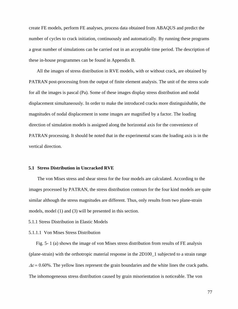
create FE models, perform FE analyses, process data obtained from ABAQUS and predict the
number of cycles to crack initiation, continuously and automatically. By running these programs
a great number of simulations can be carried out in an acceptable time period. The description of
these in-house programmes can be found in Appendix B.
All the images of stress distribution in RVE models, with or without crack, are obtained by
PATRAN post-processing from the output of finite element analysis. The unit of the stress scale
for all the images is pascal (Pa). Some of these images display stress distribution and nodal
displacement simultaneously. In order to make the introduced cracks more distinguishable, the
magnitudes of nodal displacement in some images are magnified by a factor. The loading
direction of simulation models is assigned along the horizontal axis for the convenience of
PATRAN processing. It should be noted that in the experimental scans the loading axis is in the
vertical direction.
5.1 Stress Distribution in Uncracked RVE
The von Mises stress and shear stress for the four models are calculated. According to the
images processed by PATRAN, the stress distribution contours for the four kind models are quite
similar although the stress magnitudes are different. Thus, only results from two plane-strain
models, model (1) and (3) will be presented in this section.
5.1.1 Stress Distribution in Elastic Models
5.1.1.1 Von Mises Stress Distribution
Fig. 5- 1 (a) shows the image of von Mises stress distribution from results of FE analysis
(plane-strain) with the orthotropic material response in the 2D100_1 subjected to a strain range
∆ε = 0.60%. The yellow lines represent the grain boundaries and the white lines the crack paths.
The inhomogeneous stress distribution caused by grain misorientation is noticeable. The von
77
Mises stress varies within each grain and from grain to grain. The difference between the highest
and the lowest value is about a factor of three.
A very impressive feature is the high stress concentration at triple-points and along the
neighbouring grain boundaries, as pointed out by arrows in Fig. 5- 1 (a). The stress concentration
at triple-points is a phenomenon often observed in experiments. One example is chosen in the
area inside frame A of Fig. 5- 1 (a), which is magnified and shown in Fig. 5- 1 (b). The highest
stress gradient occurs on the high-angle boundary of two adjacent grains, of which the orientation
difference is 42°. In general, the high stress gradient areas are found mostly near grain
boundaries.
The stress level and distribution within one grain is related to the orientation of the grain and
the misorientation of its neighbour grains. Some typical examples can be found in Fig. 5- 1 (c),
which is the magnified area within frame B in Fig. 5- 1 (a). The numbers in the blue boxes are
grain indexes. The grains numbered 12, 45 and 70 are oriented in the similar directions, which
can be recognized from their crack path orientations. The stress levels of these three grains are
similar, in the range from 400 MPa to 470 MPa. The grains numbered 61, 68 and 93, however,
undergo quite different stress levels, which vary from 340 MPa to 600 MPa in the elastic model,
although these grains are also similarly oriented. The highest stress levels occur in those grains,
where they are surrounded by the grains with the misorientation angle of about 45º. Two groups
of grains are selected for illustrating, for example, in Fig. 5- 1 (c) the grains numbered 58, 87 and
10 and the grains numbered 12, 70, 6, 45 and 90. The crack paths of grains numbered 58, 87 and
10 are oriented at about 0º or 90º. (Because of the symmetry of crystal bcc, the two grains with an
angle difference of 90º have the same orientations in the two-dimensional models.) The
orientations of crack path of grains numbered 12, 70, 6, 45 and 90 are all around ±45º to the
loading axis. Grains 10, 58 and 87 are surrounded by grains 12, 70, 6, 45 and 90. The von Mises
78
stress levels of the grains numbered 10, 58 and 87 (oriented ±45º to loading axis) are the highest
in the model.
The stress distribution contours under differently applied strain ranges are very similar in the
elastic analyses, but the stress amplitude is correspondingly higher if the applied strain range is
higher.
B
A
(a) Von Mises stress (Pa)
Loading direction
(b) Local area in square A of (a) (c) Local area in square B of (a)
Fig. 5- 1 Von Mises Stress distribution, 2D100_1, ∆ε = 0.60%, elastic model, PE
93
61
19
44
68
6
45
70
1058
90
12
87
Grain boundary
79
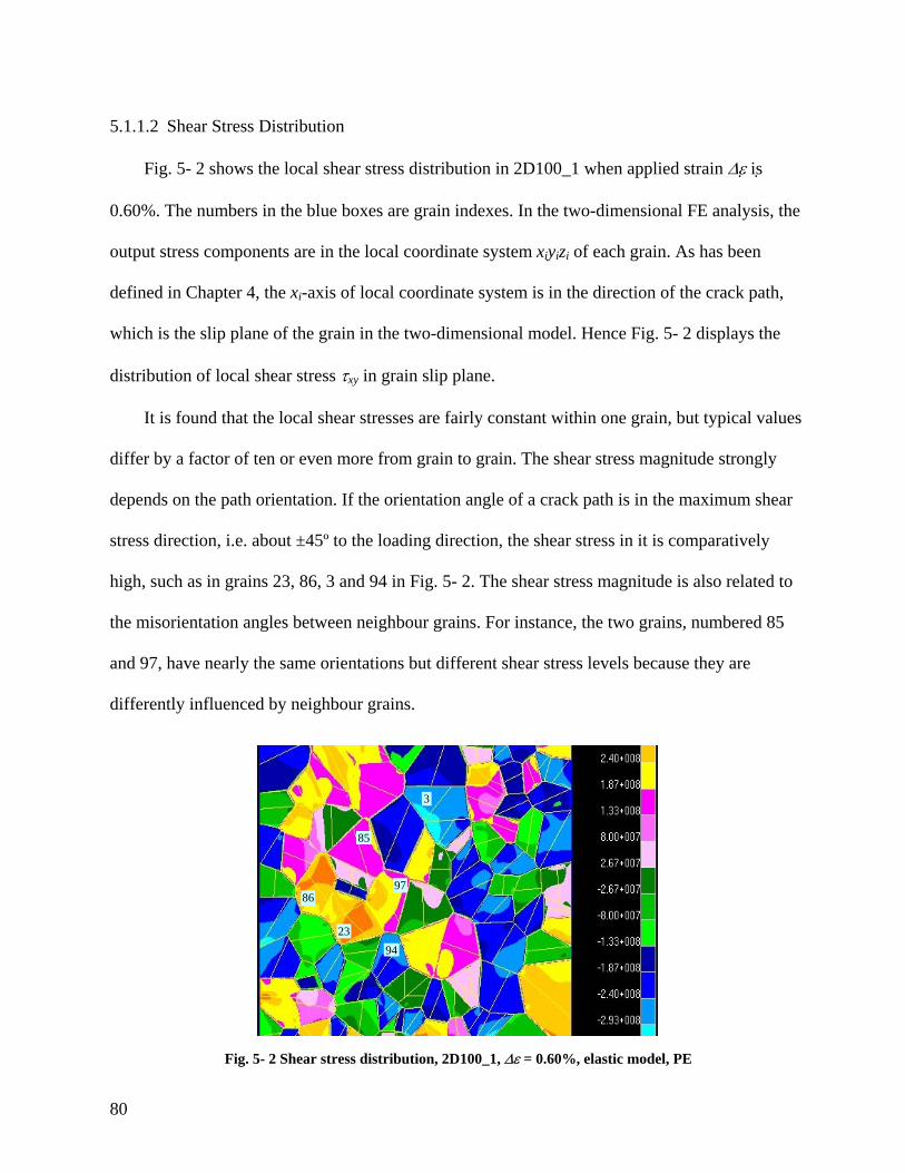
5.1.1.2 Shear Stress Distribution
Fig. 5- 2 shows the local shear stress distribution in 2D100_1 when applied strain ∆ε is
0.60%. The numbers in the blue boxes are grain indexes. In the two-dimensional FE analysis, the
output stress components are in the local coordinate system xiyizi of each grain. As has been
defined in Chapter 4, the xi-axis of local coordinate system is in the direction of the crack path,
which is the slip plane of the grain in the two-dimensional model. Hence Fig. 5- 2 displays the
distribution of local shear stress τxy in grain slip plane.
It is found that the local shear stresses are fairly constant within one grain, but typical values
differ by a factor of ten or even more from grain to grain. The shear stress magnitude strongly
depends on the path orientation. If the orientation angle of a crack path is in the maximum shear
stress direction, i.e. about ±45º to the loading direction, the shear stress in it is comparatively
high, such as in grains 23, 86, 3 and 94 in Fig. 5- 2. The shear stress magnitude is also related to
the misorientation angles between neighbour grains. For instance, the two grains, numbered 85
and 97, have nearly the same orientations but different shear stress levels because they are
differently influenced by neighbour grains.
85
97
3
23
86
94
Fig. 5- 2 Shear stress distribution, 2D100_1, ∆ε = 0.60%, elastic model, PE
80
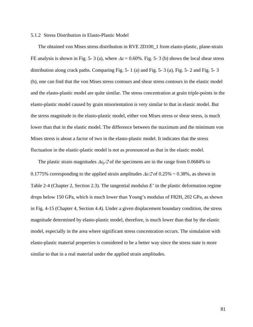
5.1.2 Stress Distribution in Elasto-Plastic Model
The obtained von Mises stress distribution in RVE 2D100_1 from elasto-plastic, plane-strain
FE analysis is shown in Fig. 5- 3 (a), where ∆ε = 0.60%. Fig. 5- 3 (b) shows the local shear stress
distribution along crack paths. Comparing Fig. 5- 1 (a) and Fig. 5- 3 (a), Fig. 5- 2 and Fig. 5- 3
(b), one can find that the von Mises stress contours and shear stress contours in the elastic model
and the elasto-plastic model are quite similar. The stress concentration at grain triple-points in the
elasto-plastic model caused by grain misorientation is very similar to that in elastic model. But
the stress magnitude in the elasto-plastic model, either von Mises stress or shear stress, is much
lower than that in the elastic model. The difference between the maximum and the minimum von
Mises stress is about a factor of two in the elasto-plastic model. It indicates that the stress
fluctuation in the elastic-plastic model is not as pronounced as that in the elastic model.
The plastic strain magnitudes ∆εp/2 of the specimens are in the range from 0.0684% to
0.1775% corresponding to the applied strain amplitudes ∆ε/2 of 0.25% ~ 0.38%, as shown in
Table 2-4 (Chapter 2, Section 2.3). The tangential modulus E’ in the plastic deformation regime
drops below 150 GPa, which is much lower than Young’s modulus of F82H, 202 GPa, as shown
in Fig. 4-15 (Chapter 4, Section 4.4). Under a given displacement boundary condition, the stress
magnitude determined by elasto-plastic model, therefore, is much lower than that by the elastic
model, especially in the area where significant stress concentration occurs. The simulation with
elasto-plastic material properties is considered to be a better way since the stress state is more
similar to that in a real material under the applied strain amplitudes.
81
(a) Von Mises stress (b) Local plastic shear strain Fig. 5- 3 Stress distribution, ∆ε = 0.60%, 2D100_1, elasto-plastic model, PE
5.2 Relations of Crack Density Versus Number of Cycles
The simulation yields the crack density Cd, i.e. the number of cracks per unit area, as the
function of the number of load cycles N, when the number of load cycles to crack initiation ∆N is
determined. The elastic model is not a suitable one for the stress analysis when a crack is
introduced into the model because it is not able to simulate the stress singularity at crack tips. The
stress magnitude determined by the elastic model is unreasonable high at crack tips, as will be
shown in the next section. Therefore only results from elasto-plastic models, under plane-strain
and plane-stress, are used for the quantitative analysis in this section.
5.2.1 Tentative Parameters
In elastic models, parameters G, Ws and τc in Eq. (4-8) are material constants. In the first step
of research, the tentative parameters from [41] for plain carbon steel, as listed in Table 5-1, were
applied. In the elasto-plastic models, the shear modulus G in Eq. (4-8) is no longer a constant in
the plastic deformation region. When the applied loading exceeds yield strength the shear
82
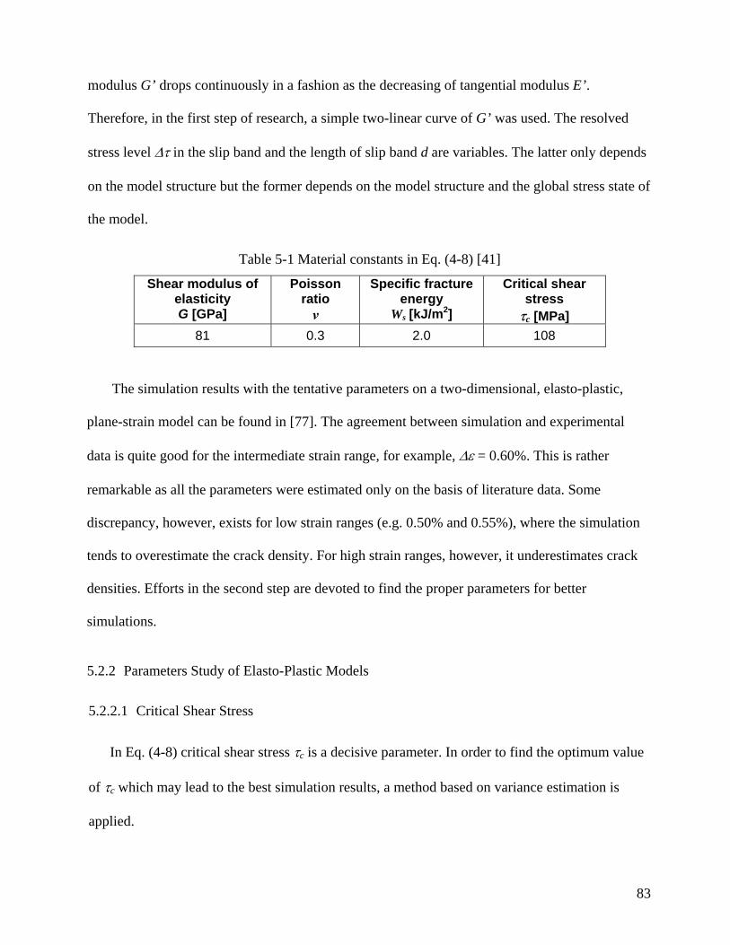
modulus G’ drops continuously in a fashion as the decreasing of tangential modulus E’.
Therefore, in the first step of research, a simple two-linear curve of G’ was used. The resolved
stress level ∆τ in the slip band and the length of slip band d are variables. The latter only depends
on the model structure but the former depends on the model structure and the global stress state of
the model.
Table 5-1 Material constants in Eq. (4-8) [41]
Shear modulus of elasticity G [GPa]
Poisson ratio ν
Specific fracture energy
Ws [kJ/m2]
Critical shear stress
τc [MPa] 81 0.3 2.0 108
The simulation results with the tentative parameters on a two-dimensional, elasto-plastic,
plane-strain model can be found in [77]. The agreement between simulation and experimental
data is quite good for the intermediate strain range, for example, ∆ε = 0.60%. This is rather
remarkable as all the parameters were estimated only on the basis of literature data. Some
discrepancy, however, exists for low strain ranges (e.g. 0.50% and 0.55%), where the simulation
tends to overestimate the crack density. For high strain ranges, however, it underestimates crack
densities. Efforts in the second step are devoted to find the proper parameters for better
simulations.
5.2.2 Parameters Study of Elasto-Plastic Models
5.2.2.1 Critical Shear Stress
In Eq. (4-8) critical shear stress τc is a decisive parameter. In order to find the optimum value
of τc which may lead to the best simulation results, a method based on variance estimation is
applied.
83
The idea is: A group of trial values, τc1, τc2,…τcM, are chosen and the two-dimensional
simulations are repeated with these trial values. For the ith strain range ∆ει and the jth value τcj, the
crack densities from simulation ijkdC )~( versus the numbers of cycles are calculated, i = 1, 2,
… n, j = 1, 2, … M, where n is the number of given strain ranges and M is the number of trial
values of τ
ijkN
cj. The subscript k corresponds to the crack density and the number of cycles at the kth
observation time, k = 1, 2, … ni, where ni is the number of observations. In this way the crack
density and the number of cycles N for all trial values of τdC~ cj under the applied strain ranges
∆ει can be obtained. The relation of from simulation results can be expressed by a power
function,
NCd −~
bij
ijd NAC )()~( = (5-1)
where A and b are fitting coefficients. From the curves, the variance between the
simulation results and the experimental data under the i
NCd −~ ijQ
th strain range can be calculated by
∑=
−=in
k
ijkd
ikdi
ij CC
nQ
1
2])~()[(1 (5-2)
where is the crack density of experimental data with respect to the kikdC )( th observation time.
One illustration is given in Fig. 5- 4.
The average variance jQ over all the strain ranges represents the degree of the
approximation of the simulation results to the experimental data of a trial τcj,
∑=
=n
i
ijj Q
nQ
1
1 (5-3)
By comparing the variances of all trial value of τcj, the minimum average value of variance minQ
can be found and the corresponding value of τcj is considered to be the optimum value of τc.
84
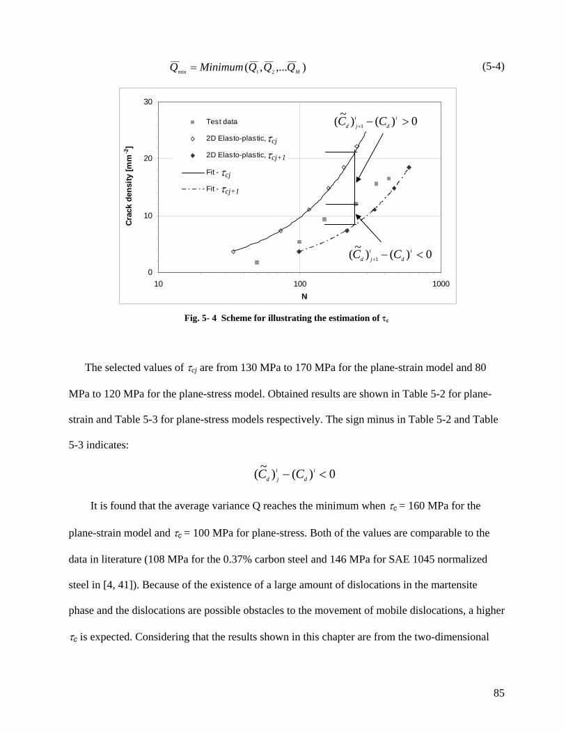
),...,( 21min MQQQMinimumQ = (5-4)
Fig. 5- 4 Scheme for illustrating the estimation of τc
The selected values of τcj are from 130 MPa to 170 MPa for the plane-strain model and 80
MPa to 120 MPa for the plane-stress model. Obtained results are shown in Table 5-2 for plane-
strain and Table 5-3 for plane-stress models respectively. The sign minus in Table 5-2 and Table
5-3 indicates:
0)()~( <− id
ijd CC
It is found that the average variance Q reaches the minimum when τc = 160 MPa for the
plane-strain model and τc = 100 MPa for plane-stress. Both of the values are comparable to the
data in literature (108 MPa for the 0.37% carbon steel and 146 MPa for SAE 1045 normalized
steel in [4, 41]). Because of the existence of a large amount of dislocations in the martensite
phase and the dislocations are possible obstacles to the movement of mobile dislocations, a higher
τc is expected. Considering that the results shown in this chapter are from the two-dimensional
0
10
20
30
10 100 1000N
Crac
k de
nsity
[mm
-2]
Test data
2D Elasto-plastic, 50
2D Elasto-plastic, 128
Fit - 5 0
Fit - 128
0)()~( 1 >−+i
dijd CC
0)()~( 1 <−+i
dijd CC
τcj+1
τcj
τcj+1
τcj
85
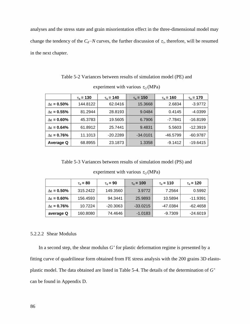
analyses and the stress state and grain misorientation effect in the three-dimensional model may
change the tendency of the Cd-N curves, the further discussion of τc, therefore, will be resumed
in the next chapter.
Table 5-2 Variances between results of simulation model (PE) and
experiment with various τcj (MPa)
τc = 130 τc = 140 τc = 150 τc = 160 τc = 170
∆ε = 0.50% 144.8122 62.0416 15.3668 2.6834 -3.9772
∆ε = 0.55% 81.2944 28.8193 9.0484 0.4145 -4.0399
∆ε = 0.60% 45.3783 19.5605 6.7906 -7.7841 -16.8199
∆ε = 0.64% 61.8912 25.7441 9.4831 5.5603 -12.3919
∆ε = 0.76% 11.1013 -20.2289 -34.0101 -46.5799 -60.9787
Average Q 68.8955 23.1873 1.3358 -9.1412 -19.6415
Table 5-3 Variances between results of simulation model (PS) and
experiment with various τcj (MPa)
τc = 80 τc = 90 τc = 100 τc = 110 τc = 120
∆ε = 0.50% 315.2422 149.3560 3.9772 7.2564 0.5992
∆ε = 0.60% 156.4593 94.3441 25.9893 10.5894 -11.9391
∆ε = 0.76% 10.7224 -20.3063 -33.0215 -47.0384 -62.4658
average Q 160.8080 74.4646 -1.0183 -9.7309 -24.6019
5.2.2.2 Shear Modulus
In a second step, the shear modulus G’ for plastic deformation regime is presented by a
fitting curve of quadrilinear form obtained from FE stress analysis with the 200 grains 3D elasto-
plastic model. The data obtained are listed in Table 5-4. The details of the determination of G’
can be found in Appendix D.
86
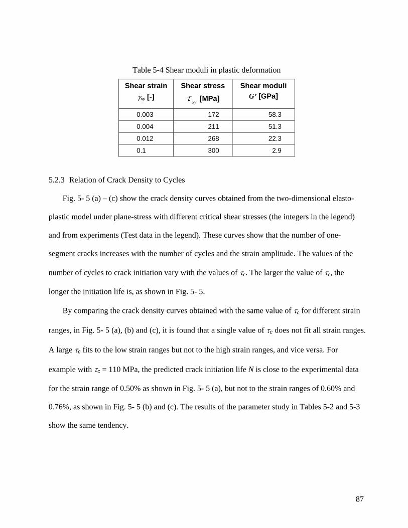
Table 5-4 Shear moduli in plastic deformation
Shear strain γxy [-]
Shear stress
xyτ [MPa]
Shear moduli G’ [GPa]
0.003 172 58.3
0.004 211 51.3
0.012 268 22.3
0.1 300 2.9
5.2.3 Relation of Crack Density to Cycles
Fig. 5- 5 (a) – (c) show the crack density curves obtained from the two-dimensional elasto-
plastic model under plane-stress with different critical shear stresses (the integers in the legend)
and from experiments (Test data in the legend). These curves show that the number of one-
segment cracks increases with the number of cycles and the strain amplitude. The values of the
number of cycles to crack initiation vary with the values of τc. The larger the value of τc, the
longer the initiation life is, as shown in Fig. 5- 5.
By comparing the crack density curves obtained with the same value of τc for different strain
ranges, in Fig. 5- 5 (a), (b) and (c), it is found that a single value of τc does not fit all strain ranges.
A large τc fits to the low strain ranges but not to the high strain ranges, and vice versa. For
example with τc = 110 MPa, the predicted crack initiation life N is close to the experimental data
for the strain range of 0.50% as shown in Fig. 5- 5 (a), but not to the strain ranges of 0.60% and
0.76%, as shown in Fig. 5- 5 (b) and (c). The results of the parameter study in Tables 5-2 and 5-3
show the same tendency.
87
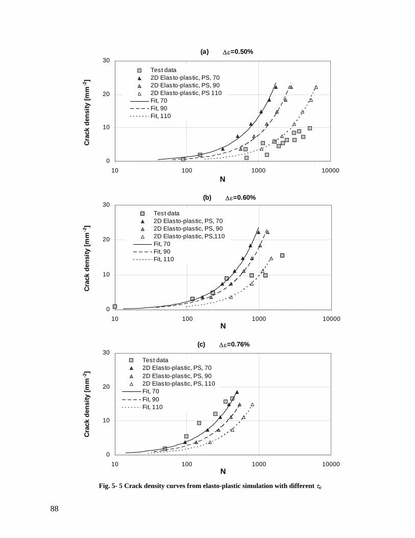
(a) ∆ε=0.50%
0
10
20
30
10 100 1000 10000N
Cra
ck d
ensi
ty [m
m-2
]
Test data2D Elasto-plastic, PS, 702D Elasto-plastic, PS, 902D Elasto-plastic, PS 110Fit, 70Fit, 90Fit, 110
(b) ∆ε=0.60%
0
10
20
30
10 100 1000 10000N
Cra
ck d
ensi
ty [m
m-2
]
Test data2D Elasto-plastic, PS, 702D Elasto-plastic, PS, 902D Elasto-plastic, PS,110Fit, 70Fit, 90Fit, 110
(c) ∆ε=0.76%
0
10
20
30
10 100 1000 10000N
Crac
k de
nsity
[mm
-2]
Test data2D Elasto-plastic, PS, 702D Elasto-plastic, PS, 902D Elasto-plastic, PS, 110Fit, 70Fit, 90Fit, 110
Fig. 5- 5 Crack density curves from elasto-plastic simulation with different τc
88
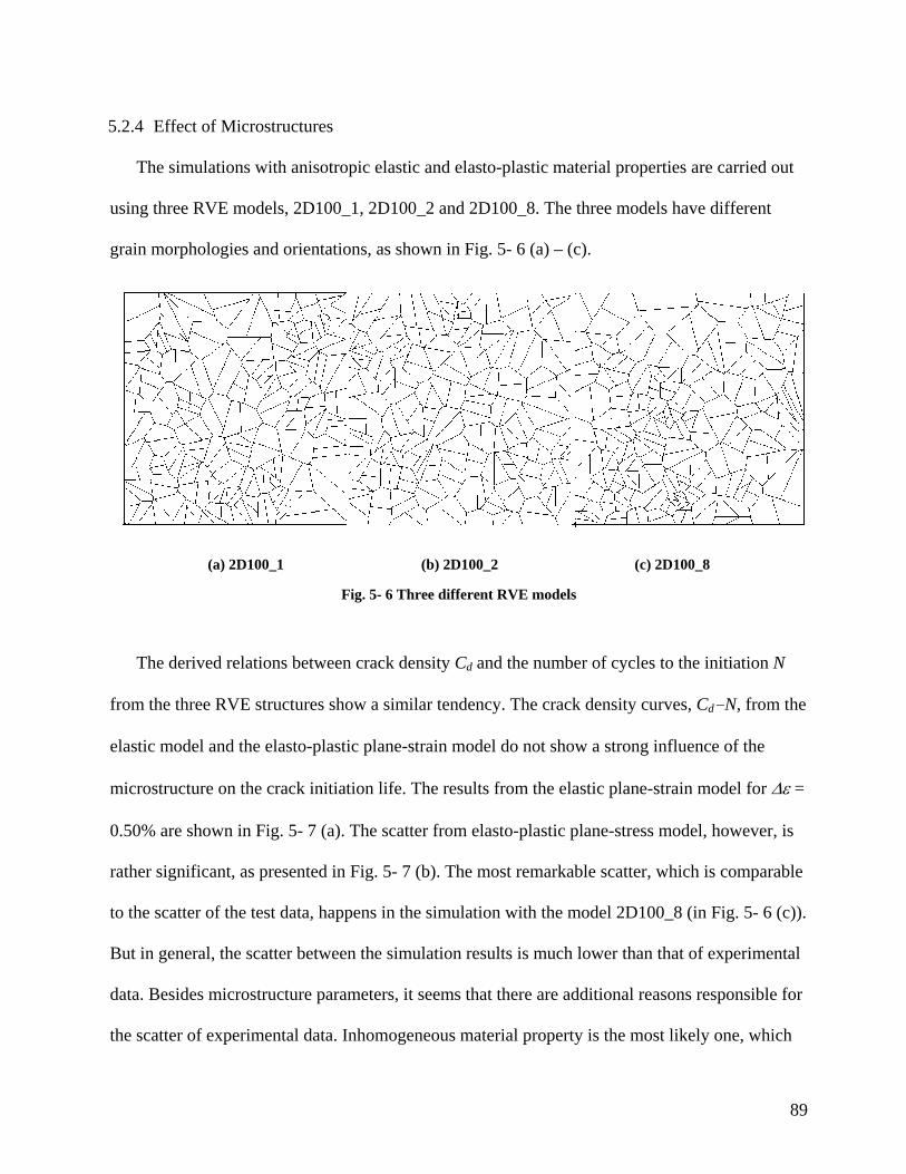
5.2.4 Effect of Microstructures
The simulations with anisotropic elastic and elasto-plastic material properties are carried out
using three RVE models, 2D100_1, 2D100_2 and 2D100_8. The three models have different
grain morphologies and orientations, as shown in Fig. 5- 6 (a) – (c).
(a) 2D100_1 (b) 2D100_2 (c) 2D100_8
Fig. 5- 6 Three different RVE models
The derived relations between crack density Cd and the number of cycles to the initiation N
from the three RVE structures show a similar tendency. The crack density curves, Cd-N, from the
elastic model and the elasto-plastic plane-strain model do not show a strong influence of the
microstructure on the crack initiation life. The results from the elastic plane-strain model for ∆ε =
0.50% are shown in Fig. 5- 7 (a). The scatter from elasto-plastic plane-stress model, however, is
rather significant, as presented in Fig. 5- 7 (b). The most remarkable scatter, which is comparable
to the scatter of the test data, happens in the simulation with the model 2D100_8 (in Fig. 5- 6 (c)).
But in general, the scatter between the simulation results is much lower than that of experimental
data. Besides microstructure parameters, it seems that there are additional reasons responsible for
the scatter of experimental data. Inhomogeneous material property is the most likely one, which
89
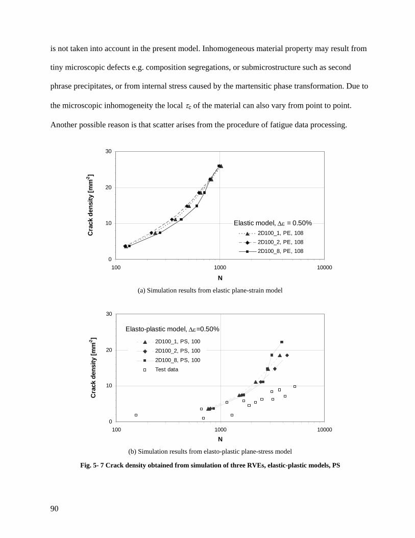
is not taken into account in the present model. Inhomogeneous material property may result from
tiny microscopic defects e.g. composition segregations, or submicrostructure such as second
phrase precipitates, or from internal stress caused by the martensitic phase transformation. Due to
the microscopic inhomogeneity the local τc of the material can also vary from point to point.
Another possible reason is that scatter arises from the procedure of fatigue data processing.
Elastic model, ∆ε = 0.50%
0
10
20
30
100 1000 10000
N
Cra
ck d
ensi
ty [m
m-2
]
2D100_1, PE, 1082D100_2, PE, 1082D100_8, PE, 108
(a) Simulation results from elastic plane-strain model
Elasto-plastic model, ∆ε=0.50%
0
10
20
30
100 1000 10000
N
Cra
ck d
ensi
ty [m
m-2
]
2D100_1, PS, 100
2D100_2, PS, 100
2D100_8, PS, 100
Test data
(b) Simulation results from elasto-plastic plane-stress model
Fig. 5- 7 Crack density obtained from simulation of three RVEs, elastic-plastic models, PS
90
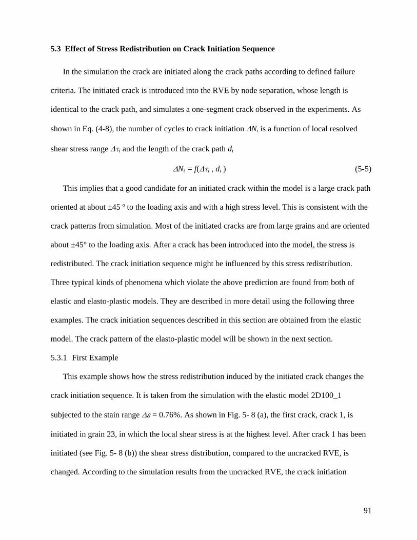
5.3 Effect of Stress Redistribution on Crack Initiation Sequence
In the simulation the crack are initiated along the crack paths according to defined failure
criteria. The initiated crack is introduced into the RVE by node separation, whose length is
identical to the crack path, and simulates a one-segment crack observed in the experiments. As
shown in Eq. (4-8), the number of cycles to crack initiation ∆Ni is a function of local resolved
shear stress range ∆τi and the length of the crack path di
∆Ni = f(∆τi , di ) (5-5)
This implies that a good candidate for an initiated crack within the model is a large crack path
oriented at about ±45 º to the loading axis and with a high stress level. This is consistent with the
crack patterns from simulation. Most of the initiated cracks are from large grains and are oriented
about ±45° to the loading axis. After a crack has been introduced into the model, the stress is
redistributed. The crack initiation sequence might be influenced by this stress redistribution.
Three typical kinds of phenomena which violate the above prediction are found from both of
elastic and elasto-plastic models. They are described in more detail using the following three
examples. The crack initiation sequences described in this section are obtained from the elastic
model. The crack pattern of the elasto-plastic model will be shown in the next section.
5.3.1 First Example
This example shows how the stress redistribution induced by the initiated crack changes the
crack initiation sequence. It is taken from the simulation with the elastic model 2D100_1
subjected to the stain range ∆ε = 0.76%. As shown in Fig. 5- 8 (a), the first crack, crack 1, is
initiated in grain 23, in which the local shear stress is at the highest level. After crack 1 has been
initiated (see Fig. 5- 8 (b)) the shear stress distribution, compared to the uncracked RVE, is
changed. According to the simulation results from the uncracked RVE, the crack initiation
91
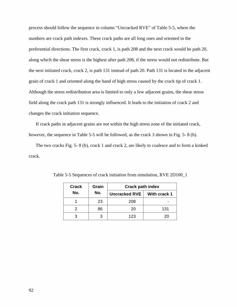
process should follow the sequence in column “Uncracked RVE” of Table 5-5, where the
numbers are crack path indexes. These crack paths are all long ones and oriented in the
preferential directions. The first crack, crack 1, is path 208 and the next crack would be path 20,
along which the shear stress is the highest after path 208, if the stress would not redistribute. But
the next initiated crack, crack 2, is path 131 instead of path 20. Path 131 is located in the adjacent
grain of crack 1 and oriented along the band of high stress caused by the crack tip of crack 1.
Although the stress redistribution area is limited to only a few adjacent grains, the shear stress
field along the crack path 131 is strongly influenced. It leads to the initiation of crack 2 and
changes the crack initiation sequence.
If crack paths in adjacent grains are not within the high stress zone of the initiated crack,
however, the sequence in Table 5-5 will be followed, as the crack 3 shown in Fig. 5- 8 (b).
The two cracks Fig. 5- 8 (b), crack 1 and crack 2, are likely to coalesce and to form a kinked
crack.
Table 5-5 Sequences of crack initiation from simulation, RVE 2D100_1
Crack path index Crack No.
Grain No. Uncracked RVE With crack 1
1 23 208 -
2 86 20 131
3 3 123 20
92
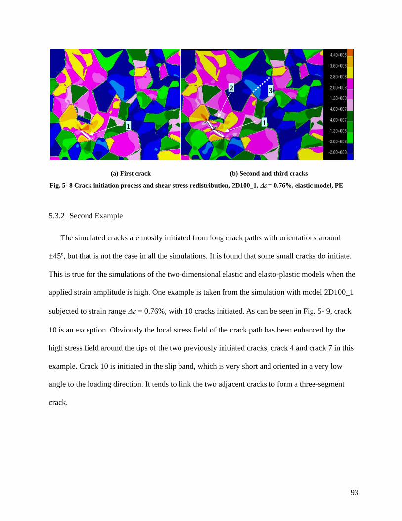
(a) First crack (b) Second and third cracks
Fig. 5- 8 Crack initiation process and shear stress redistribution, 2D100_1, ∆ε = 0.76%, elastic model, PE
1
2
1
3
5.3.2 Second Example
The simulated cracks are mostly initiated from long crack paths with orientations around
±45º, but that is not the case in all the simulations. It is found that some small cracks do initiate.
This is true for the simulations of the two-dimensional elastic and elasto-plastic models when the
applied strain amplitude is high. One example is taken from the simulation with model 2D100_1
subjected to strain range ∆ε = 0.76%, with 10 cracks initiated. As can be seen in Fig. 5- 9, crack
10 is an exception. Obviously the local stress field of the crack path has been enhanced by the
high stress field around the tips of the two previously initiated cracks, crack 4 and crack 7 in this
example. Crack 10 is initiated in the slip band, which is very short and oriented in a very low
angle to the loading direction. It tends to link the two adjacent cracks to form a three-segment
crack.
93
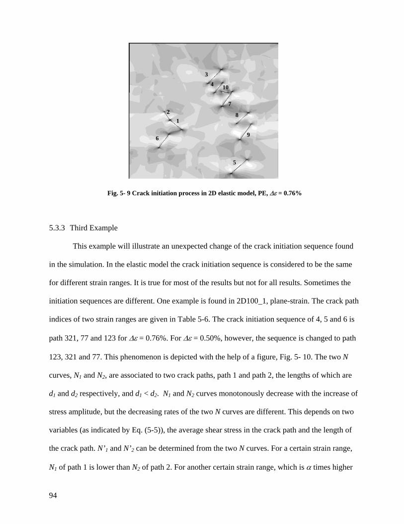
10
9
8
7
6
5
4
3
2 1
Fig. 5- 9 Crack initiation process in 2D elastic model, PE, ∆ε = 0.76%
5.3.3 Third Example
This example will illustrate an unexpected change of the crack initiation sequence found
in the simulation. In the elastic model the crack initiation sequence is considered to be the same
for different strain ranges. It is true for most of the results but not for all results. Sometimes the
initiation sequences are different. One example is found in 2D100_1, plane-strain. The crack path
indices of two strain ranges are given in Table 5-6. The crack initiation sequence of 4, 5 and 6 is
path 321, 77 and 123 for ∆ε = 0.76%. For ∆ε = 0.50%, however, the sequence is changed to path
123, 321 and 77. This phenomenon is depicted with the help of a figure, Fig. 5- 10. The two N
curves, N1 and N2, are associated to two crack paths, path 1 and path 2, the lengths of which are
d1 and d2 respectively, and d1 < d2. N1 and N2 curves monotonously decrease with the increase of
stress amplitude, but the decreasing rates of the two N curves are different. This depends on two
variables (as indicated by Eq. (5-5)), the average shear stress in the crack path and the length of
the crack path. N’1 and N’2 can be determined from the two N curves. For a certain strain range,
N1 of path 1 is lower than N2 of path 2. For another certain strain range, which is α times higher
94
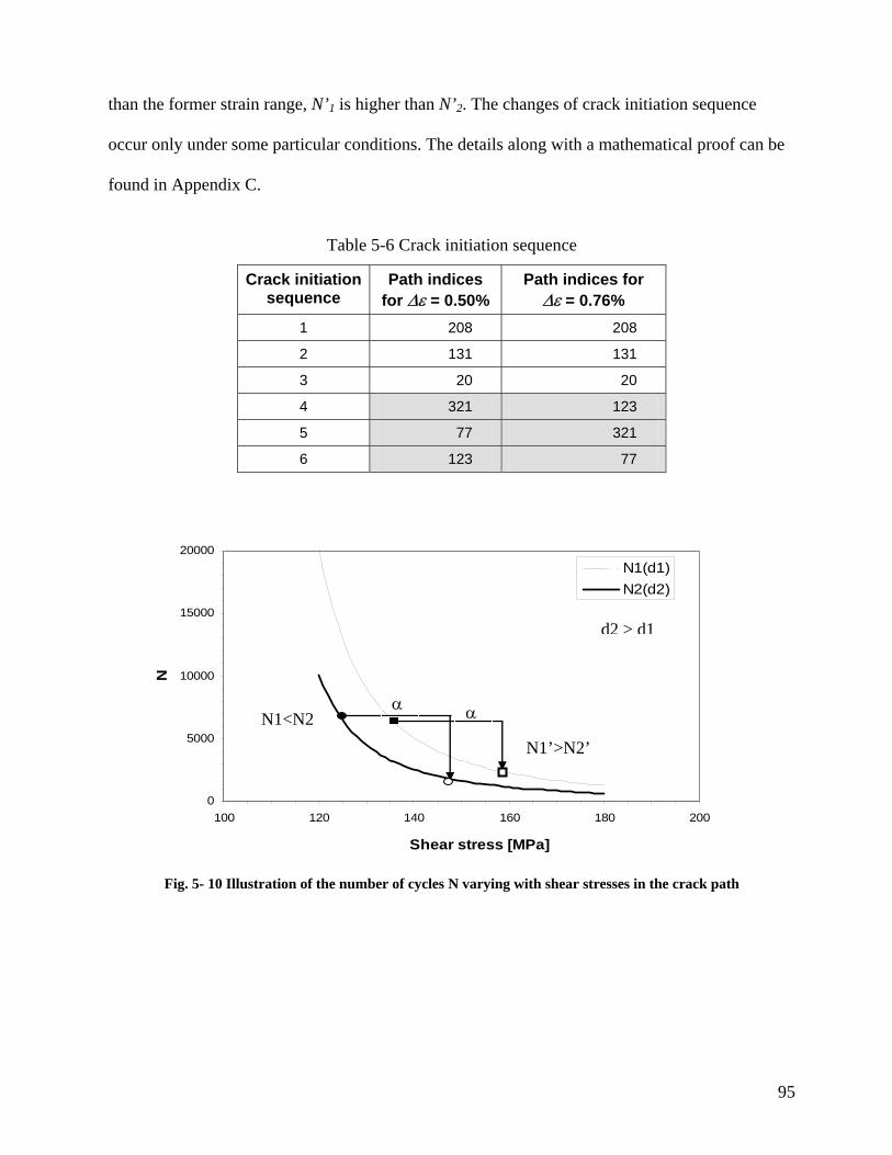
than the former strain range, N’1 is higher than N’2. The changes of crack initiation sequence
occur only under some particular conditions. The details along with a mathematical proof can be
found in Appendix C.
Table 5-6 Crack initiation sequence
Crack initiation sequence
Path indices for ∆ε = 0.50%
Path indices for ∆ε = 0.76%
1 208 208
2 131 131
3 20 20
4 321 123
5 77 321
6 123 77
Fig. 5- 10 Illustration of the number of cycles N varying with shear stresses in the crack path
0
5000
10000
15000
20000
100 120 140 160 180 200
Shear stress [MPa]
N
N1(d1)N2(d2)
d2 > d1
α α
N1’>N2’
N1<N2
95
5.4 Crack Patterns of Elasto-Plastic Model
Fig. 5- 11 (a) – (c) show the simulated crack initiation process with the elasto-plastic model
2D100_1 for ∆ε = 0.50%. No interaction between the microcracks is visible at the beginning of
the process. As the simulation progresses, two crack clusters consisting of several interacting
cracks are formed, whereas extended interacting plastic zones can also be observed. In this way
cracks within one cluster are likely to form a macrocrack by coalescence. Eventually a long
macro-crack will be formed by cluster coalescence.
A typical feature in the high strain range (∆ε = 0.76%) is that crack strata are formed, i.e.
there are bands with cracks and undamaged regions; the cracks tend to arrange themselves in
parallel stacks within one crack strata, as shown in Fig. 5- 12. High plastic strains are observed
between the cracks and the plastic zones of neighbouring cracks interact. If a crack path is located
in the high stress zone, a low angle crack may initiate, such as crack 9 shown in Fig. 5- 9, which
lies between two initiated cracks (crack 4 and 5). This indicates that a long zigzag crack will be
formed by coalescence and a simulation based solely on crack initiation does not seem to be
realistic beyond this point.
The typical crack pattern observed in the experiment at a medium strain range is shown in
Fig. 5- 13. Arrows point to microcracks. It can be concluded that the characteristic features
described above are also visible in the experiment.
96
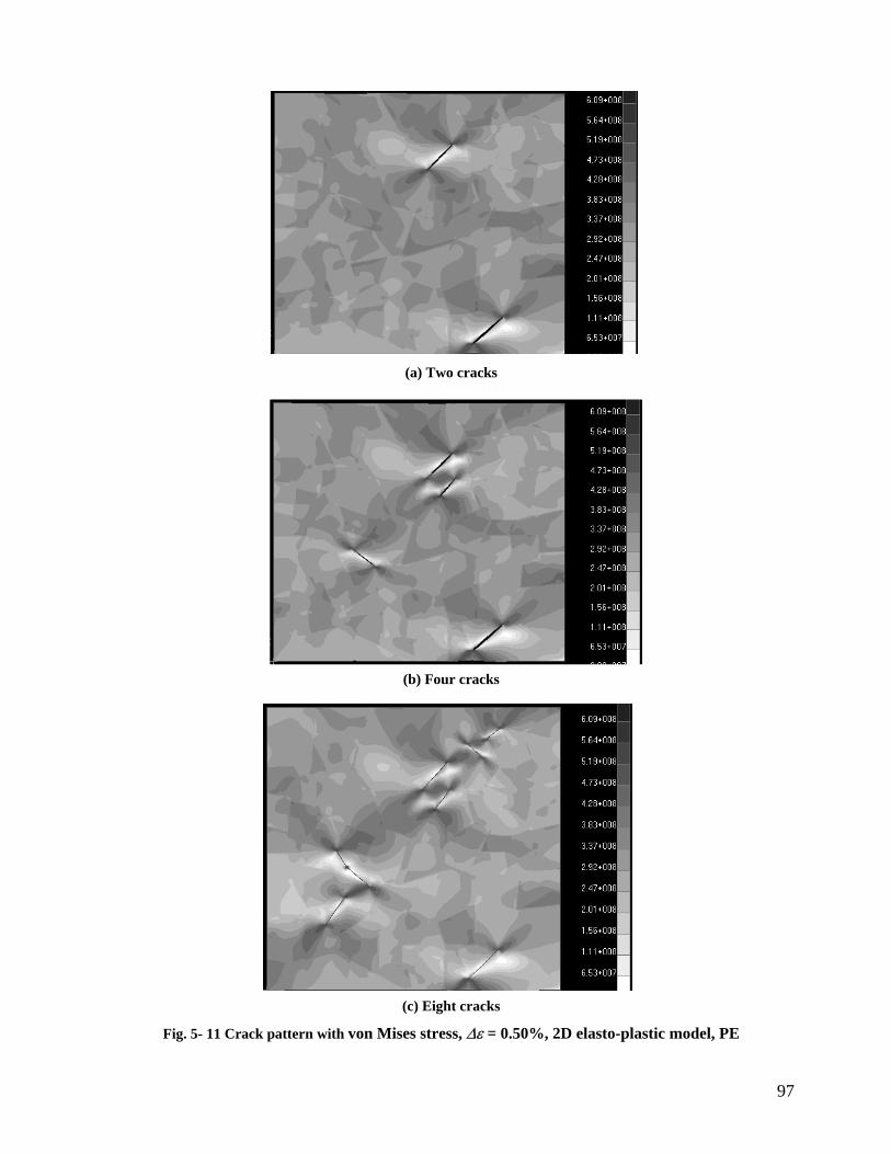
(a) Two cracks
(b) Four cracks
(c) Eight cracks
Fig. 5- 11 Crack pattern with von Mises stress, ∆ε = 0.50%, 2D elasto-plastic model, PE
97
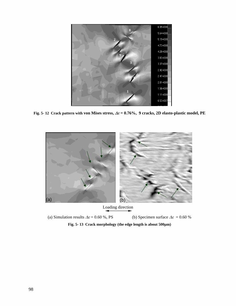
Fig. 5- 12 Crack pattern with von Mises stress, ∆ε = 0.76%, 9 cracks, 2D elasto-plastic model, PE
(a) Simulation results ∆ε = 0.60 %, PS (b) Specimen surface ∆ε = 0.60 %
Fig. 5- 13 Crack morphology (the edge length is about 500µm)
9
8
7
6
5
4 3
2
1
(a) (b)Loading direction
98
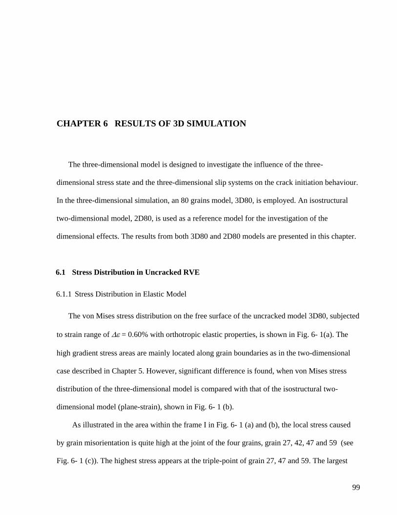
CHAPTER 6 RESULTS OF 3D SIMULATION
The three-dimensional model is designed to investigate the influence of the three-
dimensional stress state and the three-dimensional slip systems on the crack initiation behaviour.
In the three-dimensional simulation, an 80 grains model, 3D80, is employed. An isostructural
two-dimensional model, 2D80, is used as a reference model for the investigation of the
dimensional effects. The results from both 3D80 and 2D80 models are presented in this chapter.
6.1 Stress Distribution in Uncracked RVE
6.1.1 Stress Distribution in Elastic Model
The von Mises stress distribution on the free surface of the uncracked model 3D80, subjected
to strain range of ∆ε = 0.60% with orthotropic elastic properties, is shown in Fig. 6- 1(a). The
high gradient stress areas are mainly located along grain boundaries as in the two-dimensional
case described in Chapter 5. However, significant difference is found, when von Mises stress
distribution of the three-dimensional model is compared with that of the isostructural two-
dimensional model (plane-strain), shown in Fig. 6- 1 (b).
As illustrated in the area within the frame I in Fig. 6- 1 (a) and (b), the local stress caused
by grain misorientation is quite high at the joint of the four grains, grain 27, 42, 47 and 59 (see
Fig. 6- 1 (c)). The highest stress appears at the triple-point of grain 27, 47 and 59. The largest
99
mismatch angle is 52° between grains 47 and 59 in XY-plane. In the two-dimensional model,
however, the stress level at the same point is not as high as that in the three-dimensional model.
Another example is at a grain triple-point in the area within the frame II in Fig. 6- 1 (a) and
(b). The von Mises stress distribution in the three grains, grain 14, 40 and 65, is shown in Fig. 6-
1 (d). The grain misorientation between grain 40 and grain 65 is 34° whereas the grain boundary
of grain 14 and 65 is a low angle boundary. At this point the stress level in the two-dimensional
model is higher than that in the three-dimensional model.
It is found that the influencing factor for the above two samples is the same, i.e. the grain
orientation in the depth. For the first example, the mismatch angle in depth is 52° and for the
second it is about 10°. Therefore, the stress levels at these two places are altered in different
ways: In the first example it is enhanced and in the second example it is weakened by the grain
misorientation in the third dimension.
Because the local coordinate systems in the three-dimensional model are not set in the
directions of crack paths along the slip directions, the local shear stress along the slip plane
cannot be directly displayed.
6.1.2 Stress Distribution in Elasto-Plastic Model
Fig. 6- 2 (a)-(c) exhibit the von Mises stress with grain structure in the uncracked three-
dimensional elasto-plastic model (Fig. 6- 2 (a)), the two-dimensional plane-stress model (Fig. 6-
2 (b)) and plane-strain model (Fig. 6- 2 (c)). The applied strain ∆ε is 0.60%. The difference of
the von Mises stress distribution between the 2D and 3D elasto-plastic models is considerable.
The magnitude of inhomogeneous stress seems higher in the 2D plane-strain model. The effect
of grain misorientation in depth between the elasto-plastic 3D and 2D plane-strain model is
similar to that between the corresponding elastic models. The overall stress level of the 3D
100
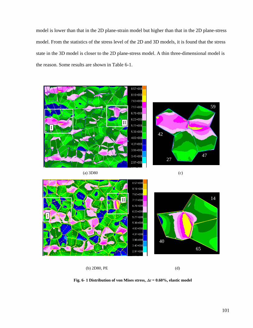
model is lower than that in the 2D plane-strain model but higher than that in the 2D plane-stress
model. From the statistics of the stress level of the 2D and 3D models, it is found that the stress
state in the 3D model is closer to the 2D plane-stress model. A thin three-dimensional model is
the reason. Some results are shown in Table 6-1.
(a) 3D80 (c)
(b) 2D80, PE (d)
Fig. 6- 1 Distribution of von Mises stress, ∆ε = 0.60%, elastic model
III
42
47
59
27
I
II
65
14
40
101
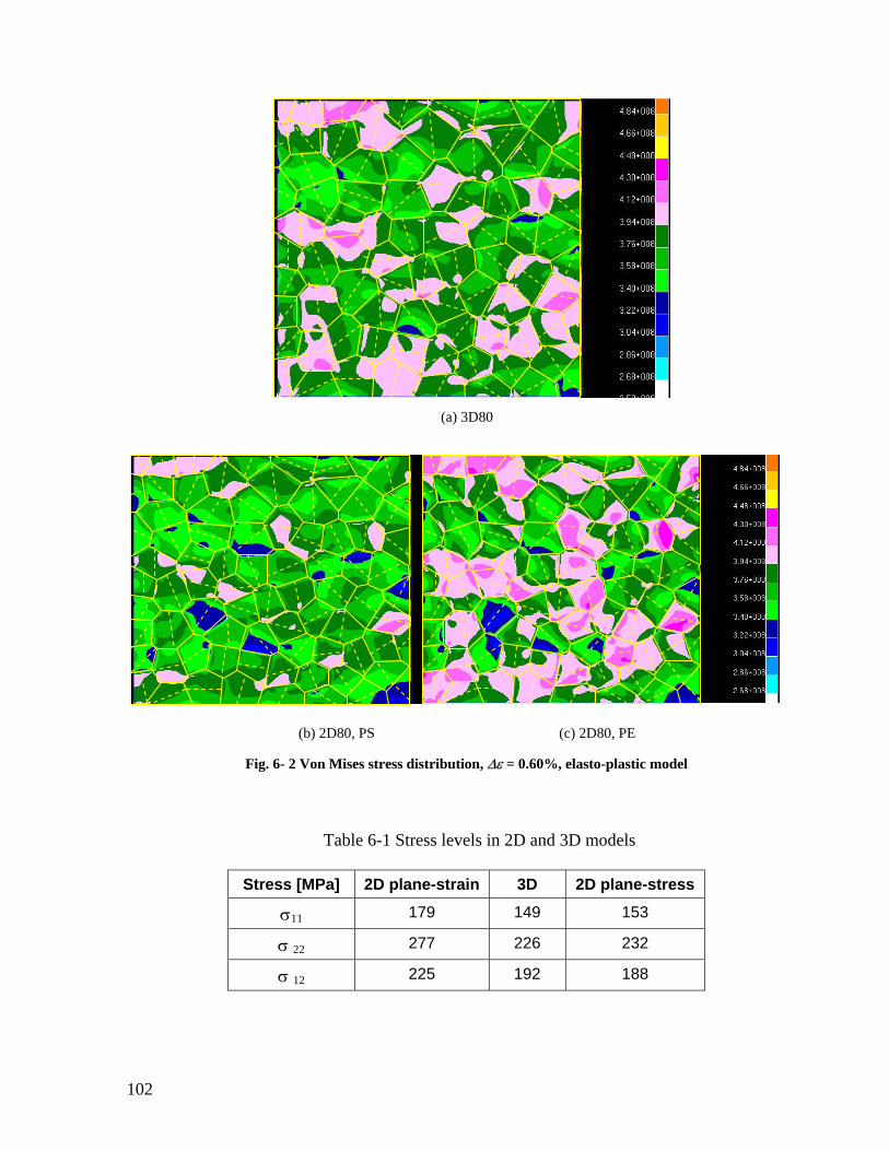
(a) 3D80
(b) 2D80, PS (c) 2D80, PE
Fig. 6- 2 Von Mises stress distribution, ∆ε = 0.60%, elasto-plastic model
Table 6-1 Stress levels in 2D and 3D models
Stress [MPa] 2D plane-strain 3D 2D plane-stress
σ11 179 149 153
σ 22 277 226 232
σ 12 225 192 188
102
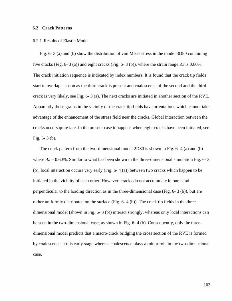
6.2 Crack Patterns
6.2.1 Results of Elastic Model
Fig. 6- 3 (a) and (b) show the distribution of von Mises stress in the model 3D80 containing
five cracks (Fig. 6- 3 (a)) and eight cracks (Fig. 6- 3 (b)), where the strain range ∆ε is 0.60%.
The crack initiation sequence is indicated by index numbers. It is found that the crack tip fields
start to overlap as soon as the third crack is present and coalescence of the second and the third
crack is very likely, see Fig. 6- 3 (a). The next cracks are initiated in another section of the RVE.
Apparently those grains in the vicinity of the crack tip fields have orientations which cannot take
advantage of the enhancement of the stress field near the cracks. Global interaction between the
cracks occurs quite late. In the present case it happens when eight cracks have been initiated, see
Fig. 6- 3 (b).
The crack pattern from the two-dimensional model 2D80 is shown in Fig. 6- 4 (a) and (b)
where ∆ε = 0.60%. Similar to what has been shown in the three-dimensional simulation Fig. 6- 3
(b), local interaction occurs very early (Fig. 6- 4 (a)) between two cracks which happen to be
initiated in the vicinity of each other. However, cracks do not accumulate in one band
perpendicular to the loading direction as in the three-dimensional case (Fig. 6- 3 (b)), but are
rather uniformly distributed on the surface (Fig. 6- 4 (b)). The crack tip fields in the three-
dimensional model (shown in Fig. 6- 3 (b)) interact strongly, whereas only local interactions can
be seen in the two-dimensional case, as shown in Fig. 6- 4 (b). Consequently, only the three-
dimensional model predicts that a macro-crack bridging the cross section of the RVE is formed
by coalescence at this early stage whereas coalescence plays a minor role in the two-dimensional
case.
103
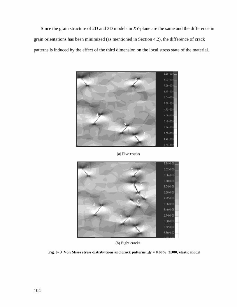
Since the grain structure of 2D and 3D models in XY-plane are the same and the difference in
grain orientations has been minimized (as mentioned in Section 4.2), the difference of crack
patterns is induced by the effect of the third dimension on the local stress state of the material.
(a) Five cracks
(b) Eight cracks
Fig. 6- 3 Von Mises stress distributions and crack patterns, ∆ε = 0.60%, 3D80, elastic model
5
4
3
2
1
8 7
6
5
4
3
2
1
104
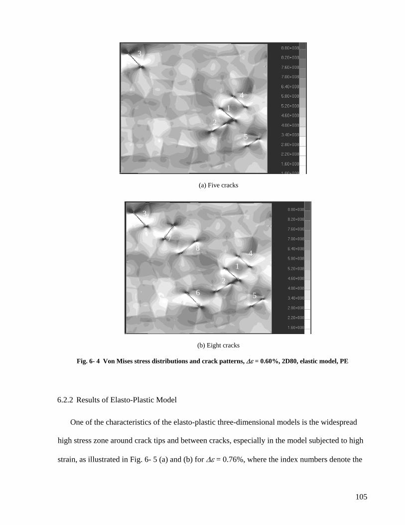
(a) Five cracks
(b) Eight cracks
Fig. 6- 4 Von Mises stress distributions and crack patterns, ∆ε = 0.60%, 2D80, elastic model, PE
2
1
5
4
3
7
2
1
6 5
4 8
3
6.2.2 Results of Elasto-Plastic Model
One of the characteristics of the elasto-plastic three-dimensional models is the widespread
high stress zone around crack tips and between cracks, especially in the model subjected to high
strain, as illustrated in Fig. 6- 5 (a) and (b) for ∆ε = 0.76%, where the index numbers denote the
105

crack initiation sequence. In Fig. 6- 5 (a), two high stress areas are visible, one between crack 1
and 3 and the other between crack 3 and 4. Some cracks are initiated inside these high stress
areas, for example cracks 5, 6 and 7. The patterns from simulation with elasto-plastic model
show very intensive crack interaction, as shown in Fig. 6- 5 (b).
As in the two-dimensional model, a low angle crack, crack 9, initiates between two initiated
cracks, cracks 5 and 8, see Fig. 6- 5 (b). Crack coalescence is likely between crack 3, 5, 9, 8 and
10 leading to a zigzag crack, which is possibly one part of a macrocrack.
(a) Four cracks
(b) Eleven cracks
Fig. 6- 5 Crack initiation sequence, 3D80, ∆ε = 0.76%, elasto-plastic model
1
3
4
2
2
1
4
3
9
10
7
2
1
6
5
4
8
3
106
6.3 Relations of Crack Density to Number of Cycles
In this section, the relations of the crack density versus the number of cycles, i.e. the Cd-N
curves, are determined by two equations, the Tanaka-Mura equation and the Chan equation, with
both of the two-dimensional and the three dimensional models. For the two-dimensional models,
the simulation is conducted either in a plane-strain or plane-stress state.
6.3.1 Results from Tanaka-Mura Equation
The simulations are carried out with the tentative parameters (Table 5-2, Chapter 5, Section
5.3) and elastic and elasto-plastic properties. Fig. 6- 6 shows the Cd-N curves obtained from
elastic models and Fig. 6- 7 shows the results obtained from elasto-plastic models. For the sake
of comparison, the crack density curves obtained from the two-dimensional plane-stress (PS) and
plane-strain (PE), along with the three-dimensional models, are presented in one diagram. As
shown in Fig. 6- 6 and Fig. 6- 7, it is found that for both elastic and elasto-plastic material
properties, the Cd-N curve of the three-dimensional model lies between the curves of the two-
dimensional plane-strain and plane-stress models. Since the structures of the two-dimensional
and three-dimensional models are almost the same, the difference should not be caused by the
microstructure. The parameters in the Tanaka-Mura equation and constants of the material
property are the same for all the models. The reason of the difference between 2D and 3D
models is attributed to the stress state. As has been analyzed in section 6.1, the overall stress
level of the 3D model is lower than that in the two-dimensional plane-strain model but higher
than that in the plane-stress model. The Cd-N curves of the 2D and 3D models show the same
tendency. The crack density determined by the three-dimensional simulation increases faster
than that determined by the two-dimensional plane-stress model but slower than that by the two-
dimensional plane-strain model. In other words, the results show the stress state dependence.
107
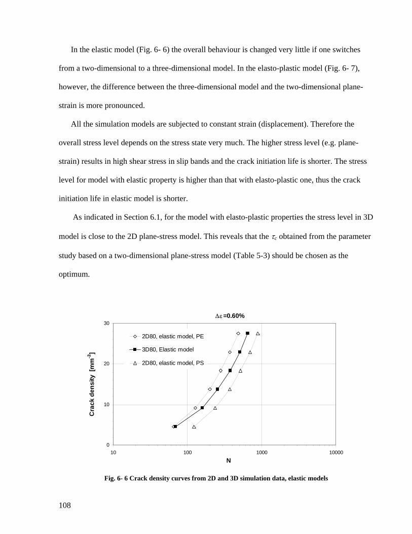
In the elastic model (Fig. 6- 6) the overall behaviour is changed very little if one switches
from a two-dimensional to a three-dimensional model. In the elasto-plastic model (Fig. 6- 7),
however, the difference between the three-dimensional model and the two-dimensional plane-
strain is more pronounced.
All the simulation models are subjected to constant strain (displacement). Therefore the
overall stress level depends on the stress state very much. The higher stress level (e.g. plane-
strain) results in high shear stress in slip bands and the crack initiation life is shorter. The stress
level for model with elastic property is higher than that with elasto-plastic one, thus the crack
initiation life in elastic model is shorter.
As indicated in Section 6.1, for the model with elasto-plastic properties the stress level in 3D
model is close to the 2D plane-stress model. This reveals that the τc obtained from the parameter
study based on a two-dimensional plane-stress model (Table 5-3) should be chosen as the
optimum.
∆ε=0.60%
0
10
20
30
10 100 1000 10000N
Cra
ck d
ensi
ty [
mm
-2]
2D80, elastic model, PE
3D80, Elastic model
2D80, elastic model, PS
Fig. 6- 6 Crack density curves from 2D and 3D simulation data, elastic models
108
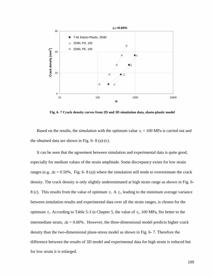
∆ε=0.60%
0
10
20
30
10 100 1000 10000N
Cra
ck d
ensi
ty [m
m-2
]
T-M, Elasto-Plastic, 3D80
2D80, PS, 100
2D80, PE, 100
Fig. 6- 7 Crack density curves from 2D and 3D simulation data, elasto-plastic model
Based on the results, the simulation with the optimum value τc = 100 MPa is carried out and
the obtained data are shown in Fig. 6- 8 (a)-(c).
It can be seen that the agreement between simulation and experimental data is quite good,
especially for medium values of the strain amplitude. Some discrepancy exists for low strain
ranges (e.g. ∆ε = 0.50%, Fig. 6- 8 (a)) where the simulation still tends to overestimate the crack
density. The crack density is only slightly underestimated at high strain range as shown in Fig. 6-
8 (c). This results from the value of optimum τc. A τc, leading to the minimum average variance
between simulation results and experimental data over all the strain ranges, is chosen for the
optimum τc. According to Table 5-3 in Chapter 5, the value of τc, 100 MPa, fits better to the
intermediate strain, ∆ε = 0.60%. However, the three-dimensional model predicts higher crack
density than the two-dimensional plane-stress model as shown in Fig. 6- 7. Therefore the
difference between the results of 3D model and experimental data for high strain is reduced but
for low strain it is enlarged.
109
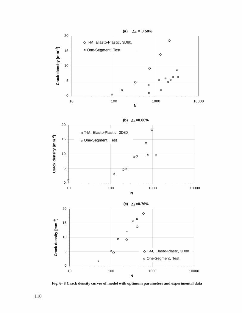
(a) ∆ε = 0.50%
0
5
10
15
20
10 100 1000 10000N
Crac
k de
nsity
[mm
-2]
T-M, Elasto-Plastic, 3D80,
One-Segment, Test
(b) ∆ε=0.60%
0
5
10
15
20
10 100 1000 10000N
Crac
k de
nsity
[mm
-2] T-M, Elasto-Plastic, 3D80
One-Segment, Test
(c) ∆ε=0.76%
0
5
10
15
20
10 100 1000 10000N
Crac
k de
nsity
[mm
-2]
T-M, Elasto-Plastc, 3D80
One-Segment, Test
Fig. 6- 8 Crack density curves of model with optimum parameters and experimental data
110
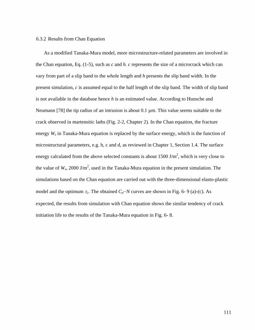
6.3.2 Results from Chan Equation
As a modified Tanaka-Mura model, more microstructure-related parameters are involved in
the Chan equation, Eq. (1-5), such as c and h. c represents the size of a microcrack which can
vary from part of a slip band to the whole length and h presents the slip band width. In the
present simulation, c is assumed equal to the half length of the slip band. The width of slip band
is not available in the database hence h is an estimated value. According to Hunsche and
Neumann [78] the tip radius of an intrusion is about 0.1 µm. This value seems suitable to the
crack observed in martensitic laths (Fig. 2-2, Chapter 2). In the Chan equation, the fracture
energy Ws in Tanaka-Mura equation is replaced by the surface energy, which is the function of
microstructural parameters, e.g. h, c and d, as reviewed in Chapter 1, Section 1.4. The surface
energy calculated from the above selected constants is about 1500 J/m2, which is very close to
the value of Ws, 2000 J/m2, used in the Tanaka-Mura equation in the present simulation. The
simulations based on the Chan equation are carried out with the three-dimensional elasto-plastic
model and the optimum τc. The obtained Cd-N curves are shown in Fig. 6- 9 (a)-(c). As
expected, the results from simulation with Chan equation shows the similar tendency of crack
initiation life to the results of the Tanaka-Mura equation in Fig. 6- 8.
111
(a) ∆ε = 0.50%
0
5
10
15
20
10 100 1000 10000N
Crac
k de
nsity
[mm
-2] One-segment, test
Chan, Elasto-Plastic, 3D80
(b) ∆ε=0.60%
0
5
10
15
20
10 100 1000 10000N
Crac
k de
nsity
[mm
-2]
One-segment, test
Chan, Elasto-Plastic, 3D80
(c) ∆ε=0.76%
0
5
10
15
20
10 100 1000 10000N
Cra
ck d
ensi
ty [m
m-2
]
Chan, Elasto-Plastic, 3D80
One-segment
Fig. 6- 9 Crack density data obtained from Chan equation, elasto-plastic 3D model
112
6.4 Risk of Crack Initiation
A risk of crack initiation can be derived directly from experimental observation on the
specimen surface (Brückner-Foit et al. [22]) as well as from simulation results. As observed in
the experiments the crack initiation process is characterized firstly by the fast increasing and then
the increasing rate slows down. The crack initiation probability Pi is supposed to be an
exponential function of the number of cycles N and represents this crack initiation behaviour. It
has the following form:
Ni eP λ−−=1 (6-1)
where λ is the crack initiation risk (see Meyer et al. [51]). The crack initiation probability
depends on the strain range ∆ε, although it is not included explicitly in the function, i.e.
),( ii NfP ε∆=
The value of Pi for a strain range can be determined from the experimental data
according to the following equation:
grains theofNumber N until formed crackssegment -one ofNumber
=iP (6-2)
The values of Pi at observation time N obtained by Eq. (6-2) are substituted into Eq. (6-1).
The coefficient λ for a strain range ∆ε can be determined. The λ determined with simulation
results in the Subsection 6.3.1 (Tanaka-Mura model with optimum τc) and the experimental data
derived from data of one-segment crack for all applied strain ranges are presented in Fig. 6- 10.
It is found that the scatter of the λ obtained from experimental data is quite large. In contrast, the
simulation data are consistent with each other. The λ from simulation results lie in the scatter
113
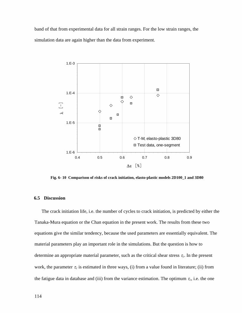
band of that from experimental data for all strain ranges. For the low strain ranges, the
simulation data are again higher than the data from experiment.
1.E-6
1.E-5
1.E-4
1.E-3
0.4 0.5 0.6 0.7 0.8 0.9
∆ε [%]
λ [-]
T-M, elasto-plastic 3D80Test data, one-segment
Fig. 6- 10 Comparison of risks of crack initiation, elasto-plastic models 2D100_1 and 3D80
6.5 Discussion
The crack initiation life, i.e. the number of cycles to crack initiation, is predicted by either the
Tanaka-Mura equation or the Chan equation in the present work. The results from these two
equations give the similar tendency, because the used parameters are essentially equivalent. The
material parameters play an important role in the simulations. But the question is how to
determine an appropriate material parameter, such as the critical shear stress τc. In the present
work, the parameter τc is estimated in three ways, (i) from a value found in literature; (ii) from
the fatigue data in database and (iii) from the variance estimation. The optimum τc, i.e. the one
114

estimated from the minimum variance estimation, is about 100MPa and is quite close to the ones
from the other two sources. The predicted relation of crack density versus the number of cycles
(the Cd-N curve) with the optimum τc in a three-dimensional, elasto-plastic model fits to the
experimental data quite well. In general, however, the τc found in literature is not a universal
constant. As a material parameter, it may depend on many factors, such as the chemical
composition and the heat treatment history of the material. Estimating τc by the fatigue limit of
the material can be a proper way when the number of cycles spent in crack propagation can be
determined and is subtracted from the failure life.
It is found that the predicted Cd-N curves coincide well with the experimental data for the
intermediate strain ranges but not for the low strain range e.g. ∆ε = 0.50%, even if the optimum
τc is used. There are a few possible reasons:
(i) The Tanaka-Mura model is based on the assumption that dislocation motion is completely
irreversible. In fact the fraction of reversible dislocation gliding can be quite high and
increases with decreasing strain range [35]. Obviously, reversible dislocation glide does not
contribute to the dislocation pile-up and in turn not to crack initiation. Venkataraman et al.
suggested a parameter f to account for the reversible dislocation in a prediction model for
crack initiation in multiple slip bands [79], where it is assumed f = 0 for complete
reversibility and f = 1 for complete irreversibility. However, no quantitative relation
between local shear amplitude and the fraction of reversible dislocation glide is available at
present. Therefore it is not possible to include this effect in the analysis presented here.
(ii) The data from experiment for ∆ε = 0.50% show quite large scatter. It is due to the nature of
fatigue behaviour, where larger scatter occurs at low strain ranges. For other strain ranges
the scatter of experimental data may be also quite large. This scatter may be caused by the
115
observation error, as mentioned in Chapter 2. There is no unambiguous procedure to
distinguish an extrusion from a crack at the given degree of resolution.
(iii) The size of the model is too small for low strain ranges. As mentioned in Chapter 4, Eq. (4-
2), the model size must be large for the simulation of low crack density. Therefore the 80-
grain model for the prediction in low strain range is not reliable.
The simulation tends to overestimates the crack initiation life for high strain ranges. A
possible reason may be that fatigue damage accumulation in each grain is not taken into account.
In the case of multiple crack initiation, the damage happens to many favourably oriented slip
bands. Certain dislocation pile-ups may have taken place along these slip bands. But in the
present simulation model only one crack is selected for initiation. In the following simulation
step, the pile-up of previous step is neglected. This leads to an overestimation of the number of
cycles to initiation.
Some influencing factors have not been dealt with by the present model, e.g. the cyclic
deformation behaviour, the accumulated damage and the surface effect. Keeping these
restrictions in mind the agreement between experimental data and simulation is quite good.
116
CHAPTER 7 CONCLUSION
The present research deals with the computer simulation for the microcrack initiation process
of a martensitic steel under low cycle fatigue. The crack initiation process is strongly influenced
by the microstructure characteristics, such as grain size and grain orientation. This fact is taken
into account in the mesoscopic models. In the elastic model the grains are modelled as single
crystals with anisotropic material behaviour. The representative volume element (RVE)
generated by a two-dimensional Voronoi-tessellation process is used to simulate the
microstructure of the polycrystalline material. A random value is assigned to each grain as the
grain orientation angle. Local stress distributions are analyzed by a general-purpose finite
element method. Successive crack initiation is simulated by defining a potential crack path
within each grain. The number of cycles to crack initiation is estimated by applying the Tanaka-
Mura equation. To investigate the effect of the three-dimensional slip system and the three-
dimensional stress state on crack initiation behaviour, a simplified 3D-RVE is used. In order to
achieve a better quantitative prediction, optimum parameter τc is determined by a parameter
study. The prediction model is based on the elasto-plastic property obtained from the cyclic
stress-strain curve. The crack density, i.e. the crack number per unit area, versus the number of
117
cycles can be determined from simulation results. From PATRAN post-processing, the stress
distribution and the crack pattern in the RVE can be obtained.
The following three main aspects are dealt with in the investigation:
- Influence of microstructural factors, such as the grain size, shape and especially the grain
orientation;
- Stress state influence, such as plane-strain and plane-stress in the two-dimensional
models and the stress in the three-dimensional models;
- Material parameters, such as anisotropic stress-strain response, elastic-plastic properties
and critical shear stress τc.
The results are composed of three parts as follows:
- The stress analyses based on uncracked RVE and on RVEs with successive initiated
cracks;
- The relations of crack density to the number of cycles to crack initiation under different
conditions;
- The crack initiation behaviour, such as the initiation sequences and crack patterns.
From the simulations, we come to the following conclusions:
- By means of the finite element analyses, the inhomogeneous stress distribution caused
by grain misorientation in the uncracked model are analyzed accurately;
- The local stress level in an individual grain varies with the grain orientation and the
magnitude of the misorientation between the neighbouring grains; high gradient stress
areas are mostly located at triple-points and/or along grain boundaries; from the
investigation of the two-dimensional model it is found that the highest von Mises stress
118
occurs in the grains which are oriented approximately ±45° to the loading axis and with
a misorientation angle to surrounding grains of about 45°.
- The simulated crack patterns, in terms of length and orientation, are quite similar to
what was observed on the specimen surfaces, i.e. in the simulation most of the initiated
cracks are from large grains and are orientated about ±45° to the loading axis;
- The stress redistribution caused by the initiated cracks is simulated; a crack may initiate
from a slip band, which lies in the enhanced stress field induced by the previously
initiated crack tip, and this crack might be either short or oriented in a low angle to the
loading axis;
- This above mentioned phenomenon appears in both elastic and elasto-plastic models for
higher strains, e.g. ∆ε = 0.76%;
- For low strain ranges, clusters of cracks are observed; for higher strain ranges the
initiated cracks are arranged in a band and tend to form a long, zigzag crack;
- In the simulation, the scatter of crack initiation life in different RVE structures is not as
significant as observed in the material;
- The crack density increases with the number of cycles and the strain ranges. This
general behaviour is reproduced with the simulation model. The simulation results
performed with the optimized parameters agree with experimental data quite well.
- By the parameter study, an optimum value of critical shear stress τc can be found.
- The structure of the three-dimensional model is more similar to the real material so that
it is suitable for the stress state analysis and grain misorientation study. The two-
dimensional model consists of more grains and finer mesh so that is suitable for the
investigation of crack initiation process.
119

The present work is a systematic research on the simulation of crack initiation. The
simulation procedure developed in the work can possibly be used for more complex problem.
120
Appendix A A.1 Transformation Matrix for Eulerian Rotation [80]
The transformation of one Cartesian coordinate system to another can be carried out by
means of three successive Z-X-Z Eulerian rotations as shown in Fig. A-1 (a)-(c). The original
coordinate system is xyz (see Fig. A-1 (a)). The first rotation is around the z-axis with angle φ
and the obtained intermediate coordinate system is zyx ′′′ . The second rotation is around x′ -
axis with angle θ and the intermediate coordinate system is zyx ′′′′′′ (see Fig. A-1 (b)). Finally
by the rotation around z′ -axis with angle ψ, the ultimate coordinate system zyx ′′′′′′′′′ is
obtained (see Fig. A-1 (c)). All rotations are performed in a counter-clockwise fashion.
121
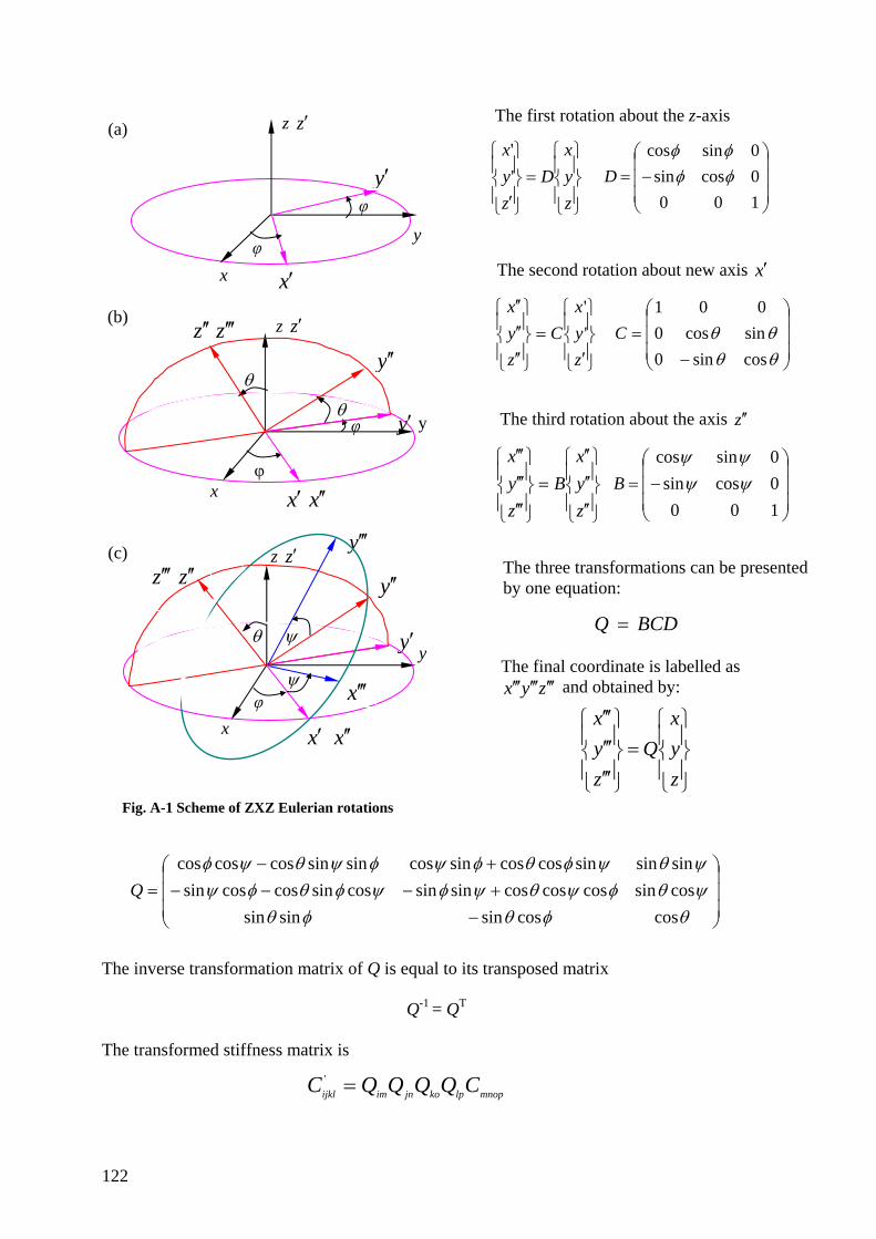
The first rotation about the z-axis
y′ y
(a)
(b)
x
z z′
yφ
φ
x′
y′
x′ x ′′
z z′
x
φ
φ
θ
θ y ′′
zz ′′′′′
⎪⎭
⎪⎬
⎫
⎪⎩
⎪⎨
⎧=
⎪⎭
⎪⎬
⎫
⎪⎩
⎪⎨
⎧
′ zyx
Dzyx''
⎟⎟⎟
⎠
⎞
⎜⎜⎜
⎝
⎛−=
1000cossin0sincos
φφφφ
D The second rotation about new axis x′
⎪⎭
⎪⎬
⎫
⎪⎩
⎪⎨
⎧
′=
⎪⎭
⎪⎬
⎫
⎪⎩
⎪⎨
⎧
′′′′′′
zyx
Czyx
''
⎟⎟⎟
⎠
⎞
⎜⎜⎜
⎝
⎛
−=
θθθθ
cossin0sincos0
001C
The third rotation about the axis z ′′
x′ x ′′
(c) z z ′
x φ
θ
z ′′′ z ′′
x ′′′
y ′′′
y
ψ
ψ
Fig. A-1 Scheme of ZXZ Eulerian rotation
⎜⎜⎜
⎝
⎛−−−
=φθ
ψφθφψφψθψφ
sinsincossincoscossinsinsincoscoscos
Q The inverse transformation matrix of Q
The transformed stiffness matrix is
imijkl QC ='
122
⎟⎟⎟
⎠
⎞
⎜⎜⎜
⎝
⎛−=
1000cossin0sincos
ψψψψ
B⎪⎭
⎪⎬
⎫
⎪⎩
⎪⎨
⎧
′′′′′′
=⎪⎭
⎪⎬
⎫
⎪⎩
⎪⎨
⎧
′′′′′′′′′
zyx
Bzyx
′
′′The three transformations can be presented by one equation:
BCDQ =
s
is
Q
y y The final coordinate is labelled as
zyx ′′′′′′′′′ and obtained by:
⎪⎭
⎪⎬
⎫
⎪⎩
⎪⎨
⎧=
⎪⎭
⎪⎬
⎫
⎪⎩
⎪⎨
⎧
′′′′′′′′′
zyx
Qzyx
⎟⎟⎟
⎠
⎞
−+−+
θφθψθφψθψφψθψφθφψ
coscossincossincoscoscossinsinsinsinsincoscossincos
equal to its transposed matrix
Q-1 = QT
mnoplpkojn CQQ
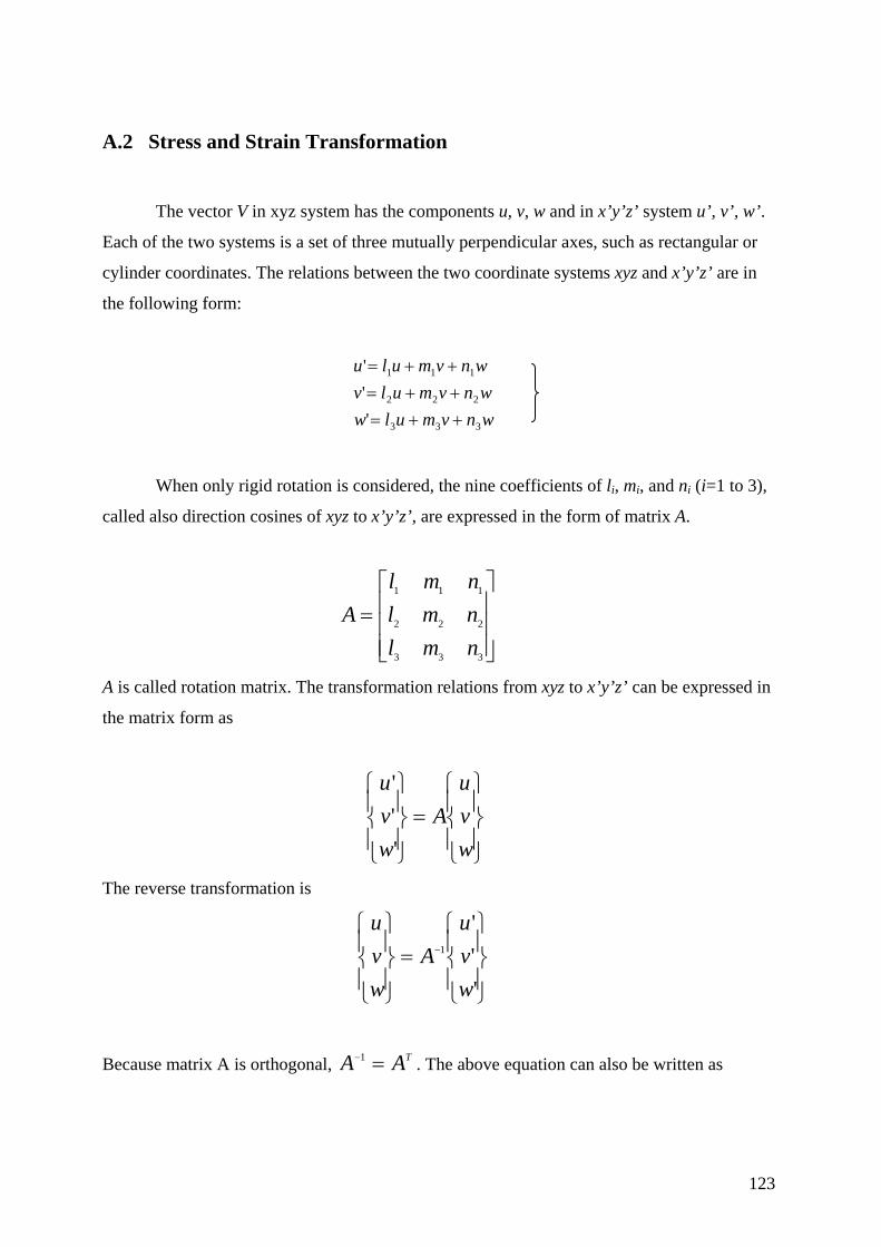
A.2 Stress and Strain Transformation
The vector V in xyz system has the components u, v, w and in x’y’z’ system u’, v’, w’.
Each of the two systems is a set of three mutually perpendicular axes, such as rectangular or
cylinder coordinates. The relations between the two coordinate systems xyz and x’y’z’ are in
the following form:
wnvmulwwnvmulv
wnvmulu
333
222
111
'''
++=++=++=
When only rigid rotation is considered, the nine coefficients of li, mi, and ni (i=1 to 3),
called also direction cosines of xyz to x’y’z’, are expressed in the form of matrix A.
⎥⎥⎥
⎦
⎤
⎢⎢⎢
⎣
⎡=
333
222
111
nmlnmlnml
A
A is called rotation matrix. The transformation relations from xyz to x’y’z’ can be expressed in
the matrix form as
⎪⎭
⎪⎬
⎫
⎪⎩
⎪⎨
⎧=
⎪⎭
⎪⎬
⎫
⎪⎩
⎪⎨
⎧
wvu
Awvu
'''
The reverse transformation is
⎪⎭
⎪⎬
⎫
⎪⎩
⎪⎨
⎧=
⎪⎭
⎪⎬
⎫
⎪⎩
⎪⎨
⎧−
'''
1
wvu
Awvu
Because matrix A is orthogonal, TAA =−1 . The above equation can also be written as
123
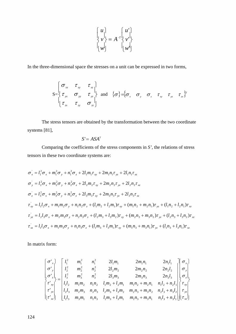
⎪⎭
⎪⎬
⎫
⎪⎩
⎪⎨
⎧=
⎪⎭
⎪⎬
⎫
⎪⎩
⎪⎨
⎧−
'''
wvu
Awvu
T
In the three-dimensional space the stresses on a unit can be expressed in two forms,
S= and ⎪⎭
⎪⎬
⎫
⎪⎩
⎪⎨
⎧
zzzyzx
yzyyyx
xzxyxx
στττστττσ
{ } { }Tzxyzxyzyx τττσσσσ =
The stress tensors are obtained by the transformation between the two coordinate
systems [81],
TASAS ='
Comparing the coefficients of the stress components in S’, the relations of stress
tensors in these two coordinate systems are:
xzyzxyzyxx nlnmmlnml τττσσσσ 11111121
21
21
' 222 +++++=
xzyzxyzyxy nlnmmlnml τττσσσσ 22222222
22
22
' 222 +++++=
xzyzxyzyxz nlnmmlnml τττσσσσ 33333323
23
23
' 222 +++++=
xzyzxyzyxxy nlnlnmnmmlmlnnmmll τττσσστ )()()( 122112211221212121' ++++++++=
xzyzxyzyxyz nlnlnmnmmlmlnnmmll τττσσστ )()()( 233223322332323232' ++++++++=
xzyzxyzyxxz nlnlnmnmmlmlnnmmll τττσσστ )()()( 133113311331313131' ++++++++=
In matrix form:
⎪⎪⎪⎪
⎭
⎪⎪⎪⎪
⎬
⎫
⎪⎪⎪⎪
⎩
⎪⎪⎪⎪
⎨
⎧
⎥⎥⎥⎥⎥⎥⎥⎥
⎦
⎤
⎢⎢⎢⎢⎢⎢⎢⎢
⎣
⎡
+++++++++
=
⎪⎪⎪⎪
⎭
⎪⎪⎪⎪
⎬
⎫
⎪⎪⎪⎪
⎩
⎪⎪⎪⎪
⎨
⎧
xz
yz
xy
z
y
x
xz
yz
xy
z
y
x
lnlnnmnmmlmlnnmmlllnlnnmnmmlmlnnmmlllnlnnmnmmlmlnnmmll
lnnmmlnmllnnmmlnmllnnmmlnml
τττσσσ
τττσσσ
133113311331311331
233223322332323232
122112211221212121
33333323
23
23
22222222
22
22
11111121
21
21
222222222
''''''
124
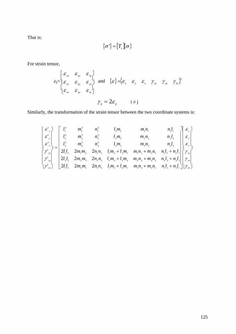
That is:
{ } [ ]{ }σσ sT='
For strain tensor,
εij= and ⎪⎭
⎪⎬
⎫
⎪⎩
⎪⎨
⎧
zzzyzx
yzyyyx
xzxyxx
εεεεεεεεε
{ } { }Tzxyzxyzyx γγγεεεε =
ijij εγ 2= i ≠ j
Similarly, the transformation of the strain tensor between the two coordinate systems is:
⎪⎪⎪
⎭
⎪⎪⎪
⎬
⎫
⎪⎪⎪
⎩
⎪⎪⎪
⎨
⎧
⎥⎥⎥⎥⎥⎥⎥
⎦
⎤
⎢⎢⎢⎢⎢⎢⎢
⎣
⎡
+++++++++
=
⎪⎪⎪
⎭
⎪⎪⎪
⎬
⎫
⎪⎪⎪
⎩
⎪⎪⎪
⎨
⎧
xz
yz
xy
z
y
x
xz
yz
xy
z
y
x
lnlnnmnmmlmlnnmmlllnlnnmnmmlmlnnmmlllnlnnmnmmlmlnnmmll
lnnmmlnmllnnmmlnmllnnmmlnml
γγγεεε
γγγεεε
133113311331311331
233223322332323232
122112211221212121
33333323
23
23
22222222
22
22
11111121
21
21
222222222
''''''
125
Appendix B
Introduction of Programs
The programs used in the simulation procedure consist of three parts:
• ‘Prelude’: a group of in-house programs, by which the files of material properties,
the grain aggregates, i.e. the Voronoi tessellation, the orientation angles and the
meshing parameters for finite element analysis models are created. The mesh
generation by PATRAN pre-processing is included in this part. The obtained files
are the input for the simulation in the next part.
• ‘Main’: a developed program package written in C. It is composed by a number of
subroutines, including the embedded ABAQUS code. It provides functions for
creating finite analysis models, computing average stresses and the number of
cycles, and introducing cracks.
• ‘Post-Show’: a manual process working with PATRAN to visualize results.
The course of the simulation is illustrated in the flowcharts in section B1. The details of
the three parts together with required input files and produced output files are given in section
B2, B3 and B4, respectively. To be concise, the star mark (*) is used as the sign representing
the alternative part of file names with the common part for the rest.
126
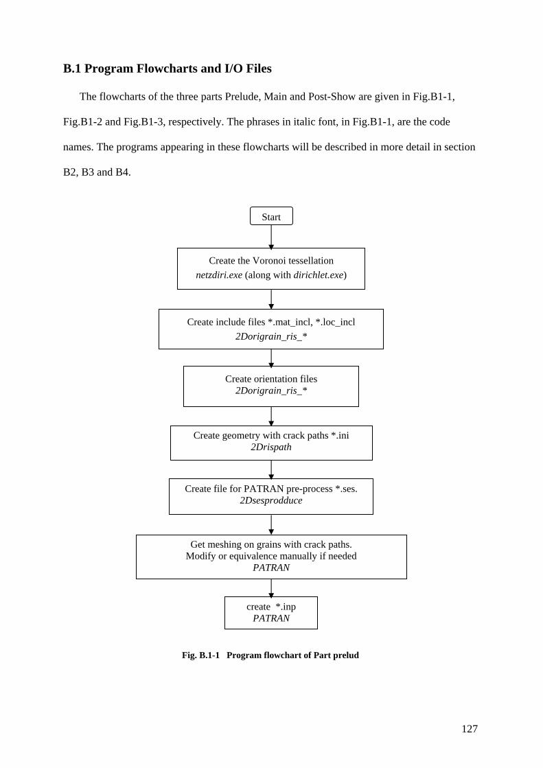
B.1 Program Flowcharts and I/O Files
The flowcharts of the three parts Prelude, Main and Post-Show are given in Fig.B1-1,
Fig.B1-2 and Fig.B1-3, respectively. The phrases in italic font, in Fig.B1-1, are the code
names. The programs appearing in these flowcharts will be described in more detail in section
B2, B3 and B4.
Start
Create the Voronoi tessellation netzdiri.exe (along with dirichlet.exe)
Create include files *.mat_incl, *.loc_incl 2Dorigrain_ris_*
Create fi
Create
Get meModify
Fig. B.1-1
Create orientation files 2Dorigrain_ris_*
le for PATRAN pre-process *.ses. 2Dsesprodduce
geometry with crack paths *.ini 2Drispath
create *.inp PATRAN
shing on grains with crack paths. or equivalence manually if needed
PATRAN
Program flowchart of Part prelud
127
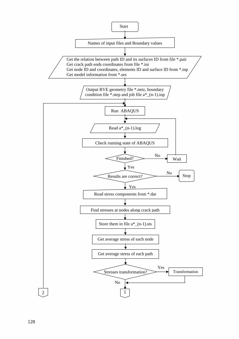
Yes No
Yes
Stop
Get average stress of each node
Store them in file a*_(n-1).sts
Stresses transformation?
No
Transformation Yes
Get average stress of each path
Find stresses at nodes along crack path
Read stress components from *.dat
Results are correct?
Wait No
Names of input files and Boundary values
Get the relation between path ID and its surfaces ID from file *.pair Get crack path ends coordinates from file *.ini Get node ID and coordinates, elements ID and surface ID from *.inp Get model information from *.ses
Check running state of ABAQUS
Read a*_(n-1).log
Output RVE geometry file *.netz, boundary condition file *.step and job file a*_(n-1).inp
Run ABAQUS
Start
Finished?
2 1
128
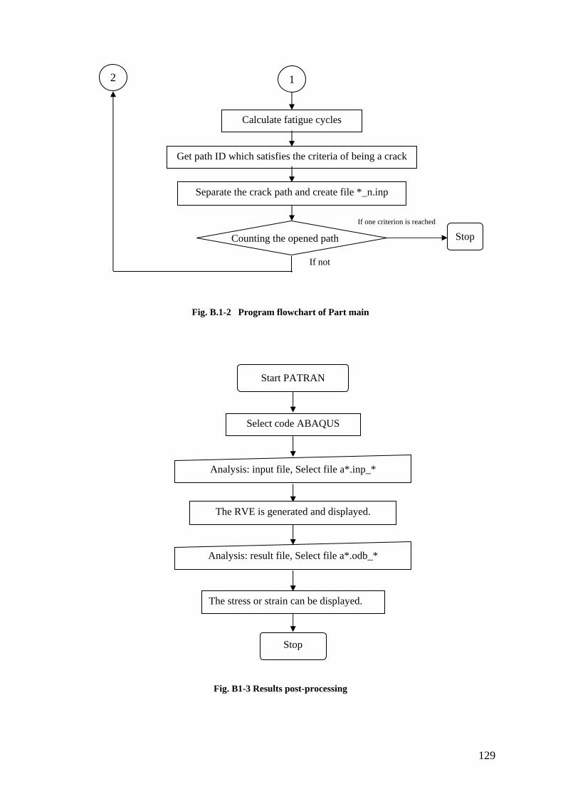
Counting the opened path
If one criterion is reached
If not
Separate the crack path and create file *_n.inp
Get path ID which satisfies the criteria of being a crack
Calculate fatigue cycles
12
Stop
Fig. B.1-2 Program flowchart of Part main Start PATRAN
Analysis: input file, Select file a*.inp_*
The RVE is generated and displayed.
The stress or strain can be displayed.
Analysis: result file, Select file a*.odb_*
Stop
Select code ABAQUS
Fig. B1-3 Results post-processing
129
B.2 Description of Programs in Part ‘Prelude’
Part Prelude includes a set of programs for completing the following tasks:
- Create the Voronoi tessellation;
- Generate grain orientation arrays;
- Transform the material tensor matrix and assign local coordinate systems to the
corresponding grains;
- Insert the crack paths into the grains;
- Write the session file.
The output files from those programs are input files for the simulation in Part ‘MAIN’.
(1) Creation of RVE Structure:
The dirichlet.exe and netz-diri.c are the two programs along with files basic.c and basic.h
to create a representative volume element with the Voronoi tessellation process. They should
be put in the same folder when running.
(2) Programs to Generate Grain Orientation and Crack Path Orientation
There are two programs: one is for the local coordinate system 2Dorigrain_ris_l.c and the
other is for the global coordinate system 2Dorigrain_ris_g.c. The functions of the above two
programs are to generate the orientation angles for the crack paths and for the virtual grains
(virtual grains refer to grains divided by crack paths).
The output files of program 2Dorigrain_ris_g are *.opa for crack paths and *.oma for
grain orientations. In file *.opa, the first value is the number of paths of the model and is equal
to the grain number. In file *.oma, the first integer is the number of virtual grains, which is
130
twice of the number of grains of the model. The angles of crack paths are the grain
orientations minus 45°. The angle assigned to each virtual grain is in the range of 0°~360°.
The output files of program 2Dorigrain_ris_l are *.ori for crack path orientation and *.orie
for grain orientation. The path orientation in *.ori is set in the range of –90°~90° and will be
used to set up the local coordinates in the next step. Since the crack paths are determined by a
given relative angle to grain orientations in local coordinates, there are only two values in file
*.orie. The first value is the number of virtual grains and the second is the angle of the crack
path to the lattice coordinate 1-axis.
(3) Programs to Insert Crack Path into Grain
Program 2Drispath.c and rissnetz.c are used to create the crack paths in the RVE. The
crack path on each grain is assumed passing through the centre of gravity of a grain and in the
orientation defined in file *.ori. By executing 2Drispath the coordinate values of the two ends
of a crack path are generated from the data in *.geo and *.ori. These data are stored in file
*.ini.
Program rissnetz.c creates a new geometry of RVE with cracks in such way that one grain
is separated by a crack path into two virtual grains according to the data in *.ini. Therefore,
the number of grains in the simulation is doubled. The geometry of RVE with crack paths is
stored in the output file *-ris.geo. Some grain boundaries are partitioned into two or three
segments by crack paths. The indices of these segments are saved in output file *-lines.out in
groups for the creation of ‘hard point’, which is a function to get coinciding notes in
PATRAN meshing.
When compiling the above programs, the following files should be put in the same folder:
basic.h, u_proto.h, basic.h, feigen.c and fpivot.c.
(4) Programs to Produce the Material Matrixes and Local Coordinate Systems
There are two programs to transform the material property matrices, 2Doriemat_g.c and
2Doriemat_l.c. When the FE output is required in the global coordinate system the program
131
2Doriemat_g.c is used. If the FE output is required in the local coordinate systems,
2Doriemat_l.c is chosen.
The program 2Doriemat_g will create a file *.mag_incl for the material matrix and a file
*.abg for the orientation vectors of the virtual grains. The file *.mag_incl is a including file
for ABAQUS, in which the stiffness matrices of the cells transformed according to the grain
orientation are stored. In the file *.abg vectors used to display grain orientation in PATRAN
images are saved. The data in each line in *.abg are the vector coordinates of each virtual
grain.
The programs 2Doriemat_l will create three files: *.mat_incl for the material matrix,
*.loc_incl for the definition of the local coordinate system and *.ab for the display of the local
coordinates in PATRAN images. The files *.mat_incl and *.loc_incl are two including files
for ABAQUS FE analyses. The file *.ab is the input file to create the local coordinate by
PATRAN pre-processing. All the parameters in the three files are given for virtual grains.
2Dorigrain_ris_lp is developed to add in plastic parameters in the file *.mat_incl for the
elasto-plastic models.
(5) Program to Create the Session File for PATRAN Pre-Processing
There are two programs for the creation of the session file. The one for the elastic model is
called 2Dsesproduce.c. The one for the elasto-plastic model is called 2Dses_p.c. These
programs are developed to create the FE model for the finite element analysis. The output file
consists of a number of PATRAN PLC functions, which are the procedures, as shown in
Table B.2-1, to create a RVE for FE analysis.
The output file *.ses is the input file for PATRAN and will be processed by PATRAN
function ‘play session’. The structure created by ‘session playing’ is a meshed RVE.
On the RVE created by PATRAN, there are some nodes which do not coincide with the
grain boundaries. These nodes have to be modified manually to get a proper RVE.
132
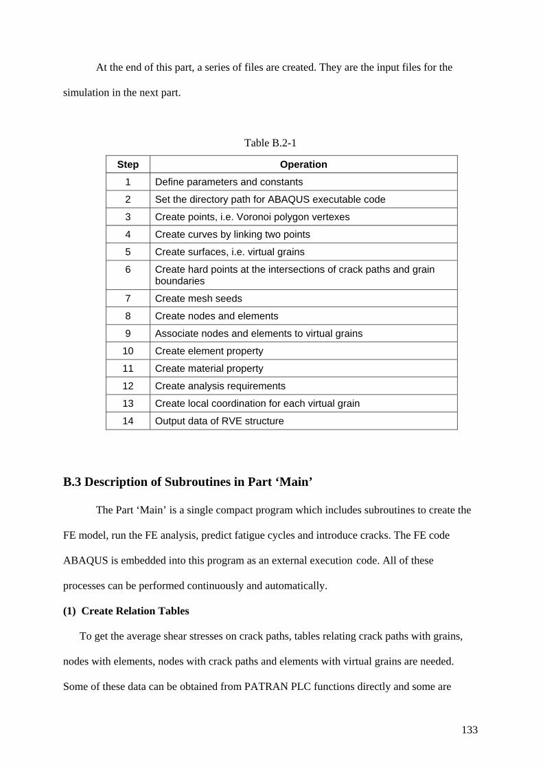
At the end of this part, a series of files are created. They are the input files for the
simulation in the next part.
Table B.2-1
Step Operation
1 Define parameters and constants
2 Set the directory path for ABAQUS executable code
3 Create points, i.e. Voronoi polygon vertexes
4 Create curves by linking two points
5 Create surfaces, i.e. virtual grains
6 Create hard points at the intersections of crack paths and grain boundaries
7 Create mesh seeds
8 Create nodes and elements
9 Associate nodes and elements to virtual grains
10 Create element property
11 Create material property
12 Create analysis requirements
13 Create local coordination for each virtual grain
14 Output data of RVE structure
B.3 Description of Subroutines in Part ‘Main’
The Part ‘Main’ is a single compact program which includes subroutines to create the
FE model, run the FE analysis, predict fatigue cycles and introduce cracks. The FE code
ABAQUS is embedded into this program as an external execution code. All of these
processes can be performed continuously and automatically.
(1) Create Relation Tables
To get the average shear stresses on crack paths, tables relating crack paths with grains,
nodes with elements, nodes with crack paths and elements with virtual grains are needed.
Some of these data can be obtained from PATRAN PLC functions directly and some are
133
derived from known parameters. These subroutines find these relations and store them in
arrays and structures.
(2) Job Files Creation
Job file is the only input file for the FE code ABAQUS. One of the main functions of
program ‘Main’ is to create a job file. A job file consists of command lines and some
including files. The including files in the job file a*.inp are: RVE geometry file *.netz,
material property file *.mat_incl, local coordinate file *.loc_incl and boundary condition file
*.step1. All of the including files have been created in Part ‘Prelude’.
(3) Running ABAQUS
The ABAQUS code is embedded and executed as a system command in the ‘Main’
program package. The program starts ABAQUS and checks the output files of ABAQUS.
ABAQUS code runs parallel with the ‘Main’ program and keeps writing output files and
information files during its process. If the ‘Main’ program finds the finish mark of ABAQUS
it starts the data processing. If an error message is obtained it reports the message and stops.
(4) FE Data Processing
The stress components at nodes are read in and only shear stresses at nodes on the crack
path are used for the average stress calculation. In result file *.dat of ABAQUS, the data of
stress components are separated into two parts, one for results of 3-node elements and the
other for 4-node elements in the two-dimensional analysis. There are two subroutines
designed for these two different output formats. The program can detect which part appears
first and run the corresponding subroutine. Calculated average stresses are stored in file *.sts.
(5) Calculation of Fatigue Cycles
The subroutine of calculation for the number of cycles is developed based on Eq. (4-8).
The constants in the equation are defined at the beginning of the program. The units in the
simulation are all in SI system and are listed here:
Stress: MPa (input) = 106 N/m2 (in program)
134

Modulus: GPa (input) = 109 N/m2 (in program)
Length: mm (input) = 10-3 m (in program)
Path length = [10-3 (grain number)1/2 ×grain size/ (X or Y size)]
(6) Criteria for Introducing a Crack
The crack path with the smallest number of cycles is selected as a crack. But if this crack
path is close to one of RVE edges, say 10% of model length, another crack with second
smallest number of cycles will be selected and so on. If the number of cycles for all crack
paths are bigger than 107 then no crack will be introduced and the program stops.
The number of cracks is an input variable at the beginning of the program. If the preset
number is reached, or if half of the crack paths have become cracks, the program stops.
(7) New Geometry Creation
With the developed subroutines the selected crack path is introduced into RVE as initiated
crack. Files with respect to the new geometry will be created, which are the input files for the
next simulation loop.
(8) Output of Fatigue Cycles
The results of fatigue cycles are stored in the file *.mylog. Some input information for the
model are stored in this file as well, including the input file names, the applied strain range,
node coordinates on crack paths, path lengths, ABAQUS running time, initiated crack path ID
and fatigue cycles.
135
Appendix C
Crack initiation sequences
It is found that the simulation results show different crack initiation sequences for
different strain ranges in the elastic model. The reason is analyzed as follows.
In all the simulation models, the crack initiation sequence, i.e. which PCP is selected
as initiated crack, depends on the number of cycles, ∆Ni, determined by the Tanaka-Mura
equation Eq. (4-8), i.e.
2)2()1(8
cresi
si
id
GWNττνπ −∆−
=∆
where ∆τres=2iτ .
The variables in Eq. (4-8) are iτ and di. Other parameters in the elastic model are
constants. Let A denote the constant part in Eq. (4-8),
)1(2
νπ −= sGWA
Eq. (4-8) can be written as:
2)( cii
i dAN
ττ −=∆ (C-1)
For a model subjected to strain ranges ε1, the induced stress on the two crack paths,
path 1 and path 2, are 1τ and 2τ respectively, where
1τ and 2τ are average shear stresses. It is
assumed that 2τ =γ
1τ , where γ is a constant. When the applied strain range is ε2 and ε2=αε1,
the magnitudes of the corresponding two stresses 1τ and
2τ are α1τ and α
2τ because the ratio
of two applied strain ranges α is maintained in elastic model. Suppose the sizes of the two
paths are d1 and d2 respectively and the size ratio of the two paths is β, i.e. d2=βd1. The above
136
mentioned variables and factors are listed in Table C-1, where τc >0, α>0, β>0,
γ>0, A>0, d>0, i.e. all the constants are positive. Additionally, the following requirements
should also be satisfied: τ >τc, γτ>τc, i.e.
1<= λττ c
Table C-1 Variables and factors of two paths under two strain ranges
Path 1 Path 2
Stress when ε1 applied1τ =τ
2τ =γ1τ =γτ
Stress when ε2 applied1τ =ατ
2τ =αγ1τ =αγτ
Path size d1=d d2=βd1= βd
Suppose the numbers of cycles to crack initiation for the two paths are ∆Ν1 and ∆Ν2
when the model is subjected to ε1 and ∆Ν’1 and ∆Ν’2 when it is subjected to ε2. Αccording to
Eq. (C-1), the above conditions can be written as:
2211
1 )()( cc dA
dAN
ττττ −=
−=∆ ,
2222
2 )()( cc dA
dAN
τγτβττ −=
−=∆
22
11
1 )()('
cc dA
dAN
τατττ −=
−=∆ ,
2222
2 )()('
cc dA
dAN
ταγτβττ −=
−=∆
If ∆ N1<∆ N2 when ε1 is applied and ∆ N’1>∆ N’2 when ε2 is applied, the crack
sequences are not the same. The following derivation is aimed to find the valid conditions
under which the above situation occurs.
1. Applied strain ε1
If ∆ N1< ∆ N2 when the applied strain is ε1, the following inequality should be valid:
22 )()( cc dA
dA
τγτβττ −<
−
Since A>0, d>0, the above inequality is written as:
22 )(1
)(1
cc τγτβττ −<
−
137
∴ 22 )()( cc τγτβττ −>−
Since τ > τc >0, β>0, γτ > τc therefore the positive square root is the solution:
)( cc τγτβττ −>− That is:
cτβτγβ )1()1( −<− (C-2) Discussion:
(1) If 01 >−β , we get 1>β and if 01 >−γβ , we get 1>γβ , i.e. 1),max( << γλβ .
The following inequality, derived from Eq. (C-2), is valid:
cτγβ
βτ11
−−
<
(2) If 01<−β and 01 >−γβ , the inequality Eq. (C-2) cannot be satisfied.
(3) If 01<−β and 01 <−γβ , we get 1<β and 1<γβ , i.e. βγ 11 << . The
following inequality is valid:
cτγβ
βτ
11
−−
>
(4) If 01 >−β and 01<−γβ , 1>β , 1<γβ , we get ),max( λβ βγ 1
<< . The
following inequality is valid:
cτγβ
βτ11
−−
>
2. Applied strain ε2
If ∆ N’1> ∆ N’2 when the model is subjected to ε2 and the following inequality should be
valid:
22 )()( cc dA
dA
ταγτβτατ −>
−
Since A>0, d>0, the above inequality becomes:
22 )(1
)(1
cc ταγτβτατ −>
−
∴ 22 )()( cc ταγτβτατ −<−
If α>1, then ατ >τc, αγτ >τc, the positive square root is the solution:
138
)( cc ταγτβτατ −<− That is:
ατγβτβ )1()1( −<− c (C-3)
Discussion:
(1) If 01 >−β and 01 >−γβ , we get: 1>β , 1>γβ , i.e. 1),max( << γλβ , and
The following inequality is valid:
ατ
γββτ c⋅
−−
>11
(2) If 01<−β and 01 >−γβ 1<β , 1>γβ , we get β
γ 1> . The following
inequality is valid:
ατ
γββτ c⋅
−−
>11
(3) If 01 <−β and 01<−γβ , we get 1<β , 1<γβ , i.e. β
γ 11 << . The following
inequality is valid:
ατ
γββ
τ c⋅−−
<11
(4) If 01 >−β and 01<−γβ , the inequality Eq. (C-3) cannot be satisfied.
3. Conclusions
Both of the inequalities for ε1, Eq. (C-2) and ε2, Eq. (C-3) should be satisfied
simultaneously. From discussions 1.(1) and 2.(1), we find, when α>1, 1>β and
1),max( << γλβ , a τ that satisfies the following inequality can be found,
cc τ
γββτ
ατ
γββ
11
11
−−
<<⋅−− (C-4)
Therefore inequality Eq. (C-4) is valid.
5. Example
139
An example is given as follows for further illustration.
Consider two crack paths, d=d1=8.812, d2=14.769, i.e. β=1.676, when α=1.529, τc
=108 and τ =τ1=254, τ2= 220, i.e. γ =0.866, λ=0.491, 7724.01=
β. These parameters
satisfy the conditions: α>1, 1>β , 1),max( << γλβ and
)262(11)171(
11
cc τ
γββτ
ατ
γββ
−−
<<⋅−−
The ratio of the number of cycles of the two paths under the two strain ranges can be
calculated by
986.0)(
)(/2
2
21 =−
−=∆∆
c
cNNττ
τγτβ
112.1)(
)('/'2
2
21 =−
−=∆∆
c
cNNτατ
ταγτβ
respectively. Therefore, for strain range ε1, the number of cycles of path 1 ∆N1 is smaller than
that of path 2 ∆N2 , i.e. ∆N1<∆N2, then path 1 is the first initiated crack. But for strain range ε2,
the number of cycles of path 2 ∆N’2 is smaller than that of path 1 ∆N’1, i.e. ∆N’2 <∆N’1, thus
path 2 is the first initiated crack.
140
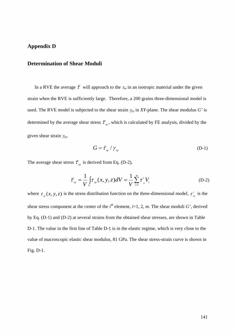
Appendix D Determination of Shear Moduli
In a RVE the average τ will approach to the τm in an isotropic material under the given
strain when the RVE is sufficiently large. Therefore, a 200 grains three-dimensional model is
used. The RVE model is subjected to the shear strain γxy in XY-plane. The shear modulus G’ is
determined by the average shear stress xyτ , which is calculated by FE analysis, divided by the
given shear strain γxy.
xyxyG γτ /= (D-1)
The average shear stress xyτ is derived from Eq. (D-2),
i
m
i
i
Vxyxy V
VdVzyx
V xy∑∫
===
1
1),,(1 τττ (D-2)
where ),,( zyxxyτ is the stress distribution function on the three-dimensional model, ixyτ is the
shear stress component at the center of the ith element, i=1, 2, m. The shear moduli G’, derived
by Eq. (D-1) and (D-2) at several strains from the obtained shear stresses, are shown in Table
D-1. The value in the first line of Table D-1 is in the elastic regime, which is very close to the
value of macroscopic elastic shear modulus, 81 GPa. The shear stress-strain curve is shown in
Fig. D-1.
141
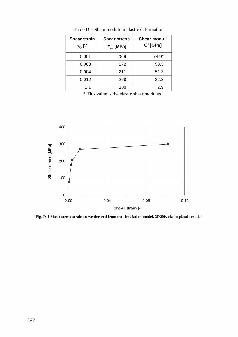
Table D-1 Shear moduli in plastic deformation
Shear strain γxy [-]
Shear stress
xyτ [MPa] Shear moduli
G’ [GPa]
0.001 78.9 78.9*
0.003 172 58.3
0.004 211 51.3
0.012 268 22.3
0.1 300 2.9 * This value is the elastic shear modulus
0
100
200
300
400
0.00 0.04 0.08 0.12
Shear strain [-]
Shea
r st
ress
[MP
a]
Fig. D-1 Shear stress-strain curve derived from the simulation model, 3D200, elasto-plastic model
142
REFERENCES
[1] Suresh, S., Fatigue of materials, 2nd version, Cambridge, 1998
[2] Brückner –Foit, A., Huang, X., and Motoyashiki, Y., Mesoscopic simulation of damage
accumulation under fatigue loading, ECF15 (The 15th European Conference of Fracture),
Stockholm, 2003
[3] Weiss, J. and Pineau, A, Continuous and sequential multiaxial low-cycle fatigue damage in
316L stainless steel, ASTM STP1191, Advances in Multiaxial Fatigue, Eds: McDowell, L. and
Ellis, R., pp. 183–203, 1993
[4] Hoshide, T. and Socie, D.F., Crack nucleation and growth modelling in biaxial fatigue, Engng.
Fract. Mech., Vol. 29, pp. 287–99, 1988
[5] Miller, K.J., The behavior of short fatigue cracks and their initiation, Fatigue & Fracture of
Engng Mater. & Struct., Vol. 10, No. 2, pp. 93–113, 1987
[6] Blochwitz, C. and Richter, J., Plastic strain amplitude dependent surface path of
microstructurally short fatigue crack in face-centred cubic metals, Mater. Science and Engng,
Vol. A367, pp. 120–29, 1999
[7] Hu, Y.M., Floer, W., Krupp, U., Christ, H. –J., Microstructurally short fatigue crack initiation
and growth in Ti –6.8Mo –4.5Fe –1.5Al, Mater. Sci. Engng, Vol. A278, pp. 170–80, 1999
[8] Long, M., Crooks, R. and. J Rack, H, High –cycle fatigue performance of solution –treated
metastable β Titanium alloys, Acta mater. Vol. 47, No. 2, pp. 661–69, 1999
[9] Polak, J., Cyclic plasticity and low cycle fatigue life of metals, Elsevier, pp. 28–32, 1991
[10] Dougherty, J.D., Srivatsan, T.S. and Padovan, J., Cyclic stress response, strain resistance and
fracture behavior of modified 1070 steel, Engng Fract. Mech., Vol. 53, No. 6, pp. 829 –847,
1996
[11] Farsetti, P. and Blarasin, A., Int. J. Fatigue, Vol. 10, pp. 153–161, 1988
[12] Carstensen, J.V., and Magnin, T., Characterization and qualification of multiple crack growth
during low cycle fatigue, Int. J. Fatigue, Vol. 23, pp. 195–200, 2003
143
[13] Wu, Z. and Sun, X., Multiple fatigue crack initiation coalescence and growth in blunt notched
specimens, Engng Fract. Mech., Vol. 59, No.3, pp. 353–59, 1998
[14] Hoshide T., Yamada, T., Fujimura, S. and Hayashi, T., Short crack growth and life prediction
in low cycle fatigue on smooth specimens, Eng Fract. Mech., Vol. 21, No.1, pp. 85–101, 1985
[15] Boyd –Lee, A.D., Fatigue crack growth resistant microstructures in polycrystalline Ni –base
superalloys for aeroengines, Int. J. of Fatigue, Vol. 21, pp. 393–405, 1999
[16] Sommer, C., Mughrabi, H., and Lochner, D., Influence of temperature and carbon content on
the cyclic deformation and fatigue behavior of α –iron, Parts I + II, Acta Materiallia, Vol. 45,
No. 5, pp. 1527–46, 1998
[17] Vasek, A. and Polak, J., Low cycle fatigue damage accumulation in ARMCO –iron, Fatigue
Fract. Engng Mater. Struct., Vol. 14, No. 2/3, pp. 193–204, 1991
[18] Han, S. –W. Kumai, S. and Sato, A., Effects of solidification structure on short fatigue crack
growth in Al–7%Si–0.4%Mg alloy castings, Materials Science and Engineering, Vol.A332, pp.
56–63, 2002
[19] Johansson, T., Kullig, E., Brückner-Foit, A. and Riesch-Oppermann, H., A fracture mechanics
model for interacting cracks in thermal fatigue, Proc. ECF 11, Vol. I, EMAS, pp. 257–62, 1986
[20] Frise PR, Bell R., Modelling fatigue crack growth and coalescence in notches, Int. J. Pressure
Vessel & Piping, Vol. 51, pp. 107–26, 1992.
[21] Tryon R.G. and Cruse T.A., A reliability –based model to predict scatter in fatigue crack
nucleation life, Fatigue & Fracture of Engng Mater. & Struct.,Vol. 21, pp. 257–67, 1998
[22] Brückner-Foit, A., Meyer, S., Möslang, A. and Diegele, E., Stochastic simulation of fatigue
damage evolution in a martensitic steel, FATIGUE 2002, Stockholm, Sweden, May, 2002
[23] Huang, X., Wu, X.R., Ding, Ch. and Hu, B.R., Small Crack propagation behavior of a forged
titanium alloy Ti –6Al –4V, FATIGUE 2002, Stockholm, Sweden, May, 2002
[24] Ewing, J.A. and Humfrey, J.C.W., The fracture of metals under repeated alternations of stress,
Philosophical transactions of the Royal Society, London, Vol. A200, pp. 241–50, 1903
[25] Mughrabi, H., The cyclic hardening and saturation behavior of copper single crystals, Mater.
Sci. Engng, Vol. 33, pp. 207–23, 1978
144
[26] Winter, A.T., A model for the fatigue of cooper at low plastic strain amplitude, Philosophical
Magazine, Vol. 29, pp. 719 –34, 1974
[27] Gong, B., Wang, Z. and Wang, Z., Cyclic deformation behavior and dislocation structures of
[001] copper single crystals –I cyclic stress –strain response and surface feature, Acta Mater.,
Vol. 45, No. 4, pp. 1365–77, 1997
[28] Pohl, K., Mayr, P., and Macherauch, E., Persistent slip bands in the interior of a fatigued low
carbon steel, Scripta Metallurgica, Vol. 14, pp. 1167–69, 1980
[29] Sasaki, S. and Ochi, Y., Some experimental studies of fatigue slip bands and persistent slip
bands during fatigue process of low carbon steel, Eng Fract. Mech. Vol. 12, pp. 531–40, 1979
[30] Man, J., Obrtlı´k, K., Blochwitz, C., Pola´k, J., Atomic force microscopy of surface relief in
individual grains of fatigued 316L austenitic stainless steel, Acta Materialia Vol. 50, pp. 3767–
80, 2002
[31] Nakai, Y., Fukuhara, S. and Ohnishi, K., Observation of fatigue damage in structural steel by
scanning atomic force microscopy, Int. J. Fatigue, Vol. 19, No. 1, pp. S223–36, 1997
[32] Ma, B. –T. and Laird, C., Overview of fatigue behaviour in copper single crystals –II.
Population size, distribution and growth kinetics of stage I cracks for tests at constant strain
amplitude, Acta Mater., Vol. 37, pp. 337–48, 1989
[33] Katagiri, K., Omura, A., Koyanagi, K., Awatani, J., Shiraishi, T., and Kaneshiro, H., Early
stage crack tip morphology in fatigued copper, Metallurgical Transactions, Vol. 8A, pp. 1769 –
73, 1977
[34] Cheng, A.S., and Laird, C., Fatigue life behavior of copper single crystals, Part I: Obser –
vations of crack nucleation, Fatigue of Engng. Mater. & Struct., Vol. 4, pp. 331–41, 1981
[35] Essmann, U., Gösele, U. and Mughrabi, H., A model of extrusions and intrusions in fatigued
metals, I. Point –defect production and the growth of extrusions, Philosophical Magazine, Vol.
A 44, pp. 405–26, 1981
[36] Lin, T.H. and Ito, Y.M., Mechanics of fatigue crack nucleation mechanism, J. Mech. Phy.
Solid, Vol. 17, pp. 511–23, 1969
[37] Tanaka, K. and Mura, T., A dislocation model for fatigue crack initiation, J. of Applied
Mechanics, Vol. 48, pp. 97–103, 1981
145
[38] Kunio, T. Shimizu, M., Yamada, K., Sakara, K. and Yamamoto, T., The early stage of fatigue
crack growth in martensitic steel, Int. J. Fract., Vol. 17, No. 2, pp. 111–19, 1981
[39] Laz, P.J., Hillberry, B.M, Fatigue life prediction from inclusion initiated cracks, Int. J. Fatigue,
Vol.30, No. 4, pp. 263–70, 1997
[40] Cheng, A.S. and Laird, C., fatigue life behavior of copper single crystals, part I and Part II. Fat.
Fract. Eng. Mater. Struct., Vol. 4, pp. 331–41, pp. 343–53, 1981
[41] Hoshide T. and Kusuura K., Life Prediction by Simulation of Crack Growth in Notched
Components with Different Microstructures under Multiaxial Fatigue, Fatigue & Fracture of
Engng Mater. & Struct., Vol. 21, pp. 201–13, 1998
[42] Zimmermann, A. and Rie, K. –T., Simulation of microcrack formation and growth during
cyclic loading considering microstructure, Fatigue 2002 –Proceedins of the 8th international
fatigue conference, Vol. 4/5, 2002
[43] Alexandre F., Deyber S. and Pineau A., Modelling the optimum grain size on the low cycle
fatigue life of a Ni based superalloy in the presence of two possible crack initiation sites,
Scripta Materialia, Vol. 50, pp. 25–30, 2004
[44] Chan, K., A microstructure –based fatigue –crack –initiation model, Metallurgical and Material
transactions A, Vol. 34A, pp. 43–58, 2003
[45] Harvey, S.E., Marsh, P.G. and Gerberich, W.W., Acta Metall. Mater., Vol. 42, pp. 3493–502,
1994
[46] Goto, M., Statistical investigations of the behavior of microcracks I carbon steel, Fatigue Fract.
Engng Mater. Struct., Vol. 14, No.8, pp. 833–45, 1991
[47] Ochi, Y., Ishii, A, Sasaki, K., An experimental and statistical investigation of surface atigue
crack initiation and growth, Fatigue Fract. Eng Mater. Struct., Vol. 8, pp. 32–39, 1985
[48] Morris, W.L., James, M.R. and Buck, O., Computer simulation of fatigue crack initiation, Eng
Fract. Mech., Vol. 13, pp. 213–21, 1980
[49] Chang, R., Morris, W.L. and Buck, O., Fatigue crack initiation at intermetallic particles in
aluminium alloy – A dislocation pile –up model, Scripta Metallurgica, Vol. 15, pp. 1941–94,
1979
146
[50] Ihara, C. and Tanaka, T., A stochastic damage accumulation model for crack initiation in high-
cycle fatigue, Fatigue Fract. Engng Mater. Struct., Vol. 23, pp. 375–80, 2000
[51] Meyer, S., Brückner –Foit, A., Möslang, A., A stochastic simulation model for micro –crack
initiation in a martensitic Steel, Computational Materials Science, Vol. 26, pp. 102–10, 2003
[52] Nemat –Nasser, S., Modelling Small Deformations of Polycrystals, edited by John Gittus and
Joseph Zarka, Elsevier Applied Science Publishers, 1986
[53] Lemaitre, J., Formulation and identi:cation of damage kinetic constitutive equations. In:
Krajcinovic, D., Lemaitre, J. (Eds.), Continuum Damage Mechanics Theory and Applications.
Springer, Wien–New York, 1987
[54] Ren, Z. –Y., Zheng, Q. –S., A Quantitative study of minimum sizes of representative volume
elements of cubic polycrystals—numerical experiments, J. Mech. & Phy. Solids, Vol. 50, pp.
881 – 93, 2002
[55] Ahmadi, A.and Zenner, H., Simulation of microcrack propagation for different load sequences,
FATIGUE 2002, Stockholm, Sweden, May, 2002
[56] Bomas, H., Hünecke, J., Laue, S. and Schöne, D., Anrisslebensdauervorhersage am Beispiel
glatter und gekerbter Proben des Werkstoffes Cm15, Mechanistenorientierte Lebensdauer –
vorhersage für zyklisch beanspruchte metallische Werkstoffe, Abschlusskolloquium des
Schwerpunktprogramms der DFG, pp. 53–68, 2004
[57] Anteboth, S., Brückner –Foit, A., Hoffmann, M.J. and Sutter, U., Simulation des elektro –
mechanischen Verhaltens von PZT mit realer Domänenstruktur, Ceramic Forum Int., DKG,
Vol. 13, pp. 179–81, 2005
[58] Kozaczek, K.J, Petrovic, S.G. and Ruud, C.O., Mcllree, A.R., Modelling of stress distribution
on the microstructural level in alloy 600, Fatigue and crack growth: Environment effects,
modeling studies and design considerations, PVP, ASME1995, Vol. 306, pp. 223–32, 1995
[59] Weyer, S., Brückner –Foit, A. and Fröhlich, A., Overall properties of ceramics subjected to
compressive loading, Int. Conf. on Engng Ceramics and Struct., Ceramic Engng and Science
Proc. Vol. 21, pp. 101–107, 2000
147
[60] Weyer S., Fr€ohlich A., Riesch-Oppermann H., Cizelj L., Kovac M., Automatic finite element
meshing of planar Voronoi tessellations, Engineering Fracture Mechanics Vol. 69, pp. 945–58,
2002
[61] Andersson, J., The influence of grain size variation on metal fatigue, Int. J. Fatigue, Vol. 27,
pp. 847–52, 2005
[62] Kumar S., Kurtz S.K., Banavar J.R. and Sharma M.G. Properties of a three –dimensional
Poisson –Voronoi tesselation: a Monte Carlo study, J. Statistics Phy., Vol. 67, pp. 523–51,
1992
[63] Bertsch, J., Mikroskopische Untersuchung der Bildung von Ermüdungsrissen an zwei ferritisch
–martensitischen Stählen im unbestrahlten und vorbestrahlten Zustand, Technik und Umwelt
Wissenschaftliche Berichte FZKA 5984, Institut für Materialforschung, Forschungs –zentrum
Karlsruhe, 1997
[64] Meyer, S., Entwicklung eines stochastischen Schädigungsmodells für einen martensitischen
Stahl unter Ermüdungsbelastung, PhD Dissertation, Universität Kassel, 2002
[65] Armas, A.F., Petersen, C., Schmitt, R., Avalos, M., Alvarez-Armas, I., Mechanical and
microstructural behavior of isothermally and thermally fatigued ferritic/martensitic steels,
Journal of Nuclear Materials, Vol. 307-311, pp. 509–13, 2002
[66] Maday, M. –F. Phenomenological aspects of fatigue cracking in as –received and hardened
F82H modifed steel exposed to lithiated water with dissolved hydrogen at 240°C, Journal of
Nuclear Materials, Vol. 283–287, pp. 68–93, 2000
[67] Li, J.C.M., Microstructure and properties of materials, Ed. J.C.M. Li, Univ. of Rochester,
World Scientific, 2000
[68] Kim, H.J., Kim, Y.H. and Morris Jr., J.M., Thermal mechanisms on grain and packet
refinement in a lath martensitic Steel, ISI J International, Vol. 38, No. 11, 1998.
[69] Guo, Z., Sato, K., Lee, T. –K. and Morris, Jr., J.W., Ultrafine grain size trough thermal
treatment of lath martensitic steels, Ultrsfine Grained Materials, TMS 2000, eds., Rajiv S.
Mishra, S.L. Semiatin etc., pp. 51–62, 2000
[70] Kelly, P.M., Jostsons, A. and Blake, RG., Acta Metall. Mater., Vol. 38, pp. 1075, 1990
148
[71] Weyer, S., Mikromechanisches Modell zur Berechnung effektiver Materialeigenschaften von
geschädigten Polykristallen, Dissertation, Univ. Karlsruhe, Germany, 2001
[72] MSC Software, PCL PATRAN 2001, Reference Manual
[73] Watanabe, O., Zbin, H.M. and Takenouchi, E., Crystal plasticity: micro –shear banding in
polycrystals using Voronoi tessellation, Int. J. Plasticity, Vol. 14, No.8, pp. 771 –789, 1998
[74] Chen, W.-F. and Saleeb, A.F., Constitutive equations for engineering materials, Vol. 1,
Elasticity and Modeling, Elsevier, 1982
[75] Kraska, M., Textursimulation bei großen inelastischen Verformungen mit der Technik des
repräsentativen Volumenelements(RVE), Pro Business, pp. 35–37, 1996
[76] Ameen, M., Computational Elasticity, Theory of elasticity and finite and boundary element
methods, Alpha Science Int. Ltd., pp. 68–77, 2005
[77] Brückner–Foit, A., and Huang, X., Numerical simulation of micro –crack initiation of
martensitic steel under fatigue loading, Int. J. Fatigue. Vol. 28, pp. 963–71, 2006
[78] Hunsche, A. and Neumann, P., Quantitative measurement of persistent slip band profiles and
crack initiation, Acta Metallurgica, Vol. 34, pp. 207–17, 1986
[79] Venkataraman, G, Chung, Y-W., Nakasone, Y. and Mura, T., Free energy formulation of
fatigue crack initiation along persistent slip bands: calculation of S-N curves and crack depths,
Acta Metall. Mater., Vol. 38, No. 1, pp. 31-40, 1990
[80] Goldstein, H., Classical Mechanics, Addison –Wesley, 1974
[81] Cook, R.D., Malkus, D. S., Plesha, M. E., Concepts and applications of finite element analysis,
3rd. edition, John Wiley & Sons, 1989
149
Erklärung
Hiermit versichere ich, dass ich die vorliegende Dissertation selbständig und ohne
unerlaubte Hilfe angefertigt und andere als die in der Dissertation angegeben
Hilfsmittel nicht benutzt habe. Alle Stellen, die wörtlich oder sinngemäß aus
veröffentlichten oder unveröffentlichten Schriften entnommen sind, habe ich als
solche kenntlich gemacht. Kein Teil dieser Arbeit ist in einem anderen Promotions-
oder Habilitationsverfahren verwendet worden.
(M.E. Xinyue Huang)


![FATIGUE CRACK INITIATION AND PROPAGATION IN … Library/101. Fatigue Crack... · 3 or predict fatigue life [15, 20]. In this paper we have conducted a detailed examination of fatigue](https://static.fdocuments.in/doc/165x107/5ab7a8aa7f8b9ad5338bd8f5/fatigue-crack-initiation-and-propagation-in-library101-fatigue-crack3-or.jpg)