Simulation of Stall Inception of a High Speed Axial

Compressor with Rotor-Stator Interaction

Jiaye Gan ∗

Hong-Sik Im †

Ge-Cheng Zha‡

Dept. of Mechanical and Aerospace Engineering, University of Miami

Coral Gables, Florida 33124, USA

August 7, 2015

Abstract

This paper solves unsteady Reynolds-averaged Navier-Stokes (URANS) equations to simulate stallinception of NASA compressor stage 35 with rotor-stator interaction. A full annulus of the rotor-statorstage is simulated with an interpolation sliding boundary condition (BC) to resolve the rotor-statorinteraction. The tip clearance is fully gridded to accurately resolve tip vortices and its effect on stallinception. The unsteady simulation indicates that the inception of rotating stall in Stage 35 is spikeinception. The stall cells grow quickly and brings the rotor to full stall within roughly 1.2 revolutions.The stall cell propagates at about 90% of rotor speed in the counter rotor rotation direction in relativethe frame.

1 Introduction

Rotating stall usually starts from tip span. The roles of tip clearance vortex, passage shock and theirinteractions on stall inception are important to understand. Tip clearance vortex breakdown is consideredas one of the causes for stall inception of some rotors[1]. For high-speed compressors, the pattern of flowbreakdown during the stall or surge is not well understood due to the effects of compressibility, difficultiesin detailed measurement, shaft speed, and geometry. Hah et al.[2] numerically studied stall inceptionin a forward-swept transonic compressor rotor. There is no tip clearance vortex breakdown during theoperation of rotor, even in the stall condition. The passage shock oscillation is considered as one of thecourses that drive the stall inception. Recently, Reuss et al.[3] tested a jet engine high pressure compressorto investigate the effect of inlet total pressure distortions on rotating stall. Their experiment shows thatthe spike type stall cell moves at approximately 60% of the compressor speed. After two to three morerevolutions, rotating stall is established. The speed of the rotating stall cell is reduced to about 45% ofthe compressor speed and its length scale is roughly 50% of the annulus.

The stall inception of NASA stage 35 is done numerically by several research groups. Mina et al.[4]carried out numerical simulation of rotating stall inception for NASA stage 35 using a single passage. Itis observed that at near stall, the tip vortex grows larger in size and its trajectory becomes perpendicularto the main axial flow. A low-momentum area near rotor tip leading edge causes the flow spillage andleads to stall inception. Davis and Yao[5] also used NASA stage 35 single blade passage to investigate stallinception. Their finding agrees with Hoying et al.[6] who shows that the circulation of tip clearance vortexplays an important role in stall inception development. Vo[7] conducted rotating stall simulation for a lowspeed rotor with relative tip Mach number of 0.2 and the transonic NASA stage 35 rotor using six blade

∗AIAA Member, Ph.D. student†AIAA Member, Ph.D., Currently a senior engineer at Honeywell‡Professor, gzha@miami.edu

1

x

y

z

Ω

Figure 1: The Cartesian system rotating with angular velocity Ω around the x-axis

passages. Their results show that leading edge tip clearance flow has spillage below blade tip and back flowat the trailing-edge at the onset of spike. Chen et al.[8, 9] conducted a full annulus simulation of NASAStage 35 at the full speed using an unsteady RANS(URANS) model. In their simulation, a simplified ”rooftop” type tip clearance mesh is used to model the tip clearance flow. Their results show that a disturbancefirst travels at the rotor speed, then changes to a spike disturbance of 84% rotor speed consisting of multiplestall cells. The disturbance eventually forms a single rotating stall cell of 43% rotor speed[8]. Most of theaforementioned Stage 35 stall inception simulation employs the ”roof top” tip griding.

The purpose of this paper is to investigate the stall inception of Stage 35 with full griding of the tipclearance to accurately simulate the stall inception. The stall inception of Stage 35 captured in this studydoes not appear to be the modal inception as obtained by Chen et al[8, 9], but a spike inception. It is notclear at this time whether the difference is from the tip clearance treatment or other numerical modelingsuch as turbulence model etc.

2 Numerical Methods

The unsteady Reynolds-averaged Navier-Stokes (URANS) equations are solved in a rotating frame[10]with the Spalart-Allmaras (SA) turbulence model[11]. A shock capturing scheme is necessary to simulatehigh-speed axial compressors since most rotor blades experience shock/boundary layer interaction. In thisstudy the Low Diffusion E-CUSP (LDE) Scheme[12] as an accurate shock capturing Riemann solver is usedwith a 3rd order WENO reconstruction for inviscid flux and a 2nd order central differencing for viscousterms[13]. An implicit 2nd order dual time stepping method[14] using unfactored Gauss-Seidel line iterationis utilized to achieve high convergence rate. The high-scalability parallel computing is implemented to savewall clock time[15].

2.1 Governing Equations

The equation of motion of fluid flow for turbomachinery in a rotating frame of reference as shownin Fig. 1 can be derived in order to take into account the Coriolis force (2Ω×V) and the centrifugalforce(Ω×Ω×r). Applying coordinate transformation to the generalized coordinate system(ξ, η, ζ), thedimensionless Reynolds averaged 3D Navier-Stokes equations coupled with the SA model can be expressedas the following conservative form:

∂Q∂t

+ ∂E∂ξ

+ ∂F∂η

+ ∂G∂ζ

= 1Re

(

∂Ev

∂ξ+ ∂Fv

∂η+ ∂Gv

∂ζ+ S

)

(1)

where Re is the Reynolds number. The equations are nondimenisonalized based on airfoil chord L∞,freestream density ρ∞, velocity U∞, and viscosity µ∞. The conservative variable vector Q, the inviscidflux vector E, the viscous flux vector Ev and the source term vector S are expressed as follows and therest can be expressed following the symmetric rule.

2

Q =1

J

ρρuρvρwρeρν

(2)

E =

ρUρuU + lxpρvU + lypρwU + lz p

(ρe + p)U − ltpρνU

(3)

Ev =

0lk τxk

lk τyk

lk τzk

lk (uiτki − qk)ρσ

(ν + ν) (l • ∇ν)

(4)

S =1

J

00

ρReRo2y + 2ρReRow

ρReRo2z − 2ρReRov

0Sv

(5)

Sv = ρcb1 (1 − ft2) Sν

+ 1Re

[

−ρ(

cw1fw −cb1

κ2 ft2

) (

νd

)2

+ ρσcb2 (∇ν)2 − 1

σ(ν + ν)∇ν • ∇ρ

]

+Re[

ρft1 (∆q)2]

(6)

where Ro is the Rossby number defined as ΩL∞

U∞. ρ is the density, p is the static pressure, and e is the total

energy per unit mass. The overbar denotes Reynolds averaged variable, and the tilde is used to denote theFavre averaged variable. ν is kinematic viscosity and ν is the working variable related to eddy viscosity inSA model. U , V and W are the contravariant velocities in ξ, η, ζ directions. For example, U is defined asfollows.

U = lt + l •V = lt + lxu + ly v + lzw (7)

lt =ξt

Jdηdζ, l =

∇ξ

Jdηdζ (8)

When the grid is stationary, lt = 0. In the current discretization, ∆ξ = ∆η = ∆ζ = 1.Let the subscripts i, j, k represent the coordinates x, y, z and use the Einstein summation convention.

By introducing the concept of eddy viscosity to close the system of equations, the shear stress τik and totalheat flux qk in Cartesian coordinates can be expressed in tensor form as

τik = (µ + µt)

[

(

∂ui

∂xk+

∂uk

∂xi

)

−2

3δik

∂uj

∂xj

]

(9)

3

qk = −

(

µ

Pr+

µt

Prt

)

∂T

∂xk

(10)

Above Eq.(9) and (10) are transformed to the generalized coordinate system in computation. The molecularviscosity µ is determined by Sutherland’s law, and µt is determined by the SA model[16].

µt = ρνfv1 (11)

wherefv1 = χ3

χ3+c3v1

, χ = νν

r = ν

ReSk2d2, S = S + ν

Rek2d2 fv2, fv2 = 1 −χ

1+χfv1

S =√

2ωijωij, ωij = 12

(

∂ui

∂xj−

∂uj

∂xi

)

The rest of auxiliary relations and the values of the coefficients given by reference[16] are used. The equationof state as a constitutive equation relating density to pressure and temperature is given as follows;

ρe =p

(γ − 1)+

1

2ρ(u2 + v2 + w2) −

1

2ρr2R2

o (12)

where r(=√

y2 + z2) is the normalized radius from the rotating axis, x. For simplicity, all the bar andtilde in above equations will be dropped in the rest of this paper.

2.2 Implicit Time Integration

The time dependent governing equation (1) is solved using dual time stepping method suggested byJameson[17]. A pseudo temporal term ∂Q

∂τis added to the governing Eq. (1). This term vanishes at the end

of each physical time step and has no influence on the accuracy of the solution. An implicit pseudo timemarching scheme using Gauss-Seidel line relaxation is employed to achieve high convergence rate insteadof using an explicit scheme[14]. The pseudo temporal term is discretized with first order Euler scheme.Let m stand for the iteration index within a physical time step, the semi-discretized governing equationcan be expressed as

[

(

1∆τ

+ 1.5∆t

)

I −

(

∂R∂Q

)n+1,m]

δQn+1,m+1

= Rn+1,m−

3Qn+1,m−4Qn+Qn−1

2∆t

(13)

where ∆τ is the pseudo time step, n is the physical time step index, and R is the net flux of the discretizedNavier-Stokes equations evaluated at a grid point.

2.3 Interpolation Rotor/Stator Sliding BC

For unsteady rotor-stator interaction simulation, the rotor mesh will rotate with the rotor blades andthe stator mesh will be stationary. Solving the Navier-Stokes equations requires transferring the fluxesbetween these two meshes. In [18], a conservative sliding BC is developed by making the meshes on bothside of the sliding boundary one-to-one connected. Even though the conservative BC is mathematicallymore rigorous, it is not convenient to make a multi-block mesh one-to-one connected. For engineeringapplications, independent mesh for rotor and stator is desirable for efficient setup of a simulation. Thispaper thus adopts an interpolation sliding BC with high accuracy to remove the requirement that the rotorand stator mesh needs to be one-to-one connected.

The working mechanism of present interpolation rotor/stator sliding BC is sketched in Fig. 2, whereS1, S2, S3, S4 and R1, R2, R3 are the arbitrary computational mesh cells of the stator and rotor inthe circumferential direction on the two sides of the sliding interface. The current interpolation slidingboundary condition is based on the same radial distribution of the mesh on both side of the slidingboundary.

4

Rot

orSta

tor

X

Y

Z

S4

R1

S2

S3

R1

R2

S1

S1

R3

θS1

Lower boundary

Upper boundary

Upper boundary

Lower boundary

Overlap region

ϕ

Figure 2: Working mechanism of interpolation rotor/stator sliding BC

To interpolate the conservative variable vector Q, the circumferential mesh angle is first obtained ateach mesh cell center, e.g. the angle of a stator cell s1, θs1 can be defined as tan−1(z/y)s1. Then, twoadjacent mesh angles in the opposite interface corresponding to current mesh cell are found for linearinterpolation, e.g. Q at R3 is interpolated in terms of (θR3 − θS2) and (θS3 − θS2) as given in Eq. (14).Note that a rotation rule based on the geometric periodicity is used to interpolate Q in the non-overlapregion, e.g. QS1 is rotated by the periodic sector angle (ϕ) to interpolate QR1 vice versa for QR1.

QR3 =θR3 − θs2

θs3 − θs2(Qs3 − Qs2) + Qs2 (14)

Since the frame of reference taken in this study is a fixed frame for the stationary blades and a movingrelative frame for the rotor, the following exchange relations between the fixed and moving relative frameare used.

ρρuρvr

ρ(vθ + rRo)ρ(e + cθrRo)

F ixed

ρρuρvr

ρvθ

ρe

Moving

(15)

2.4 Other Boundary Conditions

At the inlet, the radial distributions of total pressure, total temperature, swirl angle and pitch angle arespecified and the velocity is extrapolated from the computational domain in order to determine the rest ofthe variables. On the blade surface a non-slip boundary condition is applied, while an efficient wall functionBC[10] is used on the hub/casing surface where y+ is greater than 11 to avoid an excessive fine mesh in theendwall boundary layer. At the stator outlet, the static pressure is specified in the spanwise direction. Thevelocity components are extrapolated from the computational domain and an isentropic relation is used todetermine density. The hub/casing wall static pressure for the inviscid momentum equation is determinedby solving the radial equilibrium equation, whereas the static pressure gradient across the wall boundaryis set to zero for the blade wall surface. An adiabatic condition is used to impose zero heat flux throughthe wall.

5

3 Results and discussion

The transonic axial compressor, NASA stage 35 that consists of 36 rotor blades and 46 stator blades[19],is simulated to investigate the stall inception mechanism using the interpolation rotor/stator sliding BC.The total pressure ratio of NASA stage 35 at design speed of 17189 rpm is 1.82. Full annulus of stage35 with geometry periodic sector simulated and the mesh is shown in Fig.3. An O-mesh topology aroundblades and H-mesh for stage inlet/outlet duct region are used. The rotor tip clearance is modeled usinga fully grided O-mesh. In the tip gap, 11 grid points are placed radially. Total mesh points of the fullannulus are about 16 million with 482 blocks. The physical time step size is determined to allow about 40unsteady steps per rotor blade passing.

Figure 3: Full annulus mesh of NASA stage 35

Fig.4 shows the predicted speedline for NASA Stage 35 using steady state single blade passage withmixing plane boundary condition on the rotor and stator interface. A refined mesh of total 550,750 gridpoints and a coarse mesh (main mesh) of 449,790 grid points per blade passage are used for the meshrefinement study using the mixing plane[18]. The speedline predicted by the two meshes shows goodagreement. Therefore, the coarse mesh is used to construct the full annulus mesh in Fig.3. The simulationis conducted at 4004 test condition[19] since the measured radial profiles for CFD comparison are available.The mass flows at choke condition predicted by both unsteady rotor/stator interaction and steady mixingplane are about 20.82 kg/s, which is about 0.62% lower than the measured choke flow of 20.95 kg/s[19].

The circumferential mass averaged total pressure ratio, total temperature ratio, adiabatic efficiencyand absolute flow angle at stage outlet are compared with the measurement at 4004 point[19] in Fig.5.Overall good agreement with the experiment is achieved by both approaches; the mixing plane and theinterpolation rotor/stator sliding BC.

Fig.6 shows instantaneous entropy at mid span of the compressor. The wake propagates well throughthe rotor/stator interface smoothly. Fig.7 compares the instantaneous normalized mass flux ρU (top)and static pressure P (bottom) right upstream and downstream of the interface, which indicates excellentflux conservation through the rotor/stator interface. Fig.6 and Fig.7 use the half annulus to validate theinterpolating sliding BC. The simulation of stall inception in the following section employs full annulus.

3.1 Stall Pressure Rise Characteristics

The predicted unsteady stage speedline is illustrated in Fig.8, which starts from the near stall point P2.It can be seen that pressure drop is after the near stall point is nearly linear. Fig.9 shows the variationsof mass flow rate during rotating stall. Although the pressure rise start to drop at P2 as shown in Fig.8,

6

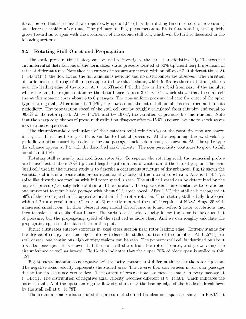
it can be see that the mass flow drops slowly up to 1.0T (T is the rotating time in one rotor revolution)and decrease rapidly after that. The primary stalling phenomenon at P4 is that rotating stall quicklygrows toward inner span with the occurrence of the second stall cell, which will be further discussed in thefollowing sections.

3.2 Rotating Stall Onset and Propagation

The static pressure time history can be used to investigate the stall characteristics. Fig.10 shows thecircumferential distributions of the normalized static pressure located at 50% tip chord length upstream ofrotor at different time. Note that the curves of pressure are moved with an offset of 2 at different time. Att=14.0T(P3), the flow aound the full annulus is periodic and no disturbances are observed. The variationof static pressure through full annuls appear to have sharp shape, which indicates there exit strong shocksnear the leading edge of the rotor. At t=14.5T(near P4), the flow is disturbed from part of the annulus,where the annulus region containing the disturbance is from 310 ∼ 10, which shows that the stall cellsize at this moment cover about 5 to 6 passages. The non-uniform pressure indicate the onset of the spiketype rotating stall. After about 1.1T(P9), the flow around the entire full annulus is disturbed and lose itsperiodicity. The propagation speed of the stall cell can be roughly calculated from this plot and equal to90.0% of the rotor speed. At t= 15.75T and t= 16.0T, the variation of pressure become random. Notethat the sharp edge shapes of pressure distribution disapper after t=15.5T and are lost due to shock wavesmove to more upstream.

The circumferential distributions of the upstream axial velocity(Ux) at the rotor tip span are shownin Fig.11. The time history of Ux is similar to that of pressure. At the beginning, the axial velocityperiodic variation caused by blade passing and passage shock is dominant, as shown at P3. The spike typedisturbance appear at P4 with the disturbed axial velocity. The non-periodicity continues to grow to fullannulus until P9.

Rotating stall is usually initiated from rotor tip. To capture the rotating stall, the numerical probesare hence located about 50% tip chord length upstream and downstream at the rotor tip span. The term’stall cell’ used in the current study is to describe a continuous structure of disturbances. Fig.12 shows thevariations of instantaneous static pressure and axial velocity at the rotor tip upstream. At about 14.5T, aspike like disturbance travling with full rotor speed is seen. The stall cell speed can be determined by theangle of pressure/velocity field rotation and the duration. The spike disburbance continues to rotate andand transport to more blade passage with about 90% rotor speed. After 1.5T, the stall cells propagate at50% of the rotor speed in the opposite direction of the rotor rotation. The rotating stall is fully developedwithin 1.2 rotor revolutions. Chen et al.[8] recently reported the stall inception of NASA Stage 35 withnumerical simulation. In their observations, modal disturbance is found before 2 rotor revolutions andthen transform into spike disturbance. The variations of axial velocity follow the same behavior as thatof pressure, but the propagating speed of the stall cell is more clear. And we can roughly calculate thepropagating speed of the stall cell from this plot.

Fig.13 illustrates entropy contours in axial cross section near rotor leading edge. Entropy stands forthe degree of energy loss, and high entropy reflects the stalled portion of the annulus. At 14.57T(nearstall onset), one continuous high entropy regions can be seen. The primary stall cell is identified by about5 stalled passages. It is shown that the stall cell starts from the rotor tip area, and grows along thecircumference as well as inward. Fig.13 also indicates that the upper 70% of blade span is stalled within1.2T.

Fig.14 shows instantaneous negative axial velocity contour at 4 different time near the rotor tip span.The negative axial velocity represents the stalled area. The reverse flow can be seen in all rotor passagesdue to the tip clearance vortex flow. The pattern of reverse flow is almost the same in every passage att=14.44T. The distribution of negative axial velocity becomes different at t=14.56T, which indicates theonset of stall. And the upstream regular flow structure near the leading edge of the blades is breakdownby the stall cell at t=14.78T.

The instantaneous variations of static pressure at the mid tip clearance span are shown in Fig.15. It

7

is seen from this figure that the flow near the leading edge of some blade passages is disturbed due to theinteraction of shock wave and tip clearance vortex at t=14.44T, which indicates the stall inception of thecompressor. As the rotor rotating, the stall cell propagates in the opposite direction of rotor revolutionand grows rapidly. The flow blockage region becomes bigger and bigger and the unsymmetrical pressuredistribution around the circumference can be detected. At t=15.0T, the non-uniform flow near the tip spancovers most of the rotor passages. Furthermore, it is evident that the rotating stall diffuses very rapidlydownstream of rotor and interacts with stator, which creates a significant amount of unsteadiness.

Fig.16 shows the relative Mach number contours across the 6 rotor blade passages where the stallinception occurs. At t=14.11T, the detached shock waves are uniform and close to the leading edge ofrotor blade. The shock wave and tip vortex interaction phenomena at suction side can be observed. Theshock wave fronts are pushed further upstream by the flow blockage and become non-uniform at t=14.56T.After t=15.0T, it can be seen that the shock wave fronts are almost disappear in upstream region of rotor.And low momentum flow covers most of leading edge near the tip span. It is note that the stall cellat the original location grows slowly in the direction of casing to hub as most of shock wave dominatedflow structures are uniform since the 75% span, which indicates the propagating speed of stall cell incircuferencial direction is much faster than the speed in inward direction. This can also be seen in Fig.13.

The vortex cores and surrounded streamlines identified in the rotor passage are illustrated in Fig.17. Att=14.11T away from the stall inception, the trajectory of the tip vortex is oblique and may interact withpressure side of adjacent blades. At t=14.56T near stall inception, the trajectory of the vortex core is alignperpendicularly to the axial direction which indicates the spikes like stall inception as discussed Hoying[6].However, the tip vortex breakdown phenomena are not clearly seen during the stall onset. The tip vortexbreakdown occurrence is used as a criteria for the cause of stall inception by many people[20, 21, 22, 23, 1].In present study, there is no breakdown to the tip clearance vortex occurred during the onset of the stall.The breakdown of the tip clearance vortex happen after t=14.78T.

4 Conclusions

The URANS was conducted to investigate rotating stall inception mechanism in a full annulus tran-sonic rotor NASA Stage 35 with sliding interpolation BC. The predicted stage performance have a goodagreement with the experiment. The details of the flow breakdown that lead to fully developed rotatingstall are well captured by the present numerical methods.

The simulation shows that the rotor stall onset is spike like disturbance with inlet total pressureperturbation. The stall disturbance at the rotor tip span propagation starts at the speed of at 100% of therotor speed in the opposite direction of rotor rotation. The size of the onset stall cell cover about 5 to 6rotor blade passage. The stall inception occurs at roughly 14.5T. The stall cell grows to the whole annulusroughly within 1.2 rotor revolutions after the stall inception. The propagation speed of stall cell is about90% of rotor rotating speed.

The tip clearance vortex breakdown was not observed in present study during the the onset of stall.The interaction between shock wave and tip leakage vortex appears to be the cause of stall. The trajectoryof tip clearance vortex is perpendicular to the leading edge when the rotor begins to stall.

Acknowledgment

The grant support from AFRL and the industrial partners of GUIde Consortium, 10-AFRL-1024 and09-GUIDE-1010, are acknowledged.

8

Mass flow rate, kg/s

Sta

geto

talp

ress

ure

ratio

18 19 20 211.6

1.7

1.8

1.9

2

ExperimentMP - finer meshMP - main meshSliding - half annulus at 4004

4004

Figure 4: Predicted speedline of NASA stage 35

Stage total pressure ratio

%S

pan

1.2 1.4 1.6 1.8 20

20

40

60

80

100

ExperimentMP - main meshMP - finer meshSliding - main mesh

Stage total temperature ratio

%S

pan

1.15 1.2 1.25 1.30

20

40

60

80

100

ExperimentMP - main meshMP - finer meshSliding - main mesh

Stage adiabatic efficiency

%S

pan

0.2 0.4 0.6 0.8 10

20

40

60

80

100

ExperimentMP - main meshMP - finer meshSliding - main mesh

Stage outlet absolute flow anget, deg

%S

pan

0 5 10 15 20 25 300

20

40

60

80

100

ExperimentMP - main meshMP - finer meshSliding - main mesh

Figure 5: Predicted pitch averaged radial profiles at 4004 including stage total pressure ratio, totaltemperature ratio, adiabatic efficiency and outlet absolute flow angle

9

Figure 6: Instantaneous entropy contour at mid span of NASA stage 35

Mesh circumferential angle, deg

Nor

mal

ized

mas

sflu

x(

U)

-90 -45 0 45 90 135 180

0.6

0.9

1.2

1.5

1.8

Rotor side interfaceStator side interface

ρ

0 15 30 45 60 75 901

1.2

1.4

1.6

1.8

Mesh circumferential angle, deg

Nor

mal

ized

stat

icpr

essu

re(P

)

-90 -45 0 45 90 135 180

3.4

3.6

3.8

4

4.2Rotor side interfaceStator side interface

Figure 7: Instantaneous normalized mass flux ρU (top) and static pressure P (bottom) at mid span ofthe rotor/stator interface

10

Mass flow rate, kg/s

Tot

alpr

essu

rera

tio14 15 16 17 18 19 20 21

1.6

1.7

1.8

1.9 P1P2

P3P4

P5P6

P8

P7

P9

Figure 8: Predicted unsteady speedline with full annulus simulation

Rotor revolution

Mas

sflo

wra

te,k

g/s

13 14 15 16 17 180

5

10

15

20

InletOutlet

P1

P2

P3

P4

P8

P5

P6P7

P9

Figure 9: Mass variation during stall

11

Time

Circ

umfe

rent

iala

ngle

,deg

0

60

120

180

240

300

360

t=14.0 T t=16.0 T

t=14.25T

t=14.50T

t=14.75T

t=15.0T

t=15.25T t=15.75T

t=15.50T

Figure 10: Time traces of circumferential pressure at tip span

Time

Circ

umfe

rent

iala

ngle

,deg

0

60

120

180

240

300

360

t=14.0 T t=16.0 T

t=14.25T

t=14.50T

t=14.75T

t=15.0T

t=15.25T t=15.75T

t=15.50T

Figure 11: Time traces of circumferential axial velocity at tip span

Rotor revolution13 14 15 16 17 18 19 20

Blade 36

Blade 1

Rotating

direction

Rotor revolution13 14 15 16 17 18 19 20

Blade 36

Blade 1

Rotating

direction

Figure 12: Variations of pressure and axial velocity at tip span

12

Figure 13: Entropy change of axial cross section near rotor leading edge

13

Figure 14: Contour of negative axial velocity at the rotor tip span

14

Figure 15: Static pressure at the tip clearance

15

Figure 16: Mach contours across the starting stall cell

16

Figure 17: Tip clearance vortex trajectory at different instances

17

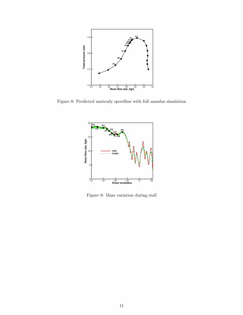
References

[1] K. Yamada, M. Furukawa, and K. Funazaki, “Numerical Analysis of Tip Leakage Flow Field in aTransonic Axial Compressor Rotor.” IGTC2003 Tokyo TS-030, Proceedings of the International GasTurbine Congress 2003, 2003.

[2] C. Hah, D.C. Rabe, and A.R. Wadia, “Role of Tip-Leakage Vortices and Passage Shock in StallInception in a Swept Transonic Compressor Rotor.” GT2004-53867, Proceedings of ASME TurboExpo 2004, 2004.

[3] N. Reuss, and C. Mundt, “Experimental Investigations of Pressure Distortions on the High-PressureCompressor Operating Behavior,” Journal of Propulsion and Power, vol. 25, pp. 653–667, doi:10.2514/1.37412, 2009.

[4] M. Zake, L. Sankar, and S. Menon, “Hybrid Reynolds-Averaged Navier-Stokes/Kinetic-Eddy Simula-tion of Stall Inception in Axial Compressors,” Journal of Propulsion and Power, vol. 26, pp. 1276–1282,doi: 10.2514/1.50195, 2010.

[5] R. Davis, and J. Yao, “Computational Approach for Predicting Stall Inception in Multistage AxialCompressor,” Journal of Propulsion and Power, vol. 23, pp. 257–265, doi: 10.2514/1.50195, 2007, doi:10.2514/1.18442.

[6] D.A. Hoying, C.S. Tan, H.D. Vo, and E.M. Greitzer, “Role of Blade Passage Flow Structuresin Axial Compressor Rotating Stall Inception,” AMSE J. of Turbomach., vol. 121, pp. 735–742,doi:10.1115/1.2836727, 1999.

[7] H.D. Vo, C.S. Tan, and E.M. Greitzer, “Criteria for Spike Initiated Rotating Stall,” AMSE J. of

Turbomach., vol. 130, pp. 1–8, doi:10.1115/1.2750674, 2008.

[8] J. Chen, B. Johnson, M. Hathaway, and R. Webster, “Flow Characteristics of Tip Injection on Com-pressor Rotating Spike via Time-Accurate Simulation,” Journal of Propulsion and Power, vol. 25,pp. 678–687, doi: 10.2514/1.41428, 2009.

[9] J. Chen, M. Hathaway, and G. Herrick, “Prestall Behavior of a Transonic Axial CompressorStage via Time-Accurate Numerical Simulation,” AMSE J. of Turbomach., vol. 130, pp. 1–12,doi:10.1115/1.2812968, 2008.

[10] H.S. Im, X.Y. Chen, and G.C. Zha, “Detached Eddy Simulation of Stall Inception for a FullAnnulus Transonic Rotor,” Journal of Propulsion and Power, vol. 28 (No. 4), pp. 782–798, doi:10.2514/1.58970, 2012.

[11] P.R. Spalart, W.H. Jou, M. Strelets, and S.R. Allmaras, “Comments on the Feasibility of LES forWings, and on a Hybrid RANS/LES Approach.” Advances in DNS/LES, 1st AFOSR Int. Conf. onDNS/LES, Greyden Press, Columbus, H., Aug. 4-8, 1997.

[12] G.C. Zha, Y.Q. Shen, and B.Y. Wang, “An Improved Low Diffusion E-CUSP Upwind Scheme ,”Journal of Computer and Fluids, vol. 48, pp. 214–220, 2011, doi:10.1016/j.compfluid.2011.03.012.

[13] Y.Q. Shen, G.C. Zha, and B.Y. Wang, “Improvement of Stability and Accuracy of Implicit WENOScheme,” AIAA Journal, vol. 47, pp. 331–334, DOI:10.2514/1.37697, 2009.

[14] Y.Q. Shen, B.Y. Wang, and G.C. Zha, “Implicit WENO Scheme and High Order Viscous Formulasfor Compressible Flows .” AIAA Paper 2007-4431, 2007.

[15] B. Wang, Z. Hu, and G. Zha, “A General Sub-Domain Boundary Mapping Procedure For Struc-tured Grid CFD Parallel Computation,” AIAA Journal of Aerospace Computing, Information, and

Communication, vol. 5, pp. 425–447, 2008.

18

[16] P.R. Spalart, and S.R. Allmaras, “A One-equation Turbulence Model for Aerodynamic Flows.” AIAA-92-0439, 1992.

[17] A. Jameson, “Time Dependent Calculations Using Multigrid with Applications to Unsteady FlowsPast Airfoils and Wings.” AIAA Paper 91-1596, 1991.

[18] H.S. Im, X.Y. Chen, and G.C. Zha, “Simulation of 3D Multistage Axial Compressor Using a FullyConservative Sliding Boundary Condition.” ASME IMECE2011-62049, International Mechanical En-gineering Congress & Exposition, Denver, November 2011, 2011.

[19] L. Reid, and R.D. Moore, “Design and Overall Performance of Four Highly-Loaded, High Speed InletStages for an Advanced, High Pressure Ratio Core Compressor.” NASA TP.1337, 1978.

[20] Adamczyk, J. J., Celestina, M. L., and Greitzer, E. M., “The Role of Tip Clearance in High-SpeedFan Stall,” Journal of Turbomachinery, vol. 115, pp. 22–38, 1993.

[21] W. W. Copenhaver, E. R. Mayhew, E. R., C. Hah, and A. R. Wadia, “The Effects of Tip Clearanceon a Swept Transonic Compressor Rotor,” Journal of Turbomachinery, vol. 118, pp. 230–239, 1996.

[22] D. E. Van Zante, A. J. Strazisar, J. R. Wood, M. D. Hathaway, T. H. Okiishi, “Recommendationsfor Achieving Accurate Numerical Simulation of the Tip Clearance Flows in a Transonic CompressorRotor,” Journal of Turbomachinery, vol. 122, pp. 733–742, 2000.

[23] D. C. Rabe, C. Hah, “Application of Casing Circumferential Grooves for Improved Stall Margin in aTransonic Axial Compressor.” ASME Paper GT-2002-30641, 2002.

19