Modification of axial-flow compressor stall margin by ...

Retrospective Theses and Dissertations Iowa State University Capstones, Theses andDissertations

1991

Modification of axial-flow compressor stall marginby variation of stationary blade setting anglesJohn Paul RukavinaIowa State University

Follow this and additional works at: https://lib.dr.iastate.edu/rtd

Part of the Mechanical Engineering Commons

This Dissertation is brought to you for free and open access by the Iowa State University Capstones, Theses and Dissertations at Iowa State UniversityDigital Repository. It has been accepted for inclusion in Retrospective Theses and Dissertations by an authorized administrator of Iowa State UniversityDigital Repository. For more information, please contact [email protected].

Recommended CitationRukavina, John Paul, "Modification of axial-flow compressor stall margin by variation of stationary blade setting angles " (1991).Retrospective Theses and Dissertations. 9575.https://lib.dr.iastate.edu/rtd/9575

http://lib.dr.iastate.edu/?utm_source=lib.dr.iastate.edu%2Frtd%2F9575&utm_medium=PDF&utm_campaign=PDFCoverPages

http://lib.dr.iastate.edu/?utm_source=lib.dr.iastate.edu%2Frtd%2F9575&utm_medium=PDF&utm_campaign=PDFCoverPages

https://lib.dr.iastate.edu/rtd?utm_source=lib.dr.iastate.edu%2Frtd%2F9575&utm_medium=PDF&utm_campaign=PDFCoverPages

https://lib.dr.iastate.edu/theses?utm_source=lib.dr.iastate.edu%2Frtd%2F9575&utm_medium=PDF&utm_campaign=PDFCoverPages

https://lib.dr.iastate.edu/theses?utm_source=lib.dr.iastate.edu%2Frtd%2F9575&utm_medium=PDF&utm_campaign=PDFCoverPages

https://lib.dr.iastate.edu/rtd?utm_source=lib.dr.iastate.edu%2Frtd%2F9575&utm_medium=PDF&utm_campaign=PDFCoverPages

http://network.bepress.com/hgg/discipline/293?utm_source=lib.dr.iastate.edu%2Frtd%2F9575&utm_medium=PDF&utm_campaign=PDFCoverPages

https://lib.dr.iastate.edu/rtd/9575?utm_source=lib.dr.iastate.edu%2Frtd%2F9575&utm_medium=PDF&utm_campaign=PDFCoverPages

mailto:[email protected]

INFORMATION TO USERS

This manuscript has been reproduced from the microfilm master. UMI fihns the text directly from the original or copy submitted. Thus, some thesis and dissertation copies are in typewriter face, while others may

be from aiiy type of computer printer.

The quality of this reproduction is dependent upon the quality of the

copy submitted. Broken or indistinct print, colored or poor quality illustrations and photographs, print bleedthrough, substandard margins, and improper alignment can adversely affect reproduction.

In the unlikely event that the author did not send UMI a complete manuscript and there are missing pages, these will be noted. Also, if unauthorized copyright material bad to be removed, a note will indicate the deletion.

Oversize materials (e.g., maps, drawings, charts) are reproduced by sectioning the original, beginning at the upper left-hand corner and continuing from left to right in equal sections with small overlaps. Each original is also photographed in one exposure and is included in

reduced form at the back of the book.

Photographs included in the original manuscript have been reproduced xerographically in this copy. Higher quality 6" x 9" black and white photographic prints are available for any photographs or illustrations appearing in this copy for an additional charge. Contact UMI directly to order.

University Microfilms International A Bell & Howell Information Company

300 North! Zeeb Road. Ann Arbor, Ml 48106-1346 USA 313/761-4700 800/521-0600

Order Number 0126243

Modification of axial-flow compressor stall margin by variation of stationary blade setting angles

Rukavina, John Paul, Ph.D.

Iowa State University, 1991

U M I 300N.ZcebRd. Ann Aibor, MI 48106

NOTE TO USERS

THE ORIGINAL DOCUMENT RECEIVED BY U.M.I. CONTAINED PAGES

WITH POOR PRINT. PAGES WERE FILMED AS RECEIVED.

THIS REPRODUCTION IS THE BEST AVAILABLE COPY.

Modification of axiai-flow compressor stall margin

by variation of stationary blade setting angles

John Paul Rukavina

A Dissertation Submitted to the

Graduate Faculty in Partial Fulfillment of the

Requirements for the Degree of

DOCTOR OF PHILOSOPHY

Major: Mechanical Engineering

by

I ' " 'nk

For the Major Department

For the Graduate College

Iowa State University Ames, Iowa

1991

Signature was redacted for privacy.



ii

TABLE OF CONTENTS

NOMENCLATURE xiv

ABSTRACT xviii

1. INTRODUCTION . . . 1

1.1 Stall 4

1.2 Surge 7

1.3 Avoiding Stall 8

2. RELATED ISOLATED AIRFOIL DYNAMIC STALL RESEARCH 12

3. PROOF OF CONCEPT IN LOW-SPEED COMPRESSORS . . 24

3.1 Stationary Blade Setting Angle Variations 25

3.2 Two-Stage Axial-Flow Fan 29

3.2.1 Two-stage fan performance tests 31

3.2.2 Axial-flow fan results . 33

3.3 Three-Stage Axial-Flow Compressor 39

3.3.1 Three-stage compressor performance tests 43

3.3.2 Three-stage compressor results 45

3.4 Detailed Flow Measurements for Three-Stage Compressor 57

3.4.1 Velocity diagram calculations using detailed measurements . . 67

iii

3.5 Low-Speed Compressor Conclusions 74

. 4. PRATT & WHITNEY COMPRESSOR 78

4.1 Pratt & Whitney Axial-Flow Compressor 78

4.1.1 D.C. drive motor and gearbox 83

4.1.2 Throttle 83

4.1.3 Surge detection and relief system 84

4.2 Pratt & Whitney Compressor Data Acquisition System 88

4.2.1 Pressure system 88

4.2.2 Temperature system 106

4.3 Pratt k Whitney Three-Stage Compressor Performance Tests .... 108

4.3.1 Inlet corrected mass flow 108

4.3.2 Compressor pressure rise ratio 113

4.3.3 Inlet corrected rotational speed 114

4.3.4 Detection of stall in the Pratt & Whitney compressor 114

5. ESTIMATION OF REDUCED FREQUENCY AND ROTOR

INLET FLOW ANGLE VARIATION FOR PRATT & WHIT

NEY COMPRESSOR 116

.5.1 Calculation of Reduced Frequency at Stall, K,taii, for the Pratt &

Whitney Compressor 118

5.2 Rotor Inlet Flow Angle Analysis for Pratt & Whitney Three-Stage

Compressor 126

6. PRATT & WHITNEY RESULTS AND DISCUSSIONS 135

6.1 Pratt and Whitney Baseline and Modified Compressor Performance . 135

6.1.1 Pratt & Whitney detailed flow measurements 138

iv

7. CONCLUSIONS 155

8. BIBLIOGRAPHY 160

9. ACKNOWLEDGEMENTS 162

10. APPENDIX A: DETAILED FLOW MEASUREMENTS FOR

THREE-STAGE COMPRESSOR 163

11. APPENDIX B: VELOCITY DIAGRAM CALCULATIONS FROM

DETAILED MEASUREMENT DATA 171

V

Table 3.1:

Table 3.2:

Table 3.3:

Table 3.4:

Table 3.5:

Table 3.6:

Table 3.7:

Table 3.8:

Table 3.9:

Table 3.10:

Table 3.11:

Table 4.1:

Table 4.2:

Table 4.3:

LIST OF TABLES

Summary of two-stage fan builds and results 34

Absolute flow angle ( °), baseline, $ = 0.353 63

.Absolute flow angle ( °), baseline, $ = 0.420 63

Absolute flow angle ( °) variation from baseline, +6° 2/rev, 0

= 0.353 65

.Absolute flow angle ( °) variation from baseline, +6° 2/rev,

= 0.420 65

Absolute flow angle ( °) variation from baseline, -6° 2/rev,

= 0.353 66

Absolute flow angle ( °) variation from baseline, —16° 2/rev,

0 = 0.353 66

Detailed flow measurement data, baseline, ^ = 0.353 ..... 72

Detailed flow measurement data, +6° 2/rev, $ = 0.353 ... 72

Detailed flow measurement data, —6° 2/rev, ^ = 0.353 ... 73

Detailed flow measurement data, —16° 2/rev, ^ = 0.353 ... 73

Pratt & Whitney compressor design specifications

Pratt k Whitney compressor blading specifications

D.C. drive motor specifications

81

82

84

vi

Table 4.4: Scanivalve pressure system power supplies 95

Table 4.5: Control pressure logic 95

Table 4.6: Calibration constants for the Z0C14 pressure sensor 105

Table 5.1: Stalling mass flowrates and axial velocity at stall for the base

line compressor configuration 119

Table 5.2: Velocity diagram calculations for the baseline stalling condition 121

Table 5.3: Reduced frequency at stall, Kstalls for the Pratt & Whitney

three-stage axial-flow compressor 122

Table 5.4: Amplitude of blade setting angle variation, and corre

sponding rotor inlet flow angle variation for the low-speed,

three-stage compressor 129

Table 5.5: Amplitude of blade setting angle variation, and corre

sponding rotor inlet flow angle variation the Pratt & Whitney,

three-stage compressor 133

Table 10.1: .Absolute flow angle ( °), baseline, = 0.353 164

Table 10.2: Absolute flow angle ( °), baseline, ^ = 0.420 164

Table 10.3: Absolute flow angle ( °), +6° 2/rev, $ = 0.353 165

Table 10.4: Absolute flow angle ( °) variation from baseline, -t-6° 2/rev, $

= 0.353 ; 165

Table 10.5: Absolute flow angle ( °), -f-6° 2/rev, $ = 0.420 166

Table 10.6: Absolute flow angle ( °) variation from baseline, +6° 2/rev, $

= 0.420 166

Table 10.7: Absolute flow angle ( °), -6° 2/rev, $ = 0.353 167

vii

Table 10.8: Absolute flow angle ( °) variation from baseline, —6° 2/rev, <5

= 0.353 167

Table 10.9: Absolute flow angle ( °), -6° 2/rev, $ = 0.420 168

Table 10.10: Absolute flow angle ( °) variation from baseline, —6° 2/rev, $

= 0.420 168

Table 10.11: Absolute flow angle ( °), —16° 2/rev, $ = 0.420 169

Table 10.12: Absolute flow angle ( °) variation from baseline, —16° 2/rev,

= 0.420 169

Table 10.13: Absolute flow angle ( °), —16° 2/rev, $ = 0.353 170

Table 10.14: .Absolute flow angle ( °) variation from baseline, —16° 2/rev,

<i = 0.353 170

Table 11.1: Detailed flow measurement data, baseline, $ = 0.353 172

Table 11.2: Detailed flow measurement data, baseline, = 0.420 172

Table 11.3: Detailed flow measurement data, +6° 2/rev, $ = 0.353 . . . 173

Table 11.4: Detailed flow measurement data, +6° 2/rev, = 0.420 . . . 173

Table 11.5: Detailed flow measurement data, -6° 2/rev, 0 = 0.353 . . . 174

Table 11.6: Detailed flow measurement data, —6° 2/rev, $ = 0.420 . . . 174

Table 11.7: Detailed flov/ measurement data, -16° 2/rev, = 0.353 . . . 175

Table 11.8: Detailed flow measurement data, —16° 2/rev, = 0.420 . . . 175

viii

LIST OF FIGURES

Figure 1.1: Stall/surge boundary for a multistage compressor, Copen-

haver [1] 2

Figure 1.2; Propagation of stall in a cascade [2] 5

Figure 1.3: Fully developed rotating stall cell [3] 6

Figure 2.1: Typical airfoil pitching about a midchord axis 15

Figure 2.2: Airfoil geometry and important angular quantities, McCroskey [5] 17

Figure 2.3: Experimental stall boundary according to McCroskey [5] . . 18

Figure 2.4: Dynamic stall angle increase as a function of A', Halfman et

al. [6] 20

Figure 3.1: Blade setting angle variations, (a) Sinusoidal, (b) Rectified

Sine-wave, and (c) Asymmetric 26

Figure 3.2: Two-stage axial-flow fan apparatus 30

Figure 3.3: Blade-to-blade view of two-stage, axial-flow fan blade rows . 32

Figure 3.4: One-stage axial-flow fan results, A(/> = 5°, n = 3 cycles/rev,

rotor speed = 2000 rpm 36

Figure 3.5: Two-stage axial-flow fan results, = 5°, n = 3 cycles/rev,

rotor speed = 1600 rpm 37

ix

Figure 3.6: Three-stage axial-flow compressor apparatus 40

Figure 3.7; Blade-to-blade view of three-stage, axial-flow compressor blade

rows 41

Figure 3.8: Three-stage axial-flow compressor results, inlet guide vane an

gle variation, A</> = 6°, n = 2 cycles/rev, rotor speed = 1400

rpm 47

Figure 3.9; Three-stage axial-flow compressor results, inlet guide vane an

gle variation, An = 2 cycles/rev, rotor speed = 1400

rpm 49


gle variation, Ao = —6°, n = 2 cycles/rev, rotor speed = 1400

rpm .50


gle modification, = —16°, A4>2 = —8°, n = 2 cycles/rev,

rotor speed = 1400 rpm .51

Figure 3.12: Three-stage axial-flow compressor results, inlet guide vane,

first and second stage stationary row angle variation, A0 =

6°, n = 2 cycles/rev, rotor speed = 1400 rpm 53

Figure 3.13; Three-stage axial-flow compressor results, all inlet guide vanes

set 6° more than the baseline setting angle, rotor speed = 1400

rpm .54

Figure 3.14: Three-stage axial-flow compressor results, all inlet guide vanes

set 6° less than the baseline setting angle, rotor speed = 1400

rpm 55

X

Figure 3.15: Measurement plane for detailed measurements at the exit of

the inlet guide vane row 58

Figure 3.16; Setting angle variation regions for detailed measurements data 60

Figure 3.17: Total-pressure variation across two blade passages, inlet guide

vane exit, baseline at 50% immersion, 0 = 0.353 and <5 = 0.420 62

Figure 4.1: Pratt & Whitney research compressor test stand 79

Figure 4.2: Pratt & Whitney compressor detail 80

Figure 4.3: Pratt &: Whitney throttle section detail ; 85

Figure 4.4: Pratt & Whitney automatic surge detection and relief system 86

Figure 4.5: Scanivalve pressure system diagram 89

Figure 4.6: Scanivalve Z0C14 pressure scanning module 90

Figure 4.7: Scanivalve Thermal Control Unit (TCU) 92

Figure 4,8; Scanivalve Mux Address Control Unit (MACU) 93

Figure 4.9: Control pressure electrical circuit diagram 97

Figure 4.10: Electrical wiring diagram for ZOC pressure scanning 98

Figure 4.11: Using "Step" and "Home" commands on HP scanner .... 100

Figure 4.12: NPN transistor connectors for binary code deciphering .... 102

Figure 4.13: Calibration curve for ZOC channel #24 104

Figure 4.14: Total-pressure probe and measuring locations 110

Figure 5.1: Pratt & Whitney blade velocity diagram at stall for 50 percent

speed 123


speed 123

xi


speed 124


speed 124


speed ^ . 125

Figure 5.6; Pratt & Whitney blade velocity diagram at stall for 100 per

cent speed 125

Figure 5.7: Typical first stage rotor inlet flow velocity diagram at the stall

point of the three-stage compressor 127

Figure 5.8: IGV row blade setting angle pattern - Equation (3.3), A0i =

-16°, = -8°, n = 2 cycles/rev 130

Figure 5.9: Estimated rotor inlet flow angle for Equation (3.3), =

— 16°, A<f>2 = -8°, n = 2 cycles/rev 131

Figure 6.1: Pratt & Whitney baseline versus modified compressor config

uration performance 137

Figure 6.2: Pratt & Whitney detailed measurement operating points for

baseline compressor configuration 139

Figure 6.3: Pratt & Whitney detailed measurement operating points for

modified compressor configuration 140

Figure 6.4: Pratt & Whitney detailed flow measurements at inlet, base

line, 50 percent speed 143



xii







Figure 6.9: Pratt S z Whitney detailed flow measurements at inlet, base


Figure 6.10: Pratt & Whitney detailed flow measurements at inlet, modi

fied, 50 percent speed 146



Figure 6.12: Pratt 6 Whitney detailed flow measurements at inlet, modi








Figure 6.16: Pratt & Whitney detailed flow measurements at exit, baseline,

50 percent speed 149



xiii




80 percent speed 1.50





Figure 6.22: Pratt & Whitney detailed flow measurements at exit, modi












xiv

NOMENCLATURE

a polynomial coefficient for chromel-alumel thermocouple

.4 compressor flow passage annulus area, ft^

c airfoil or rotor blade chord length, i n { c m )

D diameter, i n ( m )

f frequency of pitching motion of dynamic stall airfoils, l / s and

frequency of periodic setting angle variation, l / s

g local acceleration of gravity, f t / s ^ ( m / s ^ )

i blade incidence angle, °

k ideal gas specific heat ratio

K reduced frequency, K = ^

m maximum order of the chromel-alumel polynomial

m mass flowrate, l b / s ( k g / s )

M Mach number

n number of setting angle variation cycles per rotor revolution, 1/rev

N number of blades in stationary rows

P absolute pressure, I b / i n ^ ( N / m ^ )

Patm barometric pressure, I b / i n ^ [ N / m ^ )

PHH percent passage height from hub

XV

Q volume flow rate, f t ^ / s { m ^ / s )

r radius from compressor axis, i n ( m )

R gas constant, ( k J / k g K )

R P M rotor rotational speed, rpm

5 circumferential space between blades, i n ( a n )

t time, s

t blade thickness, i n (cm)

T absolute temperature, ° R ( K )

U rotor blade velocity, f t j s { m / s )

V representative freest ream speed of fluid past the airfoil, f t j s ( m / s ) a n d

fluid relative velocity at rotor inlet, ftja (m/s) and

a b s o l u t e f l u i d v e l o c i t y , f t / s { m / s )

V : axial component of fluid velocity, f t / s ( m / s )

w rotor relative velocity, f t / s ( m / s )

X thermocouple emf voltage, volts

a angle of attack, ° and air flow angle, °

l3 absolute relative flow angle, °

7 blade stagger angle, °

6 deviation angle, ° and

totnl pressure at compreaior inltt sea level standard pressure

K blade metal angle, °

6 blade camber angle, ° and

total temperature at compressor inlet sea level standard temperature

p density of air, l b / f t ^ ( k g / m ^ )

xvi

a blade row solidity

(p blade setting angle, °

w rate of airfoil pitching, rad/a

d fluid turning angle, °

% Imm. percent immersion

$ flow coefficient

^ total-head rise coefficient

Additional General Subscripts

baro barometric

baseline baseline compressor

comp three-stage axial-flow compressor

f a n two-stage axial-flow fan

hub annulus inner surface, hub

i increment

IGV inlet guide vane

in stall in stall point

inlet inlet

max maximum

mean annulus mean line

min minimum

modified modified compressor

outlet outlet

xvii

out of stall out of stall point

recovery stall recovery point

s static

s s static stall

stall stall point

t total

t i p annulus outer surface, tip

V venturi

1 amplitude and blade-row inlet

2 blade-row outlet

H2O water

0 tangential direction

The useful operating range of the multistage, axial-flow compressor component

of a gas turbine engine limits the extent of operation of that engine. Generally, the

compressor stalls or surges at low flow rates and chokes at high flow rates. Thus,

any improvement in the range between these compressor aerodynamic limits is nor

mally of benefit to the engine also. An idea for delaying the onset of rotating stall

in a multistage, axial-flow compressor which involved circumferentially varying the

blade setting angles of stationary blades upstream of the compressor rotors was in

vestigated. Tests involving two low-speed, multistage, axial-flow compressors and an

intermediate-speed, three-stage, axial-flow compressor were completed. Comparisons

between baseline compressor (circumferentially uniform setting angles) and modified

compressor (circumferentially varying setting angles) performance data were made.

A variety of blade setting angle circumferential variation patterns were tested. Test

results suggest that rotating stall onset in the low-speed compressors could be delayed

slightly but consistently with circumferentially varying setting angles. The low-speed

compressor results indicated that a small improvement in stall recovery was also pos

sible. The intermediate-speed compressor data indicated that there was a slight stall

margin improvement at low compressor rotational speeds only. At higher rotational

speeds no improvement was noticed.

1

1. INTRODUCTION

The compressor is one of three primary components of a gas turbine engine,

along with the combustor and turbine. Of these components, the compressor has

certain aerodynamic limits which usually set the range of operation of the engine.

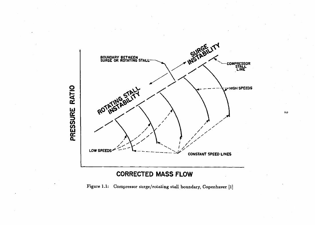
The compressor is limited by choking at higher How rates and by stall or surge at

lower flowrates. In Figure 1.1 from Copenhaver [1] is illustrated the stall-limit line

which is defined as a line that connects the compressor operating points, for different

speeds, at which stall or surge is likely to occur with any further decrease in Howrate.

Because stall and surge are aerodynamic instabilities, the stall-limit line generally

represents the boundary between stable and unstable operation of the compressor.

To avoid compressor stall or surge, a sufficient stall margin is desired. Stall margin

is a measure of how much the compressor back pressure can be increased from the

design value at a constant flow and variable speed or how much the flowrate can be

reduced from the design value at a constant speed before the compressor stalls.

The research described in this dissertation involved an effort to improve compres

sor stall margin by scheduling the blade setting angles of stationary blades upstream

of a rotor in a circumferentially periodic pattern to delay the onset of rotating stall.

Shifting the throttle line away from the stall-limit line is not generally acceptable

because of the performance penalties involved. Achieving more operating margin by

Î5 0:

UJ oc

g

S

BOUNDARY BETWEEN SURGE OR ROTATING STALL

LOW SPEEDS -

COMPRESSOR ïsy-

HIGH SPEEDS

/ /

/y'

CONSTANT SPEED LINES

to

CORRECTED MASS FLOW

Figure 1.1: Compressor surge/rotating stall boundary, Copenhaver (1]

3

shifting the stall-limit line further away from the throttle line is attractive if it can

be clone without compromising other operating characteristics of the compressor.

It is important to understand some of the physical mechanisms of stall and surge.

Stall and surge are two distinct aerodynamic flow instabilities which can occur during

the operation of a multistage compressor. Stall is generally described as the unsteady

separation of flow from blade surfaces and/or end walls resulting in rotating low-flow

or localized reversed flow regions. Rotating stall typically occurs at lower compressor

rotational speeds. Surge, in contrast, is characterized by global fluctuations in mass

flow throughout the entire compressor. Surge is generally encountered at higher

compressor rotational speeds and is easier to recover from than stall. Although these

flow instabilities are distinct, they are related. It is known that surge is generally a

result of the more localized instability of stall.

It is of great importance to compressor users to be able to understand, detect

and avoid the instabilities of stall and surge. Not only do these instabilities limit

compressor and engine performance. They can also cause damage to the compressor

blading. The unsteady nature of these instabilities leads to large periodic forces being

placed on the blades. The flow reversals associated with surge can introduce hot com

bustion gas into the compressor. Another important reason to avoid stall and surge

is that these instabilities result in significant compressor and engine performance de

terioration. The engine performance may actually fall below the level necessary to

sustain flight. In the following two sections some of the physical mechanisms of stall

and surge are described in further detail.

4

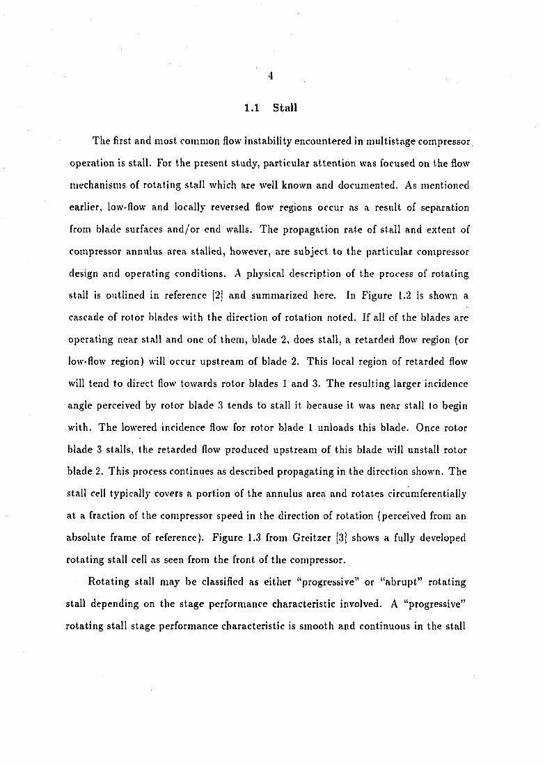
1.1 Stall

The first and most common flow instability encountered in multistage compressor

operation is stall. For the present study, particular attention was focused on the flow

mechanisms of rotating stall which are well known and documented. As mentioned

earlier, low-flow and locally reversed flow regions occur as a result of separation

from blade surfaces and/or end walls. The propagation rate of stall and extent of

compressor annulus area stalled, however, are subject to the particular compressor

design and operating conditions. A physical description of the process of rotating

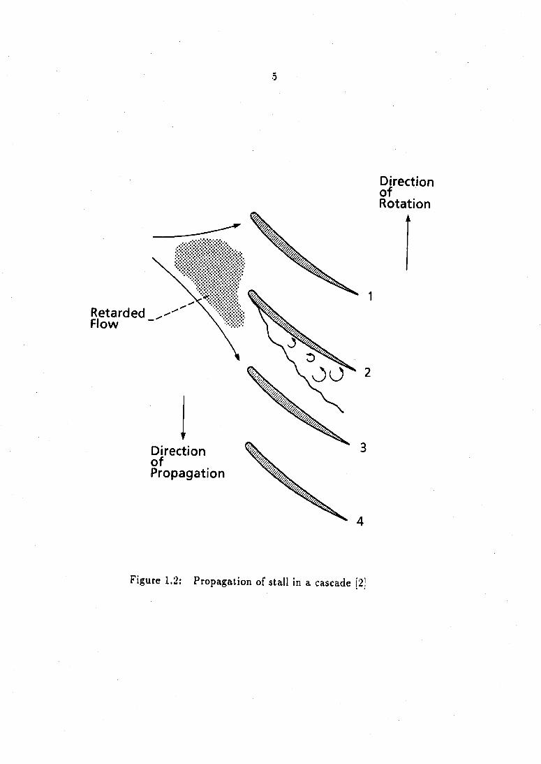
stall is outlined in reference [2] and summarized here. In Figure 1.2 is shown a

cascade of rotor blades with the direction of rotation noted. If all of the blades are

operating near stall and one of them, blade 2, does stall, a retarded flow region (or

low-flow region) will occur upstream of blade 2. This local region of retarded flow

will tend to direct flow towards rotor blades 1 and 3. The resulting larger incidence

angle perceived by rotor blade 3 tends to stall it because it was near stall to begin

with. The lowered incidence flow for rotor blade 1 unloads this blade. Once rotor

blade 3 stalls, the retarded flow produced upstream of this blade will unstall rotor

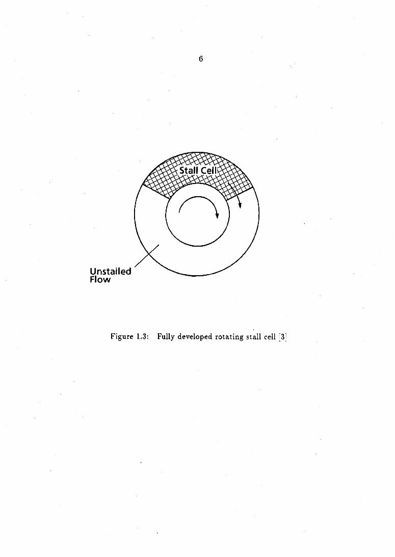
blade 2. This process continues as described propagating in the direction shown. The

stall cell typically covers a portion of the annulus area and rotates circumferentially

at a fraction of the compressor speed in the direction of rotation (perceived from an

absolute frame of reference). Figure 1.3 from Greitzer [3) shows a fully developed

rotating stall cell as seen from the front of the compressor.

Rotating stall may be classified as either "progressive" or "abrupt" rotating

stall depending on the stage performance characteristic involved. A "progressive"

rotating stall stage performance characteristic is smooth and continuous in the stall

5

Direction of Rotation

Retarded Flow

Direction of Propagation

Figure 1.2: Propagation of stall in a cascade [2]

Unstalled Flow

Figure 1.3: Fully developed rotating stall cell [31

i

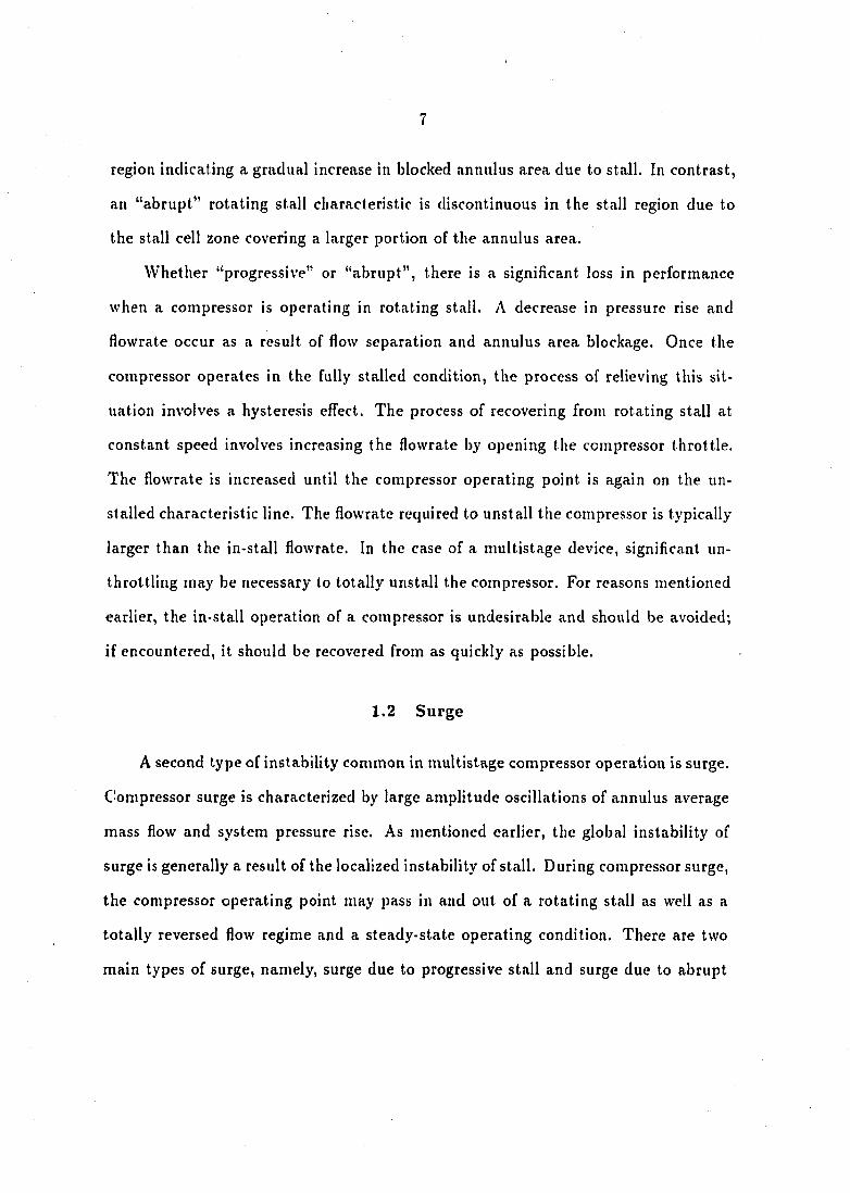
region indicating a gradual increase in blocked annulus area due to stall. In contrast,

an "abrupt" rotating stall characteristic is discontinuous in the stall region due to

the stall cell zone covering a larger portion of the annulus area.

Whether "progressive" or "abrupt", there is a significant loss in performance

when a compressor is operating in rotating stall. A decrease in pressure rise and

flowrate occur as a result of flow separation and annulus area blockage. Once the

compressor operates in the fully stalled condition, the process of relieving this sit

uation involves a hysteresis effect. The process of recovering from rotating stall at

constant speed involves increasing the flowrate by opening the compressor throttle.

The flowrate is increased until the compressor operating point is again on the un-

stalled characteristic line. The flowrate required to unstall the compressor is typically

larger than the in-stall flowrate. In the case of a multistage device, significant un-

throttling may be necessary to totally unstall the compressor. For reasons mentioned

earlier, the in stall operation of a compressor is undesirable and should be avoided;

if encountered, it should be recovered from as quickly as possible.

1.2 Surge

A second type of instability common in multistage compressor operation is surge.

Compressor surge is characterized by large amplitude oscillations of annulus average

mass flow and system pressure rise. As mentioned earlier, the global instability of

surge is generally a result of the localized instability of stall. During compressor surge,

the compressor operating point may pass in and out of a rotating stall as well as a

totally reversed flow regime and a steady-state operating condition. There are two

main types of surge, namely, surge due to progressive stall and surge due to abrupt

8

stall. Surge clue to progressive stall, is generally mild and inaudible when encountered

in multistage compressor operation. Experimental investigations indicate that this

type of surge occurs when there are no abrupt changes in the pressure ratio due to

stall. Tests indicate that the total-pressure fluctuations measured may be only 15 to

20 percent of that encountered when the compressor surges abruptly. Whereas surge

due to progressive stall is mild and inaudible, surge due to abrupt stall is violent

and very audible. In fact, certain surge cycles observed in jet engine operation can

cause flames from the combustion chamber to exit from the front of the compressor.

This situation is very undesirable. Examination of actual data indicates that large

pressure fluctuations can exist at the compressor discharge which may be up to 75

percent of the compressor pressure rise at the surge point.

The importance of detecting and avoiding stall and surge was mentioned ear

lier. When the compressor is subjected to periodic forces as a result of rotating

stall or surge, a significant loss in performance is realized and blade failure may oc

cur. In general, avoiding these instabilities, or if encountered, recovering quickly, are

worthwhile objectives. In the following section, some of the current methods being

investigated to avoid stall or surge, including extending the useful operating range of

the compressor are considered.

1.3 Avoiding Stall

Current methods for avoiding stall or surge can be broken down into two major

categories, static control and active control. Some static control methods for avoiding

stall include designing blades with a higher tolerance to stall (higher diffusion limits),

using boundary layer control methods such as vortex generators, suction, and blowing,

9

and using casing treatments, and using existing control variables such as compressor

rotational speed and mass flow. Active control of rotating stall involves utilizing a

feedback control loop coupled to a variable geometry feature of the compressor to

avoid or recover from stall.

Static control methods for avoiding stall are somewhat limited as compared to

active control methods for improving the useful operating range of the compressor.

.A.lthough blades are being designed with a higher tolerance to stall, improvements in

design cannot satisfy increased demands associated with improved compressor stall

resistance. The static methods using boundary layer control have also enjoyed limited

success only because the boundary layer cannot be altered enough. The final method

of static control, varying compressor rotational speed and flowrate, is also very limited

in its scope as a potential for avoiding stall. During compressor operation, the rota

tional speed and flowrate are often set parameters which cannot be altered quickly

enough to reach a more stable operating point. The active methods of avoiding stall

and surge have been significantly more successful in controlling these instabilities and

extending the useful operating ranges of compressors. A. H. Epstein, a professor of

Aeronautics and .'Astronautics at MIT, envisions a multistage compressor in which

there is a microprocessor in every blade [4]. Commonly known as "smart" engine

technology, the idea is that the microprocessor senses local flow conditions (veloc

ity, pressure, etc.) and sends a feedback control signal to a computer processor. If

the local flow conditions indicate that an instability is about to occur, the computer

processor will send a signal to actuate some variable geometry feature of the com

pressor to avoid the instability. Some possible variable geometry features that have

been considered are bleed doors, adjustable inlet guide vanes and stators, flaps on

10

inlet guide vanes, and even recamberable blades. Although these variable geometry

features can add weight to the compressor, the trade-off in improved performance

and stability make them attractive.

The proposed method for improving the stall margin of a multistage, axial-flow

compressor considered in this dissertation is classified as a static method which could

become a component of an active system. The method utilizes a circumferential

variation of stationary blade setting angles to create a specific flowfield variation for

the downstream rotor. The method is based on airfoil dynamic stall results which

suggest that an airfoil oscillating about an axis perpendicular to the blade section can

achieve angles of attack (average and instantaneous) that are higher than its static

stall angle of attack. When the blade is oscillated at certain angle amplitudes and

frequencies, its dynamic stall angle of attack may be as much as 20 percent higher

than its static stall angle of attack. The intent of the circumferential variation in

stationary blade setting angles is to produce a flowfield for the downstream rotor

blades that is similar to the flowfield of an oscillating airfoil. By making the rotor

flowfield similar to that of an oscillating airfoil, the rotor is expected to achieve higher

instantaneous and average angles of attack before stalling. The higher angles of attack

achieved allow the rotor to be loaded more without stalling and thus previously

unattainable low flowrates can be realized before stall occurs. This reduction in

the compressor flowrate before stall occurs corresponds to an increase in the useful

operating range of the compressor and thus stall margin which is the intent of the

method. In the following chapter airfoil dynamic stall research and how it can be

extended to multistage, axial-flow compressor operation is discussed. Some possible

11

limitations associated with extending dynamic stal research concepts to compressor

operation are also outlined.

2. RELATED ISOLATED AIRFOIL DYNAMIC STALL RESEARCH

The idea for modifying the stall margin of axial-flow compressors by circum-

ferentially varying the setting angles of stationary blades upstream of a rotor stems

from airfoil dynamic stall research. Dynamic stall research involves studies performed

on airfoils pitching harmonically about an axis perpendicular to the blade section.

Helicopter rotor blade development has led to several airfoil dynamic stall studies

(hat suggest that a pitching blade, whose setting angle is varied periodically over a

range of values, is able to sustain without stalling, angles of attack (instantaneously

and on an average basis) that are larger than the static (stationary blade) stall angle.

The increased stalling angle (average) of the airfoil can be credited to the oscillatory

nature of the airfoil. The basic idea is that although the blade becomes highly loaded

as it periodically cycles to an angle greater than the static stall angle, it is subse

quently relieved as it moves to angles less than the static stall angle. Results show

that this increased stalling angle (average), also called the dynamic stall angle, may

be as high as 20 percent greater than the static stall angle of attack.

For an axial-flow compressor to benefit from the dynamic stall effect, the flowfield

for the rotor blade must be made similar to that of a harmonically oscillating airfoil.

An attempt at accomplishing this is done by repositioning upstream stationary blade

setting angles in a periodic pattern around the circumference. As the rotor blade

13

rotates around the circumference, it sees a varying relative angle of attack which is

similar to the varying angle of attack that a pitching airfoil sees. The angle amplitude

and frequency of the setting angle variation upstream results in a predetermined

change in relative angle of attack and frequency of variation perceived by the rotor.

The concept described for improving the stall margin of axial-flow compressors

using the dynamic stall effect is simplistic in that it does not account for possible

differences existing between the two flowfields. Dynamic stall studies are largely

two-dimensional flow studies performed on simple airfoil geometries with negligible

three-dimensional flow effects. These three-dimensional efl'ects are very much present

in the complex flowfleld of a compressor and they determine the performance of

the compressor. Additional compressor efl'ects not fully addressed by dynamic stall

studies are the eff^ects of increasing Mach number and lowering blade aspect ratio.

Regardless of the differences which may exist in the two flowfields, dynamic stall

studies lead to some important ideas that are worth examining.

From a two-dimensional standpoint, some of the important factors affecting the

dynamic stall angle are:

1. Rate of airfoil oscillation

2. Amplitude of airfoil oscillation

3. Airfoil geometry

4. Airfoil Mach number

Perhaps the most important factor listed is the rate at which the airfoil pitches.

The rate at which the airfoil pitches is usually non-dimensionalized and called the

reduced frequency, K. The reduced frequency represents the ratio of the time required

14

for the fluid to pass over one-half blade chord to the time period of pitching motion

of the airfoil. The reduced frequency is defined as follows:

It is noteworthy that as K — 0, the airfoil oscillation rate approaches the static

limit (stationary airfoil) and the effect of oscillation is negligible.

The selection of the proper reduced frequency to use in the low-speed compressor

tests was guided by data presented in some of the isolated airfoil dynamic stall studies.

In Figure 2.1 is depicted a typical airfoil pitching about a midchord axis with some

of the important parameters associated with airfoil dynamic stall studies noted.

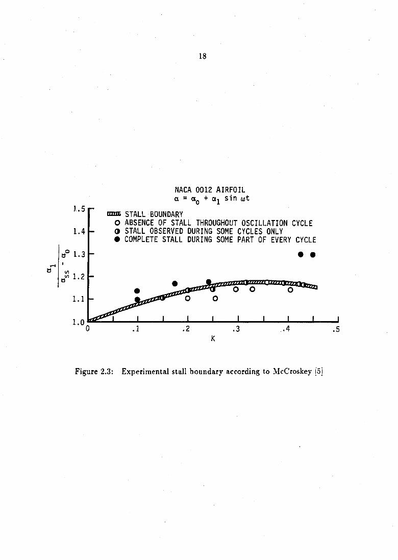
The two-dimensional pitching airfoil data presented by McCroskey [5] indicate

that the extent by which the static stall angle can be exceeded by an airfoil pitching

angle amplitude without dynamic stall occurring increases with increased reduced

frequency, reaching a maximum in the range of K from 0.30 to 0.35. In that study,

an NACA 0012 airfoil was oscillated in pitching motion as indicated by the equation:

(2 .1)

where

/ = frequency of pitching motion of dynamic stall airfoils

c = airfoil chord length

V = representative freest ream speed of fluid past the airfoil

Q = Qo + «isin (2.2)

where

Q = instantaneous angle of attack

Oo = angle about which the airfoil pitches

1.5

Figure 2.1: Typical airfoil pitching about a midchorcl axis

16

ai = amplitude of angle variation

w = rate of airfoil pitching, u> = 27r/

t = time

The three parameters: ao, angle about which the airfoil pitches; ai, amplitude

of angle variation; and w, rate of airfoil pitching, were varied over a range of values

in an attempt to construct the experimental stall boundary for the NACA 0012

airfoil. In Figure 2.2 is a sketch of the airfoil geometry and some of the important

angular positions associated with these tests. The data of Figure 2.3, including the

experimental stall boundary, illustrate the extent by which the static stall angle can

be exceeded without dynamic stall occurring anywhere in the cycle. The angle a,,

represents the angle of attack for which static stall was observed. Thus, ^ is the

amount by which the airfoil is oscillated past the static stall position, as illustrated in

Figures 2.2 and 2.3. The open symbols denote absence of stall throughout the cycle,

half-solid symbols denote test points for which stall was observed during some cycles

and not during others, and the solid symbols denote complete stall during some part

of every cycle. The resulting experimental stall boundary suggests that the delay of

stall increases with reduced frequency, reaching a maximum in the range of reduced

frequency. A', from 0.30 to 0.35. With further increases in the reduced frequency, no

additional delay of stall was noticed.

The pitching airfoil data presented by Halfman, Johnson, and Haley [6] seem

to verify and extend the results presented by McCroskey [5). In their study, three

different airfoil geometries (blunt, sharp, and intermediate wings) were oscillated in

pitching motion as indicated by Equation (2.2). In their study, Halfman et al. per

formed tests at a constant amplitude of oscillation, ai, of 6.08°, and varied the

17

ss

Figure 2.2: .Airfoil geometry and important angular quantities. McCroskey 5!

18

1.5

1.4

NACA 0012 AIRFOIL a = ttg + oj sin tot

nna STALL BOUNDARY O ABSENCE OF STALL THROUGHOUT OSCILLATION CYCLE O STALL OBSERVED DURING SOME CYCLES ONLY • COMPLETE STALL DURING SOME PART OF EVERY CYCLE

1.2

Figure 2.3: Experimental stall boundary according to McCroskey [Sj

19

parameters «g and K to determine the extent by which the static stall angle could

be exceeded at various reduced frequencies. In addition, they also performed tests at

different Aa values, where

Aa = «0 - fVij (2.3)

In their report, Halfman et al. described the increase in the dynamic stall angle by

the quantity:

5a = attaii - (2.4)

where

= instantaneous stall angle of attack

= static stall angle of attack

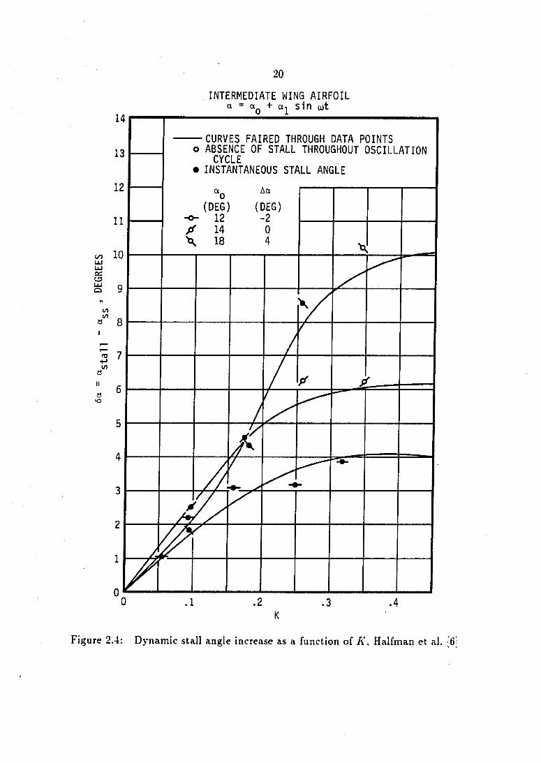
The data in Figure 2.4 show the results of tests performed on the intermediate

wing airfoil geometry and is a plot of 6a versus the reduced frequency, A', for three

different values of Aa (—2°, 0°, and 4°). The solid symbols denote the instantaneous

angle of attack for which the intermediate wing stalled. The instantaneous stalling

angle was determined from traces of the variation of moment in pitch throughout

a cycle of oscillation and corresponds to the angle of attack at which the moment

drops sharply. The open symbols indicate "no stall" occurring throughout the cycle

of oscillation. The solid lines are curves that are faired through the data points for Aa

values of —2°, 0°, and 4°. Additional plots showing similar trends were constructed

by Halfman et al. for the remaining two wing airfoil geometries, blunt and sharp

wings, but are not included here. It is evident from the information of Figure 2.4

that the quantity 6a increases with larger reduced frequency and reaches a maximum

in the range of A' from 0.30 to 0.35, depending on the particular value of Aa. In

20

00

C3

(/)

0 1

m 4-» CO

a II

a LO

INTERMEDIATE WING AIRFOIL a = a. + a, sin lut

CURVES FAIRED THROUGH DATA POINTS o ABSENCE OF STALL THROUGHOUT OSCILLATION

CYCLE • INSTANTANEOUS STALL ANGLE

OQ Act

(DEG) (DEG) -o- 12 -2 X 14 0 \ 18 4 ta

/ /

/ f

/ X

f /

. 1 . 2 .3 .4

Figure 2.4: Dynamic stall angle increase as a function of A', Halfman et al. '6!

21

fact, the data point corresponding to tSa = 10° and K = 0.35 for Aa = 4° involved

no evidence of stall anywhere in the cycle. Thus, in tests where the intermediate

wing airfoil oscillated about a nominal angle of attack («(,) 4° above its static stall

angle of attack (a„) with a pitching angle amplitude (aj ) of 6.08°, the airfoil showed

no signs of stalling anywhere in the cycle at a reduced frequency, K = 0.35. This

observation leads to the conclusion that a pitching airfoil can sustain average as well

as instantaneous angles of attack that are larger than the static stall angle of attack

at certain amplitudes of oscillation and reduced frequencies.

The studies performed on simple two-dimensional airfoil geometries by Mc-

Croskey [5] and Halfman et. al. [6] suggest that the maximum delay of stall occurs

at a reduced frequency, A', in the range from 0.30 to 0.35. This range of reduced

frequency was considered when initial attempts were made for improving the stall

margin of two low-speed compressors.

Another parameter affecting the extent to which airfoils experience the dynamic

stall phenomena is the amplitude of pitching motion, ai of Equation (2.2). Accord

ing to McCroskey, Carr, and McAlister [7], the amplitude of pitching motion, Oj,

generally determines the characteristics of the time dependent aerodynamic forces

and moments for a pitching airfoil. McCroskey further states that these aerodynamic

quantities may be considerably larger and different in nature from their steady-state

counterparts. Because the dynamic stall angle is usually determined from time de

pendent aerodynamic force and moment traces, the amplitude of pitching motion is

very important. Past pitching airfoil experiments were performed over a wide range

of pitch angle amplitudes. McCroskey [5] performed tests on an oscillating NAC.A

0012 airfoil section with a 4° to 19° range of pitching motion angle amplitude. Later,

22

McCroskey et al. [7| used an angle amplitude range of 6° to 14°. Experiments per

formed on different airfoil sections by Halfman et al. [6] were pitched at a constant

angle amplitude of 6.08°. Other tests by McCroskey and Pucci [8] involved a .5°

angle amplitude, while Liiva [9) performed tests with angle amplitudes in the range

from 2.5° to 7..5°. The wide range of amplitudes of pitching motion mentioned in the

studies cited above can be attributed to attempts by the authors involved to identify

some of the stalling characteristics of pitching airfoils for different airfoil geometries.

These values of pitching motion amplitude were considered in selecting the proper

amplitude of blade setting angle variations for the low-speed compressor tests.

.Another important feature affecting the increased stall angle of harmonically

pitching airfoils is the airfoil geometry. Halfman et al. [6] concluded that the airfoil

shape primarily affects the suddenness and type of flow separation under dynamic

stalling conditions. Similarly, McCroskey et al. [7] and McCroskey and Pucci [8]

stated that airfoil leading edge geometry has a strong affect on the type of boundary-

layer separation that occurs. Liiva [9] contended that a cambered airfoil has better

aerodynamic characteristics under dynamic stalling conditions because the adverse

pressure gradient is decreased by nose camber. It is expected that the airfoil geometry

as well as the compressor geometry will be important in determining the success of

the method outlined for improving the stall margin of compressors. Simple two-

dimensional airfoils sustaining increased angles of attack does not necessarily mean

that a compressor rotor may achieve this as well. Further, as the rotational speed

(and thus Mach number) increases, so does the effect of geometry on the overall

performance of the compressor. For the low-speed compressor tests, the rotor of the

two-stage axial-flow fan had minimal nose camber, while the British C4 section rotor

23

blades of the three-stage axial-flow compressor involved substantial nose camber.

The remaining parameter affecting dynamic stall is airfoil Mach number. The

major effect of Mach number on the stalling characteristics of a harmonically pitching

airfoil are leading edge effects and the corresponding separation type as mentioned

by McCroskey and Pucci [8] and Liiva [9]. As with airfoil and compressor geometry,

the Mach number is expected to be an important factor in the success of the method

outlined in this dissertation. It may be that the effect of increasing Mach number in

a compressor degrades the increased stalling angle found in the dynamic stall phe

nomena. Typical Mach numbers evaluated at the design point operating conditions

for the two-stage fan and three-stage compressor were near 0.10. The Mach numbers

associated with the stalling condition of the Pratt & Whitney compressor varied with

rotational speed and were in the range from 0.08 to 0.21.

3. PROOF OF CONCEPT IN LOW-SPEED COMPRESSORS

The following chapter describes experimental tests performed at Iowa State Uni

versity on two low-speed compressors, namely a two-stage, axial-flow fan and a three-

stage, axial-flow compressor. These tests were used as a preliminary step in evaluat

ing the potential for using circumferentially varying stationary blade setting angles

to improve compressor stall margin. Descriptions of the two compressors, related

equipment, experimental procedures and results are presented. This chapter also

presents some detailed measurements taken with the three-stage compressor. The

detailed measurements (flow angle and magnitude) were performed behind the inlet

guide vanes of the baseline compressor configuration as well as some modified com

pressor configurations. These measurements provided additional information about

the flowfleld being produced by the blade setting angle variation upstream. Using

the detailed flow information, comparisons were made between the estimated and

actual reduced frequencies and rotor inlet flow angle variations for the low-speed

compressor. The analysis of this preliminary work guided further attempts with an

intermediate-speed, three-stage, axial-flow compressor.

25

3.1 Stationary Blade Setting Angle Variations

The main research objective was to determine the influence on stall point of

circumferential variations of stationary blade setting angles involving different re

duced frequencies and amplitudes of rotor inlet flow angle variation. Blade setting

angle patterns could be changed easily in the two-stage fan and three-stage compres

sor. These pattern changes were not as easily accomplished in the Pratt & Whitney

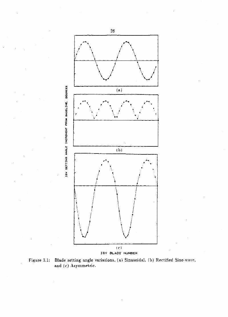
compressor because of its complexity. Three different blade setting angle variation

patterns were evaluated in tests. These patterns consisted of sinusoidal, rectified

sine-wave, and asymmetric variations of angles and are illustrated in Figure .3.1. The

equations describing these angle schedules are given below;

Sinusoidal Variation:

Pi = individual blade setting angle

4>o = baseline blade setting angle

Ap = amplitude of blade setting angle circumferential variation

n = number of setting angle variation cycles per rotor revolution

N = number of blades in stationary row

i — individual blade number

(3.1)

where

Rectified Sine-wave Variation:

4>i =(}>„ + Ùk4> sin (i - 1) (3.2)

where the parameters are explained above.

26

a Ui OC

(a )

d i U z H K N > 19

I c) IGV BLADE NUMBER

Figure 3.1: Blade setting angle variations, (a) Sinusoidal, (b) Rectified Sine-wave, and (c) .Asymmetric.

27

Asymmetric Variation:

(i)o + Mism - 1)J for , = 1.10,20-28

0,, +A^2sin[^(;-1)] for i=l 1-19,29-37 (3.3)

where and Aéo different amplitudes of blade setting angle circumferential

variation and the number of setting angle variation cycles per rotor revolution, n,

was set at 2, for 37 blades in a stationary row.

The two-stage fan tests involved only sinusoidal variations in blade setting angle

while during the three-stage compressor tests, all three kinds of variations in blade

setting angle were used. The Pratt & Whitney compressor tests were accomplished

with only one asymmetric variation in blade setting angle.

The intent of the circumferential variations in stationary blade setting angle was

to create a variation in inlet flow angle amplitude and frequency for a downstream

rotor blade row. The amplitude of setting angle variation, Aip, resulted in a specific

rotor inlet flow angle variation and the number of setting angle variation cycles per

rotor revolution, n, gave the frequency of the variation. The frequency of the peri

odic variation imposed on each downstream rotor blade was given by the following

equation

n { R P M )

60 (3.4)

where

/ = frequency of circumferentially periodic setting angle variation

n = number of setting angle variation cycles per rotor revolution

RPM = rotor rotational speed

Substituting Equation (2.1) into Equation (3.4) and rearranging gives an estimate for

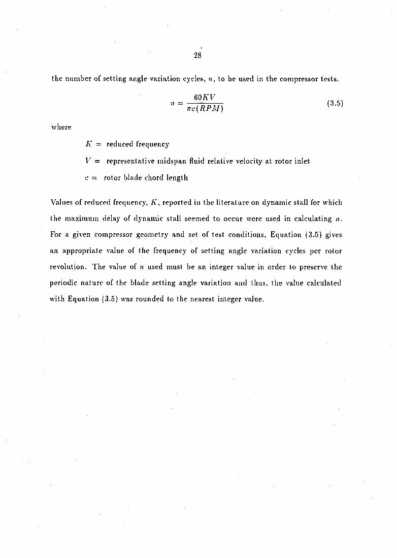
28

the number of setting angle variation cycles, ri, to be used in the compressor tests.

60 Al/ " ~ 7VC(RPM) ( ' )

where

K — reduced frequency

I = representative midspan fluid relative velocity at rotor inlet

c = rotor blade chord length

Values of reduced frequency, A", reported in the literature on dynamic stall for which

the maximum delay of dynamic stall seemed to occur were used in calculating ri.

For a given compressor geometry and set of test conditions, Equation (3.5) gives

an appropriate value of the frequency of setting angle variation cycles per rotor

revolution. The value of n used must be an integer value in order to preserve the

periodic nature of the blade setting angle variation and thus, the value calculated

with Equation (3.5) was rounded to the nearest integer value.

29

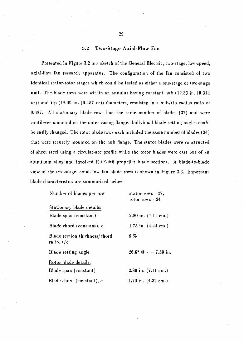
3.2 Two-Stage Axial-Flow Fan

Presented in Figure 3.2 is a sketch of the General Electric, two-stage, low-speed,

axial-flow fan research apparatus. The configuration of the fan consisted of two

identical stator-rotor stages which could be tested as either a one-stage or two-stage

unit. The blade rows were within an annulus having constant hub (12.36 in. (0.314

m)) and tip (18.00 in. (0.457 m)) diameters, resulting in a hub/tip radius ratio of

0.687. .All stationary blade rows had the same number of blades (37) and were

cantilever mounted on the outer casing flange. Individual blade setting angles could

be easily changed. The rotor blade rows each included the same number of blades (24)

that were securely mounted on the hub flange. The stator blades were constructed

of sheet steel using a circular-arc profile while the rotor blades were cast out of an

aluminum alloy and involved RAF-#6 propeller blade sections. A blade-to-blade

view of the two-stage, axial-flow fan blade rows is shown in Figure 3.3. Important

blade characteristics are summarized below:

Number of blades per row stator rows - 37, rotor rows - 24

Stationary blade details:

Blade span (constant)

Blade chord (constant), c

Blade section thickness/chord ratio, t/c

Blade setting angle

Rotor blade details:



2.80 in. (7.11 cm.)

1.70 in. (4.32 cm.)

26.0° @ r = 7.59 in.

2.80 in. (7.11 cm.)

1.75 in. (4.44 cm.)

6 %

5.4m

7-1/2 HP DYNAMOMETER

AIR STRAIGHTENING TUBES THROTTLE CONE FAN INLET TWO-STAGE FAN

0.864m

Figure 3.2: Two-stage axial-flow fan apparatus

31

Blade section maximum thickness/ 12 % chord ratio, t,„ar/c

Blade setting angle 65.0° @ r = 7.59 in.

The two-stage, axial-flow fan was driven by a HP cradled D.C. dynamome

ter. Variable voltage control for the dynamometer was provided by a General Elec

tric speed variat or which permitted testing within a range of shaft speed from 500

rpm minimum to 3000 rpm maximum. Rotor speed was measured with a frequency

counter mounted on the dynamometer shaft. .A. General Electric voltage variac was

added to the control circuitry of the GE speed variator to enable the rotor speed to

be adjusted and held constant to within ± 2 rpm. Rotational speed was measured

with a frequency counter mounted on the dynamometer shaft. Further details about

the two-stage, low-speed, axial-flow fan may be found in reference [10].

3.2.1 Two-stage fan performance tests

With the two-stage fan, one-stage and two-stage overall performance tests involv

ing different circumferential variations of stator blade setting angles were performed

at shaft speeds of 2000 rpm and 1600 rpm, respectively. Circumferential variations in

stationary blade setting angle set in the two-stage fan builds involved resetting both

stationary rows of the fan with identical blade setting angle variations. The stator

rows were aligned axial I y so that the identical variations were in phase geometrically.

The overall performance characteristics of the fan, namely, fan head-rise and

flowrate, were measured and non-dimensionalized into the total-head rise coefficient

and flow coefficient shown in Equations (3.6) and (3.7). The fan head-rise was mea

sured with a wall static pressure ring located one fan diameter downstream of the

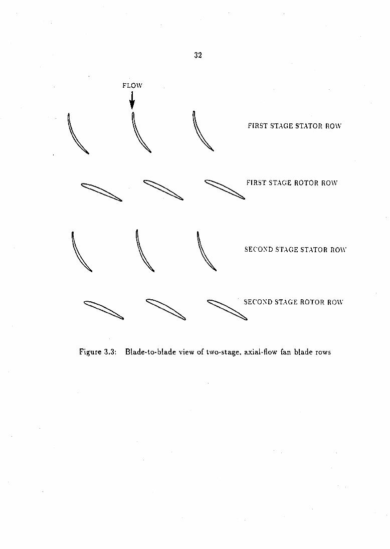
FLOW

I

32

FIRST STAGE STATOR ROW

FIRST STAGE ROTOR ROW

SECOND STAGE STATOR ROW-

SECOND STAGE ROTOR ROW

Figure 3.3: Blade-to-blade view of two-stage, axial-flow fan blade rows

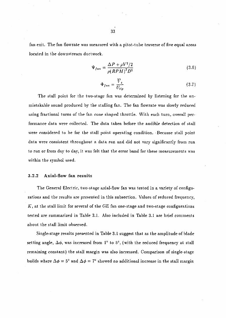
33

fan exit. The fan How rate was measured with a pitot-tube traverse of five equal areas

located in the downstream ductwork.

The stall point for the two-stage fan was determined by listening for the un

mistakable sound produced by the stalling fan. The fan Howrate was slowly reduced

using fractional turns of the fan cone shaped throttle. With each turn, overall per

formance data were collected. The data taken before the audible detection of stall

were considered to be for the stall point operating condition. Because stall point

data were consistent throughout a data run and did not vary significantly from run

to run or from day to day, it was felt that the error band for these measurements was

within the symbol used.

3.2.2 Axial-fiow fan results

The General Electric, two-stage axial-flow fan was tested in a variety of configu

rations and the results are presented in this subsection. Values of reduced frequency,

A', at the stall limit for several of the GE fan one-stage and two-stage configurations

tested are summarized in Table 3.1. .41 so included in Table 3.1 are brief comments

about the stall limit observed.

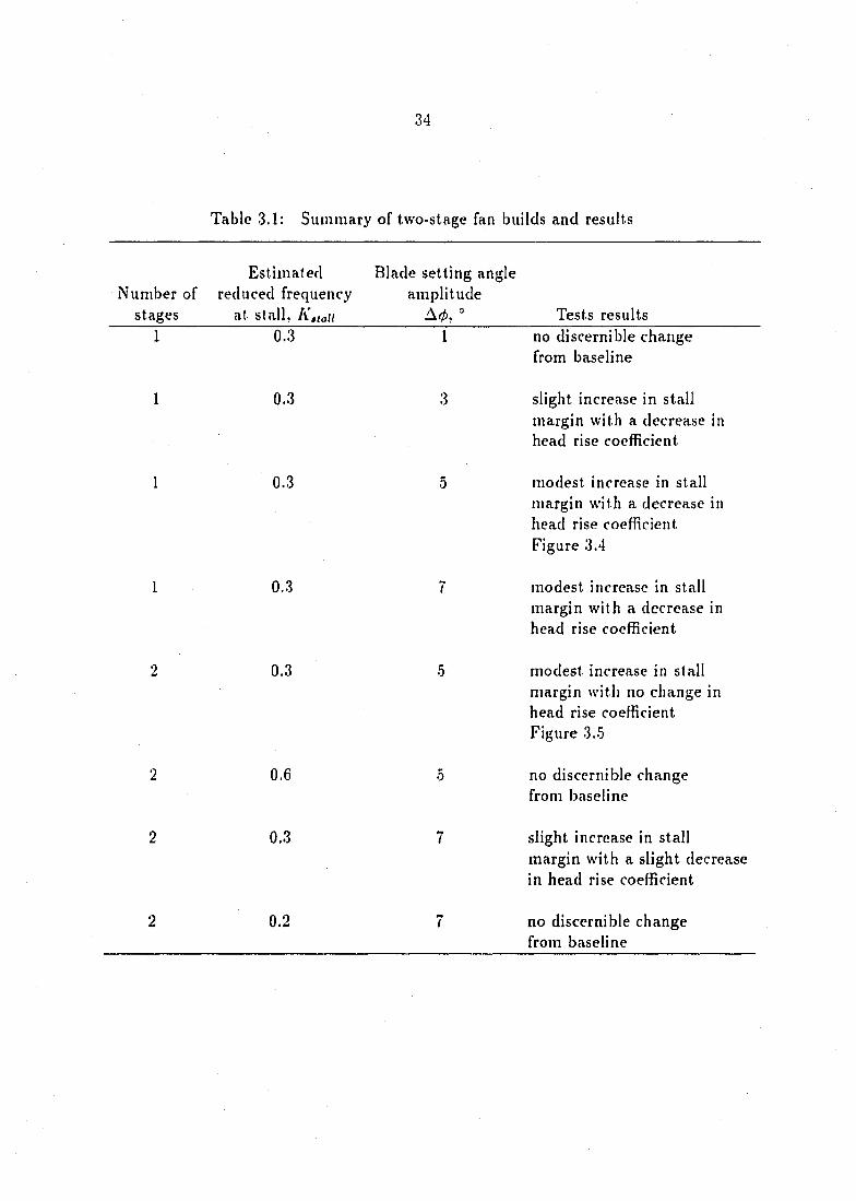
Single-stage results presented in Table 3.1 suggest that as the amplitude of blade

setting angle, was increased from 1° to 5°, (with the reduced frequency at stall

remaining constant) the stall margin was also increased. Comparison of single-stage

builds where = 5° and A(/> = 7° showed no additional increase in the stall margin

p { R P M ] ' D ' ' (3.6)

1/= (3.7)

34

Table 3.1: Summary of two-stage fan builds and results

Number of stages

Estimated reduced frequency

at stall, Kstall

Blade setting angle amplitude

Tests results 1 0.3 1 no discernible change

from baseline

1 0.3 3 slight increase in stall margin with a decrease in head rise coefficient

1 0.3 5 modest increase in stall margin with a decrease in head rise coefficient Figure 3.4

I 0.3 7 modest increase in stall margin with a decrease in head rise coefficient

2 0.3 5 modest increase in stall margin with no change in head rise coefficient Figure 3..5

2 0.6 5 no discernible change from baseline

2 0.3 7 slight increase in stall margin with a slight decrease in head rise coefficient

2 0.2 7 no discernible change from baseline

35

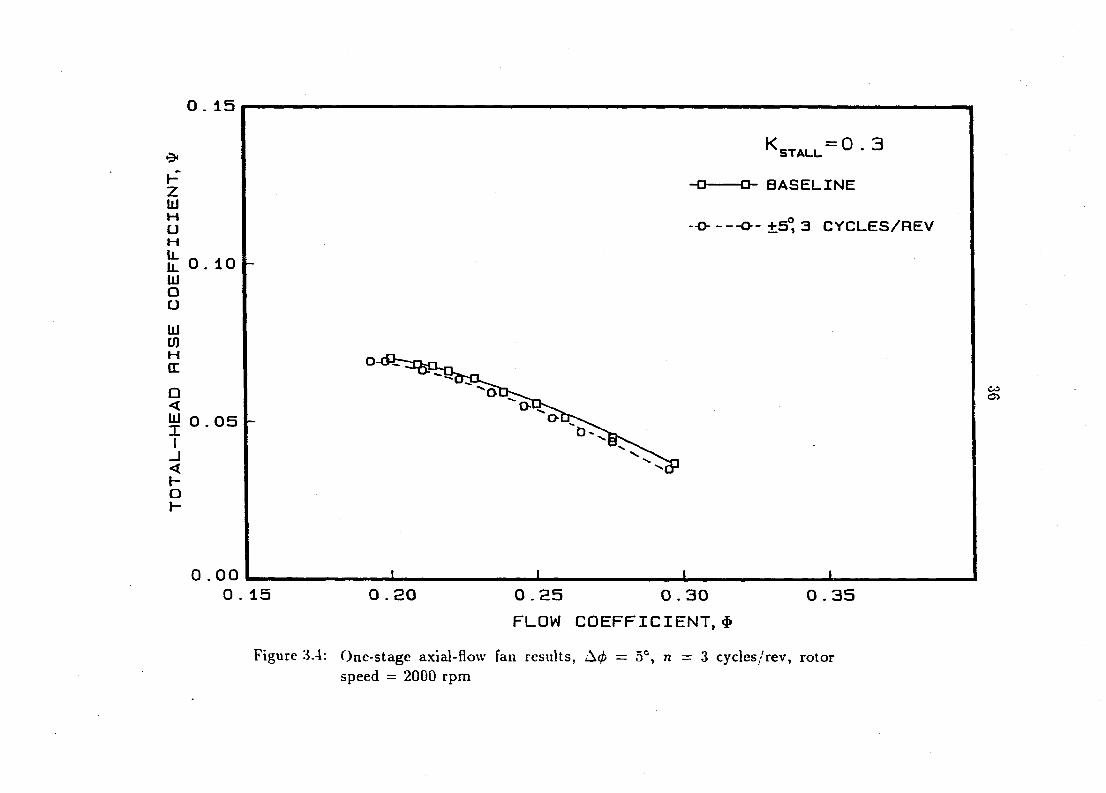
suggesting that an optimum blade setting angle amplitude was reached. Shown in

Figure 3.4 is a comparison of one-stage baseline performance and modified compressor

performance in which a sinusoidal variation in blade setting angle was used. The

modified performance shows a slight drop in head rise but also an increase in stall

margin. This increase in stall margin was modest at best but was very repeatable.

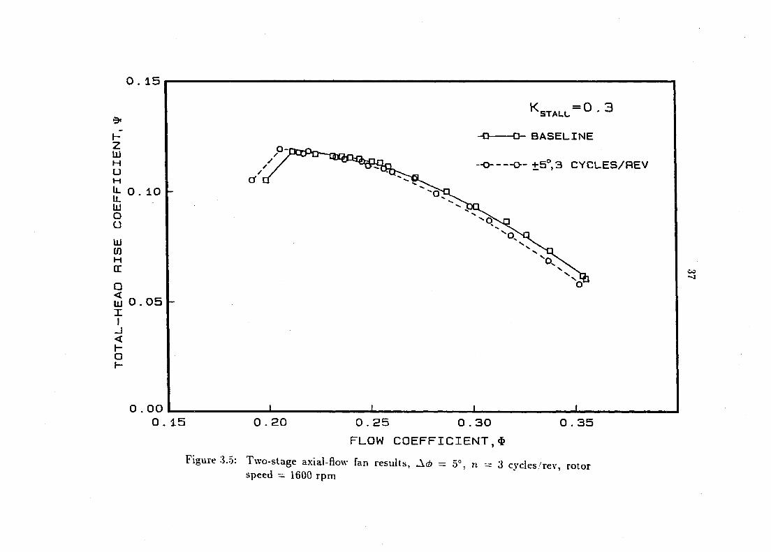
Two-stage fan tests proceeded with the amplitude of setting angle variation set

in the range of optimum results seen with the one-stage variations. A comparison

of data for two-stage builds involving a reduced frequency at stall held constant

at a value of 0.3 and the blade setting angle amplitudes varying from 5° to 7°,

suggests a decrease in stall margin with an increase in angle amplitude. Results

of Table 3.1 also suggest that when the reduced frequency was doubled to 0.60 or

reduced to 0.20 no additional increase in stall margin was noticed. This indicated

that the optimum reduced frequency was near a value of 0.30. Shown in Figure

3.5 is a comparison between two-stage baseline compressor and modified compressor

performance in which a sinusoidal variation in blade setting angle was used, The

figure illustrates the improvement in stall margin with no degradation in overall

compressor head-rise. .Again, the improvement in stall margin was modest but very

repeatable.

The results obtained by simple tests performed on the one-stage and two-stage

configurations of the GE axial-flow fan led to some important observations. The

relative magnitude of stall margin increase seemed to be most noticeable when the

reduced frequency value at stall, K,taih was near 0.3 and the stator blade setting angle

amplitude, Ù0, was in the range from 5° to 7°. Further, because of the small differ

ences in performance involved it was important to confirm all results by repeating

0 . 15

h-Z UJ H u M

t 0. 10 UJ 0 u

lU U) H Œ

• < ^ 0 . 0 5

1 _l < H O H

0 . 0 0

^ STALL ^ ^

-a- BASELINE

O O- +5° 3 CYCLES/REV

CO O

± 0 . 1 5 0 . 2 0 0 . 2 5 0 . 3 0

FLOW COEFFICIENT, $

0 .35

Figure 3.4; One-stage axial-How fan results, = 5°, n = 3 cycles/rev, rotor speed = 2000 rpm

0 . 15

9"

H Z lU H U M U_ 0 . 10 U. UJ o u

UJ tn H Œ

• < UJ 0 . 05 I 1 1 _J < H O H-

0 . 00

K STAUU= 0 - 3

-o- BASELINE

-O O- +5°, 3 CYCLES/REV

± 0 . 1 5 0 . 2 0 0 . 2 5 0 . 3 0 0 . 3 5

FLOW COEFFICIENT,$

Figure 3.5: Two-stage axial-flow fan results, Aé = 5°, n 3 cycles rev, rotor speed — 1600 rpm

38

tests several times. Finally, the benefit of multistage operation is shown by compar

ing one-stage and two-stage fan tests. Test results suggest that the loss in head-rise

is more pronounced for the one-stage fan tests than the two-stage fan tests. The stall

margin increases for the two-stage configurations seemed to be slightly higher than

those for the one-stage configurations.

39

3.3 Three-Stage Axial-Flow Compressor

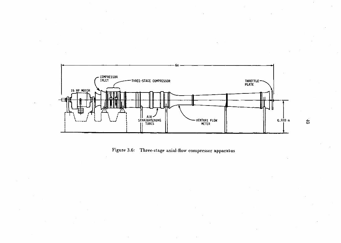
In Figure 3.6 is a sketch of the three-stage, low-speed, axial-flow compressor

apparatus used in the experimental investigation. A smooth gradually contracting

inlet to the compressor guided the flow entering the inlet guide vane (IGV) row and

three downstream sets of rotor-stator stages. A blade-to-blade view of the three-

stage, axial-flow compressor blade rows is shown in Figure 3.7. The IGV row and

the three identical rotor-stator stages were within an annulus having constant hub

(11.22 in. (0.28.5 /j?)) and tip (16.00 in. (0.406 m)) diameters, resulting in a hub/tip

radius ratio of 0.702. .All stationary blade rows had the same number of blades

(37). These blades were cantilever mounted from the outer annulus wall on separate

ring assemblies which could be moved circumferentially either independently or in

groups. The rotor blade rows each included the same number of blades (38) that

were attached on rings on a common drum with corresponding blade stacking axes

aligned axially. .All of the blades were constructed of a plastic material (Monsanto

ABS) with British C4 sections stacked to form a free vortex design.

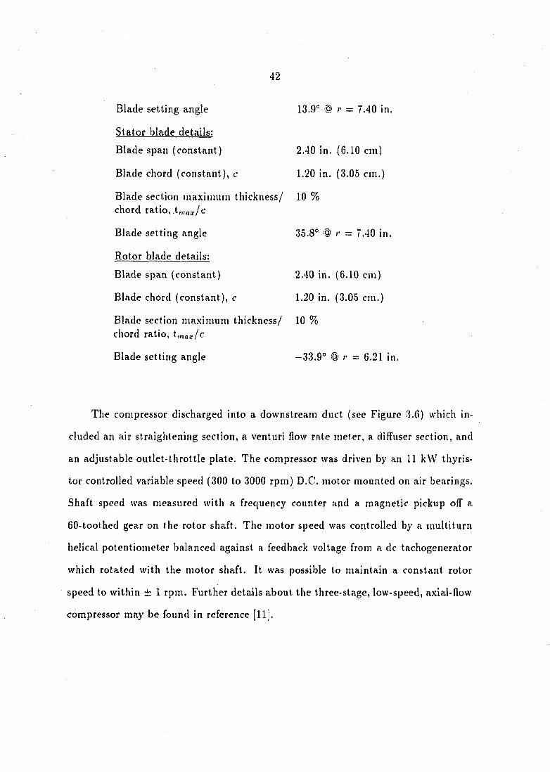
Overall blade characteristics for the three-stage, low-speed, axial-flow research

compressor are summarized below:

Number of blades per row IGV and stator rows - 37, rotor rows - 38

IGV blade details:



2.40 in. (6.10 cm)

1.20 in. (3.05 cm.)

Blade section maximum thickness/ 10 % chord ratio, t^ax/c

THROTTLE PLATE

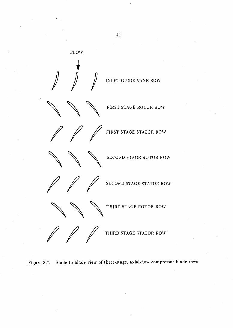
41

FLOW

i

^ INLET GUIDE VANE ROW

FIRST STAGE ROTOR ROW

FIRST STAGE STATOR ROW

SECOND STAGE ROTOR ROW

SECOND STAGE STATOR ROW

THIRD STAGE ROTOR ROW

THIRD STAGE STATOR ROW

Figure 3.7: Blade-to-blade view of three-stage, axial-flow compressor blade rows

42

Blade setting angle 13.9° @ ;• = 7.40 in.

Stator blade details:

Blade span (constant) 2.40 in. (6.10 cm)

Blade chord (constant), c 1.20 in. (3.05 cm.)

Blade section maximum thickness/ 10 % chord ratio, ,t,nar/c

Blade setting angle 35.8° # r = 7.40 in.

Rotor blade details:

Blade span (constant) 2.40 in. (6.10 cm)

Blade chord (constant), c 1.20 in. (3.05 cm.)

Blade section maximum thickness/ 10 % chord ratio, imaxlc

Blade setting angle —33.9° '§> r = 6.21 in.

The compressor discharged into a downstream duct (see Figure 3.6) which in

cluded an air straightening section, a venturi flow rate meter, a diffuser section, and

an adjustable outlet-throttle plate. The compressor was driven by an 11 kW thyris-

tor controlled variable speed (300 to 3000 rpm) D.C. motor mounted on air bearings.

Shaft speed was measured with a frequency counter and a magnetic pickup off a

60-toothed gear on the rotor shaft. The motor speed was controlled by a multiturn

helical potentiometer balanced against a feedback voltage from a dc tachogenerator

which rotated with the motor shaft. It was possible to maintain a constant rotor

speed to within ± 1 rpm. Further details about the three-stage, low-speed, axial-flow

compressor may be found in reference [11].

43

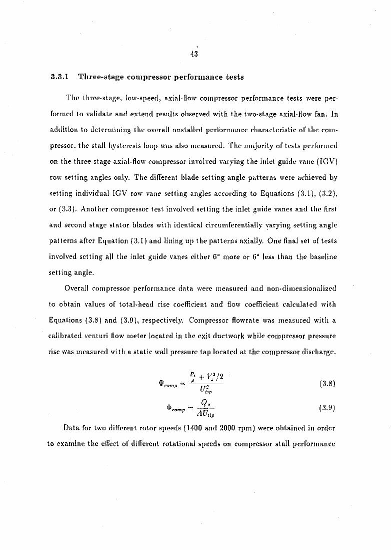
3.3.1 Three-stage compressor performance tests

The three-stage, low-speed, axial-flow compressor performance tests were per

formed to validate and extend results observed with the two-stage axial-flow fan. In

addition to determining the overall unstailed performance characteristic of the com

pressor, the stall hysteresis loop was also measured. The majority of tests performed

on the three-stage axial-flow compressor involved varying the inlet guide vane (IGV)

row setting angles only. The different blade setting angle patterns were achieved by

setting individual IGV row vane setting angles according to Equations (3.1), (3.2),

or (3.3). .Another compressor test involved setting the inlet guide vanes and the first

and second stage stator blades with identical circumferentially varying setting angle

patterns after Equation (3.1) and lining up the patterns axially. One final set of tests

involved setting all the inlet guide vanes either 6° more or 6° less than the baseline

setting angle.

Overall compressor performance data were measured and non-dimensionalized

to obtain values of total-head rise coefficient and flow coefficient calculated with

Equations (3.8) and (3.9), respectively. Compressor Howrate was measured with a

calibrated venturi flow meter located in the exit ductwork while compressor pressure

rise was measured with a static wall pressure tap located at the compressor discharge.

^ 12 = -STT— (3.8)

^ t i p

*c.,np = (3.9)

Data for two different rotor speeds (1400 and 2000 rpm) were obtained in order

to examine the effect of different rotational speeds on compressor stall performance

44

and hysteresis.

The stall point for the three-stage compressor was detected by listening for an

unmistakable and distinct audible change in sound produced by the stalling compres

sor. This audible detection of stall was accompanied by a sudden drop in flowrate

and head rise. Considerable care was taken in measuring the stall point. Experiments

near the stall point involved slowly moving the throttle to a more closed position to

reduce the overall flowrate while keeping the rotational speed constant. Fractional

adjustments in the throttle position made possible an approach to the stall point

in very small increments. Measurements were taken with each change in throttle

position. The measurements of overall performance taken just before the audible de

tection of stall occurred were considered to be for the stall point operating condition.

During any test, the stall point was approached and detected a minimum of 5 or 6

times. These tests were repeated on subsequent days to verify the repeatability of

the results. Because stall point data were consistent throughout a data run and did

not vary significantly from run to run or from day to day, it was felt that the error

band for these measurements was within the symbol used.

For the three-stage compressor, the stall recovery point was detected by opening

the throttle and thus increasing the flowrate. Again, fractional adjustments of the

throttle to more open positions were used to approach the stall recovery point in small

increments. The measurements taken just before the compressor recovered from stall

were considered to be for the stall recovery point operating condition.

45

3.3.2 Three-stage compressor results

The three-stage axial-flow compressor was tested with a variety of circumferential

variations of stationary row blade setting angles and the results are presented in this

section. One set of tests involving circumferential variations of stationary blades in

all stages was conducted. A final set of performance tests involved setting all the

inlet guide vanes either 6° more or 6° less than the baseline setting angle. Stationary

row blade setting angles were varied according to Equations (3.1), (3.2) and (3.3),

which represent the sinusoidal, rectified sine wave, and asymmetric blade setting

angle variations, respectively. The selection of appropriate setting angle patterns was

guided by results from tests performed with the two-stage axial-flow fan as well as

by observations made as tests involving the diff'erent modifications to the three-stage

compressor were completed. Stall hysteresis loops were ascertained and compared to

baseline data. The four important stall hysteresis loop operating points correspond

to the operating points of the compressor just before stall, just after stall, just before

coming out of stall, and just after coming out of stall.

The first set of results discussed corresponds to tests performed with the setting

angles of inlet guide vane row blades varying circumferentially in a pattern estab

lished by Equation (3.1). For these tests, the amplitude of setting angle variation.

Ad, remained essentially constant and the reduced frequency at stall, K,taii, was

systematically altered by changing the number of setting angle variation cycles per

rotor revolution, n. Two different rotor speeds, 1400 and 2000 rpm, were used.

The number of setting angle variation cycles per rotor revolution, n, took on

values of 1 cycle/rev, 2 cycles/rev, 3 cycles/rev, and 4 cycles/rev, which resulted in

values of reduced frequency at stall, K,taih of 0.09, 0.19, 0.28, and 0.37, respectively.

46

Of these four schedules, the best results were seen with the 2 cycles/rev pattern,

A'jiai; = 0.19. In Figure .3.8 is shown a comparison between baseline and modified

compressor performance data for the 2 cycles/rev pattern. For K,taU = 0.09, the stall

performance was worse than for the baseline configuration. For Kataii = 0.28, only

a slight improvement, not as much as for Kataii = 0.19, was observed. For K,tati =

0.37, less improvement that for Kataii — 0.28 was noted. Results of tests performed

at a higher rotational speed (2000 rpm) show nearly identical results as for the lower

rotational speed ( 1100 rpm). .Again, the stall point and recovery improvements were

most noticeable in the 2 cycles/rev scheduling of inlet guide vane row blade setting

angles.

The next set of experiments performed with the three-stage, axial-flow compres

sor involved rectified sine wave variations of inlet guide vane setting angles established

by Equation (3.2). The blade setting angle variations were periodic half sine waves

set in either a positive (larger than baseline setting angles) or negative (smaller than

baseline angles) mode which resulted respectively in either an overall decreased or

increased loading of the downstream rotor blades. Different frequencies of increased

or decreased loading were obtained by selecting an appropriate number of periodic

half-sine wave variations per rotor revolution. The amplitude of the periodic half-sine

wave variations was held constant at 6°.

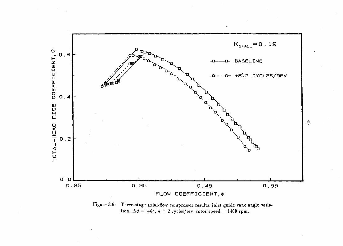
When the inlet guide vanes were set with positive half-sine wave variations, a

significant unloading of the compressor from baseline resulted for two different half-

sine wave frequencies, namely, 2 cycles per rotor revolution and 4 cycles per rotor

revolution. The stall hysteresis loop involved an unusual "kink" in recovery from

stall as shown in Figure 3.9. When the inlet guide vanes were set with negative half-

K

- 0 . 6 H Z liJ H u H IL U. ID • _ U 0 . 4

liJ in H Œ

• < lu I

I _1 < H • h-

0 . 2

STALL = 0 . 1 9

-D- D- BASELINE

..O o- ±6°, 2 CYCLES/REV

0 . 0 0 . 25 0 . 35 0 . 45

FLOW COEFFICIENT, $

0 . 55

Figure 3.8: Three-stage axial-flow compressor results, inlet guide vane angle variation, A4> = 6°, n = 2 cycles/rev, rotor speed — 1400 rpm.

48

sine wave variations, slightly more head rise but no significant change in stall point

from baseline performance were noted. Also, the negative half-sine wave variations

resulted in more hysteresis compared to baseline, see Figure 3.10.

A third set of tests performed with the three-stage axial-flow compressor in

volved the inlet guide vanes set in asymmetric blade setting angle variation patterns

according to Equation (3.3). The purpose of these variations was to achieve a higher

overall loading of the downstream rotor blades and some delay of stall onset.

Using asymmetric variations, two different tests were performed in which the

number of setting angle variation cycles per rotor revolution, n, remained constant

at 2. and the amplitudes of setting angle variation, A4>i and A<162, were altered.

In Figure 3.11 are shown results of a comparison between baseline and modified

compressor performance for which Aoi = 16° smaller than baseline (rotor loading)

and ^02 = 8° larger than baseline (rotor unloading). These data suggest that this

asymmetric variation resulted in an improvement in the stall point and also a higher

head rise compared to baseline. Results from the second asymmetric variation in

inlet guide vane setting angle with n = 2, Aéi = 20° smaller than baseline, and Act>2

= 10° larger than baseline indicated a higher head rise but degradation rather than

improvement in the stall point. For both asymmetric variations of IGV blade setting

angle, any improvement in stall recovery was uncertain.

.Additional performance tests were conducted with the inlet guide vanes, and the

first and second stage stator blades set in sinusoidal setting angle variation patterns

according to Equation (3.1). For these tests, n = 3 = 0.28) and = 6°. This

modified compressor (see Figure 3.12) produced less head rise and stalled earlier than

the baseline compressor. In contrast, the compressor build involving only inlet guide

K STALL = 0 . 1 9

' 0 . 6 H Z UJ H u M IL L. UJ o u 0 . 4

lU Ul H DC

• < Hi

Î 0.2 _1 < H O I-

-O O- BASELINE

"0----0- +6°,2 CYCLES/REV

0 . 0 0 . 25 0 . 35 0 . 45

FLOW COEFFICIENT,$

0 .55

Figure 3.9: Three-stage axial-flow compressor results, inlet guide vane angle variation, Aé = +6°, n — 2 cycles/rev, rotor speed = 1400 rpm.

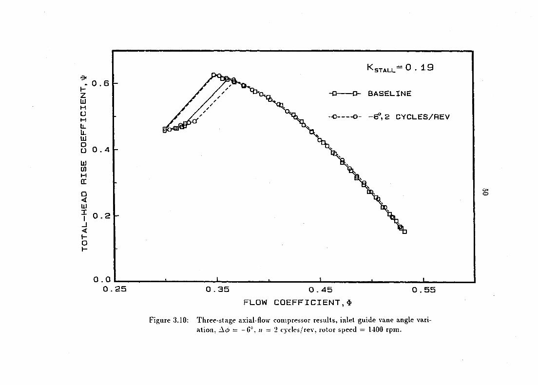
K STALL = 0 . 19

. 0 , h-z UJ H u H IL iL lU

S 0 UJ œ H DC

o < UJ

T 0 J < H O H

-O D- BASELINE

"O O- -Ef'.S CYCLES/REV

0» o

0 . 0 0 . 25 0 . 3 5 0 . 4 5

FLOW COEFFICIENT,$

0 .55

Figure 3.10; Three-stage axial-flow compressor results, inlet guide vane angle variation, Ao = -6°, II = 2 cycles/rev, rotor speed = 1400 rpm.

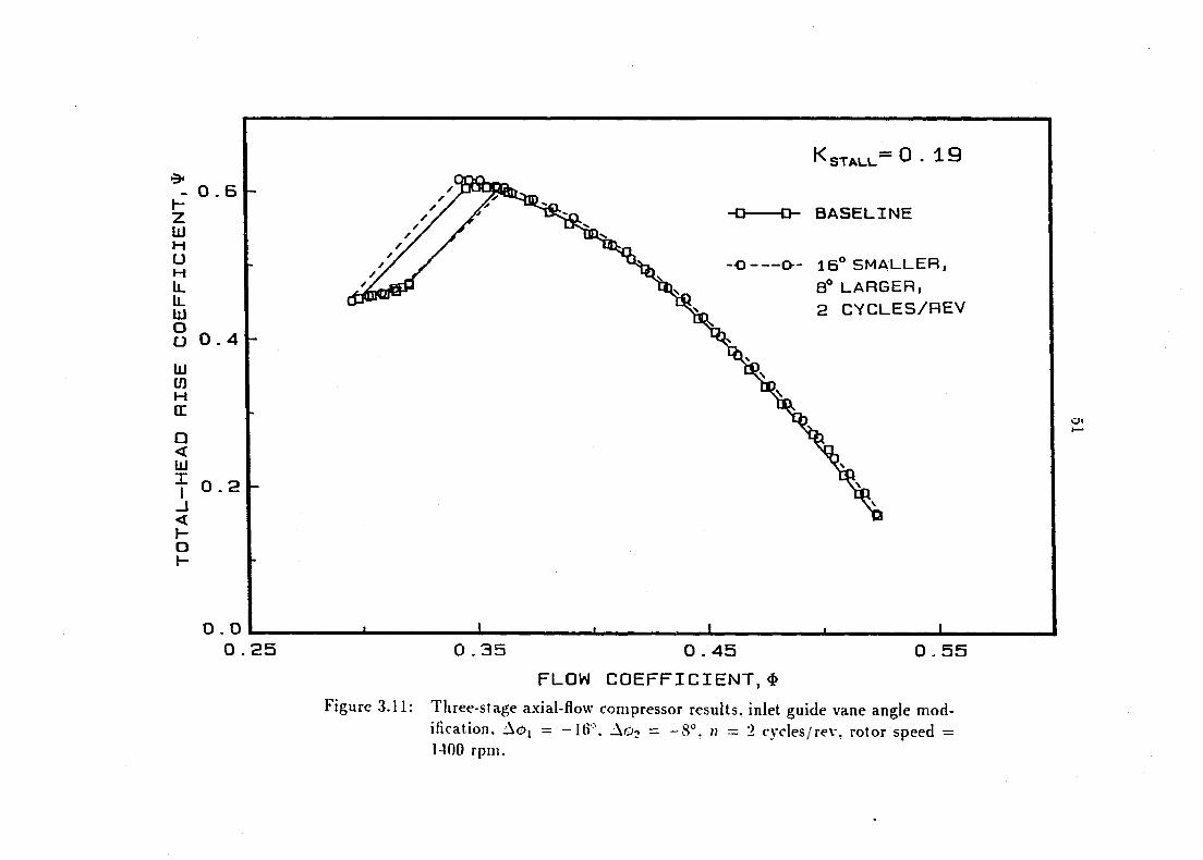
- 0 . 6 h-Z lU H U H iL IL UJ O U 0 . 4

IXJ W H IT

0 < U 1

I _l < h-O I-

0 . 2

0 . 0 0 .25

K STALL = 0.19

O- BASELINE

O- 16° SMALLER,

B® LARGER,

2 CYCLES/REV

± 0 .35 0 - 55 0 . 45

FLOW COEFFICIENT,$

Figure 3.11: Three-stage axial-flow compressor results, inlet guide vane angle modification, Ao; = -I6'\ A02 = —8°, n — '1 cycles/rev, rotor speed = 1400 rpiii.

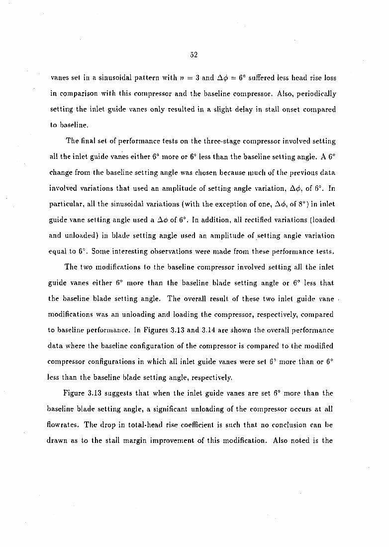
52

vanes set in a sinusoidal pattern with n = 3 and A4> = 6° suffered less head rise loss

in comparison with this compressor and the baseline compressor. Also, periodically

setting the inlet guide vanes only resulted in a slight delay in stall onset compared

to baseline.

The final set of performance tests on the three-stage compressor involved setting

all the inlet guide vanes either 6° more or 6° less than the baseline setting angle. A 6°

change from the baseline setting angle was chosen because much of the previous data

involved variations that used an amplitude of setting angle variation, Acp, of 6°. In

particular, all the sinusoidal variations (with the exception of one, A<i), of 8°) in inlet

guide vane setting angle used a of 6°. In addition, all rectified variations (loaded

and unloaded) in blade setting angle used an amplitude of setting angle variation

equal to 6°. Some interesting observations were made from these performance tests.

The two modifications to the baseline compressor involved setting all the inlet

guide vanes either 6° more than the baseline blade setting angle or 6° less that

the baseline blade setting angle. The overall result of these two inlet guide vane

modifications was an unloading and loading the compressor, respectively, compared

to baseline performance. In Figures .3.13 and 3.14 are shown the overall performance

data where the baseline configuration of the compressor is compared to the modified

compressor configurations in which all inlet guide vanes were set 6" more than or 6°

less than the baseline blade setting angle, respectively.

Figure 3.13 suggests that when the inlet guide vanes are set 6° more than the

baseline blade setting angle, a significant unloading of the compressor occurs at all

fiowrates. The drop in total-head rise coefficient is such that no conclusion can be

drawn as to the stall margin improvement of this modification. Also noted is the

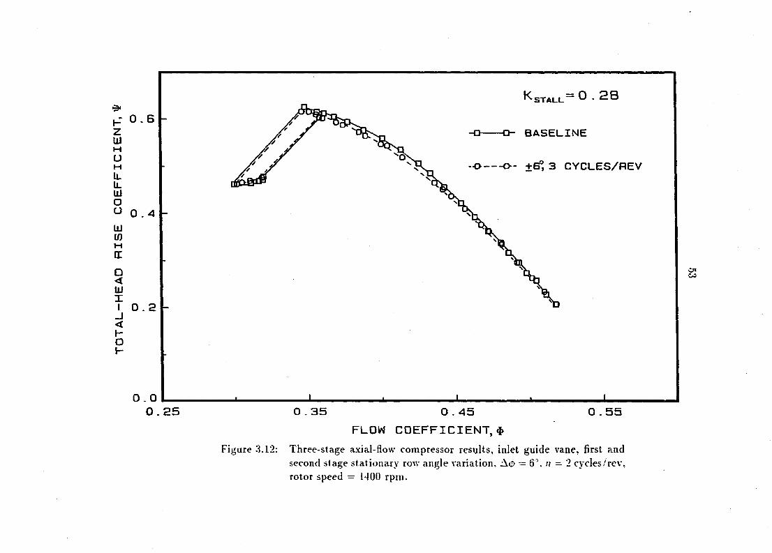
O . B Z UJ H u H IL U. lU o " 0 . 4 UJ U) M Œ

0 < tu 1

I 0 . 2 _J < H O H

^STALL O . 2B

-O D- BASELINE

-O O- +6P, 3 CYCLES/REV

O» CO

0 . 0 0 .25

X 0 - 3 5 0 . 4 5 0 . 5 5

FLOW COEFFICIENT, $

Figure 3.12: Three-stage axial-flow compressor results, inlet guide vane, first and second stage stationary row angle variation, Aô — 6". n = 2 cycles/rev, rotor speed = 1400 rpm.

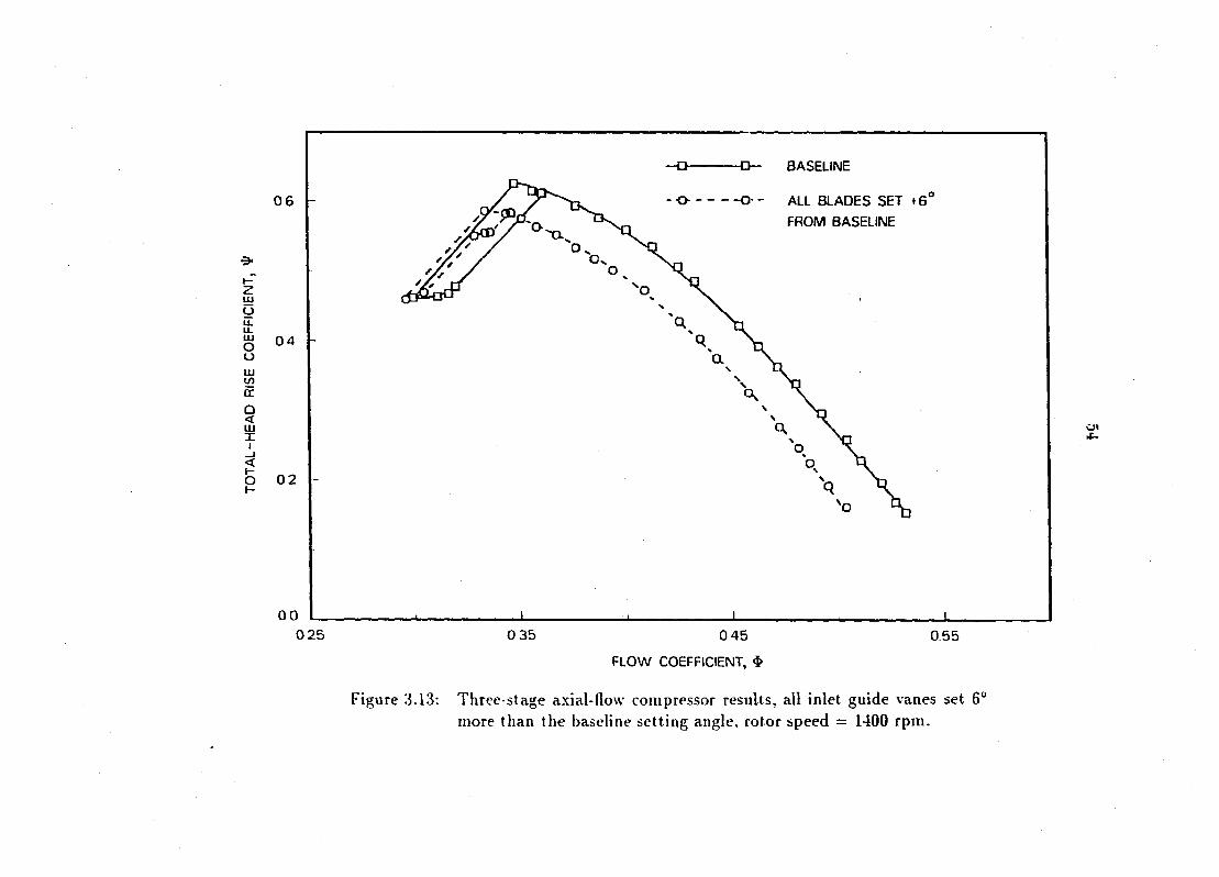
—o- -O- BASELINE

06

0 4

02

O o - ALL BLADES SET *6

FROM BASELINE

00

0 25 0 35 0 4 5

FLOW COEFFICIENT, $

0 5 5

Figure 3.13; Three-stage axial-How compressor results, all inlet guide vanes set 6° more than the baseline setting angle, rotor speed = 1400 rpni.

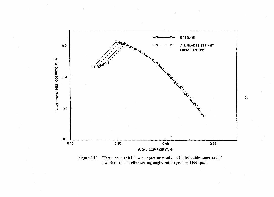
-D- 43— BASELINE

0 6

t-Z w u

ai O u (/)

Û < lU X 1

o h-

0 4

0 2

- O" "" --0-- ALL BLADES SET -6'

FROM BASELINE

Oi Cn

00

0 2 5 0 3 5 0 4 5

FLOW COEFFICIENT, *

0 5 5

Figure 3.14: Three-stage axial-flow compressor results, all inlet guide vanes set 6° less than the baseline setting angle, rotor speed — 1400 rpm.

56

strange stall hysteresis behavior. The modified compressor performance suggests

that two stall recovery points exist for this configuration. When unthrottled, the

compressor recovers quickly but not entirely. Further unthrottling is necessary to

completely recover the compressor from the stalled condition. This unusual behavior

suggests that one part of the modified compressor may be operating in a stalled

condition while another part operates unstalled. The similarity of Figure 3.9 and

Figure .3.1.3 is unmistakable. Figure 3.9 involved a rectified variation of inlet guide

vane setting angle with a +6° amplitude of setting angle in a 2/rev manner. The

unloading of the compressor from baseline behavior is evident but is slightly less than

the compressor configuration which reset all blades 6° more than baseline. Again,

the unusual hysteresis behavior is noted for this configuration as well.

Figure 3.14 reflects those results in which all inlet guide vanes were set 6° less

than the baseline blade setting angle. This figure suggests that a slight loading of

the compressor is accomplished at higher flowrates, but diminishes at lower flowrates.

The stall point for this modification occurs at a higher flow rate indicating a signifi

cant stall margin degradation from baseline. The stall hysteresis behavior no longer

exhibits the unusual two part recovery, but is simply shifted to the higher flowrates.

If these performance data are compared with those of Figure 3.10, which involved a

rectified variation of inlet guide vane setting angle with a -6° amplitude of setting

angle in a 2/rev manner, some interesting observations can be made. Figure 3.10

indicates that no penalty in stall margin occurs with the rectified variation, whereas

Figure 3.14 indicates that a significant stall margin penalty occurs when all blades

are set 6° less than baseline. This observation suggests that there is a benefit in the

unsteady loading of the compressor compared to what happens with a static loading

57

of the compressor.

3.4 Detailed Flow Measurements for Three-Stage Compressor

For the purpose of identifying some of the detailed flow characteristics caused by

the blade setting angle variations, the acquisition of detailed flow measurements (ve

locity angle and magnitude) behind the inlet guide vanes was accomplished with the

low-speed, three-stage compressor. These measurements, however, were not possible

on the Pratt fe Whitney intermediate-speed, three-stage compressor. The low-speed

compressor measurements confirmed that the absolute flow angle changed as a result

of the blade setting angle variation in the inlet guide vane row. In this case, detailed

measurements were performed for the most productive inlet guide vane setting angle

patterns (in terms of stall margin improvement) and were acquired over a portion of

the flow path cross-section area at various flow rates.

The detailed measurements were taken with a United Sensor total-pressure co

bra probe. The cobra probe was positioned in an L. C. Smith probe actuator and

was mounted on the compressor outer casing. The cobra probe head was located

downstream of the inlet guide vane exit in the measurement plane shown in Figure

.3.15. Absolute flow angle measurements were accomplished by positioning the angle

of the cobra probe such that the two side pressures were identical as indicated by a U-

tube manometer. These absolute flow angle measurements were limited to freest ream

flow regions because erroneous results occur when measuring in total-pressure (ve

locity) gradient regions. Different circumferential measurements were accomplished

by movement of the inlet guide vanes in a independent ring assembly relative to

the cobra probe position. Ten different circumferential measurement locations were

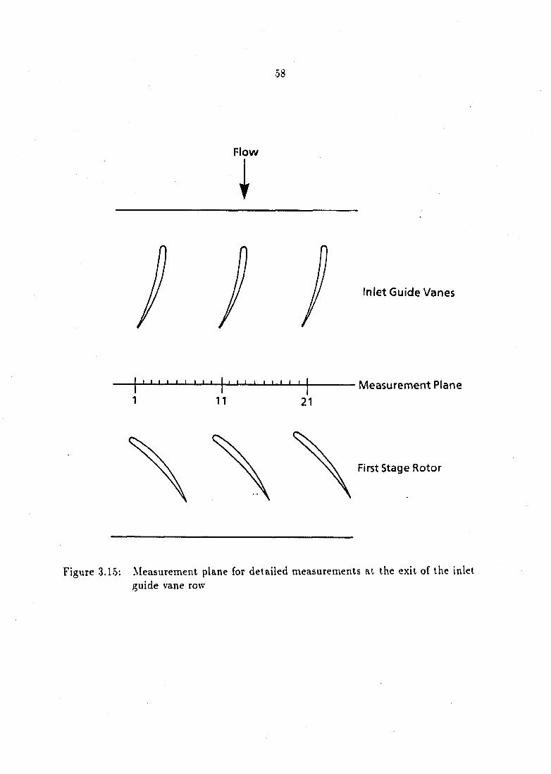
58

Flow

Inlet Guide Vanes

I I I I I I I I I I I I I I I I I I

n Measurement Plane

21

First Stage Rotor

Figure 3.15; Measurement plane for detailed measurements at the exit of the inlet guide vane row

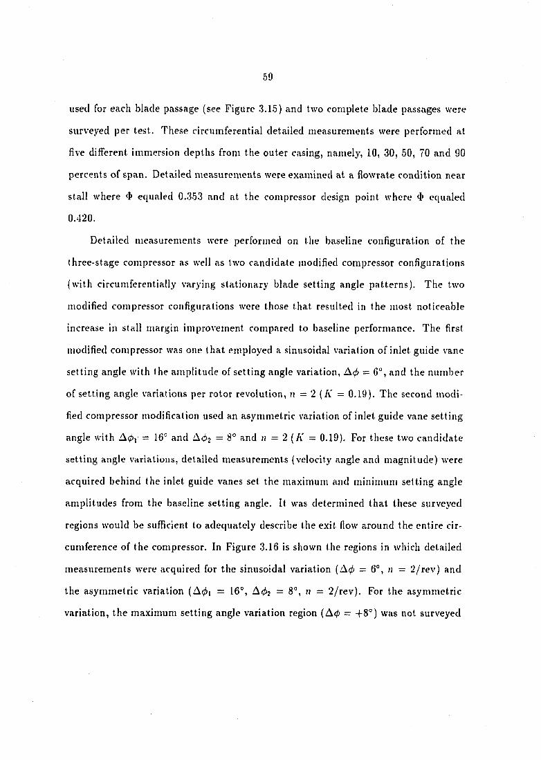
59

used for each blade passage (see Figure 3.15) and two complete blade passages were

surveyed per test. These circumferential detailed measurements were performed at

five different immersion depths from the outer casing, namely, 10, 30, 50, 70 and 90

percents of span. Detailed measurements were examined at a Howrate condition near

stall where equaled 0.353 and at the compressor design point where <5 equaled

0.420.

Detailed measurements were performed on the baseline configuration of the

three-stage compressor as well as two candidate modified compressor configurations

(with circumferentially varying stationary blade setting angle patterns). The two

modified compressor configurations were those that resulted in the most noticeable

increase in stall margin improvement compared to baseline performance. The first

modified compressor was one that employed a sinusoidal variation of inlet guide vane

setting angle with the amplitude of setting angle variation, Aç!> = 6°, and the number

of setting angle variations per rotor revolution, n = 2 {K = 0.19). The second modi

fied compressor modification used an asymmetric variation of inlet guide vane setting

angle with Aç), = 16° and ûôo = 8° and « = 2 {K = 0.19). For these two candidate

setting angle variations, detailed measurements (velocity angle and magnitude) were

acquired behind the inlet guide vanes set the maximum and minimum setting angle

amplitudes from the baseline setting angle. It was determined that these surveyed

regions would be sufficient to adequately describe the exit flow around the entire cir

cumference of the compressor. In Figure 3.16 is shown the regions in which detailed

measurements were acquired for the sinusoidal variation {Acf) = 6°, ti = 2/rev) and

the asymmetric variation (A(^i = 16°, A<^2 = 8°, u = 2/rev). For the asymmetric

variation, the maximum setting angle variation region {Aip = +8°) was not surveyed

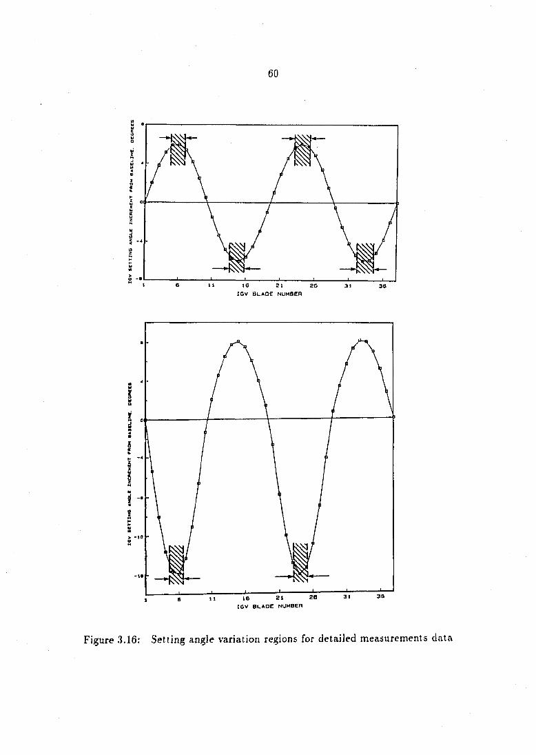
60

2CV 8LA0E NUMBER

ICV BLADE NUMBER

Figure 3,16; Setting angle variation regions for detailed measurements data

61

due to the proximity of the results with the sinusoidal variation where = +6° was

surveyed.

In Figure 3.17 is shown a typical total-pressure measurement survey for the

baseline compressor configuration at the design point and near stall operating point

covering two complete blade passages. The dashed lines separate the freestream flow

regions and wake regions where absolute flow angle measurements were possible and

not possible, respectively. The total-pressure (velocity) gradient flow regions are due

to wakes being shed from the inlet guide vanes upstream. The cobra probe side

pressure ports could not be equalized in these regions and therefore, absolute flow

angle measurements were not possible.

In Tables 3.2 and 3.3 are shown the absolute flow angle measurements for the

baseline compressor configuration at the near stall point = 0.353) and the design

operating point (<î> = 0.420) for immersion depths of 10, 30, .50, 70 and 90 percent

of span. The data presented are the average absolute flow angles for the two blade

passages surveyed. The data of Tables 3.2 and 3.3 suggest that the absolute flow angle

ranges from about 16° to 30° for both near stall point data and design operating point

data and not only varies from hub to tip but circumferentially as well. The tabular

data also suggest that the inlet guide vane performance (absolute flow angle values)

at the design point is nearly identical to the performance near stall. This notion is

consistent with the idea that inlet guide vane behavior, especially turning angle, is

independent of flowrate variations at low inlet Mach numbers (less than 0.3).

In Tables 3.4 through 3.7 some of the actual angle differences from the baseline

flow angles measured are presented for two blade setting angle variations. Additional

detailed flow measurement data are tabulated in Appendix A. Those regions surveyed

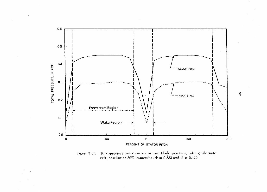
o CN X

5 V) en g a.

0 6

0 5

0.4

0 3

0.2

0 1

0 0

DESIGN POINT

NEAR STALL

Freestream Region

Wake Region

Oi to

100

PERCENT OF STATOR PITCH

200

Figure 3.17: Total-pressure variation across two blade passages, inlet guide vane exit, baseline at 50% immersion, $ = 0.353 and $ = 0.420

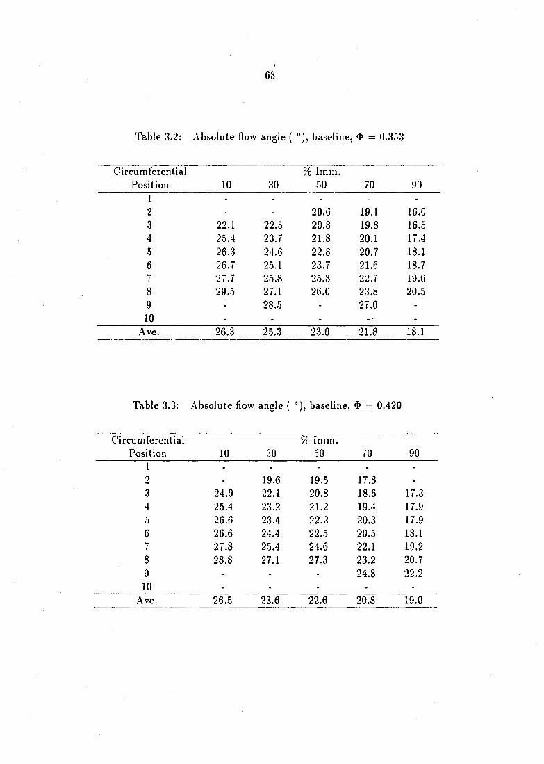
63

Table .'3.2: Absolute flow angle ( °), baseline, $ = 0.3.53

Circumferential % Imm. Position 10 30 50 70 90

1 2

- -

20.6 19.1 16.0 3 22.1 22.5 20.8 19.8 16.5 4 25.4 23.7 21.8 20.1 17.4 5 26.3 24.6 22.8 20.7 18.1 6 26.7 25.1 23.7 21.6 18.7 7 27.7 25.8 25.3 22.7 19.6 8 29.5 27.1 26.0 23.8 20.5 9 - 28.5 - 27.0 -

10 - - - - • -

Ave. 26.3 25.3 23.0 21.8 18.1

Table 3.3: Absolute flow angle ( "), baseline, 'D = 0.420


1 2

-

19.6 19.5 17.8 3 24.0 22.1 20.8 18.6 17.3 4 25.4 23.2 21.2 19.4 17.9 5 26.6 23.4 22.2 20.3 17.9 6 26.6 24.4 22.5 20.5 18.1 7 27.8 25.4 24.6 22.1 19.2 8 28.8 27.1 27.3 2&2 20.7 9 - - - 24.8 22.2

10 - - - - -

Ave. 26.5 23.6 22.6 20.8 19.0

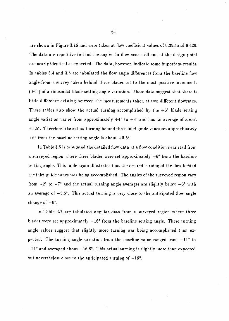
64

are shown in Figure 3.16 and were taken at flow coefficient values of 0.353 and 0.420.

The data are repetitive in that the angles for flow near stall and at the design point

are nearly identical as expected. The data, however, indicate some important results.

In tables 3.4 and 3.5 are tabulated the flow angle differences from the baseline flow

angle from a survey taken behind three blades set to the most positive increments

(+6°) of a sinusoidal blade setting angle variation. These data suggest that there is

little difference existing between the measurements taken at two different flowrates.

These tables also show the actual turning accomplished by the -r6° blade setting

angle variation varies from approximately +4° to +8° and has an average of about

-f5.5°. Therefore, the actual turning behind three inlet guide vanes set approximately

4-6° from the baseline setting angle is about 4-5.5°.

In Table 3.6 is tabulated the detailed flow data at a flow condition near stall from

a surveyed region where three blades were set approximately —6° from the baseline

setting angle. This table again illustrates that the desired turning of the flow behind

the inlet guide vanes was being accomplished. The angles of the surveyed region vary

from -2° to -7° and the actual turning angle averages are slightly below —6° with

an average of —5.6°. This actual turning is very close to the anticipated flow angle

change of -6°.

In Table 3.7 are tabulated angular data from a surveyed region where three

blades were set approximately -16° from the baseline setting angle. These turning

angle values suggest that slightly more turning was being accomplished than ex

pected. The turning angle variation from the baseline value ranged from -11° to

—21° and averaged about -16,8°. This actual turning is slightly more than expected

but nevertheless close to the anticipated turning of —16°.

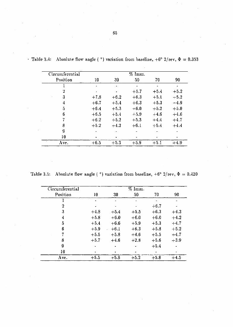
65

• Table 3.4: Absolute flow angle ( °) variation from baseline, +6° 2/rev, $ = 0.353


1 2 - - +5.7 +5.4 +5.2 3 +7.8 +6.2 +6.3 +5.1 +5.2 4 +6.7 +5.4 +6.3 +5.3 +4.9 5 +6.4 +5.3 +6.0 +5.2 +5.0 6 +6.5 +5.4 +5.9 +4.6 +4.6 7 +6.2 +5.2 +5.3 +4.4 +4.7 8 +5.2 +4.2 +6.1 +5.4 +4.4 9 . . . . . 10 -

Ave. +6.0 +5.3 +0.9 +5.1 +4.9

Table 3.5; .Absolute flow angle ( °) variation from baseline, +6° 2/rev, $ = 0.420


1 2

- - -

+6.7 -

3 +4.8 +5.4 +5.5 +6.3 +4.3 4 +5.8 + 6.0 +6.0 +6.0 +4.2 5 +5.4 +6.6 +5.9 +5.3 +4.7 6 +5.9 +6.1 +6.3 +5.8 +5.2 7 +5.5 +5.8 +4.6 +5.5 +4.7 8 +5.7 +4.6 +2.8 +5.6 +3.9 9 - - - +5.4 -

10 - - - - -

Ave. +5.5 +5.8 +5.2 +5.8 +4.5

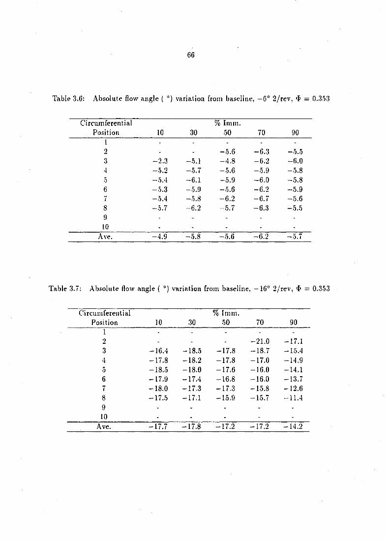
66

Table 3.6: .Absolute flow angle ( °) variation from baseline, —6° 2/rev, «P = 0.353

Circumferential % I mm. Position 10 30 50 70 90

1 - - - - -

2 - - -5.6 -6.3 -5.5 3 -2.3 -5.1 -4.8 -6.2 -6.0 4 -5.2 -5.7 —0.6 —5.9 -5.8 5 -5.4 -6.1 -5.9 -6.0 -5.8 6 -5.3 -5.9 -5.6 -6.2 -5.9 7 -5.4 -5.8 -6.2 -6.7 -5.6 8 —5.7 -6.2 -5.7 -6.3 -5.5 9 - - - - -

10 - - - - -

.Ave. -4.9 -5.8 -5.6 -6.2 -5.7

Table 3.7: .Absolute flow angle ( °) variation from baseline, —16° 2/rev, = 0.353


I 2 - - - -21.0 -17.1 3 -16.4 -18.5 -17.8 -18.7 -15.4 4 -17.8 -18.2 -17.8 -17.0 -14.9 5 -18.5 -18.0 -17.6 -16.0 -14.1 6 -17.9 -17.4 -16.8 -16.0 -13.7 7 -18.0 -17.3 -17.3 -15.8 -12.6 8 -17.5 -17.1 -15.9 -15.7 -11.4 9

Ave. -17.7 -17.8 -17.2 -17.2 -14.2

67

3.4.1 Velocity diagram calculations using detailed measurements

In Chapter 5 of this dissertation, estimates for the reduced frequency and rotor

inlet flow angle variation are made using a simplified approach outlined in reference

[12]. These estimates were made for midspan geometry only at the stall condition.

The radial survey of detailed measurements discussed in the previous section can be

used to produce a more precise calculation of the actual reduced frequency at stall,

and the maximum and minimum rotor inlet flow angle variations. The analysis

involves using hub to tip detailed measurements for the baseline flow angle to solve for

the baseline velocity triangles at the stall point and/or design point. These baseline

velocity triangles are then compared to those in which detailed measurements were

taken behind those few inlet guide vanes reset to the minimum and maximum setting

angle amplitudes from baseline.

In order to construct blade velocity diagrams from detailed measurements, the

radial static pressure distribution at the exit to the inlet guide vanes must be calcu

lated. This is accomplished by solving the hydrodynamic equation of equilibrium for

the flow exiting the inlet guide vanes. .Assuming radial velocities are equal to zero,

the hydrodynamic equation of equilibrium can be written,

I d P _ IV

p dr r (.3.10)

or

(3.11) dr

From blade velocity triangle relations,

VE — V sin/? (3.12)

68

Substitution of Equation (3.12) into Equation (3.11) results in,

dP pV^ s in ' l3

dr r

And using Bernoulli's equation for incompressible flow,

P V P,

p ' 2 ~ p

or

(3.13)

(3.14)

Substituting this result into Equation (3.13) gives the final form of the hydrodynamic

equation of equilibrium which is written as

aP ^ 2sin',d(P,-P) or r

Equation (3.16) indicates that a knowledge of the total-pressure, P,, and the

absolute flow angle, 3, at different radial locations, r, may be used to solve the static

pressure distribution. The average values of the absolute flow angle and total-pressure

circumferential survey at difl'erent radial locations given in the previous section and

in Appendix A were used in the analysis. Equation (3.16) was solved on a computer

using a curve-fitting algorithm along with an initial estimate for the static pressure

distribution. Because detailed measurements were acquired at five different radii,

namely 10, 30, .50, 70 and 90 percent immersion depths, a five point curve-fitting

algorithm was used. The initial estimate for the static pressure distribution involved

using the measured value of static wall pressure and a straight line variation of static

pressure from hub to tip. The algorithm then adjusted the individual static pressure

values at the five different radii in successive iterations until the left hand side of

69

Equation (3.16) equaled the right hand side for the different radial locations. With

the static distribution solution, the blade velocity diagrams were constructed with the

use of Equation (3.1.5) for the absolute velocity, V, Equation (3.12) and Equations

(5.4) through (5.9) of Chapter 5.

The process of solving for the static pressure distribution and blade velocity tri

angles was repeated for an operating condition near stall and at the design operating

point. In Table 3.8 are summarized the results of the baseline velocity diagram cal

culations. These data are the static pressure, P,,, absolute flow angle, âx, absolute

flow velocity, absolute tangential velocity, I, blade velocity, relative tangen

tial velocity, «•«,, axial velocity, Vj,, relative velocity, u'l, relative flow angle, i3[ and

the reduced frequency at stall, Kstaih for each radial location. The value of K,tati is

calculated from the following equation.

Equation (3.17) is derived by rearranging Equation (3.5), V = a',, and substituting

values for n, c and RPM, where

u — 2 cycles per rotor revolution

c = 1.20 in.

RPM = 1400 rpm

Further calculation of the minimum and maximum rotor inlet How angle variation

from the baseline value may be made by using absolute flow angle measurements for

circumferential blade setting angle variations. For this calculation, it is assumed

that the axial velocity remains constant from hub to tip regardless of the imposed

variation in inlet guide vane setting angle. Therefore, the axial velocities calculated

TO

from the baseline detailed measurement data become the axial velocities for the

modified velocity diagram calculations. By using the following equation,

and Equations (5.4) through (5.9) this is accomplished.

In Tables 3.9 through 3.11 are tabulated some of the velocity triangle calculations

for those modified compressor detailed measurements whose regions are shown in

Figure 3.16. .Additional velocity triangle calculations for the design point conditions

are tabulated in .Appendix B. Of particular importance in these tables is the rotor

inlet flow angle variation from baseline, A/3J. This quantity is a measure of rotor

loading or unloading from hub to tip. .A value of +1.0° would indicate a increase

in rotor relative flow angle of 1.0° when the rotor passes through the particular setting

angle variation. Similarly, a value of —1.0° would indicate a decrease in rotor

relative flow angle of 1.0°.

.A comparison is made between the detailed measurement calculations and the

estimated values for the reduced frequency and rotor inlet flow angle variation for the

three-stage compressor. Because estimated values of reduced frequency and extent of

rotor inlet flow angle variation exist only for midspan geometry, these values are com

pared. Table 3.8 indicates that the midspan reduced frequency at stall from detailed

measurements is 0.19. This value is identical to the estimated value for midspan

reduced frequency at stall (K,taii = 0.19). Also, midspan values for the extent of

rotor inlet flow angle variation calculated with detailed data are nearly identical to

estimated values (Table 5.4). This comparison suggests that the original estimates

for reduced frequency and extent of rotor inlet flow angle variation are accurate. This

71

conclusion is important in determining the blade setting angle variation for the Pratt

& Whitney compressor.

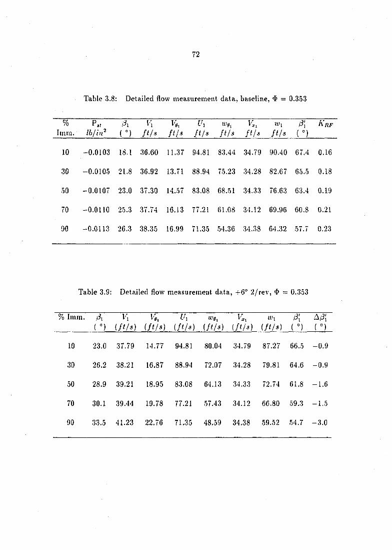
72

Table 3.8: Detailed flow measurement data, baseline, = 0.353

% Pjt i^i 11 Vfi, W9^ K, lUi f3[ A'flf Imm. Ib / iu^ ( ° ) f t / s f t / s f t / s f t / s f t / s f t / s ( ° )

10 -0.0103 18.1 36.60 11.37 94.81 83.44 .34.79 90.40 67.4 0.16

.30 -0.010.5 21.8 36.92 13.71 88.94 7.5.23 34.28 82.67 65.5 0.18

50 -0.0107 23.0 37.30 14.57 83.08 68.51 34.33 76.63 63.4 0.19

70 -0.0110 25.3 37.74 16.13 77.21 61.08 34.12 69.96 60.8 0.21

90 -0.0113 26.3 38.35 16.99 71.35 54.36 34.38 64.32 .57.7 0.23

Table 3.9: Detailed flow measurement data, +6° 2/rev, = 0.353

% Imm. Vi Vtf, Ui wg, V;, wx l3[ ( ° ) { f i / s ) ( f t / s ) ( f t j s ) ( î t / s ) i f t l s ) ( f t / s ) ( ° ) ( ° )

10 23.0 37.79 14.77 94.81 80.04 34.79 87.27 66.5 -0.9

30 26.2 .38.21 16.87 88.94 72.07 34.28 79.81 64.6 -0.9

50 28.9 39.21 18.95 83.08 64.13 34.33 72.74 61.8 -1.6

70 30.1 39.44 19.78 77.21 57.43 34.12 66.80 59.3 -1.5

90 33.5 41.23 22.76 71.35 48.59 34.38 .59.52 54.7 -3.0

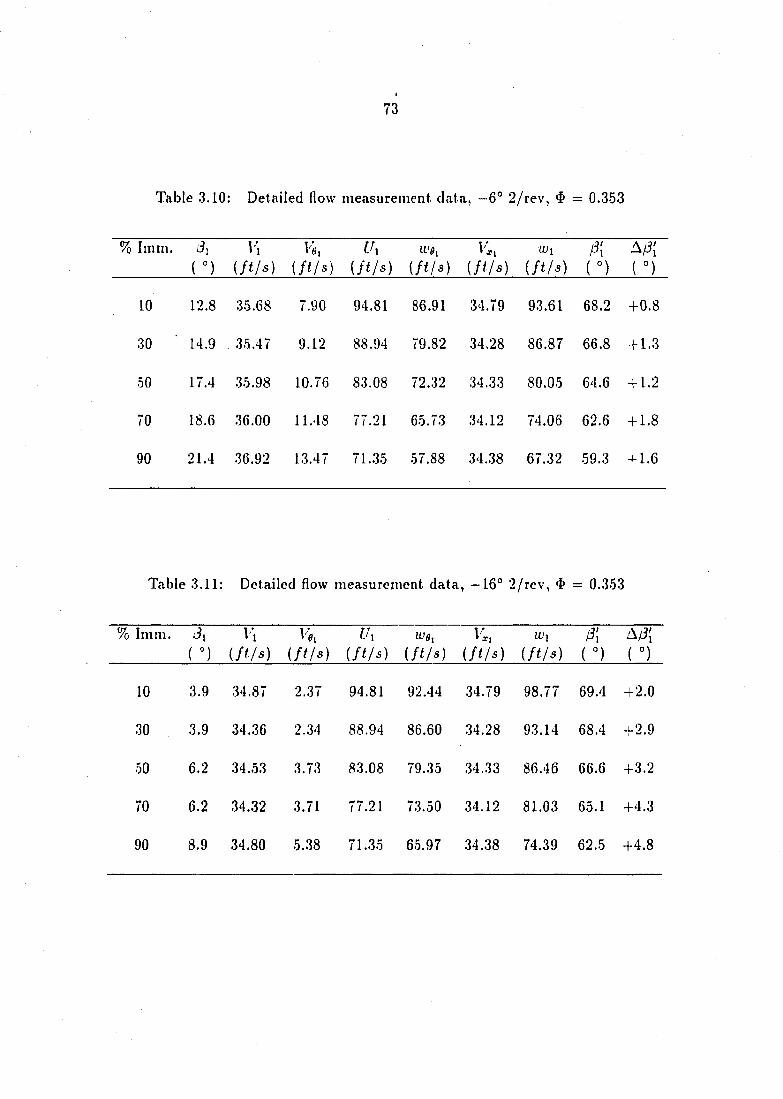
73

Table 3.10: Detailed flow measurement data, -6° 2/rev, <5 — 0.353

% I mm. ( °)

V'l ( f t / s ) (/(/a)

f A i f t / s )

U'fl, (/(/a)

t'L., (/f/a)

(wi (/f/a) i ° ) ( °)

10 12.8 .35.68 7.90 94.81 86.91 34.79 93.61 68.2 +0.8

30 14.9 . 35.47 9.12 88.94 79.82 34.28 86.87 66.8 + 1.3

50 17.4 35.98 10.76 83.08 72.32 34.33 80.05 64.6 + 1.2

70 18.6 .36.00 11.48 77.21 65.73 34.12 74.06 62.6 + 1.8

90 21.4 36.92 13.47 71..35 57.88 34.38 67.32 59.3 + 1.6

Table 3.11: Detailed flow measurement data ,-16° 2 /rev, = 0.353

% Imm.

( n

V, i f f / s )

1',. ( f t f s )

u , ( / f/j) (/f/a)

v;. (/f/a)

W i (/(/a) ( °)

Af3[ ( °)

10 3 .9 .34.87 2.37 94.81 92.44 .34.79 98.77 69.4 +2.0

30 3.9 .34.36 2.34 88.94 86.60 34.28 93.14 68.4 +2.9

50 6.2 34.53 3.73 83.08 79.35 34.33 86.46 66.6 +3.2

70 6.2 34.32 3.71 77.21 73.50 .34.12 81.03 65.1 +4.3

90 8.9 34.80 5.38 71.35 65.97 .34.38 74.39 62.5 +4.8

74

3.5 Low-Speed Compressor Conclusions

A review of literature related to dynamic stall was accomplished to get an idea of

what reduced frequency at stall and what amplitude of blade setting angle variation

should be used for tests involving a two-stage axial-flow fan and a three-stage axial-

How compressor. Preliminary tests were performed on a two-stage axial-flow fan

to investigate whether or not the stall margin of an axial-flow fan or compressor

could be improved by appropriately scheduling the setting angles of the stationary

blades upstream of a rotor. A three-stage axial-flow research compressor was tested

with a variety of inlet guide vane circumferentially varying setting angle patterns

to confirm results obtained with the two-stage fan and to reach further conclusions

about stall margin improvement capability. Additional three-stage compressor tests

were performed with inlet guide vanes and first and second stage stator blades set in

identical circumferentially varying setting angle patterns. A final set of performance

tests were performed with all the inlet guide vanes set either 6° more or 6° less than

the baseline setting angle. Some detailed measurements of the flow exiting the inlet

guide vane row of the three-stage compressor were also acquired for the baseline

compressor configuration as well as some modified compressor configurations.

The review of relevant literature suggested that the use of a reduced frequency

value in the range from 0.30 to 0.35 would give the most benefit in terms of improving

the stall margin of a compressor rotor row. The amplitude of airfoil oscillation, which

varied from 5° to 20° in the literature reviewed, gave guidance about the magnitude

of blade setting angle, A(6, used in the tests.

Tests of the two-stage axial-flow fan indicated that for several difl'erent circum

ferential variation patterns of stator blade setting angle, the fan stall limit could

75

be moved to lower flow coefficients. It was also noted that the magnitude of the

stall margin increase was a function of the reduced frequency at stall, K,taih and

the amplitude of blade setting angle, The optimum increase in stall margin was

observed to occur when the reduced frequency at stall was near a value of 0.3 and

the amplitude of blade setting angle was in the range of from 5° to 7°.

Tests of the three-stage axial-flow research compressor involving a variety of cir-

cumferentially varying IGV row blade setting angle patterns set according to Equa

tion (3.1) suggest that stall margin, head-rise production, and stall hysteresis could

be improved by the appropriate setting of the IGV row blade setting angles in a

circumferentially varying pattern. For these tests, the optimum reduced frequency at

stall for increasing the stall margin was near 0.19. In addition, a slight shift in the

"out of stall" point with compressor modification indicates that the modified com

pressor was actually relieved from stall sooner than the baseline compressor. The

amplitude of blade setting angle, Aoi, for the above modified compressor was held

constant at 6°.

Tests of the three-stage axial-flow compressor with the inlet guide vanes set

according to Equation (3.2), i.e., rectified sine wave angle variations, suggest that

one-sided variations are not useful. When the rotor blades were periodically unloaded

only, the drop in head-rise production from baseline was appreciable, too much to

justify any gain in stall margin achieved. When the rotor blades were periodically

loaded only, the increase in head-rise production was minimal and no gain in stall

margin was observed. A significant degradation in stall point recovery occurred.

Tests of the three-stage axial-flow compressor with the inlet guide vanes set ac

cording to Equation (3.3), i.e., asymmetric angle variations, suggest that asymmetric

76

angle variations can lead to increased head-rise production and improved stall margin.

However, stall recovery improvement was not observed. Also, larger angle variation

amplitudes result in significant stall margin degradation.

test of the three-stage axial-flow compressor with the inlet guide vanes, and

first and second stage stator blades all set in the same circuniferentially varying

periodic and symmetrical pattern suggest that while setting an accelerating row of

blades, e.g., inlet guide vanes, in such a pattern may improve modified compressor

performance in terms of stall margin, stall hysteresis and head-rise production, sim

ilar setting of diffusing blades, e.g., stator blades, may lead to worsened modified

compressor performance.

.A. set of tests was performed on the three-stage compressor in which all inlet

guide vanes were set either 6° more or less than the baseline setting angle. Results

suggested that a significant unloading of the compressor occurred when the blades

were set 6' more than baseline. Only a slightly higher loading was achieved when

the blades were set 6° less than baseline. These tests also indicated the benefit of

periodically varying the blade setting angles around the circumference as compared

to simply setting all the blades 6° more or less than the baseline setting angle.

Detailed measurements taken on the low-speed, three-stage compressor suggested

that the actual turning of the flow behind the inlet guide vanes was approximately

equal to the amplitude of setting angle variation in the inlet guide vane row. The

data also confirmed the idea that inlet guide vane turning is independent of varying

fiowrates at Mach numbers less than 0.3. A comparison between detailed measure

ment calculated and estimated values of reduced frequency at stall and extent of

rotor inlet flow angle variation suggest that the estimated values are valid.

I I

Results from the low-speed compressors suggested that slight improvements in

stall margin and recovery were possible with compressor modifications using an ap

propriate scheduling of the setting angles of the inlet guide vanes upstream of a rotor.

The varying success of these low-speed tests was primarily a function of the setting

angle pattern used, the reduced frequency at stall, and the estimated rotor inlet flow

angle variation. These preliminary extensions of dynamic stall notions to turboma-

chine flows suggests that further studies were warranted. For this reason, the idea for

improving the stall margin through the use of circumferentially varying stationary

blade setting angles was tested on a higher-speed, three-stage, axial-flow compressor.

78

4. PRATT & WHITNEY COMPRESSOR

A Pratt & Whitney, intermediate-speed, three-stage, axial-flow research com

pressor was used to test the effects of compressibility on the proposed method for

improving the stall margin of axial-flow compressors. The research compressor and

related equipment, located in the Turbomachinery Components Research Labora

tory of Iowa State University, are described in the following sections. The design and

installation of the data acquisition system used on the Pratt &: Whitney research

compressor is also described.

4.1 Pratt & Whitney Axial-Flow Compressor

The Pratt & Whitney, intermediate-speed, three-stage, axial-flow compressor is

described in this section. Shown in Figure 4.1 is the compressor test stand including

(from right to left) the drive motor, gearbox, inlet flow ductwork, compressor, flowrate

measurement section, throttle housing and exit flow ductwork. This compressor was

used for testing the effects of compressibility on the proposed method of improving

the stall margin of axial-flow compressors.

The configuration of the compressor consisted of a set of inlet guide vanes fol

lowed by three stages of rotor and stator blade rows (see Figure 4.2). The blade

rows were within an annulus having a constant tip (24.000 in. (0.610 m)) diameter.

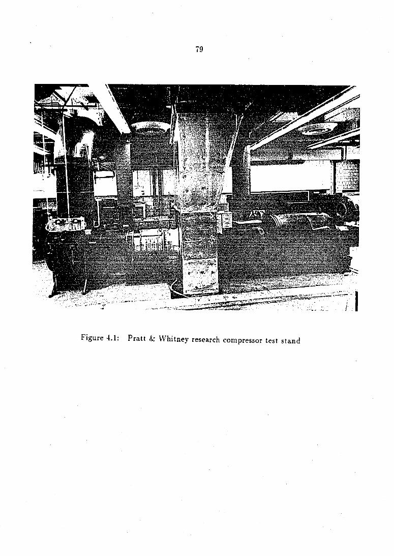
mm

Figure 4,1: Pratt & Whitney research compressor test stand

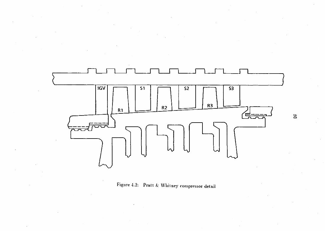
r~i

IGV

R3 R2

A/

Figure 4.2: Pratt & Whitney compressor detail

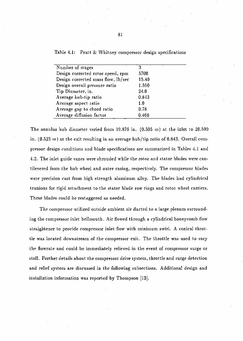
81

Table 4.1: Pratt & Whitney compressor design specifications

Number of stages Design corrected rotor speed, rpm Design corrected mass flow, lb/sec Design overall pressure ratio Tip Diameter, in. Average hub-tip ratio Average aspect ratio Average gap to chord ratio Average diffusion factor

5700 15.40 1.350 24.0 0.843 1.0 0.78

0.468

3

The annulus hub diameter varied from 19.876 in. (0.505 m) at the inlet to 20.590

in. (0.523 rn ) at the exit resulting in an average hub/tip ratio of 0.843. Overall com

pressor design conditions and blade specifications are summarized in Tables 4.1 and

4.2. The inlet guide vanes were shrouded while the rotor and stator blades were can-

tilevered from the hub wheel and outer casing, respectively. The compressor blades

were precision cast from high strength aluminum alloy. The blades had cylindrical

trunions for rigid attachment to the stator blade row rings and rotor wheel carriers.

These blades could be restaggered as needed.

The compressor utilized outside ambient air ducted to a large plenum surround

ing the compressor inlet beilrnouth. .Air flowed through a cylindrical honeycomb flow

straightener to provide compressor inlet flow with minimum swirl. A conical throt

tle was located downstream of the compressor exit. The throttle was used to vary

the flowrate and could be immediately relieved in the event of compressor surge or

stall. Further details about the compressor drive system, throttle and surge detection

and relief system are discussed in the following subsections. Additional design and

installation information was reported by Thompson [13].

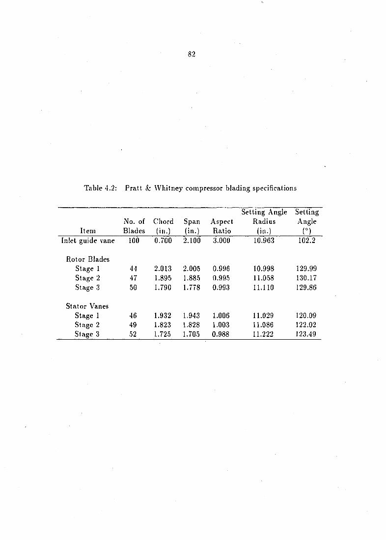
82

Table 4.2: Pratt & Whitney compressor blading specifications

Setting Angle Setting No. of Chord Span Aspect Radius Angle

Item Blades (in.) (in.) Ratio (in.) ( ° )

Inlet guide vane 100 0.700 2.100 3.000 10.963 102.2

Rotor Blades Stage 1 44 2.013 2.005 0.996 10.998 129.99 Stage 2 47 1.895 1.885 0.995 11.058 130.17 Stage 3 50 1.790 1.778 0.993 11.110 129.86

Stator Vanes Stage 1 46 1.932 1.943 1.006 11.029 120.09 Stage 2 49 1.823 1.828 1.003 11.086 122.02 Stage 3 52 1.725 1.705 0.988 11.222 123.49

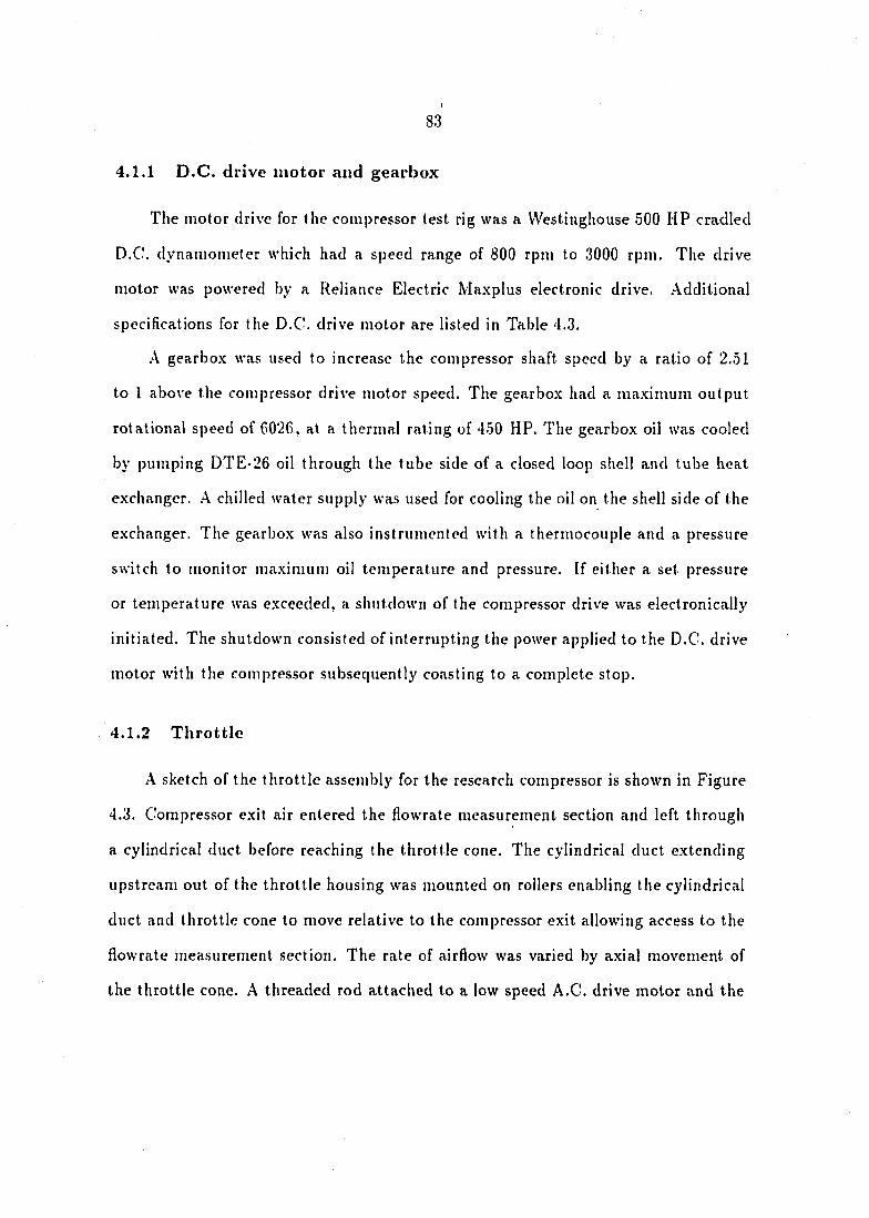
83

4.1.1 D.C. drive motor and gearbox

The motor drive for the compressor test rig was a Westinghouse 500 HP cradled

D.C. dynamometer which had a speed range of 800 rpm to 3000 rpm. The drive

motor was powered by a Reliance Electric Maxplus electronic drive. .Additional

specifications for the D.C\ drive motor are listed in Table 4.3.

A gearbox was used to increase the compressor shaft speed by a ratio of 2.51

to 1 above the compressor drive motor speed. The gearbox had a maximum output

rotational speed of 6026, at a thermal rating of 450 HP. The gearbox oil was cooled

by pumping DTE 26 oil through the tube side of a closed loop shell and tube heat

exchanger. A chilled water supply was used for cooling the oil on the shell side of the

exchanger. The gearbox was also instrumented with a thermocouple and a pressure

switch to monitor maximum oil temperature and pressure. If either a set pressure

or temperature was exceeded, a shutdown of the compressor drive was electronically

initiated. The shutdown consisted of interrupting the power applied to the D.C. drive

motor with the compressor subsequently coasting to a complete stop.

4.1.2 Throttle

A sketch of the throttle assembly for the research compressor is shown in Figure

4.3. Compressor exit air entered the flowrate measurement section and left through

a cylindrical duct before reaching the throttle cone. The cylindrical duct extending

upstream out of the throttle housing was mounted on rollers enabling the cylindrical

duct and throttle cone to move relative to the compressor exit allowing access to the

flowrate measurement section. The rate of airflow was varied by axial movement of

the throttle cone. A threaded rod attached to a low speed A.C. drive motor and the

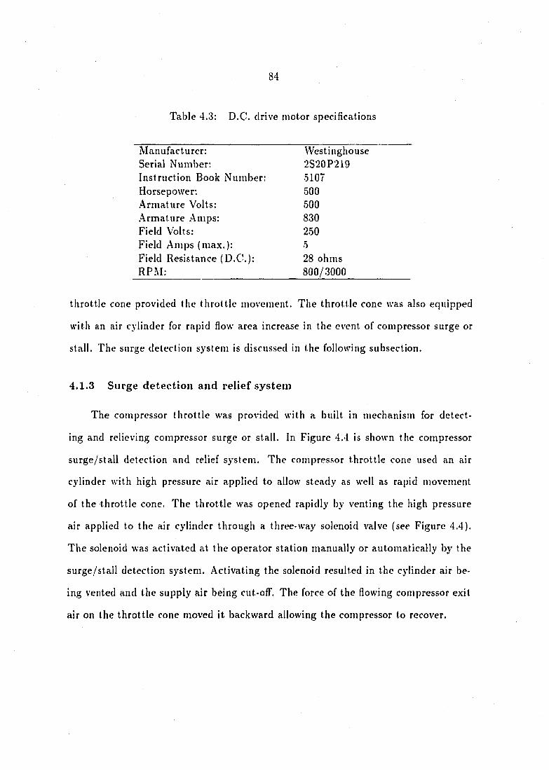
84

Table 4.3: D.C. drive motor specifications

Manufacturer: Serial Number: Instruction Book Number: Horsepower: .Armature Volts: Armature .Amps: Field Volts: Field .Amps (max.): Field Resistance (D.C.): RPM:

28 ohms 800/3000

5107 500 500 830 250 5

2S20P219 VVestinghouse

throttle cone provided the throttle movement. The throttle cone was also equipped

with an air cylinder for rapid flow area increase in the event of compressor surge or

stall. The surge detection system is discussed in the following subsection.

4.1.3 Surge detection and relief system

The compressor throttle was provided with a built in mechanism for detect

ing and relieving compressor surge or stall. In Figure 4.4 is shown the compressor

surge/stall detection and relief system. The compressor throttle cone used an air

cylinder with high pressure air applied to allow steady as well as rapid movement

of the throttle cone. The throttle was opened rapidly by venting the high pressure

air applied to the air cylinder through a three-way solenoid valve (see Figure 4.4).

The solenoid was activated at the operator station manually or automatically by the

surge/stall detection system. .Activating the solenoid resulted in the cylinder air be

ing vented and the supply air being cut-off. The force of the flowing compressor exit

air on the throttle cone moved it backward allowing the compressor to recover.

Flowrate Measurement Section

Throttle Housing

Compressor

Motor

Air

Throttle

J I "" " 1 i"

r—S /

Figure 4.3: Pratt & Whitney throttle section detail

Vent Solenoid Valve

Surge Protector 0.035 in.dia Capillary n

Release Reset

Vent c 125 psig Air Source Diff. Pressure

Transducer in. dia

Orifice

Electric Drive

Air Cylinder

Compressor Discharge Duct Throttle Ass y

Figure 4.4: Pratt & VVliitney automatic surge detection and relief system

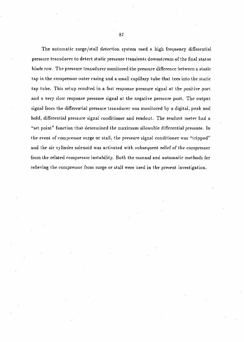
87

The automatic surge/stall detection system used a high frequency difl'erential

pressure transducer to detect static pressure transients downstream of the final stator

blade row. The pressure transducer monitored the pressure difference between a static

tap in the compressor outer casing and a small capillary tube that tees into the static

tap tube. This setup resulted in a fast response pressure signal at the positive port

and a very slow response pressure signal at the negative pressure port. The output

signal from the differential pressure transducer was monitored by a digital, peak and

hold, differential pressure signal conditioner and readout. The readout meter had a

"set point" function that determined the maximum allowable differential pressure. In

the event of compressor surge or stall, the pressure signal conditioner was "tripped"

and the air cylinder solenoid was activated with subsequent relief of the compressor

from the related compressor instability. Both the manual and automatic methods for

relieving the compressor from surge or stall were used in the present investigation.

88

4.2 Pratt & Whitney Compressor Data Acquisition System

The Pratt & Whitney compressor data acc|uisition system was designed and

implemented during the course of this investigation and is described in detail in the

following subsections. The two major areas of data acquisition, namely, pressure and

temperature scanning are discussed. The selection of appropriate data acquisition

equipment for the testing environment is described.

4.2.1 Pressure system

Most of the pressure measurements in the intermediate-speed, three-stage, axial-

flow compressor were made with the system shown in Figure 4.5. The system involved

a Scanivalve Z0C14 electronic pressure scanning module specifically designed for tur

bine engine testing applications. This state-of-the-art pressure scanner was chosen

for its compact size, high scanning rate, accuracy and flexibility when used for aero

dynamic testing. In addition, the Scanivalve Z0C14 along with support equipment

from Scanivalve could be easily incorporated into existing data acquisition equip

ment already available in the research laboratory. The methods of installation and

operation of the Scanivalve pressure system are discussed in further detail.

The Scanivalve Z0C14 is an electronic pressure scanner which accepts 32 pneu

matic pressure inputs and converts them to computer compatible electrical signals.

The Z0C14 module (see Figure 4.6) contained 32 individual silicon pressure sensors,

each with a nominal differential pressure range of 10 psi. The 10 psi differential

range was selected because it enveloped the maximum anticipated pressure levels in

the compressor and still allowed good full scale accuracy. The maximum scanning

rate of the scanner is lOOkHz when used with a photo-optical Darlington switch. Ac-

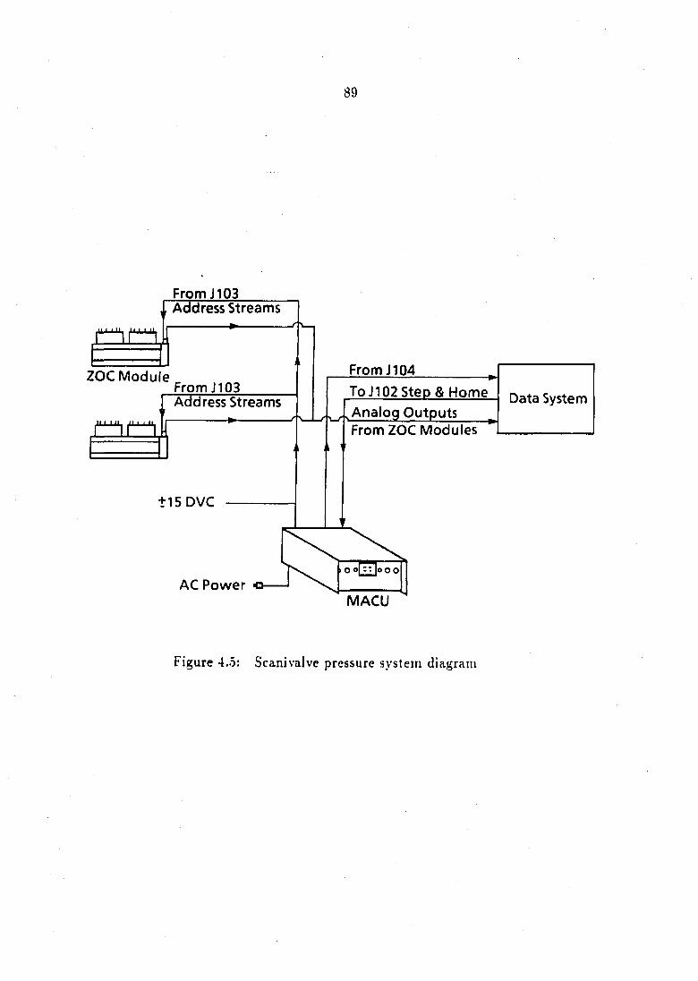
89

From J103 Address Streams

^<1 t 1 11 M I I 11

From J104 ZOC Module From J103 To J102 Step & Home

Analog Outputs From ZOC Modules

Data System Address Streams

+15DVC

AC Power o MACU

Figure 4.5: Scanivalve pressure system diagram

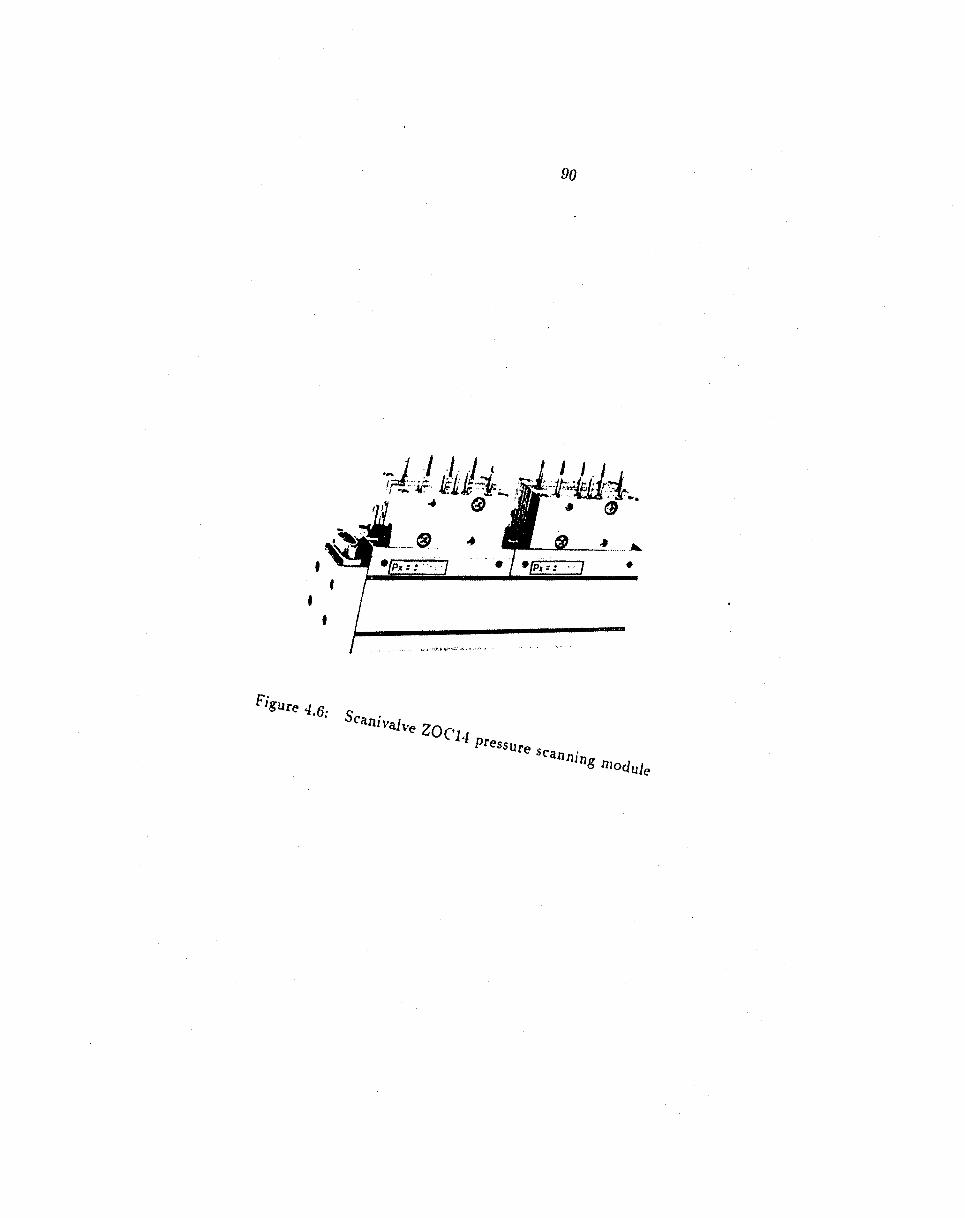
90

sèd'àllk

IPX = : • /

Fj

sfaon. niodu/g

91

tuai test scanning rates, however, were significantly lower because of the limitations

imposed by the Hewlett-Packard 3495A scanner that was used.

The Z0C14 is capable of four modes of operation: operate, calibrate, purge and

isolate. Each of these modes can be activated by applying an appropriate pneumatic

control pressure ( % 90 psi) to the Z0C14 module. The normal operating mode of the

Z0C14 is the "operate" mode. The 32 individual pneumatic pressures are sensed and

converted to voltage signals in this mode. The "calibrate" mode allows for the cali

bration of each individual sensor with some known calibration pressure. This mode

allows the Z0C14 sensors to be automatically calibrated on-line without interrupting

the test run. The last two modes of operation of the Z0C14 are the "purge" and

"isolate" modes. These modes purge impurities which may be introduced through

the pneumatic pressure lines and isolate the ZOC' from any pneumatic pressures.

For the Z0C'14 module to operate consistently and accurately, the entire unit was

installed in a Scanivalve Thermal Control Unit (TCLI, see Figure 4.7). The TCIU was

designed to provide a constant temperature environment for the Z0C14 scanning

module. The ZOC TCU minimizes the need to frequently recalibrate the silicon

pressure sensors because of exposure to varying ambient temperatures. By use of a

thermostatically controlled heater housed in a well insulated enclosure, temperature

changes within the Thermal Control Unit were less than 0.1°C from a nominal factory

setpoint temperature of 40°C.

The final piece of support equipment for the Scanivalve Z0C14 pressure scanning

module was a Scanivalve Mux Address Control Unit (MACU, see Figure 4.8). The

ZOC MACU is a compact address control unit that is capable of generating an address

stream based on commands from the data acquisition system. The MAC'U displays

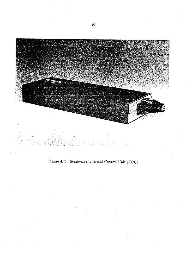
Figure 4.7: Scanivalve Thermal Control Unit (TCU)

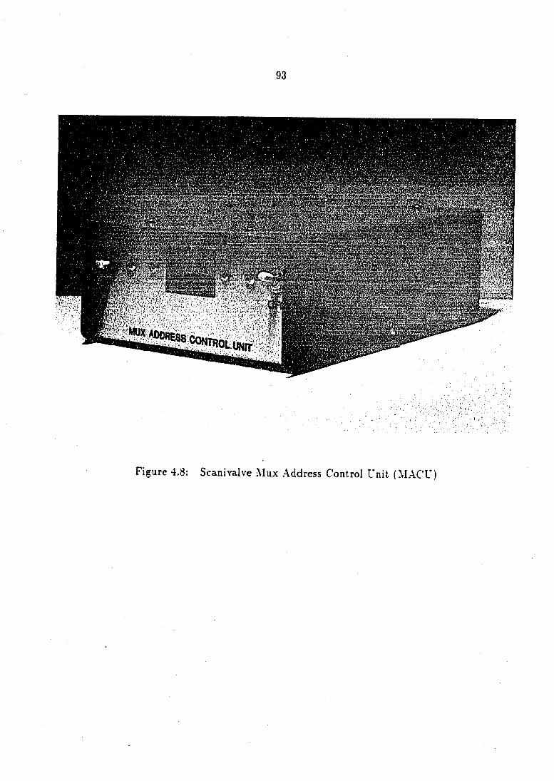
93

###

Figure 4.8: Scanivalve Mux Address Control Unit (MACU)

94

the current pressure channel being monitored and sends back a binary string code to

the data acquisition system for channel verification.

4.2.1.1 Pressure system setup and electrical diagram The system setup

and electrical diagram for the entire pressure scanning system are described in this

subsection. The three Scanivalve ZOC components, namely, pressure sensor mod

ule, thermal control unit and mux address control unit, were supplied with required

voltage sources and wired into existing laboratory data acquisition equipment.

The identification of required power supplies was the first step in the design of the

pressure system control logic. Each component of the Scanivalve pressure scanning

system required a different power supply as listed in Table 4.4. The power supplies

were mounted on a steel plate attached to a 19 in. rack mounted panel for use in

a portable rack enclosure. In addition to the power supplies, the control panel also

contained the electronics and hardware for operating in the four different pressure

scanning modes (operate, calibrate, purge and isolate). To operate in each of these

four modes, a 90 psi pneumatic control pressure was applied to two different control

pressure connections as indicated in Table 4.5.

The control panel housed two Asco 120 volt A. C., 2-way red-hat solenoid valves

for applying the control pressure as needed. Control logic for the four different modes

of operation was designed so that a red light was illuminated indicating which mode

of operation was in effect. series of -+-24 VDC relays and indicator lights were used

to accomplish this result. The schematic for the control pressure solenoid activation

and corresponding indicator lights is shown in Figure 4.9. The four different modes

of operation could be activated by the appropriate switching (on-off) of two 24 volt

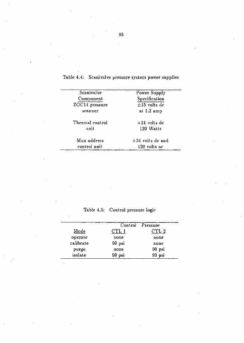
95

Table 4.4: Scanivalve pressure system power supplies

Scanivalve Power Supply Component Specification

Z0CU4 pressure ±15 volts dc scanner at 1.2 amp

Thermal control + 24 volts dc unit 120 Watts

Mux address + 24 volts dc and control unit 120 volts ac

Table 4.5: Control pressure logic

Control Pressure Mode CTL 1 CTL 2

operate none none calibrate 90 psi none

purge none 90 psi isolate 90 psi 90 psi

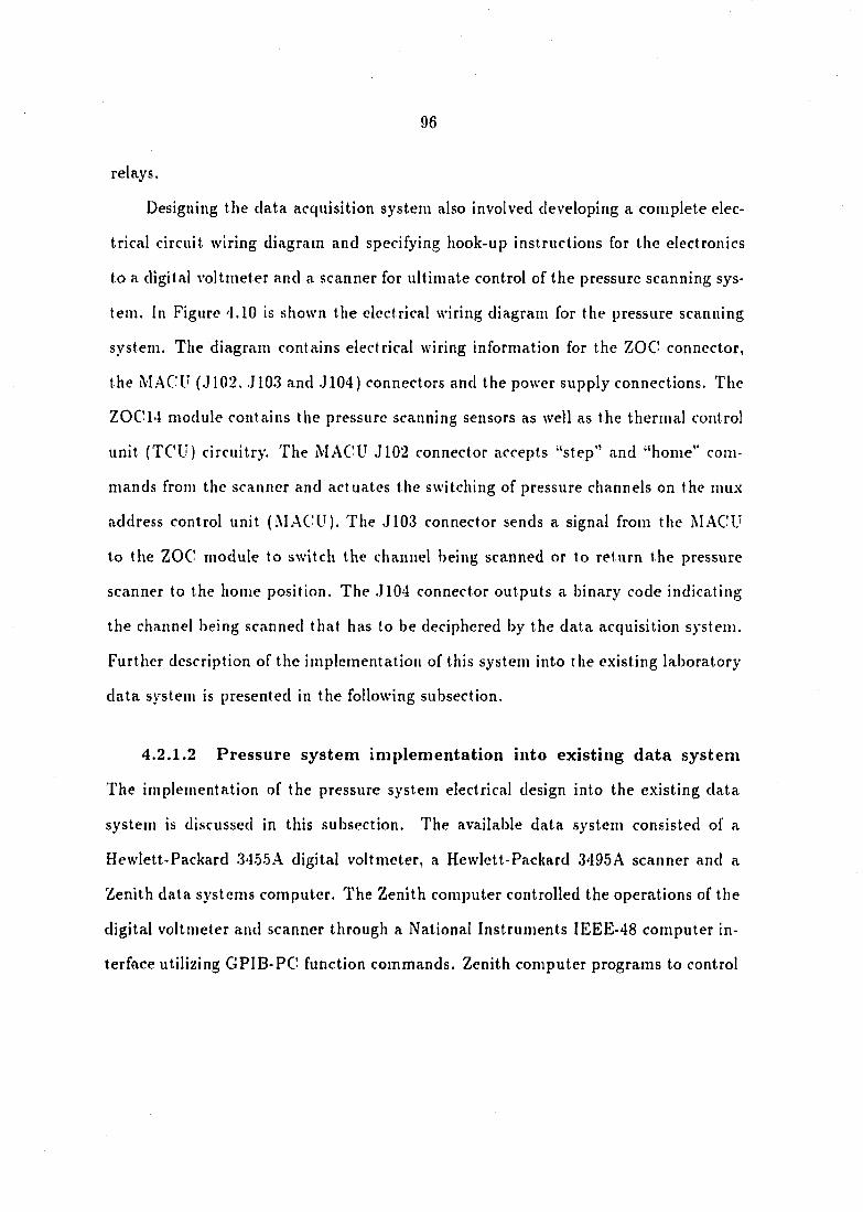
96

relays.

Designing the data acquisition system also involved developing a complete elec

trical circuit wiring diagram and specifying hook-up instructions for the electronics

to a digital voltmeter and a scanner for ultimate control of the pressure scanning sys

tem. In Figure 4.10 is shown the electrical wiring diagram for the pressure scanning

system. The diagram contains electrical wiring information for the ZOC connector,

the MACU (J102, J10.3 and J104) connectors and the power supply connections. The

Z0C14 module contains the pressure scanning sensors as well as the thermal control

unit (TCU) circuitry. The MACU J102 connector accepts "step" and "home'" com

mands from the scanner and actuates the switching of pressure channels on the mux

address control unit (M.ACU). The J103 connector sends a signal from the MACU

to the ZOC module to switch the channel being scanned or to return the pressure

scanner to the home position. The .1104 connector outputs a binary code indicating

the channel being scanned that has to be deciphered by the data acquisition system.

Further description of the implementation of this system into the existing laboratory

data system is presented in the following subsection.

4.2.1.2 Pressure system implementation into existing data system

The implementation of the pressure system electrical design into the existing data

system is discussed in this subsection. The available data system consisted of a

Hewlett-Packard 34.5.5A digital voltmeter, a Hewlett-Packard 3495A scanner and a

Zenith data systems computer. The Zenith computer controlled the operations of the

digital voltmeter and scanner through a National Instruments IEEE-48 computer in

terface utilizing GPIB-PC function commands. Zenith computer programs to control

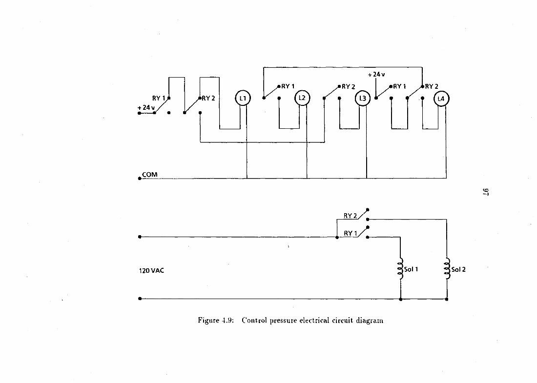
RY1,

+ 24v .

kRY2 © • RY1 ,#RY2 yRY 1 iRY2

< » r j i if M

COM

<o

«Y2/I

-._5r!/l

120 VAC So l i 4 Sol 2

Figure 4.9: Control pressure electrical circuit diagram

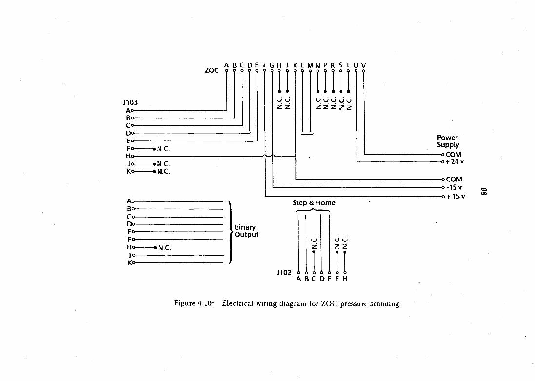
1103 Ao— Bo-Co-Do-Eo-Fo-Ho-Jo— Ko-

Ao-Bo-Co-Do-Eo-Fo-Ho-Jo-Ko-

A B C D E F G H J K L M N P R S T U V ZOC 99????9<7999(7<79Q999Q

• N.C.

-#N.C. -#NC

V u z z

U U U U V z z z z z

'N.C

Step & Home

Binary 'Output

o z

u u z z

J102 ÔÔÔÔÛÔÛ A B C D E F H

Power Supply

-oCOM —o + 24 V

-oCOM -o -15 V -o+ 15 V

CO oo

Figure 4.10; Electrical wiring diagram for ZOC pressure scanning

99

the function of the data acquisition system were written in Quick Basic language.

Two major operations were used to implement the Scanivalve pressure system

into the available data system, namely, reading and logging dc voltages from the

digital voltmeter and controlling relay switches on the scanner. By using these oper

ations, the Z0C14 pressure scanner could be stepped and homed, the ZOO output

voltage could be read, and the binary code produced by the MACU could be deci

phered. These important pressure system operations will be discussed briefly.

First of all, the "'step'" and ''home" commands were created by the sequential

opening and closing of two scanner relays. The '"step" operation caused the ZOC'

channel being scanned to be incremented by one channel (or pneumatic pressure in

put). The "home" operation caused the ZOC scanner to return to its initial scanning

position (Channel 0). The scanning rate of the system was limited by the speed at

which the scanner relays could be opened and closed. The maximum scanning speed

used for data acquisition purposes was about eight channels per second (== 8 Hz). A

simple sketch of the scanner electrical hook-up for the step and home operations is

shown in Figure 4.11. A step is accomplished by opening and closing switch 1 (SW

1) followed by closing switch 2 (SW 2). A home command is accomplished by closing

switch .3 (SW .3). The scanner automatically reopens a switch when a new command

is given to open or close an alternate switch.

The second important operation for the data system was the reading of the

ZOC 14 output voltage. The dc voltage was read by the digital voltmeter (wires L

and M in Figure 4.10). This dc voltage was directly proportional to the pressure

being applied to the individual silicon sensor. Each sensor, however, had a different

proportionality constant associated with it. The method of calibration of these silicon

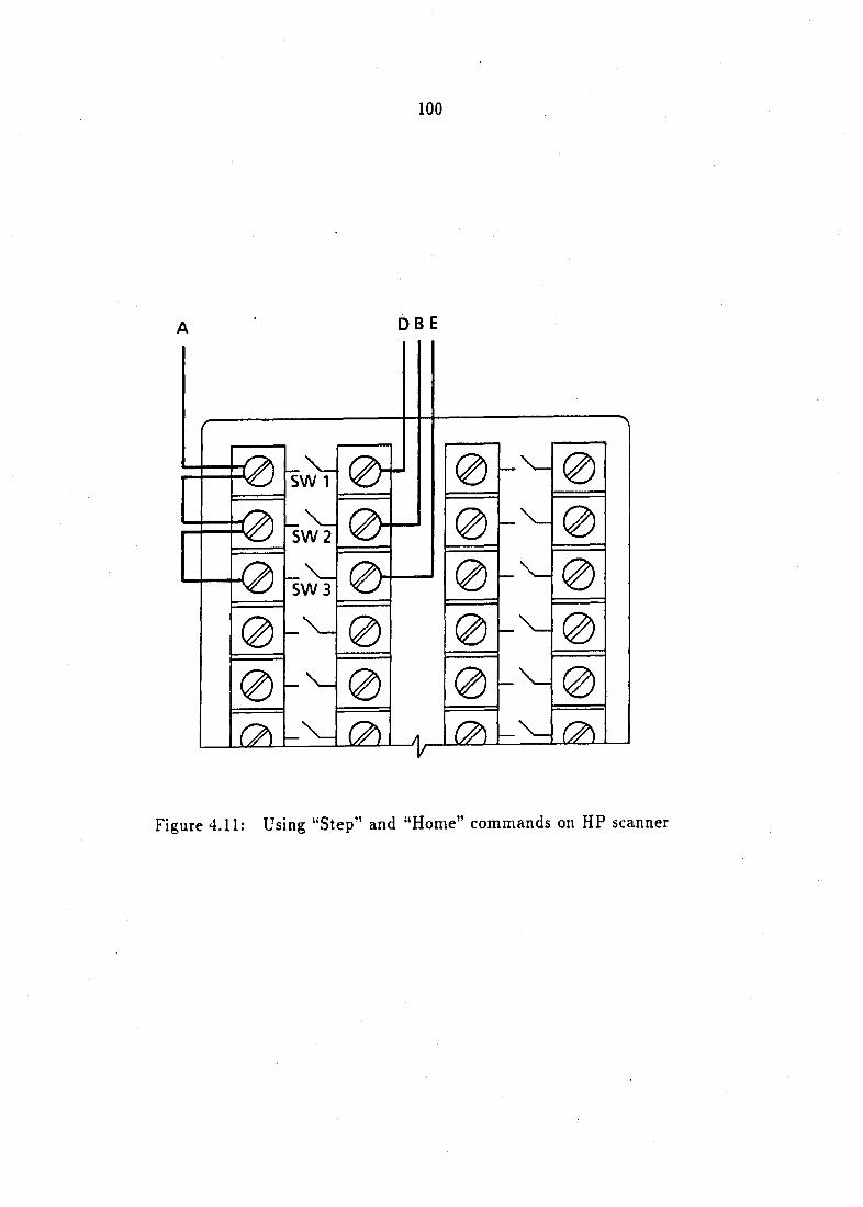
100

DB E

i2L

SW 1

SW2

SW3

0-^

0—'

4-m m

Figure 4.11: Using "Step" and "Home" commands on HP scanner

101

pressure sensors is discussed in the pressure system calibration subsection.

The deciphering of the binary code produced by the ZOC MACU was the final

pressure system operation. The deciphering of this code enabled the data system

to verify the channel being scanned. The binary code string flowed from connector

J104 on the MAC'U. The connector contained six open collector NPN transistors

with a maximum saturation voltage of 0.5 volts when "on". An external 24 volt dc

power supply was required for the deciphering operation. In Figure 4.12 is shown the

six NPN transistor connectors labeled A through F. Each connector has a different

binary number associated with it and they are indicated in the diagram.

The diagram shows a parallel arrangement of pull-up resistors and a voltmeter

which must be examined for deciphering purposes. Each circuit voltage (A through

F) must be read and recorded. The resulting voltage values reflect either an "on" or

"off' condition for the NPN transistors. The channel being scanned is calculated by

adding the binary numbers of the NPN transistors which indicate an "off" condition.

4.2.1.3 Pressure system calibration The calibration procedure for the

Scanivalve ZOC 14 pressure scanner is discussed in this subsection. The ZOC 14 pres

sure module contained 32 individual silicon sensors each having a different calibration

constant. Each sensor had a nominal differential pressure range of 10 psi, and was

therefore calibrated in this range. A seven point calibration for each of the 32 indi

vidual sensors was performed.

The calibration involved a small air compressor and a 30 inch mercury manome

ter. The air compressor provided a variable pressure source in the 0 to 10 psi range.

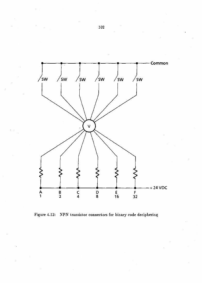
102

Common

Figure 4.12: NPN transistor connectors for binary code deciphering

103

The mercury manometer was used to measure precisely the pressure of the variable

source.

The calibration procedure began by switching on the pressure system electronics.

A two hour warm-up time was required for the thermal control unit (TCU) to reach

thermal equilibrium. Because the silicon sensors were sensitive to thermal gradients,

a calibration performed before the system was stable yielded erroneous results. When

the pressure measuring system was in equilibrium, a scan of the 32 individual sensors

indicated a non-zero initial voltage for each. This initial voltage was most likely

due to stresses applied to each silicon sensor during manufacturing and it remained

constant throughout the calibration and during subsequent testing.

Seven nominal pressure source values were chosen for calibration, namely, 0.0,

2.0, 4.0, 5.0, 6.0, 8.0 and 10.0 psi. The calibration pressure was applied to each

of the silicon pressure sensors and voltage readings were taken. This process was

repeated with the remaining calibration pressures to arrive at calibration curves for

each of the 32 sensors. This calibration procedure was then repeated immediately

to verify that the calibration curves remained constant. In Figure 4.13 is shown the

calibration curve for channel number 24 of the Z0C14. Other calibration curves for

the remaining ZOC channels were similar with different slopes, however. The slope of

the calibration curve of voltage versus pressure gives the calibration constant. Table

4.6 lists the calibration constants calculated for the 32 individual silicon pressure

sensors. During the Pratt & Whitney compressor tests, calibration constants were

checked periodically and did not vary.

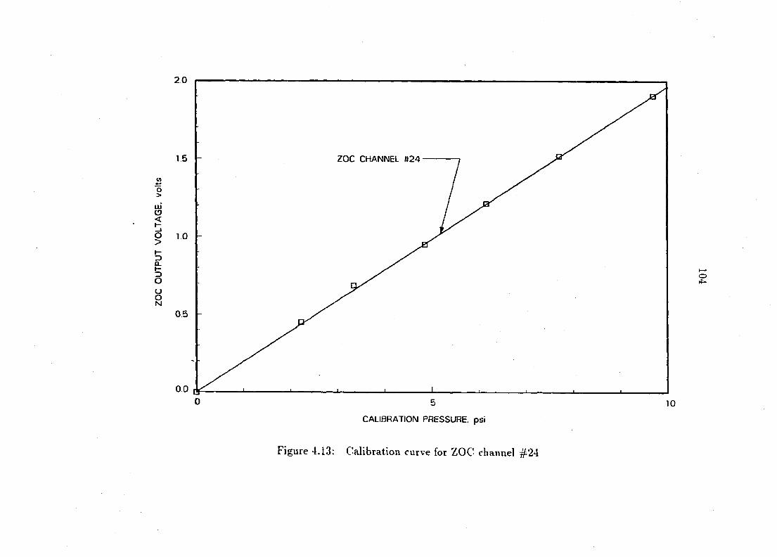
20

15 ZOC CHANNEL «24

«

o > Ul o < h-d >

3 a 3 O

05

0 0 0 5 10

CALIBRATION PRESSURE, psi

Figure 4.13: Calibration curve for ZOC channel #24

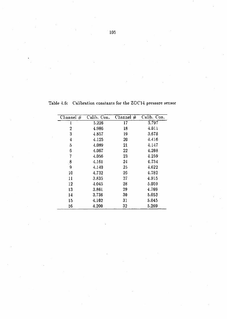
105

Table 4.6: Calibration constants for the Z0C14 pressure sensor

C'hannel # Calib. Con. Channel # Calib. Con. I 5.226 17 3.797 2 4.986 18 4.011 3 4.857 19 3.678 4 4.125 20 4.416 5 4.089 21 4.147 6 4,067 22 4.208 7 4.056 23 4.259 8 4.161 24 4.734 9 4.140 25 4.622

10 4.732 26 4.782 11 3.8.35 27 4.915 12 4.045 28 5.059 13 3.861 29 4.769 14 3.736 30 5.053 15 4.102 31 5.045 16 4.200 32 5.269

106

4.2.2 Temperature system

The temperature data acquisition system used with the intermediate-speed,

three-stage, axial-flow compressor is described in this subsection. The tempera

ture measurement system consisted of chromel-alumel thermocouples attached to

total-temperature probes. Individual thermocouples were hooked-up to the Hewlett-

Packard 3495A scanner in a parallel arrangement. The scanning of up to 40 different

thermocouples was performed by the Zenith computer. ,An Omega-CJ cold junction

compensator was used to provide a reference point from which to base the thermocou

ple emf. The emf voltage was read by the Hewlett-Packard 3455A digital voltmeter.

Using the following equation provided by Omega, the thermocouple temperature was

calculated.

T — (IF) (I\X -f -f- ... + z" (4.1)

where

T = thermocouple absolute temperature

J = thermocouple emf voltage

a = polynomial coefficient for chromel-alumel thermocouple

m = maximum order of the polynomial

In this case, an 8''* order polynomial was used to calculate the thermocouple tem

perature. The polynomial coefficients for a Type K, chromel-alumel thermocouple are

tabulated below. This 8'' ' order polynomial resulted in a thermocouple temperature

accuracy of ± 0.7°. The values of polynomial coefficients used are:

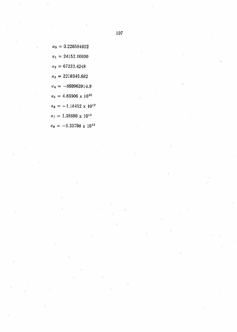
ao = 0.226584602

ai = 24152.10900

02 = 6723.3.4248

«3 = 2210340.682

«4 = -860963914.9

as = 4.83506 x 10'°

«6 = -1.184.52 X 10'-

«- = 1.38690 X 10'3

ag = —6.33708 x 10'

108

4.3 Pratt & Whitney Three-Stage Compressor Performance Tests

The Pratt & Whitney, intermediate-speed, three-stage compressor was used for

the purpose of identifying the effects of compressibility on the proposed method

for improving the stall margin of multistage, axial-flow compressors. The results

previously obtained with the two-stage fan and the three-stage compressor were used

to guide the Pratt &: Whitney compressor tests. Because the Pratt & Whitney

compressor was a significantly more complex turbomachine than the two-stage fan

and three-stage compressor, the test procedures are explained in detail.

The overall performance characteristics for the Pratt & Whitney, intermediate-

speed, three-stage, axial-flow compressor were determined by the measurement of

inlet corrected mass flow, compressor total-pressure rise and inlet corrected rotational

speed. These performance parameters were carefully measured throughout the test

program to assure accurate and consistent results. The methods used to determine

these performance parameters are discussed in the following sections.

4.3.1 Inlet corrected mass flow

The flow rate for the Pratt & Whitney compressor was measured in an instru

mented annulus section located downstream of the compressor exit (see Figure 4.3).

The measurement section could be easily separated from the compressor assembly

without dismantling the entire compressor. The flow rate measurement section had

an inside diameter of 20.59 inches and an outside diameter of 24.00 inches, resulting

in a 1.70 inch passage height. Four specially designed probe holders were manufac

tured and installed at four locations around the measurement section circumference.

The probe holders were designed to hold total-pressure and total-temperature probes

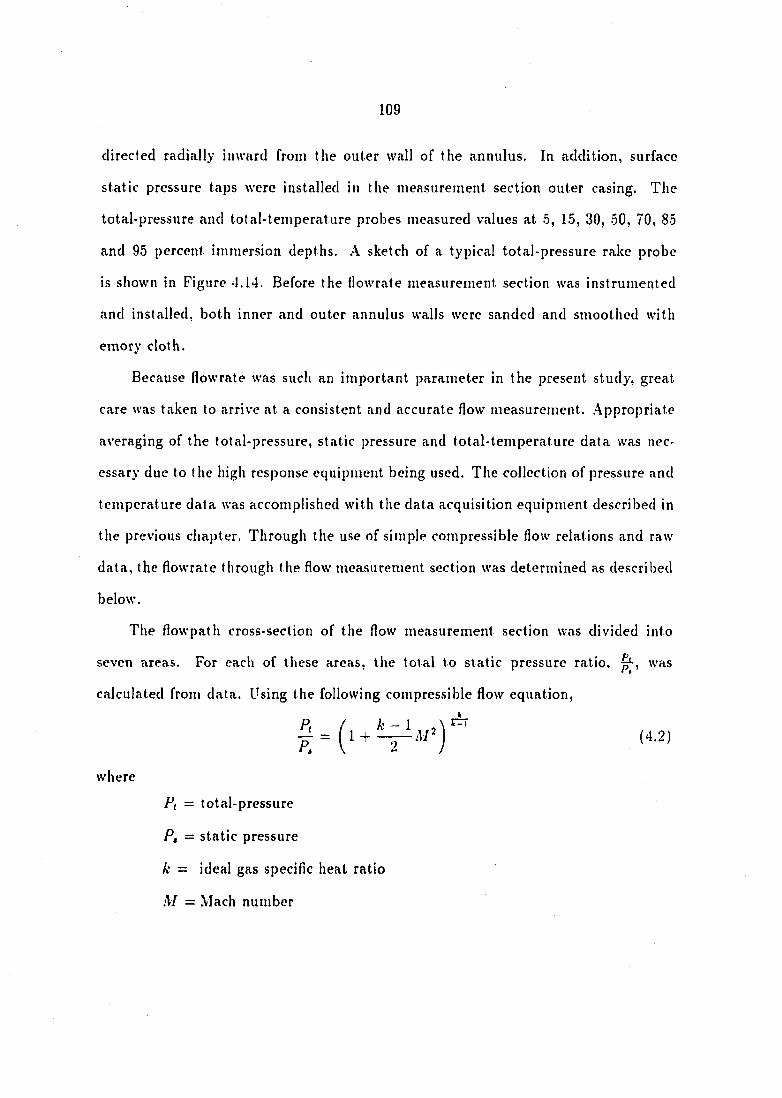
109

directed radially inward from the outer wall of the annulus. In addition, surface

static pressure taps were installed in the measurement section outer casing. The

total-pressure and total-temperature probes measured values at 5, 15, 30, 50, 70, 85

and 95 percent immersion depths. A sketch of a typical total-pressure rake probe

is shown in Figure 4.14. Before the flowrate measurement section was instrumented

and installed, both inner and outer annulus walls were sanded and smoothed with

emory cloth.

Because flowrate was such an important parameter in the present study, great

care was taken to arrive at a consistent and accurate flow measurement. Appropriate

averaging of the total-pressure, static pressure and total-temperature data was nec

essary due to the high response equipment being used. The collection of pressure and

temperature data was accomplished with the data acquisition equipment described in

the previous chapter. Through the use of simple compressible flow relations and raw

data, the flowrate through the flow measurement section was determined as described

below.

The flowpath cross-section of the flow measurement section was divided into

seven areas. For each of these areas, the total to static pressure ratio, was

calculated from data. Using the following compressible flow equation,

(4.2)

where

Ft = total-pressure

P, = static pressure

k = ideal gas specific heat ratio

M = Mach number

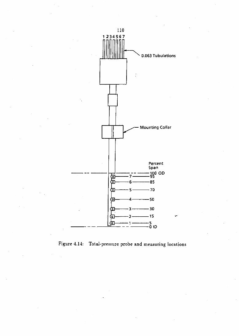
110

0.063 Tabulations

Mounting Collar

Percent Span

-100 OD

0 ID

Figure 4.14: Total-pressure probe and measuring locations

Ill

We can obtain the following relationship for the Mach number, M,

= \llh{p.) ' (4.31

With the total to static pressure ratio known, the Mach number can be calculated

with Equation (4.3). From the following compressible flow equation,

l + ( 4 . 4 )

where

Tt = total-temperature

T = static temperature

the static temperature. T, can be evaluated with

= TTW

The velocity, I'', of the air can be calculated using the definition of Mach number,

V = ( 4 . 6 )

where

l' = absolute fluid velocity

R = molecular weight

The flowrate, rfi, can be calculated using the following equation

j'n = pAV (4.7)

and the ideal gas relation

P = pRT (4.8)

112

Then the How rate is given by

PVA m = (4.9)

Using the above stated equations, the flowrates for each of the seven areas and

for data from each of the four circumferential locations were evaluated. The final

overall flowrate was calculated by averaging the four different circumferential position

flowrates for each of the seven different flow passage areas.

The data acquisition program was written to scan total-pressures, static pres

sures and total-temperatures five times and average them before calculating the in

dividual passage flowrates. The program calculated the total compressor flowrate

every minute. To arrive at a final measurement for the flowrate, the results of five

individual mass flowrate runs were averaged.

Having obtained the mass flowrate, the equation for inlet corrected mass flow is

given by

(4.10) in le t

where

m = mass flowrate

Û total température at compressor inlet ' ~ sea level standard temperature

g total pressure at compressor inlet ' sea level standard pressure

The quantities Ot and 6, were calculated by using measured values of total tem

perature and pressure at the compressor inlet. This was accomplished by using

a midspan total-temperature and total-pressure probe positioned upstream of the

compressor inlet.

113

4.3.2 Compressor pressure rise ratio

The second overall performance parameter measured on the Pratt & Whitney

compressor test rig was compressor total-pressure rise ratio. The compressor total-

pressure rise ratio is given by

(4.11) n.in/et

where

Pt .outut = compressor outlet total-pressure

Pf.inUt = compressor inlet total-pressure

In addition to this total pressure parameter, the compressor static pressure rise

ratio was also evaluated. The method for collecting the data for these ratios is

explained briefly in this subsection.

The total-pressure rise across the compressor was measured using two total-

pressure probes located at the inlet and exit of the compressor. The probes were

total-pressure rakes which measured the total-pressure from 1.5 percent to 85 percent

immersion depths. Five total-pressure measurements at 15, 30, 50, 70 and 85 percent

immersion were averaged to arrive at the inlet or exit total-pressure measurement.

A .Meriam 30 inch column of mercury was used to measure the total-pressure read

ings. The barometric pressure was measured with a Fisher Scientific Model #0284

barometer.

Compressor static pressure rise was measured with static pressure tap holes

located at the inlet and exit of the compressor. The mercury manometer was used

to measure the static pressure readings.

114

4.3.3 Inlet corrected rotational speed

The final overall compressor performance parameter measured on the Pratt &

Whitney compressor was inlet corrected rotational speed. The equation for inlet

corrected rotational speed is

(4.12) inlet

where

RPM •— rotor rotational speed

^ totnl-"température at compressor inlet sen leve l s tandard temperature

This equation indicates that a changing compressor inlet condition will affect the

inlet corrected rotational speed. Because ambient air from the outside flowed through

the compressor, it was important to closely monitor the inlet total-temperature and

make any necessary adjustments in the rotor rotational speed to keep the inlet cor

rected rotational speed constant. Over the course of a data run, these adjustments

had to be made fairly frequently. The total-temperature probe positioned at the

compressor inlet was used to monitor the compressor inlet total-temperature. The

compressor rotor rotational speed was measured with a tachometer mounted on the

compressor drive motor.

4.3.4 Detection of stall in the Pratt & Whitney compressor

The method for detection of stall in the Pratt & Whitney compressor is discussed

in this subsection. careful and systematic approach was used to establish a consis

tent and accurate representation for operating points on the compressor surge/stall

limit line.

115

Stall tests were performed by slowly reducing the inlet corrected mass flow along

a constant inlet corrected rotational speed line. The mass flow reduction was ac

complished by moving the cone shaped compressor throttle axially. Each movement

of the throttle was indicated by a digital readout located on the compressor con

trol panel. When the compressor operated near stall, measurements were taken for

determining the overall compressor performance parameters. These measurements

were recorded and the throttle was moved to further reduce the mass Howrate. This

process continued until the sound of operation of the compressor changed distinctly

because of stall. The measurements of flowrate and total-pressure rise taken just

before the compressor became unstable were considered to be for the stall point op

erating conditions. This process for detecting stall along a constant inlet corrected

rotational speed line was repeated four to five times in a data run. The stall tests

were also repeated on subsequent days to verify the consistency and repeatability of

the results. Data for several constant speed lines were obtained. Because stall point

data were consistent throughout a data run and did not vary significantly from run

to run or from day to day, it was felt that the error band for these measurements was

within the symbol used.

5. ESTIMATION OF REDUCED FREQUENCY AND ROTOR

INLET FLOW ANGLE VARIATION FOR PRATT & WHITNEY

COMPRESSOR

In the absence of detailed flow measurements (velocity magnitude and flow angle)

for the flow entering a rotor row, an estimate of the reduced frequency at stall,

and an estimate of the rotor inlet flow angle variation must be made. For a

given number upstream stationary blade of setting angle variation cycles per rotor

revolution, n, and a given amplitude of setting angle variation, Afji, these estimates

are required to choose baseline compressor modifications which may show benefit in

terms of stall margin improvement. A thorough analysis of this estimation process for

the two-stage axial-flow fan and the three-stage axial-flow compressor was presented

in reference [12j. The estimation process for the Pratt & Whitney, intermediate-

speed, three-stage, axial-flow compressor for each of the six inlet corrected rotational

speeds tested is outlined in detail below.

Flow conditions at the exit of the inlet guide vane (IGV) row give the magnitude

of the absolute velocity approaching the rotor. This velocity is necessary to calculate

the fluid relative velocity at the rotor inlet used in estimating the reduced frequency

at stall, K,taih The technique for calculating the reduced frequency involves using

global flow parameters, simple blade row geometry, and a well accepted correlation

117

of blade deviation angle to arrive at a reasonable estimate of the reduced frequency

at stall. The steps used in calculating the reduced frequency at stall for the Pratt &

Whitney compressor are summarized below:

1. Determine the midspan average axial velocity at stall using the mass flowrate at stall.

2. Estimate the midspan flow deviation angle behind the inlet guide vane (IGV) row.

3. Draw velocity triangles at midspan using simple blade row geometries.

4. Calculate the magnitude of the midspan fluid relative velocity at rotor inlet.

5. Use Equation (3.5) to calculate h'siaii-

The material in references [12] and [14] suggests that the magnitude of the rotor

inlet flow angle variation may be significantly difl'erent from the magnitude of the

blade setting angle variation prescribed for the stationary row upstream of the rotor.

An estimate of this difference is necessary to completely describe the effect of the inlet

guide vane setting angle variation. A. detailed analysis of the first stage rotor inlet

flow angle variation for the Pratt & Whitney compressor is described in the following

sections. A portion of the analysis for the three types of inlet guide vane row blade

setting angle patterns used in the low-speed, three-stage, axial-flow compressor taken

from reference [12] is also summarized. Those three inlet guide vane row setting

angle patterns were sinusoidal (Equation 3.1), rectified sine-wave (Equation 3.2) and

asymmetric (Equation 3.3) variations.

The following two sections outline the procedure for calculating the reduced

frequency at stall, K,ta ih and the extent of rotor inlet flow angle variation for the

Pratt & Whitney compressor.

118

5.1 Calculation of Reduced Frequency at Stall, K,taih for the Pratt &:

Whitney Compressor

The estimation of the reduced frequency at stall, Kataih for the Pratt & Whitney

compressor involved an evaluation of the stalling mass flowrate. Performance tests

were conducted at each of the six inlet corrected rotational speeds, namely, 50, 60,

70, 80, 90 and 100 percent of design speed. Repetition of tests at the stall condition

for each of these speeds resulted in the stall point overall mass flowrate conditions.

These performance points are the actual stall/surge point limits shown in Figure 6.1.

Using the following equation, the axial velocity at the stall condition for each speed

was calculated.

— PinUt inlet (5.1)

where

m = compressor stalling mass flowrate

pinitt = fluid density at compressor inlet

Air,ut = annul us area at compressor inlet

Kn/e( = axial velocity at compressor inlet

In Table 5.1 are summarized values of the stalling mass flowrate and the axial

velocity at stall for each of the six inlet corrected rotational speeds.

Before the blade velocity diagrams can be constructed, a reasonable estimate of

the inlet flow angle involved must be made. This estimate is made by using simple

blade row geometry and a correlation for blade deviation angle given by Carter [15].

Summarized below are some important inlet guide vane midspan blade row angles

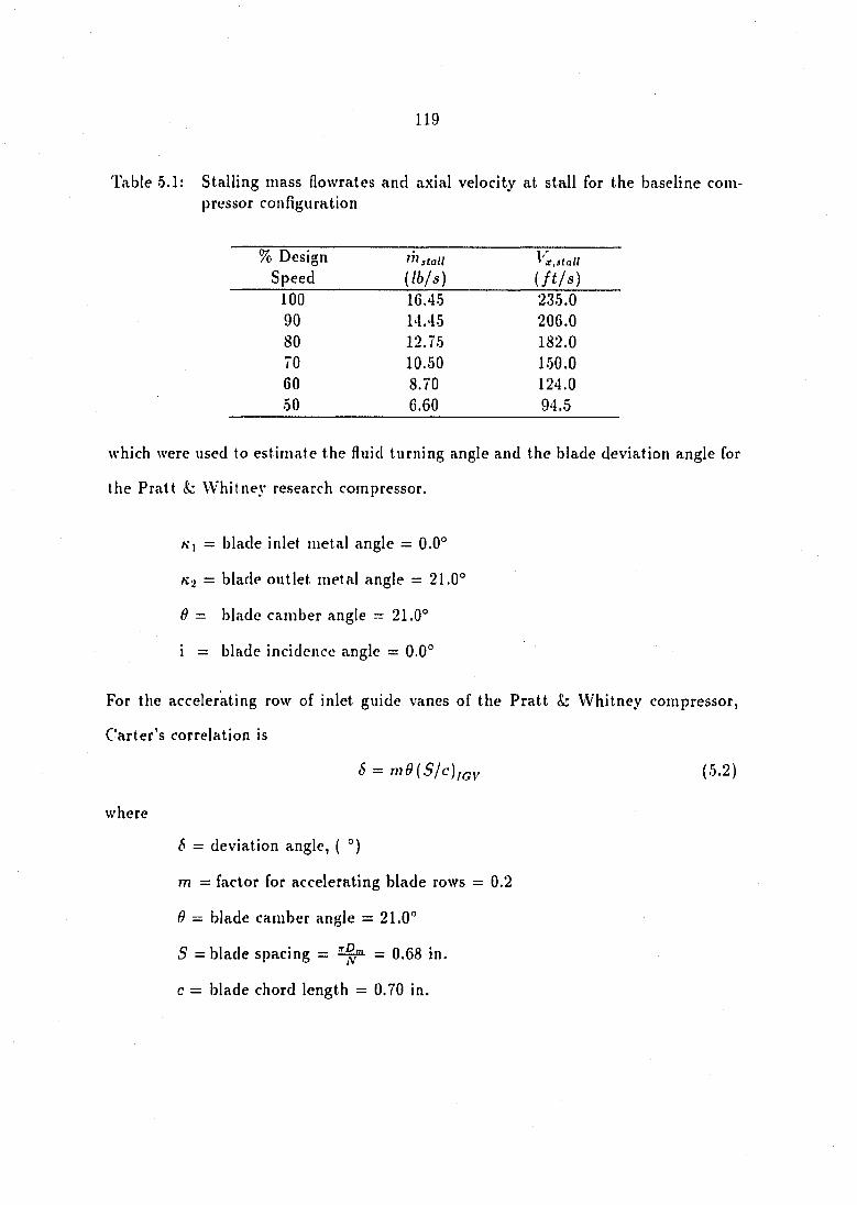
119

Table 5.1: Stalling mass flowrates and axial velocity at stall for the baseline compressor configuration

% Design s ta l l s ta l l

Speed (/6/j) i f t / s ) 100 16.4.5 235.0 90 14.45 206.0 80 12.75 182.0 70 10.50 150.0 60 8.70 124.0 .50 6.60 94.5

which were used to estimate the fluid turning angle and the blade deviation angle for

the Pratt & Whitney research compressor.

Ki — blade inlet metal angle = 0.0°

Ki = blade outlet metal angle = 21.0°

6 — blade camber angle — 21.0°

i = blade incidence angle = 0.0°

For the accelerating row of inlet guide vanes of the Pratt & Whitney compressor,

Carter's correlation is

S = m d ( S l c ) j Q y (.5.2)

where

8 = deviation angle, ( °)

m = factor for accelerating blade rows = 0.2

9 = blade camber angle = 21.0°

S = blade spacing = = 0.68 in.

c = blade chord length — 0.70 in.

120

With Equation (5.2) and these quantities, the midspan, inlet guide vane deviation

angle was estimated to be

a =5 4.0° (5.3)

Using this blade deviation angle and the following equations, the rotor inlet flow

velocity diagrams at stall for the Pratt & Whitney compressor at each of the six inlet

corrected rotational speeds were constructed.

cio — .'^2 — 6 (5.4)

t m . a n - g Q Q

I'M = I': tan Ag (5.6)

W29 = Vmran " (5.7)

W2 = yj ujg + v.- (5.8)

/jg = arctan ( ) (5.9)

These calculations are all based on the mean radius of the research compressor, which

is calculated as

rm = (r„p + r uk) (5.10)

In Table 5.2 are summarized some of the results of the velocity diagram calcula

tions for the Pratt & Whitney baseline compressor configuration at stall. Summarized

are the absolute tangential velocity, V29, the mean blade velocity, Umeani the relative

tangential velocity, lu;*, the relative velocity, wz and the relative flow angle,

In Figures 5.1 through 5.6 are illustrated the first stage rotor inlet flow velocity

triangles for the Pratt & Whitney compressor at the stall point for each of the inlet

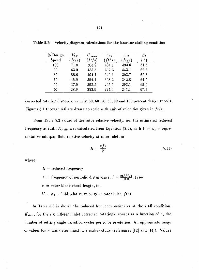
121

Table 5.2: Velocity diagram calculations for the baseline stalling condition

% Design ^^mean W29 W2 1^2 Speed ( f t / ' s ) (/f/a) (/f/a) i f t / s ) ( °)

100 00

505.9 434.1 493.6 61.6 90 63.0 455.3 392.3 443.1 62.3 80 55.6 404.7 349.1 393.7 62.5 70 45.9 .354.1 308.2 342.8 64.0 60 37.9 303.5 265.6 293.1 65.0 50 28.9 252.9 224.0 243.1 67.1

corrected rotational speeds, namely, 50, 60, 70, 80, 90 and 100 percent design speeds.

F i g u r e s 5 . 1 t h r o u g h 5 . 6 a r e d r a w n t o s c a l e w i t h u n i t o f v e l o c i t i e s g i v e n i n f t / s .

From Table 5.2 values of the rotor relative velocity, us, the estimated reduced

frequency at stall, h'TTAII, \^'As calculated from Equation (3.5), with V = TVO = repre

sentative inidspan fluid relative velocity at rotor inlet, or

A ' = ~ ( 5 . 1 1 )

where

K = reduced frequency

/ = frequency of periodic disturbance, / = 1/sec

c = rotor blade chord length, in.

V = W 2 = fluid relative velocity at rotor inlet, f t / s

In Table 5.3 is shown the reduced frequency estimates at the stall condition,

for the six different inlet corrected rotational speeds as a function of n, the

number of setting angle variation cycles per rotor revolution. An appropriate range

of values for n was determined in a earlier study (references [12] and [14]). Values

122

Table 5.3: Reduced frequency at stall, for the Pratt & Whitney three-stage axial-flow compressor

Percent Speed

Reduced frequency at Stall, stall

100 0.094n 90 0.094n 80 0.0947! 70 0.09-57?

60 0.095n 50 0.096n

for A',(a// considered to have likelihood of benefit were in the range from 0.19 to 0.20.

Therefore, a 2/rev variation (n = 2) in setting angle was considered appropriate for

the Pratt & Whitney compressor.

123

67.1 17.0 LO

m 224.0

28.

236.3

Figure ô.l: Pratt & Whitney blade velocity diagram at stall for .50 percent speed

65.0' ,17.0

265.6 37.

281.6

Figure 5.2: Pratt & Whitney blade velocity diagram at stall for 60 percent speed

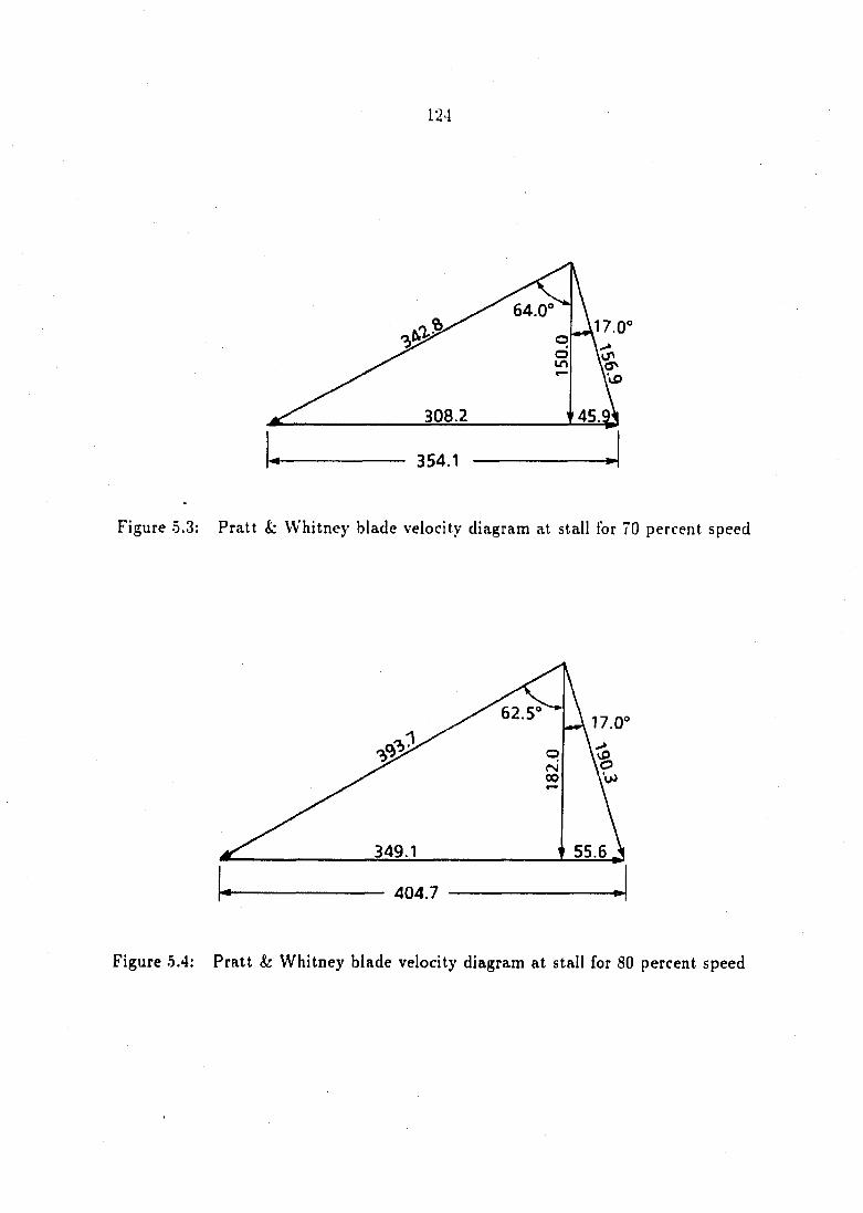
124

64.0 17.0

o

m

308.2 "45.

354.1


62.5 17.0

o (N 00

55.6 349.1

404.7


125

62.3 17.0

o

392.3 63.0

455.3


61.6 17.0

o

m CM

71.8 434.1

505.9 •


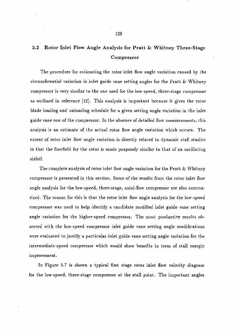
126

5.2 Rotor Inlet Flow Angle Analysis for Pratt &c Whitney Three-Stage

Compressor

The procedure for estimating the rotor inlet flow angle variation caused by the

circumferential variation in inlet guide vane setting angles for the Pratt & Whitney

compressor is very similar to the one used for the low-speed, three-stage compressor

as outlined in reference [12]. This analysis is important because it gives the rotor

blade loading and unloading schedule for a given setting angle variation in the inlet

guide vane row of the compressor. In the absence of detailed flow measurements, this

analysis is an estimate of the actual rotor flow angle variation which occurs. The

extent of rotor inlet flow angle variation is directly related to dynamic stall studies

in that the flowfield for the rotor is made purposely similar to that of an oscillating

airfoil.

The complete analysis of rotor inlet flow angle variation for the Pratt & Whitney

compressor is presented in this section. Some of the results from the rotor inlet flow

angle analysis for the low-speed, three-stage, axial-flow compressor are also summa

rized. The reason for this is that the rotor inlet flow angle analysis for the low-speed

compressor was used to help identify a candidate modified inlet guide vane setting

angle variation for the higher-speed compressor. The most productive results ob

served with the low-speed compressor inlet guide vane setting angle modifications

were evaluated to justify a particular inlet guide vane setting angle variation for the

intermediate-speed compressor which would show benefits in term of stall margin

improvement.

In Figure 5.7 is shown a typical first stage rotor inlet flow velocity diagram

for the low-speed, three-stage compressor at the stall point. The important angles

"28

U mean

Figure 5.7: Typical first stage rotor inlet flow velocity diagram at the stall point of the three-stage compressor

128

illustrated in the figure are, og, the flow angle at the inlet guide vane row exit, and

,62, the relative inlet flow angle perceived by the rotor blade. It is evident that as the

inlet guide vane row exit flow angle, «2, changes, due to changes in IGV row setting

angle, the relative inlet flow angle perceived by the rotor, dg, also changes. With the

shape of the velocity triangle involved, the change in /?2 is generally smaller than the

change in O;.

To estimate the change in relative flow angle, it is assumed that the change in

inlet guide vane row exit flow angle is identical to the blade setting angle increment

from baseline, A<p,. Earlier conclusions from low-speed compressor detailed mea

surement data suggest that this is a valid assumption. The corresponding change in

relative rotor inlet flow angle, d,, may then be estimated by constructing a new veloc

ity triangle where the axial velocity remains constant and is the baseline value. The

rotor inlet flow velocity diagrams of the baseline compressor (Figures 5.1 through 5.6

and Table 5.2) at the stall point defines the baseline values of, Oj, the IGV row exit

flow angle and iSi, the relative rotor inlet flow angle. The cjuantity, A/^j, represents

the difl'erence between the baseline rotor inlet relative flow angle and the modified

rotor inlet relative flow angle and is given by the following relation.

~ f^2,baatl ine ~ 1^2,modij ied (5.12)

where

fh.baseiine — Totor inlet relative flow angle for the baseline stalling condition

02,modified = TotoT inlet relative flow angle for the modified stalling condition

In Figures 5.8 and 5.9 are illustrated some of the results of the rotor inlet flow

angle analysis from the low-speed, three-stage compressor. Shown in Figure 5.8 is an

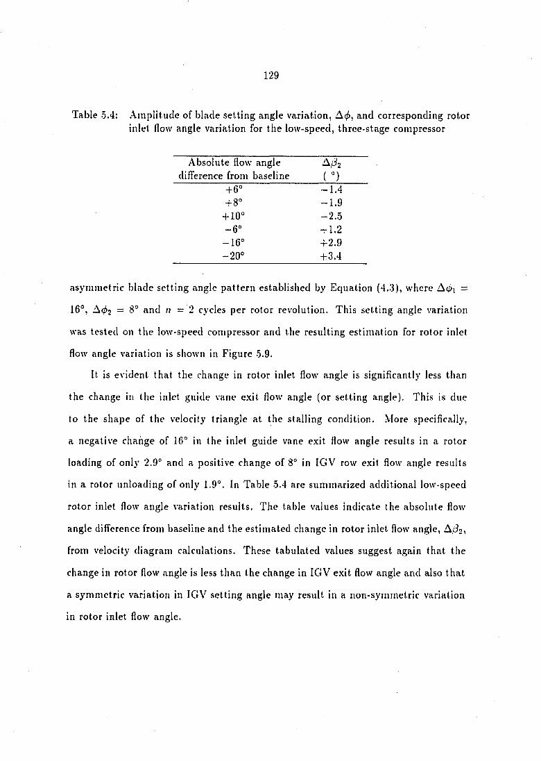
129

Table 5.4: Amplitude of blade setting angle variation, and corresponding rotor inlet flow angle variation for the low-speed, three-stage compressor

Absolute flow angle A/^2 difference from baseline ( °)

—

+8° -1.9 + 10° -2.5 -6° 4-1.2

-16° -f2.9 -20° +3.4

asymmetric blade setting angle pattern established by Equation (4.3), where Aéi =

16°, Aç!>2 = 8° and n - '1 cycles per rotor revolution. This setting angle variation

was tested on the low-speed compressor and the resulting estimation for rotor inlet

flow angle variation is shown in Figure 5.9.

It is evident that the change in rotor inlet flow angle is significantly less than

the change in the inlet guide vane exit flow angle (or setting angle). This is due

to the shape of the velocity triangle at the stalling condition. More specifically,

a negative change of 16° in the inlet guide vane exit flow angle results in a rotor

loading of only 2.9° and a positive change of 8° in IGV row exit flow angle results

in a rotor unloading of only 1.9°. In Table 5.4 are summarized additional low-speed

rotor inlet flow angle variation results. The table values indicate the absolute flow

angle difference from baseline and the estimated change in rotor inlet flow angle, A/^o,

from velocity diagram calculations. These tabulated values suggest again that the

change in rotor flow angle is less than the change in IGV exit flow angle and also that

a symmetric variation in IGV setting angle may result in a non-symmetric variation

in rotor inlet flow angle.

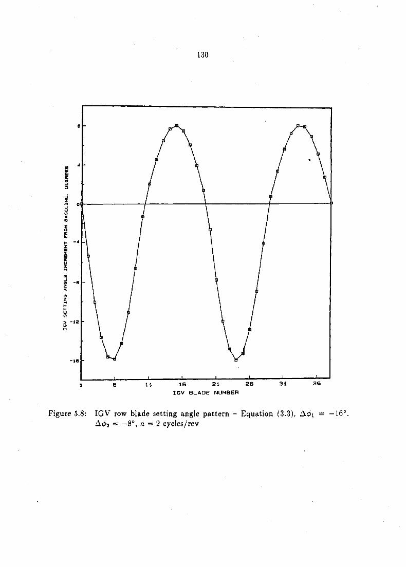
130

1 8 11 IB 21 2G 31 3B IGV BLADE NUMBER

Figure .5.8: IGV row blade setting angle pattern - Equation (3.3), Aôi = à.02 = —8°, n = 2 cycles/rev

131

M W UJ Œ 19 tu Q

W Z M J UJ U) 4 m z o s u.

UJ

é Z <

X o u u. #-tu i M r o o -8 cc B 16 26 31 1 1 21 36 1

IGV BLADE NUMBER

Figure 5.9: Estimated rotor inlet flow angle for Equation (3.3), Aoj = -16°, A<i>2 = -8°, n = 2 cycles/rev

132

The results from the rotor inlet flow angle analysis for the low-speed, three-stage

compressor guided the selection of the loading schedule for the Pratt & Whitney,

intermediate-speed, three-stage compressor. The tests performed with the low-speed,

three-stage, axial-flow compressor suggested that the most productive (in terms of

stall margin improvement) inlet guide vane setting angle variations were a sinusoidal

and an asymmetric variation. More specifically, the sinusoidal variation was one in

which the number of setting angle variation cycles per rotor revolution, n, was 2,

and the amplitude of setting angle variation, Aé, was 6°. The estimated reduced

frequency at stall was 0.19 and the estimated rotor inlet flow angle loading and

unloading from baseline was -f 1.2° and -1.4°, respectively (see Table 5.4). The other

productive variation was an asymmetric variation in which the number of setting

angle variations, n was 2, and the amplitudes of setting angle variation, = 16°

and A(p2 = 8° (see Figure 5.8). The estimated reduced frequency for this variation was

0.19 and the estimated rotor inlet flow angle loading was +2.9° and —1.9°, respectively

(see Figure 5.9 and Table 5.4). Because both of these variations resulted in stall

margin improvements compared to baseline behavior, the candidate modification to

the inlet guide vanes of the Pratt & Whitney, intermediate-speed compressor was

chosen to lie somewhere between the two productive variations in terms of rotor inlet

flow angle variation. In particular, the rotor inlet flow angle variation for the Pratt

& Whitney compressor was 4-2.4° of rotor loading and —1.5° of rotor unloading. To

achieve this desired schedule of rotor loading and unloading, an analysis of rotor inlet

flow angle variation for the Pratt & Whitney compressor was performed. Using the

analysis outlined in this section, the rotor loading schedule was estimated for any

amplitude of setting angle variation. In Table 5.5 are summarized some inlet guide

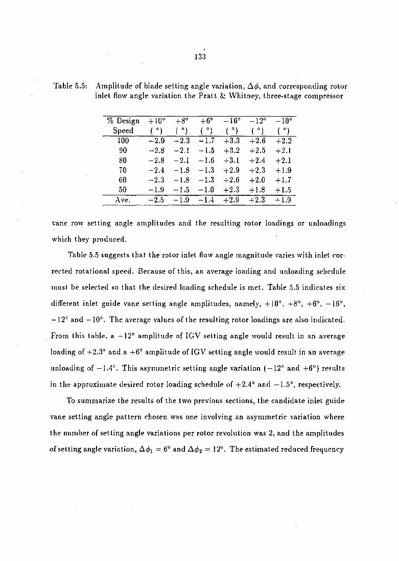
133

Table 5.5: Amplitude of blade setting angle variation, and corresponding rotor inlet flow angle variation the Pratt & Whitney, three-stage compressor

% Design + 10° +8° +6° -16° -12° -10° Speed ( ( °) ( ( °) ( °) ( °)

100 -2.9 -2.3 -1.7 +3.3 +2.6 +2.2 90 -2.8 — 2.1 -1.5 +3.2 +2.5 +2.1 80 -2.8 -2.1 -1.6 +3.1 +2.4 +2.1 70 -2.4 -1.8 —1.3 +2.9 +2.3 + 1.9 60 -2.3 -1.8 -1.3 +2.6 +2.0 + 1.7 50 -1.9 -1.5 -1.0 +2.3 + 1.8 + 1.5

.'Vve. -2.5 -1.9 -1.4 +2.9 +2.3 + 1.9

vane row setting angle amplitudes and the resulting rotor loadings or unloadings

which they produced.

Table 5.5 suggests that the rotor inlet flow angle magnitude varies with inlet cor

rected rotational speed. Because of this, an average loading and unloading schedule

must be selected so that the desired loading schedule is met. Table 5.5 indicates six

different inlet guide vane setting angle amplitudes, namely, +10°, +8°, +6°, -16°,

-12° and -10°. The average values of the resulting rotor loadings are also indicated.

From this table, a -12° amplitude of IGV setting angle would result in an average

loading of +2.3° and a +6° amplitude of IGV setting angle would result in an average

unloading of -1.4°. This asymmetric setting angle variation ( — 12° and +6°) results

in the approximate desired rotor loading schedule of +2.4° and —1.5°, respectively.

To summarize the results of the two previous sections, the candidate inlet guide

vane setting angle pattern chosen was one involving an asymmetric variation where

the number of setting angle variations per rotor revolution was 2, and the amplitudes

of setting angle variation, = 6° and A02 — 12°. The estimated reduced frequency

134

for this variation was 0.19 and the estimated rotor inlet flow angle loading was +2.3°

and -1.4°.

135

6. PRATT & WHITNEY RESULTS AND DISCUSSIONS

6.1 Pratt and Whitney Baseline and Modified Compressor Performance

The effect of compressibility on the proposed method for improving the stall

margin of multistage axial-flow compressors was tested with a Pratt & Whitney,

three-stage, intermediate-speed, axial-flow compressor. Overall performance tests

were performed on the baseline compressor configuration as well as one modified

compressor configuration in which an asymmetric variation in stationary blade setting

angle where = 12°, Aoa = 6° and n = 2 cycles per rotor revolution was the

setting angle schedule. Recall that the modified Pratt & Whitney compressor inlet

guide vane setting angle variation was selected from results of beneficial blade setting

angle variations in the low-speed, three-stage compressor. Particular attention was

focused on the reduced frequency at stall, K,taiti And the resulting rotor inlet flow

angle variation. In this case, the estimated reduced frequency at stall, I\,taih was 0.19

and the rotor inlet flow angle variation maximum and minimum values were -f2.3°

and -1.4°.

The overall performance parameters for the Pratt & Whitney compressor were

corrected mass flow, total-pressure ratio and inlet corrected rotational speed and

are given by Equations (4.10), (4.11) and (4.12). The performance tests involved

identifying the overall performance characteristics of the compressor at six different

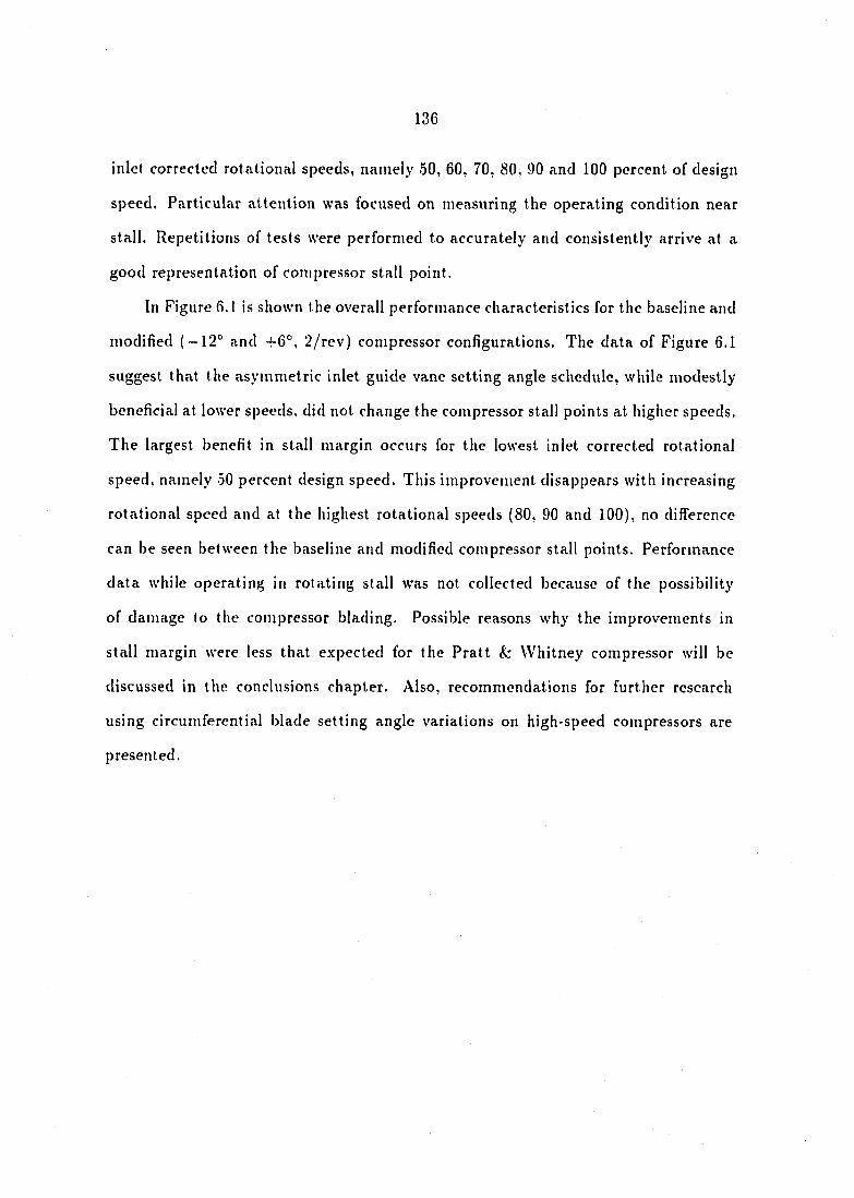
136

inlet corrected rotational speeds, namely 50, 60, 70, 80, 90 and 100 percent of design

speed. Particular attention was focused on measuring the operating condition near

stall. Repetitions of tests were performed to accurately and consistently arrive at a

good representation of compressor stall point.

In Figure 6.1 is shown the overall performance characteristics for the baseline and

modified (-12° and -f6°, 2/rev) compressor configurations. The data of Figure 6.1

suggest that the asymmetric inlet guide vane setting angle schedule, while modestly

beneficial at lower speeds, did not change the compressor stall points at higher speeds,

The largest benefit in stall margin occurs for the lowest inlet corrected rotational

speed, namely 50 percent design speed. This improvement disappears with increasing

rotational speed and at the highest rotational speeds (80, 90 and 100), no difference

can be seen between the baseline and modified compressor stall points. Performance

data while operating in rotating stall was not collected because of the possibility

of damage to the compressor blading. Possible reasons why the improvements in

stall margin were less that expected for the Pratt & Whitney compressor will be

discussed in the conclusions chapter. Also, recommendations for further research

using circumferential blade setting angle variations on high-speed compressors are

presented.

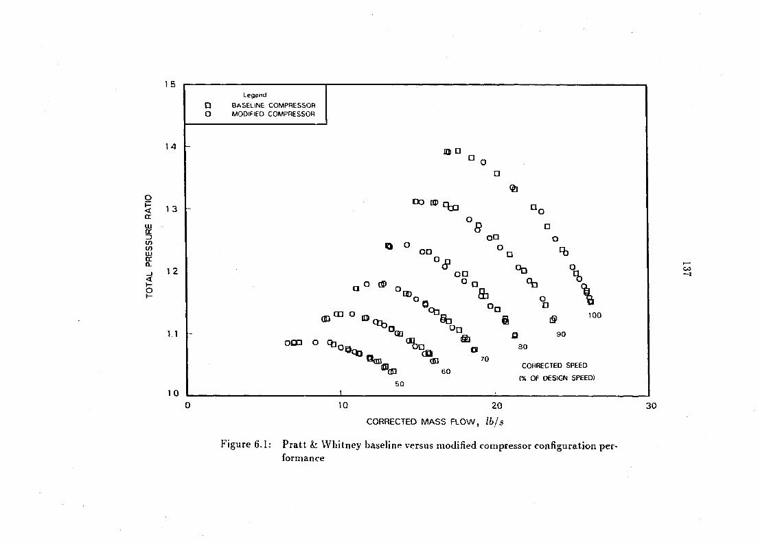
1 5 Legend

D BASELINE COMPRESSOR O MODIFIED COMPRESSOR

1 4 O •

< 1 3 tr

5 U) g D.

1 2

11

1 0

• <a

no CP Re

8 Q O

oo

on o

°(!F %

GO Od

a° ® o

0 &

% %

(g ° ID Cb

%

G Oo •

-"m oq

ë £§» 100

"(ni_ on

90

80

70 % on 60

50

CORRECTED SPEED

(% OF DESIGN SPEED)

10 20

CORRECTED MASS FLOW, lb / s

Figure 6.1: Pratt & Whitney baseline versus modified compressor configuration performance

30

138

6.1.1 Pratt & Whitney detailed flow measurements

In addition to overall performance data collected on the Pratt & Whitney,

intermediate-speed, three-stage, axial-flow compressor, some detailed measurements

of the flow at the inlet and exit of the compressor were performed. Detailed mea

surements were performed for both the baseline compressor as well as the modified

compressor in which the inlet guide vanes were set in an asymmetric variation with

A6i = 12° and Aoo = 6" and K,taii = 0.19. Each compressor configuration was in

strumented with total-pressure probe rakes at four circumferential locations around

the compressor annulus upstream of the inlet guide vanes and downstream of the

compressor exit at the flow measurement section.

These total-pressure and total-temperature measurements were collected at the

six different percent inlet corrected rotational speeds of 50, 60, 70, 80, 90 and 100. For

each of the different speeds, data were collected at an operating condition very near

the actual stall point and at an operating condition closer to design conditions on the

compressor characteristic. In Figures 6.2 and 6.3 are shown the detailed measurement

operating conditions for the baseline compressor and modified compressor configura

tions, respectively. The velocity distributions were determined with Equations (4.2)

through (4.6) discussed in Chapter 4.

In Figures 6.4 through 6.9 are shown the velocity profiles for the baseline com

pressor inlet flow for the six different inlet corrected rotational speeds, namely, 50,

60, 70, 80, 90 and 100, respectively. The figures show the velocity profiles near stall

and at an operating point further along the operating line. The four different circum

ferential locations surveyed are shown in the figures by different dashed lines and are

indicated in the legend. These data suggest that the inlet flow for the baseline com-

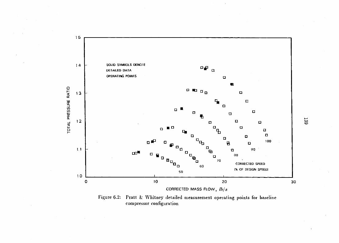
SOLID SYMBOLS DEN01E Of

DETAILED DATA •

OPERATING POINTS p

m

° "O O O O

% • ° • • °

fb o ° •

° q. \ ° °

° a ° °

QiP a g a D

• CORRECTED SPEED • 60

(% OF DESIGN SPEED) 60

I 1

10 20 30

CORRECTED MASS FLOW, lb / s

Figure 6.2: Pratt & Whitney detailed measurement operating points for baseline compressor configuration

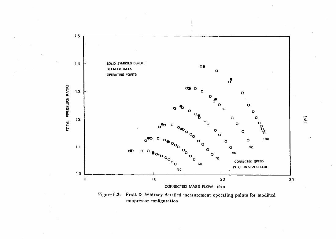
1 5

14

< 13 oc OJ

DC =) to to

a. 12

O h-

1 1

1 0

SOLID SYMBOLS DENOTE

DETAILED DATA

OPERATING POINTS

° o.

o#

# o OB O

O O

D O O °o O O

.#o O °o o

° o, O- o

° O %

o 100

CJD o o o „ O 90

°0 60 CORRECTED SPEED (% OF DESIGN SPEED»

10 20

CORRECTED MASS FLOW, Ib /s

Figure 6.3; Pratt & Whitney detailed measurement operating points for modified compressor configuration

4^ O

30

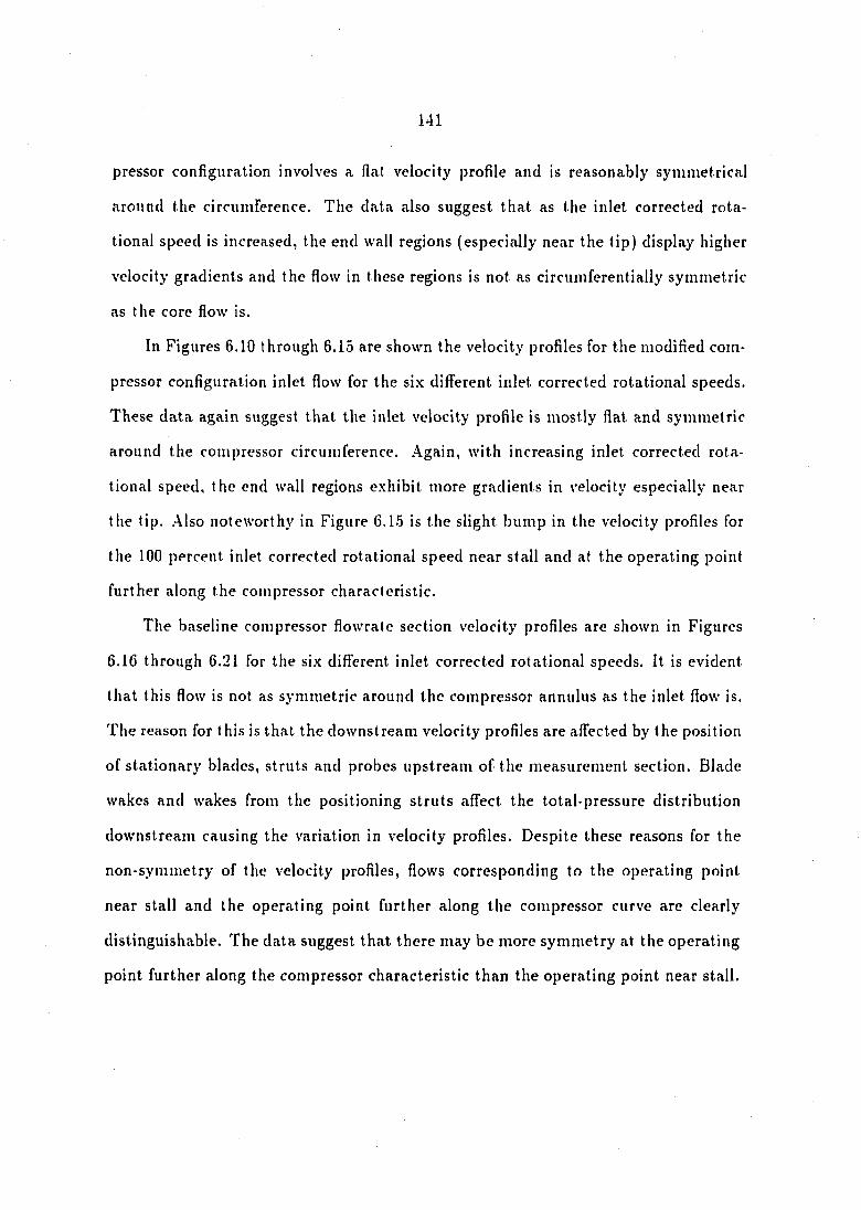
141

pressor configuration involves a flat velocity profile and is reasonably symmetrical

around the circumference. The data also suggest that as the inlet corrected rota

tional speed is increased, the end wall regions (especially near the tip) display higher

velocity gradients and the flow in these regions is not as circuniferentially symmetric

as the core flow is.

In Figures 6.10 through 6.15 are shown the velocity profiles for the modified com

pressor configuration inlet flow for the six diff"erent inlet corrected rotational speeds.

These data again suggest that the inlet velocity profile is mostly flat and symmetric

around the compressor circumference. .4gain, with increasing inlet corrected rota

tional speed, the end wall regions exhibit more gradients in velocity especially near

the tip. .Also noteworthy in Figure 6.1.5 is the slight bump in the velocity profiles for

the 100 percent inlet corrected rotational speed near stall and at the operating point

further along the compressor characteristic.

The baseline compressor flowrate section velocity profiles are shown in Figures

6.16 through 6.21 for the six different inlet corrected rotational speeds. It is evident

that this flow is not as symmetric around the compressor annulus as the inlet flow is.

The reason for this is that the downstream velocity profiles are afl'ected by the position

of stationary blades, struts and probes upstream of the measurement section. Blade

wakes and wakes from the positioning struts afl'ect the total pressure distribution

downstream causing the variation in velocity profiles. Despite these reasons for the

non-symmetry of the velocity profiles, flows corresponding to the operating point

near stall and the operating point further along the compressor curve are clearly

distinguishable. The data suggest that there may be more symmetry at the operating

point further along the compressor characteristic than the operating point near stall.

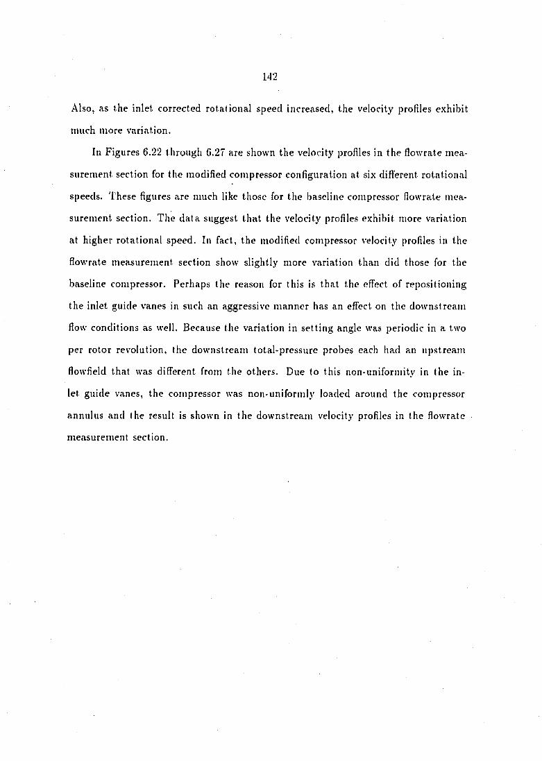
142

Also, as the inlet corrected rotational speed increased, the velocity profiles exhibit

much more variation.

In Figures 6.22 through 6.27 are shown the velocity profiles in the flowrate mea

surement section for the modified compressor configuration at six different rotational

speeds. These figures are much like those for the baseline compressor llowrate mea

surement section. The data suggest that the velocity profiles exhibit more variation

at higher rotational speed. In fact, the modified compressor velocity profiles in the

flowrate measurement section show slightly more variation than did those for the

baseline compressor. Perhaps the reason for this is that the effect of repositioning

the inlet guide vanes in such an aggressive manner has an effect on the downstream

flow conditions as well. Because the variation in setting angle was periodic in a two

per rotor revolution, the downstream total-pressure probes each had an upstream

flowfield that was different from the others. Due to this non-uniformity in the in

let guide vanes, the compressor was non-uniformly loaded around the compressor

annulus and the result is shown in the downstream velocity profiles in the flowrate

measurement section.

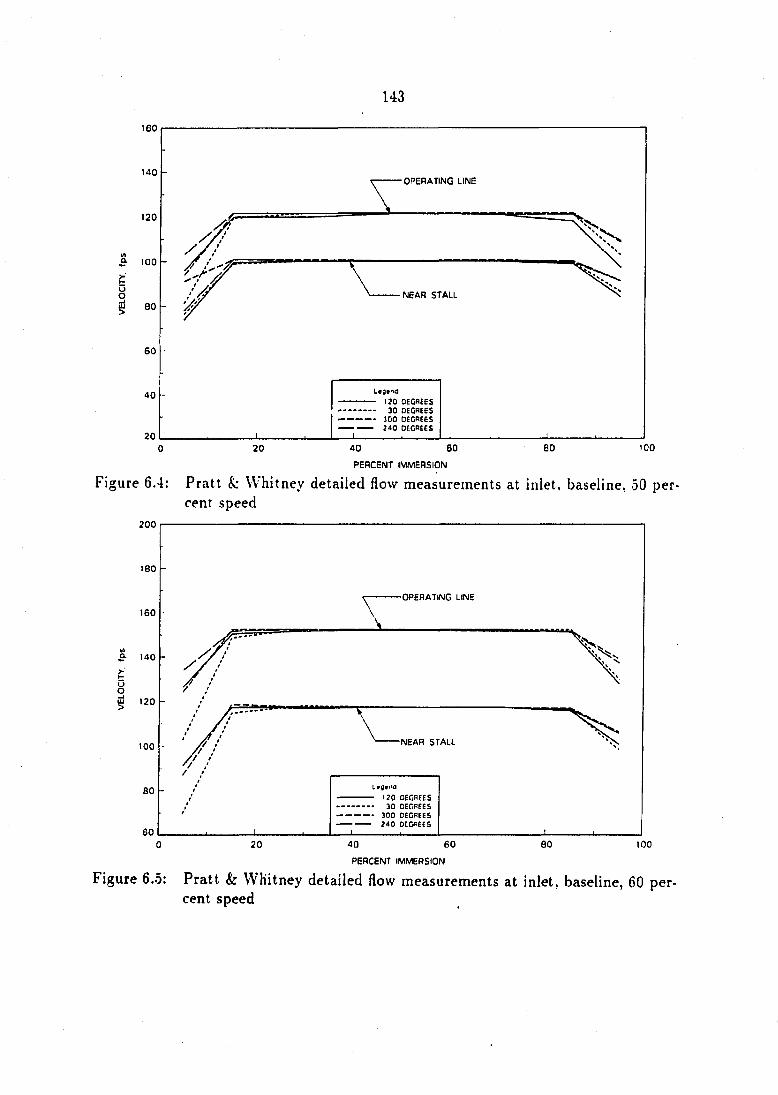
143

160

140

120

3 100

w BO

60

40

20 I

OPERATING LINE

NEAR STALL

Legend

— 120 DEGAGES

-- 30 DEGREES -• 300 DEGREES

- 240 DEGREES

20 80 too 40 60

PERCENT IMMERSION

Figure 6.4: Pratt & Whitney detailed flow measurements at inlet, baseline, 50 percent speed

200

180

160

a. 140 -

O 120 -

100

80 -

OPERATING LINE

NEAR STALL

60

/ leoena

/ 120 DECREES / DEGREES

DEGREES

1 - — 240 DEGREES

20 80 100 40 60

PERCENT IMMERSION


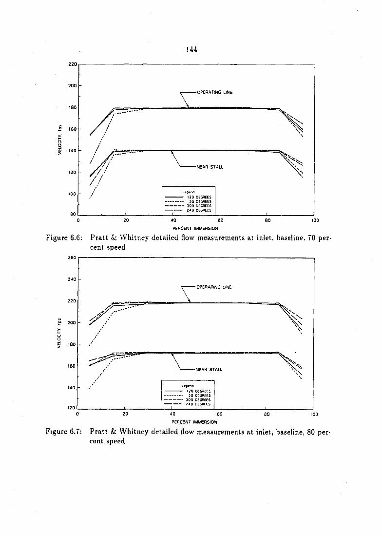
144

220

200 OPERATING LINE

180

_Q. 160

y 140

NEAR STALL 120

- 120 DEGREES • 30 DEGREES

• 300 DEGREES ' 2-ta DECREES

100

60 20 40 0 80 100 PERCENT IMMERSION

Figure 6.6: Pratt & Whitney detailed flow measurements at inlet, baseline. 70 percent speed

260

240

OPERATING LINE

220

200

180

160 NEAR STALL

140

120

0 20 40 60 80 100

PERCENT IMMERSION


145

280

260

240

S- 220

È y g 200

180

160

140

OPERATING LINE

-NEAR STALL

- 120 DEGREES

•• 30 OEOHEES -- 300 DEGREES - 2«0 DEGREES

20 80 100 40 60

PERCENT IMMERSION

Figure 6.8; Pratt & Whitney detailed flow measurements at inlet, baseline. 90 percent speed

300

280

260

S- 240

O 220

200

ISO

160

^ OPERATING LINE

-NEAR STALL

— 120 DEGREES

-- 30 DEGREES

-- 300 DEGREES - 240 DEGREES

20 80 100 40 60

PERCENT IMMERSION


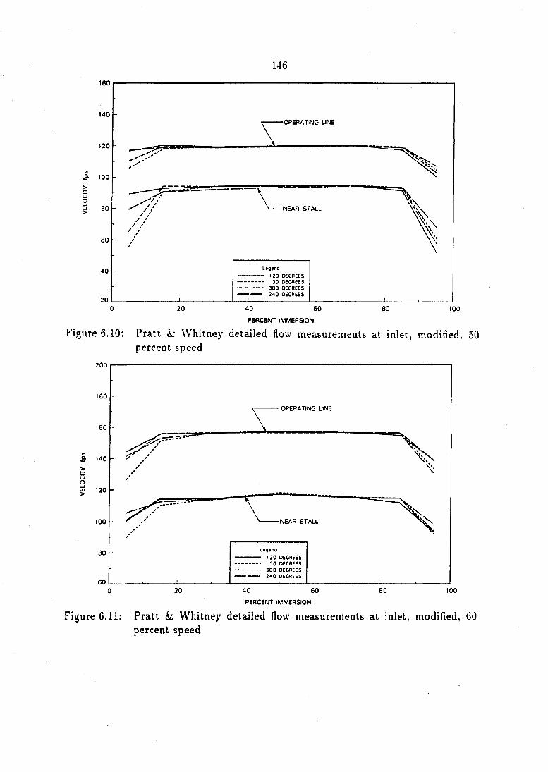
146

160

MO •OPERATING LINE

120

100

80 NEAR STALL

60

Legend

- 1:0 DEGPEES - 30 DEGREES

• 300 DECREES • 240 DEGREES

40

20 0 20 40 60 80 100

PERCENT IMMERSION

Figure 6.10: Pratt & Whitney detailed flow measurements at inlet, modified. 50 percent speed

200

180 OPERATING LINE

160

140

120

NEAR STALL 100

- I JO DEGREES

• 30 DECREES

- 300 DECREES ' Z40 DECREES

60 0 20 40 60 80 100

PERCENT IMMERSION

Figure 6.11: Pratt Whitney detailed flow measurements at inlet, modified, 60 percent speed

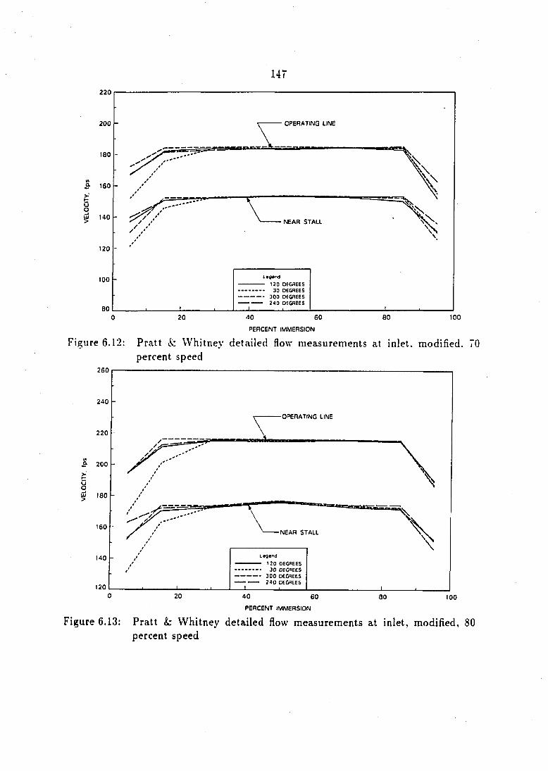
147

220

OPERATING LINE 200

1B0

160

140 NEAR STALL

120

- 130 DEGREES

• 30 DEGREES

• 300 DEGREES • 240 DEGREES

100

0 20 40 60 80 100

PERCENT IMMERSION

Figure 6.12: Pratt & Whitney detailed flow measurements at inlet, modified. 70 percent speed

260

240

OPERATING LINE

220

£• 200

g %

60 NEAR STALL

140

120


Figure 6.13: Pratt & Whitney detailed flow measurements at inlet, modified, 80 percent speed

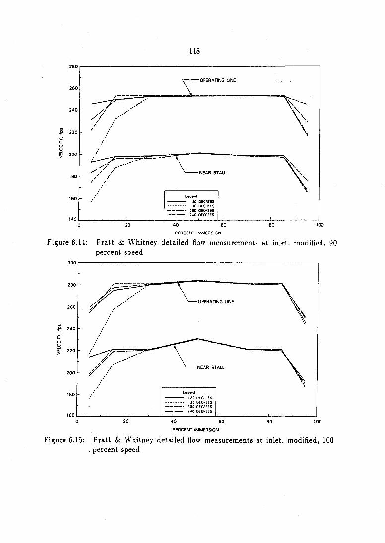
148

260

260

240

a- 220

0 200

ISO

160

140

•OPERATING LINE

-NEAR STALL

J_

— 120 DECREES

-• 30 DEGREES

300 DECREES - }40 DEGREES

20 40 60

PERCENT IMMERSION

80 100

igure 6.14: Pratt & Whitney detailed flow measurements at inlet, modified. 90 percent speed

300

280

260

£• 240

g 220

200

180

160

OPERATING LINE

NEAR STALL

- 120 OEOflEES

•• 30 DEGREES

-- 300 DEGREES - 240 DEGREES

20 80 100

gure 6.15:

40 60

PERCENT IMMERSION

Pratt & Whitney detailed flow measurements at inlet, modified, 100 percent speed

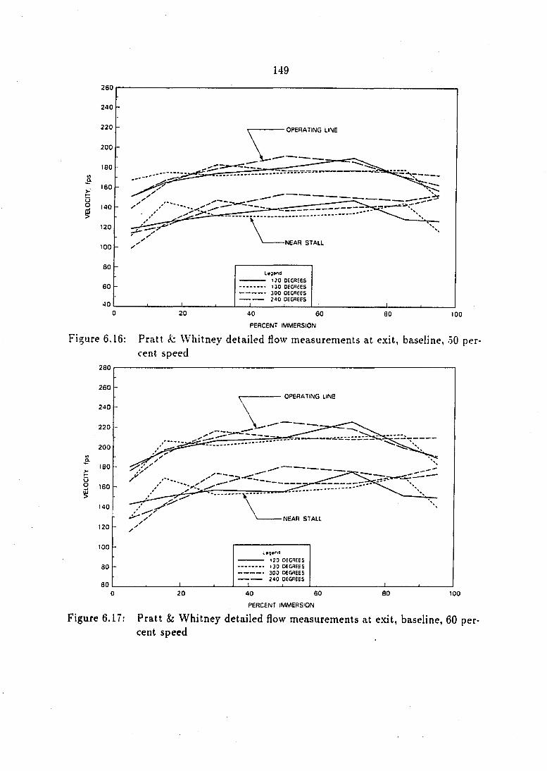
149

u

260

240

220

200

180

160

9 NO

120

100

80

60

40

OPERATING LINE

NEAR STALL

— 120 DECREES

-- 130 DECHEES

-• 300 OEOnEES

- 240 DEGREES

20 80 100 40 60

PERCENT IMMERSION

Figure 6.16: Pratt & Whitney detailed flow measurements at exit, baseline, 50 percent speed

280

260

240

220

200

a 180

M u o 160

140

120

100

80

fiO

OPERATING LINE

NEAR STALL

— 120 DEGREES

-• 130 DEGREES

-• 300 DECREES - 2<10 DEGREES

20 80 100 40 60

PERCENT IMMERSION


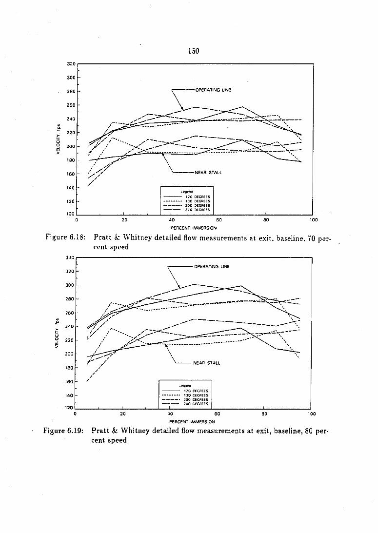
150

320

300

OPERATING LINE 280

260

240

a. 220

>

^ 200

180

NEAR STALL 160

140

- 120 DEGREES

- 130 DEGBEES

• 300 DEGdEES

• 2tO DEGREES

120

100 60 80 100 0 20 40

PERCENT IMMERSION

Figure 6.18: Pratt & Whitney detailed flow measurements at exit, baseline. 70 percent speed

OPERATING LINE 320

300

280

260

240

u P 220

200

NEAR STALL 180

160 Legend - 120 DEGBEES

• 130 DEGHEES

• 300 DEGREES ' 240 DEGREES

140

120



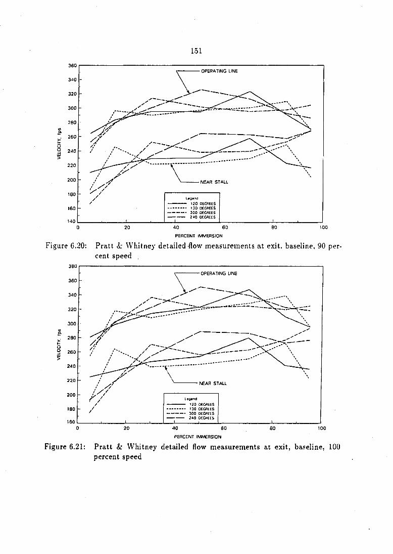
151

360 OPERATING LINE

340

320

300

280

260

Q 240

220

200 NEAR STALL

180 Legend

- 120 DECREES - 130 DEGREES

• 3Q0 DEGREES

- 240 DEGREES

160

140 60 90 20 40 100 0

PERCENT IMMERSION

Figure 6.20: Pratt & Whitney detailed-flow measurements at exit, baseline, 90 percent speed

380

OPERATING LINE

360

340

320

300

G.

280

2 260

240

220 NEAR STALL

// 200

- 120 DEGREES - 130 DECHEES - 300 OEOREES • J40 DEGREES

180

160 0 20 40 60 80 100

PERCENT IMMERSION


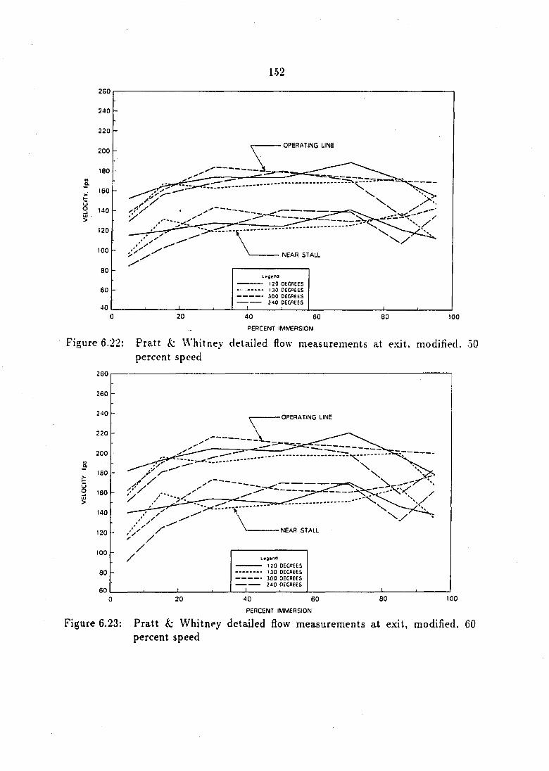
152

260

240

220

OPERATING LINE 200

180

160

140

120

100 NEAR STALL

80 - 120 DECREES • 130 CECflEES

- 300 DECREES

• 240 DECREES 40

0 20 40 60 80 100

PERCENT IMMERSION

Figure 6.22: Pratt &: Whitney detailed flow measurements at exit, modified. 50 percent speed

280

260

240 OPERATING LINE

220

200

160

160

140

NEAR STALL 120

100

- no DEGOEES

- 130 DEGREES . 300 DEGREES

• 240 DEGREES

60 0 20 40 60 80 100

PERCENT IMMERSION

Figure 6.23: Pratt & Whitney detailed flow measurements at exit, modified, 60 percent speed

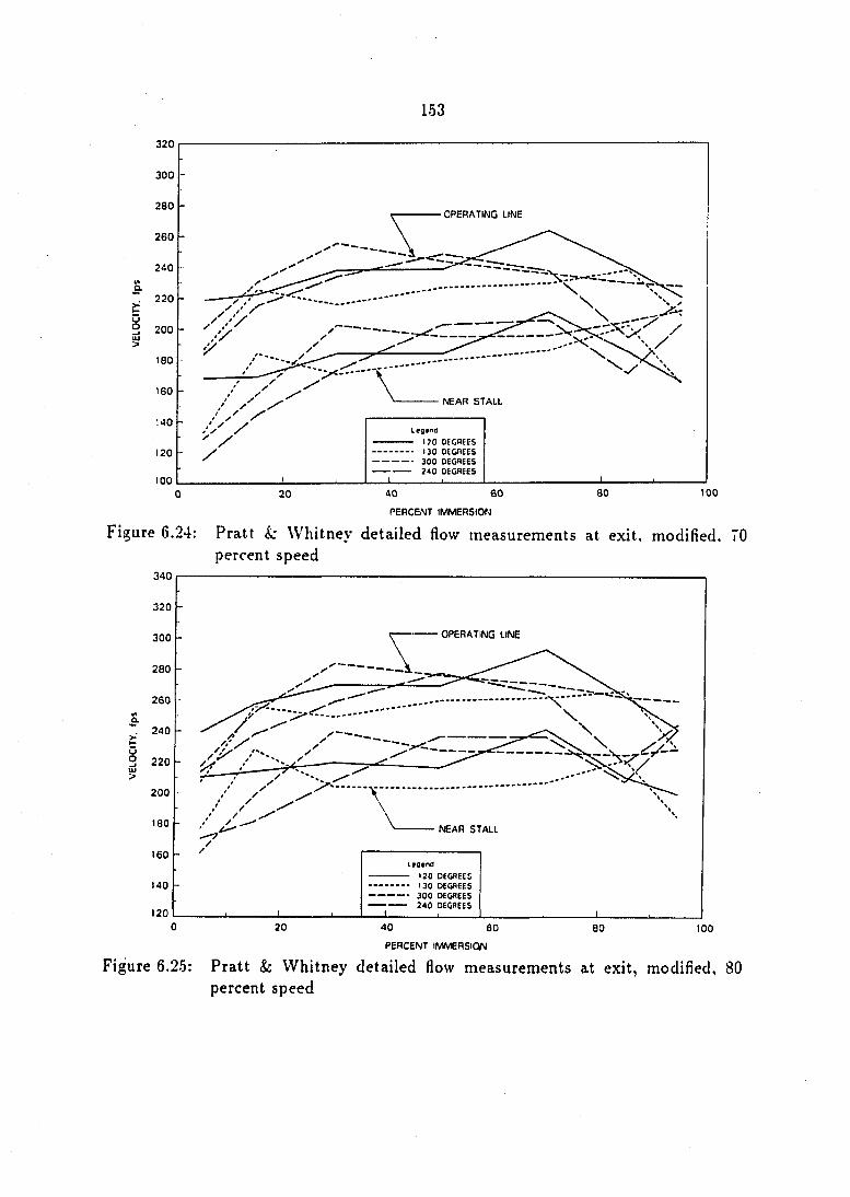
153

320

300

280 OPERATING LINE

260

240

a 220

y P 200

180

160 NEAR STALL

40

- 120 DEGREES

- 130 DEGREES

- 300 DEGREES • 240 decrees

120

100 SO 100 60 40 0 20

PERCENT IMMERSION

Figure 6.24: Pratt & Whitney detailed flow measurements at exit, modified, percent speed

340

320

OPERATING LINE 300

280

260

240

9 220

200

180 NEAR STALL

160 Lfgtnd

- 120 DEGflEES

- 130 DEGREES

• 300 DEGREES

• 240 DEGREES

140

120 0 20 40 60 80 100

PERCENT IMMERSION

Figure 6.25: Pratt Sc Whitney detailed flow measurements at exit, modified, percent speed

154

360

340 OPERATING LINE

320

300

280 a

260

240

220

200 NEAR STALL

180 - 120 OCGBEES

- 130 DE.^EES

- 300 DECREES ' 240 DECREES

160

140 100 60 80 40 20 0

PERCENT IMMERSION


380

360 OPERATING LINE

340

320

300

a. 280

>

§ 260

240

220

200

- 120 DECnEES • no DECREES

• 300 DECREES

' 240 DECREES

NEAR STALL

180

160 0 20 40 60 80 100

PERCENT IMMERSION


7. CONCLUSIONS

The results of the Pratt & Whitney compressor tests suggested that the stall

margin, while only modestly increased at lower rotational speeds, did not improve

at higher speeds. This result leads to the conclusion that although the proposed

method for improving the stall margin worked modestly but consistently in a low-

speed compressor, it did not significantly alter the stalling performance of the Pratt

& Whitney compressor for all speeds tested. One important consolation, however, is

that the aggressive approach used to increase the rotor loading (or diffusion) did not

result in any significant stall margin degradation. Because only one inlet guide vane

setting angle variation was evaluated for the intermediate speed compressor in the

course of this dissertation, a logical recommendation would be to evaluate additional

setting angle variations. Having data for different amplitudes and frequencies of blade

setting angle variations would further explore the possibility of the proposed method

for improving the stall margin of compressors. Some other recommendations include

acquiring detailed data for flow behind the inlet guide vanes as well as behind other

stages. Some in-stall performance data may indicate some interesting observations

as well.

Possible reasons why the stall margin of the higher-speed multistage compressor

was not significantly improved at higher speeds may be linked to the influence of

156

three-dimensional flow and wake interaction effects. Also, because the aspect ratios

involved presently are low, end-wall boundary layer, blade wake and tip and hub

clearance effects are considerable. The dynamic stall results used to develop the

present tests were largely for two-dimensional flows and were not encumbered by

many complexities. It may well be that benefits associated with the present method

are limited in low aspect ratio compressors by three-dimensional flow effects.

The approach of using stationary blade setting angle variations to increase the

average loading of a downstream rotor and to increase the operating range of a com

pressor was both aggressive and risky. The object of the compressor designer, how

ever, is to take this kind of risk hoping that it will improve compressor performance.

Recently, much attention has been focused on methods for maximizing work per stage

to reduce the overall weight of the compressor. To accomplish this end, methods for

achieving higher loading levels in multistage compressors were investigated and re

ported on by VVennerstrom [16]. These methods include vortex generators, suction

and blowing, and casing treatment. .411 of these methods are derived from successful

attempts to control the boundary layer on external two-dimensional surfaces such as

aircraft wings. These methods, however, have met with only limited success and the

reasons for this may help explain why the presently proposed method for increasing

the stall margin of a compressor was only partly successful.

First of all, it is important to point out the trends associated with reducing

aspect ratio in axial-flow compressor blading as described by VVennerstrom [17]. By

reducing the aspect ratio, which is defined as the ratio of blade height to chord, the

three-dimensionality of the flow increases because of secondary flows and end-wall

boundary-layers being more influential in the flow passage. Wennerstrom [17] defined

157

a low-aspect ratio to be about 2.0 and a high-aspect ratio to be greater than 4.0. The

axial-flow compressors used in the present study have rotor aspect ratios which would

be considered low. This would lead us to conclude that the two-dimensional dynamic

stall results may indeed be diminished in the highly three-dimensional flowfields of the

low aspect ratio compressors tested. Wennerstrom also suggests that low aspect ratio

compressors have high tolerance levels to inlet distortions. This may indicate why

there were not any significant degradations in stall margin noted for the compressors

using circumferential variations in blade setting angle.

In tests performed on a high-throughflow transonic axial-flow compressor (Wen

nerstrom (18]), the use of casing vortex generators was evaluated in terms of com

pressor performance. The casing vortex generators resulted in virtually no benefit

in terms of stall margin improvement despite their aggressive attempt to control the

boundary-layer behavior near the tip. In contrast, tests performed with a supersonic

axial compressor stage (Wennerstrom [19)) to evaluate the effects of boundary-layer

control on flow induced separation, seemed to indicate otherwise. In this case, the

use of casing vortex generators suggested that stall margin was improved slightly. In

fact, a radial survey indicated that improvements occurred over full span and not just

at the tip. This would suggest that the behavior near the end wall may determine

the performance of the entire blade span.

The use of suction and blowing to control boundary layer behavior was sum

marized by Wennerstrom [19j. Tapered holes with specific geometry and orientation

were drilled on the compressor outer casing near the rotor blade row. Results from

these test suggest that suction and blowing have no eflfect on stall margin improve

ment unless stall is initiated near the outer casing, in which case there is some benefit

158

in terms of stall margin. In fact, when the suction or blowing was turned off, larger

stall margins were noticed with distorted inlet How. These results led to the use of

casing treatments for improving the stall margins of axial-flow compressors.

.\ll of these boundary layer control methods seem to indicate some important

points. First, the end wall boundary layers seem to control the performance of the

entire blade row to a certain degree. VVennerstrom [16] suggested that separation,

and subsequent stall in a compressor is almost always initiated in a corner between

an airfoil and endwall. Second, because only limited successes in improving the stall

margins of compressor were accomplished using boundary layer control methods, it

is reasonable to conclude that the proposed method can be expected to have only

little beneficial effect as well.

Inasmuch as the proposed method for improving the stall margin of the com

pressor was only partly successful, its future may be as a component of an active

control method. A number of investigators have successfully completed research pro

grams which show significant improvements in compressor performance with the use

of active control methods. In one experiment performed by Ludwig and Nenni [20],

the active control of rotating stall could be accomplished on a low-speed research

compressor as well as a J-85 engine. The active control was an electrical feed-back

control system which used unsteady pressure signals from sensors mounted strate

gically throughout the machines. For the low-speed compressor tests, the variable

geometry feature was the stagger angle of the stator rows. For the J-85 engine, bleed

doors and flaps on the IGVs were the variable geometry feature. When the pressure

sensor indicated stalling was imminent, the variable geometry feature was adjusted

to avoid stall. In the case of the low-speed compressor tests, the stagger angle was

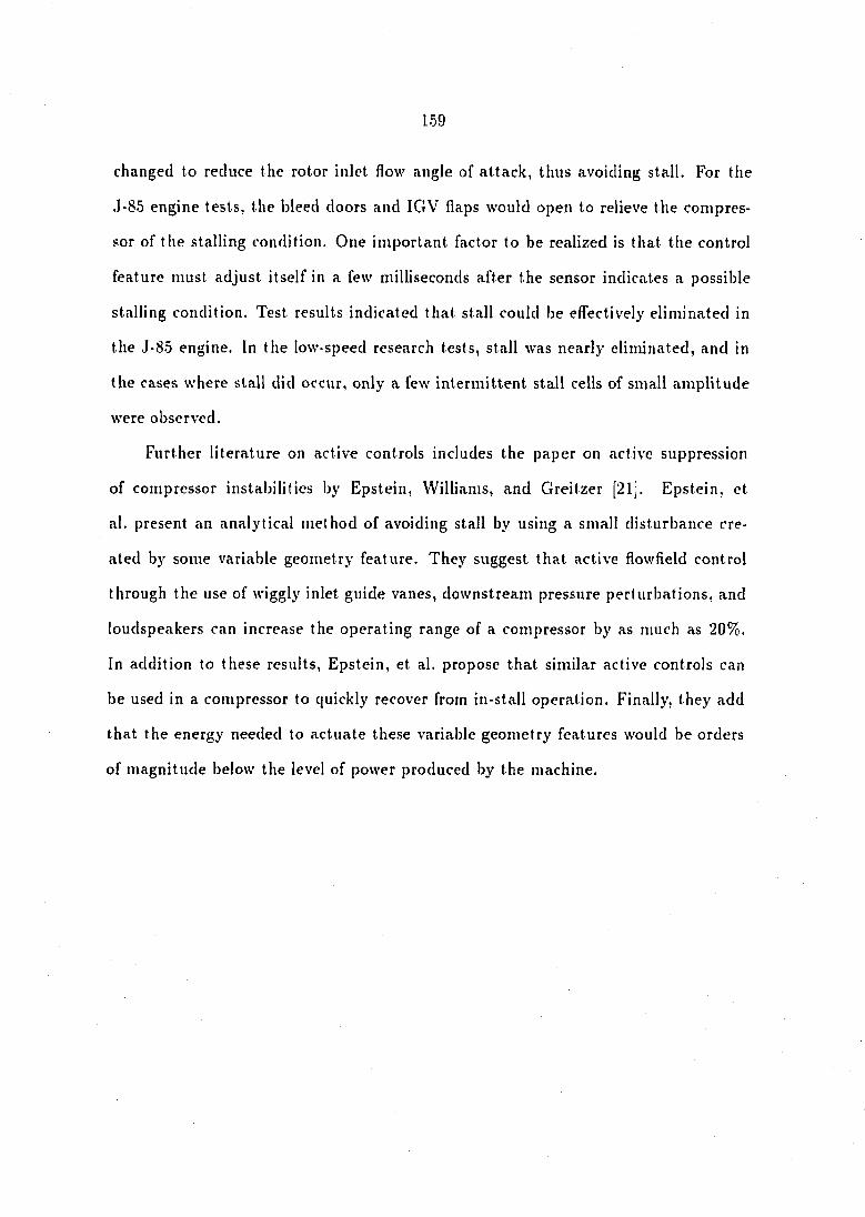
159

changed to reduce the rotor inlet flow angle of attack, thus avoiding stall. For the

J-85 engine tests, the bleed doors and IGV flaps would open to relieve the compres

sor of the stalling condition. One important factor to be realized is that the control

feature must adjust itself in a few milliseconds after the sensor indicates a possible

stalling condition. Test results indicated that stall could be effectively eliminated in

the J-85 engine. In the low-speed research tests, stall was nearly eliminated, and in

the cases where stall did occur, only a few intermittent stall cells of small amplitude

were observed.

Further literature on active controls includes the paper on active suppression

of compressor instabilities by Epstein, Williams, and Greitzer [21). Epstein, et

al. present an analytical method of avoiding stall by using a small disturbance cre

ated by some variable geometry feature. They suggest that active flowfield control

through the use of wiggly inlet guide vanes, downstream pressure perturbations, and

loudspeakers can increase the operating range of a compressor by as much as 20%.

In addition to these results, Epstein, et al. propose that similar active controls can

be used in a compressor to quickly recover from in stall operation. Finally, they add

that the energy needed to actuate these variable geometry features would be orders

of magnitude below the level of power produced by the machine.

160

8. BIBLIOGRAPHY

[1] Copenhaver, VV. W. "Stage Effects on Stalling and Recovery of a High-speed 10-stage Axial-flow Compressor." Ph.D. diss., Iowa State University, 1989.

[2] ".Aerodynamic Design of .\xial-flow Compressors." National Aeronautics and Space .Administration, N.ASA SP-36, 1965.

[3] Greitzer, E. M. "Flow Instabilities in Turbomachines." Lecture Notes from .ASME International Gas Turbine Institute Advanced Course on the Fluid Dynamics of Turbomachinery, July 1986.

[4] Epstein, .A. H. "Smart Engine Components: A Micro in Every Blade?" .Aerospace .America, January 1986.

[•5] McCYoskey, W. J. "Inviscid Flowfield of an Unsteady .Airfoil." AI.AA Journal. Vol. 11. 1973.

[6] Halfman, R. L., Johnson, H. C. and Haley, S. M. "Evaluation of High-Angle-of-.Attack .Aerodynamic-Derivative Data and Stall-Flutter Prediction Techniques." N.AC A TN 2533. November 1951.

[7] McCroskey, VV. J., Carr, L. VV. and McAlister, K, VV. "Dynamic Stall Experiments on Oscillating .Airfoils." AIAA Journal. Vol. 14, 1976.

[8] McCroskey, VV. J. and Pucci, S. L. "Viscous-Inviscid Interaction on Oscillating .Airfoils in Subsonic Flow." .AIAA Journal. Vol. 20, 1982.

[9j Liiva, J. "Unsteady .Aerodynamic and Stall Effects on Helicopter Rotor Blade •Airfoil Sections." Journal of Aircraft. Vol. 6, 1969.

[10] General Electric Instruction Manual. "Model 5GDY34C1 Axial Flow Fan-Dynamometer Set with Speed Variator Power Unit."

[11] Instruction Manual. "Three-stage, Low-speed, Axial-flow Compressor Operation."

161

[12] Rukavina, J. P. "Stall Margin Improvement in Multistage, Axial-flow Compressors by Stationary Blade Setting Angle Modification." M.S. thesis, Iowa State University, 1989.

[13] Thompson, K. E. "The Design and Installation of a Three-stage, Medium Speed, Axial-flow Research Compressor Test Rig." M.S. thesis, Iowa State University, 1987.

[14] Rukavina, .J. P., Okiishi, T. H. and VVennerstrom A. J. "Stall Margin Improvement in Axial-How Compressors by Circumferential Variation of Stationary Blade Setting .Angles." AIAA Paper No. 90-1912, .July 1990.

[1.5] Carter, A. D. S. "The Low Speed Performance of Related Aerofoils in Cascades." Aeronautical Research Council Technical Note, Report No. R. .55, September 1949.

[16] VVennerstrom, J. "Highly Loaded Axial Flow Compressors: History and Current Developments." ASME Journal of Turbomachinery, Vol. 112, October 1990.

[17] VVennerstrom, A. J. "Low Aspect Ratio Axial Flow Compressors: Why and What it Means." ASME .Journal of Turbomachinery, Vol. Ill, October 1989.

[18] VVennerstrom, A. J. "Experimental Study of a High-Through flow Transonic .Axial Compressor Stage." .ASME .Journal of Engineering for Gas Turbines and Power, Vol. 106, July 1984.

[19] VVennerstrom, A. J. "Some Experiments with a Supersonic Axial Compressor Stage." .ASME Journal of Turbomachinery, Vol. 109, July 1987.

[20] Ludwig, G. R. and Nenni, J. P. "A Rotating Stall Control System for Turbojet Engines." .ASME Journal of Engineering for Power, Vol. 101, 1979.

[21] Epstein, A. H., Williams, J. E., and Greitzer, E. M. "Active Suppression of C'ompressor Instabilities." AIA.A Paper No. 86-1994, 1986.

9. ACKNOWLEDGEMENTS

I wish to express my appreciation to my colleagues of the Iowa State University

Engineering Research Institute/Mechanical Engineering Department Turbomachin-

ery Components Research Laboratory for their helpful comments and assistance. I

wish to thank the staff of the Iowa State University Engineering Institute Office of Ed

itorial Services for preparing the figures of this dissertation. Also deep thanks should

go to my major professor and now department chairman, Theodore H. Okiishi, for

his infinite wisdom and guidance. Thanks to my parents Dr. Daniel M. Rukavina and

Patricia A. Rukavina, for spiritual support. Also to my brothers, sisters and extended

family for their support, especially Mara L. Moline, my fiance, for her patience and

continued support throughout this writing. Finally, I am grateful to the U. S. Air

Force for their support of this project through contract F3361.5-87-C-2739 (Project

Engineer: Dr. C. Herbert Law) and to Dr. Arthur J, VVennerstrom of the U. S. Air

Force .Aeropropulsion Laboratory for his helpful suggestions.

163

APPENDIX A: DETAILED FLOW MEASUREMENTS FOR

THREE-STAGE COMPRESSOR

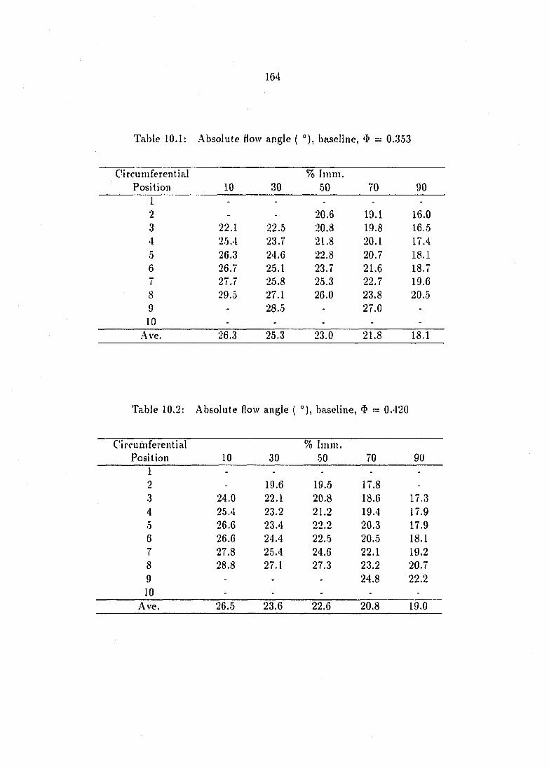
164

Table 10.1: Absolute flow angle ( °), baseline, = 0.353


1 2

- -

20,6 19.1 16.0 3 22.1 22.5 20.8 19.8 16.5 4 25.4 23.7 21.8 20.1 17.4 5 26.3 24.6 22.8 20.7 18.1 6 26.7 25.1 23.7 21.6 18.7 7 27.7 25.8 25.3 22.7 19.6 8 29.5 27.1 26.0 23.8 20.5 9 - 28.0 - 27.0 -

10 - - - - -

Ave. 26.3 25.3 23.0 21.8 18.1

Table 10.2: Absolute flow angle ( °), baseline, $ = 0.420

Circumferential % Imm, Position 10 30 50 70 90

1 2

-

19.6 19,5 17.8 -

3 24.0 22.1 20,8 18.6 17.3 4 25.4 23.2 21.2 19.4 17.9 5 26.6 23.4 22,2 20.3 17.9 6 26.6 24.4 22,5 20.5 18.1 7 27.8 25.4 24.6 22.1 19.2 8 28.8 27.1 27.3 23.2 20.7 9 - - - 24.8 22.2 10 - - - - -

Ave. 26.5 23,6 22.6 20.8 19.0

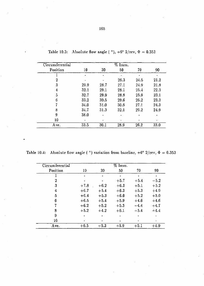
165

Table 10.3: .Absolute flow angle ( °), +6° 2/rev, $ — 0.353

Circumferential % Imm. Position 10 30 50 7^ 90_

2 - - 26.3 24.5 21.2 3 29.9 28.7 27.1 24.9 21.8 4 32.1 29.1 28.1 25.4 22.3 5 32.7 29.9 28.8 25.9 23.1 6 33.2 30.5 29.6 26.2 23.3 7 .34.0 31.0 30.6 27.1 24.3 8 .34.7 31.3 32.1 29.2 24.9 9 38.0

10

Aw. 3^ 3CLI 2Ô 261 ^

Table 10.4: .Absolute flow angle { °) variation from baseline, +6° 2/rev, = 0.353

Circumferential % Imm. Position 10 30 50 70 ^

2 - - +5.7 +5.4 +5.2 3 +7.8 +6.2 +6.3 +5.1 +5.2 4 +6.7 +.5.4 +6.3 +5.3 +4.9 5 +6.4 +5.3 +6.0 +5.2 +5.0 6 +6.5 +5.4 +5.9 +4.6 +4.6 7 +6.2 +5.2 +5.3 +4.4 +4.7 8 +5.2 +4.2 +6.1 +5.4 +4.4 9 . . . . .

1 0 . . . . .

Ave. +6.5 +5.3 +5.9 +5.1 +4.9

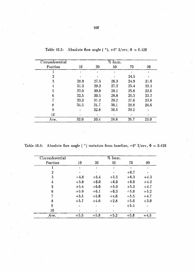
166

Table 10.5: Absolute flow angle ( °), +6° 2/rev, <5 = 0.420


1 2

• " -

24.5 -

3 28.8 27.5 26.3 24.9 21.6 4 31.2 29.2 27.2 25.4 22.1 5 32.0 30.0 28.1 25.6 22.6 6 32.5 30.5 28.8 26.3 23.3 7 33.3 31.2 29.2 27.6 23.9 8 34.5 31.7 30.1 28.8 24.6 9 - 32.8 30.5 30.2 -

10 - ' - - -

Ave. 32.0 30.4 28.6 26.7 23.0

Table 10.6: Absolute flow angle ( °) variation from baseline, +6° 2/rev, «D = 0.420


1 2

- - -

+6.7 -

3 +4.8 +5.4 +5.5 +6.3 +4.3 4 +5.8 +6.0 +6.0 +6.0 +4.2 5 +5.4 +6.6 +5.9 +5.3 +4.7 6 +5.9 +6.1 +6.3 +5.8 +5.2 7 +5.5 +5.8 +4.6 +5.5 +4.7 8 +5.7 +4.6 +2.8 +5.6 +3.9 9 - - - +5.4 -

10 - - - - -

Ave. 4*5.5 +5.8 +5.2 +5.8 +4.5

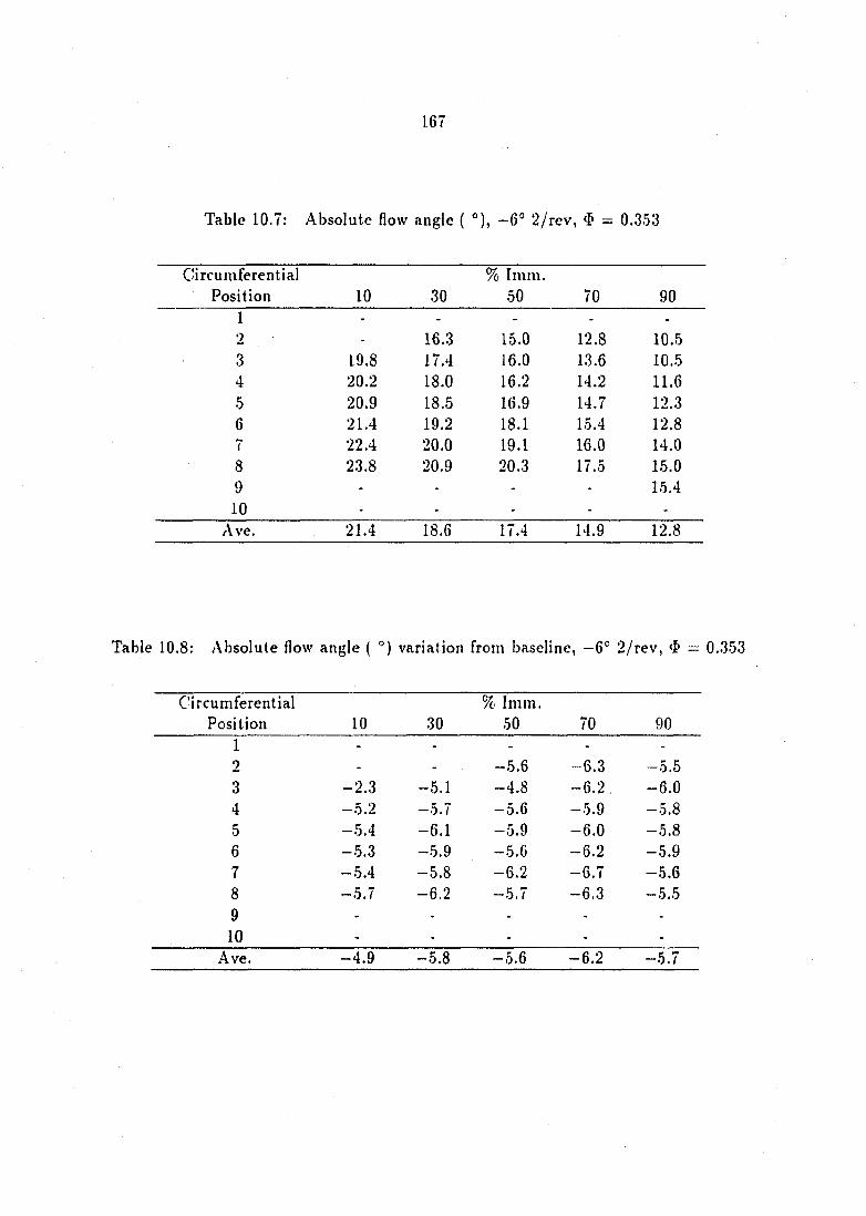
167

Table 10.7: Absolute flow angle ( °), —6° 2/rev, $ — 0.353


1 2

-

16.3 15.0 12.8 10.5 3 19.8 17.4 16.0 13.6 10.5 4 20.2 18.0 16.2 14.2 11.6 5 20.9 18.5 16.9 14.7 12.3 6 21.4 19.2 18.1 15.4 12.8 7 22.4 20.0 19.1 16.0 14.0 8 23.8 20.9 20.3 17.5 15.0 9 - - - - 15.4

10 - - - - -

Ave. 21.4 18.6 17.4 14.9 12.8

Table 10.8: .Absolute flow angle ( °) variation from baseline, —6° 2/rev, = 0.353

Circumferential Position 10 30

% Imm. 50 70 90

1 2 3 4 5 6 7 8 9

10

-2.3 -5.2 -5.4 -5.3 -5.4 -5.7

-5.1 -5.7 -6.1 -5.9 —5.8 -6.2

-5.6 —4.8 -5.6 -5.9 -5.6 -6.2 -5.7

-6.3 -6.2 -5.9 -6.0 -6.2 -6.7 -6.3

-5.5 -6.0 -5.8 -5.8 -5.9 —5.6 —5.5

Ave. -4.9 —5.8 —5.6 -6,2 -5.7

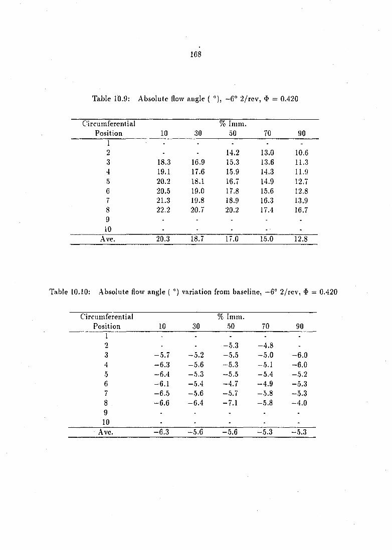
168

Table 10.9: Absolute flow angle ( "), -6° 2/rev, $ = 0.420


1 - - - - -

2 - - 14.2 13.0 10.6 3 18.3 16.9 15.3 13.6 11.3 4 19.1 17.6 15.9 14.3 11.9 5 20.2 18.1 16.7 14.9 12.7 6 20.5 19.0 17.8 15.6 12.8 7 21.3 19.8 18.9 16.3 13.9 8 22.2 20.7 20.2 17.4 16.7 9 - - - - -

10 - - - -

Ave. 20.3 18.7 17.0 15.0 12.8

Table 10.10: .Absolute flow angle ( °) variation from baseline, —6° 2/rev, <I> = 0.420


% Inim. 50 70 90

1 2 3 4 5 6 7 8 9 10

-5.7 -6.3 -6.4 -6.1 -6.5 -6.6

-5.2 -5.6 -5.3 -5.4 -5.6 -6.4

-5.3 -5.5 -5.3 -5.5 -4.7 -5.7 -7.1

-4.8 -5.0 -5.1 -5.4 -4.9 -5.8 -5.8

-6.0 -6.0 -5.2 -5.3 -5.3 -4.0

Ave. -6.3 -5.6 —5.6 —5.3 -5.3

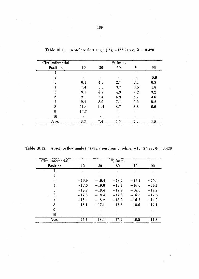
169

Table 10.11: Absolute flow angle ( °), -16" 2/rev, = 0.420


% Imm. 50 70 90

1 2 3 4 5 6 7 8 9

10

6.1 7.4 8.1 9.1 9.4

11.4 13.7

4.3 .5.6 6.7 7.4 8.9 11.4

2.7 3.7 4.9 5.9 7.1 8.7

2.1 3.5 4.2 5.1 6.0 8.8

-0,6 0.9 1.8 3.2 3.6 5.2 6.6

Ave. 9.3 7.4 5.5 5.0 3.0

Table 10.12: Absolute flow angle ( °) variation from baseline, -16° 2/rev, = 0.420


% Imm. 50 70 90

1 2 3 4 5 6 7 8 9

10

-16.0 -18.0 -18.2 -17.6 -18.4 -18.1

-19.4 -19.0 -18.4 -18.4 -18.2 -17.1

—18.1 -18.1 -17.9 -17.8 -18.2 -17.3

-17.7 -16.6 -16.5 -16.5 -16.7 -15.0

-15.4 -16.1 -14.7 -14.5 -14.0 -14.1

1 2 3 4 5 6 7 8 9

10 . . . . .

Ave. -17.7 -18.4 -17.9 -16.5 -14.8

170

Table 10.13: .Absolute flow angle ( °), —16° 2/rev, $ = 0.353


% Imm. 50 70 90

1 2 3 4 5 6 7 8 9

10

5.7 7.6 7.8 8.8 9.8 12.0

1.2 4.0 5.5 6.6 7.7 8.5

10.0

3.0 4.0 5.2 6.9 8.0

10.1

-1.9 1.1 3.1 4.7 5.6 6.9 8.1

-1.1 1.1 2.5 4.0 5.0 7.0 9.1

.•\ve. 8.6 6.2 6.2 3.9 3.9

Table 10.14: Absolute flow angle ( °) variation from baseline, -16° 2/rev, = 0.


1 - - - - -

2 - - - -21.0 -17.1 3 -16.4 -18.5 -17.8 -18.7 -15.4 4 -17.8 -18.2 -17.8 -17.0 -14.9 5 -18.5 -18.0 -17.6 -16.0 -14.1 6 -17.9 -17.4 -16.8 -16.0 -13.7 7 -18.0 -17.3 -17.3 -15.8 -12.6 8 -17.5 -17.1 -15.9 -15.7 -11.4 9 - - - - -

10 - - - • -

Ave. -17.7 -17.8 -17.2 -17.2 -14.2

171

APPENDIX B: VELOCITY DIAGRAM CALCULATIONS FROM

DETAILED MEASUREMENT DATA

172

Table 11.1: Detailed flow measurement data, baseline, 'I' = 0.353

% P,( ,dt V'l V'tf, Ui lUff, Va-, wi KHF Imm. Ib / i i }^ ( °) f t / s f t / s f t / s f t / s f t j s f t / s { ° )

10 -0.0103 18.1 36.60 11.37 94.81 83.44 34.79 90.40 67.4 0.23

30 -0.0105 21.8 .36.92 13.71 88.94 75.23 34.28 82.67 65.5 0.25

50 -0.0107 23.0 37.30 14.57 83.08 68.51 34.33 76.63 63.4 0.27

70 -0.0110 25.3 37.74 16.13 77.21 61.08 34.12 69.96 60.8 0.30

90 -0.0113 26.3 .38.35 16.99 71.35 .54.36 34.38 64.32 57.7 0.32

Table 11.2; Detailed flow measurement data, baseline, ^ = 0.420

% V'l V's, lue^ Ix, ifi !3[ Imm. ( °) f t / s f t j s f t j s f t / s f t / s f t / s ( ° )

10 -0.0156 19.0 45.04 14.66 94.81 80.15 42.59 90.76 62.0

30 -0.0158 20.8 45.35 16.10 88.94 72.84 42.39 84.28 59.8

50 -0.0161 22.6 45.76 17.58 83.08 65.50 42.25 77,94 57.2

70 -0.0165 23.6 46.32 18.54 77.21 .58.67 42.45 72.42 .54.1

90 -0.0170 26.5 46.97 20.96 71.35 .50.39 42.04 65.62 .50.2

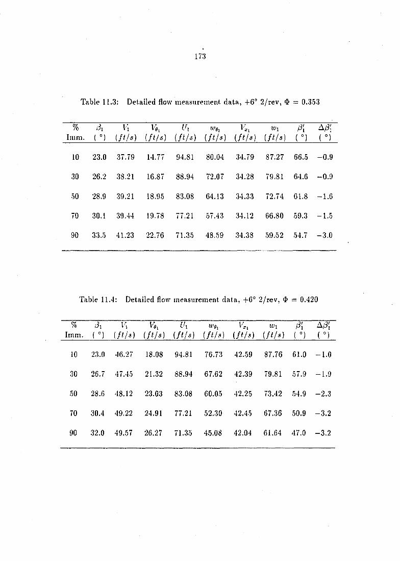
173

Table 11.3: Detailed flow measurement data, +6° 2/rev, $ = 0.353

% Imm. ( 1

Vi (//A)

n'e, (A/^)

W i i f t / s ) ( ° )

<1

10 23.0 37.79 14.77 94.81 80.04 34.79 87.27 66.5 -0.9

30 26.2 38.21 16.87 88.94 72.07 34.28 79.81 64.6 -0.9

50 28.9 39.21 18.95 83.08 64.13 34.33 72.74 61.8 -1.6

70 30.1 39.44 19.78 77.21 .57.43 34.12 66.80 59.3 -1.5

90 33.5 41.23 22.76 71.35 48.59 34.38 59.52 54.7 —•3.0

Table 11.4: Detailed flow measurement data, 4-6° 2/rev, = 0.420

% Imm. ( ° ) (/(//I)

lé, (/</^)

I h (A/;*)

U'g, i f t / s )

V'x. (/(A) (/(A) ( ° ) ( ° )

10 23.0 46.27 18.08 94.81 76.73 42..59 87.76 61.0 -1.0

30 26.7 47.45 21.32 88.94 67.62 42.39 79.81 57.9 -1.9

50 28.6 48.12 23.03 83.08 60.05 42.25 73.42 54.9 -2.3

70 30.4 49.22 24.91 77.21 52.30 42.45 67.36 .50.9 -3.2

90 32.0 49.57 26.27 71.35 45.08 42.04 61.64 47.0 -3.2

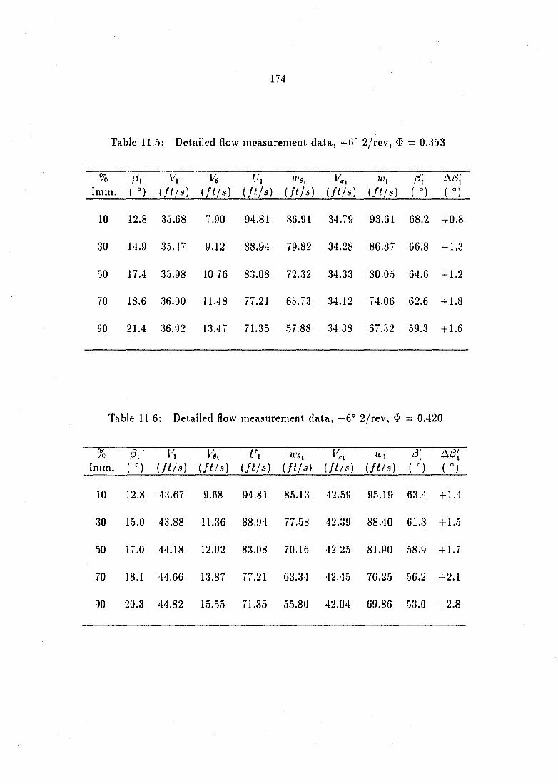
174

Table 11.5: Detailed flow measurement data, —6° 2/rev, $ = 0.353

% I mm. ( " )

I'l i f f / s )

f'l i f t h ) (/(/a)

«'1 i f t / s )

I3[ ( °) ( ° )

10 12.8 35.68 7.90 94.81 86.91 34.79 93.61 68.2 +0.8

30 14.9 35.47 9.12 88.94 79.82 .34.28 86.87 66.8 +1.3

50 17.4 35.98 10.76 83.08 72.32 .34.33 80.05 64.6 + 1.2

70 18.6 36.00 11.48 77.21 65.73 34.12 74.06 62.6 + 1.8

90 21.4 .36.92 13.47 71.35 57.88 34.38 67.32 59.3 + 1.6

Table 11.6: Detailed flow measurement data, —6° 2/rev, = 0.420

% Imm.

/il ( ° )

Vi (/<A) (/</;») (/<//»)

IVs I (/<A)

tt'i i f t i s ) ( 1 ( ° )

10 12.8 43.67 9.68 94.81 85.13 42.59 95.19 63.4 + 1.4

30 15.0 43.88 11.36 88.94 77.58 42.39 88.40 61.3 +1 ..5

50 17.0 44.18 12.92 83.08 70.16 42.25 81.90 58.9 + 1.7

70 18.1 44.66 13.87 77.21 63.34 42.45 76.25 .56.2 +2.1

90 20.3 44.82 15.55 71.35 .55.80 42.04 69.86 53.0 +2.8

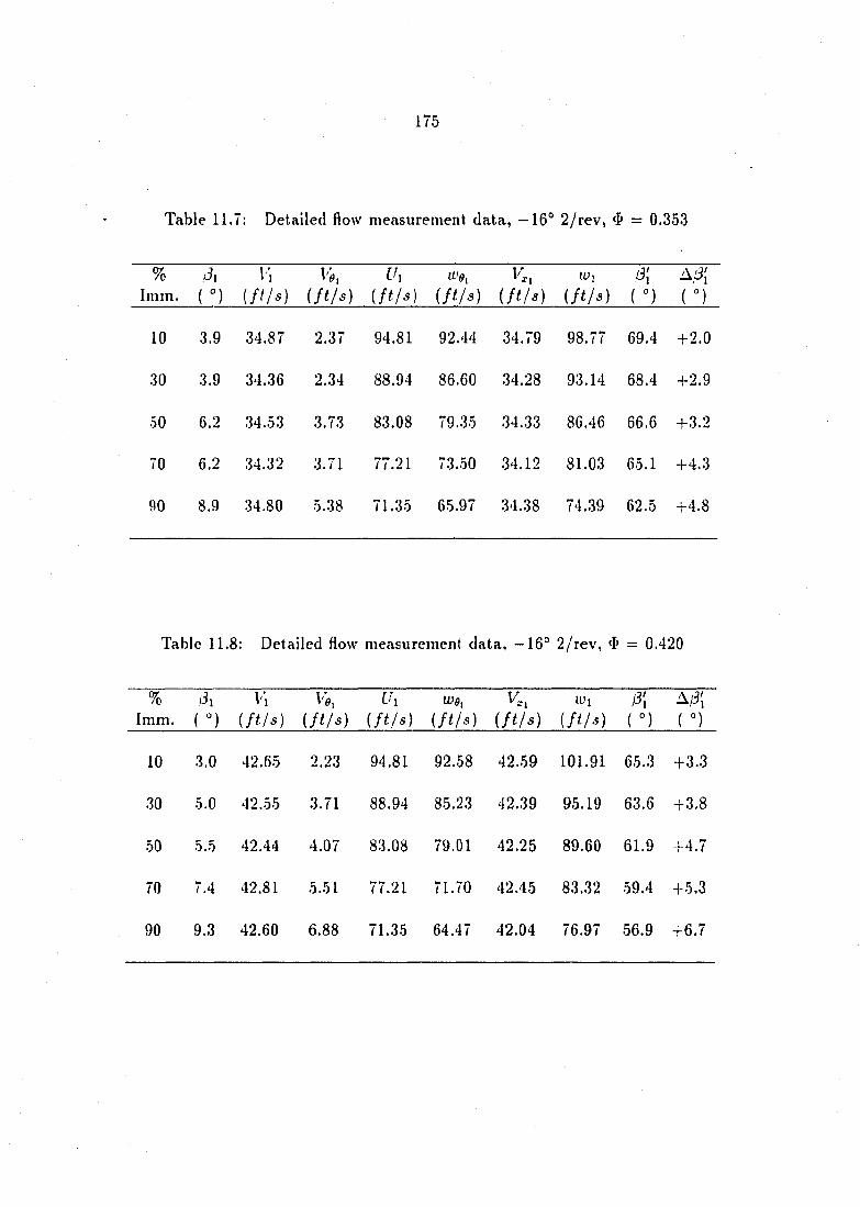
176

Table 11.7: Detailed flow measurement data, —16° 2/rev, = 0.353

% Imm.

.iSi { ° )

li (/</';) i f t / s ) i f t l s ) i f t / s ) i f t / s )

W i i f t l s ) ( °) i " )

10 3.9 34.87 2.37 94.81 92.44 34.79 98.77 69.4 +2.0

30 3.9 34.36 2.34 88.94 86.60 34.28 93.14 68.4 +2.9

50 6.2 .34.53 3.73 83.08 79.35 34.33 86.46 66.6 +3.2

70 6.2 34.32 3.71 77.21 73.50 34.12 81.03 65.1 +4.3

90 8.9 34.80 5.38 71.35 65.97 34.38 74.39 62.5 +4.8

Table 11.8: Detailed flow measurement data, —16° 2/rev, — 0.420

% Imm. (

V'l (/(/a)

Vi, U x (/(A)

Ws, ( f t / ^ ) i f i / s )

W i (/(//») ( ° )

A/3; ( ° )

10 3.0 42.65 2.23 94.81 92.58 42.59 101.91 65.3 +3.3

30 5.0 42.55 3.71 88.94 85.23 42.39 95.19 63.6 +3.8

50 5.5 42.44 4.07 83.08 79.01 42.25 89.60 61.9 +4.7

70 7.4 42.81 5.51 77.21 71.70 42.45 83.32 59.4 +5.3

90 9.3 42.60 6.88 71.35 64.47 42.04 76.97 56.9 +6.7

Modification of axial-flow compressor stall margin by ...

Documents

Transcript of Modification of axial-flow compressor stall margin by ...