
Simulation and Modelling Techniques for Noise in Radio ... · the noise analysis methodology for...
181
Simulation and Modelling Techniques for Noise in Radio Frequency Integrated Circuits by Amit Mehrotra B. Tech. (Indian Institute of Technology, Kanpur) 1994 M. S. (University of California at Berkeley) 1996 A dissertation submitted in partial satisfaction of the requirements for the degree of Doctor of Philosophy in Engineering-Electrical Engineering and Computer Sciences in the GRADUATE DIVISION of the UNIVERSITY of CALIFORNIA at BERKELEY Committee in charge: Professor Alberto L Sangiovanni-Vincentelli, Chair Professor Robert K Brayton Professor J George Shanthikumar Fall 1999
Transcript of Simulation and Modelling Techniques for Noise in Radio ... · the noise analysis methodology for...
Simulation and Modelling Techniques for Noise in Radio FrequencyIntegrated Circuits
by
Amit Mehrotra
B. Tech. (Indian Institute of Technology, Kanpur) 1994M. S. (University of California at Berkeley) 1996
A dissertation submitted in partial satisfaction of the
requirements for the degree of
Doctor of Philosophy
in
Engineering-Electrical Engineering and Computer Sciences
in the
GRADUATE DIVISION
of the
UNIVERSITY of CALIFORNIA at BERKELEY
Committee in charge:
Professor Alberto L Sangiovanni-Vincentelli, ChairProfessor Robert K BraytonProfessor J George Shanthikumar
Fall 1999

The dissertation of Amit Mehrotra is approved:
Chair Date
Date
Date
University of California at Berkeley
1999
Simulation and Modelling Techniques for Noise in Radio Frequency
Integrated Circuits
Copyright 1999
by
Amit Mehrotra
1
Abstract
Simulation and Modelling Techniques for Noise in Radio Frequency Integrated
Circuits
by
Amit Mehrotra
Doctor of Philosophy in Engineering-Electrical Engineering and Computer Sciences
University of California at Berkeley
Professor Alberto L Sangiovanni-Vincentelli, Chair
In high speed communications and signal processing applications, random electri-
cal noise that emanates from devices has a direct impact on critical high level specifications,
for instance, system bit error rate or signal to noise ratio. Hence, predicting noise in RF
systems at the design stage is extremely important. Additionally, with the growing com-
plexity of modern RF systems, a flat transistor-level noise analysis for the entire system
is becoming increasingly difficult. Hence accurate modelling at the component level and
behavioural level simulation techniques are also becoming increasingly important. In this
work, we concentrate on developing noise simulation techniques and mathematically accu-
rate noise models at the component level. These models will also enable behavioural level
noise analysis of large RF systems.
The difference between our approach of performing noise analysis for RF circuits
and the traditional techniques is that we first concentrate on the noise analysis for oscillators
instead of non-oscillatory circuits. As a first step, we develop a new quantitative description
of the dynamics of stable nonlinear oscillators in presence of deterministic perturbations.
Unlike previous such attempts, this description is not limited to two-dimensional system of
equations and does not make any assumptions about the type of nonlinearity. By consider-
ing stochastic perturbations in a stochastic differential calculus setting, we obtain a correct
mathematical characterization of the noisy oscillator output. We show that the oscillator
output is the sum of two stochastic processes: a large signal stochastic process with Brow-
nian motion phase deviation and a small “amplitude” noise process. We further show that
2
the response of the noisy oscillator is asymptotically wide-sense stationary with Lorentzian
power spectral density. We also show that the second order statistics of this output are
characterized by a single scalar constant. We present efficient numerical techniques both
in time domain and in frequency domain for computing this constant. This approach also
determines the relative contribution of the device noise sources to phase noise, which is very
useful for oscillator design.
This new way of characterizing the oscillator output has a far-reaching impact on
the noise analysis methodology for nonautonomous circuits, which we also investigate. We
develop noise analysis techniques for nonautonomous circuits that are driven by a large
single-tone periodic signal with phase noise. We formulate this problem as a stochastic
differential equation and solve it in presence of white noise sources. We show that the
output of a nonlinear nonautonomous circuit, in presence of input signal phase noise which
has Brownian motion phase deviation, is asymptotically stationary. We also show that the
Lorentzian spectrum of the input signal and the characteristics of the Brownian motion
input phase deviation process are preserved at the output. We further show that the input
signal phase noise contributes an additional wide-band amplitude noise term that appears
as a white noise source modulated by the time derivative of the steady state response.
We also extend this analysis to circuits that are driven by more than one large
periodic signal that are corrupted by phase noise. We show that, similar to the one tone
case, the output of a nonautonomous circuit driven by two or more large tones is also
asymptotically stationary. We show that phase noise of each input signal contributes one
additional white noise source that is modulated by derivatives of the steady state response.
These models for autonomous and nonautonomous components of RF circuits will
enable one to perform nonlinear noise simulation at the behavioural level for large RF
systems. These models can also be used for behavioural level performance optimization
and constraint generation for the RF components.
Professor Alberto L Sangiovanni-VincentelliDissertation Committee Chair

iii
To Ma and Pitaji
iv
Contents
List of Figures vii
List of Tables ix
1 Introduction 11.1 Architecture of an RF Front End . . . . . . . . . . . . . . . . . . . . . . . . 21.2 Motivation . . . . . . . . . . . . . . . . . . . . . . . . . . . . . . . . . . . . 6
1.2.1 Noise Sources in RF Transceiver . . . . . . . . . . . . . . . . . . . . 61.2.2 Autonomous versus Nonautonomous Circuits . . . . . . . . . . . . . 8
1.3 Thesis Overview . . . . . . . . . . . . . . . . . . . . . . . . . . . . . . . . . 9
2 Overview of Existing Techniques 112.1 Perturbation Analysis of a Nonoscillatory System . . . . . . . . . . . . . . . 112.2 Noise Analysis of Nonoscillatory Systems . . . . . . . . . . . . . . . . . . . 13
2.2.1 LPTV Approaches and Extensions . . . . . . . . . . . . . . . . . . . 142.2.2 Time Domain Analysis . . . . . . . . . . . . . . . . . . . . . . . . . . 152.2.3 Our Approach . . . . . . . . . . . . . . . . . . . . . . . . . . . . . . 15
2.3 Oscillator Phase Noise Analysis . . . . . . . . . . . . . . . . . . . . . . . . . 162.3.1 LTI/LTV Noise Analysis . . . . . . . . . . . . . . . . . . . . . . . . . 162.3.2 Timing Jitter Analysis . . . . . . . . . . . . . . . . . . . . . . . . . . 172.3.3 Time Domain Noise Analysis . . . . . . . . . . . . . . . . . . . . . . 182.3.4 Other Approaches . . . . . . . . . . . . . . . . . . . . . . . . . . . . 182.3.5 Our Approach . . . . . . . . . . . . . . . . . . . . . . . . . . . . . . 19
3 Perturbation Analysis of Stable Oscillators 203.1 Mathematical Preliminaries . . . . . . . . . . . . . . . . . . . . . . . . . . . 203.2 Perturbation Analysis Using Linearization . . . . . . . . . . . . . . . . . . . 23
3.2.1 Floquet Theory . . . . . . . . . . . . . . . . . . . . . . . . . . . . . . 243.2.2 Response to Deterministic Perturbation . . . . . . . . . . . . . . . . 283.2.3 Response to Stochastic Perturbation . . . . . . . . . . . . . . . . . . 30
3.3 Nonlinear Perturbation Analysis for Phase Deviation . . . . . . . . . . . . . 313.4 Example . . . . . . . . . . . . . . . . . . . . . . . . . . . . . . . . . . . . . . 38
3.4.1 The van der Pol Oscillator . . . . . . . . . . . . . . . . . . . . . . . . 383.4.2 Forced van der Pol Oscillator Equation . . . . . . . . . . . . . . . . 41

CONTENTS v
3.4.3 Perturbation Analysis of the Forced van der Pol Oscillator . . . . . . 43
4 Noise Analysis of Stable Oscillators 514.1 Stochastic Characterization of Phase Deviation . . . . . . . . . . . . . . . . 51
4.1.1 Kramers-Moyal Expansion and Fokker-Planck Equation . . . . . . . 534.1.2 Solution of the Phase Deviation Equation . . . . . . . . . . . . . . . 58
4.2 Spectrum of Oscillator Output with Phase Noise . . . . . . . . . . . . . . . 654.3 Phase Noise Characterization for Oscillator . . . . . . . . . . . . . . . . . . 70
4.3.1 Single-Sided Spectral Density and Total Power . . . . . . . . . . . . 704.3.2 Spectrum in dBm/Hz . . . . . . . . . . . . . . . . . . . . . . . . . . 714.3.3 Single-Sideband Phase Noise Spectrum in dBc/Hz . . . . . . . . . . 714.3.4 Timing Jitter . . . . . . . . . . . . . . . . . . . . . . . . . . . . . . . 72
4.4 Noise Source Contribution . . . . . . . . . . . . . . . . . . . . . . . . . . . . 734.5 Numerical Techniques for Phase Noise Characterization . . . . . . . . . . . 74
4.5.1 Time Domain Technique . . . . . . . . . . . . . . . . . . . . . . . . . 744.5.2 Frequency Domain Technique . . . . . . . . . . . . . . . . . . . . . . 76
4.6 Examples . . . . . . . . . . . . . . . . . . . . . . . . . . . . . . . . . . . . . 804.6.1 Generic Oscillator . . . . . . . . . . . . . . . . . . . . . . . . . . . . 804.6.2 LC Tank Oscillator . . . . . . . . . . . . . . . . . . . . . . . . . . . . 824.6.3 Ring Oscillator . . . . . . . . . . . . . . . . . . . . . . . . . . . . . . 844.6.4 Relaxation Oscillator . . . . . . . . . . . . . . . . . . . . . . . . . . . 86
5 Noise Analysis of Nonautonomous Circuits 895.1 Mathematical Preliminaries . . . . . . . . . . . . . . . . . . . . . . . . . . . 905.2 Cyclostationary Approach . . . . . . . . . . . . . . . . . . . . . . . . . . . . 915.3 Response of a Noiseless Circuit to Input Signal Phase Noise . . . . . . . . . 925.4 Extension to General Noise Analysis . . . . . . . . . . . . . . . . . . . . . . 975.5 Amplitude Noise Characterization of Oscillators . . . . . . . . . . . . . . . . 995.6 Modification to Existing Noise Analysis Techniques . . . . . . . . . . . . . . 101
5.6.1 Time-Domain Technique . . . . . . . . . . . . . . . . . . . . . . . . . 1035.6.2 Frequency-Domain Technique . . . . . . . . . . . . . . . . . . . . . . 104
5.6.2.1 Noise Propagation Through Linear Time-Varying System . 1045.6.2.2 Evaluation of System Transfer Function . . . . . . . . . . . 108
5.7 Examples . . . . . . . . . . . . . . . . . . . . . . . . . . . . . . . . . . . . . 1115.7.1 Passive Mixer . . . . . . . . . . . . . . . . . . . . . . . . . . . . . . . 1115.7.2 Active Mixer . . . . . . . . . . . . . . . . . . . . . . . . . . . . . . . 113
6 Noise Analysis of Circuits with Multitone Inputs 1156.1 Mathematical Preliminaries . . . . . . . . . . . . . . . . . . . . . . . . . . . 1166.2 Spectrum of Nonlinear Mixing of Two Tones . . . . . . . . . . . . . . . . . 1176.3 Multirate Analysis of Circuits with Multitone Excitations . . . . . . . . . . 1196.4 Noise Analysis of Circuits Driven by Multitone Excitations . . . . . . . . . 1256.5 Numerical Techniques . . . . . . . . . . . . . . . . . . . . . . . . . . . . . . 132
6.5.1 Propagation of Noise Through a Liner Quasi-Periodic Time VaryingSystem . . . . . . . . . . . . . . . . . . . . . . . . . . . . . . . . . . 133
CONTENTS vi
6.5.2 Derivation of the Form of Transfer Function . . . . . . . . . . . . . . 1376.6 Examples . . . . . . . . . . . . . . . . . . . . . . . . . . . . . . . . . . . . . 140
7 Conclusions and Future Directions 1437.1 Conclusions . . . . . . . . . . . . . . . . . . . . . . . . . . . . . . . . . . . . 1437.2 Noise Models for Circuits Driven by Multitone Excitations . . . . . . . . . . 1447.3 Extensions to Non-White Noise Sources . . . . . . . . . . . . . . . . . . . . 1457.4 Behavioural Level Noise Simulation . . . . . . . . . . . . . . . . . . . . . . . 146
Bibliography 147
A Definitions and Solution Techniques of SDEs 157A.1 Mathematical Preliminaries . . . . . . . . . . . . . . . . . . . . . . . . . . . 157A.2 Ito Integrals . . . . . . . . . . . . . . . . . . . . . . . . . . . . . . . . . . . . 159A.3 Stochastic Differential Equations . . . . . . . . . . . . . . . . . . . . . . . . 162

vii
List of Figures
1.1 Block diagram of an RF transceiver front-end . . . . . . . . . . . . . . . . . 21.2 Future high integration RF front-end . . . . . . . . . . . . . . . . . . . . . . 51.3 Effect of oscillator phase noise on blocking performance . . . . . . . . . . . 9
2.1 LTI noise analysis of a three stage ring oscillator . . . . . . . . . . . . . . . 162.2 Timing jitter analysis of a three stage ring oscillator . . . . . . . . . . . . . 17
3.1 Response of an orbitally unstable oscillator . . . . . . . . . . . . . . . . . . 223.2 Limit cycle and excursions due to perturbations . . . . . . . . . . . . . . . . 323.3 Phase deviation α(τ) of the forced van der Pol oscillator . . . . . . . . . . . 493.4 Exact (z(τ)) and phase shifted (xs(τ +α(τ))) response of the forced van der
Pol oscillator . . . . . . . . . . . . . . . . . . . . . . . . . . . . . . . . . . . 50
4.1 Power spectral density of noisy oscillator output . . . . . . . . . . . . . . . 694.2 Power spectral density around the first harmonic . . . . . . . . . . . . . . . 704.3 Oscillator with a band-pass filter and a comparator . . . . . . . . . . . . . . 804.4 Phase noise characterization for the generic oscillator . . . . . . . . . . . . . 814.5 Colpitt’s Oscillator . . . . . . . . . . . . . . . . . . . . . . . . . . . . . . . . 834.6 vT1 (t)D(xs(t))DT (xs(t))v1(t) for the Colpitt’s oscillator . . . . . . . . . . . . 834.7 Oscillator with on-chip inductor . . . . . . . . . . . . . . . . . . . . . . . . . 854.8 vT1 (t)D(xs(t))DT (xs(t))v1(t) for oscillator with on-chip inductor . . . . . . . 864.9 Ring oscillator delay cell . . . . . . . . . . . . . . . . . . . . . . . . . . . . . 874.10 Ring-oscillator phase noise performance versus emitter bias current . . . . . 87
5.1 Block diagram of a mixer with input and output signal frequencies . . . . . 1015.2 Four Diode Mixer . . . . . . . . . . . . . . . . . . . . . . . . . . . . . . . . . 1115.3 Increase of mixer noise figure with phase noise of the local oscillator (LO)
signal for the passive mixer with 2% offset in the center tap of the outputinductor . . . . . . . . . . . . . . . . . . . . . . . . . . . . . . . . . . . . . . 112
5.4 Gilbert cell based mixer . . . . . . . . . . . . . . . . . . . . . . . . . . . . . 1135.5 Increase of mixer noise figure with phase noise of the local oscillator (LO)
signal for the Gilbert cell mixer . . . . . . . . . . . . . . . . . . . . . . . . . 114
6.1 x(t) representation of the output of a four diode mixer . . . . . . . . . . . . 125

LIST OF FIGURES viii
6.2 x(t) representation of the output of a four diode mixer . . . . . . . . . . . . 1266.3 Illustration of the AFM method for a box truncation scheme with two in-
commensurable frequencies . . . . . . . . . . . . . . . . . . . . . . . . . . . 1376.4 Increase in noise figure due to phase noise in the two input signal for the four
diode mixer . . . . . . . . . . . . . . . . . . . . . . . . . . . . . . . . . . . . 1416.5 Increase in noise figure due to phase noise in the two input signal for the
Gilbert cell mixer . . . . . . . . . . . . . . . . . . . . . . . . . . . . . . . . . 141

ix
List of Tables
4.1 Noise source contribution for the Colpitt’s oscillator for two different baseresistance values . . . . . . . . . . . . . . . . . . . . . . . . . . . . . . . . . 84
4.2 Noise Source Contribution for oscillator with on-chip inductor . . . . . . . . 854.3 Phase noise characterization of the ring oscillator . . . . . . . . . . . . . . . 88
x
Acknowledgements
Professional Acknowledgements
I am grateful to my research advisor Prof. Alberto Sangiovanni-Vincentelli for the
constant support and guidance he provided me throughout this project. His breadth of
knowledge has never ceased to amaze me. I am also grateful to Prof. Brayton and Prof.
Shanthikumar for providing useful feedback for this dissertation.
The initial part of this work was done when I was interning at Bell Laboratories in
the summer of 1997. I am grateful to Alper Demir and Jaijeet Roychowdhury for working
with me in that duration. Throughout this project I had very fruitful discussions with Peter
Feldmann, Roland Freund, David Long, Edoardo Charbon, Iason Vassiliou, Manolis Ter-
rovitis, Ali Niknejad, Prof. Venkat Anantharam, Prof. James Demmel and Prof. Beresford
Parlett. I would like to take this opportunity to express my gratitude to them.
During the course of my stay at Berkeley I had a chance to interact with many
distinguished faculty members. The educational and research atmosphere here helped me
nurture and sustain my enthusiasm for research in many areas of Electrical Engineering.
I had a chance to work with Prof. Robert Brayton, Prof. Richard Newton and Prof. Kurt
Keutzer during the NEXSIS project and I thoroughly enjoyed the experience. I also had
a chance to work on research projects with Prof. Theodore Van Duzer, Prof. Randy Katz
and Prof. Chenming Hu and it turned out to be a learning experience.
I would like to thank my co-authors in various research publications I have un-
dertaken, for putting up with my idiosyncrasies. Shaz Qadeer, Vigyan Singhal and Rajeev
Ranjan helped me with my initial publications and helped me gain confidence. I also enjoyed
working with Ali Niknejad, Luca Carloni and Wilsin Gosti on various projects.
I would like to take this opportunity to thank Brad Krebs and Judd Reiffin for
putting together an exceptional computing environment. Gratitude is also due to Ken
Yamaguchi, Philip Chong and Wilsin Gosti for helping me administer my Linux desktop.
Finally I would like to express my sincere gratitude to Prof. Donald Knuth, Leslie
Lamport, Prof. Timothy VanZandt and thousands of developers of TEX and LATEX for
providing a document preparation system which allowed me to express my ideas succinctly
and with clarity. I would also like to thank Linus Torvalds and thousands of developers of
Linux, which allowed me to test out my ideas on a desktop without being a burden to other
group members. I hope I can contribute to both these noble endeavours in the future.

xi
Personal Acknowledgements
Berkeley provided me a chance to interact with people of diverse social, cultural,
ethnic and economic backgrounds. My Berkeley stay has therefore been a learning expe-
rience for me in more than one sense of the word. I had known Alok and Shaz from my
undergraduate days. Berkeley gave me chance to make new friends: Kaustav, Gurmeet,
Luca Carloni, Sriram Rajamani, Marco, Rajeev Murgai, Wilsin, Rizwan, Premal, Tanvi,
Ashwin, Pramod just to name a few. Hiking was my favourite hobby and Gurmeet and
Ashish gave me very pleasant company while humbling the likes of Mt. Shasta, Mt. Lassen
and Half Dome. Edoardo’s delicatessen and dinners were always something to look forward
to. I will be indebted to Sriram Krishnan for constantly reminding me of my roots, my
culture and Hindutva and that I should be proud of it. Amit Narayan constantly amazed
me with his ability to judge other people and projects with uncanny accuracy. Andreas
Kuhlmann’s work ethics and outlook towards research have also impressed me a lot.
Finally, I would like to thank Pink Floyd whose music resonated the whole range
of human emotions, both positive and not-so-positive (in my case, predominantly later) that
one experiences during the course of the initial years of adulthood and provided solace and
commiseration in the deepest, darkest moments during my five years of stay at Berkeley.

xii
We do not expect someone (in research) to come in each day and prove four
lemmas, two theorems and a corollary before lunch.
– Ronald L Graham [Ber84]
1
Chapter 1
Introduction
With the explosive growth of the communication market in the past few years,
mobile personal communication devices have become extremely popular. The primary de-
sign effort in this area has been to lower the cost and power dissipation of these systems.
Lower power dissipation directly translates into longer battery life, which is very critical
for such applications. Another area of interest is to design systems that can conform to
multiple standards. This gives rise to interesting challenges in terms of designing different
components in this system and the design of entire system itself. Understanding the im-
pact of electronic devices and the underlying process technology limitations on the design
of components and the overall system is an important aspect of the design process. These
systems are popularly known as radio frequency (RF) or infrared (IR) systems depending
on the frequency of operation.
Radio frequency normally refers to the range of frequencies at which the signal is
transmitted and received in such a system. Modern RF systems typically operate in 900
MHz to 2.4 GHz frequency range. For IR systems the frequency range is much higher.
Design of a complex circuit operating at such frequencies is a challenging problem. In this
thesis we address the problem of predicting the performance of RF systems in the presence
of noise. By noise we mean any undesired signal that corrupts the signal of interest. Noise
performance in such systems needs to be predicted both at the individual component level
and also at the system level. In this work we address the problem of predicting noise and
developing noise models at the component level which can be used in a system level noise
simulation technique. We begin by discussing the architecture of a typical present day RF
system and also discuss what a future RF system is predicted to look like. We indicate
CHAPTER 1. INTRODUCTION 2
ChannelSelect PLL
AGC
IF LNA
IF PLL
VCO
RF LNA
T/RSwitch
XstalTank
90
ADC I
QADC
DAC
DAC I
QPower AmplifierModulator
90
VCOTransmit PLL
XstalTank
IF FilterFilterImage Reject
Transmitter
Receiver
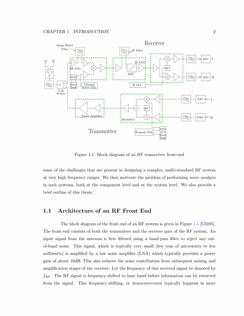
Figure 1.1: Block diagram of an RF transceiver front-end
some of the challenges that are present in designing a complex, multi-standard RF system
at very high frequency ranges. We then motivate the problem of performing noise analysis
in such systems, both at the component level and at the system level. We also provide a
brief outline of this thesis.
1.1 Architecture of an RF Front End
The block diagram of the front end of an RF system is given in Figure 1.1 [GM95].
The front end consists of both the transmitter and the receiver part of the RF system. An
input signal from the antenna is first filtered using a band-pass filter to reject any out-
of-band noise. This signal, which is typically very small (few tens of microwatts to few
milliwatts) is amplified by a low noise amplifier (LNA) which typically provides a power
gain of about 10dB. This also reduces the noise contribution from subsequent mixing and
amplification stages of the receiver. Let the frequency of this received signal be denoted by
fRF . The RF signal is frequency-shifted to base band before information can be retrieved
from the signal. This frequency-shifting, or downconversion typically happens in more

CHAPTER 1. INTRODUCTION 3
than one stage. This is due to the fact that the frequency of the received signal is of the
order of few gigahertz whereas the base band signal has bandwidth of a few kilohertz which
makes downconversion in one stage very expensive. Input RF signal is mixed with a large
local oscillator signal of frequency fLO and gets downconverted to a fixed intermediate
frequency signal fIF where fIF = |fRF − fLO|. This allows channel selection filtering and
gain control at lower frequencies where high quality factor (Q) filters and variable gain
amplifiers can be realized economically [FM99]. By varying the frequency of the local
oscillator signal, channels at different frequency band can be downconverted to the same
intermediate frequency. By the very nature of the process of downconversion, input signals
of frequency 2fLO − fRF , called the image frequency, also get downconverted to the same
intermediate frequency. Hence the RF mixer is preceded by a band-pass filter, called the
image-reject filter, which rejects the signals at the image frequency. This is usually a
ceramic filter which is implemented off chip. Since the LNA and the RF mixer operate
at RF frequencies, they are implemented on a separate chip using Gallium Arsenide or
specialized high speed bipolar technology.
The intermediate frequency signal is amplified and filtered to remove any signal
outside the desired band. Since the intermediate frequency of a typical RF system is fixed,
the IF filter need not be tunable and hence can be implemented with an extremely sharp
cutoff. Surface acoustic wave (SAW) filters are typically used for this purpose. The filtered
signal is mixed with the IF local oscillator signal and both the in-phase and quadrature
components of the signal get downconverted to base band. These are filtered using a low
pass filter to remove any undesired high frequency signal which would be folded to base
band during the subsequent sampling and digitization. The intermediate frequency range is
in few tens of megahertz and typically these circuits are implemented in standard BiCMOS
or CMOS technology.
In the transmit path, the in-phase and quadrature signals are upconverted to
RF frequency using a transmit phase lock loop (PLL). This signal is amplified using a
power amplifier before it drives the antenna. Due to power levels required and frequency
of operation, the upconversion mixer and the power amplifier are implemented on separate
chips using Gallium Arsenide or specialized high speed bipolar technology.
This architecture usually is implemented in four or five different chips which use
several different technologies, ranging from Gallium Arsenide and high speed bipolar to
digital CMOS technology. It also consists of some off chip ceramic and SAW filters. This

CHAPTER 1. INTRODUCTION 4
increases the power consumption and cost of the overall system. Every time an RF signal
is driven off chip, the output stage needs to drive the impedance of the lines on a PC board
which is typically 50Ω. This incurs extra power dissipation. Hence to increase battery life,
the trend in current RF designs is to minimize the number of times high frequency signals
need to be driven off chip. This is achieved by integrating more and more components
at radio and intermediate frequency of both the transmitter and the receiver on the same
silicon die. For designing RF systems which can be used for multiple standards, it is
also desirable to digitize the signal at as high a frequency as possible and perform IF
downconversion and other signal processing steps in the digital domain. With scaling of
digital CMOS technology, the digital portions of RF circuits are getting faster, which also
enables intermediate frequency operations to be performed in the digital domain. The block
diagram of a future, highly integrated RF transceiver is shown in Figure 1.2 [GM95]. In
such an architecture, the number of off chip elements is very small. The main objective
is to replace the functions traditionally implemented by high performance, high-Q discrete
components with integrated on-chip solutions [RON+98]. For instance, noise and image
rejection is performed using active components and channel-select synthesizer is realized
using on-chip active and passive components.
A direct consequence of this high integration is that the number of active and
passive devices, not just in the RF portion of the system, but also the signal path is
increasing. Unlike the digital portion of the system, which can be automatically synthesized
using digital synthesis techniques, the RF portion is still designed manually. The increasing
number of active and passive devices in this portion causes a dramatic increase in the
complexity of the design process and RF front end design is becoming more and more of a
bottleneck in the design of the overall communication system. Moreover, high integration
typically results in components with inferior performance as compared to their discrete
counterparts. For instance, on-chip VCOs which are used in the channel-select synthesizer
have much inferior phase noise performance compared to a VCO with high Q off-chip passive
elements [ROC+97]. This further exacerbates the design process complexity and leaves little
room for over-design.
To enable ease of design at the component level, efficient simulation techniques at
the transistor level are required which can effectively handle large circuits with a number
of devices operating in their strong nonlinear region. Additionally, in the initial stage of
design, transistor level description of the entire system may not be available. Hence compact

CHAPTER 1. INTRODUCTION 5
filtering
filtering
ADC
ADC Sync outClk outDout
Din
Control
Clk in
RFFilter
LNA Mixer
Mixer
Mixer Baseband gain
Baseband gain 10b 10MS/s
10b 10MS/s
Carrier trackingSymbol timing recoveryFrame recoverySymbol decodeSequqnce Correl.EqualizationAGC ControlDC Offset Control
Transmit pulseshaping
Trasmit burstcontrolChannel selectHopping controlPower adaptation
Amplifier
IF Channel SelectPLL Synthesizer
AdaptiveBasebandProcessor
Power Modulator
VCO1 VCO2
RF PLL
Xtal Oscillator
Filters
Filters DAC
DAC
Figure 1.2: Future high integration RF front-end
models of various components, along with behavioural level simulation techniques which use
these models, are required. These enable a system designer to quickly evaluate different
architectures and choose the one that is best suited for the current set of specifications. The
models should therefore be complete, so as to capture all the important effects which have
an impact on system performance, and compact so that the behavioural level simulation
algorithm does not become excessively slow.
Behavioural level simulation must be able to capture all significant interactions
between different components of the system so that the sensitivity of overall system perfor-
mance to specifications of a particular component performance can be accurately predicted.
More importantly, the change required in the specifications of other components of the
system, in order to maintain the overall system performance when the specification of one
component is changed, must also be predicted accurately. This enables a system designer
to investigate various design trade-offs at the behavioural level in a more systematic and
meaningful manner. Even at the later stage of a design, when the transistor level netlist
for the entire RF system might be available, it is prudent to extract these models from the
transistor level description of various components and use a behavioural level simulation

CHAPTER 1. INTRODUCTION 6
technique using these models.
1.2 Motivation
One of the reasons why RF front-end design is a bottleneck is that noise perfor-
mance is a very important part of high level specifications of an RF transceiver. Unlike
digital circuits where noise is a second order effect, noise in RF circuits directly affects high
level system performance such as signal to noise ratio (SNR) or the overall bit error rate
(BER). Noise also affects how the system SNR degrades in presence of a large adjacent
channel blocker signal. In the transmit path, it affects how much noise power the system is
leaking into adjacent channels [Pat96].
Roughly speaking noise refers to any unwanted change in signals in a circuit. For
instance, in a digital circuit, noise refers to any deviation of a signal from a logic zero (which
typically is 0V) or a logic one (which typically is the supply voltage VDD). In an RF circuit,
noise refers to any unwanted signal coupled into the circuit as well as unwanted signals
generated by the devices themselves.
1.2.1 Noise Sources in RF Transceiver
In a highly integrated transceiver, switching signals from digital portions of the
circuit can couple into sensitive RF circuit nodes and directly degrade the overall signal
to noise ratio. This coupling can happen through power supply lines as well as substrate.
However, careful design and layout techniques can minimize the effect of this coupling. By
ensuring separate power supply and ground for digital and RF portions of the system, using
a large bypass capacitance to remove any unwanted high frequency signals on the supply
network and by making the resistance of power supply to the RF portions very low, switching
noise coupled through the power supply can be minimized. Several techniques have been
proposed in the literature to minimize the amount of coupling from substrate [Gha96].
These usually involve using grounded guard rings around the sensitive RF circuits. For
different substrates, different topologies of guard rings can be used to minimize the amount
of signal that is coupled through the substrate [Gha96].
Another type of noise that has a detrimental effect on the system performance is
electrical noise which is intrinsic to electronic devices that make up the circuit itself. The

CHAPTER 1. INTRODUCTION 7
discrete nature of charge transfer gives rise to shot noise whenever the current crosses a
potential barrier. Shot noise is modelled as a zero mean stochastic process.
For a general one-dimensional stochastic process X(t), the autocorrelation, as a
function of two time variables t and τ , is given by
Rxx(t, τ) = E [X(t)X(t+ τ)]
If Rxx(t, τ) is independent of t, the stochastic process is called wide-sense stationary. For a
wide-sense stationary stochastic process, the power spectral density, i.e., power Sxx(ω) in a
unit frequency range at an angular frequency ω is given by
Sxx(ω) =∫ ∞−∞
Rxx(τ) exp(−ωτ)dτ
The spectral density of shot noise is given by
Sxx,shot(ω) = 2qId (1.1)
where q is the electron charge and Id is the current. The power spectral density is constant
for a very large frequency range (few tens of gigahertz) and hence can be modelled as
a scaled white noise source with power spectral density given in (1.1). White noise is a
mathematical idealization of this stochastic process. A white noise process is one which has
unit power spectral density for all frequencies.
Nyquist theorem shows that the short circuit current in a resistor, which is in
thermodynamic equilibrium, is a zero mean stochastic process. The power spectral density
of the output noise, called thermal noise is given by
Sxx,thermal(ω) = 4kTR (1.2)
where k is the Boltzmann’s constant, T is equilibrium temperature and R is the resistance.
The power spectral density is constant for a very large frequency range before dropping to
zero. Hence this noise process is also modelled as a scaled white noise process.
Another source of noise in devices is the flicker or 1/f noise. The physical origin
of this noise is due to random capture and release of charge by surface impurities. Due
to this noise generation method, noise power spectral density is typically much larger for
lower frequencies than higher frequencies. The noise power spectral density for this process
is given by
Sxx,flicker(ω) ∝ 1ωb
(1.3)
CHAPTER 1. INTRODUCTION 8
where b is 1 for typical flicker noise processes and ω is the angular frequency. This type
of noise represents a problem for noise modelling since the integrated noise power in any
finite band of frequencies around ω = 0 is infinite which is clearly unphysical [Wei93]. A
popular model of flicker noise is a stochastic process whose spectral density flattens out
at a finite and small frequency. This can be modelled as a series of filtered white noise
processes [MK82]. We will postpone further discussion of modelling flicker noise for now.
In this work we address the problem of analyzing the effect of electrical noise in RF
circuits. Specifically we address the problem of noise analysis in presence of additive white
noise sources. We use the mathematical idealization of a white noise source and formulate
the problem of noise analysis in nonlinear RF circuits as solutions of appropriate stochastic
differential equations. Given the specific nature of these stochastic differential equations,
we enumerate various properties of the solutions and develop compact and accurate math-
ematical models for RF components.
1.2.2 Autonomous versus Nonautonomous Circuits
For the purpose of noise analysis, we divide components present in a typical RF
system into two broad categories, autonomous and nonautonomous circuits. Autonomous
circuits are those which have no inputs (except for DC power supplies) and produce a (usu-
ally) periodic output. Typical examples of such circuits in an RF front-end are oscillators.
Nonautonomous circuits on the other hand will produce an interesting output only if sup-
plied with one or more inputs. Typical examples of such components in an RF front end
are mixers, filters, amplifiers etc.
Noise in autonomous oscillators is an important topic of investigation in itself.
A noiseless oscillator is supposed to provide a perfect time reference to the circuit. How-
ever since the oscillator output is corrupted by noise, it is not perfectly periodic and it
is said to have phase noise. Predicting phase noise in oscillators which are present in an
RF system is extremely important because it critically affects the overall system noise per-
formance [Nez98, Tom98, HKK98, VV83, Rob82]. Consider the frequency plot shown in
Figure 1.3. The desired channel that needs to be down-converted is showed as a solid ar-
row. Due to phase noise in the local oscillator, the oscillator output spectrum is not a
delta function, but is spread around the frequency of oscillation. If an adjacent channel
is also transmitting at the same time (shown as broken arrow), since the noisy oscillator

CHAPTER 1. INTRODUCTION 9
ω
Phase Noise Spectrum
DesiredChannel
ωBaseband
downconverted−→
ChannelAdjacent
Figure 1.3: Effect of oscillator phase noise on blocking performance
output power spectral density is nonzero at this adjacent channel frequency, the adjacent
channel also gets down-converted to base band, thereby directly degrading the overall SNR
of the system. Similarly in the transmit path, phase noise in local oscillator output causes
the upconverted signal to have finite energy outside the desired channel. Hence predicting
oscillator output noise is an important problem in its own right.
1.3 Thesis Overview
This dissertation is organized in the following manner: In Chapter 2 we present
a mathematical framework for performing noise analysis for RF circuits, both autonomous
and nonautonomous. We classify some of the existing noise analysis techniques in this
framework. We observe that traditional noise analysis of RF circuits is based on linear
perturbation analysis. We then show that this analysis cannot be carried over to oscil-
latory circuits since linear perturbation analysis is not valid for autonomous system of
equations (Chapter 3). We develop a new perturbation analysis technique for oscillatory
system of equations that is valid for deterministic perturbations. We obtain a nonlinear
differential equation for phase error of oscillators. For white noise perturbations, this dif-
ferential equation becomes a stochastic differential equation (Chapter 4). We use standard
techniques from stochastic differential equation theory to obtain a second order character-
ization of phase error and oscillator output as a stochastic process. The new oscillator
phase noise characterization forces us to revisit the traditional noise analysis techniques for
nonautonomous circuits which are driven by periodic signal which are derived from real os-
cillators and hence have phase noise. We address this problem in Chapter 5. We extend this
analysis (Chapter 6) to nonautonomous circuits which are driven by more than one large
periodic signals with incommensurable frequencies. We conclude (Chapter 7) by pointing

CHAPTER 1. INTRODUCTION 10
out some future directions where we believe this research can be extended.

11
Chapter 2
Overview of Existing Techniques
In this chapter we review some of the existing noise analysis techniques for au-
tonomous and nonautonomous circuits. We begin by describing a general framework of
noise analysis of nonautonomous circuits. We review some of the existing noise analysis
techniques based on this framework. We then review existing noise analysis techniques for
oscillators. We conclude by briefly describing our approach and contrasting them against
existing techniques.
2.1 Perturbation Analysis of a Nonoscillatory System
The behaviour of a nonlinear electronic circuit can be described by the following
system of differential equations
dq(x(t))dt
+ f(x(t)) + b(t) = 0 (2.1)
In this equation x(·) : R→ Rn represents a vector of state variables which, for an electronic
circuit, are node voltages and branch currents of voltage sources and inductors. q(·) : Rn →Rn represents the nonlinear charge and flux storage elements in the circuit, f(·) : Rn → R
n
represents memoryless nonlinearities in the circuit and b(·) : R → Rn represents inputs to
the nonautonomous circuit. RF circuits are usually analyzed for their steady-state response
for one or more periodic inputs. For the purpose of our analysis we assume that b(t) is a
large periodic signal with period T . By large we imply that the application of b(t) causes
the circuit operating point to change appreciably as a function of time. We assume that
the steady-state response of this circuit is given by xs(t), i.e., xs(t) satisfies (2.1). Since

CHAPTER 2. OVERVIEW OF EXISTING TECHNIQUES 12
the circuit is nonautonomous, xs(t) is also periodic with period T . Now we assume that
the circuit equations are perturbed by a perturbation term D(x)b(t). D(·) : Rn → Rn×p
is state dependent modulation term and b(·) : R → Rp is the state independent (but time
dependent) perturbation term. I.e., the perturbed system of equations is given by
dq(x(t))dt
+ f(x(t)) + b(t) +D(x)b(t) = 0 (2.2)
Let z(t) be the solution of (2.2). Linear perturbation analysis proceeds by assuming that
the response z(t) can be represented as
z(t) = xs(t) + xp(t) (2.3)
and for small perturbation term D(x)b(t), the deviation term xp(t) is small and bounded
for all t. Substituting the form of the solution (2.3) in (2.2) we have
dq(xs(t) + xp(t))dt
+ f(xs(t) + xp(t)) + b(t) +D(xs(t) + xp(t))b(t) = 0 (2.4)
Since xp(t) is assumed to be small, the nonlinear functions q and f can be linearized around
the periodic steady-state solution xs(t) and (2.4) can be written as
ddt
(q(xs(t)) +
dq(x)dx
∣∣∣∣xs(t)
xp(t)
)+ f(xs(t)) +
df(x)dx
∣∣∣∣xs(t)
xp(t) + b(t) +D(xs(t))b(t) = 0
Here we have ignored xp(t) in the argument of D(·). We use only the zeroth order Taylor
series term B(xs)b(t) which captures the modulation of the perturbation sources with the
large signal steady state and ignore the first order term in the expansion of B(x)b(t) around
xs(t), i.e.,
dD(x)dx
∣∣∣∣xs(t)
xp(t)b(t)
This term is a high-order effect that captures the modulation of the perturbation sources
with themselves and can be neglected for all practical purposes. Since xs(t) is the solution
of (2.1), we obtain
ddt
(C(t)xp(t)) +G(t)xp(t) +D(xs(t))b(t) = 0 (2.5)
where
C(t) =dq(x)
dx
∣∣∣∣xs(t)

CHAPTER 2. OVERVIEW OF EXISTING TECHNIQUES 13
and
G(t) =df(x)
dx
∣∣∣∣xs(t)
and C(t) and G(t) are T -periodic. (2.5) can be rewritten as
C(t)xp(t) +A(t)xp(t) +D(xs(t))b(t) = 0 (2.6)
where A(t) = G(t)+ C(t). For a typical circuit, C(t) need not be full rank and hence not all
entries of xp(t) are independent of each other. (2.6) is a differential equation that is linear
in xp(t) and the coefficient matrices A(t) and C(t) are T -periodic. Hence the homogeneous
part of (2.6) describes a linear periodic time varying (LPTV) transfer function h(t1, t2).
Once h(t1, t2) is obtained, the output xp(t) can be obtained by the following convolution
integral
xp(t) =∫ ∞−∞
h(t, s)D(xs(s))b(s)ds
2.2 Noise Analysis of Nonoscillatory Systems
For stochastic perturbations, specifically for white noise perturbations b(t) = ξ(t),
(2.6) is a stochastic differential equation and xp(t) is now a stochastic process. (2.6) is
written in the stochastic differential form as follows [Øks98]
C(t)dxp(t) +A(t)xp(t)dt+D(xs(t))dB(t) = 0 (2.7)
where B(t) is a p-dimensional Brownian motion process. It can be shown that this linear
differential equation has a solution of the form
xp(t) =∫ ∞−∞
h(t, s)D(xs(s))dB(s)
where the integral in the above equation is to be interpreted as a stochastic integral [Øks98].
Hence
E
[xp(t1)xTp (t2)
]= E
[∫ ∞−∞
h(t1, s1)D(xs(s1))dB(s1)∫ ∞−∞
dBT (s2)DT (xs(s2))hT (t2, s2)]
=∫ ∞−∞
∫ ∞−∞
h(t1, s1)D(xs(s1))E[dB(s1)dBT (s2)
]DT (xs(s2))hT (t2, s2)
=∫ ∞−∞
h(t1, s)D(xs(s))DT (xs(s))hT (t2, s)ds

CHAPTER 2. OVERVIEW OF EXISTING TECHNIQUES 14
Existing noise analysis techniques take advantage of the fact that the transfer function is
linear periodic time varying and hence satisfies the relation
h(t1, t2) = h(t1 + T, t2 + T )
This implies that for stationary input noise (i.e., the second order statistics do not change
with time) or cyclostationary input noise (i.e., the second order statistics are periodic with
the same period T ), the output noise is also cyclostationary. Noise statistics for one period
are directly computed from (2.7). There are several techniques proposed in the literature
which perform this computation either in time domain or in frequency domain.
2.2.1 LPTV Approaches and Extensions
Noise analysis of nonlinear RF components driven by one or more periodic sig-
nals, has been a focus of attention of several researchers. One of the earliest efforts was
concentrated on noise analysis of millimeter wave mixers [HK77]. Earlier works concen-
trated on extending traditional linear time invariant noise analysis techniques to weakly
nonlinear circuits [RPP88]. Target circuits for these approaches were almost invariably
high frequency mixers [RMC89]. Efforts were made later to extend this noise analysis to
strongly nonlinear components present in RF front ends [HKW91, Hud92] and with arbitrary
topologies [RM92]. Earlier efforts concentrated on microwave circuits which were predom-
inantly linear with very few nonlinear elements [OTS91, RMM92b, RMM92a, RMM94b,
RMM94a, RMM95, RMC98]. Since then, techniques have been suggested to speed up
Newton iteration and the solution of the underlying large linear system of equations us-
ing iterative linear algebra techniques [RFL98]. These techniques can also address the
problem of noise analysis of nonautonomous circuits driven by two or more large periodic
signals [RMM94b, RMM94a, RFL98]. Though frequency domain techniques, usually based
on harmonic balance, are more popular for RF circuits, several time domain techniques
have also been suggested [Hul92, HM93, TKW96]. All these techniques usually concentrate
on analyzing noise performance of nonlinear nonautonomous circuits assuming perfect LO
input. The underlying assumption is that a noisy oscillator output can be viewed as a de-
terministic, large, perfectly periodic signal with additive amplitude and phase noise. With
this assumption, input signal noise can be absorbed in the circuit and can be viewed as a
circuit noise source [RMMN92]. However, as we will see in Chapter 3, this representation

CHAPTER 2. OVERVIEW OF EXISTING TECHNIQUES 15
is not valid for real oscillator output. Therefore we need to revisit the problem of noise
analysis of nonautonomous circuits in presence of input signal phase noise.
2.2.2 Time Domain Analysis
In [DLSV96], a technique for numerically solving (2.7) as a stochastic differential
equation is presented. No assumption is made about the nature of inputs. From (2.7),
an ordinary differential equation for the variance E[x(t)xT (t)
]and the autocorrelation
E
[x(t1)xT (t2)
]is derived. These equations are solved numerically using transient simulation
algorithm in Spice. Circuit noise sources are modelled as white noise processes. This
technique is used to compute output noise of a bipolar active mixer (along with several
other circuits). Since input to the mixer is assumed to be perfectly periodic, the output
noise variance is calculated to be periodically varying with time. However, no provision
has been made to account for input signal phase noise in the simulation algorithm. Several
other time domain noise analysis techniques have also been proposed which use different
numerical integration techniques for stochastic differential equations [SD98, Dob93].
2.2.3 Our Approach
Existing techniques for noise simulation for nonautonomous circuits do not take
into account the effect of input signal phase noise. If the input signal is noiseless and per-
fectly periodic, the output noise is cyclostationary as would be predicted by these existing
techniques. However, the input signal is derived from a real signal source (oscillator) and
therefore has phase noise. A noisy periodic signal does not provide a perfect time reference.
Therefore noise in a circuit driven by such a signal cannot be cyclostationary. Cyclosta-
tionarity of output noise implies that its statistics vary perfectly periodically with time, i.e.,
provide a perfect time reference.
We formulate the problem of performing noise analysis of nonautonomous circuits
driven by large periodic signals with phase noise as the solution of a stochastic differential
equation. We show that
• The output of nonlinear nonautonomous systems in the presence of period input with
Brownian motion phase deviation, is asymptotically wide sense stationary.
• The Lorentzian spectrum of the input signal and the characteristics of the Brownian
motion input phase deviation process are preserved at the output.
CHAPTER 2. OVERVIEW OF EXISTING TECHNIQUES 16
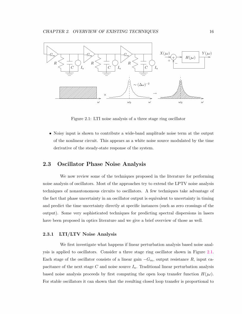
−Gm
RC In
−Gm
RC In
−Gm
RC In
ωω0 ω0
× →
∼ (∆ω)−2
ωω
++−
Y (ω)X(ω)H(ω)
Figure 2.1: LTI noise analysis of a three stage ring oscillator
• Noisy input is shown to contribute a wide-band amplitude noise term at the output
of the nonlinear circuit. This appears as a white noise source modulated by the time
derivative of the steady-state response of the system.
2.3 Oscillator Phase Noise Analysis
We now review some of the techniques proposed in the literature for performing
noise analysis of oscillators. Most of the approaches try to extend the LPTV noise analysis
techniques of nonautonomous circuits to oscillators. A few techniques take advantage of
the fact that phase uncertainty in an oscillator output is equivalent to uncertainty in timing
and predict the time uncertainty directly at specific instances (such as zero crossings of the
output). Some very sophisticated techniques for predicting spectral dispersions in lasers
have been proposed in optics literature and we give a brief overview of those as well.
2.3.1 LTI/LTV Noise Analysis
We first investigate what happens if linear perturbation analysis based noise anal-
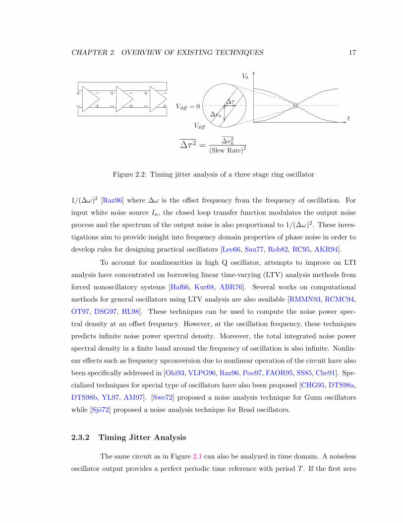
ysis is applied to oscillators. Consider a three stage ring oscillator shown in Figure 2.1.
Each stage of the oscillator consists of a linear gain −Gm, output resistance R, input ca-
pacitance of the next stage C and noise source In. Traditional linear perturbation analysis
based noise analysis proceeds by first computing the open loop transfer function H(ω).
For stable oscillators it can shown that the resulting closed loop transfer is proportional to
CHAPTER 2. OVERVIEW OF EXISTING TECHNIQUES 17
∆τ 2 = ∆v2n
(Slew Rate)2
− + +
−
−
−
Vdiff = 0∆τ
∆vn
−
V0
t
−
+
+ + +
Vdiff
Figure 2.2: Timing jitter analysis of a three stage ring oscillator
1/(∆ω)2 [Raz96] where ∆ω is the offset frequency from the frequency of oscillation. For
input white noise source In, the closed loop transfer function modulates the output noise
process and the spectrum of the output noise is also proportional to 1/(∆ω)2. These inves-
tigations aim to provide insight into frequency domain properties of phase noise in order to
develop rules for designing practical oscillators [Lee66, Sau77, Rob82, RC95, AKR94].
To account for nonlinearities in high Q oscillator, attempts to improve on LTI
analysis have concentrated on borrowing linear time-varying (LTV) analysis methods from
forced nonoscillatory systems [Haf66, Kur68, ABR76]. Several works on computational
methods for general oscillators using LTV analysis are also available [RMMN93, RCMC94,
OT97, DSG97, HL98]. These techniques can be used to compute the noise power spec-
tral density at an offset frequency. However, at the oscillation frequency, these techniques
predicts infinite noise power spectral density. Moreover, the total integrated noise power
spectral density in a finite band around the frequency of oscillation is also infinite. Nonlin-
ear effects such as frequency upconversion due to nonlinear operation of the circuit have also
been specifically addressed in [Ohi93, VLPG96, Raz96, Poo97, FAOR95, SS85, Che91]. Spe-
cialized techniques for special type of oscillators have also been proposed [CHG95, DTS98a,
DTS98b, YL97, AM97]. [Swe72] proposed a noise analysis technique for Gunn oscillators
while [Sjo72] proposed a noise analysis technique for Read oscillators.
2.3.2 Timing Jitter Analysis
The same circuit as in Figure 2.1 can also be analyzed in time domain. A noiseless
oscillator output provides a perfect periodic time reference with period T . If the first zero

CHAPTER 2. OVERVIEW OF EXISTING TECHNIQUES 18
crossing of the oscillator output is synchronized to t = 0, then a noiseless oscillator output
will have a zero crossing at time t = kT , k ∈ Z+. Since a real oscillator output is corrupted
by noise, zero crossings will not exactly be at time t = kT . The variance of zero crossing
time is known as cycle to cycle jitter. Consider the three stage ring oscillator in Figure 2.2.
Variance in zero crossing is computed by calculating the voltage noise at the zero crossing
instance and dividing it by the square of the slew rate at that time. There are techniques
proposed in the literature [WKG94, McN97] which compute the voltage variance assuming
idealized models of specific kinds of delay cells that are used in the ring oscillator. Similar
techniques [AM83] are proposed for oscillators with regenerative switching (or relaxation
oscillator). The mechanisms of such oscillators suggest the fundamental intuition that
timing or phase errors increase with time. These technique become extremely involved if
realistic models for delay cells are used. It is also not clear how to extend these techniques
to compute phase noise in nonswitching (harmonic) oscillators.
2.3.3 Time Domain Noise Analysis
Demir et. al. [DSV96] used their time domain non-Monte Carlo noise simulation
algorithm [DLSV96] to compute the noise in an oscillator output. The noise simulation
technique is also based on linear perturbation analysis. They concluded that the envelop of
the variance of output noise power keeps increasing unbounded with time. This result, in
some sense, is the time domain equivalent interpretation of the result derived in Section 2.3
which predict infinite integrated power of oscillator output noise. The reason why both
these techniques show this unphysical result is because they are based on linear perturbation
analysis which is not valid for oscillators.
2.3.4 Other Approaches
More sophisticated analysis techniques exist in optics. Here, stochastic analysis is
common and it is well known that that phase error in oscillators, due to white noise sources,
is described by a Brownian motion process. Although justifications of this fact are often
based on approximations, precise descriptions of phase noise have been obtained for certain
systems. In the seminal work of Lax [Lax67], an equation describing the growth of phase
fluctuations with time is obtained for pumped lasers. The fact that a Brownian motion phase
error process leads to Lorentzian output power spectrum is also well established [FV88,

CHAPTER 2. OVERVIEW OF EXISTING TECHNIQUES 19
VV83]. However, a general theory is not available in this field as well.
There are a few approaches which are based on nonlinear analysis of the oscilla-
tor dynamics [Dek87, Gol89]. Possibly the most general and rigorous treatment of phase
noise has been that of [Kar90]. Using several novel methods, the oscillator response is
decomposed into phase and amplitude variation and a nonlinear differential equation for
phase error is obtained. By solving a linear, small time approximation to this equation with
stochastic inputs, a Lorentzian spectrum due to white noise is obtained. In spite of these
advances, certain gaps remain, particularly with respect to the derivation and solution of
the differential equation governing phase error.
2.3.5 Our Approach
Our approach for oscillator phase noise analysis can be summarized as follows:
• As a first step, we develop a new quantitative description of the dynamics of stable
nonlinear oscillators in presence of deterministic perturbations which is not limited to
two-dimensional system of equations and does not make any assumptions about the
type of nonlinearity.
• By considering stochastic perturbations in a stochastic differential calculus setting,
we obtain a correct mathematical characterization of the noisy oscillator output.
• We show that the oscillator output is represented as the sum of two stochastic pro-
cesses: a large signal output with Brownian motion phase deviation and a small
“amplitude” noise process.
• We further show that the response of the noisy oscillator is asymptomatically wide-
sense stationary with Lorentzian power spectral density.

20
Chapter 3
Perturbation Analysis of Stable
Oscillators
As pointed out in Chapter 2, noise analysis in electrical circuits is based on pertur-
bation analysis. It is well known that linear perturbation analysis is not valid for oscillatory
circuits. In order to develop a noise analysis technique for oscillators we first need to develop
a rigorous perturbation analysis technique. In this chapter we first show that traditional
linear perturbation analysis is not valid for oscillators. This also helps us introduce the
notations which we use when we describe our perturbation analysis technique. We show
that this incorrect linearization leads to nonphysical results such as infinite oscillator output
phase noise power in presence of white noise. We then describe our perturbation analysis
technique in detail. This analysis is not limited to any specific type electrical oscillator. In
fact this analysis is valid for any autonomous system of equations with oscillatory solution.
We also demonstrate our technique with an example.
3.1 Mathematical Preliminaries
The dynamics of any autonomous system without undesired perturbations can be
described by a system of differential equations:1
x = f(x) (3.1)
1For notational simplicity, we use the state equation formulation to describe the dynamics of an au-tonomous system. The results we present can be easily extended to mixed differential-algebraic formulationgiven by dq(x)
dt+ f(x) = 0.
CHAPTER 3. PERTURBATION ANALYSIS OF STABLE OSCILLATORS 21
where x ∈ Rn and f(·) : Rn → Rn. We assume that f(·) satisfies the conditions of the
Picard-Lindelof existence and uniqueness theorem for initial value problems [Far94]. We
assume that solution of (3.1), xs(t) is periodic with period T and describes an asymptotically
orbitally stable limit cycle in the n-dimensional solution space. We explain the concept of
asymptotic orbital stability below [Far94].
Since xs(t) is a solution of (3.1), xs(t−t0) is also a nonconstant T -periodic solution
for arbitrary t0 ∈ R. The initial values xs(0) and xs(−t0) can be arbitrarily close (if |t0| is
small enough), and still xs(t) − xs(t − t0) does not tend to zero as t tends to infinity. Let
the path γ of the T -periodic solution xs(t) be
γ = x ∈ R : x = xs(t), t ∈ R+
We note that xs(t) and xs(t− t0) have the same path γ.
Definition 3.1 (Orbital Stability) The solution xs(t) of (3.1) is said to be orbitally
stable if for every ε > 0, there exists a δ(ε) such that if the distance of the initial value
x(0) = x0 from the path γ of xs(t) is less than δ(ε), i.e., dist(x0, γ) < δ(ε), then the solution
φ(t, x0) of (3.1) that assumes the value x0 at t = 0 satisfies
dist(φ(t, x0), γ) < ε
for t ≥ 0.
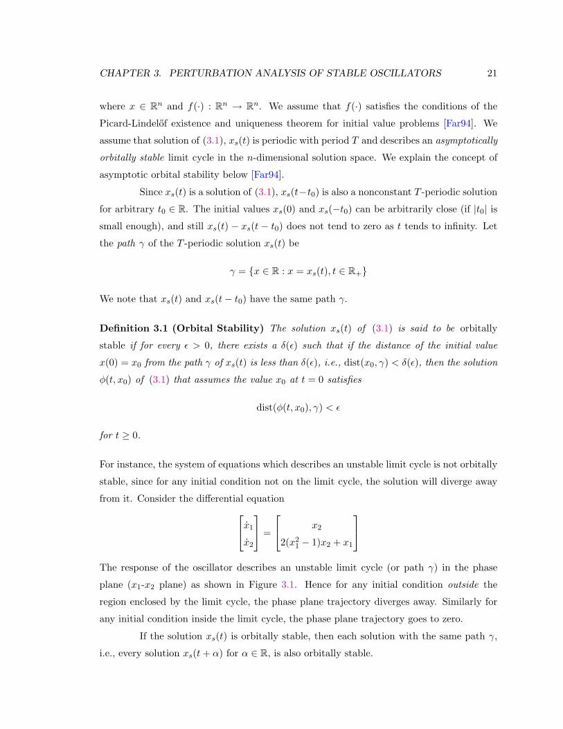
For instance, the system of equations which describes an unstable limit cycle is not orbitally
stable, since for any initial condition not on the limit cycle, the solution will diverge away
from it. Consider the differential equationx1
x2
=
x2
2(x21 − 1)x2 + x1
The response of the oscillator describes an unstable limit cycle (or path γ) in the phase
plane (x1-x2 plane) as shown in Figure 3.1. Hence for any initial condition outside the
region enclosed by the limit cycle, the phase plane trajectory diverges away. Similarly for
any initial condition inside the limit cycle, the phase plane trajectory goes to zero.
If the solution xs(t) is orbitally stable, then each solution with the same path γ,
i.e., every solution xs(t+ α) for α ∈ R, is also orbitally stable.

CHAPTER 3. PERTURBATION ANALYSIS OF STABLE OSCILLATORS 22
−3 −2 −1 0 1 2 3−4
−3
−2
−1
0
1
2
3
x1(t)
x2(t
)
Figure 3.1: Response of an orbitally unstable oscillator
Definition 3.2 (Asymptotic Orbital Stability) The solution xs(t) of (3.1) is said to
be asymptotically orbitally stable if it is orbitally stable, and if a δ > 0 exists such that
dist(x0, γ) < δ implies
dist(φ(t, x0), γ)→ 0 as t→∞
Definition 3.3 (Asymptotic Phase Property) The solution xs(t) is said to have the
asymptotic phase property if a δ > 0 exists such that to each initial value x0 satisfying
dist(x0, γ) < δ there corresponds an asymptotic phase α(x0) ∈ R with the property
limt→∞|φ(t, x0)− xs(t+ α(x0))| = 0
A lossless LC tank with a finite energy stored in the tank is not an asymptotically
orbitally stable system. The response of the oscillator describes a closed orbit in two-
dimensional state space (formed by the capacitor voltage and inductor current). However,
if the oscillator is perturbed by a small instantaneous change in the system energy, the
system moves to a new limit cycle and never returns to its original limit cycle. Hence

CHAPTER 3. PERTURBATION ANALYSIS OF STABLE OSCILLATORS 23
this is not an asymptotically orbitally stable system. For the autonomous systems we are
dealing in this work, we assume that there exists a nontrivial periodic solution xs(t) which
is asymptotically orbitally stable, and has the asymptotic phase property.
We are interested in the response of such systems to a small state-dependent
perturbation of the form D(x)b(t) where D(·) : Rn → Rn×p and b(·) : R → R
p. I.e., the
perturbed system is described by
x = f(x) +D(x)b(t) (3.2)
Let the exact solution of the perturbed system in (3.2) be z(t).
3.2 Perturbation Analysis Using Linearization
The traditional approach to analyzing perturbed nonlinear systems is to linearize
about the unperturbed solution under the assumption that the resultant deviation, i.e., the
difference between the solutions of the perturbed and unperturbed systems, will be small.
Let this deviation be w(t), i.e.,
z(t) = xs(t) + w(t)
Substituting this expression in (3.2) we obtain
xs(t) + w(t) = f(xs(t) + w(t)) +D(xs(t) + w(t))b(t)
We assume that for “small” perturbations D(x)b(t) the resulting deviation w(t) will be
small. Hence, in the above expression we can approximate f(xs(t) +w(t)) by its first order
Taylor series expansion and replace D(xs(t) + w(t))b(t) with D(xs(t))b(t). Using these
approximations and observing that xs(t) satisfies (3.1), we obtain
w(t) ≈ ∂f(x)∂x
∣∣∣∣xs(t)
w(t) +D(xs(t))b(t)
= J(t)w(t) +D(xs(t))b(t)
(3.3)
where the Jacobian
J(t) =∂f(x)∂x
∣∣∣∣xs(t)
J : R→ Rn×n is T -periodic. We would like to solve for w(t) in (3.3) to see if our assumption
that it is small is indeed justified. (3.3) describes a linear periodically time-varying system

CHAPTER 3. PERTURBATION ANALYSIS OF STABLE OSCILLATORS 24
of equations governing the dynamics of w(t). For solving this equation we will use results
from Floquet theory [Far94, Gri90] which we describe below.
3.2.1 Floquet Theory
The homogeneous system of differential equations corresponding to (3.3) is given
by
w = J(t)w (3.4)
We begin by making the following observations:
Remark 3.1
• The conditions of the Picard-Lindelof existence and uniqueness theorem [Far94] for
initial value problems are trivially satisfied by (3.3) and (3.4). Hence, there exist
unique solutions to (3.3) and (3.4) given an initial condition w(t0) = w0.
• It can be shown that the set of real solutions of (3.4) form an n-dimensional linear
space.
• Let w1(t, t0), . . . , wn(t, t0) be n linearly independent solutions of (3.4). Then,
W (t, t0) = [w1(t, t0), . . . , wn(t, t0)]
is called a fundamental matrix. The fundamental matrix satisfies
dW (t, t0)dt
= J(t)W (t, t0)
If W (t0, t0) = I, the n× n identity matrix then W (t, t0) is called the principal funda-
mental matrix, or the state transition matrix for (3.4), denoted by Φ(t, t0).
• Any solution of (3.4) can be expressed as W (t, t0)c where c 6= 0 is a constant vector.
In particular, for w(t0) = x0, the solution of (3.4) is given by Φ(t, t0)x0.
• If W (t, t0) is another fundamental matrix for (3.4) then W (t, t0) = W (t, t0)C where
C is a nonsingular constant matrix.
• The solution w of (3.3) satisfying the initial condition w(t0) = w0 is given by
w(t, t0, x0) = Φ(t, t0)x0 +∫ t
t0
Φ(t, s)D(xs(s))b(s)ds

CHAPTER 3. PERTURBATION ANALYSIS OF STABLE OSCILLATORS 25
In the above observations we have not used the fact that the entries of J(t) are
periodic. Since for the case of a periodic oscillator, J(t) is T -periodic, J(t + T ) = J(t) for
all t ∈ R. Let W (t, t0) be a fundamental matrix for (3.4). We further observe that:
Remark 3.2
• If W (t, t0) is a fundamental matrix then for W (t+ T, t0), we have
W (t+ T, t0) = J(t+ T )W (t+ T, t0)
= J(t)W (t+ T, t0)
hence W (t+ T, t0) is also a fundamental matrix. Then,
W (t+ T, t0) = W (t, t0)B
where B is a nonsingular matrix and
B = W−1(t0, t0)W (t0 + T, t0)
Since the columns of W are linearly independent, the inverse in the above expression
exists.
• Even though B is not unique, it can be shown that any other B will have the same
eigenvalues.
• The (unique) eigenvalues of B, λ1, . . . , λn, are called the characteristic multipliers of
the equation (3.4) and the characteristic (Floquet) exponents µ1, . . . , µn are defined
as
λi = exp(µiT )
Assumption 3.1 We assume that B has distinct eigenvalues and it is diagonalizable2.
Now we state a result due to Floquet (1883):
Theorem 3.1 (Floquet) Let B be diagonalized as
B = ΞΛΞ−1
2The extension to nondiagonalizable matrices is straightforward.

CHAPTER 3. PERTURBATION ANALYSIS OF STABLE OSCILLATORS 26
where Λ = diag[λ1, . . . , λn]. Let
D = diag[µ1, . . . , µn]
where µi is defined as λi = exp(µiT ). Then, the state transition matrix of the system (3.4),
as a function of two variables, t and s = t0, can be written in the form
Φ(t, s) = U(t) exp(D(t− s))V (s) (3.5)
where U(t) and V (t) are both T -periodic and nonsingular, and satisfy
U(t) = V −1(t)
for all t.
Proof: We have
W (t+ T, s) = W (t, s)B
= W (t, s)ΞΛΞ−1
and hence
W (t+ T, s)Ξ = W (t, s)ΞΛ (3.6)
Let Y (t, s) = W (t, s)Ξ. Using this relation, (3.6) reduces to
Y (t+ T, s) = Y (t, s)Λ
= Y (t, s) exp(DT )
Since W (t, s) is nonsingular, Y (t, s) is also a fundamental matrix of (3.4). For a given s let
U(t) = Y (t, s) exp(−D(t− s))
and V (t) = U−1(t). We observe that
U(t+ T ) = Y (t+ T, s) exp(−D(t+ T − s))= Y (t, s) exp(DT ) exp(−D(t+ T − s))= Y (t, s) exp(−D(t− s))= U(t)
i.e., U(t) is T -periodic. Here we used the fact that for scalar s and t
exp(Ds) exp(Dt) = exp(Dt) exp(Ds) = exp(D(t+ s))
CHAPTER 3. PERTURBATION ANALYSIS OF STABLE OSCILLATORS 27
Hence both U(t) and V (t) are T -periodic. Let
Φ(t, s) = U(t) exp(D(t− s))V (s)
We note that Φ(s, s) = I and Φ(t, s) satisfies (3.4), hence Φ(t, s) is the state transition
matrix of (3.4).
Remark 3.3
• The state transition matrix Φ(t, s) can be written as
Φ(t, s) =[u1(t) . . . un(t)
]eµ1(t−s)
. . .
eµn(t−s)
vT1 (s)
...
vTn (s)
=
n∑i=1
exp (µi(t− s))ui(t)vTi (s)
where ui(t) are the columns of U(t), and vTi (t) are the rows of V (t) = U−1(t).
• With this representation of the state transition matrix, the solutions of the homoge-
neous system (3.4) and the inhomogeneous system (3.3) with a periodic coefficient
matrix are given by
wH(t) =n∑i=1
exp (µi(t− t0))ui(t)vTi (t0)x(t0)
and
wIH(t) = wH(t) +n∑i=1
ui(t)∫ t
t0
exp (µi(t− s))vTi (s)b(s)ds
• For any i, w(t) = ui(t) exp(µit) is a solution of (3.4) with the initial condition w(t0) =
ui(t0) exp(µit0). Similarly, w(t) = vi(t) exp(−µit) is a solution of the adjoint system
w = −JT (t)w
with the initial condition w(t0) = vi(t0) exp(−µit0).
• We have
Φ(T, 0) =n∑i=1
exp (µiT )ui(T )vTi (0)
=n∑i=1
exp (µiT )ui(0)vTi (0)
CHAPTER 3. PERTURBATION ANALYSIS OF STABLE OSCILLATORS 28
From the above, ui(0) are the eigenvectors of Φ(T, 0) with corresponding eigenval-
ues exp (µiT ), and vi(0) are the eigenvectors of Φ(T, 0)T corresponding to the same
eigenvalues.
3.2.2 Response to Deterministic Perturbation
We now use the results of Floquet Theory to obtain a solution w(t) of (3.3). The
state transition matrix of (3.4), the homogeneous part of (3.3), is given by (3.5) which is
repeated here
Φ(t, s) = U(t) exp(D(t− s))V (s)
Here U(t) is a T -periodic nonsingular matrix, V (t) = U−1(t) and D = diag[µ1, . . . , µn]
where where µi are the Floquet (characteristic) exponents and exp (µiT ) are the character-
istic multipliers.
Remark 3.4 Let ui(t) be the columns of U(t) and vTi (t) be the rows of V (t) = U−1(t).
Then u1(t), u2(t), . . . , un(t) and v1(t), v2(t), . . . , vn(t) both span Rn and satisfy the bi-
orthogonality conditions vTi (t)uj(t) = δij for every t. In general, U(t) itself is not an
orthogonal matrix.
Let us first consider the homogeneous part of (3.3), the solution of which is given
by
wH(t) = U(t) exp(Dt)V (0)w(0)
=n∑i=1
ui(t) exp(µit)vTi (0)w(0)
where w(0) is the initial condition. Next, we will show that one of the terms in the sum-
mation in the above equation does not decay with t.
Lemma 3.2
• The time-derivative of the periodic solution xs(t) of (3.1), i.e., xs(t), is a solution of
the homogeneous part of (3.3).
• The unperturbed oscillator (3.1) has a nontrivial T -periodic solution xs(t) if and only
if the number 1 is a characteristic multiplier of the homogeneous part of (3.3), or
equivalently, one of the Floquet exponents satisfies exp(µiT ) = 1.
CHAPTER 3. PERTURBATION ANALYSIS OF STABLE OSCILLATORS 29
Proof: Since xs(t) is a nontrivial periodic solution of (3.1), it satisfies
xs(t) = f(xs(t))
Taking the time derivative of both sides of this equation, we have
xs =∂f
∂x
∣∣∣∣xs(t)
xs
Hence, xs(t) satisfies w = J(t)w, the homogeneous part of (3.3). Thus,
xs(t) =n∑i=1
ui(t) exp(µit)vTi (0)xs(0)
Since xs(t) is periodic, it follows that at least one of the Floquet exponents satisfies
exp(µiT ) = 1.
Remark 3.5 One can show that if 1 is a characteristic multiplier, and the remaining n−1
Floquet exponents satisfy |exp(µiT )| < 1, i = 2, . . . , n, then the periodic solution xs(t) of
(3.1) is asymptotically orbitally stable and it has the asymptotic phase property [Far94].
This is a sufficient condition for asymptotic orbital stability, not a necessary one. We
assume that this sufficient condition is satisfied by the system and the periodic solution
xs(t). Moreover, if any of the Floquet exponents satisfy | exp (µiT )| > 1, then the solution
xs(t) is orbitally unstable.
Without loss of generality, we choose µ1 = 0 and u1(t) = xs(t).
Remark 3.6 With u1(t) = xs(t), we have
vT1 (t) xs(t) = 1
and
vT1 (t)uj(t) = 0 j = 2, . . . , n
v1(t) will play an important role in the rest of our treatment.
Next, we obtain the particular solution of (3.3), given by
wP (t) =∫ t
0U(t) exp(D(t− r))V (r)D(xs(r))b(r)dr
=n∑i=1
ui(t)∫ t
0exp(µi(t− r))vTi (r)D(xs(r))b(r)dr

CHAPTER 3. PERTURBATION ANALYSIS OF STABLE OSCILLATORS 30
Since exp(µ1T ) = 1, the first term in the above summation is given by
u1(t)∫ t
0vT1 (r)D(xs(r))b(r)dr
If the integrand has a nonzero average value, then the deviation w(t) in (3.3) will grow
unbounded. Hence, the assumption that w(t) is small becomes invalid and the linearization
based perturbation analysis is inconsistent.
Before we present our perturbation analysis technique for stable oscillators, we will
show that noise analysis of oscillators based on linear perturbation analysis is also invalid
and it leads to nonphysical results such as infinite total integrated noise power.
3.2.3 Response to Stochastic Perturbation
Now, we consider the case where the perturbation b(t) is a vector of uncorrelated
white noise sources ξ(t), i.e.,
E
[ξ(t1)ξT (t2)
]= Iδ(t1 − t2)
where E [·] denotes the probabilistic expectation operator and I is p×p identity matrix. We
now find the expression of the autocorrelation matrix
K(t) = E
[w(t)wT (t)
]of the solution of (3.3) for K(0) = 0. We have
K(t) = E
[w(t)wT (t)
]= E
[∫ t
0Φ(t, s1)D(xs(s1))ξ(s1)ds1
∫ t
0ξT (s2)DT (xs(s2))ΦT (t, s2)ds2
]=∫ t
0
∫ t
0Φ(t, s1)D(xs(s1))E
[ξ(s1)ξT (s2)
]DT (xs(s2))ΦT (t, s2)ds1ds2
=∫ t
0
∫ t
0Φ(t, s1)D(xs(s1))δ(s1 − s2)DT (xs(s2))ΦT (t, s2)ds1ds2
i.e.,
K(t) =∫ t
0Φ(t, s)D(xs(s))DT (xs(s))Φ(t, s)Tds (3.7)
If we substitute
Φ(t, s) =n∑i=1
exp (µi(t− s))ui(t)vTi (s)

CHAPTER 3. PERTURBATION ANALYSIS OF STABLE OSCILLATORS 31
in (3.7) we obtain
K(t) =n∑i=1
n∑j=1
ui(t)uTj (t)[∫ t
0exp((µi + µj)t)vTi (s)D(xs(s))DT (xs(s))vj(s)ds
]
Since exp(µ1T ) = 1, the term in the summation above for i = j = 1 is given by
u1(t)uT1 (t)[∫ t
0vT1 (s)D(xs(s))DT (xs(s))v1(s)ds
]The integrand vT1 (s)D(xs(s))DT (xs(s))v1(s) is a nonnegative scalar that is periodic in s
sinceD(xs(s))DT (xs(s)) is a positive semi-definite matrix. This scalar has a positive average
value, hence this term grows unbounded with t. Thus, the assumption that the deviation
w(t) stays small is also invalid for the stochastic perturbation case, because the variances
of the entries of w(t) can grow unbounded. The notion of “staying small” is quite different
for a stochastic process than the one for a deterministic function. For instance, a Gaussian
random variable can take arbitrarily large values with nonzero probability even when its
variance is “small”. We say that a stochastic process is “bounded” when its variance is
bounded, even though some of its sample paths (representing a nonzero probability) can
grow unbounded.
3.3 Nonlinear Perturbation Analysis for Phase Deviation
As seen in the previous section, traditional perturbation techniques do not suffice
for analyzing oscillators. In this section, we develop a novel nonlinear perturbation analysis
suitable for oscillators. Before we present the mathematical details we will explain the
intuition behind our approach. Consider the unperturbed oscillator output which describes
a stable limit cycle. When a perturbation is applied to the oscillator, this periodicity is
lost. For stable oscillators, however, the perturbed trajectory remains within a small band
around the unperturbed trajectory as shown in Figure 3.2.
The proximity of the perturbed and unperturbed trajectories in the phase plane
does not imply that the time-domain waveforms are also close to each other. At a given
time t, the unperturbed oscillator output xs(t) and the perturbed oscillator output z(t),
can be far from each other as illustrated in Figure 3.2. This further indicates that the
linear perturbation analysis which concludes that the deviation w(t) = z(t) − xs(t) grows
unbounded is incorrect, since w(t) is bounded by the diameter of the limit cycle. This

CHAPTER 3. PERTURBATION ANALYSIS OF STABLE OSCILLATORS 32
y(t)
z(t)
z(t)
xs(t)
xs(t+ α(t))
Figure 3.2: Limit cycle and excursions due to perturbations
also suggests that the perturbed oscillator response does remain close to the unperturbed
response which has been suitably time shifted (α(t) in Figure 3.2). Hence the perturbed
oscillator response can be decomposed in two components, time shift along the limit cycle
xs(t + α(t)) and deviation away from the limit cycle y(t). In our approach, we find a
nonlinear differential equation governing the phase shift α(t) such that the deviation away
from the limit cycle, y(t) = z(t) − xs(t + α(t)) stays small and bounded for all times. We
call y(t) orbital or amplitude deviation and xs(t+ α(t)), phase deviation.
The new analysis proceeds along the following lines:
1. We rewrite (3.2) with the (small) perturbation D(x)b(t) split into two small parts
b1(x, t) and b(x, t):
x = f(x) + b1(x, t) + b(x, t) (3.8)
2. We choose the first perturbation term b1(x, t) in such a way that its effect is to create
only phase errors to the unperturbed solution. In other words, we show that the

CHAPTER 3. PERTURBATION ANALYSIS OF STABLE OSCILLATORS 33
equation
x = f(x) + b1(x, t) (3.9)
is solved by
xp(t) = xs(t+ α(t))
for a certain function α(t), called the phase error. It will be seen that α(t) can grow
unboundedly large with time even though the perturbation b1(x, t) remains small.
3. We then treat the remaining term b(x, t) as a small perturbation to (3.9), and perform
a consistent traditional perturbation analysis in which the resultant deviations from
xp(t) remain small. I.e., we show that
z(t) = xs(t+ α(t)) + y(t)
solves (3.8) for a certain y(t) that remains small for all t. y(t) will be called the
orbital deviation. It should be pointed out that we will indeed perform a linearized
perturbation analysis for the orbital deviation y(t). However in this case we prove
that this linear analysis is correct and consistent by showing that the orbital deviation
indeed stays small for small perturbations. In the traditional linear perturbation
analysis presented in Section 3.2.2, the response deviation for the system does not
stay small for small perturbations, hence is not valid. Even though the perturbation
analysis for the orbital deviation is linear, we derive a nonlinear equation for the
phase deviation, hence we perform a nonlinear perturbation analysis for the overall
deviation, i.e., the phase deviation and the orbital deviation.
We start by defining α(t) concretely through a differential equation.
Definition 3.4 Let α(t) be defined by
dα(t)dt
= vT1 (t+ α(t))D(xs(t+ α(t))
)b(t) α(0) = 0 (3.10)
where v1(t) is the Floquet basis vector as defined in Section 3.2.2.
Remark 3.7 The existence and uniqueness theorem for ordinary differential equations
guarantees that α(t) exists and is unique.

CHAPTER 3. PERTURBATION ANALYSIS OF STABLE OSCILLATORS 34
Remark 3.8 α(t) can grow unbounded even if b(t) remains small. For example, consider
the case where b(t) is a small positive constant ε 1, D ≡ 1, and v1(t) is a constant k.
Then α(t) = kεt.
Having defined α(t), we are in a position to split D(x)b(t) into b1(x, t) and b(x, t).
We consider the bi-orthogonal Floquet eigenvectors ui(t) and vi(t). Since ui(t) are
linearly independent for all t, they span the n-dimensional space for all t. In particular they
span this space for time t+α(t). We find the projection of the perturbation term D(x)b(t)
along the directions ui(t + α(t)). We call b1(x, t), the component along the direction
u1(t+ α(t)).
Definition 3.5 Let
b1(x, t) = c1(x, t)u1(t+ α(t)) (3.11)
and
b(x, t) = D(x)b(t)− b1(x, t)
=n∑i=2
ci(x, t)ui(t+ α(t))(3.12)
where the scalars ci(x, t) are given by
ci(x, t) = vTi (t+ α(t))D(x)b(t)
Lemma 3.3 xp(t) = xs(t+ α(t)) solves (3.9) (which is repeated here)
x = f(x) + b1(x, t)
Proof: Substituting xs(t+ α(t)) in (3.9) and using xs(t) = u1(t) we obtain
xs(t+ α(t))(1 + α(t)) = f(xs(t+ α(t))
)+ vT1 (t+ α(t))D
(xs(t+ α(t))
)b(t)u1(t+ α(t))
Since xs(t) satisfies x = f(x) for all time, in particular time t+ α(t), the above expression
simplifies to
α(t)u1(t+ α(t)) = vT1 (t+ α(t))D(xs(t+ α(t))
)b(t)u1(t+ α(t))

CHAPTER 3. PERTURBATION ANALYSIS OF STABLE OSCILLATORS 35
or
α(t) = vT1 (t+ α(t))D(xs(t+ α(t))
)b(t)
α(t) and c1(t) are scalars while u1(t) and v1(t) are vectors. In the above reduction we have
used the fact that for any t, all the entries of xs(t) and hence u1(t) cannot be simultaneously
zero otherwise the oscillator will cease to oscillate.
With Lemma 3.3, we have shown that the b1(x, t) component causes deviations only
along the limit cycle, i.e., phase deviations. Next, we show that the remaining perturbation
component b(x, t) perturbs xp(t) only by a small amount y(t), provided b(t) is small. We
first make the following useful observation.
Lemma 3.4 For b(t) sufficiently small, the mapping t 7→ t+ α(t) is invertible.
Proof: It suffices to show that s(t) = t+α(t) is strictly monotonic. The time derivative of
this function is 1 + α(t). Now
α(t) = vT1 (t+ α(t))D(xs(t+ α(t))
)b(t)
The terms vT1 (·) and D(xs(·)) are both bounded because they are periodic with t. Hence
|α(t)| can be made less than 1 if b(t) is small enough. Since the derivative of the mapping
will then be strictly greater than 0, the mapping will be invertible.
Definition 3.6 Let b(t) be small enough that s(t) = t+α(t) is invertible. Then define b(·)by:
b(s(t)) = b(t)
Definition 3.7 Define
y(t) =n∑i=2
ui(s)∫ s
0exp (µi(s− r))vTi (r)D(xs(r))b(r)dr
where s = t+ α(t).
Remark 3.9 In the above definition of y(t) the index of the summation starts from 2. Since
| exp (µiT )| < 1, i ≥ 2 (due to asymptotic orbital stability), this implies that y(t) is within a
constant factor of b(t), hence small and bounded for all t.

CHAPTER 3. PERTURBATION ANALYSIS OF STABLE OSCILLATORS 36
Theorem 3.5 If b(t) is small (implying that y(t) in Definition 3.7 is also small), then
z(t) = xp(t) + y(t)
solves (3.8) to first order in y(t).
Proof: Consider (3.9) perturbed by b(x, t) to obtain (3.8). Assume the solution to be
z(t) = xp(t) + y(t). Then we have:
xp(t) + y(t) = f (xp(t) + y(t)) + b1(xp(t) + y(t), t) + b(xp(t) + y(t), t)
Ignoring higher order terms in b(t) and y(t), and using Lemma 3.3 we have
y(t) ≈ ∂f
∂x
∣∣∣∣xp(t)
y(t) + b(xp(t), t)
or equivalently
y(t) ≈ J(t+ α(t))y(t) + b(xs(t+ α(t)), t
)with
J(x) =∂f
∂x
∣∣∣∣xs(t)
Now we define s(t) = t+ α(t), and apply Lemma 3.4 to invert s(t) in order to define
y(s) = y(t) (3.13)
and
b(xs(s(t)), s(t)) = b(xs(s(t)), t
)= D
(xs(s(t))
)b(t) = D
(xs(s(t))
)b(s(t)) (3.14)
Now we substitute z(t) = y(t) + xp(t) in (3.2) and come up with a differential
equation for y(t). We again assume that ||y(t)|| ||xp(t)||. We observe that
xs(t+ α(t))(1 + α(t)) + y(t) = f(xp(t) + y(t)) +D(xs(t+ α(t)) + y(t))b(t)
≈ f(xp(t)) +∂f(x)∂x
∣∣∣∣xs(t+α(t))
y(t)
+D(xs(t+ α(t))
)b(t) +
∂D(x)∂x
∣∣∣∣xs(t+α(t))
y(t)b(t)
(3.15)
CHAPTER 3. PERTURBATION ANALYSIS OF STABLE OSCILLATORS 37
Since∂D
∂x
∣∣∣∣xs(t+α(t))
y(t)b(t)
is linear in both y(t) and b(t), it can be written as M(xs(t+α(t)), b(t)
)y(t) for some M(·).
Moreover, since M(·) is linear in b(t), it is small when b(t) is small. Specifically, we can
make M(xs(t+α(t)), b(t)
) ∂f
∂x
(xs(t+α(t))
)and hence this term can be ignored in (3.15)
which is rewritten asdy(t)
dt=∂f(x)∂x
∣∣∣∣xp(t)
y(t) +D(xs(t+ α(t))
)b(t)
− vT1 (t+ α(t))D(xs(t+ α(t))
)b(t)u1(t+ α(t))
⇒ dy(t)dt
=∂f(x)∂x
∣∣∣∣xp(t)
y(t) + b(xs(t+ α(t)), t
)⇒ dy(s)
ds
(1 +
dαdt
)=∂f(x)∂x
∣∣∣∣xs(s)
y(s) + b(xs(s), s)
From (3.10), we conclude that α is bounded to within a constant multiple of b(t),
hence |α| 1 if |b(t)| 1. Hence we can approximate 1 + α by 1 to obtaindy(s)
ds≈ J(xs(s))y(s) + b(xs(s), s)
The above equation is of the same form as (3.3), hence its solution is of the form
y(s) =n∑i=1
ui(s)∫ s
0exp (µi(s− r))vTi (r)b(xs(r), r)dr
Consider the i = 1 term of the above expression. Since µ1 = 0, the integrand equals the
vT1 (r)b(xs(r), r). From its definition in (3.14), it is clear that b, expressed in the basis
ui(·), contains no u1 component. Therefore, by bi-orthogonality of ui(·) and vi(·),vT1 (r)b(xs(r), r) is identically zero, hence the i = 1 term vanishes. The expression for y(t)
then becomes
y(t) = y(t) =n∑i=2
ui(s)∫ s
0exp (µi(s− r))vTi (r)b(xs(r), r)dr
or equivalently
y(t) =n∑i=2
ui(s)∫ t
0exp (µi(t− r))vTi (r)D(xs(r))b(r)dr
Hence we see that the perturbed oscillator output can be decomposed into a phase
deviation term xs(t+α(t)) and the amplitude deviation term y(t). We will use these results
to develop phase noise characterization for oscillators.

CHAPTER 3. PERTURBATION ANALYSIS OF STABLE OSCILLATORS 38
3.4 Example
We conclude this chapter by demonstrating our perturbation analysis technique.
We perform a perturbation analysis of probably the most celebrated oscillator in literature;
the van der Pol oscillator [vdP22]. The reason for this choice is that we can analytically
compute the approximate response of the free running and forced (which in our case would
be perturbed) van der Pol oscillator. We need this to compute the Floquet eigenvectors
needed for our analysis. This example is somewhat contrived since this oscillator is tra-
ditionally analyzed by treating the weak nonlinearity as a perturbation term. In our case
however, we treat the forcing term as the perturbation term.
3.4.1 The van der Pol Oscillator
The van der Pol oscillator equation is given by
x+ µ(x2 − 1)x+ ω20x = 0
We use the Lindstedt-Poincare method to calculate the response of the oscillator [Hag81,
NM79]. In order to calculate the angular frequency ω, we introduce normalized time τ = ωt.
Then the above equation changes to
ω2x′′ + µω(x2 − 1)x′ + ω20x = 0 (3.16)
where the primes indicate derivative with respect to τ . We assume that ω and x(τ) can be
expanded in terms of the power series of µ, i.e.,
ω = ω0 + µω1 + µ2ω2 + µ3ω3 + . . .
x(τ) = x0(τ) + µx1(τ) + µ2x2(τ) + µ3x3(τ) + . . .(3.17)
Substituting this in (3.16) we have
[ω20 + 2µω0ω1 + µ2(ω2
1 + 2ω0ω1) + µ3(2ω1ω2 + 2ω0ω3) + . . . ](x′′0 + µx′′1 + µ2x′′2 + . . . )
+ µ(ω0 + µω1 + µ3ω3 + µ2ω2 + . . . )[x20 − 1 + 2µx0x1 + µ2(x2
1 + 2x0x2) + µ3(2x1x2
+ 2x0x3) + . . . ](x′0 + µx′1 + µ2x′2 + µ3x′3) + ω20(x0 + µx1 + µ2x2 + µ3x3 + . . . ) = 0

CHAPTER 3. PERTURBATION ANALYSIS OF STABLE OSCILLATORS 39
Collecting the coefficients of various powers of µ and equating them to zero we have
µ0 : ω20x′′0 + ω2
0x0 = 0 (3.18)
µ1 : ω20x′′1 + 2ω0ω1x
′′0 + ω0(x2
0 − 1)x′0 + ω20x1 = 0 (3.19)
µ2 :ω2
0x′′2 + 2ω0ω1x
′′1 + (ω2
1 + 2ω0ω2)x′′0 + ω0(x20 − 1)x′1 + 2ω0x0x1x
′0
+ω1(x20 − 1)x′0 + ω2
0x2 = 0(3.20)
µ3 :
ω20x′′3 + 2ω0ω1x
′′2 + (ω2
1 + 2ω0ω2)x′′1 + (2ω1ω2 + 2ω0ω3)x′′0 + ω0(x20 − 1)x′2
+2ω0x0x1x′1 + ω0(x2
1 + 2x0x2)x′0 + ω1(x20 − 1)x′1 + 2ω1x0x1x
′0
+ω2(x20 − 1)x′0 + ω2
0x3 = 0
(3.21)
(3.18) has a general solution of the form
x0(τ) = A0 cos τ +B0 sin τ
where A0 and B0 are arbitrary constants. Since (3.16) is autonomous and since only the
periodic solution is of interest, we choose x′(0) = 0, and satisfy this condition by choosing
x′i(0) = 0 for all i. This implies B0 = 0 and
x0(τ) = A0 cos τ (3.22)
Rearranging (3.19), we have
x′′1 + x1 = −2ω1
ω0x′′0 −
1ω0
(x20 − 1)x′0
Substituting the value of x0 from (3.22) in the above equation we have
x′′1 + x1 = 2A0ω1
ω0cos τ +
1ω0
(A20 cos2 τ − 1)A0 sin τ
= 2A0ω1
ω0cos τ +
A0
ω0
(A2
0
4− 1)
sin τ +A3
0
4ω0sin 3τ
For the above equation to have periodic solution, the coefficients of sin τ and cos τ should
be zero, i.e.,
2A0ω1
ω0= 0 and
A0
ω0
(1− 1
4A2
0
)= 0
which has a nontrivial solution A0 = 2 and ω1 = 0. I.e., (3.22) becomes
x0(τ) = 2 cos τ (3.23)
CHAPTER 3. PERTURBATION ANALYSIS OF STABLE OSCILLATORS 40
and equation for x1 becomes
x′′1 + x1 =2ω0
sin 3τ
The above equation has a general solution of the form
x1(τ) = A1 cos τ +B1 sin τ − 14ω0
sin 3τ
where A1 and B1 are constants yet to be determined. Requiring x′1(0) = 0 we obtain
B1 = 3/(4ω0), i.e.,
x1(τ) = A1 cos τ +3
4ω0sin τ − 1
4ω0sin 3τ (3.24)
Using the fact that ω1 = 0 and the form of x0(τ) and x1(τ) ((3.23) and (3.24)), (3.20) is
rewritten as
x′′2 + x2 = −2ω2
ω0x′′0 −
1ω0
(x20 − 1)x′1 −
2ω0x0x1x
′0
=(
4ω2
ω0+
14ω2
0
)cos τ +
2A1
ω0sin τ +
3A1
ω0sin 3τ − 3
2ω20
cos 3τ +5
4ω20
cos 5τ
The assumed periodicity of the solution requires that the coefficients of cos τ and sin τ be
zero, i.e., ω2 = −1/(16ω0) and A1 = 0. Hence the equation governing x2 becomes
x′′2 + x2 = − 32ω2
0
cos 3τ +5
4ω20
cos 5τ
which has a solution
x2(τ) = A2 cos τ +B2 sin τ +3
16ω20
cos 3τ − 596ω2
0
cos 5τ
where A2 and B2 are constants yet to be determined. Since x′2(0) = 0, B2 = 0.
Using ω1 = 0 and ω2 = −1/(16ω0), (3.21) is rewritten as
x′′3 + x3 =1
8ω20
x′′1 − 2ω3
ω0x′′0 −
1ω0
(x20 − 1)x′2 −
2ω0x0x1x
′1 −
1ω0
(x21 + 2x0x2)x′0
+1
16ω30
(x20 − 1)x′0
=(
14ω3
0
+2A2
ω0
)sin τ +
4ω3
ω0cos τ +
(3A2
ω0− 9
32ω30
)sin 3τ +
3524ω3
0
sin 5τ
− 712ω3
0
sin 7τ
The coefficients of sin τ and cos τ are zero hence A2 = −1/(8ω20) and ω3 = 0.
CHAPTER 3. PERTURBATION ANALYSIS OF STABLE OSCILLATORS 41
Hence we conclude that
ω = ω0
(1− µ2
16ω20
)+ . . . (3.25)
and the solution x(τ) of (3.16) is
x(τ) =(
2− µ2
8ω20
)cos τ +
3µ4ω0
sin τ − µ
4ω0sin 3τ +
5µ2
16ω20
cos 3τ − 5µ2
96ω20
cos 5τ + . . .
(3.26)
Assuming that the nonlinearity is small, i.e., µ is small, terms of the order of µ3
and above have been neglected in the above expansion.
3.4.2 Forced van der Pol Oscillator Equation
Next we find the solution of the forced van der Pol oscillator. We assume that this
oscillator is forced by a small forcing signal K cos γt where γ and ω are incommensurable
and that K 1. Then the forced van der Pol oscillator equation becomes
x+ µ(x2 − 1)x+ ω20x+K cos γt = 0
Introducing τ = ωt we rewrite the above equation as
ω2x′′ + µω(x2 − 1)x′ + ω20x+K cosβτ = 0 (3.27)
where β = γω . Assuming the same form of ω and x(τ) as in (3.17), substituting it in (3.27)
and equating the coefficients of various powers of µ we find that the equations governing
xi, i > 0 are the same as (3.19)–(3.21). However, since the solution of the equation for x0
changes with the introduction of the perturbation term, xi(τ)s also need to recomputed.
The equation for x0 changes to
ω20x′′0 + ω2
0x0 +K cosβτ = 0
which has a solution
x0(τ) = C0 cos τ +D0 sin τ +K
ω20(β2 − 1)
cosβτ
where C0 and D0 are constants yet to be determined. Requiring as before that x′i(0) = 0
we have D0 = 0.

CHAPTER 3. PERTURBATION ANALYSIS OF STABLE OSCILLATORS 42
The equation governing x1(τ) is written as
x′′1 + x1 = −2ω1
ω0x′′0 −
1ω0
(x20 − 1)x′0
=2C0ω1
ω0cos τ +
(−C0
ω0+C3
0
4ω0+
K2C0
2ω50(β2 − 1)2
)sin τ +
C30
4ω0sin 3τ
+2Kβ2ω1
ω30(β2 − 1)
cosβτ +Kβ
ω30(β2 − 1)
(−1 +
C20
2+
K2
4ω40(β2 − 1)2
)sinβτ
+K2C0(2β + 1)4ω5
0(β2 − 1)2sin(2β + 1)τ +
K2D0(2β − 1)4ω5
0(β2 − 1)2sin(2β − 1)τ
+K3β
4ω70(β2 − 1)3
sin 3βτ +C2
0K(β − 2)4ω3
0(β2 − 1)sin(β − 2)τ +
C20K(β + 2)
4ω30(β2 − 1)
sin(2 + β)τ
In the above expansion we have used the fact that β and 1 are incommensurable and hence
no terms involving sine and cosine of βτ , or any multiples thereof, contribute to cos τ or
sin τ . Requiring that the coefficients of cos τ and sin τ vanish, we have ω1 = 0 and
C0 = 2
√1− K2
2ω40(β2 − 1)2
(3.28)
Even though we assumed K 1, in general we cannot ignore the K2 term in (3.28) since
K/(β2 − 1) need not necessarily be small. The equation for x1 is given by
x′′1 + x1 =C3
0
4ω0sin 3τ +
Kβ
ω30(β2 − 1)
(1− 3K2
4ω40(β2 − 1)2
)sinβτ +
K3β
4ω70(β2 − 1)3
sin 3βτ
+K2C0(2β + 1)4ω5
0(β2 − 1)2sin(2β + 1)τ +
K2C0(2β − 1)4ω5
0(β2 − 1)2sin(2β − 1)τ
+C2
0K(β − 2)4ω3
0(β2 − 1)sin(β − 2)τ +
C20K(β + 2)
4ω30(β2 − 1)
sin(2 + β)τ
The solution to this equation is given by
x1 = C1 cos τ +D1 sin τ − C30
32ω0sin 3τ − Kβ
ω30(β2 − 1)2
(1− 3K2
4ω40(β2 − 1)2
)sinβτ
− K3β
4ω70(β2 − 1)3(9β2 − 1)
sin 3βτ − K2C0(2β + 1)16ω5
0(β2 − 1)2β(β + 1)sin(2β + 1)τ
− K2C0(2β − 1)16ω5
0(β2 − 1)2β(β − 1)sin(2β − 1)τ − C2
0K(β − 2)4ω3
0(β2 − 1)(β−)(β − 1)sin(β − 2)τ
− C20K(β + 2)
4ω30(β2 − 1)(β + 3)(β + 1)
sin(2 + β)τ
where C1 and D1 are constants yet to be determined. Requiring that x′1(0) = 0, we have
D1 =3C3
0
32ω0+
Kβ2
ω30(β2 − 1)2
+K2C0(4β − 3)8ω5
0(β2 − 1)3+
C20Kβ(β2 − 5)
2ω30(β2 − 1)2(β2 − 9)
(3.29)

CHAPTER 3. PERTURBATION ANALYSIS OF STABLE OSCILLATORS 43
The equation governing x2 is written as
x′′2 + x2 = −2ω2
ω0x′′0 −
1ω0
(x20 − 1)x′1 −
2ω0x0x1x
′0
= C1
(2ω0
+K2
ω50(β2 − 1)2
)sin τ −
[4β12ω8
0 + 64ω90ω2β
12 − 896ω90ω2β
10− 56β10ω80
+ 220β8ω80 − 4K2β8ω4
0 + 3520ω90ω2β
8 − 16K2ω40β
6 − 400ω80β
6 − 6400ω90ω2β
6
+K4β4 + 380ω80β
4 + 200K2ω40 + 6080ω9
0ω2β4 + 21K4β2 − 2944ω9
0ω2β2
− 184ω80β
2 − 336K2ω40β
2 + 156K2ω40 + 36ω8
0 − 78K4 + 576ω90ω2
]C0
32(β2 − 1)(β2 − 1)4cos τ + . . .
In the last expansion, only the coefficients of sin τ and cos τ have been retained. Since these
coefficients should be zero, we conclude that C1 = 0 and
ω2 = − 116ω0
− K2(β4 + 4β2 − 39)16ω5
0(β2 − 9)(β2 − 1)3+
K4(β4 + 21β2 − 78)64ω9
0(β2 − 9)(β2 − 1)5
Hence the response of the forced van der Pol oscillator is given by
x(τ) = C0 cos τ + µD1 sin τ − µC30
32ω0sin 3τ − µKβ
ω30(β2 − 1)2
(1− 3K2
4ω40(β2 − 1)2
)sinβτ
− µK3β
4ω70(β2 − 1)3(9β2 − 1)
sin 3βτ − µK2C0(2β + 1)16ω5
0(β2 − 1)2β(β + 1)sin(2β + 1)τ
− µK2C0(2β − 1)16ω5
0(β2 − 1)2β(β − 1)sin(2β − 1)τ − µC2
0K(β − 2)4ω3
0(β2 − 1)(β − 3)(β − 1)sin(β − 2)τ
− µC20K(β + 2)
4ω30(β2 − 1)(β + 3)(β + 1)
sin(2 + β)τ
(3.30)
where C0 and D1 are defined by (3.28) and (3.29) and
ω = ω0 −µ2
16ω0− µ2K2(β4 + 4β2 − 39)
16ω50(β2 − 9)(β2 − 1)3
+µ2K4(β4 + 21β2 − 78)64ω9
0(β2 − 9)(β2 − 1)5
We now carry out a perturbation analysis of the forced van der Pol oscillator and obtain
the phase error term α(t) and compare the phase shifted steady-state solution with (3.30).
3.4.3 Perturbation Analysis of the Forced van der Pol Oscillator
In order to perform a perturbation analysis of the van der Pol oscillator as described
in Section 3.3, we rewrite (3.16) in form (3.1) by introducing two variables, y1(τ) = x(τ)

CHAPTER 3. PERTURBATION ANALYSIS OF STABLE OSCILLATORS 44
and y2(τ) = x′(τ) as
y′ =
y′1y′2
=
y2
−µω (y2
1 − 1)y2 −ω2
0ω2 y1
The steady-state solution of this equation can obtained from (3.26) asy1(τ)
y2(τ)
=
(2− µ2
8ω20
)cos τ + 3µ
4ω0sin τ − µ
4ω0sin 3τ + 3µ2
16ω20
cos 3τ − 5µ2
96ω20
cos 5τ + . . .
−(
2− µ2
8ω20
)sin τ + 3µ
4ω0cos τ − 3µ
4ω0cos 3τ − 9µ2
16ω20
sin 3τ + 25µ2
96ω20
sin 5τ + . . .
(3.31)
This solution is periodic (in τ) with period 2π. The Jacobian for this system of equations
is given by
J(τ) =
0 1
−2µωy1y2 −ω2
0ω2 −µ
ω (y21 − 1)
Since y1(τ) and y2(τ) are periodic, J(τ) is also periodic. To compute v1(τ) (see Remark 3.6),
we need to find the solution of
v′ = −JT (τ)v
from τ = 0 to τ = 2π subject to the initial condition v1(0) such that vT1 (0)u1(0) = 1. v1(0)
is obtained by finding the eigenvector of ΦT (2π, 0) corresponding to the eigenvalue 1, where
Φ(τ, σ) is the state transition matrix of the system of equations
u′ = J(τ)u (3.32)
which has one of the solutions as u1(τ) = y′(τ). We first make the following useful obser-
vations.
Lemma 3.6 Let
W (τ, σ) = det Φ(τ, σ)
If W (σ, σ) 6= 0 then
W (τ, σ) = W (σ, σ) exp(∫ τ
σtrJ(t)dt
)where trJ(t) denotes the trace of the matrix J(t).
CHAPTER 3. PERTURBATION ANALYSIS OF STABLE OSCILLATORS 45
Proof: [Gri90]
Lemma 3.7 Let B be defined as in Section 3.2.1, i.e.,
B = Φ−1(τ, σ)Φ(τ + 2π, σ)
Then B is given by
detB = exp(∫ 2π
0trJ(τ)dτ
)(3.33)
Proof: [Gri90]
Let Φ(τ, 0) be given by
Φ(τ, 0) =
φ11(τ) φ12(τ)
φ21(τ) φ22(τ)
where φ11(τ)
φ21(τ)
and
φ12(τ)
φ22(τ)
are linearly independent solution of (3.32) such that φ11(0) = 1, φ21(0) = 0, φ12(0) = 0 and
φ22(0) = 1. Therefore, the matrix B is given by
B =
φ11(2π) φ12(2π)
φ21(2π) φ22(2π)
The characteristic multipliers ρ of (3.32) are the eigenvalues of B and hence are given by
ρ2 − (φ11(2π) + φ22(2π))ρ+ detB = 0
By Lemma 3.7 we have
detB = exp(∫ 2π
0trJ(τ)dτ
)= exp
(∫ 2π
0−µω
(y21 − 1)dτ
)= exp
[−πµω
(4 +
µ2
2ω20
+9µ2
16ω20
+µ2
16ω20
− 2)]
= exp
[−2µπω0
(1 +
9µ2
16ω20
)(1− µ2
16ω20
)−1]
= exp[−2µπω0
(1 +
5µ2
8ω20
)]

CHAPTER 3. PERTURBATION ANALYSIS OF STABLE OSCILLATORS 46
where we have neglected the terms corresponding to µ4. Since (3.16) has a periodic solution,
the time derivative of the steady-state solution is a solution for (3.32) and 1 is a characteristic
multiplier. Also since y′1(0) = 0, we have
ρ2 = 1 and ρ1 = exp[−πµω0
(2 +
5µ2
4ω20
)]For positive µ and ω, ρ1 < 1 and hence the oscillator is asymptotically orbitally stable.
Since y′1(0) = 0, and y′(τ) is a periodic solution of (3.32) with period 2π, φ12(2π) =
0 and φ22(2π) = 1. Moreover since
φ11(2π) + φ22(2π) = ρ1 + ρ2
we have
φ11(2π) = exp[−πµω0
(2 +
5µ2
4ω20
)]= ρ1
Hence B is of the form
B =
φ11(2π) 0
φ21(2π) 1
=
φ11(2π)−1√(φ11(2π)−1)2+φ2
21(2π)0
φ21(2π)√(φ11(2π)−1)2+φ2
21(2π)1
φ11(2π) 0
0 1
√(φ11(2π)−1)2+φ222(2π)
φ11(2π)−1 0
− φ21(2π)φ11(2π)−1 1
and
v1(0) =1
−2− 25µ2
96ω20
− φ21(2π)φ11(2π)−1
1
We will not explicitly determine the first component of v1(0) but obtain it by asserting the
periodicity of the solutions of v′ = −JT (τ)v. This equation is rewritten asv′11
v′21
=
0 2µωy1y2 + ω20ω2
−1 µω (y2
1 − 1)
v11
v21
or
v′11 =(
2µ
ωy1y2 +
ω20
ω2
)v21 (3.34)
v′21 = −v11 +µ
ω(y2
1 − 1)v21 (3.35)
Differentiating (3.35) and substituting for v′11 from (3.34) we have
v′′21 = −v′11 +µ
ω(y2
1 − 1)v′21 + 2µ
ωy1y′1v21
= −2µ
ωy1y2v21 −
ω20
ω2v21 +
µ
ω(y2
1 − 1)v′21 + 2µ
ωy1y2v21

CHAPTER 3. PERTURBATION ANALYSIS OF STABLE OSCILLATORS 47
i.e.,
ω2v′′21 − µω(y21 − 1)v′21 + ω2
0v21 = 0 (3.36)
We know that this equation has a periodic solution with period 2π since (3.16) describes an
asymptotically orbitally stable oscillator. We assume that the solution of (3.36) is of the
form
v21(τ) = v21,0(τ) + µv21,1(τ) + µ2v21,2(τ) + µ3v21,3(τ) + . . .
Substituting this expression and the value of y1(τ) in (3.36) we have
ω20
(1− µ2
8ω20
)(v′′21,0 + µv′′21,1 + µ2v′′21,2 + µ3v′′21,3)− µω0
(1− µ2
16ω20
)(4 cos2 τ − 1
+3µω0
sin τ cos τ − µ
ω0sin 3τ cos τ − µ2
2ω20
cos2 τ +9µ2
16ω20
sin2 τ +µ2
16ω20
sin2 3τ
− 3µ2
8ω20
sin τ sin 3τ +3µ2
4ω20
cos τ cos 3τ − 5µ2
24ω20
cos τ cos 5τ)
(v′21,0 + µv′21,1 + µ2v′21,2
+ µ3v′21,3) + ω20(v21,0 + µv21,1 + µ2v21,2 + µ3v21,3) = 0
In the above expansion, only terms up to the power of µ3 have been considered. Equating
the coefficient of µ0 to zero we have
ω20v′′21,0 + ω2
0v21,0 = 0
which has a solution
v21,0(τ) = A0 cos τ +B0 sin τ
where A0 and B0 are constants. Since u(0)vT (0) = 1 and from (3.31) we know that
u(0) =
y′1(0)
y′2(0)
=
0
−2− 25µ2
96ω20
Therefore
v21(0) =1
−2− 25µ2
96ω20
≈ −12
(1− 25µ2
192ω20
)
and we have v21,0(0) = −1/2 and v21,1(0) = 0 and
v21,2(0) =25
384ω20

CHAPTER 3. PERTURBATION ANALYSIS OF STABLE OSCILLATORS 48
This implies A0 = −1/2. Equating the coefficients of µ to zero we have
ω20v′′21,1 − ω0(4 cos2 τ − 1)v′21,0 + ω2
0v21,1 = 0
or equivalently
v′′21,1 + v21,1 =1
2ω0sin 3τ − 2B0
ω0cos τ − B0
ω0cos 3τ
For this equation to have a periodic solution the coefficient of cos τ term should be zero,
i.e., B0 = 0. The equation governing v21,1 becomes
v′′21,1 + v21,1 =1
2ω0sin 3τ
which has a solution
v21,1(τ) = A1 cos τ +B1 sin τ − 116ω0
sin 3τ
where A1 and B1 are constants yet to be determined. Requiring that v21,1(τ) = 0, we have
A1 = 0. Equating the coefficient of µ2 to zero we have
ω20v′′21,2 −
18v′′21,0 + ω2
0v21,2 − (3 sin τ cos τ − sin 3τ cos τ)v′21,0 − ω0(4 cos2 τ − 1)v′21,1 = 0
or equivalently
v′′21,2 + v21,2 =1
16ω20
cos τ +1ω0
(4 cos2 τ − 1)(B1 cos τ − 3
16ω0cos 3τ
)+
12ω2
0
cos τ sin τ(3 sin τ − sin 3τ)
=(
2B1
ω0+
18ω2
0
)cos τ +
(B1
ω0− 9
16ω20
)cos 3τ − 1
16ω20
cos 5τ
Since the coefficient of cos τ should be zero for v21(τ) to have a periodic solution, B1 =
−1/(16ω0) and the above equation reduces to
v′′21,2 + v21,2 = − 58ω2
0
cos 3τ − 116ω2
0
cos 5τ
which has a solution
v21,2(τ) = A2 cos τ +B2 sin τ +5
64ω20
cos 3τ +1
384ω20
cos 5τ
Requiring that v21,2(0) = 25/(384ω20) we have A2 = −1/(64ω2
0). Equating the coefficient of
µ3 to zero equating the coefficient of cos τ to zero we have B2 = 0. Hence v21(τ) is given by
v21(τ) = −(
12
+µ2
64ω20
)cos τ − µ
16ω0sin τ − µ
16ω0sin 3τ +
5µ2
64ω20
cos 3τ +µ2
384ω20
cos 5τ

CHAPTER 3. PERTURBATION ANALYSIS OF STABLE OSCILLATORS 49
0 100 200 300 400 500 600 700−1
0
1
2
3
4
5
τ
α(τ
)
Figure 3.3: Phase deviation α(τ) of the forced van der Pol oscillator
For the forced van der Pol oscillator, we have the forcing term as the perturbation
term for the purpose our analysis. From (3.10) we have
α′ = vT1 (τ + α(τ))D(xs(τ + α(τ))b(τ)
=[v11(τ + α(τ)) v21(τ + α(τ))
] 0
−K cosβτ
= −Kv21(τ + α(τ)) cosβτ
The variation of α(τ) for ω0 = 1, µ = 0.2, β = π/3 and K = 0.1 is shown in
Figure 3.3. We see that this phase deviation keeps increasing without bounds. Figure 3.4
shows the forced oscillator response z(τ) and the steady-state response phase shifted by the
amount α(τ). We see that the two waveforms differ in amplitude but not in phase even for
large τ .

CHAPTER 3. PERTURBATION ANALYSIS OF STABLE OSCILLATORS 50
560 565 570 575 580 585 590 595 600−3
−2
−1
0
1
2
3
Exact Phase Shifted
τ
xs(τ + α(τ ))
z(τ )
Figure 3.4: Exact (z(τ)) and phase shifted (xs(τ + α(τ))) response of the forced van derPol oscillator
51
Chapter 4
Noise Analysis of Stable Oscillators
In Chapter 3 we developed a new perturbation analysis technique suitable for
stable oscillators. We showed that it is not mathematically consistent to view the perturbed
oscillator response as the sum of pure tones (unperturbed oscillator response) and a small
deviation. Rather, the perturbed oscillator output should be viewed as a sum of two signals:
unperturbed oscillator output phase shifted by α(t) along the limit cycle (Definition 3.4)
and a small deviation away from the limit cycle. In case of stochastic perturbations, the
oscillator output is a stochastic process which can also be viewed as a sum of two stochastic
processes: phase noise and amplitude noise process. Since phase noise is the dominant
effect in the oscillator response we will not concentrate on amplitude noise at present. We
begin by obtaining a stochastic characterization of the phase deviation α(t) which we use
to obtain the time domain and frequency domain characterization of the output of noisy
oscillator. We give efficient numerical techniques, both in time and frequency domain for
characterization of the output of a noisy oscillator. We conclude this chapter with some
examples of electrical circuits which have been analyzed with this technique.
4.1 Stochastic Characterization of Phase Deviation
In the previous chapter we saw that an oscillatory system of equation
x = f(x)
describes an asymptotically orbitally stable limit cycle and has a T -periodic steady-state
solution xs(t). When this system of equations is perturbed by a small perturbation term

CHAPTER 4. NOISE ANALYSIS OF STABLE OSCILLATORS 52
D(x)b(t), the resulting oscillator output can be approximated by phase shifting the unper-
turbed response by an amount α(t) given by
dα(t)dt
= vT1 (t+ α(t))D(xs(t+ α(t))
)b(t)
We now characterize the phase deviation α when the perturbation b(t) is a vector
of uncorrelated white noise sources ξ(t), i.e.,
dα(t)dt
= vT1 (t+ α(t))D(xs(t+ α(t))
)ξ(t) (4.1)
The extension to correlated noise sources is trivial. We consider uncorrelated noise sources
for notational simplicity. Moreover, various noise sources in electronic devices usually have
independent physical origin, and hence they are modelled as uncorrelated stochastic pro-
cesses. Since the input to this equation is now a stochastic process, the output α(t) is
also a stochastic process and we need to treat (3.10) as a stochastic differential equa-
tion [Øks98, Arn74, Gar83] since the rules of ordinary calculus are no longer applicable.
The stochastic process α is a family α(t) : t ∈ R+ of random variables indexed
by time t and taking values in R. Evaluation of the random variable α(t) at some time
t yields a number in R, and an evaluation of α for all t ∈ R+ is called a realization or
sample path of the stochastic process α. The “complete” collection of the sample paths of
the stochastic process α is called the ensemble. The α(t)s (for different values of t) are not
independent in general. If t = [t1, t2, . . . , tn] is a vector taking values in R+, then the vector
[α(t1), α(t2), . . . , α(tn)]
has the joint distribution function Fd(η, t) : Rn → [0, 1] given by
Fd(η, t) = P [α(t1) ≤ η1, . . . , α(tn) ≤ ηn]
where P [·] denotes the probability measure. The collection F (η, t), as t ranges over all
vectors of members of R+ of any finite length, is called the collection of finite-dimensional
distributions (FDDs) of α. In general, the knowledge of the FDDs of a process α does not
yield “complete” information about the properties of its sample paths [GS92]. Nevertheless,
the FDDs provide more than adequate information to calculate the second-order (e.g.,
spectral) properties of a stochastic process, since they capture the correlation information
between α(t1) and α(t2) for all t1, t2 ∈ R+.
In this section, we will employ the following procedure to find an adequate prob-
abilistic characterization of the phase deviation α for our purposes:

CHAPTER 4. NOISE ANALYSIS OF STABLE OSCILLATORS 53
1. We first calculate the time-varying probability density function (PDF) pα(η, t) of α
defined as
pα(η, t) =∂P [α(t) ≤ η]
∂ηt ≥ 0
and show that it becomes the PDF of a Gaussian random variable asymptotically
with t. A Gaussian PDF is completely characterized by the mean and the variance of
the random variable. We show that, asymptotically with t, α(t) becomes a Gaussian
random variable with a constant (as a function of t) mean m and a variance that is
linearly increasing with time, i.e., ct for some constants m and c. The fact that α(t) is
a Gaussian random variable for every t does not imply that α is a Gaussian stochastic
process. α is a Gaussian process if its FDDs are multivariate Gaussian distributions.
Individually Gaussian random variables are not necessarily jointly Gaussian. In this
step, we only calculate the time-varying PDF of α(t) which is only a partial charac-
terization of its FDDs [GS92].
2. The time-varying PDF pα(η, t) does not provide any correlation information between
α(t) and α(t+ τ) that is needed for the evaluation of its spectral characteristics. We
then calculate this correlation to be
E [α(t)α(t+ τ)] = m2 + cmin(t, t+ τ)
3. We then show that α(t1) and α(t2) become jointly Gaussian asymptotically with time,
which does not follow immediately from the fact that they are individually Gaussian.
Starting with the stochastic differential equation (3.10) for α, one can derive a
partial differential equation, known as the Fokker-Planck equation [Gar83, Ris96], for the
time-varying PDF pα(η, t). We outline this derivation next.
4.1.1 Kramers-Moyal Expansion and Fokker-Planck Equation
The probability density functions pα(η, t+ ∆t) and pα(η, t) are related by
pα(η, t+ ∆t) =∫p(η, t+ ∆t|η, t)pα(η, t)dη

CHAPTER 4. NOISE ANALYSIS OF STABLE OSCILLATORS 54
where p(η, t + ∆t|η, t) is the transition probability density function. We express p(η, t +
∆t|η, t) in terms of its moments. The ith moment of p(η, t+ ∆t|η, t) is given by
Mi(η, t,∆t) = E
[(α(t+ ∆t)− α(t))i
]∣∣α(t)=η
=∫
(η − η)ip(η, t+ ∆t|η, t)dη
The characteristic function of p(η, t+ ∆t|η, t) is given by
C(ω, η, t,∆t) =∫ ∞−∞
exp(ω(η − η))p(η, t+ ∆t|η, t)dη
= 1 +∞∑i=1
(ω)iMi(η, t,∆t)i!
The probability density function can thus be expressed in terms of its moments as
p(η, t+ ∆t|η, t) =1
2π
∫ ∞−∞
exp(−ω(η − η))C(ω, η, t,∆t)dω
=1
2π
∫ ∞−∞
exp(−ω(η − η))
(1 +
∞∑i=1
(ω)iMi(η, t,∆t)i!
)dω
(4.2)
For small ∆t the moments can be expanded in a Taylor series as
Mi(η, t,∆t)i!
= D(i)(η, t)∆t+O((∆t)2
)where D(i)(η, t) are called the Kramers-Moyal expansion coefficients and are given by
D(i)(η, t) =1i!
lim∆t→0
E
[(α(t+ ∆t)− α(t))i
]∆t
∣∣∣∣∣α(t)=η
(4.3)
Hence (4.2) can be re-expressed as
p(η, t+ ∆t|η, t) =1
2π
∫ ∞−∞
exp(−ω(η − η))
[1 +
∞∑i=1
(ω)i(D(i)(η, t)∆t+O((∆t)2)
)]dω
and pα(η, t+ ∆t) is given by
pα(η, t+ ∆t) =∫p(η, t+ ∆t|η, t)pα(η, t)dη
=∫
12π
∫ ∞−∞
exp(−ω(η − η))
[1 +
∞∑i=1
(ω)i(D(i)(η, t)∆t+O((∆t)2)
)]dωpα(η, t)dη
=1
2π
∫ ∞−∞
exp(−ωη)∫
exp(ωη)
[1 +
∞∑i=1
(ω)i(D(i)(η, t)∆t+O((∆t)2)
)]dηpα(η, t)dω
(4.4)
CHAPTER 4. NOISE ANALYSIS OF STABLE OSCILLATORS 55
The first term of the summation in (4.4) is
12π
∫ ∞−∞
exp(−ωη)∫
exp(ωη)pα(η, t)dηdω
The inner integral is
F(pα(η, t))
while the outer integral is
F−1(F(pα(η, t)))
where F(f) represents the Fourier transform of f and F−1 represents the inverse Fourier
transform. Hence
12π
∫ ∞−∞
exp(−ωη)∫
exp(ωη)pα(η, t)dηdω = pα(η, t)
Taking this term to the left hand side of (4.4), dividing throughout with ∆t and taking the
limit as ∆t→ 0, we obtain
∂pα(η, t)∂t
= lim∆t→0
pα(η, t+ ∆t)− pα(η, t)∆t
=∞∑i=1
∫ ∞−∞
12π
exp(−ωη)(ω)i∫
exp(ωη)D(i)(η, t)pα(η, t)dηdω
Yet again, the inner integral in the summation is
F(D(i)(η, t)pα(η, t))
and the outer integral is
F−1((ω)iF(D(i)(η, t)pα(η, t))
)which is the ith derivative of (−1)iD(i)(η, t)pα(η, t) with respect to η. Hence we obtain
∂pα(η, t)∂t
=∞∑i=1
∂i
∂ηi(−1)iD(i)(η, t)pα(η, t) (4.5)
where D(i)(η, t) satisfy (4.3).
Let the random process α(t) satisfy the following nonlinear differential equation
α = h(α, t) + gT (α, t)ξ(t) (4.6)
CHAPTER 4. NOISE ANALYSIS OF STABLE OSCILLATORS 56
where ξ(t) is a vector of uncorrelated zero mean Gaussian white noise processes. By inte-
grating both sides from t to t+ ∆t the above equation can be written in equivalent integral
from as
α(t+ ∆t)− α(t) =∫ t+∆t
t
(h(α(t1), t1) + gT (α(t1), t1)ξ(t1)
)dt1 (4.7)
Expanding h and g in Taylor series we obtain
h(α(t1), t1) = h(η, t1) + h′(η, t1)(α(t1)− η) + . . .
and
gT (α(t1), t1) = gT (η, t1) + gT′(η, t1)(α(t1)− η) + . . .
where
h′(η, t1) ,∂h(η, t1)∂η
=∂h(α(t1), t1)∂α(t1)
∣∣∣∣α(t)=η
Substituting this in (4.7) we obtain
α(t+ ∆t)− α(t) =∫ t+∆t
th(η, t1)dt1 +
∫ t+∆t
th′(η, t1)(α(t1)− α(t))dt1 + . . .
+∫ t+∆t
tgT (η, t1)ξ(t1)dt1 +
∫ t+∆t
t(α(t1)− α(t))gT
′(η, t1)ξ(t1)dt1 + . . .
For α(t1)−α(t) in the integrand on the right hand side we re-substitute the same expression
as of α(t+ ∆t)− α(t) in the above equation to obtain
α(t+ ∆t)− α(t) =∫ t+∆t
th(η, t1)dt1 +
∫ t+∆t
th′(η, t1)
∫ t1
th(η, t2)dt2dt1
+∫ t+∆t
th′(η, t1)
∫ t1
tgT (η, t2)ξ(t2)dt2dt1 + . . .
+∫ t+∆t
tgT (η, t1)ξ(t1)dt1 +
∫ t+∆t
t
∫ t1
th(η, t2)gT
′(η, t1)ξ(t1)dt2dt1
+∫ t+∆t
t
∫ t1
tgT (η, t2)ξ(t2)ξT (t1)g′(η, t1)dt2dt1 + . . .
(4.8)
Here we have used the fact that gT′(η, t1)ξ(t1) = ξT (t1)g′(η, t1). By repeated iteration, only
the white noise sources and the known functions g(η, t) and h(η, t) remain on the right hand
side (since that this computation is being performed for a given η). Hence this expression

CHAPTER 4. NOISE ANALYSIS OF STABLE OSCILLATORS 57
can be used to evaluate D(i)s. Taking the expected value of (4.8) on both sides and using
E [ξ(t)] = 0] and E[ξ(t)ξT (t1)
]= Iδ(t − t1) where I is the identity matrix and δ(t) is the
unit impulse we obtain
E [α(t+ ∆t)− α(t)]|α(t)=η =∫ t+∆t
th(η, t1)dt1 +
∫ t+∆t
th′(η, t1)
∫ t1
th(η, t2)dt2dt1 + . . .
+∫ t+∆t
t
∫ t1
tgT (η, t2)δ(t2 − t1)Ig′(η, t1)dt2dt1 + . . .
In evaluating the last integral we have to find the value of∫ 0−t δ(∆t)d∆t. A delta function can
be defined as the limit of a rectangle of width ε and height 1/ε in the interval [−λε, (1−λ)ε]
as ε→ 0. For any value of λ in the interval [0, 1], in the limit ε→ 0, the rectangle tends to
a delta function. However, the integral∫ 0−t δ(∆t)d∆t will differ depending on which value
of λ is chosen. A physical interpretation would be to take λ = 0.5 which corresponds to
Stratonovich’s definition of the stochastic integral (Section A.2). This states that, in order
to evaluate a stochastic integral of the form∫ T
Sf(t)ξ(t)dt =
∫ T
Sf(t)dB(t)
in the interval [S, T ] (where B(t) is the Brownian motion process) as a limit ofn∑j=0
f(t∗j )[B(tj+1)−B(tj)] t∗j ∈ [tj , tj+1]
as n→∞, one should choose t∗j as the mid-point of the interval [tj , tj+1]. Unlike the case of
an ordinary Riemann-Stieljes integral, the choice of t∗j makes a difference in the evaluation
of the limit [Øks98], thereby subjecting the stochastic integral to multiple interpretations.
Another interpretation is to take t∗j as the left end point tj of [tj , tj+1] which corresponds
to Ito’s definition of the stochastic integral (also known as Ito integral) and λ = 0. This
property of the Ito integral of “not looking into the future” (more formally, the Ito integrals
are martingales, see Appendix A Definition A.7) simplifies proofs immensely and hence is
preferred in the literature. We will postpone the selection of λ value as of now and assume
that∫ 0−t δ(∆t)d∆t = λ. Therefore∫ t1
tgT (η, t2)δ(t2 − t1)Idt2 = gT (η, t1)
∫ t1
tδ(t2 − t1)dt2 = λgT (η, t1)
and hence
E [α(t+ ∆t)− α(t)]|α(t)=η =∫ t+∆t
th(η, t1)dt1 +
∫ t+∆t
th′(η, t1)
∫ t1
th(η, t2)dt2dt1 + . . .
+ λ
∫ t+∆t
tgT (η, t1)g′(η, t1)dt1 + . . .

CHAPTER 4. NOISE ANALYSIS OF STABLE OSCILLATORS 58
Dividing both sides by ∆t and taking the limit ∆t→ 0 we obtain
D(1) = h(η, t) + λgT (η, t)g′(η, t)
All the other terms in the expansion involve double or more integrals. These contribute
terms in E [α(t+ ∆t)− α(t)] which are O((∆t)2) or higher which vanish as ∆t → 0. We
can use similar arguments to show that
D(2)(η, t) =12
lim∆t→0
∫ t+∆t
t
∫ t+∆t
tg(η, t1)g(η, t2)δ(t1 − t2)dt1dt2 =
12gT (η, t)g(η, t)
and that D(i) = 0 for i > 2. Hence the differential equation governing the probability
density function pα(η) can be written as
∂pα(η, t)∂t
= − ∂
∂η
(h(η, t)pα(η, t) + λpα(η, t)
∂gT (η, t)∂η
g(η, t))
+12∂2
∂η2
(gT (η, t)g(η, t)pα(η, t)
)(3.10) is in the same form as (4.6) except that h(η, t) is zero, gT (η, t) = vT1 (t+η(t))D
(xs(t+
η(t)))
and ξ(t) = b(t). Hence the corresponding Fokker-Planck equation for α can be written
as
∂pα(η, t)∂t
= − ∂
∂η
(λpα(η, t)
∂gT (η, t)∂η
g(η, t))
+12∂2
∂η2
(gT (η, t)g(η, t)pα(η, t)
)where
gT (η, t) = vT (η + t) = vT1 (t+ η(t))D(xs(t+ η(t))
)4.1.2 Solution of the Phase Deviation Equation
The Fokker-Planck equation for α(t) takes the form
∂pα(η, t)∂t
= − ∂
∂η
(λpα(η, t)
∂vT (t+ η)∂η
v(t+ η))
+12∂2
∂η2
(vT (t+ η)v(t+ η)pα(η, t)
)(4.9)
where
vT (t) = vT1 (t)D(xs(t))
and 0 ≤ λ ≤ 1 depends on the definition of the stochastic integral [Gar83, Øks98] used
to interpret the stochastic differential equation in (4.1). We would like to solve (4.9) for

CHAPTER 4. NOISE ANALYSIS OF STABLE OSCILLATORS 59
pα(η, t). It turns out that pα(η, t) becomes a Gaussian PDF asymptotically with linearly
increasing variance. We show this by first solving for the characteristic function F (ω, t) of
α(t), which is defined by
F (ω, t) = E [exp (ωα(t))] =∫ ∞−∞
exp (ωη) pα(η, t)dη
Since both vT1 (·) and D(xs(·)) are T -periodic in their arguments, vT (·) is also periodic in
its argument with period T . Hence we can expand vT (t) into its Fourier series:
vT (t) =∞∑
i=−∞V Ti exp(iω0t) ω0 =
2πT
Lemma 4.1 The characteristic function of α(t), F (ω, t), satisfies
∂F (ω, t)∂t
=∞∑
i=−∞
∞∑k=−∞
V Ti V
∗k exp(ω0(i− k)t)
(−λω0iω −
12ω2
)F (ω0(i− k) + ω, t)
(4.10)
where ∗ denotes complex conjugation.
Proof: Let h(η) be a smooth function. For notational simplicity we will drop the explicit
dependence of pα(η, t), h(η) and vT (t + η) on η and t from now on. Then from (4.9) we
have ∫ ∞−∞
∂pα∂t
hdη =∫ ∞−∞− ∂
∂η
(λpα
∂vT
∂ηv
)hdη +
∫ ∞−∞
12∂2(vT vpα
)∂η2
hdη
The term on the left hand side is the time derivative of E [h(α(t))]. Integrating the first
term on the right hand side by parts we get∫ ∞−∞− ∂
∂η
(λpα
∂vT
∂ηv
)hdη = − λpα
∂vT
∂ηvh
∣∣∣∣∞−∞
+∫ ∞−∞
λdhdηpα∂vT
∂ηvdη
The first term above, on the right hand side, is zero at both the limits, because the PDF of
a well-defined random variable should be zero at ±∞. The second term can be written as
an expectation, i.e., ∫ ∞−∞
λdhdηpα∂vT
∂ηvdη = E
[λ
dhdα
∂vT
∂αv
]

CHAPTER 4. NOISE ANALYSIS OF STABLE OSCILLATORS 60
Similarly (using integration by parts twice) it can be shown that∫ ∞−∞
12∂2(vT vpα
)∂α2
hdη =12E
[d2h
dα2vT v
]Hence
dE [h]dt
= E
[λ
dhdα
∂vT
∂αv
]+
12E
[d2h
dα2vT v
]We now substitute h(α) = exp(ωα) and the Fourier series representation of v to obtain
a differential equation for the characteristic function. The left hand side term is the time
derivative of the characteristic function F (ω, t) of α(t).
∂F (ω, t)∂t
= E
[ωλ
∂vT
∂αv exp(ωα) +
12
(ω)2vT v exp(ωα)]
=∞∑
i=−∞
∞∑k=−∞
V Ti V
∗k exp(ω0(i− k)t)
E
[(−λω0iω −
12ω2
)exp(ω0(i− k)α+ ωα)
]=
∞∑i=−∞
∞∑k=−∞
V Ti V
∗k exp(ω0(i− k)t)
(−λω0iω −
12ω2
)F (ω0(i− k) + ω, t)
Theorem 4.2 The differential equation for F (ω, t), (4.10) has a solution that becomes the
characteristic function of a Gaussian random variable asymptotically with time and
limt→∞
F (ω, t) = exp(ωµ(t)− ω2σ2(t)
2
)(4.11)
solves (4.10), where µ(t) = m is a constant, and σ2(t) = ct where
c =1T
∫ T
0vT (t)v(t)dt. (4.12)
The variance of this Gaussian random variable increases linearly with time, exactly as in a
Wiener process.
Proof: The characteristic function of a Gaussian random variable with mean µ(t) and
variance σ2(t) is given by exp(ωµ(t)− 1/2ω2σ2(t)) [GS92]. Substituting this expression in
(4.10) for the characteristic function we obtain(ω
dµdt− ω2
2dσ2
dt
)exp
(ωµ− 1
2ω2σ2
)=
∞∑i=−∞
∞∑k=−∞
V Ti V
∗k exp(ω0(i− k)t)
(−λω0iω −
12ω2
)exp((ω + ω0(i− k))µ
)exp
(−1
2(ω + ω0(i− k))2σ2
)
CHAPTER 4. NOISE ANALYSIS OF STABLE OSCILLATORS 61
where we dropped the explicit dependence of µ(t) and σ2(t) on t. This equation is rewritten
as(ω
dµdt− ω2
2dσ2
dt
)=
∞∑i=−∞
∞∑k=−∞
V Ti V
∗k exp(ω0(i− k)(t+ µ))
(−λω0iω −
12ω2
)exp(−ωω0(i− k)σ2) exp
(−1
2ω2
0(i− k)2σ2
) (4.13)
This equation should be valid for all values of ω. Hence the coefficients of the same powers
of ω on both sides should be equal. Expanding exp(−ωω0(i − k)σ2) in a power series and
equating the coefficients of ω on both sides we obtain
dµdt
=∞∑
i=−∞
∞∑k=−∞
V Ti V
∗k exp(ω0(i− k)t) exp(ω0(i− k)µ) exp
(−1
2ω2
0(i− k)2σ2
)(−λω0i)
or
dµdt
=∞∑
i=−∞
∞∑k=−∞
λω0iVTi V
∗k exp(ω0(i− k)t) exp(ω0(i− k)µ) exp
(−1
2ω2
0(i− k)2σ2
)(4.14)
For large t and hence large σ2 (to be verified, see below), exp(−1/2ω20(i− k)2σ2) becomes
vanishingly small for all i 6= k. For i = k (4.14) becomes
dµdt
=∞∑
i=−∞λω0iV
Ti V
∗i
=λ
T
∫ T
0
dvT (t)dt
v(t)dt
=λ
2T
∫ T
0
dvT (t)v(t)dt
dt
=λ
2TvT (t)v(t)
∣∣T0
= 0
In evaluating the above integral we used the fact that v(t) and hence vT (t)v(t) is T -periodic.
Hence asymptotically, the mean µ(t) becomes a constant.
Equating the coefficients of ω2 on both sides of (4.13) we obtain
dσ2
dt=
∞∑i=−∞
∞∑k=−∞
(1− 2λω20i(i− k)σ2)V T
i V∗k exp(ω0(i− k)t) exp(ω0(i− k)µ)
exp(−1
2ω2
0(i− k)2σ2
) (4.15)
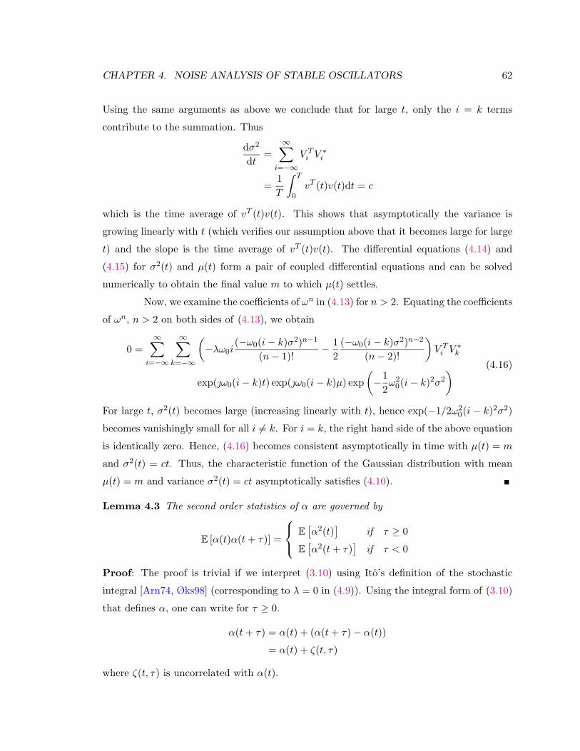
CHAPTER 4. NOISE ANALYSIS OF STABLE OSCILLATORS 62
Using the same arguments as above we conclude that for large t, only the i = k terms
contribute to the summation. Thus
dσ2
dt=
∞∑i=−∞
V Ti V
∗i
=1T
∫ T
0vT (t)v(t)dt = c
which is the time average of vT (t)v(t). This shows that asymptotically the variance is
growing linearly with t (which verifies our assumption above that it becomes large for large
t) and the slope is the time average of vT (t)v(t). The differential equations (4.14) and
(4.15) for σ2(t) and µ(t) form a pair of coupled differential equations and can be solved
numerically to obtain the final value m to which µ(t) settles.
Now, we examine the coefficients of ωn in (4.13) for n > 2. Equating the coefficients
of ωn, n > 2 on both sides of (4.13), we obtain
0 =∞∑
i=−∞
∞∑k=−∞
(−λω0i
(−ω0(i− k)σ2)n−1
(n− 1)!− 1
2(−ω0(i− k)σ2)n−2
(n− 2)!
)V Ti V
∗k
exp(ω0(i− k)t) exp(ω0(i− k)µ) exp(−1
2ω2
0(i− k)2σ2
) (4.16)
For large t, σ2(t) becomes large (increasing linearly with t), hence exp(−1/2ω20(i − k)2σ2)
becomes vanishingly small for all i 6= k. For i = k, the right hand side of the above equation
is identically zero. Hence, (4.16) becomes consistent asymptotically in time with µ(t) = m
and σ2(t) = ct. Thus, the characteristic function of the Gaussian distribution with mean
µ(t) = m and variance σ2(t) = ct asymptotically satisfies (4.10).
Lemma 4.3 The second order statistics of α are governed by
E [α(t)α(t+ τ)] =
E
[α2(t)
]if τ ≥ 0
E
[α2(t+ τ)
]if τ < 0
Proof: The proof is trivial if we interpret (3.10) using Ito’s definition of the stochastic
integral [Arn74, Øks98] (corresponding to λ = 0 in (4.9)). Using the integral form of (3.10)
that defines α, one can write for τ ≥ 0.
α(t+ τ) = α(t) + (α(t+ τ)− α(t))
= α(t) + ζ(t, τ)
where ζ(t, τ) is uncorrelated with α(t).

CHAPTER 4. NOISE ANALYSIS OF STABLE OSCILLATORS 63
For general λ we observe that given τ ≥ 0,
E [α(t)α(t+ τ)] = E
[∫ t
0
∫ t+τ
0vT (t1 + α(t1))ξ(t1)vT (t2 + α(t2))ξ(t2)dt2dt1
]= E
[∫ t
0
∫ t
0vT (t1 + α(t1))ξ(t1)vT (t2 + α(t2))ξ(t2)dt1dt2
]+ E
[∫ t
0
∫ t+τ
tvT (t1 + α(t1))v(t2 + α(t2))ξT (t1)ξ(t2)dt2dt1
]= E
[α2(t)
]+ E
[∫ t
0
∫ t+τ
tvT (t1 + α(t1))v(t2 + α(t2))ξT (t1)ξ(t2)dt2dt1
]= E
[α2(t)
]+∫ t
0
∫ t+τ
tE
[vT (t1 + α(t1))v(t2 + α(t2))ξT (t1)ξ(t2)
]dt2dt1
(4.17)
We define r12 = vT (t1 + α(t1))v(t2 + α(t2)) as a random process which is correlated with
both ξ(t1) and ξ(t2). However, v is periodic in it’s argument hence we can find a scalar M
such that −M ≤ r12 ≤ M . We use this fact to bound the above expectation. We define
pR12,Ξ1,Ξ2(r12, ξ1, ξ2) as the joint probability density function of the three random variables
r12, ξ1 , ξ(t1) and ξ2 , ξ(t2). Using this we obtain
E
[r12ξ
T1 ξ2
]=∫∫∫
r12ξT1 ξ2pR12,Ξ1,Ξ2(r12, ξ1, ξ2)dr12dξ1dξ2
Since −M ≤ r12 ≤M , we have
−M∫∫∫
ξT1 ξ2pR12,Ξ1,Ξ2(r12, ξ1, ξ2)dr12dξ1dξ2 ≤ E[r12ξ
T1 ξ2
]≤
M
∫∫∫ξT1 ξ2pR12,Ξ1,Ξ2(r12, ξ1, ξ2)dr12dξ1dξ2
or
−M∫∫
ξT1 ξ2pΞ1,Ξ2(ξ1, ξ2)dξ1dξ2 ≤ E[r12ξ
T1 ξ2
]≤
M
∫∫ξT1 ξ2pΞ1,Ξ2(ξ1, ξ2)dξ1dξ2
or
−Mnδ(t1 − t2) ≤∫∫∫
r12ξT1 ξ2pR12,Ξ1,Ξ2(r12, ξ1, ξ2)dr12dξ1dξ2 ≤Mnδ(t1 − t2)
where n is the size of ξ(t1) and ξ(t2). Hence
−Mn
∫ t
0
∫ t+τ
tδ(t1 − t2)dt2dt1 ≤
∫ t
0
∫ t+τ
tE
[vT (t1 + α(t1))v(t2 + α(t2))ξT (t1)ξ(t2)
]dt2dt1
≤Mn
∫ t
0
∫ t+τ
tδ(t1 − t2)dt2dt1
CHAPTER 4. NOISE ANALYSIS OF STABLE OSCILLATORS 64
Evaluation of the above integrals also depends on the particular definition of δ function
being used. Let us define f1(t) as a rectangular box of height 1/ε between [−λε, (1 − λ)ε]
and zero elsewhere. For any 0 ≤ λ ≤ 1, as ε → 0, f1(t) → δ(t). We evaluate the above
integral using this f1(t) and later take the limit ε→ 0. In the above integral, t2 varies from
t to t+ τ and t1 varies from 0 to t.∫ t
0
∫ t+τ
tδ(t1 − t2)dt2dt1 = lim
ε→0
∫ t
0
∫ t+τ
tf1(t1 − t2)dt2dt1
= limε→0
∫ t
0f2(t1)dt1
Where
f1(t2) =
0 t2 < −λε1ε −λε ≤ t2 ≤ (1− λ)ε
0 t2 > (1− λ)ε
and
f2(t1) =
0 t1 ≤ t− ε(1− λ)t1−t+ε(1−λ)
ε t− ε(1− λ) ≤ t1 ≤ t+ λε
1 t+ λε ≤ t1 ≤ t+ τ − ε(1− λ)t+τ−t1−ελ
ε t+ τ − ε(1− λ) ≤ t1 ≤ t+ τ + λε
0 t+ τ + λε ≤ t1
Therefore ∫ t
0
∫ t+τ
tδ(t1 − t2)dt2dt1 = lim
ε→0
∫ t
0f2(t1)dt1
= limε→0
12ε(1− λ)2
= 0
Hence the second integral in (4.17) is identically zero and E [α(t)α(t+ τ)] = E
[α2(t)
].
Corollary 4.4 Asymptotically with t
E [α(t)α(t+ τ)] = m2 + cmin(t, t+ τ)
Proof: Follows trivially from Lemma 4.3
Definition 4.1 Two real valued random variables Ψ1 and Ψ2 are called jointly Gaussian
if for all a1, a2 ∈ R, the real random variable a1Ψ1 + a2Ψ2 is Gaussian.

CHAPTER 4. NOISE ANALYSIS OF STABLE OSCILLATORS 65
Theorem 4.5 Asymptotically with time, α(t1) and α(t2) become jointly Gaussian.
Sketch of Proof: The proof is trivial if we interpret (3.10) using Ito’s definition of the
stochastic integral [Arn74] (corresponding to λ = 0 in (4.9)), as in the proof of Lemma 4.3.
The proof is more involved for 0 < λ ≤ 1. In this case, we prove this result by showing
that the cumulants of a1α(t1) + a2α(t2) (for any a1, a2 ∈ R) vanish for order higher than 2.
The cumulants of a random variable Ψ are defined as the coefficients in the Taylor series
expansion of its cumulant generating function which is, in turn, defined by
Kψ = logE [exp (θΨ)] =∞∑i=1
1i!ki(Ψ)θi
where ki(Ψ) is the ith order cumulant [GS92]. A random variable is Gaussian if and only if
its cumulants of order higher than 2 vanish [Gar83]. In the proof, we also use the fact that
α(t1) and α(t2) become individually Gaussian asymptotically with t.
The stochastic characterization of the phase deviation α that we obtained in this
section can be summarized by Lemma 4.3, Corollary 4.4 and Theorem 4.5. These do
not completely specify the FDDs of α as a stochastic process. However, they provide
adequate information for a practical characterization of the effect of phase deviation α on
the signal generated by an autonomous oscillator, e.g., its spectral properties, as we will see
in Section 4.2 and Section 4.3.
4.2 Spectrum of Oscillator Output with Phase Noise
Having obtained the asymptotic stochastic characterization of α, we now compute
the power spectral density (PSD) of xs(t+α(t)) where xs(t) is the steady-state response of
(3.1). We first obtain an expression for the nonstationary autocorrelation function R(t, τ)
of xs(t + α(t)). Next, we demonstrate that the autocorrelation becomes independent of
t asymptotically. This implies our main result, that the autocorrelation of the oscillator
output with phase noise contains no nontrivial cyclostationary components. This confirms
the intuitive expectation that a noisy autonomous system cannot have periodic cyclosta-
tionary variations because it has no perfect time reference. Finally, we show that the PSD
of the stationary component is a summation of Lorentzian spectra, and that a single scalar
constant, namely c in (4.12), is sufficient to characterize it.

CHAPTER 4. NOISE ANALYSIS OF STABLE OSCILLATORS 66
We start by calculating the autocorrelation function of xs(t+ α(t)), given by
R(t, τ) = E [xs(t+ α(t))x∗s(t+ τ + α(t+ τ))] (4.18)
Definition 4.2 Let Xi to be the Fourier coefficients of xs(t):
xs(t) =∞∑
i=−∞Xi exp (iω0t)
The following simple Lemma establishes the basic form of the autocorrelation:
Lemma 4.6 The autocorrelation of the oscillator output xs(t+ α(t)) is given by
R(t, τ) =∞∑
i=−∞
∞∑k=−∞
XiX∗k exp ((i− k)ω0t) exp (−kω0τ)E [exp (ω0βik(t, τ))] (4.19)
where
βik(t, τ) = iα(t)− kα(t+ τ)
and ω0 = 1/T .
Proof: Follows directly from (4.18) and Definition 4.2.
To evaluate the expectation in the above Lemma, it is useful to first consider the
statistics of βik(t, τ).
Lemma 4.7 The statistics of βi,k(t, τ) satisfy the following equations:
limt→∞
E [βik(t, τ)] = (i− k)m (4.20)
limt→∞
E
[(βik(t, τ))2
]− (E [βik(t, τ)])2 = (i− k)2ct+ k2cτ − 2ikcmin(0, τ) (4.21)
where m and c are defined in Theorem 4.2. Also, βik(t, τ) becomes Gaussian asymptotically
with t.
Proof: From Theorem 4.2 we observe that
limt→∞
E [βik(t, τ)] = i limt→∞
E [α(t)]− k limt→∞
E [α(t+ τ)] = (i− k)m

CHAPTER 4. NOISE ANALYSIS OF STABLE OSCILLATORS 67
Using Corollary 4.4 we have
limt→∞
E
[β2ik(t, τ)
]= i2 lim
t→∞E
[α2(t)
]+ k2 lim
t→∞E
[α2(t+ τ)
]− 2ik lim
t→∞E [α(t)α(t+ τ)]
= i2(m2 + ct) + k2(m2 + c(t+ τ))− 2ik(m2 + cmin(t, t+ τ))
= (i− k)2(m2 + ct) + k2cτ − 2ikcmin(0, τ)
This implies that
limt→∞
E
[(βik(t, τ))2
]− (E [βik(t, τ)])2 = (i− k)2ct+ k2cτ − 2ikcmin(0, τ)
The fact that βik(t, τ) is asymptotically Gaussian follows directly from Theo-
rem 4.5.
Using the asymptotically Gaussian nature of βik(t, τ), we are now able to obtain
a form for the expectation in (4.19).
Lemma 4.8 If c > 0, the characteristic function of βik(t, τ) is asymptotically independent
of t and has the following form:
limt→∞
E [exp (ω0βik(t, τ))] =
0 if i 6= k
exp (−12ω
20k
2c|τ |) if i = k(4.22)
Proof: Using Lemma 4.7 and the form of the characteristic function of a Gaussian random
variable [GS92] we have
limt→∞
E [exp (ω0βik(t, τ))] = exp(ω0(i− k)m)
exp(−1
2ω2
0((i− k)2ct+ k2cτ − 2ikcmin(0, τ)))
Taking the asymptotic limit of this expression, we observe that only for i = k the above
limit has a nontrivial value.
Using the second order statistics of βi,k(t, τ) we can now obtain the second order
statistics of xs(t+ α(t)) as follows:
Lemma 4.9 The autocorrelation R(t, τ) given by (4.19) satisfies
limt→∞
R(t, τ) =∞∑
i=−∞XiX
∗i exp (−iω0τ) exp
(−1
2ω2
0i2c|τ |
)(4.23)
Proof: The result is obtained by substituting (4.22) in (4.19).
The spectrum of xs(t+ α(t)) can now be determined as follows:

CHAPTER 4. NOISE ANALYSIS OF STABLE OSCILLATORS 68
Theorem 4.10 The spectrum of xs(t+α(t)) is determined by the asymptotic behaviour of
R(t, τ) as t→∞. All nontrivial cyclostationary components are zero, while the stationary
component of the spectrum is given by:
S(ω) =∞∑
i=−∞XiX
∗i
ω20i
2c14ω
40i
4c2 + (ω + iω0)2(4.24)
There is also a term X0X∗0 δ(ω) due to the DC part of xs(t), which is omitted in (4.24).
Proof: It can be shown that the cyclostationary component [Gar90] of the autocorrelation
at any frequency ωcyc is given by:
Rωcyc(τ) = limT→∞
1T
∫ T
0R(t, τ) exp (ωcyct) dt
This expression is determined by the asymptotic form of R(t, τ) as a function of t, given
in (4.23). Because this becomes independent of t, the above limit is identically zero for all
ωcyc 6= 0, whereas for ωcyc = 0 (the stationary component), it reduces to (4.23). The result
is obtained by taking the Fourier transform of (4.23).
Hence we conclude that the output of a noisy oscillator xs(t + α(t)) is a large
stochastic process which is wide-sense stationary. The power spectral density of the output
consists of a series of Lorentzians centered around the harmonics of the oscillator.
These results have important implications. The noisy oscillator output cannot be
viewed as a deterministic periodic signal along with additive noise. We conclude that it
should be viewed as a sum of two stochastic processes: a large signal output process with
stochastic phase error which behaves like Brownian motion and a small amplitude noise
process. Among other implications, this requires us to revisit the noise analysis techniques
for nonautonomous circuits which we motivate and present in the next two chapters.
The Lorentzian shape of the output spectrum implies that the power spectral
density at the carrier frequency and its harmonics has a finite value. Integrating the power
spectral density we observe that∫ ∞−∞
S(ω)dω =∫ ∞−∞
∞∑i=−∞
XiX∗i
ω20i
2c14ω
40i
4c2 + (ω + iω0)2dω
=∞∑
i=−∞XiX
∗i
i.e., the total carrier power is preserved despite spectral spreading due to noise. This
result is physically consistent since adding a stochastic phase error α(t) to the oscillator
CHAPTER 4. NOISE ANALYSIS OF STABLE OSCILLATORS 69
−1 −0.8 −0.6 −0.4 −0.2 0 0.2 0.4 0.6 0.8 1
x 109
10−18
10−16
10−14
10−12
10−10
10−8
10−6
10−4
10−2
100
Power Spectral Density of Phase Noise Process (w0=1e8,c=1e−15)
Angular Frequency (radian/sec)
Noi
se P
SD
Figure 4.1: Power spectral density of noisy oscillator output
steady-state response should not change the total integrated power. Previous analyses based
on linear time-invariant (LTI) or linear time-varying (LTV) concepts erroneously predict
infinite noise power density at the carrier, as well as infinite total integrated power. That
the oscillator output is stationary is surprising at first sight, since oscillators are nonlinear
systems with periodic swings, hence it might be expected that output noise power would
change periodically as in forced systems. However, it must be remembered that while forced
systems are supplied with an external time reference (through the forcing), oscillators are
not. Cyclostationarity in the oscillator’s output would, by definition, imply a perfect time
reference. Hence the stationarity result reflects the fundamental fact that noisy autonomous
systems cannot provide a perfect time reference.
The power spectral density as calculated in (4.24) is shown in Figure 4.1 for ω0 =
1×10⁸ rad/sec and c = 1×10⁻¹⁵ sec. It consists of peaks at the harmonics of the oscillator
which rapidly decay away from the harmonics. Figure 4.2 shows the power spectral density
as a function of offset frequency around the first harmonic. We observe that the PSD does

CHAPTER 4. NOISE ANALYSIS OF STABLE OSCILLATORS 70
10−2
100
102
104
106
10−12
10−10
10−8
10−6
10−4
10−2
100
Power Spectral Density of Phase Noise Process
Offset Angular Frequency (radian/sec)
Noi
se P
SD
Figure 4.2: Power spectral density around the first harmonic
not blow up to infinity at ∆ω → 0 but flattens out to a finite value.
4.3 Phase Noise Characterization for Oscillator
In this section, we discuss several popular characterizations of phase noise that are
used in the design of electronic oscillators, and how they can easily be obtained from the
stochastic characterization we obtained in Section 4.1 and Section 4.2.
4.3.1 Single-Sided Spectral Density and Total Power
The PSD S(ω) in (4.24) (defined for −∞ < ω < ∞, hence called a double-sided
density) is a real and even function of ω, because the periodic steady-state xs(t) is real
hence its Fourier series coefficients Xi in Definition 4.2 satisfy Xi = X∗−i. The single-sided
spectral density (defined for 0 ≤ f <∞) is given by
Sss(f) = 2S(2πf) = 2∞∑
i=−∞XiX
∗i
f20 i
2c
π2f40 i
4c2 + (f + if0)2(4.25)

CHAPTER 4. NOISE ANALYSIS OF STABLE OSCILLATORS 71
where we substituted ω = 2πf and ω0 = 2πf0. The total power (i.e., the integral of the
PSD over the range of the frequencies it is defined for) in Sss(f) is the same as in S(2πf),
which is
Ptot = Total power in Sss(f) =∫ ∞
0Sss(f)df =
∞∑i=1
2 |Xi|2 (4.26)
The total power in the periodic signal xs(t) (without phase noise) is also equal to the
expression in (4.26) (excluding the power in the DC part), as can be easily seen from the
Fourier expansion in Definition 4.2.
The phase deviation α(t) does not change the total power in the periodic signal
xs(t), but it alters the power density in frequency, i.e., the power spectral density. For the
perfect periodic signal xs(t), the power spectral density has δ functions located at discrete
frequencies (i.e., the harmonics). The phase deviation α(t) spreads the power in these δ
functions in the form given in (4.25), which can be experimentally observed with a spectrum
analyzer.
4.3.2 Spectrum in dBm/Hz
For electrical oscillators, the state variable in the oscillator that is observed as the
output is usually a voltage or a current. The spectrum in (4.25) is expressed as a function
of frequency (f in Hz), then the PSD is in units of volts2/Hz and amps2/Hz for a voltage
and a current state variable respectively. Then, the spectral density of the expected power
dissipated in a 1Ω resistor (with the voltage (current) output of the oscillator as the voltage
across (current through) the resistor) is equal to the PSD in (4.25) (in watts/Hz), which is
usually expressed in dBw/Hz as defined by
SdBw(f) = 10 log10 (Sss(f) in watts/Hz) (4.27)
This expected power is the same as the time-average power, assuming that the stochastic
process xs(t+α(t)) is ergodic [Gar90]. If Sss(f) is in miliwatts/Hz, then the PSD in dBm/Hz
is given by
SdBm(f) = 10 log10 (Sss(f) miliwatts/Hz) (4.28)
4.3.3 Single-Sideband Phase Noise Spectrum in dBc/Hz
In practice, we are usually interested in the PSD around the first harmonic, i.e.,
Sss(f) for f around f0. The single-sideband phase noise L(fm) (in dBc/Hz) that is very

CHAPTER 4. NOISE ANALYSIS OF STABLE OSCILLATORS 72
widely used in practice is defined as
L(fm) = 10 log10
(Sss(fo + fm)
2|X1|2
)(4.29)
For “small” values of c, and for 0 ≤ fm f0, (4.29) can be approximated as
L(fm) ≈ 10 log10
(f2
0 c
π2f40 c
2 + f2m
)(4.30)
Furthermore, for πf20 c fm f0, L(fm) can be approximated by
L(fm) ≈ 10 log10
((f0
fm
)2
c
)(4.31)
Notice that the approximation of L(fm) in (4.31) blows up as fm → 0. For 0 ≤ fm < πf20 c,
(4.31) is not accurate, in which case the approximation in (4.30) should be used.
4.3.4 Timing Jitter
In some applications, such as clock generation and recovery, one is interested
in a characterization of the phase/time deviation α(t) itself rather than the spectrum of
xs(t+α(t)) that was calculated in Section 4.2. In these applications, an oscillator generates
a square-wave like waveform to be used as a clock. The effect of the phase deviation α(t)
on such a waveform is to create uncertainty jitter in the zero-crossing or transition times.
In Section 4.1, we found out that α(t) (for an autonomous oscillator) becomes a Gaussian
random variable with a linearly increasing variance
σ2(t) = ct
Let us take one of the transitions (i.e., edges) of a clock signal as a reference (i.e., trigger)
transition and synchronize it with t = 0. If the clock signal is perfectly periodic, then one
will see transitions exactly at tk = kT , k = 1, 2, . . . where T is the period. For a clock signal
with a phase deviation α(t) that has a linearly increasing variance as above, the timing of
the kth transition tk will have a variance (i.e., mean-square error)
E
[(tk − kT )2
]= ckT (4.32)
The spectral dispersion caused by α(t) in an oscillation signal can be observed with a
spectrum analyzer. Similarly, one can observe the timing jitter caused by α(t) using a

CHAPTER 4. NOISE ANALYSIS OF STABLE OSCILLATORS 73
sampling oscilloscope. McNeill [McN97] experimentally observed the linearly increasing
variance for the timing of the transitions of a clock signal generated by an autonomous
oscillator, as predicted by our theory. Moreover, c (in sec2Hz) in (4.32) exactly quantifies
the rate of increase of timing jitter with respect to a reference transition. Another useful
figure of merit is the cycle-to-cycle timing jitter, i.e., the timing jitter in one clock cycle,
which has a variance cT .
4.4 Noise Source Contribution
The scalar constant c appears in all of the characterizations we discussed above.
It is given by
c =1T
∫ T
0vT1 (τ)D(xs(τ))DT (xs(τ))v1(τ)dτ (4.33)
where D(·) : Rn → Rn×p represents the modulation of the intensities of the noise sources
with the large-signal state. (4.33) can be rewritten as
c =p∑i=1
1T
∫ T
0[vT1 (τ)Di(τ)]2 dτ =
p∑i=1
ci
where p is the number of the noise sources, i.e., the column dimension of D(xs(·)), and
Di(·) is the ith column of D(xs(·)) which maps the ith noise source to the equations of the
system. Hence,
ci =1T
∫ T
0[vT1 (τ)Di(τ)]2dτ
represents the contribution of the ith noise source to c. Thus, the ratio
cic =
∑pi=1 ci
(4.34)
can be used as a figure of merit representing the contribution of the ith noise source to
phase noise/timing jitter.
One can also define
c(k)s =
1T
∫ T
0[vT1 (τ) ek]2dτ (4.35)
(where 1 ≤ k ≤ n and ek is the kth unit vector) as the phase noise/timing jitter sensitivity
of the kth equation (i.e., node), because ek represents a unit intensity noise source added to
the kth equation (i.e., connected to the kth node) in (3.1).

CHAPTER 4. NOISE ANALYSIS OF STABLE OSCILLATORS 74
4.5 Numerical Techniques for Phase Noise Characterization
From Section 4.1, Section 4.2 and Section 4.3 we observe that for various phase
noise characterizations of an oscillator, one needs to calculate the steady-state periodic
solution xs(t), and the periodic vector v1(t) in (4.33). xs(t) is available from the steady-
state analysis of the circuit. We outline two methods, one in time domain and one in
frequency domain, for computing the periodic vector v1(t).
4.5.1 Time Domain Technique
The procedure for calculating v1(t) in the time domain is as follows:
1. The large signal periodic steady-state solution xs(t) is computed for 0 ≤ t ≤ T by
numerically integrating (3.1), either using transient simulation or possibly using a
technique such as the shooting method [KWSV90] to directly compute the steady-
state response of the oscillator.
2. The state transition matrix Φ(T, 0) is computed (see Section 3.2.1) by numerically
integrating
Y = J(t)Y Y (0) = In
from 0 to T , where the Jacobian J(t) is defined in (3.3). We recall that
Φ(T, 0) = Y (T )
3. u1(0) is computed using
u1(0) = xs(0)
u1(0) is an eigenvector of Φ(T, 0) corresponding to the eigenvalue 1.
4. v1(0) is an eigenvector of ΦT (T, 0) corresponding to the eigenvalue 1. To compute
v1(0), first compute an eigenvector of ΦT (T, 0) corresponding to the eigenvalue 1,
then scale this eigenvector so that
v1(0)Tu1(0) = 1 (4.36)
is satisfied.

CHAPTER 4. NOISE ANALYSIS OF STABLE OSCILLATORS 75
5. The periodic vector v1(t) is computed for 0 ≤ t ≤ T by numerically solving the adjoint
system
y = −JT (t)y (4.37)
using v1(0) = v1(T ) as the initial condition. v1(t) is a periodic steady-state solution of
(4.37) corresponding to the Floquet exponent that is equal to 0, i.e., µ1 = 0. Since J
is the Jacobian of an asymptotically orbitally stable oscillator, it is not possible to cal-
culate v1(t) by numerically integrating (4.37) forward in time, because the numerical
errors in computing the solution and the numerical errors in the initial condition v1(0)
will excite the modes of the solution of (4.37) that grow without bound. However,
one can integrate (4.37) backwards in time with the “initial” condition v1(T ) = v1(0)
to calculate v1(t) for 0 ≤ t ≤ T in a numerically stable way.
6. Then, c is calculated using (4.33).
We implemented the above algorithm partly in Spice and partly in Matlab.
Transient simulation of the oscillator circuit is performed in Spice till steady-state is
reached. The circuit is then simulated for one period with very small time step. The
circuit matrices that are generated during this step are handed over to Matlab where
noise analysis is performed. In implementing the above algorithm, one can increase the
efficiency by saving LU factored matrices that needs to be calculated in Step 2 and reuse
them in Step 5. If the periodic steady-state xs(t) of the oscillator is calculated using the
shooting method [KWSV90] in Step 1, then the state transition matrix Φ(T, 0) of the lin-
ear time varying system, obtained by linearizing the nonlinear oscillator circuit around the
periodic steady-state, is already available. It can be shown that the Jacobian of the non-
linear system of equations that is solved in the shooting method, using Newton’s method
to calculate the initial condition that results in the periodic steady-state solution, is equal
to Φ(T, 0)− I [AT72a, AT72b].
Moreover, one can avoid calculating Φ(T, 0) explicitly, and use iterative methods
both for the shooting method, and at Step 4 to calculate the eigenvector of ΦT (T, 0) that
corresponds to the eigenvalue 1. For high-Q oscillators, the iterative methods can run into
problems, because Φ(T, 0) may have several other eigenvalues which are close to 1. In our
implementation, we explicitly calculate Φ(T, 0) and perform a full eigenvalue/eigenvector
calculation. We select all the eigenvectors corresponding the eigenvalues which are close to
CHAPTER 4. NOISE ANALYSIS OF STABLE OSCILLATORS 76
1 and use the following relation to determine the correct eigenvalue
vi(0)Tu1(0) = vi(0)xs(0)
=
1 i = 1
0 i 6= 1
We first calculate xs(t) from the steady-state response of the oscillator. We then calcu-
late the inner product with vi(0)’s whose corresponding eigenvalues are close to 1. Due
to numerical errors in determining the period and integration, the inner product is not
exactly zero but the desired eigenvalue is easily identified. Full eigenvector/eigenvalue de-
composition also allows us to investigate the properties of the state transition matrix for
various oscillator circuits. Even with a full eigenvalue/eigenvector calculation for Φ(T, 0),
the phase noise characterization algorithm discussed above is still very efficient. The phase
noise characterization comes almost for free once the periodic steady-state solution xs(t) is
computed.
4.5.2 Frequency Domain Technique
Here we outline how we can calculate v1(t) using a frequency domain technique
such as harmonic balance. We consider (3.4)
w = J(t)w
This describes a linear periodic time varying system of equation and represents an LPTV
transfer function h(t, s) = Φ(t, s) where Φ(t, s) is the state transition matrix of w = Jw.
h(t, s) is periodic in both it’s arguments with period T , i.e.,
h(t+ T, s+ T ) = h(t, s)
The periodicity of h implies that it can be expanded in a Fourier series [RFL98]
h(t, s) =∞∑
i=−∞hi(t− s) exp(iω0t) ω0 =
2πT
(4.38)
hi are referred to as harmonic impulse response of the LPTV system. The Fourier transform
of hi, Hi(ω) is defined as
Hi(ω) =∫ ∞−∞
hi(t) exp(−ωt)dt (4.39)
A harmonic balance technique for solving x = f(x) typically yields a harmonic balance
conversion matrix which is defined as follows.

CHAPTER 4. NOISE ANALYSIS OF STABLE OSCILLATORS 77
Definition 4.3 ([RFL98]) The harmonic balance conversion matrix is defined in terms
of His as
H(ω) =
......
......
...
· · · H0(ω + 2ω0) H1(ω + ω0) H2(ω) H3(ω − ω0) H4(ω − 2ω0) · · ·· · · H−1(ω + 2ω0) H0(ω + ω0) H1(ω) H2(ω − ω0) H3(ω − 2ω0) · · ·· · · H−2(ω + 2ω0) H−1(ω + ω0) H0(ω) H1(ω − ω0) H2(ω − 2ω0) · · ·· · · H−3(ω + 2ω0) H−2(ω + ω0) H−1(ω) H0(ω − ω0) H1(ω − 2ω0) · · ·· · · H−4(ω + 2ω0) H−3(ω + ω0) H−2(ω) H−1(ω − ω0) H0(ω − 2ω0) · · ·
......
......
...
Definition 4.4 We define the matrices Ui and Vi to be the Fourier components of U(t)
and V (t), i.e.,
U(t) =∞∑
i=−∞Uie
ω0it (4.40)
V (t) =∞∑
i=−∞Vie
ω0it (4.41)
Definition 4.5 We define the block-Toeplitz matrices U and V as follows:
U =
. . .
U0 U1 U2 . . . . . .
U−1 U0 U1 U2 . . .
U−2 U−1 U0 U1 U2
. . . U−2 U−1 U0 U1
. . . . . . U−2 U−1 U0
. . .
(4.42)
V =
. . .
V0 V1 V2 . . . . . .
V−1 V0 V1 V2 . . .
V−2 V−1 V0 V1 V2
. . . V−2 V−1 V0 V1
. . . . . . V−2 V−1 V0
. . .
(4.43)
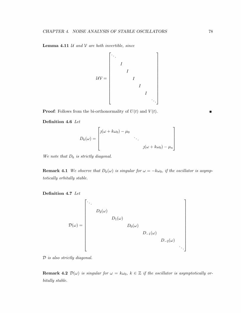
CHAPTER 4. NOISE ANALYSIS OF STABLE OSCILLATORS 78
Lemma 4.11 U and V are both invertible, since
UV =
. . .
I
I
I
I
I
. . .
Proof: Follows from the bi-orthonormality of U(t) and V (t).
Definition 4.6 Let
Dk(ω) =
(ω + kω0)− µ0
. . .
(ω + kω0)− µn
We note that Dk is strictly diagonal.
Remark 4.1 We observe that Dk(ω) is singular for ω = −kω0, if the oscillator is asymp-
totically orbitally stable.
Definition 4.7 Let
D(ω) =
. . .
D2(ω)
D1(ω)
D0(ω)
D−1(ω)
D−2(ω). . .
D is also strictly diagonal.
Remark 4.2 D(ω) is singular for ω = kω0, k ∈ Z if the oscillator is asymptotically or-
bitally stable.

CHAPTER 4. NOISE ANALYSIS OF STABLE OSCILLATORS 79
Theorem 4.12 The frequency-domain conversion matrix H(ω) of the oscillator is related
to U , D(ω) and V by:
H(ω) = UD−1(ω)V
Proof: We know that the transfer function h(t, s) is the state transition matrix Φ(t, s).
Hence for τ > 0
Φ(t, t− τ) = U(t) exp(Dτ)V (t− τ)
=∞∑
k=−∞
∞∑l=−∞
Uk exp(Dτ)Vl exp(ω0(kt+ lt− lτ))
The coefficient of exp(ω0it) in the above expression is given by
hi(τ) =∞∑
k=−∞Uk exp(Dτ)Vi−k exp(−ω0(i− k)τ)
and hence
Hi(ω) =∫ ∞−∞
∞∑k=−∞
Uk exp(Dτ)Vi−k exp(−ω0(i− k)τ) exp(ωτ)dτ
= −∞∑
k=−∞Uk[D − (ω0(i− k)− ω)I]−1Vi−k
where we have used the fact that φ(t, t − τ) is defined for τ ≥ 0 only. The result follows
immediately from the above form of Hi(ω).
Theorem 4.13 H−1(0) is a singular matrix (with rank-deficiency one) and the null space
of its transpose is spanned by the Fourier components of v1(t), i.e.,
ker(H−T (0)
)=[1 0 · · · 0
] [· · · V−2 V−1 V0 V1 V2 · · ·
]=[· · · V T
1,−2 V T1,−1 V T
1,0 V T1,1 V T
1,2 · · ·]
where V1,i are the Fourier coefficients of k vT1 (t), for some nonzero scalar k, i.e.,
kvT1 (t) =∞∑
i=−∞V T
1,i eω0it
Sketch of Proof: The proof follows from the fact that v1(t) is the eigenvector of ΦT (t, 0)
corresponding to eigenvalue 1.
H−T (0) is simply the transpose of the Harmonic Balance Jacobian matrix of the
oscillator at solution. Its null space can be found efficiently even for large circuits by using

CHAPTER 4. NOISE ANALYSIS OF STABLE OSCILLATORS 80
−+
−+
−+
QR C
R
RNoiseSource
R
QR R
C
R
Output
Figure 4.3: Oscillator with a band-pass filter and a comparator
iterative linear algebra techniques [RFL98]. Hence a scaled version of vT1 (t) can be found
easily. The scaling constant k can be found by applying vT1 (t)u1(t) = 1, u1(t) having first
been obtained by differentiating the large-signal steady-state solution of the oscillator.
4.6 Examples
We apply these characterization techniques to electrical oscillators. There are three
distinct kinds of electrical oscillators with three very different oscillation mechanisms. The
LC oscillator consists of a unstable feedback amplifier with frequency selection provided by
the LC tank circuit. A ring oscillator consists of a number of delay stages connected in
a ring. The frequency of oscillation is set by the number of stages and the delay of each
stage. A relaxation oscillator uses regenerative switching to produce the output waveform.
The signal generation mechanism for all these oscillators is very different but our analysis
is valid for all these oscillators.
4.6.1 Generic Oscillator
This oscillator (Figure 4.3) consists of a Tow-Thomas second-order bandpass filter
and a comparator [DTS98a]. If the OpAmps are considered to be ideal, it can be shown
that this oscillator is equivalent (in the sense of the differential equations that describe
it) to a parallel RLC circuit in parallel with a nonlinear voltage-controlled current source

CHAPTER 4. NOISE ANALYSIS OF STABLE OSCILLATORS 81
0.3 0.57 0.84 1.11 1.38 1.65 1.92 2.19 2.46 2.73 3
x 104
−80
−70
−60
−50
−40
−30
−20
−10
0
10
20
Frequency (Hz)Po
wer
Spe
ctra
l Den
sity
(dB
m)
(a) Computed PSD (4 harmonics)
(b) Spectrum analyzer measured PSD [DTS98a]
6300 6400 6500 6600 6700 6800 6900 7000−20
−15
−10
−5
0
5
10
15
Frequency (Hz)
Pow
er S
pect
ral D
ensi
ty (
dBm
)
(c) Computed PSD (first harmonic)
10−1
100
101
102
103
−60
−50
−40
−30
−20
−10
0
10
20
Frequency (Hz)
Sing
le-S
ideb
and
Phas
e N
oise
Spe
ctru
m (
dBc)
(d) L(fm) computed with (4.30) and (4.31)
0 0.5 1 1.5
x 10−4
0
0.5
1
1.5
2
2.5
3
3.5
4
4.5x 10
−7
Time (sec)
sec^
2. H
z
(e) (vT1 (t)D)2
Figure 4.4: Phase noise characterization for the generic oscillator
CHAPTER 4. NOISE ANALYSIS OF STABLE OSCILLATORS 82
(or equivalently a series RLC circuit in series with a nonlinear current-controlled voltage
source) as in Figure 4.3. In [DTS98a], authors bread-boarded this circuit with an external
white noise source (intensity of which was chosen such that its effect is much larger than
the other internal noise sources), and measured the PSD of the output with a spectrum
analyzer. For Q = 1 and fo = 6.66 KHz, we performed a phase noise characterization
of this oscillator using the numerical methods in Section 4.5, and computed the periodic
oscillation waveform xs(t) for the output and c = 7.56×10⁻⁸ sec2Hz. Figure 4.4(a) shows the
PSD of the oscillator output computed using (4.25), and Figure 4.4(b) shows the spectrum
analyzer measurement. Figure 4.4(c) shows an expanded version of the PSD around the
first harmonic. The single-sideband phase noise spectrum using both (4.30) and (4.31) is
in Figure 4.4(d). (4.31) can not predict the PSD accurately below the cut-off frequency
fc = πf20 c = 10.56 Hz (marked with a ∗ in Figure 4.4(d)) of the Lorentzian. The oscillator
model that was simulated has two state variables and a single stationary noise source.
Figure 4.4(e) shows a plot of the periodic nonnegative scalar
vT1 (t)D(xs(t))DT (xs(t))v1(t) = (vT1 (t)D)2
where D is independent of t since the noise source is stationary. c is the time average of
this scalar that is periodic in time.
4.6.2 LC Tank Oscillator
A Colpitt’s oscillator with an off-chip inductor is shown in Figure 4.5. This os-
cillator is designed to oscillate at 1.05 GHz. We computed c = 9.00 × 10⁻¹⁹ sec2Hz which
corresponds to L(fm) = −100 dBc/Hz at fm = 100 KHz using (4.31). The simplified cir-
cuit had 11 state variables and 8 noise sources. We generated a noise source contribution
report (Table 4.1) and found that 85% of the contribution to c is from the noise in base
spreading resistor rb of the transistor. A decrease in this value (due to sizing of transistor)
by a factor of 5 causes the value of c to be reduced to 4.38 × 10⁻¹⁹ sec2Hz. We also plot
vT1 (t)D(xs(t))DT (xs(t))v1(t) as a function of time for one period of oscillation(Figure 4.6).
We see that this value peaks at a time equal to half the period of oscillation. This also is
useful feedback to the designers as it can be used to further improve the noise performance
of this oscillator.
A simplified schematic of a 4.7 GHz oscillator with on-chip inductor is shown in
Figure 4.7 [Kin98]. This oscillator is fabricated in a standard digital 0.35 µ CMOS process

CHAPTER 4. NOISE ANALYSIS OF STABLE OSCILLATORS 83
RS
L RL C2
VCC
VEE
C1Q1
Figure 4.5: Colpitt’s Oscillator
0 0.2 0.4 0.6 0.8 1
x 10−9
0
2
4
6x 10
−18
Time (sec)
v 1T(t
)B(x
s(t))
BT(x
s(t))
v 1(t)
(sec
2 Hz)
Figure 4.6: vT1 (t)D(xs(t))DT (xs(t))v1(t) for the Colpitt’s oscillator
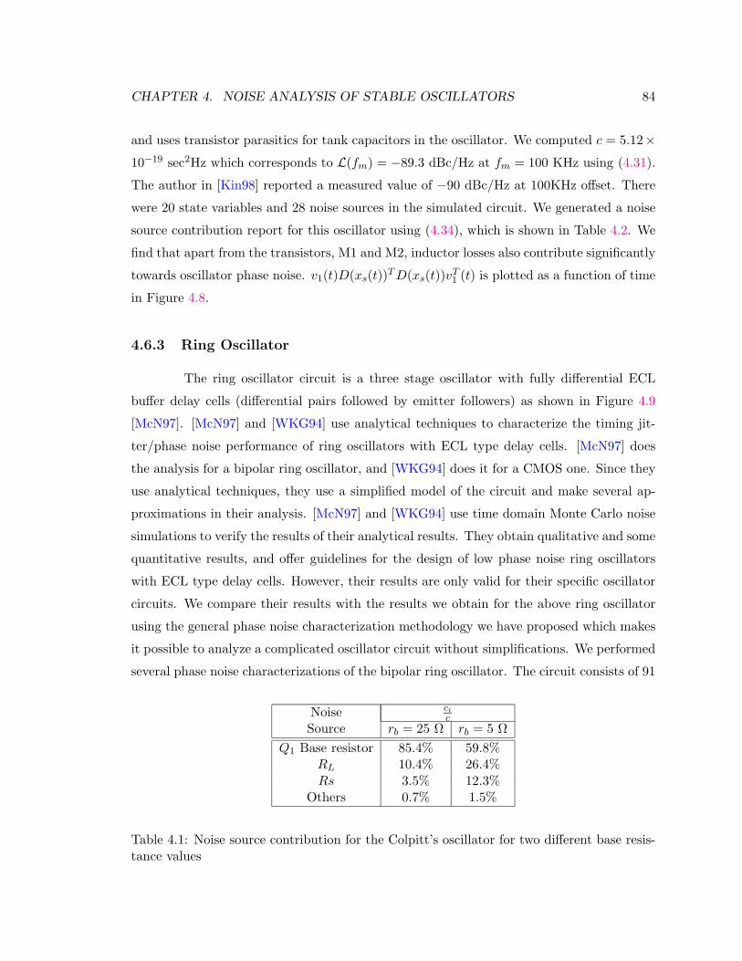
CHAPTER 4. NOISE ANALYSIS OF STABLE OSCILLATORS 84
and uses transistor parasitics for tank capacitors in the oscillator. We computed c = 5.12×10⁻¹⁹ sec2Hz which corresponds to L(fm) = −89.3 dBc/Hz at fm = 100 KHz using (4.31).
The author in [Kin98] reported a measured value of −90 dBc/Hz at 100KHz offset. There
were 20 state variables and 28 noise sources in the simulated circuit. We generated a noise
source contribution report for this oscillator using (4.34), which is shown in Table 4.2. We
find that apart from the transistors, M1 and M2, inductor losses also contribute significantly
towards oscillator phase noise. v1(t)D(xs(t))TD(xs(t))vT1 (t) is plotted as a function of time
in Figure 4.8.
4.6.3 Ring Oscillator
The ring oscillator circuit is a three stage oscillator with fully differential ECL
buffer delay cells (differential pairs followed by emitter followers) as shown in Figure 4.9
[McN97]. [McN97] and [WKG94] use analytical techniques to characterize the timing jit-
ter/phase noise performance of ring oscillators with ECL type delay cells. [McN97] does
the analysis for a bipolar ring oscillator, and [WKG94] does it for a CMOS one. Since they
use analytical techniques, they use a simplified model of the circuit and make several ap-
proximations in their analysis. [McN97] and [WKG94] use time domain Monte Carlo noise
simulations to verify the results of their analytical results. They obtain qualitative and some
quantitative results, and offer guidelines for the design of low phase noise ring oscillators
with ECL type delay cells. However, their results are only valid for their specific oscillator
circuits. We compare their results with the results we obtain for the above ring oscillator
using the general phase noise characterization methodology we have proposed which makes
it possible to analyze a complicated oscillator circuit without simplifications. We performed
several phase noise characterizations of the bipolar ring oscillator. The circuit consists of 91
Noise cic
Source rb = 25 Ω rb = 5 ΩQ1 Base resistor 85.4% 59.8%
RL 10.4% 26.4%Rs 3.5% 12.3%
Others 0.7% 1.5%
Table 4.1: Noise source contribution for the Colpitt’s oscillator for two different base resis-tance values

CHAPTER 4. NOISE ANALYSIS OF STABLE OSCILLATORS 85
R1ext
M1 M2
L1 L2
M5 M6
M3
C1ext
M4
2.7V3.3V
C2ext
L1ext L2ext R2ext
VTUNED1 D2
IBIAS
Figure 4.7: Oscillator with on-chip inductor
Noise sources of cic=∑pi=1 ci
× 100
M1 and M2 57.6 %Inductor losses 38.5 %
Others 3.9 %
Table 4.2: Noise Source Contribution for oscillator with on-chip inductor

CHAPTER 4. NOISE ANALYSIS OF STABLE OSCILLATORS 86
0 0.5 1 1.5 2 2.5
x 10−10
2
3
4
5
6
7
8x 10
−19
Time (sec)
v 1T(t
)B(x
s(t))
BT(x
s(t))
v 1(t)
(sec
2 Hz)
Figure 4.8: vT1 (t)D(xs(t))DT (xs(t))v1(t) for oscillator with on-chip inductor
state variables and 121 noise sources. The results are shown in Table 4.3, where Rc is the
collector load resistance for the differential pair (DP) in the delay cell, rb is the zero bias
base resistance for the BJTs in the DP, IEE is the tail bias current for the DP, and fo is
the oscillation frequency for the three stage ring oscillator. The changes in Rc and rb affect
the oscillation frequency, unlike the changes in IEE . Figure 4.10 shows a plot of (2πfo)2 c
versus IEE using the data from Table 4.3. This prediction of the dependence of phase
noise/timing jitter performance on the tail bias current is in agreement with the analysis
and experimental results presented in [McN97] and [WKG94] for ring oscillators with ECL
type delay cells. Larger values for (2πfo)2 c indicate worse phase noise performance.
4.6.4 Relaxation Oscillator
The relaxation oscillator is a VCO that is based on the emitter-coupled multi-
vibrator circuit [GM93]. [AM83] analyzes the process of jitter production for this circuit
by describing the circuit behaviour with a single first-order stochastic differential equation
based on a simplified model for the circuit, and lumping all of the noise sources into a
single stationary current noise source. [AM83] arrives at intuitive qualitative results for
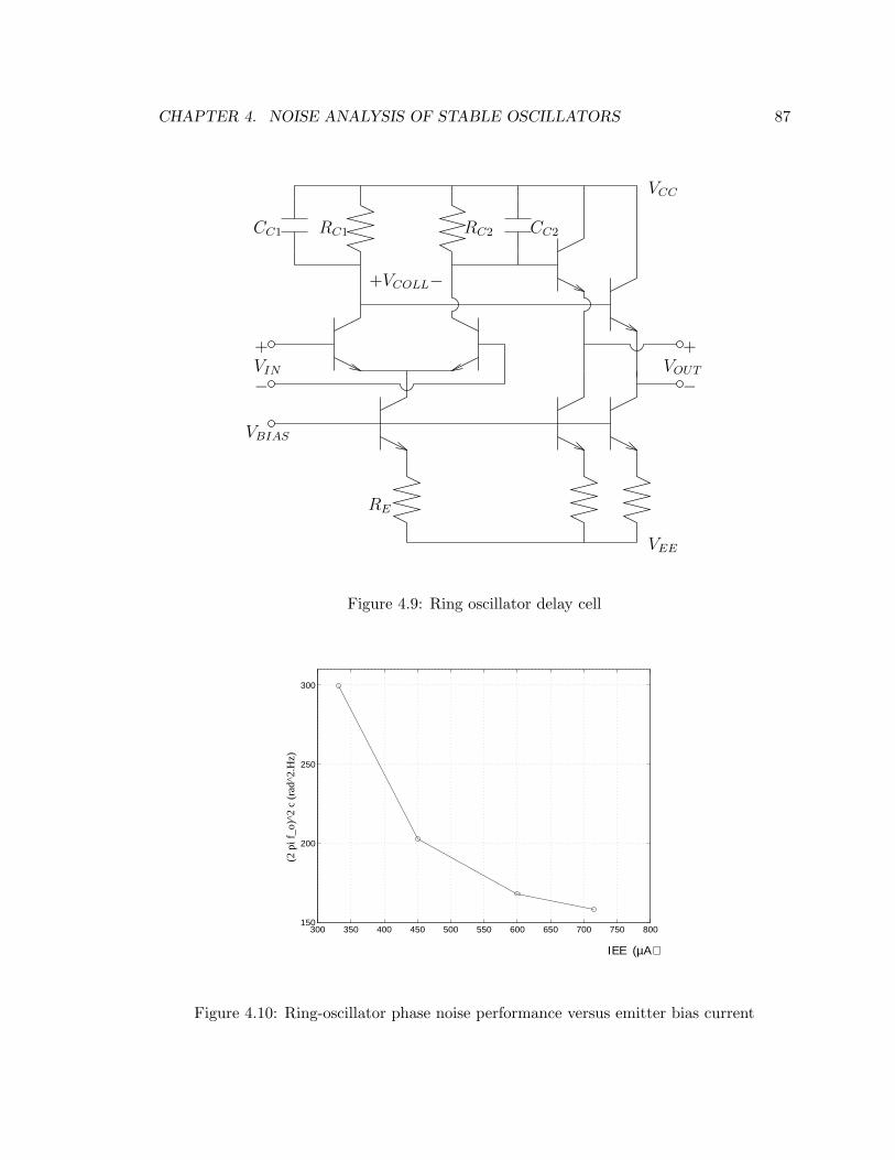
CHAPTER 4. NOISE ANALYSIS OF STABLE OSCILLATORS 87
VCC
VOUT
+
−
RC2 CC2
VEE
+VCOLL−
VIN
+
−
VBIAS
RE
RC1CC1
Figure 4.9: Ring oscillator delay cell
300 350 400 450 500 550 600 650 700 750 800150
200
250
300
ΙΕΕ (µΑ)
(2 p
i f_o
)^2
c (r
ad^2
.Hz)
Figure 4.10: Ring-oscillator phase noise performance versus emitter bias current
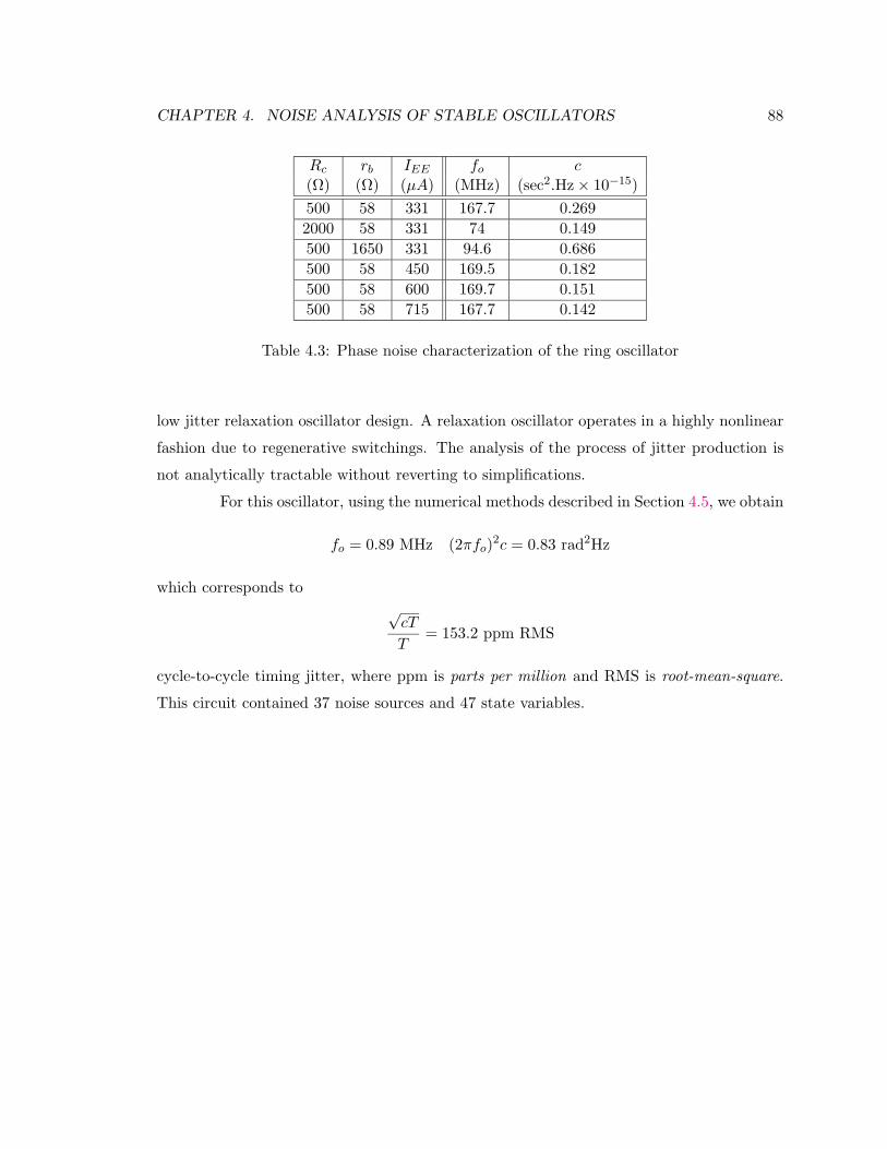
CHAPTER 4. NOISE ANALYSIS OF STABLE OSCILLATORS 88
Rc rb IEE fo c(Ω) (Ω) (µA) (MHz) (sec2.Hz× 10−15)500 58 331 167.7 0.2692000 58 331 74 0.149500 1650 331 94.6 0.686500 58 450 169.5 0.182500 58 600 169.7 0.151500 58 715 167.7 0.142
Table 4.3: Phase noise characterization of the ring oscillator
low jitter relaxation oscillator design. A relaxation oscillator operates in a highly nonlinear
fashion due to regenerative switchings. The analysis of the process of jitter production is
not analytically tractable without reverting to simplifications.
For this oscillator, using the numerical methods described in Section 4.5, we obtain
fo = 0.89 MHz (2πfo)2c = 0.83 rad2Hz
which corresponds to√cT
T= 153.2 ppm RMS
cycle-to-cycle timing jitter, where ppm is parts per million and RMS is root-mean-square.
This circuit contained 37 noise sources and 47 state variables.

89
Chapter 5
Noise Analysis of Nonautonomous
Circuits
In the previous chapter we developed a noise simulation and characterization
technique for oscillators. We found that a mathematically consistent way of representing
the output of a noisy oscillator is to view it as a sum of two stochastic processes: a small
amplitude noise process and a large signal output process which is the noiseless oscillator
response phase shifted by a Brownian motion process. This new way of characterizing the
oscillator output has far reaching impact on the methodology of performing noise simulation
for circuits driven by these oscillators. The “traditional” approach for this is to view the
oscillator output as a deterministic signal with some additive noise, classified as phase noise
and amplitude noise. Therefore, for traditional noise analysis of nonautonomous circuits,
it is assumed that the input signal noise can be viewed as a circuit noise source. Since the
circuit is driven by a periodic input signal, the circuit response is also periodic. Traditional
noise analysis techniques linearize the circuit equations around the periodic response and
solve the resulting linear periodic time varying (LPTV) system of equations. Since the
circuit is driven by a large periodic signal, the circuit noise statistics and the output noise
statistics are also periodically time varying.
However, given our new way of characterizing the oscillator output, we need to
reexamine the noise analysis methodology for nonautonomous circuits as well. The principal
difference is that the circuit is driven by a large signal wide-sense stationary stochastic
process instead of a deterministic periodic signal. In this chapter we address the problem

CHAPTER 5. NOISE ANALYSIS OF NONAUTONOMOUS CIRCUITS 90
of noise analysis for nonautonomous circuits driven by a periodic input signal which has
phase noise. We first briefly describe the traditional noise analysis techniques for circuits
in presence of deterministic periodic signals. We then analyze a noiseless nonlinear circuit
which is driven by a periodic input signal with phase noise and show that general noise
analysis is an extension of this case. We then suggest modifications to the existing noise
analysis techniques, both in time and frequency domain. We conclude this chapter with
some examples.
5.1 Mathematical Preliminaries
The dynamics of a unperturbed nonautonomous system can be described by the
following system of differential equations
x = f(x) + b0(t) (5.1)
where x ∈ Rn is a vector of state variables, f(x) : Rn → Rn and b0(t) : R→ R
n is determin-
istic T -periodic input. We make a distinction between forced and nonautonomous circuits.
A nonautonomous circuit is one which does not produce any output of interest without
an input stimulus. A forced circuit, on the other hand, has a large forcing input signal.
However, the equations of a forced circuit can also be oscillatory and then the response
of the system is a forced oscillation. In the following exposition, we are interested only in
nonautonomous circuits. For sake of simplicity, we use the state equation formulation to
describe the system. These results and techniques can be extended to the mixed differential-
algebraic equation formulation (for instance, as in modified nodal analysis (MNA)) of the
form dq(x)dt + f(x) = 0 in a straightforward manner. We assume that this equation satisfies
the Cauchy-Peano existence and uniqueness theorem for the initial value problem [Gri90].
We further assume that the system is stable in the sense that in the absence of b0(t), the
steady-state solution of this equation is 0. We assume that the steady-state solution of this
system (in presence of b0(t)) is given by xs(t), which is also periodic with period T . This
assumption is justified for almost all nonautonomous RF components except for frequency
dividers where the output is periodic with a larger period T ′. The analysis we present here
is therefore not immediately applicable for frequency dividers.
We are interested in the response of this system in the presence of noise, both
in the form of circuit intrinsic noise D(x)ξ(t) and phase noise in the input signal of the

CHAPTER 5. NOISE ANALYSIS OF NONAUTONOMOUS CIRCUITS 91
form b0(t + α(t)). D(·) : Rn → Rn×p describes the connectivity and modulation of the
circuit noise sources, ξ(·) : R → Rp are circuit white noise sources and α(·) : R → R is
the phase deviation process of the input signal which is a scaled Brownian motion process,
i.e., of the form√cB(t) where c is the rate of increase of the variance (see Section 4.4 and
(4.33)). Hence the behaviour of the nonautonomous circuit along with noise is governed by
the following differential equation.
x = f(x) + b0(t+ α(t)) +D(x)ξ(t) (5.2)
Since α(t) and ξ(t) are stochastic processes, x(t) in general will also be a stochastic process
and the above equation should be treated as a stochastic differential equation. One approach
of solving this would be to construct a Fokker-Planck equation as we did in Chapter 4 for
(4.1). (4.1) is a stochastic differential equation of one variable α(t). For x(t) we need to
find the Fokker-Planck equation governing the joint probability density function of all n
components of x(t). This analysis becomes intractable very quickly. Instead, we rewrite
(5.2) in the following form
dx = f(x)dt+ b0(t+ α(t))dt+D(x)dBp(t) (5.3)
where Bp(t) is a p-dimensional Brownian motion independent of α(t).
(5.3) is not in the standard stochastic differential equation form. For this we define
x1(t) = x(t) and x2 = cB(t) where B(t) is a Brownian motion process uncorrelated with
any of the components of Bp(t). Using this we rewrite (5.3) asx1(t)
x2(t)
=
f(x1) + b0(t+ x2(t))
0
dt+
D(x1)dBp(t)√cdB(t)
However, it turns out that solving (5.3) directly is easier.
5.2 Cyclostationary Approach
We begin with a brief description of classical cyclostationary noise analysis. We
consider (5.3) but with ideal periodic input signal b0(t), i.e.,
dx = f(x)dt+ b0(t)dt+D(x)dBp(t) (5.4)

CHAPTER 5. NOISE ANALYSIS OF NONAUTONOMOUS CIRCUITS 92
The traditional approach assumes that the perturbed response of this system is xs(t) + y(t)
where y(t) is the small stochastic deviation of the response of the system. Substituting this
in (5.4) we have
dxs(t) + dy(t) = f(xs(t) + y(t))dt+ b0(t)dt+D (xs(t) + y(t)) dBp(t)
Linearizing f(xs(t) + y(t)) around xs(t), ignoring y(t) in the argument of B(·) and using
that fact that xs(t) satisfies (5.1), the above equation reduces to
dy(t) ≈ dfdx
∣∣∣∣xs(t)
y(t)dt+D(xs(t))dBp(t) (5.5)
where
dfdx
∣∣∣∣xs(t)
= J(t)
is the Jacobian of f(x) evaluated at xs(t). Since xs(t) is T -periodic, it follows that J(t) is
also T -periodic. Hence (5.5) describes a linear periodic time-varying system of equations
governing y(t). Since the input signal b0(t) is T -periodic, the modulation term D(xs(t))
is also periodic and hence circuit noise sources statistics are cyclostationary. This means
that the deviation process y(t) is also cyclostationary. The time-varying statistics of y(t)
are usually computed by considering the periodic time-varying noise as an input to a linear
periodically time-varying system corresponding to
dydt
= J(t)y
which is computed directly from the steady-state response of the circuit [TKW96, RFL98].
5.3 Response of a Noiseless Circuit to Input Signal Phase
Noise
We now introduce our approach to solving (5.3). To illustrate the basic principles
of our approach we will assume that the nonlinear circuit itself is noiseless, i.e., D(x) = 0.
We will relax this assumption later. As indicated earlier, the additive amplitude noise
component of the input signal can also be absorbed in the circuit equations so we will only
consider an input signal which has phase deviation but no amplitude noise, i.e., of the form
b0(t+ α(t)). Hence (5.2) reduces to
x = f(x) + b0(t+ α(t))

CHAPTER 5. NOISE ANALYSIS OF NONAUTONOMOUS CIRCUITS 93
or equivalently,
dx = f(x)dt+ b0(t+ α(t))dt (5.6)
where, as before, α(t) =√cB(t). Assuming that c is small, i.e., the input signal phase noise
is small and the system is stable, the response of the system can be assumed to be of the
form
xs(t+ α(t)) + y1(t)
where y1(t) is assumed to be small. By choosing the response to be of this form, we are
assuming that the circuit is able to follow any variations in input frequency. This is a valid
assumption if input signal phase noise (i.e., c) is assumed to be small which means that the
variation in frequency is small. Further we assume that the circuit is nonautonomous. For
practical circuits, there will also be a small change in the amplitude of the response with
the frequency variation which we absorb in y1(t). We will substitute this form of solution
in (5.6) and solve for y1(t). We first make the following useful observations.
Definition 5.1 Let
s(t) = t+ α(t) (5.7)
Definition 5.2 (One-dimensional Ito Process [Øks98]) A one-dimensional Ito pro-
cess is a stochastic process X(t), on the underlying probability space, of the form
X(t) = X(0) +∫ t
0u(τ, ω)dτ +
∫ t
0u(τ, ω)dB(τ) (5.8)
where ω ∈ Ω and Ω is the sample space of the underlying probability space and u(t, ω) and
v(t, ω) are stochastic processes. Further v is such that v ∈ WH and
P
[∫ t
0v(τ, ω)2dτ <∞ ∀t ≥ 0
]= 1
(See Appendix A Definition A.8 for the definition of WH). We also assume that u is Ht-adapted (see Appendix A Definition A.3) and
P
[∫ t
0|u(τ, ω)|dτ <∞ ∀t ≥ 0
]= 1
Here Ht is an increasing family of σ-algebras such that B(t) is a martingale (see Appendix A
Definition A.7) with respect to Ht.

CHAPTER 5. NOISE ANALYSIS OF NONAUTONOMOUS CIRCUITS 94
Lemma 5.1 s(t) as defined in (5.7) is an Ito process.
Proof: We have
ds(t) = dt+ dα(t)
= dt+√cdB(t)
According to (5.8), u(t, ω) ≡ 1 and v(t, ω) ≡√c trivially satisfy the conditions of Defini-
tion 5.2.
The advantage of proving s(t) to be an Ito process is that we can use the following
result to evaluate dxs(t+ α(t)).
Lemma 5.2 (The Ito Formula [Øks98]) Let X(t) be an Ito process given by
dX(t) = udt+ udB(t)
Let g(t, x) be twice continuously differentiable on R+ × R. Then
Y (t) = g(t,X(t))
is also an Ito process and
dY (t) =∂g
∂t(t,X(t))dt+
∂g
∂x(t,X(t))dX(t) +
12∂2g
∂x2(t,X(t))(dX(t))2
where
(dX(t))2 = dX(t)dX(t)
is computed according to the rules
dtdt = dtdB(t) = 0
and
dB(t)dB(t) = dt
We assume that xs(t) is twice differentiable with respect to its argument. Let
xs(t) =dxsdt
(t)
and
xs(t) =d2xsdt2
(t)

CHAPTER 5. NOISE ANALYSIS OF NONAUTONOMOUS CIRCUITS 95
Then using the result of Lemma 5.2 we have
dxs(t+ α(t)) = dxs(s(t))
= xs(s(t))ds(t) +12xs(s(t))[ds(t)]2
= xs(s(t))(dt+
√cdB(t)
)+
12xs(s(t))
(dt+
√cdB(t)
)2=(xs(s(t)) +
c
2xs(s(t))
)dt+
√cxs(s(t))dB(t)
The term c2 xs(s(t))dt in the above expansion is due to the fact that dB(t) is of
the order of√
dt. Substituting this expression in (5.6) and linearizing f(x) around xs(s(t))
we obtain
dy1(t) + xs(s(t))(dt+√cdB(t)) +
c
2xs(s(t))dt ≈ f
(xs(s(t))
)dt+
dfdx
∣∣∣∣xs(s(t))
y1(t)dt
+ b0(s(t))dt
Since xs(t) is the steady-state solution of (5.1),
dxsdt
(s(t)) = f(xs(s(t))
)+ b0(s(t))
and hence
dy1(t) = J(s(t))y1(t)dt+M1(s(t))dB(t) +M2(s(t))dt (5.9)
where M1(t) = −√cxs(t) and M2(t) = −0.5cxs(t) are also T -periodic.
Remark 5.1
• The term M1(s(t))dB(t) represents a white noise source modulated by the time deriva-
tive of the steady-state response of the nonlinear circuit. This means that phase noise
in the input signal also appears as a circuit white noise source and contributes to
time-varying wide-band noise at the output of the circuit.
• The periodic coefficients J , M1 and M2 are evaluated at s(t) = t+ α(t) and not at t.
• (5.9) is a stochastic differential equation which is linear in y1(t) and the terms
M1(s(t))dB(t) and M2(s(t))dt
represent two inputs to this linear system. Hence y1(t) can be represented as y11(t) +
y12(t) where y11(t) satisfies
dy11(t) = J(s(t))y11(t)dt+M1(s(t))dB(t) (5.10)
CHAPTER 5. NOISE ANALYSIS OF NONAUTONOMOUS CIRCUITS 96
and y12(t) satisfies
dy12(t) = J(s(t))y12(t)dt+M2(s(t))dt (5.11)
To solve (5.10) we make the following useful observations:
Definition 5.3 Define U(t) as
U(t) =√cB(t) mod T
Lemma 5.3 The solution of (5.10) is the same as the solution of
dy11(t) = J(t+ U(t))y11(t)dt+M1(t+ U(t))dB(t)
Proof: Follows from the fact that J(t) and M1(t) are T -periodic.
Lemma 5.4 Asymptotically U(t) is a random process which is uniformly distributed be-
tween 0 and T for every t.
Sketch of Proof: This follows from the fact that the variance of a Brownian motion grows
unbounded with t.
Definition 5.4 Define r = t+ U(t) and z11(r) = y11(t).
Then using the fact that c is small and Lemma 5.4, it follows that (5.10) is equiv-
alent to the following equation
dz11(r) = J(r)z11(r)dr +M1(r)dB(r)
This equation is in the exact same form as (5.5). Using the same arguments as in Section 5.2
we can conclude that z11(r) is a cyclostationary process. Moreover, since J(·) is the Jacobian
of a stable system, if M1(r)w(r) is small, z11(r) is small for all r. Hence the above analysis
is consistent.
Using the fact that y11(t) = z11(r) = z11(t+U(t)) and U(t) is uniformly distributed
between 0 and T for all t, we conclude that
Theorem 5.5
• y11(t) is wide-sense stationary

CHAPTER 5. NOISE ANALYSIS OF NONAUTONOMOUS CIRCUITS 97
• The autocorrelation E[y11(t)yT11(t+ τ)
], where y11(t) is the solution of
dy11(t) = J(t+ α(t))y11(t)dt+M1(t+ α(t))dB(t)
is the stationary component of E[z11(t)zT11(t+ τ)
]where z11(t) is the solution of
dz11 = J(t)z11(t)dt+M1(t)dB(t)
Proof: [Pap91]
Hence we can compute y11(t) by considering the stationary component of z11(r)
which can be computed using existing noise analysis techniques for nonautonomous circuits.
Next we consider (5.11). Defining z12(s(t)) = y12(t) as for z11(s(t)) we conclude
that z12(s) satisfies the following differential equation
dz12 = J(s)z12(s)ds+M2(s)ds
The above equation is linear in z12(s) with a deterministic periodic input M2(s) (in the
argument s). If c is small, M2(s) will be small and the response z12(s) will also be small
and periodic. Hence the solution of (5.11) is of the form
y12(t) = z12(t+ α(t))
where z12 is periodic in it’s argument. This term is the small amplitude variation term
that we had indicated when we chose the particular form of the solution of (5.9). Using
similar arguments as in Section 4.2 we conclude that y12(t) = z12(t+ α(t)) is a wide-sense
stationary stochastic process with a noise spectrum which is very similar to the spectrum
of xs(t+α(t)) except that it is much smaller in magnitude. Hence this typically contributes
to noise power outside the frequency band of interest.
5.4 Extension to General Noise Analysis
We now extend this result to the general noise analysis case where we also consider
circuit noise sources. We now consider (5.3)
dx = f(x)dt+ b0(t+ α(t))dt+D(x)dBp(t)
We assume that the response of the circuit is of the form
xs(t+ α(t)) + y0(t)

CHAPTER 5. NOISE ANALYSIS OF NONAUTONOMOUS CIRCUITS 98
Proceeding exactly as in Section 5.3, we conclude that y0(t) = y01(t) + y02(t) where y01(t)
satisfies
dy01(t) = J(s(t))y01(t)dt+M1(s(t))dB(t) +M0(s(t))dBp(t) (5.12)
where B(t) and Bp(t) are uncorrelated and M0(t) = D(xs(t)). y02(t) is still given by (5.11).
(5.12) can be rewritten as
dy01(t) = J(s(t))y01(t)dt+M(s(t))dBp+1(t)
where
M(t) =[M1(t) M0(t)
]and
Bp+1(t) =
B(t)
Bp(t)
Hence it follows that
Corollary 5.6
• y01(t) is wide-sense stationary
• The autocorrelation E[y01(t)yT01(t+ τ)
], where y01(t) is the solution of
dy01(t) = J(t+ α(t))y01(t)dt+M(t+ α(t))dBp+1(t)
is the stationary component of E[z01(t)zT01(t+ τ)
]where z01(t) is the solution of
dz01 = J(t)z01(t)dt+M(t)dBp+1(t) (5.13)
Therefore, we conclude that the output of a nonautonomous circuit driven by a oscillatory
(periodic) signal with Brownian motion phase deviation α(t) is given by
xs(t+ α(t)) + y01(t) + y02(t)
xs(t + α(t)) is the steady-state response of the circuit phase shifted by α(t) and y02(t) ≡z02(t + α(t)) is an additional small amplitude variation. Both xs(t) and z02(t) are deter-
ministic, periodic functions but xs(t + α(t)) and y02(t) are stochastic processes since α(t)

CHAPTER 5. NOISE ANALYSIS OF NONAUTONOMOUS CIRCUITS 99
is Brownian motion. The spectrum of both these processes consists of Lorentzians centered
around the frequency of oscillation of the input signal. On the other hand y01(t) is a small
wide-band amplitude noise process which is evaluated using (5.12).
The fact that the output noise of the nonautonomous circuit is stationary is sur-
prising at first glance. If the input signal is perfectly periodic then the output noise is
indeed cyclostationary. However, in presence of a noisy input signal, which, by definition
cannot provide perfectly periodic time reference, the output noise cannot be cyclostation-
ary. Another way of intuitively understanding this result is to view the nonautonomous
circuit as a part of the oscillator circuit which is generating the periodic input waveform.
Then the analysis which we presented in Chapter 4 is valid for this composite oscillator
circuit as well. Hence the output noise for this circuit has to be wide-sense stationary. For
the case of oscillator output noise, we were interested in the noise spectral density close to
the frequency of oscillation where the phase noise term dominates. For the case of nonau-
tonomous circuits, we are usually interested in noise spectral density well away from the
frequency of oscillation and hence we need to compute the amplitude noise. We revisit this
fact in more detail in Section 5.6.
Remark 5.2
The above analysis makes the assumption that the input signal phase noise are
uncorrelated with the circuit noise sources and noise coming from any other input port.
Consider the case when the LNA in the receiver path is driven by a small desired signal
and a large blocker. The blocker acts as an LO for the nonlinearities present in the LNA.
Hence the LNA output consists of a large in-band blocker along with LNA output noise
which is correlated to the blocker. Noise analysis of subsequent blocks will have to take this
correlation into account until the in-band power of the blocker drops below the noise floor.
This problem can be finessed by analyzing the cascade of circuit blocks till the in-band power
of the blocker is negligible. This does increase the circuit size but if efficient algorithms
coupled with iterative linear solvers are used, the running time increases almost linearly
(actually O(n log n)).
5.5 Amplitude Noise Characterization of Oscillators
The analysis presented in Section 5.4 can be used to evaluate amplitude noise
response of oscillators as well. From Section 3.3 the deviation away from the limit cycle
CHAPTER 5. NOISE ANALYSIS OF NONAUTONOMOUS CIRCUITS 100
(y(t)) is given by
dydt
= J(t+ α(t))y(t) + b(xs(t+ α(t)), t) (5.14)
where
b(x, t) =n∑i=2
ci(x, t)ui(t+ α(t))
and
ci(x, t) = vTi (t+ α(t))D(x)b(t)
α(t) is the phase deviation of the oscillator response and is governed by the following
differential equation:
dαdt
= vT1 (t+ α(t))D(xs(t+ α(t))
)b(t) α(0) = 0
Here ui(t) and vi(t) are bi-orthonormal Floquet basis vectors, which span the n-
dimensional space at every t. Therefore, (5.14) can be rewritten as
dydt
= J(t+ α(t))y(t) +n∑i=2
ui(t+ α(t))vTi (t+ α(t))D(xs(t+ α(t))
)b(t)
For white noise perturbations ξ(t) = b(t), this equation is rewritten as
dy = J(t+ α(t))y(t)dt+n∑i=2
Moi(t+ α(t))dBp(t)
where
Moi(t) = ui(t)vTi (t)D(xs(t))
and we have written dBp(t) instead of ξ(t)dt. This equation is in the same form as (5.12).
Hence we can solve this equation using the analysis presented in Section 5.4. We can
also conclude that the amplitude noise process of a noisy oscillator output is also a wide-
sense stationary process. Amplitude noise power spectral density is typically much smaller
compared to the noise spectral density of the large signal oscillator output xs(t+ α(t)) for
frequency ranges of interest and hence is typically not considered.

CHAPTER 5. NOISE ANALYSIS OF NONAUTONOMOUS CIRCUITS 101
fRF
fLO
fIF = |fRF − fLO|
Figure 5.1: Block diagram of a mixer with input and output signal frequencies
5.6 Modification to Existing Noise Analysis Techniques
As pointed out in Section 5.4, the output of a nonautonomous circuit is given by
xs(t+ α(t)) + y01(t) + y02(t)
The spectrum of xs(t+α(t))+y02(t) consists of Lorentzians centered around the harmonics
of the frequency of the input signal. The noise power spectral density rapidly diminishes
away from these harmonics. For typical application of these circuits, we are interested in
the noise power spectral density well away from the frequency of the large input signal.
Consider a mixer driven by a large LO signal with frequency fLO (Figure 5.1). The RF
signal frequency is usually present in a small frequency band centered around frequency
fRF . The output (IF) signal is centered around a frequency |fRF − fLO|. The IF signal
frequency is typically much smaller than either RF or LO (typically 14 or 1
5 of fLO). Around
the IF frequency, the power spectral density of xs(t + α(t)) + y02(t) is of the order of X21c
which is much smaller than the noise spectral density of y01(t). Hence we will only describe
techniques for solving (5.12) for y01(t). As pointed out in Corollary 5.6, the autocorrelation
E
[y01(t)yT01(t+ τ)
]is given by the stationary component of E
[z01(t)zT01(t+ τ)
]where z01(t)
is governed by (5.13). This equation is very similar to (5.4) hence we concluded that for
evaluating (5.12) we can still use the existing noise simulation algorithms. However we need
the following modifications:
• We need to add another noise source to the noise equations corresponding to the
phase to wide-band amplitude noise conversion of the input signal phase noise by the
nonlinear system. For this we first need to perform noise analysis of the oscillator to
determine the phase noise performance of the input signal.
• We only need to consider the stationary component of the cyclostationary noise statis-

CHAPTER 5. NOISE ANALYSIS OF NONAUTONOMOUS CIRCUITS 102
tics computed by the algorithm.
We now briefly outline two noise simulation algorithms, one in time domain [TKW96] and
one in frequency domain [RFL98] which are suited for this purpose. For both these analyses
we assume that the equations governing the unperturbed (noiseless) circuit response are
given by
dq(x)dt
+ f(x) + b0(t) = 0
The periodic steady-state solution of this system of equations is xs(t). The equations
governing the circuit response with perturbation (noise) are given by
dq(x)dt
+ f(x) + b0(t) +D(x)b(t) = 0 (5.15)
where q(·), f(·) : Rn → Rn and b0(t), D(x) are b(t) are as defined in Section 5.1. The
solution of (5.15) is of the form xs(t) + y(t) where y(t), as usual, is the small deviation
of the solution around the large unperturbed steady-state solution. Substituting this in
(5.15), linearizing around the xs(t) and using the fact that xs(t) satisfies the unperturbed
system of equations we obtain the following linear periodic time varying (LPTV) system of
equations for y(t):
ddt
(dq(x)
dx
∣∣∣∣xs(t)
y(t)
)+
df(x)dx
∣∣∣∣xs(t)
y(t) +D(xs(t))b(t) = 0 (5.16)
For periodic deterministic perturbation b(t) (of angular frequency ω), it follows from the
theory of LPTV system of equations that the response y(t) will be of the form
y(t) =∞∑
k=−∞Yk exp((ω + kω0)t)
where ω0 = 1/T . This implies that
y(t+ T ) = y(t) exp(ωT )
For white noise perturbation b(t) = ξ(t), the output y(t) will be stochastic process whose
statistics vary periodically with time. To solve (5.16), we need to find the LPTV transfer
function and compute the output noise power.

CHAPTER 5. NOISE ANALYSIS OF NONAUTONOMOUS CIRCUITS 103
5.6.1 Time-Domain Technique
The approach described in [TKW96] solves (5.16) in time domain. For one period
T , time is discretized inm steps and (5.16) is solved using a linear multi-step method, such as
Backward Euler. At the ith Backward Euler step, the equation for y(ti), the approximation
to y(t) at time ti is given by(1hi
dqdx
∣∣∣∣xs(ti)
+dfdx
∣∣∣∣xs(ti)
)y(ti)−
1hi
dqdx
∣∣∣∣xs(ti−1)
y(ti−1) +D(xs(ti))b(ti) = 0
where hi = ti − ti−1. The above equation represents a sequence of m equations. These m
equations are rewritten in matrix form asC1h1
+ G1 −Cmα(ω)h1
−C1h1
C2h2
+ G2
. . . . . .
−Cm−1
hmCmhm
+ Gm
y(t1)
y(t2)...
y(tm)
=
−D(xs(t1))b(t1)
−D(xs(t2))b(t2)...
−D(xs(tm))b(tm)
where α(ω) = exp(ωT ),
Ci =dqdx
∣∣∣∣xs(ti)
and
Gi =dfdx
∣∣∣∣xs(ti)
The coefficient matrix is written as a sum of two terms, as followsC1h1
+ G1 −Cmα(ω)h1
−C1h1
C2h2
+ G2
. . . . . .
−Cm−1
hmCmhm
+ Gm
=
C1h1
+ G1
−C1h1
C2h2
+ G2
. . . . . .
−Cm−1
hmCmhm
+ Gm
︸ ︷︷ ︸
,L
+
0 −Cm
h1
0 0. . . . . .
0 0
︸ ︷︷ ︸
,B
α(ω)
and the matrix equation is rewritten as
(I + α(ω)L−1B)
y(t1)
y(t2)...
y(tm)
= −L−1
D(xs(t1))b(t1)
D(xs(t2))b(t2)...
D(xs(tm))b(tm)

CHAPTER 5. NOISE ANALYSIS OF NONAUTONOMOUS CIRCUITS 104
The above system of equation is efficiently solved using a preconditioned Krylov sub-space
method with L−1 as a preconditioner. Since L is a block lower bi-diagonal matrix, and each
of the blocks are sparse (they are derived from the circuit matrix), multiplication by L−1,
i.e., solution of Lx = y, can be performed very efficiently.
5.6.2 Frequency-Domain Technique
We now describe a harmonic balance based technique for solving (5.16) [RFL98].
This equation is rewritten in the following form
C(t)y +G(t)y +A(t)b(t) = 0 (5.17)
where
C(t) =dqdx
∣∣∣∣xs(t)
G(t) =dfdx
∣∣∣∣xs(t)
+ddt
(dqdx
∣∣∣∣xs(t)
)
and
A(t) = D(xs(t))
Since (5.17) is linear in y(t), let the corresponding linear time varying transfer function be
h(t2, t1). The output y(t) is written in terms of input b(t) as
y(t2) =∫ ∞−∞
h(t2, t1)b(t1)dt1 (5.18)
5.6.2.1 Noise Propagation Through Linear Time-Varying System
We first computer the output noise power spectral density in terms of input noise
power spectral density when noise propagates through a linear periodically time varying
(LPTV) system.
Since C(t) and G(t) are T -periodic, the linear time varying transfer function
h(t2, t1) can be expressed as (4.38) and (4.39) which are repeated here:
h(t2, t1) =∞∑
i=−∞hi(t2 − t1) exp(iω0t2)

CHAPTER 5. NOISE ANALYSIS OF NONAUTONOMOUS CIRCUITS 105
and
Hi(ω) =∫ ∞−∞
hi(t) exp(−ωt)dt
Using (4.38) and (4.39) it follows that the transfer function h(t2, t1) can be written as
h(t2, t1) =1
2π
∞∑i=−∞
∫ ∞−∞
Hi(ω) exp[ω(t2 − t1)] exp(iω0t2)dω
Since y(t) and b(t) are, in general, stochastic processes whose statistics vary with time, the
autocorrelation function for these processes is defined as
Rpp(t1, t2) = E
[p(t1)pT (t2)
]and the power spectral density is defined as the two-dimensional Fourier transform of the
autocorrelation function as
Spp(ω1, ω2) =∫ ∞−∞
∫ ∞−∞
Rpp exp[−(ω1t1 + ω2t2)]dt1dt2 (5.19)
From (5.18) it follows that the autocorrelation function of the output noise process
is related to the input noise process as
Ryy(t1, t2) = E
[y(t1)yT (t2)
]= E
[∫ ∞−∞
∫ ∞−∞
h(t1, s1)b(s1)bT (s2)hT (t2, s2)ds1ds2
]=∫ ∞−∞
∫ ∞−∞
h(t1, s1)Rbb(s1, s2)hT (t2, s2)ds1ds2
(5.20)
Combining (5.19), (5.18), (4.38) and (4.39) we have
Syy(ω1, ω2) =
∞∫∫∫∫−∞
h(t1, s1)Rbb(s1, s2)hT (t2, s2) exp[−(ω1t1 + ω2t2)]dt1dt2ds1ds2
=1
16π4
∫∫∫ ∞∫∫−∞
∫∫∫ ∞∑i=−∞
∞∑k=−∞
Hi(ω3) exp[ω3(t1 − s1)] exp(iω0t1)Sbb(ω5, ω6)
exp[(ω5s1 + ω6s2)]HTk (ω4) exp[ω4(t2 − s2)]
exp(kω0t2) exp[−(ω1t1 + ω2t2)]dt1dt2ds1ds2
dω3dω4dω5dω6
=1
16π4
∫∫∫ ∞∫∫−∞
∫∫∫ ∞∑i=−∞
∞∑k=−∞
Hi(ω3)Sbb(ω5, ω6)HTk (ω4) exp[(ω5 − ω3)s1]
exp[(ω3 + iω0 − ω1)t1 + (ω4 + kω0 − ω2)t2]
exp[(ω6 − ω4)s2]dt1dt2ds1ds2dω3dω4dω5dω6
CHAPTER 5. NOISE ANALYSIS OF NONAUTONOMOUS CIRCUITS 106
Using the identity
12π
∫ ∞−∞
exp(ωt)dt = δ(ω)
we have
Syy(ω1, ω2) =
∞∫∫∫∫−∞
∞∑i=−∞
∞∑k=−∞
Hi(ω3)Sbb(ω5, ω6)HTk (ω4)δ(ω3 + iω0 − ω1)δ(ω5 − ω3)
δ(ω4 + kω0 − ω2)δ(ω6 − ω4)dt1dt2ds1ds2
=∞∑
i=−∞
∞∑k=−∞
Hi(ω1 − iω0)Sbb(ω1 − iω0, ω2 − kω0)HTk (ω2 − kω0)
(5.21)
Since both input and output noise are assumed to be cyclostationary, the auto-
correlation Ryy(t1, t2) can be expressed as a Fourier series as
Ryy(t1, t2) =∞∑
i=−∞Ryy,i(t2 − t1) exp(iω0t2)
The one-dimensional Fourier transform of Ryy,i(t) is referred to the harmonic power spectral
density (HSPD) [RFL98] and is defined as
Syy,i(ω) =∫ ∞−∞
Ryy,i(t) exp(−ωt)dt
The original two-dimensional power spectral density Spp(ω1, ω2) can be related to the har-
monic power spectral density as follows:
Spp(ω1, ω2) =∫ ∞−∞
∫ ∞−∞
Rpp(t1, t2) exp[−(ω1t1 + ω2t2)]dt1dt2
=∫ ∞−∞
∫ ∞−∞
∞∑i=−∞
Rppi(t2 − t1) exp(iω0t2) exp[−(ω1t1 + ω2t2)]dωdt1dt2
=1
2π
∞∫∫∫−∞
∞∑i=−∞
Sppi(ω) exp[(ω + iω0 − ω2)t2] exp[−(ω + ω1)t1]dωdt1dt2
= 2π∫ ∞−∞
∞∑i=−∞
Sppi(ω)δ(ω + iω0 − ω2)δ(−ω − ω1)dω
= 2π∞∑
i=−∞Sppi(−ω1)δ(−ω1 + iω0 − ω2)
(5.22)
CHAPTER 5. NOISE ANALYSIS OF NONAUTONOMOUS CIRCUITS 107
From (5.21) and (5.22) the output noise HSPD’s can be related to the input noise
HSPD’s as follows:
Syyl(−ω) =∞∑
i=−∞
∞∑k=−∞
Hi(ω − iω0)Sbbk(−ω + iω0)HTl−(i+k)[−ω + (i+ k)ω0]
(see Section 4.5.2). The above relation is rewritten in matrix form as [RFL98]
Syy(ω) = H(ω)Sbb(ω)H∗(ω) (5.23)
where H is the harmonic balance conversion matrix (see Definition 4.3 in Section 4.5.2),
Sbb(ω)=
......
......
...
· · · Sbb,0(−ω+2ω0) Sbb,1(−ω+2ω0) Sbb,2(−ω+2ω0) Sbb,3(−ω+2ω0) Sbb,4(−ω+2ω0) · · ·· · · Sbb,0(−ω+ω0) Sbb,1(−ω+ω0) Sbb,2(−ω+ω0) Sbb,3(−ω+ω0) Sbb,4(−ω+ω0) · · ·· · · Sbb,0(−ω) Sbb,1(−ω) Sbb,2(−ω) Sbb,3(−ω) Sbb,4(−ω) · · ·· · · Sbb,0(−ω−ω0) Sbb,1(−ω−ω0) Sbb,2(−ω−ω0) Sbb,3(−ω−ω0) Sbb,4(−ω−ω0) · · ·· · · Sbb,0(−ω−2ω0) Sbb,1(−ω−2ω0) Sbb,2(−ω−2ω0) Sbb,3(−ω−2ω0) Sbb,4(−ω−2ω0) · · ·
......
......
...
and similarly
Syy(ω)=
......
......
...
· · · Syy,0(−ω+2ω0) Syy,1(−ω+2ω0) Syy,2(−ω+2ω0) Syy,3(−ω+2ω0) Syy,4(−ω+2ω0) · · ·· · · Syy,0(−ω+ω0) Syy,1(−ω+ω0) Syy,2(−ω+ω0) Syy,3(−ω+ω0) Syy,4(−ω+ω0) · · ·· · · Syy,0(−ω) Syy,1(−ω) Syy,2(−ω) Syy,3(−ω) Syy,4(−ω) · · ·· · · Syy,0(−ω−ω0) Syy,1(−ω−ω0) Syy,2(−ω−ω0) Syy,3(−ω−ω0) Syy,4(−ω−ω0) · · ·· · · Syy,0(−ω−2ω0) Syy,1(−ω−2ω0) Syy,2(−ω−2ω0) Syy,3(−ω−2ω0) Syy,4(−ω−2ω0) · · ·
......
......
...
The output PSD’s evaluated at ω are given by the central block row of Syy. The HSPD’s
of the self- and cross-powers of the pth output are available in the pth row of this block.
This can be obtained by post-multiplying the transpose of (5.23) by a unit block vector E0
followed by the pth unit vector ep as
H(ω)STbb(ω)HT (ω)E0ep

CHAPTER 5. NOISE ANALYSIS OF NONAUTONOMOUS CIRCUITS 108
5.6.2.2 Evaluation of System Transfer Function
We now express the LPTV transfer function h(t2, t1) in terms of parameters of
(5.17).
Since C(t) and G(t) in (5.17) are T -periodic, they can be expanded in Fourier
series as
C(t) =∞∑
i=−∞Ci exp(iω0t)
and
G(t) =∞∑
i=−∞Gi exp(iω0t)
For the purpose of this analysis we assume that b(t) is a deterministic signal whose Fourier
Transform B(ω) exists and is given by
B(ω) =∫ ∞−∞
b(t) exp(−ωt)dt
Since h(t2, t1) is the linear transfer function corresponding to (5.17), we have
y(t2) =∫ ∞−∞
h(t2, t1)b(t1)dt1
=1
4π2
∞∫∫∫−∞
∞∑i=−∞
Hi(ω1) exp[ω1(t2 − t1)] exp(iω0t2)B(ω2) exp(ω2t1)dω1dω2dt1
=1
2π
∫ ∞−∞
∫ ∞−∞
∞∑i=−∞
Hi(ω1) exp[(ω1 + iω0)t2]B(ω2)δ(ω2 − ω1)dω1dω2
=1
2π
∞∑i=−∞
∫ ∞−∞
Hi(ω)B(ω) exp[(ω + iω0)t2]dω
This implies that the Fourier transform of y(t) is given by
Y (ω) =∞∑
i=−∞Hi(ω − iω0)B(ω − iω0) (5.24)
(5.17) is rewritten as
12π
∫ ∞−∞
∞∑i=−∞
Ci exp(iω0t)ωY (ω) exp(ωt)dω
+1
2π
∫ ∞−∞
∞∑i=−∞
Gi exp(iω0t)Y (ω) exp(ωt)dω +1
2π
∫ ∞−∞
AB(ω) exp(ωt)dω = 0

CHAPTER 5. NOISE ANALYSIS OF NONAUTONOMOUS CIRCUITS 109
Fourier transform of the above expression is given by
∞∑i=−∞
Ci(ω − iω0)Y (ω − iω0) +∞∑
i=−∞GiY (ω − iω0) +AB(ω) = 0
Substituting the value of Y (ω) from (5.24) in the above expression we have
∞∑i=−∞
∞∑k=−∞
Ci(ω − iω0)Hk(ω − (i+ k)ω0)B(ω − (i+ k)ω0)
+∞∑
i=−∞
∞∑k=−∞
GiHk(ω − (i+ k)ω0)B(ω − (i+ k)ω0) +AB(ω) = 0
Since the above expression is valid for every B(ω), it must be necessary that for i+ k = 0
∞∑i=−∞
(ω − iω0)CiH−i(ω) +∞∑
i=−∞GiH−i(ω) +A = 0 (5.25)
and for i+ k = l 6= 0 we have
∞∑i=−∞
(ω − iω0)CiHl−i(ω − lω0) +∞∑
i=−∞GiHl−i(ω − lω0) = 0 (5.26)
Collocating the terms in (5.25) at frequencies ω − lω0 for l ∈ Z we have
∞∑i=−∞
[ω − (i+ l)ω0]CiH−i(ω − lω0) +∞∑
i=−∞GiH−i(ω − lω0) +A = 0 (5.27)
(5.27) and (5.26) can written compactly as
J (ω)H = −A
where
J (ω) = G + Ω(ω)C
G =
......
......
...
· · · G0 G−1 G−2 G−3 G−4 · · ·· · · G1 G0 G−1 G−2 G−3 · · ·· · · G2 G1 G0 G−1 G−2 · · ·· · · G3 G2 G1 G0 G−1 · · ·· · · G4 G3 G2 G1 G0 · · ·
......
......
...

CHAPTER 5. NOISE ANALYSIS OF NONAUTONOMOUS CIRCUITS 110
C =
......
......
...
· · · C0 C−1 C−2 C−3 C−4 · · ·· · · C1 C0 C−1 C−2 C−3 · · ·· · · C2 C1 C0 C−1 C−2 · · ·· · · C3 C2 C1 C0 C−1 · · ·· · · C4 C3 C2 C1 C0 · · ·
......
......
...
A =
......
......
...
· · · A0 A−1 A−2 A−3 A−4 · · ·· · · A1 A0 A−1 A−2 A−3 · · ·· · · A2 A1 A0 A−1 A−2 · · ·· · · A3 A2 A1 A0 A−1 · · ·· · · A4 A3 A2 A1 A0 · · ·
......
......
...
Ω(ω) =
. . .
(ω − ω0)I
ωI
(ω + ω0)I. . .
and H(ω) is the harmonic balance conversion matrix as in Definition 4.3.
In an actual calculation, the infinite matrices need to be truncated to a finite
number of harmonics. [RFL98] make the observation that, in order to compute the output
noise statistics in (5.23) the (finite) block Toeplitz structure of C and G can be approxi-
mated by a block circulant structure without loss of accuracy. Then the circulant matrix
can be expressed as products of sparse block diagonal matrices, permutations and Fourier
transforms. Hence matrix vector product can be computed very efficiently (O(mn log n) m:
number of harmonics and n: circuit size) and iterative linear algebra techniques with appro-
priate preconditioning can be used to compute expressions of the type H(ω)x = J −1(ω)Axin an efficient manner.

CHAPTER 5. NOISE ANALYSIS OF NONAUTONOMOUS CIRCUITS 111
D1D3
D4
VLO
RL
D2
Vin
Rin
Figure 5.2: Four Diode Mixer
5.7 Examples
The noise simulation algorithm is implemented in Matlab. We use the time do-
main technique presented in Section 4.5.1 for performing noise simulation for oscillators and
the harmonic balance based technique presented in [RFL98] to perform the noise analysis
of the nonautonomous portions of the circuit. The steady-state response of the circuit and
the Jacobians are computed by performing transient simulations in Spice and later handed
over to Matlab.
We illustrate our technique using a passive mixer and an active mixer. Consider
the oscillator shown in Figure 4.5. The basic configuration is a Colpitt’s oscillator. The
circuit oscillates at 2.2 GHz. This circuit has 11 state variables and 8 noise sources. c was
computed to be 3.19× 10⁻¹⁹ sec which corresponds to relative noise power of 98.1 dBc/Hz
below the carrier at an offset frequency of 100 kHz. We use this oscillator to generate the
2.2 GHz local oscillator (LO) signal for both the mixers.
5.7.1 Passive Mixer
The schematic of the four-diode passive mixer is shown in Figure 5.2. For the
purpose of this analysis the chokes are assumed to be ideal. The mixer circuit has 21
state variables along with 10 noise sources (excluding the one added for the oscillator noise
contribution). The RF signal is assumed to come from a 50 Ω port at 2.4 GHz. The
noise figure of this mixer at the IF port at 200 MHz, without the contribution of the LO

CHAPTER 5. NOISE ANALYSIS OF NONAUTONOMOUS CIRCUITS 112
10−22
10−21
10−20
10−19
10−18
10−17
10−16
0
2
4
6
8
10
12
14
c (sec2Hz)
Incr
ease
in N
F (
dB)
Figure 5.3: Increase of mixer noise figure with phase noise of the local oscillator (LO) signalfor the passive mixer with 2% offset in the center tap of the output inductor
phase noise, was computed to be 13.3 dB. In this analysis, fifteen significant harmonics were
considered. Including the effect of LO phase noise, the noise figure remains unchanged. The
Matlab implementation of the noise analysis took ten seconds on a 600 MHz Digital Alpha
workstation.
It is observed that as the input signal phase noise is increased, the noise at the
output node is not affected. This is explained by the perfect symmetry of the circuit. Since
the circuit is symmetric, the white noise source due to input signal phase noise appears as
a common mode signal to the output of this circuit and hence does not affect the noise at
the output node of the circuit. It should be noted that input signal phase noise does affect
the noise at other nodes of the circuit. However, in a realistic scenario, perfect symmetry
cannot be achieved. To simulate the real scenario, a 2% offset in the center tap of the
output transformer was artificially introduced.
Figure 5.3 shows the increase in noise figure (from the noiseless oscillator case)
as a function of c for the passive mixer with a 2% offset in the center tap of the output
transformer. This increase is negligible for c < 1× 10⁻¹⁹ sec but as c increases beyond this
value, the noise figure degrades rapidly. This cross-over point is the value of c where the

CHAPTER 5. NOISE ANALYSIS OF NONAUTONOMOUS CIRCUITS 113
REE
RB1 RB2CS
RS3
C1A C2A
R2A R3A
C1BC2B
R2BR3B
Vbias
CS3CS2
Rport
VRF
L1A R1A L1BR1BQ5 Q6
RL2
Rload
Q1 Q2
LLO1
Q3 Q4V −LO
V +LO
RL1LLO2
VCC
Figure 5.4: Gilbert cell based mixer
input signal phase noise starts dominating over the circuit noise. This also suggests that
for this particular mixer, it is an overkill for the LO to have phase noise performance better
than 113.2 dBc/Hz at 100 kHz offset.
5.7.2 Active Mixer
The schematic of the active mixer is shown in Figure 5.4. The inductors are
implemented on chip and hence contain significant number of parasitic elements. The mixer
circuit has 53 state variables along with 46 noise sources (excluding the one added for the
oscillator noise contribution). The RF signal is assumed to come from a 50 Ω port at 2.4
GHz. The noise figure of this mixer at the IF port at 200MHz, without the contribution of
the LO phase, noise was computed to be 7 dB. In this analysis, fifteen significant harmonics
were considered. Including the effect of LO phase noise, the noise figure stays almost the
same. The noise analysis for this circuit took thirty seconds on a 600 MHz DEC alpha

CHAPTER 5. NOISE ANALYSIS OF NONAUTONOMOUS CIRCUITS 114
10−20
10−19
10−18
10−17
10−16
10−15
10−14
10−13
0
2
4
6
8
10
12
14
16
c (sec2Hz)
Incr
ease
in N
F (
dB)
Figure 5.5: Increase of mixer noise figure with phase noise of the local oscillator (LO) signalfor the Gilbert cell mixer
station.
Figure 5.5 shows the increase in noise figure (from the noiseless oscillator case) as
a function of c for this circuit. This increase is negligible for c < 1 × 10⁻¹⁷ sec but as c
increases beyond this value, the noise figure degrades rapidly. This cross-over point is the
value of c where the input signal phase noise starts dominating over the circuit noise. This
also suggests that for this particular mixer, it is an overkill for the LO to have phase noise
performance better than 83 dBc/Hz at 100 kHz offset. We observe that using an active
mixer instead of a passive mixer not only reduces the overall noise figure but also is less
sensitive to the LO phase noise. Using an active mixer eases the noise specifications of the
oscillator which generates the LO.
This technique, as presented here can only handle white noise sources. However
for noise with long-term correlations, i.e., flicker noise, the steps outlines above are not
rigorously justified. [DLSV96] used the modulated stationary noise model to analyze flicker
noise. However, the asymptotic arguments in this formulation need to be carefully examined
before these results can be carried over to the flicker noise case as well.

115
Chapter 6
Noise Analysis of Circuits with
Multitone Inputs
In the previous chapter, we developed a noise simulation algorithm for nonau-
tonomous circuits which takes into account the effect of input signal phase noise as well.
We showed that, for a nonautonomous circuit driven by a large periodic input signal cor-
rupted by Brownian motion phase deviation, output noise is stationary. We also showed
exactly how input signal phase noise contributed to wide band amplitude noise at the out-
put. In this chapter we extend the analysis to the case when the nonautonomous circuit is
subjected to more than one large periodic excitations. In this case, the circuit response is
quasi-periodic.
This analysis is desirable in many RF circuits. For the mixer shown in Figure 5.1
let the signal at the RF port to be a sum to two periodic signals of frequency fRF and
fBLOCK , where fRF is the frequency of the desired signal that is downconverted to fIF
and fBLOCK is the frequency of a signal that occupies an adjacent band (this signal is
typically called blocker or jammer). In an ideal mixer, fBLOCK would be downconverted
to |fBLOCK − fLO| which would be out of the frequency band to interest and hence would
be filtered out1. However, for a nonideal mixer, the inband noise performance is affected
by the blocker in the following ways:
• If the blocker signal is large, it can drive the small-signal preamplifier stages and the1This would not be the case if fBLOCK = 2fLO − fRF , i.e., the blocker is at the image frequency for this
mixer. There are mixers which are specifically designed to suppress this image signal (called image rejectmixers). For simplicity we assume that the blocker is far away from the image frequency.

CHAPTER 6. NOISE ANALYSIS OF CIRCUITS WITH MULTITONE INPUTS 116
mixer into gain compression. This results in a drop in receiver conversion gain and
hence a decrease in the overall signal to noise ratio.
• The blocker acts as a second LO to the nonlinear circuit and therefore translates
additional low frequency circuit noise to IF at the output. For instance, a blocker
10 MHz away from the fRF mixes with circuit noise at 10 MHz which appears as
additional noise at fIF at the output [FHM97].
• Due to phase noise in blocker, there is finite noise power at frequency fRF due to the
presence of the blocker. This increases the output noise.
• Additionally finite noise power of the local oscillator at the blocker frequency gets
downconverted to base band.
In this chapter we attempt to quantify this increase in output noise power due to the presence
of a blocker. We first derive the spectrum of the output of a memoryless nonlinearity
driven by two large periodic signals with uncorrelated phase noise. We also review existing
techniques for simulating nonlinear circuits driven by multitone excitations on which we will
base our noise analysis technique. We present numerical techniques for efficiently computing
this noise response and conclude this chapter by applying our numerical techniques to
compute the noise performance of the two mixers described in Section 5.7 in presence of
blockers.
6.1 Mathematical Preliminaries
The dynamics of a unperturbed nonautonomous system can be described by the
following system of differential equations
x = f(x) + b1(t) + b2(t) (6.1)
where x ∈ Rn is a vector of state variables, f(x) : Rn → Rn and b1(t), b2(t) : R → R
n are
deterministic periodic inputs with periods T1 and T2 respectively. We present our analysis
for the case where the nonautonomous circuit is driven by two large periodic signals. This
allows to introduce our technique for noise simulation of nonautonomous circuits driven by
multitone excitations while keeping the notation simple. The two-tone case is also of more
practical interest than the general multitone case. The extension to the general multitone
CHAPTER 6. NOISE ANALYSIS OF CIRCUITS WITH MULTITONE INPUTS 117
case is tedious but straight forward. We assume that this equation satisfies the Cauchy-
Peano existence and uniqueness theorem for the initial value problem [Gri90]. We further
assume that the system is stable in the sense that in the absence of b1(t) and b2(t), the
steady-state solution of this equation is 0. We assume that the steady-state solution of this
system (in presence of b1(t) and b2(t)) is given by xs(t).
As before we are interested in the response of this system in the presence of noise,
both in the form of circuit intrinsic noise D(x)ξ(t) and phase noise in the input signals
of the form b1(t + α1(t)) and b2(t + α2(t)). D(·) : Rn → Rn×p describes the connectivity
and modulation of the circuit noise sources, ξ(·) : R → Rp are circuit white noise sources
and α1(·), α2(·) : R → R are the phase deviation process of the input signal which are
scaled Brownian motion processes, i.e., of the form√c1B1(t) and
√c2B2(t) where c1 and
c2 are the respective rates of increase of the variance (see Section 4.4 and (4.33)). Hence
the behaviour of the nonautonomous circuit along with noise is governed by the following
differential equation.
x = f(x) + b1(t+ α1(t)) + b2(t+ α2(t)) +D(x)ξ(t)
Since α1(t), α2(t) and ξ(t) are stochastic processes, x(t) in general will also be a stochastic
process and the above equation should be treated as a stochastic differential equation. We
rewrite this in the following form
dx = f(x)dt+ b1(t+ α1(t))dt+ b2(t+ α2(t))dt+D(x)dBp(t) (6.2)
where Bp(t) is a p-dimensional Brownian motion independent of α1(t) and α2(t).
6.2 Spectrum of Nonlinear Mixing of Two Tones
In this section we derive the spectrum of the output of a memoryless nonlinearity
with two large signal periodic inputs corrupted by Brownian motion phase noise. Let the
memoryless nonlinearity be of the form
f(t) = f(x1(t), x2(t))
We rewrite f(t) in its bivariate form [BWLBG96, Roy97, BWL97] as
f(t1, t2) = f(x1(t1), x2(t2))

CHAPTER 6. NOISE ANALYSIS OF CIRCUITS WITH MULTITONE INPUTS 118
f(t) and f(t1, t2) satisfy the following relation
f(t, t) = f(t)
For noiseless inputs x1(t1) = b1(t1) and x2(t2) = b2(t2), let the bivariate form of the output
be given by
f(t1, t2) =∞∑
i=−∞
∞∑k=−∞
F (i, k) exp(ω1it1) exp(ω2kt2)
where
ω1 =2πT1
and ω2 =2πT2
In general F (i, k) will be functions of ω1 and ω2. The bivariate form of the output in
presence of input signal phase noise is given by
f(t1, t2) =∞∑
i=−∞
∞∑k=−∞
F (i, k) exp(ω1i(t1 + α1(t1))
)exp(ω2k(t2 + α2(t2))
)The output is now a stochastic process since α1(t) and α2(t) are stochastic processes. The
autocorrelation function of f(t) is given by
Rff (t, τ) = E [f(t)f∗(t+ τ)]
= E
[ ∞∑i,k,l,m=−∞
F (i, k)F ∗(l,m) exp(ω1i(t+ α1(t))
)exp(ω2k(t+ α2(t))
)exp(−ω1l(t+ τ + α1(t+ τ))
)exp(−ω2m(t+ τ + α2(t+ τ))
)]
=∞∑
i,k,l,m=−∞F (i, k)F ∗(l,m) exp
(ω1(it1 − l(t+ τ))
)exp(ω1(kt1 −m(t+ τ))
)E
[exp(ω1(iα1(t)− lα1(t+ τ))
)exp(ω2(kα2(t)−mα2(t+ τ))
)]Since α1(t) and α2(t) are independent processes, we have
Rff (t, τ) =∞∑
i,k,l,m=−∞F (i, k)F ∗(l,m) exp
(ω1(it1 − l(t+ τ))
)exp(ω1(kt1 −m(t+ τ))
)E
[exp(ω1(iα1(t)− lα1(t+ τ))
)]E
[exp(ω2(kα2(t)−mα2(t+ τ))
)]Using similar arguments as in Section 4.2 we can conclude that since α1(t) and α2(t) are
Brownian motion processes, Rff (t, τ) has a nontrivial value only for i = l and k = m and
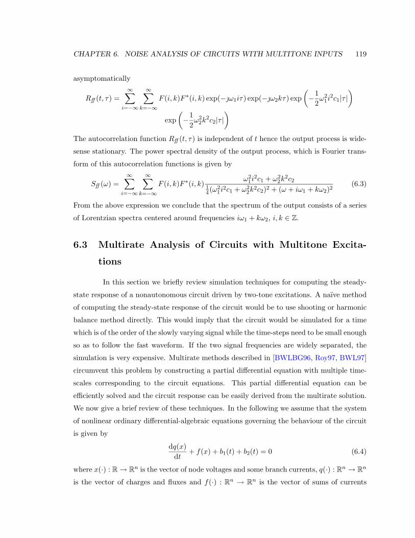
CHAPTER 6. NOISE ANALYSIS OF CIRCUITS WITH MULTITONE INPUTS 119
asymptomatically
Rff (t, τ) =∞∑
i=−∞
∞∑k=−∞
F (i, k)F ∗(i, k) exp(−ω1iτ) exp(−ω2kτ) exp(−1
2ω2
1i2c1|τ |
)exp
(−1
2ω2
2k2c2|τ |
)The autocorrelation function Rff (t, τ) is independent of t hence the output process is wide-
sense stationary. The power spectral density of the output process, which is Fourier trans-
form of this autocorrelation functions is given by
Sff (ω) =∞∑
i=−∞
∞∑k=−∞
F (i, k)F ∗(i, k)ω2
1i2c1 + ω2
2k2c2
14(ω2
1i2c1 + ω2
2k2c2)2 + (ω + iω1 + kω2)2
(6.3)
From the above expression we conclude that the spectrum of the output consists of a series
of Lorentzian spectra centered around frequencies iω1 + kω2, i, k ∈ Z.
6.3 Multirate Analysis of Circuits with Multitone Excita-
tions
In this section we briefly review simulation techniques for computing the steady-
state response of a nonautonomous circuit driven by two-tone excitations. A naıve method
of computing the steady-state response of the circuit would be to use shooting or harmonic
balance method directly. This would imply that the circuit would be simulated for a time
which is of the order of the slowly varying signal while the time-steps need to be small enough
so as to follow the fast waveform. If the two signal frequencies are widely separated, the
simulation is very expensive. Multirate methods described in [BWLBG96, Roy97, BWL97]
circumvent this problem by constructing a partial differential equation with multiple time-
scales corresponding to the circuit equations. This partial differential equation can be
efficiently solved and the circuit response can be easily derived from the multirate solution.
We now give a brief review of these techniques. In the following we assume that the system
of nonlinear ordinary differential-algebraic equations governing the behaviour of the circuit
is given by
dq(x)dt
+ f(x) + b1(t) + b2(t) = 0 (6.4)
where x(·) : R→ Rn is the vector of node voltages and some branch currents, q(·) : Rn → R
n
is the vector of charges and fluxes and f(·) : Rn → Rn is the vector of sums of currents

CHAPTER 6. NOISE ANALYSIS OF CIRCUITS WITH MULTITONE INPUTS 120
entering each node and branch voltages, both depending on x(t). Furthermore, b1(·), b2(·) :
R→ Rn are the vector of input sources which are periodic with period T1 and T2 respectively
and, as before
ω1 =2πT1
and ω2 =2πT2
We also assume that ω1 and ω2 are incommensurable, i.e., for all i, k ∈ Z we have
iω1 + kω2 = 0 iff i = 0 and k = 0
This implies that functions of the kind
exp((iω1 + kω2)t)
are linearly independent for all i, k ∈ Z.
Since the circuit is nonautonomous, we can assume that the steady-state response
xs(t) is quasi-periodic and can be expressed as
xs(t) =∞∑
i=−∞
∞∑k=−∞
Xs(i, k) exp((iω1 + kω2)t) (6.5)
Let xs(t1, t2) be the bivariate form of xs(t), where, as before, xs and xs satisfy the following
relation
xs(t, t) = xs(t)
and let
b(t1, t2) = b1(t1) + b2(t2)
As a suitable generalization of (6.4) for two dimensional functions we consider the
following partial differential equation.
∂q(x(t1, t2))∂t1
+∂q(x(t1, t2))
∂t2+ f(x(t1, t2)) + b(t1, t2) = 0 (6.6)
Considering this partial DAE only for solutions of the form (6.5) implicitly imposes the
following boundary conditions
x(0, t2) = x(T1, t2) (6.7)
x(t1, 0) = x(t1, T2) (6.8)
The following theorem, due to [BWLBG96, Roy97], relates the solution xs(t1, t2) of (6.6)
to the solution xs(t) of (6.4):

CHAPTER 6. NOISE ANALYSIS OF CIRCUITS WITH MULTITONE INPUTS 121
Theorem 6.1 ([BWLBG96, Roy97]) The DAE (6.4) has a quasi-periodic solution xs(t)
iff the partial DAE (6.6) has a solution xs(t1, t2) of the form (6.5). The two solutions are
related by
xs(t) = xs(t, t)
for all t ∈ R.
(6.6) can be solved by the following three different classes of techniques
1. Equations in both time scales t1 and t2 can be solved in time domain [Roy97] either
by using multivariate finite difference time domain method or hierarchal shooting.
• In the multivariate finite difference time domain method the t1, t2 plane is suit-
ably gridded on the rectangle [0, T1]× [0, T2] resulting in a grid of size m1 ×m2.
The partial differential operators of (6.6) are discretized using a linear multistep
method and (6.6) is collocated on the grid. This leads to a set of nonlinear
algebraic equations in the unknowns which is solved using a Newton-Raphson
method. The collocation leads to a system of m = m1 × m2 equations. The
m1 +m2 extra unknowns which result from the discretization of the differential
operators at t1 = 0 and t2 = 0 are eliminated using the bi-periodic boundary
conditions (6.7) and (6.7). The resulting nonlinear system of equations is solved
using Newton-Raphson technique. The Jacobian of size (nm1m2)× (nm1m2) for
the linearized system is of the following p-cyclic form [Roy97]
D1 −Lm1
−L1 D2
−L2 D3
. . . . . .
−Ln1−1 Dn1
Each block (of size (nm2)×(nm2)) is itself an m2×m2 block matrix with p-cyclic
or diagonal structure. Each block is in turn a sparse matrix of size n, consisting
of circuit conductance and capacitance matrices. Hence the overall Jacobian is
extremely sparse and diagonally dominant hence easily amenable to solving using
iterative linear algebra techniques.
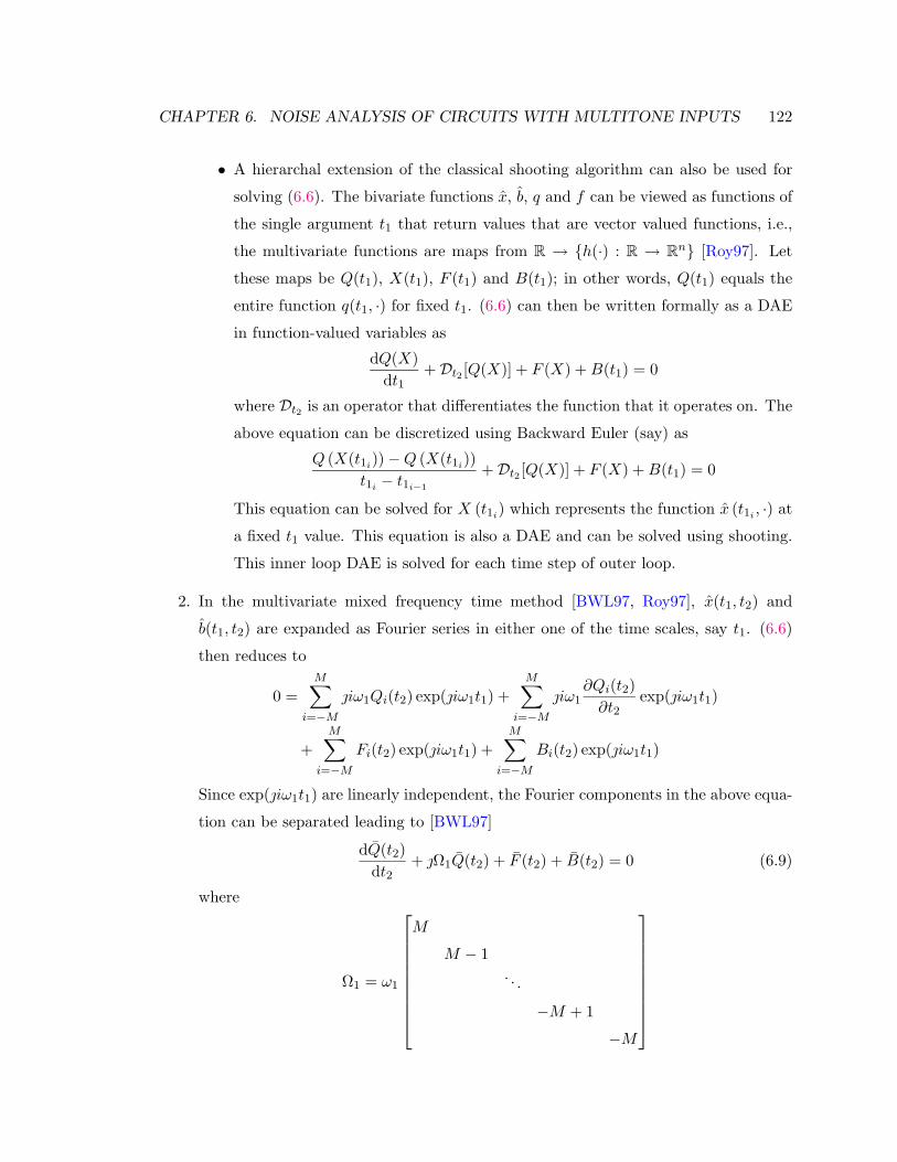
CHAPTER 6. NOISE ANALYSIS OF CIRCUITS WITH MULTITONE INPUTS 122
• A hierarchal extension of the classical shooting algorithm can also be used for
solving (6.6). The bivariate functions x, b, q and f can be viewed as functions of
the single argument t1 that return values that are vector valued functions, i.e.,
the multivariate functions are maps from R → h(·) : R → Rn [Roy97]. Let
these maps be Q(t1), X(t1), F (t1) and B(t1); in other words, Q(t1) equals the
entire function q(t1, ·) for fixed t1. (6.6) can then be written formally as a DAE
in function-valued variables as
dQ(X)dt1
+Dt2 [Q(X)] + F (X) +B(t1) = 0
where Dt2 is an operator that differentiates the function that it operates on. The
above equation can be discretized using Backward Euler (say) as
Q (X(t1i))−Q (X(t1i))t1i − t1i−1
+Dt2 [Q(X)] + F (X) +B(t1) = 0
This equation can be solved for X (t1i) which represents the function x (t1i , ·) at
a fixed t1 value. This equation is also a DAE and can be solved using shooting.
This inner loop DAE is solved for each time step of outer loop.
2. In the multivariate mixed frequency time method [BWL97, Roy97], x(t1, t2) and
b(t1, t2) are expanded as Fourier series in either one of the time scales, say t1. (6.6)
then reduces to
0 =M∑
i=−Miω1Qi(t2) exp(iω1t1) +
M∑i=−M
iω1∂Qi(t2)∂t2
exp(iω1t1)
+M∑
i=−MFi(t2) exp(iω1t1) +
M∑i=−M
Bi(t2) exp(iω1t1)
Since exp(iω1t1) are linearly independent, the Fourier components in the above equa-
tion can be separated leading to [BWL97]
dQ(t2)dt2
+ Ω1Q(t2) + F (t2) + B(t2) = 0 (6.9)
where
Ω1 = ω1
M
M − 1. . .
−M + 1
−M

CHAPTER 6. NOISE ANALYSIS OF CIRCUITS WITH MULTITONE INPUTS 123
Q =
QM
QM−1
...
Q−M+1
Q−M
F =
FM
FM−1
...
F−M+1
F−M
and
B =
BM
BM−1
...
B−M+1
B−M
(6.9) being a vector DAE can be solved in time domain using either finite difference
method or shooting.
3. Yet another method for solving (6.6) is to assume that xs(t1, t2) is of the form
xs(t1, t2) =∞∑
i=−∞
∞∑k=−∞
Xs(i, k) exp((iω1t1 + kω2t2))
and solve for Xs(i, k) directly [BWLBG96]. To this end we assume that the bivariate
versions of the waveforms x(t), f(x(t)) and q(x(t)) are of the form
y(t1, t2) =I∑
i=−I
K∑k=−K
Y (i, k) exp((iω1t1 + kω2t2))
where I and K are chosen such that the truncation error is sufficiently small. Now
y(t1, t2) is restricted to the line [BWLBG96]
y(t) = y
(t1 = t, t2 =
ω1
ω2
12K + 1
t
)(6.10)

CHAPTER 6. NOISE ANALYSIS OF CIRCUITS WITH MULTITONE INPUTS 124
Along this line
t2 =ω1
ω2
12K + 1
t1
the function y is periodic with period T0 = (2K+1)T1 and angular frequency ω0 = 2πT0
.
Therefore
y(t) =I∑
i=−I
K∑k=−K
Y (i, k) exp(
(iω1t+ kω1
12K + 1
t
))
=I∑
i=−I
K∑k=−K
Y (i, k) exp((i(2K + 1) + k)ω0t
)=
L∑l=−L
Y (l) exp(lω0t)
(6.11)
The two sets of coefficients Y (i, k) and Y (l) are related one-to-one by the following
mapping
Y (i, k) = Y (i(2K + 1) + k) (6.12)
and
Y = Y
(i =
(l +K)− (l +K) mod (2K + 1)2K + 1
, k = l − i(2K + 1))
(6.13)
The artificial spectrum is dense and equally spaced hence optimal for FFT operation.
This method transforms the quasi-periodic waveform x(t1, t2) into the periodic wave-
form x(t) using (6.13). The nonlinear relations f(x(t1, t2)) and q(x(t1, t2)) and its
partial derivatives are now evaluated along the line(t1 = t, t2 =
ω1
ω2
12K + 1
t
)and transformed into the frequency domain by a 1-dimensional FFT of size (2I+1)×(2K + 1).
Figure 6.1 shows the output of the four diode mixer described in Section 5.7.1 with a
2.5 GHz 10 dBm RF tone and a 2.2 GHz LO signal. The output corresponds to the
following representation
x(t) =I∑
i=−I
K∑k=−K
X(i, k) exp[(iω1 + kω2)t]

CHAPTER 6. NOISE ANALYSIS OF CIRCUITS WITH MULTITONE INPUTS 125
0 1000 2000 3000 4000 5000 6000 7000 8000 9000 10000−0.08
−0.06
−0.04
−0.02
0
0.02
0.04
0.06
0.08
Sample Points
Out
put V
olta
ge
Figure 6.1: x(t) representation of the output of a four diode mixer
It consists of signals of various frequency mixes of the two large tones and requires
10000 sample points to represent it. Figure 6.2 shows the same output in the repre-
sentation x(t) described by (6.10). This requires only 225 points for representation.
Even though the resemblance to x(t) is minimal, this waveform captures all the har-
monic information of x(t). Moreover, x(t) is periodic allowing conventional harmonic
balance analysis to be used. If the frequency separation between the two tones is very
large or very small then the savings by using the quasi-periodic formulation are even
more dramatic.
6.4 Noise Analysis of Circuits Driven by Multitone Excita-
tions
We now describe our noise analysis technique for nonautonomous circuits driven
by two large signals with phase noise. We again assume that the noiseless steady-state

CHAPTER 6. NOISE ANALYSIS OF CIRCUITS WITH MULTITONE INPUTS 126
0 50 100 150 200−0.08
−0.06
−0.04
−0.02
0
0.02
0.04
0.06
0.08
Sample Points
Out
put V
olta
ge
Figure 6.2: x(t) representation of the output of a four diode mixer
solution of the circuit xs is of the form
xs(t) =∞∑
i=−∞
∞∑k=−∞
Xs(i, k) exp(iω1t) exp(kω2t)
The corresponding bivariate form [BWLBG96, BWL97, Roy97] of xs(t) is given by
xs(t1, t2) =∞∑
i=−∞
∞∑k=−∞
Xs(i, k) exp(iω1t1) exp(kω2t2)
Appealing to the above bivariate form and using arguments similar to those in Section 5.3
we assume that when the input signals are corrupted by Brownian motion phase errors, i.e.,
are of the form b1(t+ α1(t)) and b2(t+ α2(t)), the solution of (6.2) is of the form
xtwo tone = xn(t) + y(t) (6.14)
where
xn(t) =∞∑
i=−∞
∞∑k=−∞
Xs(i, k) exp(iω1(t+ α1(t))
)exp(kω2(t+ α2(t))
)

CHAPTER 6. NOISE ANALYSIS OF CIRCUITS WITH MULTITONE INPUTS 127
From Section 6.2 the spectrum of xn(t) consists of a series of Lorentzians centered
around frequencies iω1 + kω2, i, k ∈ Z. y(t) consists of a wide band noise term (among
possibly other terms). However for the multitone case, the spectrum due to xn(t) is non-
negligible at the output frequency of interest (fIF ). The large blocker signal mixes with the
local oscillator signal to result in a large signal close to (but not exactly at) the intermedi-
ate frequency. The Lorentzian centered at |fLO − fBLOCKER| causes a nonnegligible noise
power at the intermediate frequency.
We need to substitute the form of the solution (6.14) in (6.2). Similar to Sec-
tion 5.3, we first assume that the circuit itself is noiseless, i.e., D(x) = 0. We first make the
following useful observations:
Definition 6.1 Let
s(t) =
s1(t)
s2(t)
=
1
1
dt+
√c1 0
0√c2
dB1(t)
dB2(t)
(6.15)
Lemma 6.2 s(t) as defined in (6.15) is a 2-dimensional Ito process.
Hence we can use the following generalization of Lemma 5.2 to evaluate dxtwo tone .
Lemma 6.3 (The general Ito formula [Øks98]) Let
dX = udt+ vdB
be an n-dimensional Ito process. Let
g(t, x) =
g1(t, x)
...
gp(t, x)
be a twice continuously differentiable map R+ × Rn → R
p. Then the process
Y (t) = g(t,X(t))
is also p-dimensional Ito process whose kth component is given by
dYk =∂gk∂t
(t,X(t))dt+∑i
∂gk∂xi
(t,X(t))dXi +12
∑i
∑j
∂2gk∂x1∂x2
(t,X(t))dXidXj
where
dBidBj = δi,jdt
CHAPTER 6. NOISE ANALYSIS OF CIRCUITS WITH MULTITONE INPUTS 128
Using the result of Lemma 6.3, we can evaluate dxn(t) as:
dxn(t) =∞∑
i=−∞
∞∑k=−∞
Xs(i, k)iω1 exp[iω1(t+ α1(t))
]exp[kω2(t+ α2(t))
](dt+
√c1dB1(t))
+∞∑
i=−∞
∞∑k=−∞
Xs(i, k)kω2 exp[iω1(t+ α1(t))
]exp[kω2(t+ α2(t))
](dt+
√c2dB2(t))
− 12
∞∑i=−∞
∞∑k=−∞
Xs(i, k)i2ω21 exp
(iω1(t+ α1(t))
)exp(kω2(t+ α2(t))
)c1dt
− 12
∞∑i=−∞
∞∑k=−∞
Xs(i, k)k2ω22 exp
(iω1(t+ α1(t))
)exp(kω2(t+ α2(t))
)c2dt
=∞∑
i=−∞
∞∑k=−∞
Xs(i, k)(iω1 + kω2 −
12c1i
2ω21 −
12c2k
2ω22
)exp(iω1(t+ α1(t))
)exp(kω2(t+ α2(t))
)dt
+∞∑
i=−∞
∞∑k=−∞
Xs(i, k)iω1√c1 exp
(iω1(t+ α1(t))
)exp(kω2(t+ α2(t))
)dB1(t)
+∞∑
i=−∞
∞∑k=−∞
Xs(i, k)jω2√c2 exp
(iω1(t+ α1(t))
)exp(kω2(t+ α2(t))
)dB2(t)
The noiseless circuit equation driven by input signals with phase noise is given by
dx(t) = f(x)dt+ b1(t+ α1(t))dt+ b2(t+ α2(t))dt (6.16)
We assume that the solution of this equation is of the form xn(t) + y1(t). Since y1(t) is
assumed to be small compared to xn(t), f(x) in (6.16) can be linearized around xn(t). Then
(6.16) can be rewritten as
dxn(t) + dy1(t) = f(xn(t))dt+∂f(x)∂x
∣∣∣∣xn(t)
y1(t)dt+ b1(t+ α1(t))dt+ b2(t+ α2(t))dt
Also since xs(t1, t2) is bi-periodic, f(xs(t1, t2)) can be written in bivariate form as
f(xs(t1, t2)) =∞∑
i=−∞
∞∑k=−∞
F (i, k) exp((iω1t1 + kω2t2)) (6.17)
Similarly
∂f(x)∂x
∣∣∣∣xs(t1,t2)
=∞∑
i=−∞
∞∑k=−∞
J(i, k) exp((iω1t1 + kω2t2)) (6.18)
We know that xs(t) is a solution of (6.1) iff xs(t1, t2) of the form
xs(t1, t2) =∞∑
i=−∞
∞∑k=−∞
Xs(i, k) exp((iω1t1 + kω2t2)) (6.19)

CHAPTER 6. NOISE ANALYSIS OF CIRCUITS WITH MULTITONE INPUTS 129
is the solution of
∂x(t1, t2)∂t1
+∂x(t1, t2)∂t2
= f(x(t1, t2)) + b1(t1) + b2(t2) (6.20)
and xs(t) = xs(t, t). Substituting (6.19) and (6.17) in (6.20) we have∞∑
i=−∞
∞∑k=−∞
Xs(i, k)iω1 exp((iω1t1 + kω2t2))
+∞∑
i=−∞
∞∑k=−∞
Xs(i, k)kω2 exp((iω1t1 + kω2t2))
=∞∑
i=−∞
∞∑k=−∞
F (i, k) exp((iω1t1 + kω2t2)) + b1(t1) + b2(t2)
This expression is valid for all t1 and t2, in particular t1 +α1(t1) and t2 +α2(t2). Therefore,∞∑
i=−∞
∞∑k=−∞
Xs(i, k)iω1 exp[[iω1(t1 + α1(t1)) + kω2(t2 + α2(t2))
]]+
∞∑i=−∞
∞∑k=−∞
Xs(i, k)kω2 exp[[iω1(t1 + α1(t1)) + kω2(t2 + α2(t2))
]]=
∞∑i=−∞
∞∑k=−∞
F (i, k) exp[[iω1(t1 + α1(t1)) + kω2(t2 + α2(t2))
]]+ b1(t1 + α1(t1)) + b2(t2 + α2(t2))
(6.21)
The corresponding expression in one time scale is obtained by substituting t1 = t2 = t in
the above expression. (6.16) can be written as∞∑
i=−∞
∞∑k=−∞
Xs(i, k)[iω1 + kω2 −
c1i2ω2
1 + c2k2ω2
2
2
]exp[iω1(t+ α1(t)) + kω2(t+ α2(t))
]dt
+∞∑
i=−∞
∞∑k=−∞
Xs(i, k)iω1√c1 exp
(iω1(t+ α1(t))
)exp(kω2(t+ α2(t))
)dB1(t)
+∞∑
i=−∞
∞∑k=−∞
Xs(i, k)jω2√c2 exp
(iω1(t+ α1(t))
)exp(kω2(t+ α2(t))
)dB2(t) + dy1(t)
=∞∑
i=−∞
∞∑k=−∞
F (i, k) exp[[iω1(t+ α1(t)) + kω2(t+ α2(t))
]]dt
+∞∑
i=−∞
∞∑k=−∞
J(i, k) exp[[iω1(t+ α1(t)) + kω2(t+ α2(t))
]]y1(t)dt+ b1(t+ α1(t))dt
+ b2(t+ α2(t))dt
(6.22)

CHAPTER 6. NOISE ANALYSIS OF CIRCUITS WITH MULTITONE INPUTS 130
Using the equality (6.21), (6.22) becomes
dy1(t) =∞∑
i=−∞
∞∑k=−∞
J(i, k) exp[[iω1(t+ α1(t)) + kω2(t+ α2(t))
]]y1(t)dt
+∞∑
i=−∞
∞∑k=−∞
Xs(i, k)c1i
2ω21 + c2k
2ω22
2exp(iω1(t+ α1(t))
)exp(kω2(t+ α2(t))
)dt
−∞∑
i=−∞
∞∑k=−∞
Xs(i, k)iω1√c1 exp
(iω1(t+ α1(t))
)exp(kω2(t+ α2(t))
)dB1(t)
−∞∑
i=−∞
∞∑k=−∞
Xs(i, k)kω2√c2 exp
(iω1(t+ α1(t))
)exp(kω2(t+ α2(t))
)dB2(t)
(6.23)
The above stochastic differential equation is linear in y1(t). This means that y1(t) can be
viewed as y1(t) = y11(t) + y12(t) where y11(t) satisfies the following stochastic differential
equation
dy11(t) =∞∑
i=−∞
∞∑k=−∞
J(i, k) exp[[iω1(t+ α1(t)) + kω2(t+ α2(t))
]]y11(t)dt
−∞∑
i=−∞
∞∑k=−∞
Xs(i, k)iω1√c1 exp
(iω1(t+ α1(t))
)exp(kω2(t+ α2(t))
)dB1(t)
−∞∑
i=−∞
∞∑k=−∞
Xs(i, k)kω2√c2 exp
(iω1(t+ α1(t))
)exp(kω2(t+ α2(t))
)dB2(t)
(6.24)
and y12(t) satisfies the following stochastic differential equation
dy12(t) =∞∑
i=−∞
∞∑k=−∞
J(i, k) exp[[iω1(t+ α1(t)) + kω2(t+ α2(t))
]]y12(t)dt
+∞∑
i=−∞
∞∑k=−∞
Xs(i, k)c1i
2ω21 + c2k
2ω22
2exp(iω1(t+ α1(t))
)exp(kω2(t+ α2(t))
)dt
(6.25)
The input terms in (6.24) correspond to two independent white noise sources which are
modulated by
−√c1∂xs(t1, t2)
∂t1
∣∣∣∣t1=t+α1(t),t2=t+α2(t)
and
−√c2∂xs(t1, t2)
∂t2
∣∣∣∣t1=t+α1(t),t2=t+α2(t)

CHAPTER 6. NOISE ANALYSIS OF CIRCUITS WITH MULTITONE INPUTS 131
Using similar arguments as in Section 5.3, we can conclude that y11(t) is the stationary
component of z11(t) where z11(t) is governed by the following linear stochastic differential
equation
dz11(t) =∞∑
i=−∞
∞∑k=−∞
J(i, k) exp[(iω1 + kω2)t
]z11(t)dt
−√c1∂xs(t1, t2)
∂t1
∣∣∣∣t1=t2=t
dB1(t)−√c2∂xs(t1, t2)
∂t2
∣∣∣∣t1=t2=t
dB2(t)
(6.26)
Using similar arguments as in Section 5.3 it also follows that y12(t) in (6.25) is a
deterministic bi-periodic signal except that it is corrupted by phase deviation terms α1(t)
and α2(t) of the two input signals b1(t+α1(t)) and b2(t+α2(t)). Since the original system
is nonautonomous, it follows that for small c1 and c2, i.e., small input signal phase noise,
y12(t) is small compared to xn(t). The spectrum of y12(t) is similar to the spectrum of xn(t)
except that it is of much smaller amplitude. Hence the effect of adding y12(t) to the output
is to change the amplitude of the spectrum of the original signal xn(t) without altering its
frequency content.
It is easy to argue that when circuit noise sources are also included, i.e., D(x) 6= 0,
the output process can be expressed as xn(t) + y0(t) and
y0(t) = y01(t) + y12(t)
Here y12(t) is the same as defined in (6.25) and y01(t) is the stationary component of z01(t)
where z01(t) is governed by
dz01(t) =∞∑
i=−∞
∞∑k=−∞
J(i, k) exp[(iω1 + kω2)t
]z01(t)dt−
√c1∂xs(t1, t2)
∂t1
∣∣∣∣t1=t2=t
dB1(t)
−√c2∂xs(t1, t2)
∂t2
∣∣∣∣t1=t2=t
dB2(t) +D(xs(t))dBp(t)
(6.27)
This equation is very similar to the one obtained using conventional two tone noise analysis.
The only difference is the addition to two white noise sources, appropriately modulated and
the fact that we only need to consider the stationary component of output noise. This result
can be generalized to the case when l large input signals are present. It can be shown that
l additional white noise terms of the form
−√ci∂xs(t1, . . . , tl)
∂ti
∣∣∣∣t1=...=tl=t
1 ≤ i ≤ l

CHAPTER 6. NOISE ANALYSIS OF CIRCUITS WITH MULTITONE INPUTS 132
are added to the circuit noise equations. In the next section we describe how to compute
the statistics of the output noise z01(t) for the bi-periodic case.
6.5 Numerical Techniques
We begin by describing the conventional small signal and noise analysis of a nonau-
tonomous circuit driven by two large incommensurable tones. We will derive expressions
for the output noise statistics in terms of the input noise statistics and the linear transfer
function. We use the property that a bi-periodic signal, when approximated by a truncated
two dimensional Fourier series and its time axis suitably warped, is in fact a periodic signal
for an appropriate frequency. The bi-periodic noise analysis problem reduces to a periodic
noise analysis problem and we can use techniques described in Section 5.6. In particular,
the frequency domain technique can be easily extended for the bi-periodic case. Therefore,
we only discuss the frequency domain technique here.
Consider (6.1) with a steady-state solution of the form (6.5). We consider the case
when the large input signals b1(t) and b2(t) are noiseless and the system of equations is
perturbed by additive noise as D(x(t))ξ(t) and is given by
dxdt
= f(x(t)) + b1(t) + b2(t) +D(x(t))ξ(t) (6.28)
and the solution is assumed to be of the form
x(t) = xs(t) + y(t)
and y(t) is assumed to be small for small perturbation D(x(t))ξ(t). Substituting this in
(6.28) we have
dxsdt
+dydt
= f(xs(t) + y(t)) + b1(t) + b2(t) +D(xs(t) + y(t))ξ(t)
Linearizing the nonlinear function f(xs(t)+y(t)) around the large unperturbed steady-state
solution xs(t) and ignoring y(t) in the argument of D(x) in the above equations we have
dxsdt
+dydt
= f(xs(t)) + J(xs(t))y(t) + b1(t) + b2(t) +D(xs(t))ξ(t) (6.29)
where
J(xs(t)) =∂f(x)∂x
∣∣∣∣xs(t)

CHAPTER 6. NOISE ANALYSIS OF CIRCUITS WITH MULTITONE INPUTS 133
Since xs(t) is the solution of (6.1), (6.29) reduces to
dydt
= J(xs(t))y(t) +D(xs(t))ξ(t) (6.30)
The above differential equation is linear in y(t). Since xs(t) is bi-periodic, the coefficient
matrix J(xs(t)) is bi-periodic. Hence this equation represents as linear bi-periodic time
varying transfer function. We now describe propagation of noise through a linear bi-periodic
time varying system. The derivation is along the lines of that described in Section 5.6 for
periodic case. The extension to general quasi-periodic case is immediate.
6.5.1 Propagation of Noise Through a Liner Quasi-Periodic Time Varying
System
(6.30) is a linear differential equation (in y(t)) with bi-periodic coefficient matrix.
This equation represents a linear bi-periodic transfer function h(t2, t1) which implies that
this transfer function is periodic with respect to displacements of T1 and T2 in both its
arguments, i.e., h(t2 + T1, t1 + T1) = h(t2, t1) and h(t2 + T2, t1 + T2) = h(t2, t1). The
bi-periodicity of h implies that it can be expanded as
h(t2, t1) =∞∑
i=−∞
∞∑k=−∞
hi,k(t2 − t1) exp((iω1 + kω2)t) (6.31)
hi,k(·) are called bi-harmonic impulse responses of the linear bi-periodic time varying system.
Their Fourier transforms Hi,k(ω) are called bi-harmonic transfer functions of the system,
i.e.,
Hi,k(ω) =∫ ∞−∞
hi,k(t) exp(−ωt)dt (6.32)
Since circuit noise are in general nonstationary stochastic processes, their covariance matrix
is defined as Ruu(t1, t2) = E
[u(t1)uT (t2)
]where u is the input noise source. The output
noise x is related to the input noise as
Rxx(t1, t2) = E
[x(t1)xT (t2)
]= E
[∫ ∞−∞
∫ ∞−∞
h(t1, s1)u(s1)uT (s2)hT (s2, t1)ds1ds2
]=∫ ∞−∞
∫ ∞−∞
h(t1, s1)Ruu(s1, s2)hT (t2, s2)ds1ds2
The two dimensional Fourier transform of Rxx(t1, t2) is defined as
Sxx(ω3, ω4) =∫ ∞−∞
∫ ∞−∞
Rxx(t1, t2) exp(−(ω3t1 + ω4t2)
)dt1dt2

CHAPTER 6. NOISE ANALYSIS OF CIRCUITS WITH MULTITONE INPUTS 134
Substituting (6.31) and (6.32) in the above expression of Sxx(ω3, ω4) we have
Sxx(ω3, ω4) =
∞∫∫∫∫−∞
h(t1, s1)Ruu(t1, t2)h(t2, s2) exp(−(ω3t1 + ω4t2)
)ds1ds2dt1dt2
=1
16π4
∫∫∫ ∞∫∫−∞
∫∫∫ ∞∑i,k,l,m=−∞
Hi,k(ω7) exp((ω7(t1 − s1) + (iω1 + kω2)t1
))Suu(ω5, ω6) exp
((ω5s1 + ω6s2)
)HTl,m(ω8)
exp((ω8(t2 − s2) + (lω1 +mω2)t2
))exp
(− (ω3t1 + ω4t2)
)ds1ds2dt1dt2dω5dω6
dω7dω8
=1
16π4
∫∫∫ ∞∫∫−∞
∫∫∫ ∞∑i,k,l,m=−∞
Hi,k(ω7)Suu(ω5, ω6)HTl,m(ω8) exp
((ω5 − ω7)s1
)exp((ω6 − ω8)s2
)exp((ω7 + iω1 + kω2 − ω3)t1
)exp((ω8 + lω1 +mω2 − ω4)t2
)ds1ds2dt1dt2dω5
dω6dω7dω8
=
∞∫∫∫∫−∞
∞∑i,k,l,m=−∞
Hi,k(ω7)Suu(ω5, ω6)HTl,m(ω8)δ(ω5 − ω7)δ(ω6 − ω8)
δ(ω7 + iω1 + kω2 − ω3)δ(ω8 + lω1 +mω2 − ω4)
dω5dω6dω7dω8
=∫ ∞−∞
∫ ∞−∞
∞∑i,k,l,m=−∞
Hi,k(ω5)Suu(ω5, ω6)HTl,m(ω6)δ(ω5 + iω1 + kω2 − ω3)
δ(ω6 + lω1 +mω2 − ω4)dω5dω6
=∞∑
i,k,l,m=−∞Hi,k(ω3 − iω1 − kω2)Suu(ω3 − iω1 − kω2, ω4 − lω1 −mω2)
HTl,m(ω4 − lω1 −mω2)
(6.33)
Here we have used the fact that
12π
∫ ∞−∞
exp(ωt)dt = δ(ω)

CHAPTER 6. NOISE ANALYSIS OF CIRCUITS WITH MULTITONE INPUTS 135
Since xs(t) is bi-periodic, the coefficient matrix D(xs(t)) in (6.29) is also bi-periodic. Hence
the statistics of circuit noise sources are also bi-periodic. This implies that Rxx and Ruu do
not change if T1 or T2 are added to both their arguments, i.e.,
Rpp(t1 + T1, t2 + T1) = Rpp(t1 + T2, t2 + T2) = Rpp(t1, t2)
Hence both can be expanded in Fourier series as
Rpp(t1, t2) =∞∑
i=−∞
∞∑k=−∞
Rppi,k(t2 − t1) exp((iω1 + kω2)t
)Rxxi,k and Ruui,k are known as bi-harmonic covariances of the input and output noise
respectively. Their Fourier transform is referred to as bi-harmonic power spectral density
and is given by
Sppi,k(ω) =∫ ∞−∞
Rppi,k exp(−ωt)dt
With the assumption that input and output noise autocorrelations are bi-periodic with
respect to T1 and T2, the two-dimensional power spectral densities of input and output
noise are given by
Spp(ω3, ω4) =∫ ∞−∞
∫ ∞−∞
Rpp exp(−(ω3t1 + ω4t2)
)dt1dt2
=∫ ∞−∞
∫ ∞−∞
∞∑i=−∞
∞∑k=−∞
Rppi,k(t2 − t1) exp((iω1 + kω2 − ω4)t2 − ω3t1)
)dt1dt2
=1
2π
∞∫∫∫−∞
∞∑i=−∞
∞∑k=−∞
Sppi,k(ω) exp((iω1 + kω2 − ω4)t2 − ω3t1)
)exp(ω(t2 − t1)
)dωdt1dt2
= 2π∫ ∞−∞
∞∑i=−∞
∞∑k=−∞
Sppi,k(ω)δ(−ω3 − ω)δ(iω1 + kω2 − ω4 + ω)dω
= 2π∞∑
i=−∞
∞∑k=−∞
Sppi,k(−ω3)δ(ω4 + ω3 − iω1 − kω2)
Using the above form in (6.33) we have
2π∞∑
i=−∞
∞∑k=−∞
Sxxi,k(−ω3)δ(ω3 + ω4 − iω1 − kω2)
=2π∞∑
l,m,n,p,q,r=−∞Hl,m(ω3 − lω1 −mω2)Suun,p(−ω3 + lω1 +mω2)
δ(ω3 + ω4 − (l + n+ q)ω1 − (p+m+ r)ω2
)HTq,r(ω4 − qω1 − rω2)

CHAPTER 6. NOISE ANALYSIS OF CIRCUITS WITH MULTITONE INPUTS 136
Therefore
Sxxi,k(−ω) =∞∑
l,m,n,p=−∞Hl,m(ω − lω1 −mω2)Suun,p(−ω + lω1 +mω2)
HTi−(l+n),k−(m+p)
(−ω − (l + n)ω1 − (m+ p)ω2
) (6.34)
In an actual RF circuit, the signal bandwidth is limited and hence a finite number harmonics
of signals are present. Hence the infinite summations in all the above expressions are
truncated. We assume that harmonics corresponding to ω1 are truncated to ±I and the
harmonics corresponding to ω2 are truncated to ±K. Hence a bi-periodic waveform z(t) in
this system is given by
z(t) =I∑
i=−I
K∑k=−K
Z(i, k) exp((iω1 + kω2)t
)The bivariate form of this signal is given by
z(t1, t2) =I∑
i=−I
K∑k=−K
Z(i, k) exp((iω1t1 + kω2t2)
)Consider the waveform z(t) which obtained from z(t1, t2) by constraining it on the line
(6.10). z(t) is periodic with a period T0 = (2K + 1)T1 and can be written as
z(t) =L∑
i=−LZ(l) exp(lω0t)
where
ω0 =2π
(2K + 1)T1
and
L =(2I + 1)(2K + 1)− 1
2= 2IK + I +K
The one-to-one mapping between the harmonics present in the circuit and the
artificial spectrum [Kun89] is given by (6.12) and (6.13) and is depicted in Figure 6.3. Note
that z(t) is derived from z(t) by suitably distorting the time axis. If z(t) is not required in
the intermediate calculation, then the entire analysis can be carried out using the artificial

CHAPTER 6. NOISE ANALYSIS OF CIRCUITS WITH MULTITONE INPUTS 137
i
k
Figure 6.3: Illustration of the AFM method for a box truncation scheme with two incom-mensurable frequencies
spectrum. The advantage is that we can reuse the analysis developed previously for the
periodic case. For instance, if the summations in (6.34) are truncated then
Sxxi,k(−ω) =I∑
l,n=−I
K∑m,p=−K
Hl,m(ω − lω1 −mω2)Suun,p(−ω + lω1 +mω2)
HTi−(l+n),k−(m+p)
(−ω − (l + n)ω1 − (m+ p)ω2
) (6.35)
for −I ≤ i ≤ I and −K ≤ k ≤ K. (6.35) can be written in terms of S and H as
Sxxi =L∑
l=−L
L∑n=−L
Hl(ω − lω0)Suun(−ω + lω0)Hi−l−n(−ω + (l + n)ω0
)This expression is exactly the same as the one derived for the periodic case in Section 5.6.2.1.
6.5.2 Derivation of the Form of Transfer Function
Consider (5.17) which is repeated here for convenience
C(t)y +G(t)y +Ab(t) = 0
CHAPTER 6. NOISE ANALYSIS OF CIRCUITS WITH MULTITONE INPUTS 138
where G(t) and C(t) are assumed to be bi-periodic with periods T1 and T2. We further
assume that system of equations is nonautonomous. Since (5.17) is linear in y(t), the
corresponding linear bi-periodic time varying transfer function h(t2, t1) can be written as
h(t2, t1) =∞∑
i=−∞
∞∑k=−∞
hi(t2 − t1) exp[(iω1 + kω2)t2]
=1
2π
∫ ∞−∞
∞∑i=−∞
∞∑k=−∞
Hi,k(ω) exp[ω(t2 − t1)] exp[(iω1 + kω2)t2]dω
For the purpose of this analysis we assume that b(t) is deterministic and its Fourier transform
is given by
B(ω) =∫ ∞−∞
b(t) exp(−ωt)dt
Since h(t2, t1) is the linear transfer function corresponding to (5.17), we have
y(t2) =∫ ∞−∞
h(t2, t1)b(t1)dt1
=1
4π2
∞∫∫∫−∞
∞∑i=−∞
∞∑k=−∞
Hi,k(ω3) exp[ω3(t2 − t1)] exp[(iω1 + kω2)t2]B(ω4) exp(ω4t1)
dω3dω4dt1
=1
2π
∫ ∞−∞
∫ ∞−∞
∞∑i=−∞
∞∑k=−∞
Hi,k(ω3) exp[(ω3 + iω1 + kω2)t2]B(ω4)δ(ω4 − ω3)dω3dω3
=1
2π
∞∑i=−∞
∞∑k=−∞
∫ ∞−∞
Hi,k(ω)B(ω) exp[(ω + iω1 + kω2)t2]dω
This implies that the Fourier transform of x(t) is given by
Y (ω) =∞∑
i=−∞
∞∑k=−∞
Hi,k(ω − iω1 − kω2)B(ω − iω1 − 2ω2)
(5.17) is rewritten as
0 =1
2π
∫ ∞−∞
∞∑i=−∞
∞∑k=−∞
Ci,k exp[(iω1 + kω2)t]ωY (ω) exp(ωt)dω
+1
2π
∫ ∞−∞
∞∑i=−∞
∞∑k=−∞
Gi,k exp[(iω1 + kω2)t]Y (ω) exp(ωt)dω
+1
2π
∫ ∞−∞
AB(ω) exp(ωt)dω

CHAPTER 6. NOISE ANALYSIS OF CIRCUITS WITH MULTITONE INPUTS 139
Fourier transform of the above expression is given by∞∑
i=−∞
∞∑k=−∞
Ci,k(ω − iω1 − kω2)Y (ω − iω1 − kω2) +∞∑
i=−∞
∞∑k=−∞
Gi,kY (ω − iω1 − kω2)
+AB(ω) = 0
Substituting the value of Y (ω) in the above expression we have∞∑
i,k,l,m=−∞Ci,k[ω − iω1 − kω2]Hl,m[ω − (i+ l)ω1 − (k +m)ω2]
B[ω − (i+ l)ω1 − (k +m)ω2]
+∞∑
i,k,l,m=−∞Gi,kHl,m[ω − (i+ l)ω1 − (k +m)ω2]B[ω − (i+ l)ω1 − (k +m)ω2]
+AB(ω) = 0
Since the above expression is valid for every B(ω), it must be necessary that for i + l = 0
and k +m = 0∞∑
i=−∞
∞∑k=−∞
(ω − iω1 − kω2)Ci,kH−i,−k(ω) +∞∑
i=−∞
∞∑k=−∞
Gi,kH−i,−k(ω) +A = 0 (6.36)
and for i+ l = n 6= 0 or k +m = p 6= 0 we have∞∑
i=−∞
∞∑k=−∞
(ω − iω1 − kω2)Ci,kHn−i,p−k(ω − nω1 − pω2)
+∞∑
i=−∞
∞∑k=−∞
Ci,kHn−i,p−k(ω − nω1 − pω2) = 0
(6.37)
Collocating (6.36) the terms at frequencies ω − nω1 − pω2 for all n, p ∈ Z we have∞∑
i=−∞
∞∑k=−∞
[ω − (i+ n)ω1 − (k + p)ω2]Ci,kH−i,−k(ω − nω1 − pω2)
+∞∑
i=−∞
∞∑k=−∞
Ci,kH−i,−k(ω − nω1 − pω2) +A = 0
(6.38)
To evaluate (6.37) and (6.38) we again appeal to the AFM technique introduced
in Section 6.5.1. If the infinite summations in these equations are truncated to ±I and
±K respectively and an artificial frequency map constructed as in Section 6.5.1, (6.37) and
(6.38) can be written as
L∑i=−L
(ω − iω0)CiHn−i(ω − nω0) +L∑
i=−L
CiHn−i(ω − nω0) = 0
CHAPTER 6. NOISE ANALYSIS OF CIRCUITS WITH MULTITONE INPUTS 140
and for all n ∈ ZL∑
i=−L
[ω − (i+ n)ω0]CiH−i(ω − nω0) +L∑
i=−L
CiH−i(ω − nω0) +A = 0
These equations are very similar to (5.26) and (5.27) and hence the technique outlined in
Section 5.6.2 for the periodic case can be used to perform noise analysis.
6.6 Examples
We carried out a two tone analysis of the two mixers described in Section 5.7. In
addition to the 2.2 GHz LO signal, a large blocker signal at 2.5 GHz was applied at the RF
port. For the active mixer, the RF signal power was set to −10 dBm while for the passive
mixer, it was set to 10 dBm. The noise figure for the active mixer increased by 2.1 dB in
presence of the blocker signal. The corresponding increase in the noise of passive mixer was
computed to be 4.1 dB. The LO and blocker signals were assumed to be noiseless for this
analysis. This increase in NF in entirely due the fact that the large blocker signals drive the
linear signal path of these mixers into gain compression which decreases the signal power
and decreases the overall SNR.
The analysis was carried out using 225 frequency mixes and took approximately
six minutes for the passive mixer and 9.5 minutes for the active mixer on a 600 MHz
Digital Alpha workstation. In our implementation, since Spice3 was used for transient
simulation, the circuit waveforms and Jacobian matrices were converted to the bi-periodic
representation. This conversion required an additional (30%) overhead. Since in an actual
multitone implementation, this overhead will not be present, it is not reported in the above
run times.
The blocker signal gets downconverted to a frequency which is at 300 MHz, i.e,
100 MHz away from the IF signal. If either the blocker or LO signal have phase noise, then
according to (6.3) the output spectrum consists of a Lorentzian centered at 300 MHz. The
noise contributed to the output by this can be significant specially if the blocker frequency
is very close to the RF signal frequency. In addition, the wide band noise due to the phase
noise of the two large tones also increases the overall output noise of the mixer. Figures 6.4
and 6.5 plot the increase in noise figure due to phase noise in the two large tones.
We observe that the presence of a large blocker signal increases the sensitivity of
the circuit to input signal phase noise. Comparing these figures to Figures 5.3 and 5.5 we

CHAPTER 6. NOISE ANALYSIS OF CIRCUITS WITH MULTITONE INPUTS 141
1e−221e−21
1e−201e−19
1e−181e−17
1e−16
1e−22
1e−21
1e−20
1e−19
1e−18
1e−17
1e−1615
20
25
30
35
40
45
c1 (sec2Hz)c
2 (sec2Hz)
NF
(dB
)
Figure 6.4: Increase in noise figure due to phase noise in the two input signal for the fourdiode mixer
1e−201e−19
1e−181e−17
1e−161e−15
1e−14
1e−20
1e−19
1e−18
1e−17
1e−16
1e−15
1e−145
10
15
20
25
30
35
c1 (sec2Hz)c
2 (sec2Hz)
NF
(dB
)
Figure 6.5: Increase in noise figure due to phase noise in the two input signal for the Gilbertcell mixer

CHAPTER 6. NOISE ANALYSIS OF CIRCUITS WITH MULTITONE INPUTS 142
find that the crossover point where the mixer noise figure starts increasing with ci is reduced
by about an order of magnitude. For the four diode mixer, we observed in Section 5.7 that
due to perfectly symmetry, the output node was insensitive to LO signal phase noise. The
presence of a large blocker destroys this symmetry and makes the output node susceptible
to phase noise from both RF and LO signals. Therefore, blocker performance constraint
poses much stricter constraints on the noise performance of input signal than just the one
tone noise performance constraint.
143
Chapter 7
Conclusions and Future Directions
In this chapter we summarize our contributions and point out to some future
directions where this research can proceed.
7.1 Conclusions
In this work we have investigated noise analysis and modelling problem for RF
circuits. We first concentrated on noise analysis of autonomous circuits and then turned
our attention to noise analysis of nonautonomous circuits which are driven by oscillators
which have phase noise. We summarize our contributions below:
• We showed that linear perturbation analysis is not valid for oscillatory circuits. This
analysis predicts that the deviation away from the unperturbed steady-state solution
keeps increasing unbounded even for the smallest of perturbations. It was shown that
noise analysis techniques for oscillators which are based on linear perturbation analysis
predict nonphysical effects such as infinite total integrated noise power density.
• We developed a new perturbation analysis technique which is valid for oscillators. We
showed that the perturbed oscillator response can be viewed as a sum of two signals:
periodic steady-state unperturbed oscillator response time shifted by an amount α(t)
and a small and bounded deviation away from the limit cycle. We derived a nonlinear
differential equation for α(t), found the component of perturbation term that causes
deviation only along the limit cycle of the form xs(t+α(t)) and showed that when we
add in the rest of the perturbation term, it causes only small and bounded deviations

CHAPTER 7. CONCLUSIONS AND FUTURE DIRECTIONS 144
away from the limit cycle for all times. In terms of this phase plane interpretation we
precisely defined the notion of phase error, phase deviation and amplitude deviation.
• For white noise perturbations, the nonlinear differential equation for phase error α(t)
becomes a stochastic differential equation and we used techniques from stochastic cal-
culus to obtain a second order characterization of phase error and oscillator response.
We showed that oscillator response, as a stochastic process, is wide-sense stationary.
We gave arguments for the physical interpretation of this result.
• We then addressed the noise analysis problem of nonautonomous circuits driven by
a single large periodic signal which has phase noise. We argued that since a nonau-
tonomous circuit, along with the driving oscillator, can be viewed as a composite
oscillator, the output noise process will be stationary and not cyclostationary, as
would be predicted by classical noise analysis for such circuits. We also derived this
result mathematically. We showed that the effect of input signal phase noise is to add
another white noise source to the circuit noise sources which is modulated by the time
derivative of the noiseless steady-state response of the circuit.
• We extended this analysis for nonautonomous circuits driven by multi-tone excita-
tions. We first reviewed some techniques in time domain, frequency domain and
mixed time frequency domain techniques for simulating circuits driven by two large
incommensurable frequency signals. We then discussed noise analysis techniques for
these circuits.
7.2 Noise Models for Circuits Driven by Multitone Excita-
tions
A byproduct of oscillator phase noise analysis presented in Chapter 4 was a com-
pact and accurate noise model for oscillator output. We showed that a single scalar constant
c is sufficient for modelling a noisy oscillator output. We later used this model in Chap-
ters 5 and 6 for noise analysis of nonautonomous circuits. We also gave a noise model for
nonautonomous circuit driven by an input signal with phase noise in terms of a stochastic
differential equation. A similar model can be developed of the output of a nonautonomous
circuit driven by two or more large periodic signals with phase noise. One possible choice

CHAPTER 7. CONCLUSIONS AND FUTURE DIRECTIONS 145
of the model would be the stochastic differential equation similar to the one we developed
in Chapter 5.
7.3 Extensions to Non-White Noise Sources
Other than thermal and shot noise sources, there are other circuit noise sources
that cannot be modelled as a white noise source. The most important of them is flicker noise
which has a power spectral density inversely proportional to frequency. This represents a
problem since total integrated noise power in any finite bandwidth around DC is infinite.
This noise source cannot be modelled as a well defined stochastic process and hence is not
amenable to be handled using stochastic differential equation theory. The approximation of
replacing the flicker noise source with a series of white noise sources can be used. However,
the asymptotic arguments that were presented throughout this exposition need not be valid
and need to be revisited. Consider the oscillator phase noise equation (4.1) (which is
repeated here)
dα(t)dt
= vT (t+ α(t))ξ(t)
where v is small, i.e., of the order ε. Let t′ = tε and let us rewrite the above equation as
dα(t)dt
= vT(t+ α
(t′
ε
))ξ
(t′
ε
)The averaging principle [FW84] states that at time t′ = O(1), α would be governed by [Zei98]
dαdt
= gξ
(t′
ε
)For white noise sources ξ(t), it immediately follows that α is a Brownian motion process.
Now consider a low pass filtered white noise source. The low pass filter can be absorbed
in the circuit equations and we can conclude that asymptotically α is still a Brownian
motion. If the correlation time is sufficiently small, then at time O(1/ε), the noise source
would appear almost white and the asymptotic argument will be valid. However, if the
correlation time is comparable to O(1/ε), then the noise source does not appear white and
the asymptotic argument is not valid. This is certainly the case for flicker noise where
the correlation time is comparable, if not larger than the measurement time. Even though
flicker noise is a low frequency phenomenon, in nonlinear circuits, it can mix with periodic
signals and get shifted to frequencies of interest. Extending this analysis to handle the
flicker noise case in a consistent manner is a very important problem.

CHAPTER 7. CONCLUSIONS AND FUTURE DIRECTIONS 146
7.4 Behavioural Level Noise Simulation
Once noise model for nonautonomous circuits driven by multitone excitation is
in place, behavioural level noise analysis techniques for RF circuits need to be developed
which utilize these models for nonautonomous and autonomous circuits. These techniques
would also be based on the solution of appropriate stochastic differential equations. The
behavioural level noise analysis would enable a system designer to quickly evaluate different
choices of architectures for RF front-ends for noise performance and investigate various
design trade-offs. This would possibly also enable the use of techniques in the digital
domain to recover some noise performance, given the particular characterization of noise
from the RF front end.
In conjunction with component level models and system level simulation techniques
for distortion and other nonidealities in the system, this effort will hopefully enable efficient
design of high performance RF systems. We believe that a more thorough understanding
of how noise and other nonidealities affect the overall circuit response will be crucial in
minimizing overdesign which exists in current RF design practices. Specifically for RF mo-
bile systems, this would result in lower power and hence higher battery life. Equivalently,
extra functionality can be incorporated in those parts of an RF system where lower power
dissipation is not an important issue (such as base stations of RF communication systems).

147
Bibliography
[ABR76] J Robert Ashley, Thomas A Barley, and Gustaf J Rast, Jr. Automated spectral
analysis of microwave oscillator noise. In 1976 IEEE MTT-S International
Microwave Symposium, pages 227–229, 1976. 2.3.1
[AKR94] Werner Anzill, Franz X Kartner, and Peter Russer. Simulation of the phase
noise of oscillators in the frequency domain. Archiv fur Elektronik und
Ubertragungstechnik, 48(1):45–50, January 1994. 2.3.1
[AM83] Asad A Abidi and Robert G Meyer. Noise in relaxation oscillators. IEEE
Journal of Solid-State Circuits, SC–18(6):794–802, December 1983. 2.3.2,
4.6.4, 4.6.4
[AM97] Krzysztof Antoszkiewicz and Janusz Markowski. Computer aided noise anal-
ysis of an oscillator. Bulletin of the Polish Academy of Sciences, Technical
Sciences, 45(1):183–195, 1997. 2.3.1
[Arn74] Ludwig Arnold. Stochastische Differentialgleichungen: Theorie und Anwen-
dung. John Wiley & Sons, 1974. 4.1, 4.1.2, 4.1.2
[AT72a] Thomas J Aprille, Jr. and Timothy N Trick. A computer algorithm to deter-
mine the steady-state response of nonlinear oscillators. IEEE Transactions on
Circuit Theory, CT19(4):354–360, July 1972. 4.5.1
[AT72b] Thomas J Aprille, Jr. and Timothy N Trick. Steady-state analysis of nonlinear
circuits with periodic inputs. Proceedings of the IEEE, 60(1):108–114, January
1972. 4.5.1
[Ber84] Jeremy Bernstein. Three degrees above zero : Bell Labs in the information
age. New York : C. Scribner’s, 1984. (document)

BIBLIOGRAPHY 148
[BWL97] Hans-Georg Brachtendorf, Gunther Welsch, and Rainer Laur. A novel time-
frequency method for the simulation of the steady state of circuits driven by
multi-tone signals. In Proceedings of the 1997 IEEE International Symposium
on Circuits and Systems, volume 3, pages 1508–1511, 1997. 6.2, 6.3, 2, 2, 6.4
[BWLBG96] Hans-Georg Brachtendorf, Gunther Welsch, Rainer Laur, and Angelika Bunse-
Gerstner. Numerical steady state analysis of electronic circuits driven by
multi-tone signals. Electrical Engineering, 79:103–112, 1996. 6.2, 6.3, 6.3,
6.1, 3, 3, 6.4
[Che91] Jonathan Y C Cheah. Analysis of phase noise in oscillators. RF Design,
14(12):99–100, 1991. 2.3.1
[CHG95] Chang-Li Chen, Xing-Nan Hong, and Bao-Xin Gao. A new and efficient
approach to the accurate simulation of phase noise in microwave MESFET
oscillators. In 1995 SBMO/IEEE MTT-S International Microwave and Op-
toelectronics Conference Proceedings, pages 230–234, 1995. 2.3.1
[Dek87] Astrid P Dekker. Approximate noise analysis of a feedback oscillator using a
nonlinear differential amplifier. Archiv fur Elektronik und Ubertragungstechnik,
41(3):129–132, 1987. 2.3.4
[DLSV96] Alper Demir, Edward Liu, and Alberto Sangiovanni-Vincentelli. Time-domain
non Monte-Carlo noise simulation for nonlinear dynamic circuits with arbi-
trary excitations. IEEE Transactions for Computer-Aided Design, 15:493–505,
May 1996. 2.2.2, 2.3.3, 5.7.2
[Dob93] Janusz A Dobrowolski. CAD oriented method for noise analysis of microwave
circuits described by the nodal admittance matrix. IEE Proceedings H Mi-
crowaves, Antennas and Propagation, 140(4):321–325, August 1993. 2.2.2
[DSG97] Bart De Smedth and George Gielen. Accurate simulation of phase noise in os-
cillators. In Proceedings of the 23rd European Solid-State Circuits Conference,
pages 208–211, 1997. 2.3.1
[DSV96] Alper Demir and Alberto Sangiovanni-Vincentelli. Simulation and modeling of

BIBLIOGRAPHY 149
phase noise in open-loop oscillators. In Proceedings of the IEEE 1996 Custom
Integrated Circuits Conference, pages 453–456, 1996. 2.3.3
[DTS98a] Aleksander Dec, Laszlo Toth, and Ken Suyama. Noise analysis of a class of
oscillators. IEEE Transactions on Circuits and Systems II: Analog and Digital
Signal Processing, 45(6):757–60, June 1998. 2.3.1, 4.6.1, 4.4(b), 4.6.1
[DTS98b] Aleksander Dec, Laszlo Toth, and Ken Suyama. Noise analysis of an oscillator
with an M th-order filter and comparator-type nonlinearity. In Proceedings of
the 1998 IEEE International Symposium on Circuits and Systems, volume 1,
pages 225–228, 1998. 2.3.1
[FAOR95] Tilman Felgentreff, Werner Anzill, Gerhard Olbrich, and Peter Russer. Analy-
sis of g-r noise upconversion in oscillators. In 1995 IEEE MTT-S International
Microwave Symposium Digest, pages 947–950, 1995. 2.3.1
[Far94] Miklos Farkas. Periodic Motions. Applied mathematical sciences. Springer–
Verlag, New York, 1994. 1, 1, 3.2, 3.1, 3.5
[FHM97] Keng L Fong, Christopher D Hull, and Robert G Meyer. A class AB mono-
lithic mixer for 900-MHz applications. IEEE Journal of Solid-State Circuits,
32(8):1166–1172, August 1997. 3
[FM99] Keng L Fong and Robert G Meyer. Monolithic RF active mixer design. IEEE
Transactions on Circuits and Systems–II: Analog and Digital Signal Process-
ing, 46(3):231–239, March 1999. 1.1
[FV88] Gerard J Foschini and Giovanni Vannucci. Characterizing filtered light
waves corrupted by phase noise. IEEE Transactions on Information Theory,
34(6):1437–1448, November 1988. 2.3.4
[FW84] Mark I Freidlin and Alexander D Wentzell. Random Perturbations of Dynam-
ical Systems. Springer–Verlag, 1984. 7.3
[Gar83] Crispin W Gardiner. Handbook of stochastic methods for physics, chemistry,
and the natural sciences, volume 13 of Springer series in synergetics. Springer–
Verlag, Berlin, Heidelberg, New York, Tokyo, second edition, 1983. 4.1, 4.1,
4.1.2, 4.1.2

BIBLIOGRAPHY 150
[Gar90] William A Gardner. Introduction to Random Processes : with Applications
to Signals and systems. McGraw–Hill, New York, second edition, 1990. 4.2,
4.3.2
[Gha96] Ranjit Gharpurey. Modeling and analysis of substrate coupling in integrated
circuits. PhD thesis, University of California at Berkeley, 1996. 1.2.1, 1.2.1
[GM93] Paul R Gray and Robert G Meyer. Analysis and design of Analog Integrated
Circuits. Wiley, New York, third edition, 1993. 4.6.4
[GM95] Paul R Gray and Robert G Meyer. Future directions in silicon ICs for RF
personal communications. In Proceedings of the IEEE 1995 Custom Integrated
Circuits Conference, pages 83–90, 1995. 1.1, 1.1
[Gol89] Jules Goldberg. Nonlinear analysis of high Q oscillator phase noise. In Pro-
ceedings of the 43rd Annual Symposium on Frequency Control 1989, pages
63–74, 1989. 2.3.4
[Gri90] Roger Grimshaw. Nonlinear ordinary differential equations. Applied mathe-
matics and engineering science texts. Blackwell Scientific Publications, Oxford,
Boston, 1990. 3.2, 3.4.3, 3.4.3, 5.1, 6.1
[GS92] Geoffrey R Grimmett and David R Stirzaker. Probability and random pro-
cesses. Oxford University Press, New York, second edition, 1992. 4.1, 1,
4.1.2, 4.1.2, 4.2
[Haf66] Erich Hafner. The effect of noise in oscillators. Proceedings of the IEEE,
54(2):179–198, February 1966. 2.3.1
[Hag81] Peter Hagedorn. Nichtlineare Schwingungen. Oxford University Press, 1981.
3.4.1
[HK77] Daniel N Held and Anthony R Kerr. Analysis of noise in room-temperature
millimeter-wave mixers. In 1977 International Microwave Symposium Digest,
pages 483–486, 1977. 2.2.1
[HKK98] Robert L Howald, Stan Kesler, and Moshe Kam. BER performance analysis
of OFDM-QAM in phase noise. In Proceedings. 1998 IEEE International
Symposium on Information Theory, page 256, 1998. 1.2.2

BIBLIOGRAPHY 151
[HKW91] Stefan Heinen, Jurgen Kunisch, and Ingo Wolff. A unified framework for
computer-aided noise analysis of linear and nonlinear microwave circuits.
IEEE Transactions on Microwave Theory and Techniques, 39(12):2170–2175,
December 1991. 2.2.1
[HL98] Ali Hajimiri and Thomas H Lee. A general theory of phase noise in electrical
oscillators. IEEE Journal of Solid-State Circuits, 33(2):179–94, February 1998.
2.3.1
[HM93] Christopher D Hull and Robert G Meyer. A systematic approach to the
analysis of noise in mixers. IEEE Transactions on Circuits and Systems I:
Fundamental Theory and Applications, 40(12):909–919, December 1993. 2.2.1
[Hud92] Premysl Hudec. Procedures for exact noise analysis of microwave circuits.
Microwave Journal, 35(9):165–170, September 1992. 2.2.1
[Hul92] Christopher D Hull. Analysis and Optimization of Monolithic RF Downcon-
version Receivers. PhD thesis, University of California, Berkeley, 1992. 2.2.1
[Kar90] Franz X Kartner. Analysis of white and f−α noise in oscillators. International
Journal of Circuit Theory and Applications, 18(5):485–519, October 1990.
2.3.4
[Kin98] Peter Kinget. A fully integrated 2.7 V 0.35 µm CMOS VCO for 5 GHz wireless
applications. In Digest of Technical Papers IEEE International Solid-State
Circuits Conference, pages 226–227, 1998. 4.6.2, 4.6.2
[Kun89] Kenneth S Kundert. Steady state methods for simulating analog circuits. PhD
thesis, University of California at Berkeley, 1989. 6.5.1
[Kur68] Kaneyuki Kurokawa. Noise in synchronized oscillators. IEEE Transactions
on Microwave Theory and Techniques, MTT-16(4):234–40, 1968. 2.3.1
[KWSV90] Kenneth S Kundert, Jacob K White, and Alberto L Sangiovanni-Vincentelli.
Steady-state methods for simulating analog and microwave circuits. Kluwer
Academic Publishers, Boston ; Dordrecht, 1990. 1, 4.5.1
[Lax67] Melvin Lax. Classical noise. v. noise in self-sustained oscillators. Physical
Review, CAS–160:290–307, 1967. 2.3.4
BIBLIOGRAPHY 152
[Lee66] David B Leeson. A simple model of feedback oscillator noise spectrum. Pro-
ceedings of the IEEE, 54(2):329–330, February 1966. 2.3.1
[McN97] John A McNeill. Jitter in ring oscillators. IEEE Journal of Solid-State Cir-
cuits, 32(6):177–193, June 1997. 2.3.2, 4.3.4, 4.6.3, 4.6.3, 4.6.3, 4.6.3, 4.6.3
[MK82] Kohji Motoishi and Tosiro Koga. Simulation of a noise source with 1/f spec-
trum by means of an RC circuit. Electronics and Communications in Japan,
65-A(3):19–27, March 1982. 1.2.1
[Nez98] Mohammad K Nezami. Phase noise analysis. 1. evaluate the impact of phase
noise on receiver performance. Microwaves & RF, 37(5):165–166, May 1998.
1.2.2
[NM79] Ali Hasan Nayfeh and Dean T Mook. Nonlinear Oscillations. John Wiley &
Sons, 1979. 3.4.1
[Ohi93] Takashi Ohira. Higher-order analysis on phase noise generation in varactor-
tuned oscillators-baseband noise upconversion in GaAs MESFET oscillators.
IEICE Transactions on Electronics, E76-C(12):1851–1854, December 1993.
2.3.1
[Øks98] Bernt K Øksendal. Stochastic differential equations: an introduction with
applications. Springer–Verlag, 1998. 2.2, 2.2, 4.1, 4.1.1, 4.1.2, 4.1.2, 5.2, 5.2,
6.3, A
[OT97] Makiko Okumura and Hiroshi Tanimoto. A time-domain method for numerical
noise analysis of oscillators. In Proceedings of the Asia South Pacific Design
Automation Conference, pages 477–82, January 1997. 2.3.1
[OTS91] Makiko Okumura, Hiroshi Tanimoto, and Tsutomu Sugawara. Noise analysis
method for nonlinear circuits with two frequency excitations using the com-
puter. Electronics and Communications in Japan Part 3, 74(4):41–50, 1991.
2.2.1
[Pap91] Athanasios Papoulis. Probability, Random Variables and Stochastic Processes.
McGraw Hill, third edition, 1991. 5.3
BIBLIOGRAPHY 153
[Pat96] Andrew Patterson. Computer aided analysis of noise effects in GSM. Elec-
tronic Engineering, 68(838):53–54, 1996. 1.2
[Poo97] Rick Poore. Accurate simulation of mixer noise and oscillator phase noise in
large RFICs. In 1997 Asia-Pacific Microwave Conference Proceedings APMC
’97, pages 357–360, 1997. 2.3.1
[Raz96] Behzad Razavi. A study of phase noise in CMOS oscillators. IEEE Journal
of Solid-State Circuits, 31(3):331–43, March 1996. 2.3.1, 2.3.1
[RC95] Ulrich L Rohde and Chao-Ren Cheng. Analysis and optimization of oscillators
for low phase noise and low power consumption. RF Design, 18(3):70–79,
March 1995. 2.3.1
[RCMC94] Vittorio Rizzoli, Alessandra Costanzo, Franco Mastri, and Claudio Cecchetti.
Harmonic-balance optimization of microwave oscillators for electrical perfor-
mance, steady-state stability, and near-carrier phase noise. In Proceedings of
IEEE/MTT-S International Microwave Symposium, pages 1401–4, May 1994.
2.3.1
[RFL98] Jaijeet S Roychowdhury, Peter Feldmann, and David E Long. Cyclostationary
noise analysis of large RF circuits with multi-tone excitations. IEEE Journal
of Solid-State Circuits, 33(3):324–36, March 1998. 2.2.1, 2.2.1, 4.5.2, 4.3,
4.5.2, 5.2, 5.6, 5.6.2, 5.6.2.1, 5.6.2.1, 5.6.2.2, 5.7
[Ris96] Hannes Risken. The Fokker-Planck equation : methods of solution and appli-
cations, volume 18 of Springer series in synergetics. Springer–Verlag, Berlin ;
New York, second edition, 1996. 4.1
[RM92] Peter Russer and Stefan Muller. Noise analysis of microwave circuits with
general topology. In 1992 IEEE MTT-S International Microwave Symposium
Digest, volume 3, pages 1481–1484, 1992. 2.2.1
[RMC89] Vittorio Rizzoli, Franco Mastri, and Claudio Cecchetti. Computer-aided noise
analysis of MESFET and HEMT mixers. IEEE Transactions on Microwave
Theory and Techniques, 37(9):1401–1410, September 1989. 2.2.1

BIBLIOGRAPHY 154
[RMC98] Vittorio Rizzoli, Franco Mastri, and Claudio Cecchetti. Signal and noise anal-
ysis of large microwave front-ends by the inexact-newton harmonic-balance
technique. In 1998 IEEE MTT-S International Microwave Symposium Di-
gest, volume 3, pages 1599–1602, 1998. 2.2.1
[RMM92a] Vittorio Rizzoli, Diego Masotti, and Franco Mastri. Advanced piecewise-
harmonic-balance noise analysis of nonlinear microwave circuits with appli-
cation to schottky-barrier diodes. In 1992 IEEE MTT-S International Mi-
crowave Symposium Digest, pages 247–250, 1992. 2.2.1
[RMM92b] Vittorio Rizzoli, Diego Masotti, and Franco Mastri. General-purpose noise
analysis of forced nonlinear microwave circuits. In Conference Proceedings
MM 92, pages 293–298, 1992. 2.2.1
[RMM94a] Vittorio Rizzoli, Diego Masotti, and Franco Mastri. Full nonlinear noise anal-
ysis of microwave mixers. In 1994 IEEE MTT-S International Microwave
Symposium Digest, volume 2, pages 961–964, 1994. 2.2.1, 2.2.1
[RMM94b] Vittorio Rizzoli, Franco Mastri, and Diego Masotti. General noise analysis of
nonlinear microwave circuits by the piecewise harmonic-balance techniques.
IEEE Transactions on Microwave Theory and Techniques, 42:807–819, May
1994. 2.2.1, 2.2.1
[RMM95] Vittorio Rizzoli, Diego Masotti, and Franco Mastri. Computer-aided noise
analysis of integrated microwave front-ends. In 1995 IEEE MTT-S Interna-
tional Microwave Symposium Digest, volume 3, pages 1561–1564, 1995. 2.2.1
[RMMN92] Vittorio Rizzoli, Diego Masotti, Franco Mastri, and Andrea Neri. Noise anal-
ysis of a nonlinear microwave circuit driven by a noise sinusoidal source. Mi-
crowave and Optical Technology Letters, 5(10):534–537, September 1992. 2.2.1
[RMMN93] Vittorio Rizzoli, Diego Masotti, Franco Mastri, and Andrea Neri. Full nonlin-
ear analysis of near-carrier noise in discriminator-stabilized microwave oscil-
lators. Microwave and Optical Technology Letters, 6(16):907–911, 1993. 2.3.1
[Rob82] William P Robins. Phase noise in signal sources : theory and applications,

BIBLIOGRAPHY 155
volume 9 of IEE telecommunications series. Peter Peregrinus on behalf of the
Institution of Electrical Engineers, London, 1982. 1.2.2, 2.3.1
[ROC+97] Jacques C Rudell, Jia-Jiunn Ou, Thomas B Cho, George Chien, Francesco
Brianit, Jeffrey A Weldon, and Paul R Gray. A 1.9-GHz wide-band IF double
conversion CMOS receiver for cordless telephone applications. IEEE Journal
of Solid-State Circuits, 32(12):2071–2088, December 1997. 1.1
[RON+98] Jacques C Rudell, Jia-Jiunn Ou, R Sekhar Narayanaswami, George Chien,
Jeffrey A Weldon, Li Lin, King-Chun Tsai, Luns Tee, Kelvin Khoo, Danelle
Au, Troy Robinson, Danilo Gerna, Masanori Otsuka, and Paul R Gray. Recent
developments in high integration multi-standard CMOS transceivers for per-
sonal communication systems. In Proceedings 1998 International Symposium
on Low Power Electronics and Design, pages 149–154, 1998. 1.1
[Roy97] Jaijeet S Roychowdhury. Efficient methods for simulating highly nonlinear
multi-rate circuits. In Proceedings of the 34th Design Automation Conference,
pages 269–274, 1997. 6.2, 6.3, 6.3, 6.1, 1, 1, 1, 2, 6.4
[RPP88] Ulrich L Rohde, Anthony M Pavio, and Robert A Pucel. Accurate noise sim-
ulation of microwave amplifiers using CAD. Microwave Journal, 31(12):130–
141, December 1988. 2.2.1
[Sau77] Gerard Sauvage. Phase noise in oscillators: a mathematical analysis of Lee-
son’s model. IEEE Transactions on Instrumentation and Measurement, IM-
26(4):408–410, December 1977. 2.3.1
[SD98] Oliver Schein and Georg Denk. Numerical solution of stochastic differential-
algebraic equations with applications to transient noise simulation of mi-
croelectronic circuits. Journal of Computational and Applied Mathematics,
100(1):77–92, 1998. 2.2.2
[Sjo72] Anders Sjolund. Analysis of large-signal noise in Read oscillators. Solid-State
Electronics, 15(9):971–978, September 1972. 2.3.1
[SS85] Heinz J Siweris and Burkhard Schiek. Analysis of noise upconversion in mi-

BIBLIOGRAPHY 156
crowave FET oscillators. IEEE Transactions on Microwave Theory and Tech-
niques, MTT-33(3):233–242, March 1985. 2.3.1
[Swe72] Allen A Sweet. A general analysis of noise in Gunn oscillators. Proceedings of
the IEEE, 60(8):999–1000, August 1972. 2.3.1
[TKW96] Ricardo Telichevesky, Kenneth S Kundert, and Jacob K White. Efficient AC
and noise analysis for two-tone RF circuits. In Proceedings of the 33rd Design
Automation Conference, pages 292–297, 1996. 2.2.1, 5.2, 5.6, 5.6.1
[Tom98] Luciano Tomba. Analysis of the effect of phase noise in OFDM systems.
European Transactions on Telecommunications, 9(3):279–287, 1998. 1.2.2
[vdP22] Balthasar van der Pol. On oscillation hysteresis in a simple triode generator.
Philosophical Magazine, 43:177–193, 1922. 3.4
[VLPG96] Jacques Verdier, Olivier Llopis, Robert Plana, and Jacques Graffeuil. Analysis
of noise upconversion in microwave field-effect transistor oscillators. IEEE
Transactions on Microwave Theory and Techniques, 44(8):1478–1483, August
1996. 2.3.1
[VV83] Vincent C Vannicola and Pramod K Varshney. Spectral dispersion of mod-
ulated signals due to oscillator phase instability: White and random walk
phase model. IEEE Transactions on Communications, COM-31(7):886–895,
July 1983. 1.2.2, 2.3.4
[Wei93] Guo Wei. Flicker noise process analysis. In Proceedings of the 1993 IEEE
International Frequency Control Symposium, pages 321–325, 1993. 1.2.1
[WKG94] Todd C Weigandt, Beomsup Kim, and Paul R Gray. Analysis of timing jitter
in CMOS ring oscillators. In Proceedings of IEEE International Symposium
on Circuits and Systems, pages 27–30, 1994. 2.3.2, 4.6.3, 4.6.3, 4.6.3, 4.6.3
[YL97] Jiang Yilin and Xiao Lizhi. Analysis on phase noise for phase-lock radar
frequency synthesizer. In 1997 IEEE International Conference on Intelligent
Processing Systems, volume 1, pages 28–31, 1997. 2.3.1
[Zei98] Ofer Zeitouni. personal communication, 1998. 7.3

157
Appendix A
Definitions and Solution
Techniques of SDEs
Here we summarize the mathematical machinery we needed in Chapter 5. This
material is from [Øks98].
A.1 Mathematical Preliminaries
Definition A.1 If Ω is a given set, then a σ-algebra F on Ω is a family F of the subsets
of Ω with the following properties
1. ∅ ∈ F
2. F ∈ F ⇒ FC ∈ F , where FC = Ω \ F is the complement of F in Ω
3. A1, A2, . . . ∈ F ⇒ A =⋃∞i=1Ai ∈ F
The pair (Ω,F) is called a measurable space. A probability measure P on a
measurable space (Ω,F) is a function P : F → [0, 1] such that
1. P [∅] = 0, P [Ω] = 1
2. if A1, A2, . . . ∈ F and Ai∞i=1 is disjoint then
P
[ ∞⋃i=1
Ai
]=∞∑i=1
P [Ai]

APPENDIX A. DEFINITIONS AND SOLUTION TECHNIQUES OF SDES 158
The triple (Ω,F ,P) is called the probability space.
The subsets F of Ω which belong to F are called F-measurable sets. In a probability context
these sets are called events and we use the interpretation
P [F ] = “the probability that the event F occurs”
In particular, if P [F ] = 1 we say that F occurs with probability 1, or almost surely (a.s.).
Given any family U of subsets of Ω there is a smallest σ-algebra HU containing Unamely
HU =⋂H : H σ-algebra of Ω, U ∈ H
HU is called the σ-algebra generated by U .
For instance, if U is the collection of all open subsets of a topological space Ω (e.g.
Ω = Rn), then B = HU is called the Borel σ-algebra on Ω and the elements B ∈ B are called
Borel sets. B contains all open sets, all closed sets, all countable unions of closed sets, all
countable intersections of such countable unions etc.
If (Ω,F ,P) is a given probability space, then a function Y : Ω → Rn is called
F-measurable if
Y −1(U) = ω ∈ Ω : Y (ω) ∈ U ∈ F
for all open sets U ∈ Rn (or, equivalently, for all Borel sets U ⊂ Rn).
If X : Ω → Rn is any function, then the σ-algebra HX generated by X is the
smallest σ-algebra on Ω containing all the sets
X−1(U) U ⊂ Rn open
It can be shown that
HX = X−1(B) : B ∈ B
where B is the Borel σ-algebra on Rn. Clearly X will then be HX -measurable and HX is
the smallest σ-algebra with this property.

APPENDIX A. DEFINITIONS AND SOLUTION TECHNIQUES OF SDES 159
A.2 Ito Integrals
The following integral is defined as the Ito integral∫ T
Sf(t, ω)dBt(ω)
where Bt(ω) is a 1-dimensional Brownian motion. We need the following definitions to
describe the class of function f(t, ω) for which the Ito integral will be defined.
Definition A.2 Let Bt(ω) be an n-dimensional Brownian motion. Then Ft = F (n)t is
defined to be the σ-algebra generated by the random variables Bs(·), s ≤ t. In other words,
Ft is the smallest σ-algebra containing all sets of the form
ω : Bt1(ω) ∈ F1, . . . , Btk(ω) ∈ Fk
where k = 1, 2 . . . , tj > 0 and Fj ⊂ Rn are Borel sets. (All sets of measure zero are assumed
to be included in Ft.)
Definition A.3 Let Ntt≥0 be a nondecreasing family of σ-algebras of subsets of Ω. A
process g(t, ω) : R+ × Ω→ Rn is called Nt-adapted if for each t ≥ 0 the function
ω → g(t, ω)
is Nt-measurable.
Ito integral can be defined for the following class of functions:
Definition A.4 Let V = V(S, T ) be the class of functions
f(t, ω) : R+ × Ω→ R
such that
1. (t, ω)→ f(t, ω) is B × F-measurable where B denotes the Borel σ-algebra on R+
2. f(t, ω) is Ft adapted
3. E[∫ TS f(t, ω)2dt
]<∞
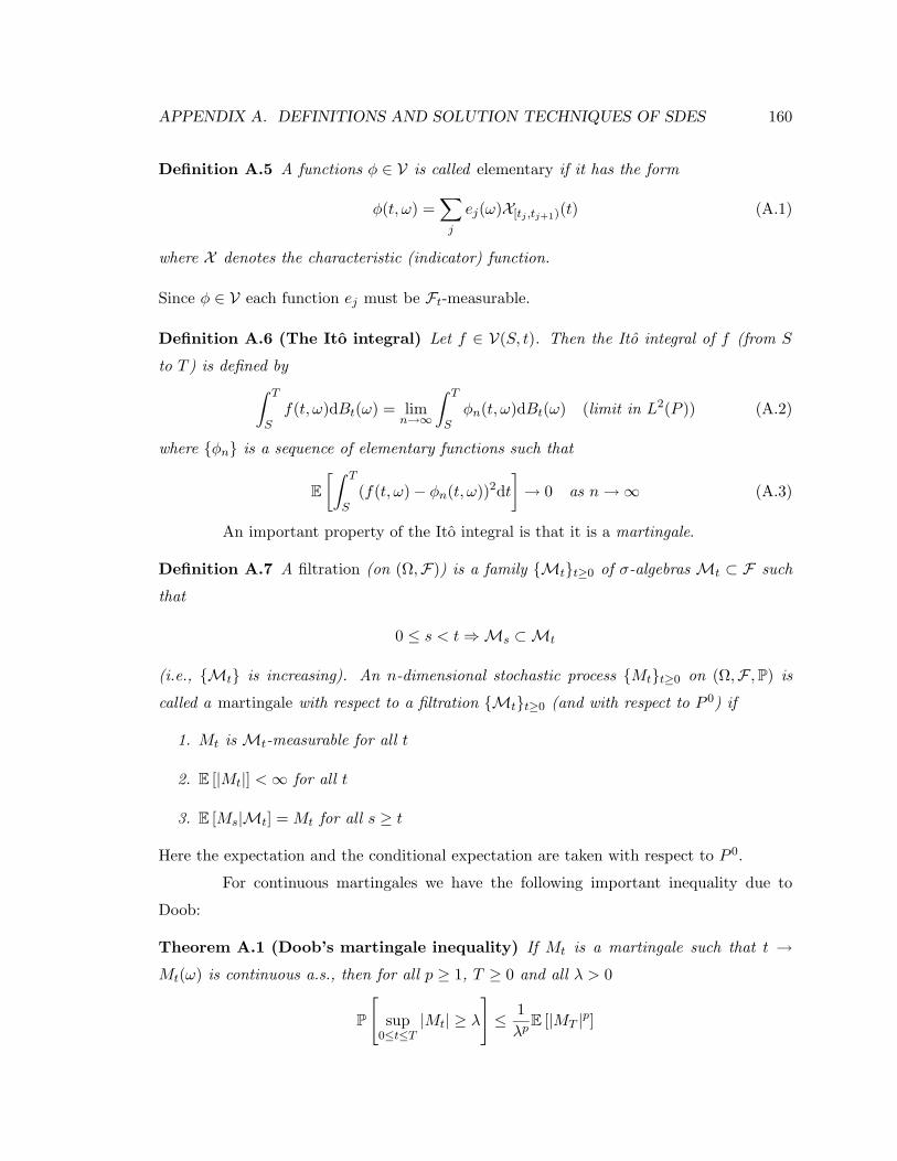
APPENDIX A. DEFINITIONS AND SOLUTION TECHNIQUES OF SDES 160
Definition A.5 A functions φ ∈ V is called elementary if it has the form
φ(t, ω) =∑j
ej(ω)X[tj ,tj+1)(t) (A.1)
where X denotes the characteristic (indicator) function.
Since φ ∈ V each function ej must be Ft-measurable.
Definition A.6 (The Ito integral) Let f ∈ V(S, t). Then the Ito integral of f (from S
to T ) is defined by∫ T
Sf(t, ω)dBt(ω) = lim
n→∞
∫ T
Sφn(t, ω)dBt(ω) (limit in L2(P )) (A.2)
where φn is a sequence of elementary functions such that
E
[∫ T
S(f(t, ω)− φn(t, ω))2dt
]→ 0 as n→∞ (A.3)
An important property of the Ito integral is that it is a martingale.
Definition A.7 A filtration (on (Ω,F)) is a family Mtt≥0 of σ-algebras Mt ⊂ F such
that
0 ≤ s < t⇒Ms ⊂Mt
(i.e., Mt is increasing). An n-dimensional stochastic process Mtt≥0 on (Ω,F ,P) is
called a martingale with respect to a filtration Mtt≥0 (and with respect to P 0) if
1. Mt is Mt-measurable for all t
2. E [|Mt|] <∞ for all t
3. E [Ms|Mt] = Mt for all s ≥ t
Here the expectation and the conditional expectation are taken with respect to P 0.
For continuous martingales we have the following important inequality due to
Doob:
Theorem A.1 (Doob’s martingale inequality) If Mt is a martingale such that t →Mt(ω) is continuous a.s., then for all p ≥ 1, T ≥ 0 and all λ > 0
P
[sup
0≤t≤T|Mt| ≥ λ
]≤ 1λpE [|MT |p]

APPENDIX A. DEFINITIONS AND SOLUTION TECHNIQUES OF SDES 161
This inequality can be used to prove that the Ito integral∫ t
0f(s, ω)dBs
can be chosen to depend continuously on t.
Theorem A.2 Let f ∈ (0, T ). Then there exists a t-continuous version of∫ t
0f(s, ω)dBs(ω) 0 ≤ t ≤ T
i.e., there exists a t-continuous stochastic process Jt on (Ω,F ,P) such that
P
[Jt =
∫ t
0f(s, ω)dBs(ω)
]= 1 ∀t 0 ≤ t ≤ T (A.4)
Corollary A.3 Let f(s, ω) ∈ V(0, T ) for all T . Then
Mt(ω) =∫ t
0f(s, ω)dBs
is a martingale with respect to Ft and
P
[sup
0≤t≤T|Mt| > λ
]≤ 1λ2E
[∫ T
0f(s, ω)2ds
]λ, T > 0 (A.5)
The Ito integral∫fdB can be defined for a larger class of integrands f than V.
First, the measurability condition (2) of Definition A.4 can be relaxed to the following:
2’: There exists an increasing family of σ-algebras Ht t ≥ 0 such that
1. Bt is a martingale with respect to Ht
2. ft is Ht-adapted
Condition 1 implies that Ft ⊂ Ht. The essence of this extension is that we can allow ft
to depend on more than Ft as long as the Bt remains a martingale with respect to the
“history” of fs s ≤ t. If the above conditions hold then E [Bs −Bt|Ht] = 0 for all s > t and
this is sufficient to carry out the construction of Ito integral.
Condition (3) of Definition A.4 can also be weakened to
3′ P
[∫ t
0f(s, ω)2ds <∞ for all t ≥ 0
]= 1
Definition A.8 W denotes a class of stochastic processes satisfying 1 of Definition A.4
and 2’ and 3’ above.

APPENDIX A. DEFINITIONS AND SOLUTION TECHNIQUES OF SDES 162
A.3 Stochastic Differential Equations
Theorem A.4 (Existence and uniqueness theorem) Let T > 0 and b(·, ·) : [0, T ] ×Rn → R
n, σ(·, ·) : [0, T ]× Rn → Rn×m be measurable functions satisfying
|b(t, x)|+ |σ(t, x)| ≤ C(1 + |x|) x ∈ Rn t ∈ [0, T ] (A.6)
for some constant C, where |σ|2 =∑|σij |2 and such that
|b(t, x)− b(t, y)|+ |σ(t, x)− σ(t, y)| ≤ D|x− y| x, y ∈ Rn t ∈ [0, T ] (A.7)
for some constant D. Let Z be a random variation which is independent of the σ-algebra
F∞ generated by Bs(·), s ≥ 0 and such that
E
[|Z|2
]<∞ (A.8)
Then the stochastic differential equation
dXt = b(t,Xt)dt+ σ(t,Xt)dBt 0 ≤ t ≤ T X0 = Z (A.9)
has a unique t-continuous solution Xt(ω) each component of which belongs to V[0, T ].
Remark A.1 Conditions (A.6) and (A.7) are natural in view of the following two simple
examples from deterministic differential equations (i.e., σ = 0):
1. The equation
dXt
dt= X2
t X0 = 1 (A.10)
corresponding to b(x) = x2 (which does not satisfy (A.6)) has the (unique) solution
Xt =1
1− t0 ≤ t < 1
Thus it is impossible to find a global solution (defined for all t) in this case. More
generally, condition (A.6) ensures that the solution Xt(ω) does not explode, i.e., that
|X(ω)| does not tend to ∞ in a finite time.
2. The equation
dXt
dt= 3X2/3
t X(0) = 0 (A.11)

APPENDIX A. DEFINITIONS AND SOLUTION TECHNIQUES OF SDES 163
has more than one solution. In fact for any a > 0 the function
Xt =
0 t ≤ a(t− a)3 t > a
solves (A.11). In this case b(x) = 3x2/3 does not satisfy the Lipschitz condition (A.7)
at x = 0.
Thus condition (A.7) guarantees that equation (A.9) has a unique solution. Here uniqueness
means that if X1(t, ω) and X2(t, ω) are two t-continuous processes in V[0, T ] satisfying (A.9)
then
X1(t, ω) = X2(t, ω) for all t ≥ T a.s. (A.12)

164
Index
σ-algebra, 92, 156
Matlab, 74
Spice, 74
additive noise, 88
amplitude deviation, 32, 36
amplitude noise, 50, 88, 98
asymptotic phase property, 21
Backward Euler method, 102
bit error rate, 6
block Toeplitz matrix, 76
blocker signal, 6, 114
Boltzmann’s constant, 7
Borel σ-algebra, 157
Borel set, 157
Brownian motion, 56, 89, 95, 116, 158
characteristic multiplier, 44
cyclostationary process, 90, 95, 98
downconversion, 3
elementary function, 159
emitter-coupled multivibrator, 85
existence and uniqueness theorem
Picard-Lindelof, 20
flicker noise, 7
Floquet eigenvector, 27
Floquet theory, 23
Fokker-Planck equation, 52, 57, 90
forced oscillator circuit, 89
Fourier transform, 54
Gaussian process, 52, 65, 66
Gaussian random variable, 52, 59
harmonic balance, 75
conversion matrix, 75, 106
harmonic impulse response, 75, 106
harmonic power spectral density, 75, 105
image frequency, 114
image reject mixer, 114
image-reject filter, 3
indicator function, 159
infrared system, 1
inverse Fourier transform, 54
Ito formula, 93
Ito integral, 158, 160
martingale property of, 56, 159
Ito process, 92, 93
jammer signal, 114
Kramers-Moyal expansion, 52
coefficient, 53
Lindstedt-Poincare method, 37

INDEX 165
linear analysis
time invariant, 67
time-varying, 67
Lipschitz condition, 162
Lorentzian spectrum, 64, 67, 81, 100, 118
low noise amplifier, 3
LPTV system of equations, 23, 88, 91, 101
characteristic multipliers, 24
Floquet exponents, 24, 74
fundamental matrix of, 23
principal, 23
state transition matrix, 23
LPTV transfer function, 75
martingale, 92, 159
measurable space, 156
memoryless nonlinearity, 115, 116
mixed differential-algebraic equation, 19,
89
modified nodal analysis, 89
Monte Carlo noise simulation, 83
multitone excitation, 116
noise, 2
coupling, 6
intrinsic, 7
noise analysis, 2
noise source figure of merit, 72
nonautonomous circuit, 88, 89, 116
orbital deviation, 32
orbital stability, 20
asymptotic, 20, 34, 45, 46, 77
oscillator
Colpitt’s, 81
generic, 79
LC tank, 79, 81
relaxation, 79, 85
ring, 79, 83
van der Pol, 37
forced, 40, 42
voltage controlled, 85
oscillator perturbation analysis
linear, 19, 22
nonlinear, 30
oscillator phase noise
analysis
frequency domain, 75
time-domain, 73
spectrum, 64
dBc/Hz, 70
dBm/Hz, 70
perfect time reference, 68
periodic steady-state solution, 101
phase deviation, 31
phase lock loop, 3
phase noise, 50, 88
phase noise/timing jitter sensitivity, 72
Picard-Lindelof Theorem, 23
power amplifier, 3
probability density function, 51
characteristic function, 53, 58
moments, 53
probability measure, 51, 156
probability space, 92, 157
quasi-periodic, 114

INDEX 166
radio frequency system, 1
RF front end, 3
Riemann-Stieljes, 56
shooting method, 73, 74
shot noise, 7
signal to noise ratio, 6
singular matrix, 78
null space of, 78
state transition matrix, 26, 73
stochastic differential equation, 14, 51, 90,
116, 129
existence & uniqueness theorem, 161
stochastic integral, 56
Ito’s interpretation of, 56, 61, 64
Stratonovich’s interpretation of, 56
stochastic process, 7, 51
autocorrelation, 7, 117
cyclostationary component, 67
stationary component, 67
autocorrelation function, 64
characteristic function, 66
cumulant generating function, 64
cumulants of, 64
cyclostationary, 68
ensemble, 51
finite-dimensional distribution, 51
power spectral density, 7
sample path, 51
stationary
power spectral density, 64, 70
wide-sense stationary, 7
substrate coupling, 6
thermal noise, 7
timing jitter, 71
cycle-to-cycle, 72
Tow-Thomas filter, 79
transient simulation, 73
white noise, 7, 55
wide-sense stationary process, 67, 95, 97,
98
Wiener process, 59
zero-crossing, 71