Chapter 3 Antenna Arrays and Beamforming Array Beam Forming Techniques
Beamforming Techniques
for Environmental Noise
Master’s Thesisby
Elisabet Tiana Roig
October 8, 2009
Supervisors
Finn Jacobsen and Efren Fernandez Grande
Technical University of Denmark
Acoustic Technology, DTU Elektro
Ørsteds Plads, Building 352
DK–2800 Kongens Lyngby
Karim Haddad and Jørgen Hald
Bruel & Kjær
Sound & Vibration Measurement A/S
Skodsborgvej 307
DK–2850 Nærum

Abstract:
A problem of practical interest when dealing with outdoor acoustic measurements isto estimate the noise contributions from different directions around the measurementpoint. This estimation can be done by means of microphone arrays. More specifi-cally, circular arrays are suitable for this purpose as, in combination with proper signalprocessing techniques, they are capable of mapping the sound field in a plane over 360∘.
Two processing techniques meant to be used with circular arrays are implemented:the ‘classical’ Delay-and-Sum beamforming and a novel technique called Circular Har-monics beamforming. The latter is based on the decomposition of the sound field inseries of circular harmonics. The performance of these beamforming techniques is an-alyzed by means of simulations and evaluated by two parameters, the resolution andthe maximum side lobe level.
Making use of the results of the simulations, a circular array has been designed forthe localization of environmental noise sources around a measurement point. Finally,a prototype implemented in accordance with the design has been tested in anechoicconditions. The results, which agree very well with the simulations, reveal that thearray is suitable for the purpose of concern.
Keywords: Beamforming, Circular Arrays, Delay-and-Sum, Circular Har-monics, Environmental Noise


Preface
This Master’s Thesis presents the final project of the Master of Science in EngineeringAcoustics at the Technical University of Denmark (DTU). The work, carried out atthe Acoustic Technology department between March and October of 2009, has beensupervised by Finn Jacobsen and Efren Fernandez Grande.
The project has been done in collaboration with Bruel & Kjær, under supervision ofKarim Haddad and Jørgen Hald.
III


Acknowledgments
First of all, I would like to thank Finn Jacobsen and Efren Fernandez for their guid-ance, their suggestions, their corrections. . . and for their patience. Being supervised bythem has been a pleasure. I am also grateful to Karim Haddad and Jørgen Hald for theirhelp and for making it possible to have a prototype array based on my investigations.
I would like to express my gratitude to the technicians of the Acoustic Technologydepartment, Jørgen Rasmussen and Tom Petersen, who helped me a lot with the mea-surement equipment. Many thanks also to all the professors, students and staff of thedepartment for creating a very nice atmosphere.
I am very indebted to Bjorn Ohl not only for his help with LATEX and Matlab, butalso, and most important, for bringing my laptop back to life two months before thethesis deadline.
I would also like to thank my mother for her advice concerning the design of thedocument and my brother for his useful and funny corrections. In fact, this thesiswould not have been possible without the support and love of my family, who havealways made their best for giving me education and studies. For this reason, this thesisis dedicated to them.
Finally, my deepest thanks go to Toni Torras for always being there, for his infinitepatience, for cheering me up many times, for preparing very useful Matlab functions,for sitting next to me hours and hours and helping me with some ugly mathematics, forcoming with me to perform outdoor measurements, for taking care of me, for makingme happy. . . and for many other reasons. This thesis is also dedicated to him.
Elisabet Tiana Roig
V


Contents
1 Introduction 1
2 The Sound Field in Cylindrical Coordinates 32.1 The Wave Equation and its General Solution . . . . . . . . . . . . . . . 3
2.1.1 The Wave Equation . . . . . . . . . . . . . . . . . . . . . . . . . 4
2.1.2 General Solution . . . . . . . . . . . . . . . . . . . . . . . . . . . 4
2.1.3 Interior and Exterior Boundary Value Problems . . . . . . . . . . 7
2.2 Scattering from Rigid Cylinders . . . . . . . . . . . . . . . . . . . . . . . 8
2.2.1 Cylindrical Scatterer of Infinite Length . . . . . . . . . . . . . . . 9
2.2.2 Cylindrical Scatterer of Finite Length . . . . . . . . . . . . . . . 12
3 Sound Field Decomposition 153.1 Fourier Series . . . . . . . . . . . . . . . . . . . . . . . . . . . . . . . . . 15
3.2 Sound Field Decomposition using Circular Apertures . . . . . . . . . . . 16
3.2.1 Unbaffled Circular Apertures . . . . . . . . . . . . . . . . . . . . 16
3.2.2 Circular Apertures Mounted on a Rigid Cylindrical Baffle . . . . 18
3.3 Error due to Truncation . . . . . . . . . . . . . . . . . . . . . . . . . . . 22
3.4 Sound Field Decomposition using Circular Microphone Arrays – Sam-pling Error . . . . . . . . . . . . . . . . . . . . . . . . . . . . . . . . . . 24
4 Beamforming Techniques 334.1 Introduction . . . . . . . . . . . . . . . . . . . . . . . . . . . . . . . . . . 33
4.2 Theoretical Basis . . . . . . . . . . . . . . . . . . . . . . . . . . . . . . . 33
4.3 Circular Harmonics Beamforming . . . . . . . . . . . . . . . . . . . . . . 36
4.4 Delay-and-Sum Beamforming . . . . . . . . . . . . . . . . . . . . . . . . 39
4.5 Beamformer Performance . . . . . . . . . . . . . . . . . . . . . . . . . . 43
4.5.1 Resolution . . . . . . . . . . . . . . . . . . . . . . . . . . . . . . . 43
4.5.2 Maximum Side Lobe Level . . . . . . . . . . . . . . . . . . . . . 45
5 Array Design and Simulations 475.1 Introduction . . . . . . . . . . . . . . . . . . . . . . . . . . . . . . . . . . 47
5.2 Environmental Noise Sources . . . . . . . . . . . . . . . . . . . . . . . . 48
5.3 Beamforming Simulations . . . . . . . . . . . . . . . . . . . . . . . . . . 51
5.3.1 Simulations Procedure . . . . . . . . . . . . . . . . . . . . . . . . 51
5.3.2 Circular Harmonics Beamforming . . . . . . . . . . . . . . . . . . 52
VII

VIII Contents
5.3.3 Delay-and-Sum Beamforming . . . . . . . . . . . . . . . . . . . . 645.4 Array Design and Prototype Characteristics . . . . . . . . . . . . . . . . 71
6 Measurement Results and Discussion 756.1 Measurement Setup . . . . . . . . . . . . . . . . . . . . . . . . . . . . . 756.2 Beamformers Output . . . . . . . . . . . . . . . . . . . . . . . . . . . . . 776.3 Repeatability of the Measurements . . . . . . . . . . . . . . . . . . . . . 846.4 Influence of the Distance between Source and Array . . . . . . . . . . . 876.5 Influence of Background Noise . . . . . . . . . . . . . . . . . . . . . . . . 906.6 Angle Discrimination . . . . . . . . . . . . . . . . . . . . . . . . . . . . . 936.7 Array Performance with Two Sources . . . . . . . . . . . . . . . . . . . 97
7 Conclusions 1017.1 Summary and Conclusions . . . . . . . . . . . . . . . . . . . . . . . . . . 1017.2 Future Work . . . . . . . . . . . . . . . . . . . . . . . . . . . . . . . . . 103
A Further Information 105A.1 Bessel Functions . . . . . . . . . . . . . . . . . . . . . . . . . . . . . . . 105A.2 Further Simulations . . . . . . . . . . . . . . . . . . . . . . . . . . . . . 107
A.2.1 Circular Harmonics Beamforming . . . . . . . . . . . . . . . . . . 107A.2.2 Delay-and-Sum Beamforming . . . . . . . . . . . . . . . . . . . . 112
A.3 Further Results . . . . . . . . . . . . . . . . . . . . . . . . . . . . . . . . 117A.4 Noise Spectrum of Trains . . . . . . . . . . . . . . . . . . . . . . . . . . 120A.5 Selection of the Number of Orders for Delay-and-Sum Beamforming . . 121
B Source Code 123B.1 Modal Response using a Circular Aperture mounted on a Cylindrical
Baffle of Finite Length . . . . . . . . . . . . . . . . . . . . . . . . . . . . 123B.2 Beamforming Techniques . . . . . . . . . . . . . . . . . . . . . . . . . . 124
B.2.1 circular_harm_beamformer.m . . . . . . . . . . . . . . . . . . . 124B.2.2 delay_and_sum_beamformer.m . . . . . . . . . . . . . . . . . . . 124B.2.3 Complementary Functions . . . . . . . . . . . . . . . . . . . . . . 125
B.3 Resolution and Maximum Side Lobe Level . . . . . . . . . . . . . . . . . 125B.3.1 resolution.m . . . . . . . . . . . . . . . . . . . . . . . . . . . . 125B.3.2 msl.m . . . . . . . . . . . . . . . . . . . . . . . . . . . . . . . . . 126
B.4 Other Functions used for the Simulations . . . . . . . . . . . . . . . . . 127B.4.1 plane_wave.m . . . . . . . . . . . . . . . . . . . . . . . . . . . . 127B.4.2 random_noise.m . . . . . . . . . . . . . . . . . . . . . . . . . . . 127
C Facility, Device and Software List 129
Abbreviations and Symbols 133
Bibliography 135

1Introduction
Acoustical beamforming is a signal processing technique used to localize sound sourcesusing microphone arrays. Unlike other array techniques such as NAH or SONAH whichare based on near-field measurements [1, 2], beamforming is based on far-field measure-ments, i. e. the array must be placed relatively far from the sources in order to determinetheir ‘position’ by processing the signals captured by the microphones [3].
In the literature, beamforming techniques are traditionally classified in two cate-gories, conventional beamforming and adaptive beamforming [4, 5]. In the first case,the beamformers do not change their features during the measurement, whereas adap-tive beamformers adapt their response during the measurement in order to improve theperformance. Besides the processing techniques, the shape of the array is also of greatimportance depending on the application of concern. For example, relatively smallrectangular or spherical arrays are appropriate for the localization of noise sources incar or aircrafts interiors, whereas other purposes may require large arrays or irregulararrays.
One of the goals in the present work is the design of an array for a new application:the localization of environmental noise sources. In outdoors measurements, the soundfield is basically generated by sources placed far from the measurement point whichcreate waves with a direction of propagation rather parallel to the ground. Hence, thesound field can be assumed to be two-dimensional. This implies on the one hand thatbeamforming techniques should be used for this purpose as they are meant to be usedin far-field measurements, and on the other hand that circular arrays can be used asthey are suitable for two-dimensional fields.
Two beamforming techniques will be developed and analyzed for this applicationwhen circular arrays are used. These techniques are Delay-and-Sum beamforming andCircular Harmonics beamforming. The first technique is the ‘classical’ beamformingtechnique that belongs to the category of conventional beamformers. It is the mostbasic technique and has been widely used for many applications due to the fact thatit is very robust in the presence of background noise. By contrast, Circular Harmonics
1

2 Chapter 1 Introduction
beamforming is a novel technique that can be classified in a category that has beenrecently created called Eigenbeamforming. All the techniques that belong to this groupare based on the decomposition of the sound field into a summation of harmonics. Someexamples are Spherical Harmonics beamforming which decompose the sound field inthree-dimensions by means of spherical arrays [6, 7, 8], or the techniques called EB-ESPIRIT and EB-DETECT that use circular arrays [9]. One of the main challenges inthe present thesis is the derivation of Circular Harmonics beamforming. This is done byadapting the theory behind Spherical Harmonics beamforming to the two-dimensionalcase using circular arrays.
Delay-and-Sum and Circular Harmonics beamforming will be analyzed by means ofsimulations. Furthermore, several features will be taken into account, such as the arraydimensions or the influence of being mounted on a cylindrical baffle. The design ofthe prototype array used for localization of environmental noise will be based on thesimulation results. Finally, the prototype will be tested in anechoic conditions and theresults will be compared to the theoretical ones.
This document is structured as follows: the wave equation in cylindrical coordinatesand the basic background for the following chapters are given in chapter 2. In chapter3, the sound field is decomposed using as a first step circular apertures and circulararrays afterwards. This concept is used in the following chapter where the mentionedbeamforming techniques are developed. In chapter 5, the results of several simulationsare presented and the array design is carried out. The measurements with the imple-mented array are shown in chapter 6. The last chapter presents the conclusions drawnfrom the simulations and the measurement results.
2The Sound Field in Cylindrical
Coordinates
2.1 The Wave Equation and its General Solution
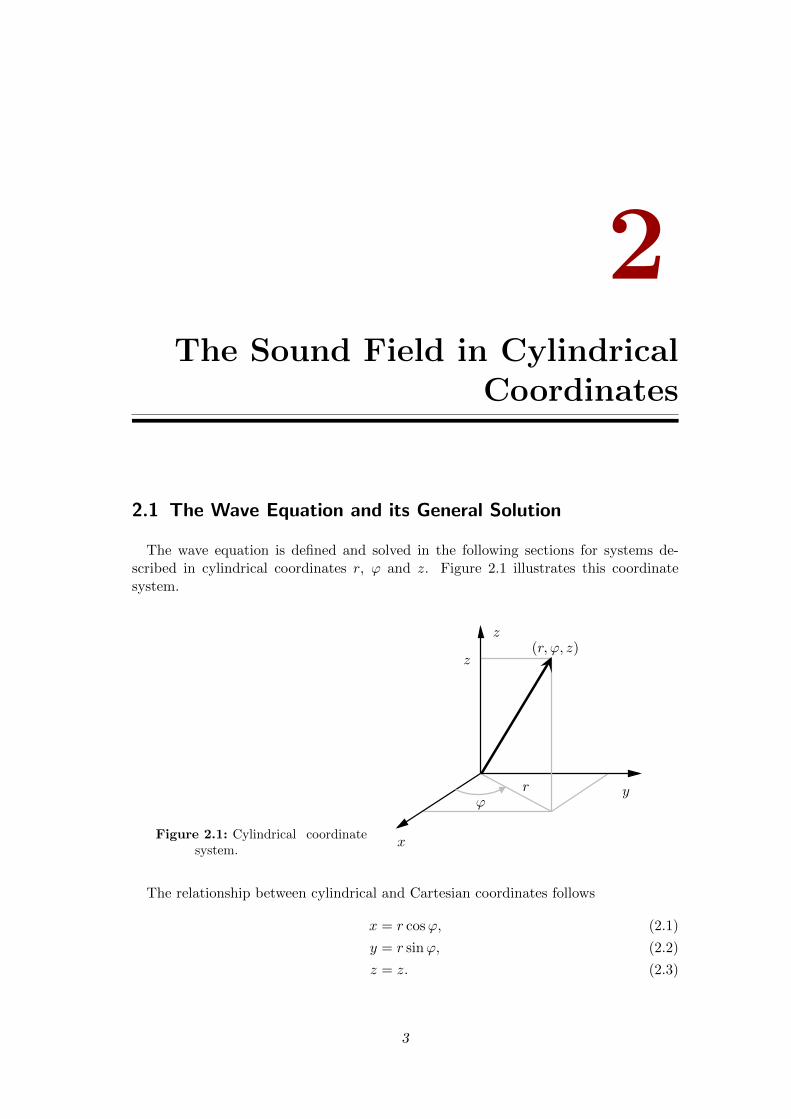
The wave equation is defined and solved in the following sections for systems de-scribed in cylindrical coordinates r, ' and z. Figure 2.1 illustrates this coordinatesystem.
Figure 2.1: Cylindrical coordinatesystem.
x
y
z
'r
z(r, ', z)
The relationship between cylindrical and Cartesian coordinates follows
x = r cos', (2.1)
y = r sin', (2.2)
z = z. (2.3)
3

4 Chapter 2 The Sound Field in Cylindrical Coordinates
2.1.1 The Wave Equation
The acoustical wave equation describes the variation of sound pressure p with timeand space as follows
∇2p− 1
c2∂2p
∂t2= 0, (2.4)
where c is the speed of sound and ∇2 is the Laplace operator which in cylindricalcoordinates is given by
∇2 =∂2
∂r2+
1
r
∂
∂r+
1
r2∂2
∂'2+
∂2
∂z2. (2.5)
The definition given for the wave equation is valid when the sound field behaves linearly[10]. When the sound pressure varies harmonically (i. e. sinusoidally) with time andfrequency at all positions, it is possible to represent the sound field using complexnotation. The complex pressure p can be defined as
p = ∣p∣ e−j(!t+�), (2.6)
where ! is the angular frequency and � is the phase of the complex sound pressure att = 0. The time dependence is represented by the factor −j!t. The sound pressure pis then obtained with the real part of p
p = Re {p} = Re{∣p∣ e−j(!t+�)
}= ∣p∣ cos(!t+ �). (2.7)
The use of complex notation is convenient as it simplifies the calculation when solvingthe wave equation.
The wave equation written using the complex pressure is
∇2p+(!c
)2p = 0. (2.8)
This equation is called the Helmholtz equation, and is usually expressed as follows
∇2p+ k2p = 0, (2.9)
where k is the wavenumber,
k =!
c. (2.10)
2.1.2 General Solution
In order to solve the Helmholtz equation, it is assumed that the complex pressure isa product of independent functions that depend on one single variable
p = p(r, ', z, t) = pr(r)p'(')pz(z)︸ ︷︷ ︸p(r,',z)
e−j!t, (2.11)

2.1 The Wave Equation and its General Solution 5
where the spatial terms can be distinguished from the temporal term
p(r, ', z, t) = p(r, ', z)e−j!t. (2.12)
Inserting the latter expression into the Helmholtz equation, it is revealed that thesolution only depends on the spatial term
∇2p(r, ', z) + k2p(r, ', z) = 0 (2.13)
The latter equation results, after inserting equation (2.11), in
p'(')pz(z)
(∂2pr(r)
∂r2+
1
r
∂pr(r)
∂r
)+
1
r2pr(r)pz(z)
∂2p'(')
∂'2
+ pr(r)p'(')∂2pz(z)
∂z2+ k2pr(r)p'(')pz(z) = 0, (2.14)
Dividing equation (2.14) by the term pr(r)p'(')pz(z) yields
1
pr(r)
(∂2pr(r)
∂r2+
1
r
∂pr(r)
∂r
)+
1
r21
p'(')
∂2p'∂'2
+1
pz(z)
∂2pz(z)
∂z2+ k2 = 0. (2.15)
The third term of the latter equation only depends on z and equals a sum of terms thatare independent of z
1
pz(z)
∂2pz(z)
∂z2= − 1
pr(r)
(∂2pr(r)
∂r2+
1
r
∂pr(r)
∂r
)− 1
r21
p'(')
∂2p'∂'2
− k2, (2.16)
which leads to the conclusion that this term must be a constant −k2z . Then,
1
pz(z)
d2pz(z)
dz2+ k2z = 0. (2.17)
Multiplying with the term r2, equation (2.15) can now be rewritten as
r2
pr(r)
∂2pr(r)
∂r2+
r
pr(r)
∂pr(r)
∂r+
1
p'(')
∂2p'∂'2
+ r2(k2 − k2z
)= 0. (2.18)
This equation reveals that the third term only depends on the ' coordinate and equalsa sum of terms that are independent. Using the same argumentation that in the caseof pz in equations (2.16) and (2.17), it is shown that
1
p'(')
d2p'(')
d'2+ k2' = 0, (2.19)
where −k2' is a constant. Using this value, equation (2.18) results in
r2
pr(r)
∂2pr(r)
∂r2+
r
pr(r)
∂pr(r)
∂r+ r2
(k2 − k2z −
k2'r2
)= 0. (2.20)
6 Chapter 2 The Sound Field in Cylindrical Coordinates
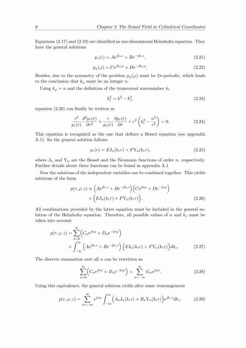
Equations (2.17) and (2.19) are identified as one-dimensional Helmholtz equation. Theyhave the general solutions
pz(z) = Ae jkzz +Be−jkzz, (2.21)
p'(') = Ce jk'' +De−jk''. (2.22)
Besides, due to the symmetry of the problem p'(') must be 2�-periodic, which leadsto the conclusion that k' must be an integer n.
Using k' = n and the definition of the transversal wavenumber kr
k2r = k2 − k2z , (2.23)
equation (2.20) can finally be written as
r2
pr(r)
∂2pr(r)
∂r2+
r
pr(r)
∂pr(r)
∂r+ r2
(k2r −
n2
r2
)= 0. (2.24)
This equation is recognized as the one that defines a Bessel equation (see appendixA.1). Its the general solution follows
pr(r) = EJn(krr) + FYn(krr), (2.25)
where Jn and Yn are the Bessel and the Neumann functions of order n, respectively.Further details about these functions can be found in appendix A.1
Now the solutions of the independent variables can be combined together. This yieldssolutions of the form
p(r, ', z) ∝(Ae jkzz +Be−jkzz
)(Ce jn' +De−jn'
)×(EJn(krr) + FYn(krr)
). (2.26)
All combinations provided by the latter equation must be included in the general so-lution of the Helmholtz equation. Therefore, all possible values of n and kz must betaken into account
p(r, ', z) =∞∑n=0
(Cne jn' +Dne−jn'
)×∫ ∞−∞
(Ae jkzz +Be−jkzz
)(EJn(krr) + FYn(krr)
)dkz. (2.27)
The discrete summation over all n can be rewritten as
∞∑n=0
(Cne jn' +Dne−jn'
)=
∞∑n=−∞
Gne jn'. (2.28)
Using this equivalence, the general solution yields after some rearrangement
p(r, ', z) =
∞∑n=−∞
e jn'
∫ ∞−∞
(AnJn(krr) +BnYn(krr)
)e jkzzdkz. (2.29)

2.1 The Wave Equation and its General Solution 7
Alternatively, the general solution can be given using Hankel functions
p(r, ', z) =
∞∑n=−∞
e jn'
∫ ∞−∞
(CnH(1)
n (krr) +DnH(2)n (krr)
)e jkzzdkz, (2.30)
where H(1)n and H
(2)n are the Hankel functions of first and second kind and order n,
respectively. These are defined as follows
H(1)n (x) = Jn(x) + jYn(x), (2.31)
H(2)n (x) = Jn(x)− jYn(x). (2.32)
The values An, Bn, Cn and Dn in the equations of the general solution are determinedby means of the boundary conditions of the problem under analysis. Of special interestare the interior and the exterior problems described in the following section.
2.1.3 Interior and Exterior Boundary Value Problems
The interior and the exterior boundary value problem are characterized by both theregion where the wave equation is valid and the location of the sound sources withrespect to the region of validity. A sketch of these problems is shown in figure 2.2.
Source
Region ofvalidity
surfaceBoundary
(a) Interior problem.
Source
validityRegion of
surfaceBoundary
(b) Exterior problem.
Figure 2.2: Interior and exterior problems. The region of validity of the wave equation isrepresented by the gray area.
These two boundary problems are described as follows
� Interior problems. The sources are located completely outside the boundarysurface, which is the limit of the region of validity. This implies that the soundpressure must be finite at the origin. This behavior is not easily described bymeans of equation (2.30) since the Hankel functions are infinite at the origin.Therefore, equation (2.29) must be used instead. Whereas the term Jn is finite atthe origin, the term Yn is infinite as can be seen in figure A.1 in appendix A.1. Asa consequence, Bn must be set to zero. In this case, the general solution simplifies

8 Chapter 2 The Sound Field in Cylindrical Coordinates
to
p(r, ', z) =∞∑
n=−∞e jn'
∫ ∞−∞
AnJn(krr)ejkzzdkz. (2.33)
This boundary problem is the case, for example, of the sound field inside a cylin-drical duct [10].
� Exterior problems. In this case, the boundary surface totally encloses all thesources. Now, equation (2.30) is used as the condition for a finite field at theorigin is no longer valid.
The boundary condition at infinity, is in this case given by the Sommerfeld ra-diation condition1 which states that only outgoing waves can exist [12]. Theasymptotic behavior of the Hankel functions for large arguments, i. e. at r →∞,follows
limr→∞
H(1)n (krr) =
√2
�krre j(krr−n�/2−�/4), (2.34)
limr→∞
H(2)n (krr) =
√2
�krre−j(krr−n�/2−�/4). (2.35)
Using the convention e−j!t, it becomes obvious that equation (2.34) representsoutgoing waves, whereas equation (2.35) represents incoming waves [13]. There-fore, to fulfill the Sommerfeld condition it must be imposed that Dn = 0, and thesolution of the wave equation becomes
p(r, ', z) =∞∑
n=−∞e jn'
∫ ∞−∞
CnH(1)n (krr)e
jkzzdkz. (2.36)
The exterior problem is of interest when dealing with scattering from rigid cylin-ders, as will be seen in the following section.
2.2 Scattering from Rigid Cylinders
When a sound wave encounters an obstacle, some of the wave is deflected from itsoriginal path. For linear problems, the difference between the actual sound field andthe sound field that would be present if the obstacle was not there is the scattered wave.Hence, the total pressure can be written as the sum of the incident and the scatteredpressure,
ptotal = pi + psc. (2.37)
In this section it is considered that the incoming waves are created by a point sourcein the far-field, which implies that the waves that interact with the obstacle can beregarded as plane waves [14]. The obstacle that creates scattering is assumed to be acylinder with a rigid surface. Due to the stiffness, the total radial particle velocity atthe surface of the cylinder must be zero.
1The Sommerfeld radiation condition is given in detail in [11] for spherical waves.

2.2 Scattering from Rigid Cylinders 9
In addition, it is also assumed that the vibration of the cylindrical surface is indepen-dent of the axial coordinate. This assumption corresponds to a symmetric setup thatsimplifies further derivations, and in effect, reduces the problem to two dimensions.
The scattering from cylinders is here described for cylinders of finite and infinitelength. The geometry of the problem, depicted in figure 2.3, shows an incident wave,characterized by a plane wave moving along the direction of the wavenumber ki, thatis obstructed by a cylinder of radius R and length 2L. Note that cylinders of infinitelength are represented when L→∞.
z
x
y
L
−L
ki
'i
cylinder
'
Rigid
r Q
R
Figure 2.3: Geometrical model considered for the scattering problem. The incident wavesimpinge on a rigid cylinder of radius R and length 2L.
2.2.1 Cylindrical Scatterer of Infinite Length
Consider a plane wave created by a source that travels perpendicularly to the axisof the cylinder, i. e. perpendicular to the z-axis. In the absence of the cylinder, theincident wave traveling in the direction ki is, at a point Q(r, '),
pi(r) = P0ej(ki · r−!t), (2.38)
where P0 is the amplitude of the plane wave and r is the position vector in a cylindricalcoordinate system. For mathematical simplicity, and due to the symmetry of the prob-lem, the z-coordinate of the vectors ki and r is set to zero. In Cartesian coordinatesthe wavenumber vector ki is
ki = k (cos'iex + sin'iey + 0ez) , (2.39)
where 'i is the angle of incidence of the plane wave in the xy-plane (see figure 2.3) andex, ey and ez represent the unit vectors along the x, y and z-axis, respectively. The

10 Chapter 2 The Sound Field in Cylindrical Coordinates
position vector r is, in Cartesian coordinates,
r = r (cos'ex + sin'ey + 0ez) . (2.40)
Now, using the previous expressions in Cartesian coordinates, the pressure of theincident wave becomes
pi(r, ', t) = P0ej(kr(cos'i cos'+sin'i sin')−!t
)= P0e
j(kr cos('−'i)−!t
). (2.41)
As the incident plane wave is created far from the cylinder and approaches the cylinderplaced at the origin, the situation can be regarded as an interior boundary problemaccording to section 2.1.3. Therefore, the sound field created by the incident wavemust be expressible in terms of equation (2.33). Taking into account that the planewave travels perpendicularly to the z-axis, kz must be zero meaning that k = kr (seeequation (2.23)). Going back to section 2.1.2, the particular solution for pz(z) given inequation (2.21) is reduced to a constant since kz = 0. This implies that the generalsolution does not present the integral with respect to kz. As a consequence, the pressurein the case of the interior boundary problem becomes
pi(r, ', t) = e−j!t∞∑
n=−∞e jn'AnJn(kr). (2.42)
Note that in the latter equation the pressure is expressed in complex notation so thetemporal term must be present. Equation (2.41) must equal equation (2.42)
P0ej(kr cos('−'i)−!t
)= e−j!t
∞∑n=−∞
e jn'AnJn(kr). (2.43)
The coefficients An are obtained by multiplying both sides of the latter equation withe−j�' and integrating over '∫ 2�
0e−j�'P0e
jkr cos('−'i)d' =
∫ 2�
0e−j�'
∞∑n=−∞
e jn'AnJn(kr)d', (2.44)
then,
P0
∫ 2�
0e jkr cos('−'i)e−j�'d' =
∞∑n=−∞
AnJn(kr)
∫ 2�
0e−j�'e jn'd'. (2.45)
The functions of the form e jn' are orthogonal, which implies that the integral of theright side term equals 0 when n ∕= � or 2� when n = �. More details about thesefunctions are given in section 3.1. Therefore, equation (2.45) is simplified to
P0
∫ 2�
0e j(kr cos('−'i)−n'
)d' = 2�AnJn(kr). (2.46)

2.2 Scattering from Rigid Cylinders 11
Applying the change of variables = '−'i at the left side term of the latter equationyields
P0e−jn'i
∫ 2�
0e j(kr cos −n )d = 2�AnJn(kr). (2.47)
According to equation (A.4) given in appendix A.1, the integral at the left side of theprevious equation equals∫ 2�
0e j(kr cos −n )d = 2�(j)−nJ−n(kr). (2.48)
Using the property found in the previous equation and the relationship between J−nand Jn given in equation (A.6), the coefficients An can be isolated from equation (2.47)
An = P0jne−jn'i . (2.49)
Finally, inserting this value into equation (2.42), the incident pressure is given by
pi(r, ', t) = P0e−j!t
∞∑n=−∞
jnJn(kr)e jn('−'i). (2.50)
As mentioned previously, the radial velocity vanishes on the surface of a rigid cylinderat r = R
utotal,r(R,', t) = ui,r(R,', t) + usc,r(R,', t) = 0. (2.51)
Therefore, usc,r(R,', t) = −ui,r(R,', t). The particle velocity in the radial directiondue to the incoming wave is
ui,r(R,', t) =1
j!�0
dpi(r, ', t)
dr
∣∣∣∣r=R
=P0e
−j!t
j!�0
∞∑n=−∞
jndJn(kr)
dre jn('−'i)
∣∣∣∣∣r=R
, (2.52)
where �0 is the equilibrium density of the medium. The scattered pressure can beregarded as an exterior boundary problem, and consequently it can be written by thesum of outgoing waves described in equation (2.36). However, the integral with respectto kz can be removed from the equation due to the fact that it has been assumed thatthe vibration of the cylindrical surface is independent of the axial coordinate. Similarlyto the derivation of pi, this implies that kz = 0, hence the solution of pz(z) yields aconstant (see equation (2.21)), and the general solution does not depend on kz. Thescattered pressure is then
psc(r, ', t) = e−j!t∞∑
n=−∞e jn'CnH(1)
n (kr). (2.53)
The scattered particle velocity in the radial direction is given by
usc,r(r, ', t) =1
j!�0
dpsc(r, ')
dr=
e−j!t
j!�0
∞∑n=−∞
e jn'CndH
(1)n (kr)
dr. (2.54)

12 Chapter 2 The Sound Field in Cylindrical Coordinates
Equation (2.52) can be related to the latter expression evaluated at r = R, accordingto equation (2.51),
e−j!t∞∑
n=−∞e jn'CnH′(1)n (kR) = −P0e
−j!t∞∑
n=−∞jnJ′n(kR)e jn('−'i), (2.55)
where J′n(kR) and H′(1)n (kR) are given by
J′n(kR) =dJn(kr)
dr
∣∣∣∣r=R
, (2.56)
H′(1)n (kR) =dH
(1)n (kr)
dr
∣∣∣∣∣r=R
. (2.57)
Now, the coefficients Cn can be isolated from equation (2.55)
Cn = −P0jn J′n(kR)
H′(1)n (kR)
e−jn'i . (2.58)
Making use of Cn, the scattered pressure and the total pressure result in
psc(r, ', t) = −P0e−j!t
∞∑n=−∞
jnJ′n(kR)H
(1)n (kr)
H′(1)n (kR)
e jn('−'i), (2.59)
and
ptotal(r, ', t) = P0e−j!t
∞∑n=−∞
jn
(Jn(kr)− J′n(kR)H
(1)n (kr)
H′(1)n (kR)
)e jn('−'i). (2.60)
Of special interest will be the sound field on the surface of the cylinder of infinitelength
ptotal(R,', t) = P0e−j!t
∞∑n=−∞
jn
(Jn(kR)− J′n(kR)H
(1)n (kR)
H′(1)n (kR)
)e jn('−'i). (2.61)
2.2.2 Cylindrical Scatterer of Finite Length
The total sound field when a cylinder of finite length is present is usually difficultto solve analytically. As in the case of the infinite-length cylinder, an incident planewave with amplitude P0 traveling in the direction ki is assumed (see equation (2.38)).This impinges on the finite-length rigid scatterer orthogonally to the cylindrical axis.Therefore, the expression of the incident pressure derived for the case of an infinitelylong cylinder (given in equation (2.50)) is still valid.
2.2 Scattering from Rigid Cylinders 13
Neglecting the boundary conditions at the end caps of the cylinder (at z = L andz = −L), the following approximation for the scattered sound pressure2 is given in [15]
psc(r, ', z, t) = −P0e−j!tkL
�
∞∑n=−∞
jnJ′n(kR)e jn('−'i)
×∫ ∞−∞
H(1)n (√k2 − k2zr)sinc(kzL)√
k2 − k2zH′(1)n (
√k2 − k2zR)
e jkzzdkz, (2.62)
where the sinc function is defined as
sinc(kzL) =sin(kzL)
kzL. (2.63)
The scattered pressure due to a cylinder of infinite length can be derived from thefinite-length cylinder case. At L → ∞, only the term Lsinc(kzL) of equation (2.62) isaffected. Using the relationship [16]
�(kz) = limL→∞
1
�kzsin(kzL), (2.64)
the upper limit of the term Lsinc(kzL) follows
limL→∞
Lsinc(kzL) = limL→∞
sin(kzL)
kz= lim
L→∞
�
�kzsin(kzL) = ��(kz). (2.65)
The result of inserting the latter relation into equation (2.62) is the same as the oneobtained for the infinite-length cylinder in equation (2.59).
The total sound pressure, given by the summation of the incident and the scatteredpressures, is
ptotal(r, ', z, t) = P0
∞∑n=−∞
jne jn('−'i)
(Jn(kr)− kL
�J′n(kR)
×∫ ∞−∞
H(1)n (√k2 − k2zr)sinc(kzL)√
k2 − k2zH′(1)n (
√k2 − k2zR)
e jkzzdkz
)e−j!t. (2.66)
Of special importance will be the pressure on the surface of a rigid cylinder of finitelength in the xy-plane, i. e. at z = 0
ptotal(R,', t) = P0
∞∑n=−∞
jne jn('−'i)
(Jn(kR)− kL
�J′n(kR)
×∫ ∞−∞
H(1)n (√k2 − k2zR)sinc(kzL)√
k2 − k2zH′(1)n (
√k2 − k2zR)
dkz
)e−j!t. (2.67)
2The derivation of the scattered sound pressure from a finite cylinder is beyond the scope of thisdocument. Details about it are given in [15].


3Sound Field Decomposition
3.1 Fourier Series
The decomposition of a function in a Fourier Series is of great utility when dealingwith functions that present circular symmetry. A function defined in polar coordinates(r and ') can be represented in a Fourier series in the ' coordinate as [17]
f(r, ') =
∞∑n=−∞
Cn(r)e jn', (3.1)
where the coefficient functions Cn(r) are given by
Cn(r) =1
2�
∫ 2�
0f(r, ')e−jn'd'. (3.2)
The representation in terms of Fourier series is in fact a summation modes of the form
fn(r, ') = Cn(r)e jn'. (3.3)
The terms e jn' are referred to as circular harmonics (CH). In the literature, othernames can be found, e. g. circumferential harmonics. Figure 3.1 shows the magnitudeof the real part of the first six harmonics,
∣∣Re{
e jn'}∣∣, as a function of '. As can be
seen, these harmonics correspond to multipoles: order 0 yields a monopole, order 1 adipole, etc. An important property of the CH is that they are orthogonal, which meansthat they satisfy
1
2�
∫ 2�
0e jn'(e j�')∗d' = �n� , (3.4)
where �n� is the Kronecker function which equals unity when n = � and it is zerootherwise.
15

16 Chapter 3 Sound Field Decomposition
0∘
45∘
90∘
135∘
180∘
225∘
270∘
315∘
(a) n = 0
0∘
45∘
90∘
135∘
180∘
225∘
270∘
315∘
(b) n = 1
0∘
45∘
90∘
135∘
180∘
225∘
270∘
315∘
(c) n = 2
0∘
45∘
90∘
135∘
180∘
225∘
270∘
315∘
(d) n = 3
0∘
45∘
90∘
135∘
180∘
225∘
270∘
315∘
(e) n = 4
0∘
45∘
90∘
135∘
180∘
225∘
270∘
315∘
(f) n = 5
Figure 3.1: Magnitude of the real part of the CH as a function of ', for the first sixorders. The outer circle corresponds to a level of 0 dB.
3.2 Sound Field Decomposition using Circular Apertures
In this section the sound field captured by a circular aperture is decomposed in aFourier series, and its modal response is analyzed in two configurations. The first one,namely the unbaffled case, consists of a circular aperture that is not mounted on anybaffle. For the second setup, the aperture is mounted on a rigid cylindrical baffle andis referred to as a baffled circular aperture.
3.2.1 Unbaffled Circular Apertures
In the following, the modal properties of an unbaffled circular array are analyzed.As shown in figure 3.2, a circular aperture of radius R that lies on the xy-plane isconsidered as well as a plane wave that impinges on the aperture perpendicularly tothe z-axis. The aperture is not regarded as an obstacle by the impinging wave, andtherefore, the pressure on the aperture is only due to the wave itself. In other words,no scattered sound field is created. The incident pressure at any point of the apertureis, according to equation (2.50) on page 11,
p(kR, ') = P0ejki · r
∣∣∣r=R
= P0
∞∑n=−∞
jnJn(kR)e jn('−'i), (3.5)
where the product of the wavenumber k and the radius of th aperture R, i. e. kR, isreferred to as spatial frequency. Note that the temporal term e−j!t is not shown in

3.2 Sound Field Decomposition using Circular Apertures 17
z
x
y
R
ki
'i
'
apertureCircular
Figure 3.2: Plane wave impinging on a circular aperture.
the latter equation in order to simplify following derivations. The pressure can nowbe decomposed by an infinite number of modes (harmonics) using the principles of theFourier series given in equations (3.1) and (3.2)
p(kR, ') =∞∑
n=−∞C∘n(kR)e jn', (3.6)
C∘n(kR) =1
2�
∫ 2�
0p(kR, ')e−jn'd'. (3.7)
The superscript ∘ in the coefficient functions denotes that an unbaffled circular apertureis under consideration. The coefficients C∘n are found after inserting equation (3.5) intoequation (3.7)
C∘n(kR) =1
2�
∫ 2�
0P0
∞∑�=−∞
j�J�(kR)e j�('−'i)e−jn'd'. (3.8)
Due to the fact that the CH are orthogonal, as stated previously in equation (3.4), thecoefficients result in
C∘n(kR) = P0jnJn(kR)e−jn'i . (3.9)
The magnitude of the first five coefficients C∘n is shown in figure 3.3. At low spatialfrequencies kR, the zeroth order mode is constant and equals 0 dB, whereas all theother modes present a slope of 10× n dB per decade. This means that the zerothorder is the order that has more strength in this range of spatial frequencies. With theincrease of kR more and more harmonics gain strength, but around some values theypresent dips. The consequence is that signals that have components around these dipscannot be totally resolved. As shown in the next section, this problem can be solvedby mounting the aperture on a rigid scatterer. Due to the geometry of the aperture,the scatterer should be a rigid cylindrical baffle.

18 Chapter 3 Sound Field Decomposition
kR
Magnitudeof
C∘ n[dB]
n = 0n = 1n = 2n = 3n = 4
10−1 100 101−150
−100
−50
0
Figure 3.3: Magnitude of the Fourier coefficients of an unbaffled circular aperture, C∘n,when P0 = 1 Pa. The first five modes are shown.
3.2.2 Circular Apertures Mounted on a Rigid Cylindrical Baffle
It is considered that the aperture of the previous section is now mounted on a rigidcylindrical baffle as can be seen in figure 3.4. The assumptions made for the unbaffledaperture regarding the features of the impinging wave are still valid. However, now thepresence of the cylinder causes scattering. The theory given for cylindrical scatterers insection 2.2.2 is therefore of great utility in this section. The modal response the baffledapertures is analyzed for cylindrical scatterers of finite and infinite length.
3.2.2.1 Baffle of Infinite Length
The pressure captured by an aperture mounted on a rigid cylindrical baffle of infinitelength corresponds to the pressure on the surface of a rigid cylindrical scatterer ofinfinite length derived in section 2.2.1. The modal response such aperture is obtainedby means of the pressure given in equation (2.61) on page 12
C�n(kR) =1
2�
∫ 2�
0P0
∞∑n=−∞
j�
(J�(kR)− J′�(kR)H
(1)� (kR)
H′(1)� (kR)
)e j�('−'i)e−jn'd'. (3.10)
The superscript � denotes that the aperture is mounted on a cylindrical baffle of infinitelength. Due to the orthogonality property of the CH, the coefficients result in
C�n(kR) = P0jn
(Jn(kR)− J′n(kR)H
(1)n (kR)
H′(1)n (kR)
)e−jn'i . (3.11)
In figure 3.5, the magnitude of the first five Fourier coefficients C�n is shown. At firstsight, one can see that at low spatial frequencies the response is rather similar to the

3.2 Sound Field Decomposition using Circular Apertures 19
z
x
y
L
−L
R
ki
'i
baffle
'
Rigid
apertureCircular
Figure 3.4: Circular aperture of radius R mounted on a cylindrical baffle of the sameradius and length 2L.
kR
Magnitudeof
C∙ n[dB]
n = 0n = 1n = 2n = 3n = 4
10−1 100 101−150
−100
−50
0
Figure 3.5: Magnitude of the Fourier coefficients of a circular aperture mounted on a rigidcylindrical baffle of infinite length, C�n, when P0 = 1 Pa. The first five modes areshown.

20 Chapter 3 Sound Field Decomposition
one of the unbaffled aperture since the slope of 10× n dB per decade is also present,see figure 3.3. The only difference is that the response is offset by 6 dB with respect tothe unbaffled aperture response. This offset is caused by the stiffness of the cylinder.As its impedance is high, the radial particle velocity is canceled and the sound pressureis doubled. On the other hand, at high values of kR the problem presented for theunbaffled aperture is totally solved, i. e. the dips are canceled, and all the spatial fre-quencies can be successfully resolved. Furthermore, at these frequencies all the modespresent the same response, which means that all of them have the same strength.
3.2.2.2 Baffle of Finite Length
Obviously, for real implementations it is not possible to use cylindrical baffles ofinfinite length, and hence, finite-length scatterers with a reasonable length must beused instead. The pressure on the surface of a cylindrical scatterer of finite length hasbeen given in section 2.2.2. The pressure that an aperture captures when it is mountedon this scatterer at z = 0 (given in equation (2.67) on page 2.67) is decomposed in CHas follows
CLn (kR) =1
2�
∫ 2�
0P0
∞∑�=−∞
j�
(Jn(kR)− kL
�J′�(kR)
×∫ ∞−∞
H(1)� (√k2 − k2zR)sinc(kzL)√
k2 − k2zH′(1)� (
√k2 − k2zR)
dkz
)e j�('−'i)e−jn'd'. (3.12)
In the coefficients CLn the superscript ‘L’ denotes that the baffle has a finite length.After solving the integral with respect to ', the coefficients yield
CLn (kR) =P0jn
(Jn(kR)− kL
�J′n(kR)
×∫ ∞−∞
H(1)n (√k2 − k2zR)sinc(kzL)√
k2 − k2zH′(1)n (
√k2 − k2zR)
dkz
)e−jn'i . (3.13)
In figure 3.6, the magnitude of the first four modes is shown for various ratios ofL/R. These results were presented by Teutsch in [9] and [15]. The unbaffled case isrepresented when L/R = 0 and the infinite baffle case, when L/R =∞. At low spatialfrequencies all curves in all the panels of the figure are parallel, presenting a slope of10× n dB per decade independently of the ratio L/R. Note that the difference of 6 dBin offset between the infinite baffle and the unbaffled cases becomes clear. For verysmall ratios, dips are still present at high values of kR but they vanish progressivelywhen the ratio increases due to the fact that the response becomes more similar to theone obtained with the infinite baffle. Teutsch concludes that with a ratio of 1.4 themodal response is fairly similar to the one of the infinite baffle case. This is a veryconvenient result for a real implementation of the system, because for ratios L/R > 1.4the coefficients CLn can be approximated to the expression presented for the infinite-length baffle in equation (3.11), which agrees in high level with the actual result and iscomputationally simpler.
To verify Teutsch results, the modal response for a baffle of finite length has been

3.2 Sound Field Decomposition using Circular Apertures 21
Figure 3.6: Magnitude of the Fourier coefficients of a circular aperture mounted on a rigidcylindrical baffle of finite length. The first four modes are shown for different valuesof L/R. Taken from [15].
implemented. The results, shown in figure 3.7, reveal significant differences from hisresults. Comparing the two sets of results, it can be seen that the modal response forthe unbaffled aperture and for the aperture mounted on an infinitely-long baffle agreewith Teutsch results shown in figure 3.6, in all the spatial frequency range. However,the results deviate when dealing with finite baffles. The obtained curves present a slopeat low values of kR that differs of 10× n dB per decade, which was the value obtainedby Teutsch. At higher frequencies, the differences also become apparent, mostly forL/R = 1.4. Unlike Teutsch results, this curve is not that similar to the one obtained inthe infinite baffle case, as some boosts and dips are now present. Therefore, in this case,one cannot say that with a ratio of L/R = 1.4 the aperture can be considered to bemounted into an infinite baffle.1 Even though it is not shown here, the curves only getcloser to the case of the infinite baffle for rather high ratios of L/R (around L/R ≈ 20).The Matlab scripts implemented for the aperture mounted on a finite baffle are givenin appendix B.1
1Teutsch was contacted during the realization of this project in order to find out the reason for thedifference in the results. However, no solution came out from the correspondence.

22 Chapter 3 Sound Field Decomposition
Magnit
ude
[dB
]
kR
10−1 100 101
−100
−80
−60
−40
−20
0
(a) n = 0
Magnit
ude
[dB
]
kR
L/R = 0
L/R = 0.1
L/R = 1.4
L/R = ∞
10−1 100 101
−100
−80
−60
−40
−20
0
(b) n = 1
Magnit
ude
[dB
]
kR
10−1 100 101
−100
−80
−60
−40
−20
0
(c) n = 2
Magnit
ude
[dB
]
kR
10−1 100 101
−100
−80
−60
−40
−20
0
(d) n = 3
Figure 3.7: Magnitude of the Fourier coefficients of a circular aperture when P0 = 1 Pa.The first four modes are shown for the values of L/R stated in panel (b). Note thatL/R = 0 corresponds to an unbaffled aperture, L/R =∞ is the case of an aperturemounted on a baffle of infinite length, whereas the cases where the aperture ismounted on a baffle of finite length are represented by L/R equal to 0.1 and 1.4.The latter two cases, i. e. when the aperture is mounted on a baffle of finite length,are obtained with the Matlab scripts given in appendix B.1.
3.3 Error due to Truncation
The sound field can be decomposed in CH, where the superposition of all the modesyields the sound field under analysis. However, in practice, only a certain number ofharmonics can be used, and therefore, the sound field is approximated by
p(kR, ') ≈N∑
n=−NCn(kR)e jn', (3.14)

3.3 Error due to Truncation 23
where N is the maximum order. As a consequence, the so-called truncation error arises.In the case of unbaffled circular apertures, this error is
ℰ�t,n(kR) =
∞∑n=−∞
jnJn(kR)e jn('−'i) −N∑
n=−NjnJn(kR)e jn('−'i)
=∑∣n∣>N
jnJn(kR)e jn('−'i). (3.15)
By analogy, the expression for circular apertures mounted on a rigid cylindrical baffleof infinite length is obtained
ℰ�t,n(kR) =
∞∑n=−∞
jn(
Jn(kR)− J′n(kR)Hn(kR)
H′n(kR)
)e jn('−'i)
−N∑
n=−Njn(
Jn(kR)− J′n(kR)Hn(kR)
H′n(kR)
)e jn('−'i)
=∑∣n∣>N
jn(
Jn(kR)− J′n(kR)Hn(kR)
H′n(kR)
)e jn('−'i). (3.16)
According to [15], the mean square truncation error of an unbaffled circular aperturefollows
ℰ2�t,n =1
2�
∫ 2�
0
∣∣∣∣∣∣∑∣n∣>N
jnJn(kR)e jn('−'i)
∣∣∣∣∣∣2
d' = 2 ·
∞∑n=N+1
J2n(kR). (3.17)
For a circular aperture mounted on a cylindrical baffle of infinite length, it is given by
ℰ2�t,n =1
2�
∫ 2�
0
∣∣∣∣∣∣∑∣n∣>N
jn(
Jn(kR)− J′n(kR)Hn(kR)
H′n(kR)
)e jn('−'i)
∣∣∣∣∣∣2
d'
= 2 ·
∞∑n=N+1
(Jn(kR)− J′n(kR)Hn(kR)
H′n(kR)
)2
. (3.18)
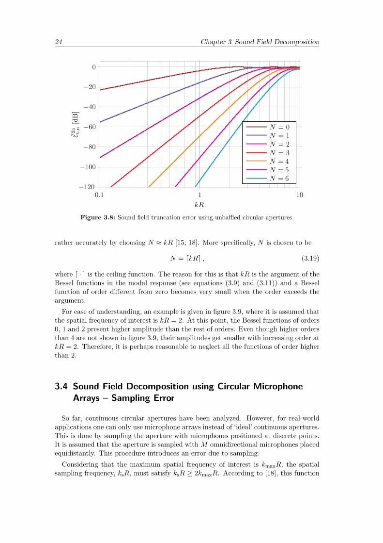
Figure 3.8 shows the magnitude of the truncation error for unbaffled circular aper-tures. As can be seen, at low spatial frequencies each order presents smaller error thanat high frequencies. Besides, at low spatial frequencies the error is reduced when thenumber of orders taken into account increases. However, at the highest frequencies thetruncation error becomes similar independently of the number of orders that are used.
For a fixed error, the results reveal that for low spatial frequencies a small number oforders can be used, whereas with increasing kR the number of orders used to achievethe same error has to be increased. This means that the sound field can be representedrather accurately with few harmonics at low spatial frequencies, whereas to represent itwith the same accuracy at higher frequencies, the maximum order of harmonics needsto be increased.
According to the previous reasoning, it turns out that the sound field can be described
24 Chapter 3 Sound Field Decomposition
kR
ℰ2∘
t,n
[dB]
N = 0N = 1N = 2N = 3N = 4N = 5N = 6
0.1 1 10−120
−100
−80
−60
−40
−20
0
Figure 3.8: Sound field truncation error using unbaffled circular apertures.
rather accurately by choosing N ≈ kR [15, 18]. More specifically, N is chosen to be
N = ⌈kR⌉ , (3.19)
where ⌈ · ⌉ is the ceiling function. The reason for this is that kR is the argument of theBessel functions in the modal response (see equations (3.9) and (3.11)) and a Besselfunction of order different from zero becomes very small when the order exceeds theargument.
For ease of understanding, an example is given in figure 3.9, where it is assumed thatthe spatial frequency of interest is kR = 2. At this point, the Bessel functions of orders0, 1 and 2 present higher amplitude than the rest of orders. Even though higher ordersthan 4 are not shown in figure 3.9, their amplitudes get smaller with increasing order atkR = 2. Therefore, it is perhaps reasonable to neglect all the functions of order higherthan 2.
3.4 Sound Field Decomposition using Circular MicrophoneArrays – Sampling Error
So far, continuous circular apertures have been analyzed. However, for real-worldapplications one can only use microphone arrays instead of ‘ideal’ continuous apertures.This is done by sampling the aperture with microphones positioned at discrete points.It is assumed that the aperture is sampled with M omnidirectional microphones placedequidistantly. This procedure introduces an error due to sampling.
Considering that the maximum spatial frequency of interest is kmaxR, the spatialsampling frequency, ksR, must satisfy ksR ≥ 2kmaxR. According to [18], this function

3.4 Sound Field Decomposition using Circular Microphone Arrays – Sampling Error25
kR
Jn
n = 0
n = 1
n = 2
n = 3
n = 4
0 1 2 3 4 5 6
−0.5
0
0.5
1
Figure 3.9: Magnitude of the Bessel functions, where the values at kR = 2 are highlightedwith a dot. Up to order 2, these functions present significant amplitude, whereasfor higher orders the amplitude can be neglected as it gets smaller.
is, in two-dimensions,
S(') =∞∑
p=−∞�('− p'si)
=1
'si
∞∑q=−∞
e jqM'
=1
'si
⎛⎝1 +
∞∑q=1
(e jqM' + e−jqM'
)⎞⎠ , (3.20)
where the sampling interval along the circle, 'si, is
'si =�
kmaxR. (3.21)
Applying the sampling function on the Fourier coefficients obtained with an unbaffledaperture (see equation (3.9)), the sampled coefficients become
C∘n(kR) = jnJn(kR)e−jn'i︸ ︷︷ ︸C∘n(kR)
+∞∑q=1
(jgJg(kR)e jg'i + jℎJℎ(kR)e−jℎ'i
)︸ ︷︷ ︸
C∘e,n(kR)
, (3.22)
where g = (Mq−n) and ℎ = (Mq+n). The tilde in C∘n is used to emphasize that thesecoefficients are approximated by using microphone arrays instead of apertures. Byanalyzing the sampled coefficients, one can see that the first term corresponds to the

26 Chapter 3 Sound Field Decomposition
coefficients of an unbaffled circular aperture C∘n, whereas the second term gives the errordue to sampling C∘e,n. The error, which is a series of Bessel functions, can be minimizedrecalling the idea that the Bessel functions become negligible when the order exceedsthe argument. In this sense, if the smallest order has a negligible amplitude, it can beensured that the rest of modes will have even smaller amplitude. This is satisfied whenthe smallest order, M − n (when q = 1), exceeds the maximum argument; that is
M − n > ⌈kmaxR⌉ . (3.23)
Since according to section 3.3, the maximum order should follow Nmax = ⌈kmaxR⌉ inorder to minimize the error due to truncation, n must be
n ≤ Nmax = ⌈kmaxR⌉ . (3.24)
Inserting the maximum value of n, i. e. n = Nmax = ⌈kmaxR⌉, into equation (3.23)yields
M −Nmax > ⌈kmaxR⌉ ⇔M − ⌈kmaxR⌉ > ⌈kmaxR⌉ ⇔
M > 2 ⌈kmaxR⌉ . (3.25)
In conclusion, the sampling error is minimized when the number of microphones follows
M > 2 ⌈kmaxR⌉ ⇔ M > 2Nmax. (3.26)
This condition is satisfied when the distance between microphones along the arc of thecircle is
darc =2�R
M⇔
M =2�R
darc> 2Nmax ⇔
darc <2�R
2Nmax=
2�R
2 ⌈kmaxR⌉⇔
darc <2�R
2kmaxR⇔
darc <�min
2. (3.27)
By analogy, the sampled coefficients obtained with a circular array mounted on baffle
3.4 Sound Field Decomposition using Circular Microphone Arrays – Sampling Error27
of infinite length are given by
C�n(kR) = jn(
Jn(kR)− J′n(kR)Hn(kR)
H′n(kR)
)e−jn'i
+∞∑q=1
jg(
Jg(kR)−J′g(kR)Hg(kR)
H′g(kR)
)e jg'i
+∞∑q=1
jℎ(
Jℎ(kR)− J′ℎ(kR)Hℎ(kR)
H′ℎ(kR)
)e−jℎ'i , (3.28)
where the first term corresponds to the Fourier coefficients of an aperture mounted onan infinite baffle, and the second and third terms are the error due to the samplingoperation,
C�e,n(kR) =∞∑q=1
jg(
Jg(kR)−J′g(kR)Hg(kR)
H′g(kR)
)e jg'i
+∞∑q=1
jℎ(
Jℎ(kR)− J′ℎ(kR)Hℎ(kR)
H′ℎ(kR)
)e−jℎ'i . (3.29)
In figure 3.11, the first six theoretical coefficients of an unbaffled aperture are com-pared to the approximated coefficients obtained with an unbaffled array of 12 micro-phones. As can be seen, the theoretical coefficients and the approximated ones areidentical, for each order, in almost the entire spatial frequency range. Just at thehigher values of kR, deviations between them are observed, which are caused by thesampling error. In fact, the error is present at a lower value of kR with increasingorder, which agrees with equation (3.23). Therefore, the most restrictive case is foundfor the highest order shown, n = 5, where the error appears at about kR = 5, seepanel (f). This is indeed what we expect from equation (3.26). In this equation themaximum value kR that can be represented without having sampling error is relatedto the number of microphones. In the present case, M is 12, then, ⌈kmaxR⌉ < 12/2,and hence kmaxR=5. According to equation (3.19), this also means that the sound fieldcan be represented very accurately up to order 5, i. e. Nmax = 5. In contrast with this,when the order of the coefficients exceeds Nmax, the approximated coefficients do notmatch the theoretical ones due to the sampling error. This is illustrated in figure 3.11,for n = 6 and n = 7.
To sum up, the sound field decomposed with a circular array of M microphones isvery similar to the decomposition that would be obtained with an aperture of the sameradius, up to a maximum spatial frequency ⌈kmaxR⌉ < M/2. Above this value, samplingerror occurs. Furthermore, the maximum order that can be represented accuratelyfollows Nmax = ⌈kmaxR⌉.
The foregoing ideas can also be examined by means of the relative error due to thesampling process. This is defined as [15]
ℰs,n(kR) =
∣∣∣∣Ce,n(kR)
Cn(kR)
∣∣∣∣2 . (3.30)

28 Chapter 3 Sound Field Decomposition
kR
Magnitude[dB]
C∘
n
C∘
n
0.1 1 10−80
−60
−40
−20
0
(a) n = 0
kR
Magnitude[dB]
0.1 1 10−80
−60
−40
−20
0
(b) n = 1
kR
Magnitude[dB]
0.1 1 10−80
−60
−40
−20
0
(c) n = 2
kR
Magnitude[dB]
0.1 1 10−80
−60
−40
−20
0
(d) n = 3
kR
Magnitude[dB]
0.1 1 10−80
−60
−40
−20
0
(e) n = 4
kR
Magnitude[dB]
0.1 1 10−80
−60
−40
−20
0
(f) n = 5
Figure 3.10: Comparison between the theoretical coefficients of an unbaffled aperture,C∘n, and the approximated coefficients, C∘n, that result from sampling the aperturewith an array of 12 microphones. The first six orders are shown, i. e. n = 0 to5. The theoretical coefficients correspond to the maroon-continuous lines, whereasthe approximated ones correspond to the orange-dashed lines.

3.4 Sound Field Decomposition using Circular Microphone Arrays – Sampling Error29
kR
Magnitude[dB]
C∘
n
C∘
n
0.1 1 10−80
−60
−40
−20
0
(a) n = 6
kR
Magnitude[dB]
0.1 1 10−80
−60
−40
−20
0
(b) n = 7
Figure 3.11: Comparison between the theoretical coefficients of an unbaffled aperture, C∘n,and the approximated coefficients, C∘n, that result from sampling the aperture withan array of 12 microphones. Orders 6 and 7 are shown as these are the first twoorders where the sampling error is visible in all the frequency range. The theoreticalcoefficients correspond to the maroon-continuous lines, whereas the approximatedones correspond to the orange-dashed lines.
This is shown in figure 3.12 for two unbaffled circular arrays with the same radius, oneconformed by 12 microphones and the other one by 15. The maximum order that canbe used in order to minimize the error is, according to equation (3.26), Nmax = 5 for12 microphones and Nmax = 7 for 15 microphones. As can be seen, independently ofthe number of microphones, for a particular order the error increases with increasingvalues of kR. Besides, it also increases with increasing order. When the number ofmicrophones is increased, the error is lower for all orders in comparison with the arraywith smaller number of microphones. This is due to the fact that using more andmore microphones the array becomes more similar to the case of a continuous circularaperture, and therefore, the distortion caused by the sampling process is reduced.
At high spatial frequencies, all modes present severe error. In order to avoid this asmuch as possible, the maximum value of spatial frequency that should be taken intoaccount must fulfill the condition N = ⌈kR⌉, according to equation (3.19). This valueis kmaxR = 5 in the case of 12 microphones and kmaxR = 7 for 15 microphones.
The peaks that can be seen at high spatial frequencies are due to the unresolvedfrequencies found in the calculation of the Fourier coefficients using an unbaffled circularaperture (see figure 3.3). These would be avoided if the array were mounted on acylindrical baffle of infinite length. Even though this case is not shown here, the overallbehavior of the error in terms of kR and number of microphones has the same tendencythat has been found for the unbaffled array.
When higher orders than the maximum allowed Nmax are taken, a constant andsevere error appears along all values kR ≤ Nmax. The error becomes even higher (andpeaky) at higher spatial frequencies due to the unresolved frequencies, since the arrayis unbaffled. This is illustrated in figure 3.13 where the relative error due to samplingusing the array of 12 microphones is given for several orders higher than Nmax. As can

30 Chapter 3 Sound Field Decomposition
kR
ℰ∘ s,n
[dB]
n = 0n = 1n = 2n = 3n = 4n = 5
0.1 1 10−500
−400
−300
−200
−100
0
(a) Using 12 microphones.
kR
ℰ∘ s,n
[dB]
n = 0n = 1n = 2n = 3n = 4n = 5n = 6n = 7
0.1 1 10−500
−400
−300
−200
−100
0
(b) Using 15 microphones.
Figure 3.12: Relative error due to sampling an unbaffled circular aperture using 12 or 15microphones when 'i = 0.

3.4 Sound Field Decomposition using Circular Microphone Arrays – Sampling Error31
kR
ℰ∘ s,n
[dB]
n = 6n = 7n = 8n = 9n = 10
0.1 1 10−100
−50
0
50
100
Figure 3.13: Relative error due to sampling an unbaffled circular aperture using an un-baffled array with 12 microphones, for n > Nmax where Nmax = ⌈kmaxR⌉ < M/2.
be seen, at kR ≤ 5 the error is constant and equals −6 dB for n = 6 and 0 dB forn > 6. This behavior can be deduced from equations (3.22) and (3.30). For example,for n = 6,
C∘e,6 =∞∑q=1
(j(12q−6)J(12q−6)(kR)e j(12q−6)'i + j(12q+6)J(12q+6)(kR)e−j(12q+6)'i
)= j(12−6)J(12−6)(kR)e j(12−6)'i + j(2 · 12−6)J(2 · 12−6)(kR)e j(2 · 12−6)'i
+ j(3 · 12−6)J(3 · 12−6)(kR)e j(3 · 12−6)'i + . . .
+ j(12+6)J(12+6)(kR)e j(12+6)'i + j(2 · 12+6)J(2 · 12−6)(kR)e j(2 · 12+6)'i
+ j(3 · 12+6)J(3 · 12+6)(kR)e j(3 · 12+6)'i + . . . (3.31)
Taking into account the condition given in equation (3.19), all the arguments thatfollow kR ≤ Nmax = 5 will vanish. Only the first term in equation (3.31) presents aBessel function of order comparable to the argument, whereas all the other terms canbe neglected. Then, equation (3.31) is, approximately
C∘e,6 ≈ j6J6(kR)e j6'i . (3.32)
Inserting this relationship into equation (3.22) the Fourier coefficient is, for n = 6,
C∘s,6(kR) = C∘6(kR) + C∘e,6(kR)
≈ j6J6(kR)e−j6'i + j6J6(kR)e j6'i
≈ 2j7J6(kR) cos(6'i). (3.33)
32 Chapter 3 Sound Field Decomposition
Finally, the relative error follows
ℰ∘s,6(kR) =∣Ce,6(kR)∣2
∣Cs,6(kR)∣2≈
∣∣j6J6(kR)e j6'i∣∣2
∣2j7J6(kR) cos(6'i)∣2≈ 1
4 cos2(6'i). (3.34)
This result reveals that the error is constant for all values of kR when M = 12 andn = 6. If 'i = 0, ℰ∘s,6(kR) = −6 dB as seen in panel (a) of figure 3.13. The errors forn > 6 can be derived using the same procedure. In these cases, it can be proved thatthe error equals 0 dB and is independent of the angle 'i.
4Beamforming Techniques
4.1 Introduction
Two beamforming techniques used to localize sound in two dimensions by means ofcircular arrays are derived in this chapter. The first one is a novel technique that isreferred to as Circular Harmonics beamforming (CHB). This is a technique that canbe included in the so-called Eigenbeamforming techniques, which are based on the de-composition of the sound field in series of harmonics. The second technique is calledDelay-and-Sum beamforming (DSB) and is considered the ‘classical’ beamforming tech-nique.
These techniques are implemented for circular arrays in two different cases, whenthey are mounted on cylindrical baffles of infinite length and when they are unbaffled.
Before focusing on the details of each technique, it is convenient to give a theoreticalbackground in which circular apertures are considered as a first approach, and realcircular arrays are derived afterwards.
4.2 Theoretical Basis
The sound pressure on a circular aperture of radius R can be expanded into a seriesof CH, e jn', using the principles of the Fourier Series given in section 3.1,
p(kR, ') =
∞∑n=−∞
Cn(kR)e jn', (4.1)
where
Cn(kR) =1
2�
∫ 2�
0p(kR, ')e−jn'd'. (4.2)
Assuming that the pressure at each point of the circular aperture is due to a source
33

34 Chapter 4 Beamforming Techniques
in the far-field, the waves that impinge on the aperture can be considered to be planar[15]. Under these circumstances, the Fourier coefficients follow the expressions givenin equations (3.9) on page 17 and (3.13) on page 20, for unbaffled apertures and forapertures mounted on a rigid cylindrical baffle of infinite length, respectively.
It is convenient to define the general expression for the coefficients
Cn(kR) = P0Rn(kR)e−jn'i , (4.3)
where Rn is given by
Rn(kR) =
⎧⎨⎩jnJn(kR) if unbaffled,
jn(
Jn(kR)− J′n(kR)Hn(kR)
H′n(kR)
)if infinitely-long baffle.
(4.4)
Using equations (4.1) and (4.3) the sound pressure at each point of the aperture canbe rewritten as
p(kR, ') = P0
∞∑n=−∞
Rn(kR)e jn('−'i). (4.5)
As in real-world implementations it is not feasible to use apertures, the circularaperture must be sampled with an array of M of microphones. Therefore, the pressure isonly known at the microphones position. The Fourier coefficients given in equation (4.2)are then approximated by
Cn(kR) =M∑m=1
amp(kR, 'm)e−jn'm , (4.6)
where the coefficients am provide the closest values to the real integration of equa-tion (4.2) and 'm are the angles on the xy-plane of the microphone positions. Theam coefficients can be obtained by applying the condition of orthogonality of the CHsimilarly to equation (3.4)
M∑m=0
ame jn'm(e j�'m)∗ ≈ �n� . (4.7)
This equation is verified when am equal 1/M .
Obviously, the approximated coefficients obtained with equation (4.6) coincide withthe analytical expressions given in section 3.4 that followed from sampling apertureswith microphone arrays. This is illustrated in figure 4.1, where the first four coefficientsobtained with an unbaffled array of 12 microphones are shown. The maroon-continuouscurves result from applying equation (3.22) given on page 25, whereas the orange-dashedcurves are given by equation (4.6).
The differences between the approximated coefficients and the ones that would beobtained with an unbaffled aperture can be seen in figure 3.11 on page 29.

4.2 Theoretical Basis 35
kR
∣ ∣
Cn
∣ ∣
2
[dB]
0.1 1 10−80
−60
−40
−20
0
(a) n = 0
kR
∣ ∣
Cn
∣ ∣
2
[dB]
0.1 1 10−80
−60
−40
−20
0
(b) n = 1
kR
∣ ∣
Cn
∣ ∣
2
[dB]
0.1 1 10−80
−60
−40
−20
0
(c) n = 2
kR
∣ ∣
Cn
∣ ∣
2
[dB]
0.1 1 10−80
−60
−40
−20
0
(d) n = 3
Figure 4.1: Approximated Fourier coefficients obtained by decomposing the sound fieldwith an unbaffled circular array of 12 microphones. The maroon-continuous curvesresult from applying equation (3.22) given on page 25, whereas the orange-dashedcurves are given by equation (4.6).
The sound pressure in each microphone of the array is, according to equation (4.5),
p(kR, 'm) = P0
N∑n=−N
Rn(kR)e jn('m−'i). (4.8)
Recall that the number of modes must be truncated up to a finite number N , and thisintroduces some error. In section 3.3 on page 22, it was shown that this error is mini-mized when N = ⌈kR⌉. Besides, according to section 3.4, the number of microphonesmust follow M > 2N , in order to minimize the error that the sampling procedureintroduces.

36 Chapter 4 Beamforming Techniques
4.3 Circular Harmonics Beamforming
The beamformer response describes the output of the beamformer as a function ofthe steering angle, i. e. the angle in which the main beam of the beamformer is ‘pointingout’. Ideally, the beamformer response obtained by means of a circular array providesa maximum value only when the beamformer is steered towards the position of thesource 's, and zero in all other directions; that is
bideal(') = A�('− 's), (4.9)
where A is a scale factor. On the other hand, the beamformer output can be describedby means of CH using the principles of the Fourier series
bideal(') =
∞∑n=−∞
ℐne jn', (4.10)
where ℐn are the Fourier coefficients of the ideal beamformer due to a source locatedat 's. These are given by
ℐn =1
2�
∫ 2�
0bideal(')e−jn'd'
=1
2�
∫ 2�
0A�('− 's)e
−jn'd'
=1
2�
∫ 2�
0A�('− 's)e
−jn'sd'
= Ae−jn's . (4.11)
Inserting equation (4.11) into equation (4.10) yields
bideal(') = A
∞∑n=−∞
e−jn'se jn'. (4.12)
From equation (4.3) we have
e−jn'i =Cn(kR)
P0Rn(kR). (4.13)
Applying the relationship between the angle of the impinging waves and the angle ofthe source, 'i = 's + �, into equation (4.13)
e−jn's =Cn(kR)
(−1)nP0Rn(kR). (4.14)
Using the latter expression, the output of the ideal beamformer yields
bideal(kR, ') = A
∞∑n=−∞
Cn(kR)
(−1)nP0Rn(kR)e jn'. (4.15)

4.3 Circular Harmonics Beamforming 37
However, for real-life implementations, the number of modes used must be truncatedat a reasonable value N and the aperture must be sampled by a number of microphonesM . This implies that the coefficients Cn must be approximated by the values Cn
bN,CH(kR, ') = A
N∑n=−N
Cn(kR)
(−1)nP0Rn(kR)e jn'. (4.16)
Further analysis of this expression reveals that
bN,CH(kR, ') = AN∑
n=−N
Cn(kR)
(−1)nP0Rn(kR)e−jn', (4.17)
so the term that divides Cn is, according to equation (4.3), a coefficient Cn obtainedwhen the sound field created by a source located at ' is decomposed with a circularaperture
Cn(kR, ') = (−1)nP0Rn(kR)e−jn'. (4.18)
In this equation, the argument ' in Cn(kR, ') is used to emphasize that the coefficientsdepend on '. Therefore, the output of the beamformer can be rewritten as
bN,CH(kR, ') = AN∑
n=−N
Cn(kR, 's)
Cn(kR, '), (4.19)
where the argument of the approximated coefficients Cn is used to recall that they areobtained by decomposing the sound pressure created by a source located at 's. Then,the output of the beamformer is maximum when ' equals 's as the quotient in thelatter equation approximates unity. Note that, when using unbaffled apertures, thelatter equation yields a singularity at those frequencies where the Fourier coefficientspresent dips, see figure 3.3 on page 18. Hence, in such frequencies the CH beamformeris not capable to resolve the location of the source properly.
Inserting the approximated coefficients given in equation (4.6) into equation (4.16),the final implementation of a CH beamformer follows
bN,CH(kR, ') =A
P0
M∑m=1
p(kR, 'm)
N∑n=−N
1
(−1)nRn(kR)e−jn('m−'). (4.20)
Ideally, the output is expected to be zero for all the angles different from 's. However,due to the fact that a limited number of microphones is used and the number of modesis truncated, the response presents a main lobe around ' = 's and side lobes (orsecondary lobes) in the rest of angles.
The maximum number of orders used for the CHB algorithm will follow N = ⌈kR⌉,according to equation (3.19) on page 24. This feature will be further analyzed insection 5.3.2.
For clarity sake, some examples are given for a CH beamformer using an unbaffledcircular array of radius 11.9 cm with M = 12 microphones. As a first step, it is consid-ered that a plane wave with frequency 1.5 kHz created by a source at 180∘ impinges on

38 Chapter 4 Beamforming Techniques
the array. The signal captured by the array is considered to be ideal, meaning that itis not contaminated with background noise. According to equation (3.26) on page 26,the maximum number of orders that can be used with this array is 5, so the maximumfrequency that the array can capture without significant error is about 2.3 kHz. Whenthe beamformer is tuned at 1.5 kHz the output shown in figure 4.2 is obtained. Notethat the number of harmonics used for this frequency is 4, as
N = ⌈kR⌉ =
⌈2�f
c·R
⌉=
⌈2� · 1.5 · 103
343· 11.9 · 10−2
⌉= ⌈3.27⌉ = 4. (4.21)
' [∘]
∣ ∣
b N,C
H
∣ ∣
2[dB]
0 30 60 90 120 150 180 210 240 270 300 330 360−60
−50
−40
−30
−20
−10
0
10
Figure 4.2: Magnitude of the normalized output of the CH beamformer tuned at 1.5 kHz.The maximum order used for this frequency is N = 4. The array used is an unbaffledcircular array with radius 11.9 cm.
As can be seen, the magnitude of the normalized beamformer output, bN,CH, presentsa main lobe around ' = 180∘, meaning that the source is localized. The presence ofthe side lobes around the main lobe can be interpreted as waves from various sourceslocated at different directions from the real source (at 's) that impinge on the array.These sources do not exist in reality, and for this reason they are called ‘ghost sources’.This is one of the main problems of beamforming techniques.
Now, a source presenting a broadband spectrum is assumed to be located at 0∘ in thefar-field with respect to the array of the previous example. The normalized beamformeroutput at four different frequencies is shown in polar diagrams in figure 4.3. Themaximum order N used in each case is stated in the caption of each panel.
As can be seen, tuning the beamformer at different frequencies, the output alwayspresents a main lobe around 0∘, and therefore, the location of the source is recognizedindependently of the frequency. However, the pattern of the beamformer varies withfrequency. At 100 Hz a broad main lobe and just one side lobe can be observed, whereas

4.4 Delay-and-Sum Beamforming 39
for higher frequencies the main lobe gets narrower and more side lobes appear. At firstglance, the total number of lobes (or maxima) and the number of minima betweenlobes seems to be related to the maximum order N . Indeed, the number of lobes is inall cases twice the maximum order used for a particular frequency. In chapter 5, thisrelationship will be further analyzed through simulations.
0∘
45∘
90∘
135∘
180∘
225∘
270∘
315∘
-60
-40
-20
0
(a) f = 100 Hz; N = 1.
0∘
45∘
90∘
135∘
180∘
225∘
270∘
315∘
-60
-40
-20
0
(b) f = 500 Hz; N = 2.
0∘
45∘
90∘
135∘
180∘
225∘
270∘
315∘
-60
-40
-20
0
(c) f = 1000 Hz; N = 3.
0∘
45∘
90∘
135∘
180∘
225∘
270∘
315∘
-60
-40
-20
0
(d) f = 2000 Hz; N = 5.
Figure 4.3: Magnitude in dB of the normalized output of the CH beamformer at fourdifferent frequencies, when an unbaffled circular array with radius 11.9 cm is used.The maximum order used for the processing is given below each response. All theoutputs detect the presence of a source placed at 0∘.
4.4 Delay-and-Sum Beamforming
The beamforming response of an ideal Delay-and-Sum (DS) beamformer providesmaximum output when the beamformer points towards the direction of the source andzero otherwise, as in the case of the CHB.
This technique takes the set of signals captured by the microphones of the array,delays them and finally adds them together. The value of the delays is determined by

40 Chapter 4 Beamforming Techniques
the steering direction of the array [3, 4, 19]. The DS beamformer output is maximumwhen the focusing direction coincides with the position of the source.
For simplicity, in the present project the DSB is implemented in the frequency do-main, using matched field processing [8, 20]. This method uses phase shifts to align allsignal components in phase. Instead of time delays, phase shifts between microphonesare obtained by focusing the array to a certain direction. Then, the opposite phaseshifts are applied to the microphones signals and finally, all the signals are added up.The maximum output is achieved when the wave propagates from the steered direction.
Assuming the beamformer is steered towards the source direction 's, the beamformeroutput is
bN,DS(kR, 's) = AM∑m=1
wm p(kR, 'm)︸ ︷︷ ︸measured
p∗(kR, 'm)︸ ︷︷ ︸theoretical
, (4.22)
where A is a scaling factor, wm is the weighting coefficient of the m’th microphone,p(kR, 'm) is the pressure captured at each microphone position due to a plane wavecreated by a source at 's, and p∗(kR, 'm) is equal in magnitude than p(kR, 'm) butwith the phase shifted. As the array is steered towards the source direction, p(kR, 'm)and p∗(kR, 'm) are equal in magnitude but have opposite phase, and hence, when allcomponents are added the beamformer response becomes maximum. The key point isthat the first term in equation (4.22) is the ‘real’ signal that the microphones capture,whereas the second term is the theoretical pressure that would be captured having asource at 's. This is defined according to equation (4.8) but using the angle of thesource instead of the angle of the incident wave, 's = 'i − �,
p(kR, 'm) = P0
N∑n=−N
Rn(kR)e jn('m−'s+�)
= P0
N∑n=−N
(−1)nRn(kR)e jn('m−'s). (4.23)
Introducing the latter expression into equation (4.22), the beamformer output resultsin
bN,DS(kR, 's) = AP0
M∑m=1
p(kR, 'm)N∑
n=−N(−1)nR∗n(kR)e−jn('m−'s), (4.24)
when the beamformer is steered towards the source position. Note that the weights wmhave been set to 1 as all microphones have equal ‘importance’.
In general, the source position is unknown, and therefore the beamformer must mapover all possible source positions, i. e. 0 ≤ ' ≤ 2�. The general expression is then givenby
bN,DS(kR, ') = AP0
M∑m=1
p(kR, 'm)N∑
n=−N(−1)nR∗n(kR)e−jn('m−'). (4.25)
As mentioned previously, the maximum output is reached when the beamformer focusesin the direction of the source. A further analysis of the latter equation reveals that the

4.4 Delay-and-Sum Beamforming 41
beamformer output can be written, according to equations (4.6) and (4.18), as
bN,DS(kR, ') = AN∑
n=−NCn(kR, 's) · C∗n(kR, '). (4.26)
In contrast with CHB, where the beamformer output was given by the division of theapproximated coefficients with the theoretical ones (see equation (4.19)), the DS beam-former presents a multiplication of these terms. Therefore, in the case of unbaffledapertures, the singularities that can be present in CHB due to the dips of the Fouriercoefficients are totally solved with the DS beamformer. This idea will be further exam-ined in chapter 5.
The number of orders used for the DS beamformer follows
N = ⌈kR⌉+ 1. (4.27)
The use of this expression, instead of the one used for CHB, will be clarified in sec-tion 5.3.3.
The magnitude of a normalized beamformer output bN,DS is shown in figure 4.4,using the same example given for CHB, i. e. plane waves coming from a source locatedat 180∘ impinge on an unbaffled circular array of radius 11.9 cm.
' [∘]
∣ ∣
b N,D
S
∣ ∣
2[dB]
0 30 60 90 120 150 180 210 240 270 300 330 360−60
−50
−40
−30
−20
−10
0
10
Figure 4.4: Magnitude of the normalized output of the DS beamformer at 1.5 kHz. Themaximum order used for this frequency is N = 5. The array used is an unbaffledcircular array with radius 11.9 cm.
Like in the case of CHB, the pattern reveals a maximum contained in a main lobewhich is surrounded by side lobes. As expected, the main lobe is centered at 180∘
which is the position of the source. The pattern presents several differences with theone obtained with CHB in figure 4.2, such as the width of the main lobe and the numberof side lobes.
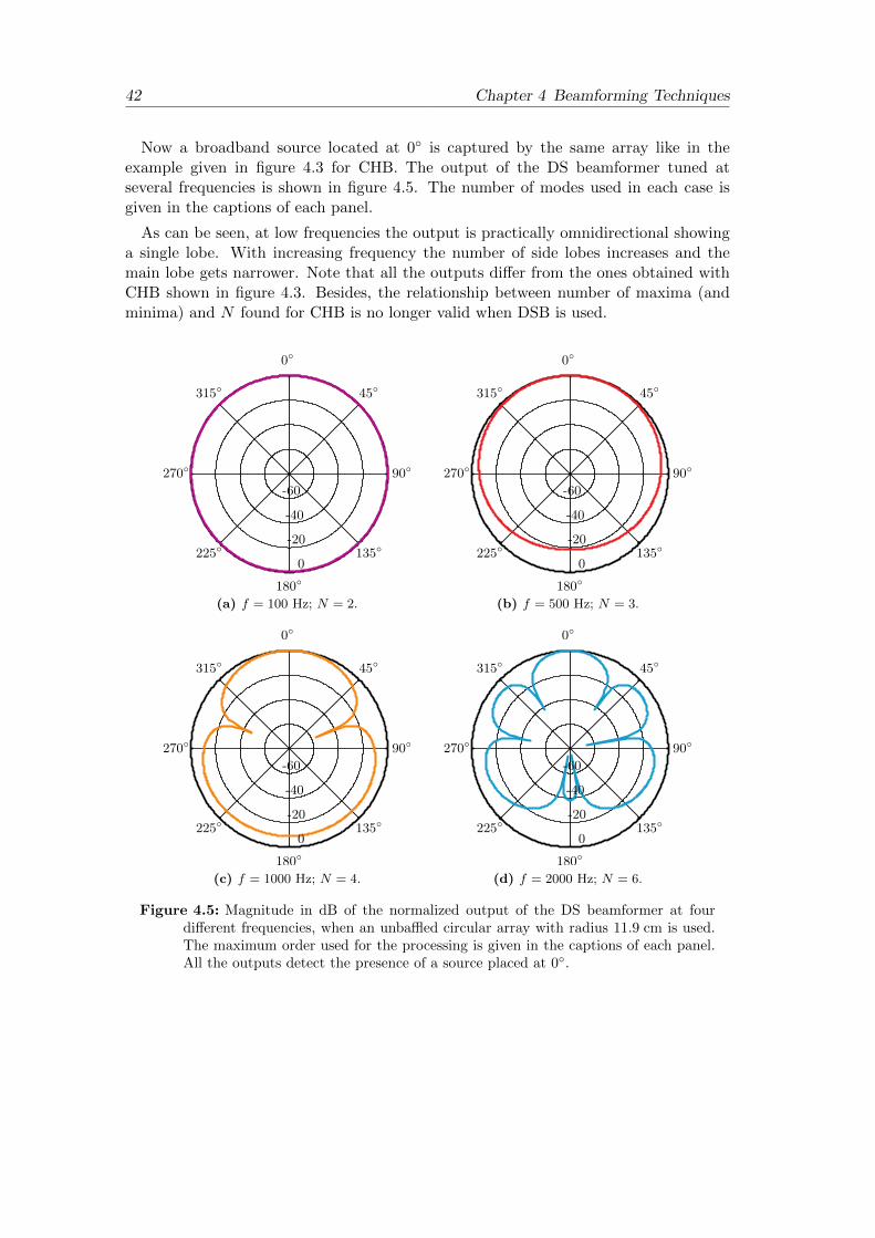
42 Chapter 4 Beamforming Techniques
Now a broadband source located at 0∘ is captured by the same array like in theexample given in figure 4.3 for CHB. The output of the DS beamformer tuned atseveral frequencies is shown in figure 4.5. The number of modes used in each case isgiven in the captions of each panel.
As can be seen, at low frequencies the output is practically omnidirectional showinga single lobe. With increasing frequency the number of side lobes increases and themain lobe gets narrower. Note that all the outputs differ from the ones obtained withCHB shown in figure 4.3. Besides, the relationship between number of maxima (andminima) and N found for CHB is no longer valid when DSB is used.
0∘
45∘
90∘
135∘
180∘
225∘
270∘
315∘
-60
-40
-20
0
(a) f = 100 Hz; N = 2.
0∘
45∘
90∘
135∘
180∘
225∘
270∘
315∘
-60
-40
-20
0
(b) f = 500 Hz; N = 3.
0∘
45∘
90∘
135∘
180∘
225∘
270∘
315∘
-60
-40
-20
0
(c) f = 1000 Hz; N = 4.
0∘
45∘
90∘
135∘
180∘
225∘
270∘
315∘
-60
-40
-20
0
(d) f = 2000 Hz; N = 6.
Figure 4.5: Magnitude in dB of the normalized output of the DS beamformer at fourdifferent frequencies, when an unbaffled circular array with radius 11.9 cm is used.The maximum order used for the processing is given in the captions of each panel.All the outputs detect the presence of a source placed at 0∘.

4.5 Beamformer Performance 43
4.5 Beamformer Performance
Throughout the examples given for CHB and DSB it has been seen that the patternof the output of a beamformer varies from one technique to the other and also variesjust by changing the frequency. For these reasons, it is necessary to evaluate theperformance of a beamformer. This is done by means of the following measures: theresolution and the maximum side lobe level (MSL).
4.5.1 Resolution
The resolution of a beamformer is defined as the −3 dB width of the main lobe ofthe beampattern [20]. In figure 4.6, the resolution is calculated from the output of abeamformer that captures the sound from a source placed at 's1 = 150∘. As expected,
RES
'L 'H
' [∘]
∣ ∣
b∣ ∣
2[dB]
0 30 60 90 120 150 180 210 240 270 300 330 360−35
−30
−25
−20
−15
−10
−5
0
5
Figure 4.6: Calculation of the resolution for a given beamformer output.
the beampattern presents a main lobe with a maximum in the direction of the source's1. In the main lobe, there are two angles 'L and 'H at which the magnitude withrespect to the position of the maximum has decreased by −3 dB. These two anglesdetermine the resolution as follows
RES = 'H − 'L. (4.28)
This parameter is of interest because it gives an approximation to the minimum an-gular difference between two incoherent sources that is necessary in order for them tobe distinguished. In other words, if the angular difference between the sources is equalor exceeds the resolution, the beampattern presents two maxima that correspond tothe source positions, and hence they can be resolved. Panel (a) in figure 4.7 shows thebeampattern that is measured when two incoherent sources with the same characteris-

44 Chapter 4 Beamforming Techniques
tics are active. One of the sources is placed at 's1 = 150∘, like in the above example,whereas the second one is placed at 's2 = 's1 +RES.
' [∘]
∣ ∣
b∣ ∣
S1S2S1+S2
RES
0 30 60 90 120 150 180 210 240 270 300 330 3600
0.2
0.4
0.6
0.8
1
(a) Δs = RES.
' [∘]
∣ ∣
b∣ ∣
S1S2S1+S2
RES
0 30 60 90 120 150 180 210 240 270 300 330 3600
0.2
0.4
0.6
0.8
1
(b) Δs < RES.
Figure 4.7: Normalized beamformer output measured when two incoherent sources(S1+S2) are active. In the top panel, the sources are away from each other withan angular distance (Δs) that equals the resolution, whereas in the bottom panelthe angular distance is smaller than the resolution. The normalized beamformeroutputs are also shown for the sources being active separately.

4.5 Beamformer Performance 45
In such situation, it can be seen that the beamformer output reveals two maximathat coincide with the maxima that would be obtained with each source being activeindependently. On the contrary, when the angular difference between the sources issmaller than the resolution they cannot be resolved. This is shown in panel (b) infigure 4.7. As can be seen, the beamformer output gives a single maximum locatedin between the angles of the sources, and therefore, just one ‘non-existent’ source isidentified instead of the two actual sources.
A Matlab function that calculates the resolution for a given beamformer output canbe found in appendix B.3.1.
4.5.2 Maximum Side Lobe Level
As mentioned previously, the beamformer output usually presents side lobes aroundthe main lobe. This is an unwanted effect as the beamformer seems to be sensitivenot only in the focusing direction, i. e. the direction of the ‘real source’, but also in thedirection of ‘ghost sources’. For this reason, it is useful to evaluate the beamformerresponse by means of the MSL. This parameter is given by the difference between thepeak of the main lobe and the peak of the highest side lobe [21]. The calculation of theMSL is illustrated in figure 4.8.
In appendix B.3.2, the source code implemented for the calculation of the MSL canbe seen.
MSL
' [∘]
∣b∣2
[dB]
0 30 60 90 120 150 180 210 240 270 300 330 360−35
−30
−25
−20
−15
−10
−5
0
5
Figure 4.8: Calculation of the MSL for a given beamformer output.


5Array Design and Simulations
5.1 Introduction
The design of any array is mainly determined by the purpose of the array and thesignal processing techniques that are used. In our case, the aim of the array is thelocalization of environmental noise sources, e. g. motorways, trains, etc. This meansthat the array is placed outdoors, under free-field conditions. In such case, we assumethat the array captures the sound field created by sources placed in the far-field. Thismakes it possible to consider that the waves that impinge on the array are planarand that they propagate in parallel to the ground, perpendicularly to the z-axis, i. e.reflections from the sky are inexistent and reflections from the ground are sufficientlyattenuated. This requirement is fulfilled by circular arrays since they can be deployedin situations where the sound field is two-dimensional. In the actual case, the arrayshould be placed in parallel to the ground to capture the sound field in the xy-plane, asdepicted in figure 5.1. Besides, all the directions in this plane have the same importance,which implies that the array microphones must be omnidirectional.
sourceki
x
yz
Figure 5.1: Layout of a circular array used to localize environmental noise sources. Thewaves that impinge on the array are planar and their direction of propagation isparallel to ground.
47

48 Chapter 5 Array Design and Simulations
Concerning environmental noise, the frequency range under consideration is oftenbroadband. The problem is that the frequency range of arrays is limited. Therefore,the array should be sensitive at those frequencies where the presence of noise is moresevere. In this sense, the frequency range of the array is chosen in section 5.2, wherethe spectral behavior of some sources of interest is presented.
There are two main requirements in the design of the array:
� It must be relatively small and portable, since it is meant to be used in outdoormeasurements. According to this, the maximum radius of the array that is takeninto account is 20 cm.
� The number of microphones must be moderate in order to lower expenses.
In terms of signal processing it is convenient to use beamforming techniques as theyare suitable for far-field measurements. The techniques that will be analyzed are CHBand DSB. As mentioned in chapters 3 and 4, several parameters play a role when dealingwith CHB and DSB, namely the radius of the array, the number of microphones, thenumber of modes used to decompose the sound field or the dynamic range in termsof kR. Therefore, it becomes necessary to make use of simulations and base the finaldesign of the array on their results.
5.2 Environmental Noise Sources
The frequency content of the noise created by several environmental sources has beenmeasured with a Bruel & Kjær Hand-held sound level meter B&K Type 2250. A shortdescription of the measured sources and the measurement procedure is given in thefollowing:
� Motorway. The sound from the motorway from Helsingør to Copenhagen hasbeen measured in the surroundings of Kgs. Lyngby at about 4 m away from themotorway. Ten measurements of one minute each have been performed.
� Airports. The sound from several airplanes taking off has been measured inDragør in front of one of the main lanes of Copenhagen Airport. The distance tothe airplanes is about 40 m in the moment of the taking off. Each measurementhas been started when the airplane started to accelerate before the taking offand has been stopped when the sound is no longer perceived at the measurementpoint.
� Trains. The sound produced by S-tog trains when they arrive or leave LyngbyStation has been measured at a distance of 50 cm away from the railway at thestation. In the case of trains arriving, the measurements start when the sound isperceived for the first time and stop after the trains stop in the station. For trainsleaving the station, the measurements start after the trains doors are closed andthey are stopped when the sound totally vanishes.
Besides, the sound of trains passing by has been also measured in the surroundingsof Lyngby Sø, in Kgs. Lyngby. The measurement position is about 2 m away fromthe railway. The measurements start when the sound of trains is heard for thefirst time and stop when the sound vanishes.

5.2 Environmental Noise Sources 49
All the measurements of equivalent sound pressure level performed in each situationhave been averaged. Figures 5.2 to 5.4 show the averaged equivalent sound pressurelevel of each kind of source, with and without A-weighting.
Frequency [Hz]
Lev
el[d
B]
Leq
LAeq
100 1k 10k-10
0
10
20
30
40
50
60
70
Figure 5.2: Equivalent sound pressure of airplanes taking off. This is the result of aver-aging 10 measurements of 10 min each.
Frequency [Hz]
Lev
el[d
B]
Leq
LAeq
100 1k 10k-20
-10
0
10
20
30
40
50
60
Figure 5.3: Equivalent sound pressure of a motorway. This is the result of averaging 10measurements of 10 min each.
In the case of train, the spectrum in all three situations (passing by, arriving andleaving the station) presents frequency content in the same frequency range. For this
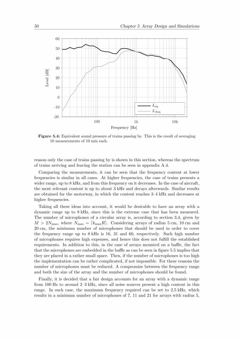
50 Chapter 5 Array Design and Simulations
Frequency [Hz]
Lev
el[d
B]
Leq
LAeq
100 1k 10k-20
-10
0
10
20
30
40
50
60
Figure 5.4: Equivalent sound pressure of trains passing by. This is the result of averaging10 measurements of 10 min each.
reason only the case of trains passing by is shown in this section, whereas the spectrumof trains arriving and leaving the station can be seen in appendix A.4.
Comparing the measurements, it can be seen that the frequency content at lowerfrequencies is similar in all cases. At higher frequencies, the case of trains presents awider range, up to 8 kHz, and from this frequency on it decreases. In the case of aircraft,the most relevant content is up to about 3 kHz and decays afterwards. Similar resultsare obtained for the motorway, in which the content reaches 3–4 kHz and decreases athigher frequencies.
Taking all these ideas into account, it would be desirable to have an array with adynamic range up to 8 kHz, since this is the extreme case that has been measured.The number of microphones of a circular array is, according to section 3.4, given byM > 2Nmax, where Nmax = ⌈kmaxR⌉. Considering arrays of radius 5 cm, 10 cm and20 cm, the minimum number of microphones that should be used in order to coverthe frequency range up to 8 kHz is 16, 31 and 60, respectively. Such high numberof microphones requires high expenses, and hence this does not fulfill the establishedrequirements. In addition to this, in the case of arrays mounted on a baffle, the factthat the microphones are embedded in the baffle as can be seen in figure 5.5 implies thatthey are placed in a rather small space. Then, if the number of microphones is too highthe implementation can be rather complicated, if not impossible. For these reasons thenumber of microphones must be reduced. A compromise between the frequency rangeand both the size of the array and the number of microphones should be found.
Finally, it is decided that a fair design accounts for an array with a dynamic rangefrom 100 Hz to around 2–3 kHz, since all noise sources present a high content in thisrange. In such case, the maximum frequency required can be set to 2.5 kHz, whichresults in a minimum number of microphones of 7, 11 and 21 for arrays with radius 5,
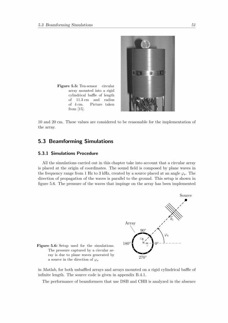
5.3 Beamforming Simulations 51
Figure 5.5: Ten-sensor circulararray mounted into a rigidcylindrical baffle of lengthof 11.3 cm and radiusof 4 cm. Picture takenfrom [15].
10 and 20 cm. These values are considered to be reasonable for the implementation ofthe array.
5.3 Beamforming Simulations
5.3.1 Simulations Procedure
All the simulations carried out in this chapter take into account that a circular arrayis placed at the origin of coordinates. The sound field is composed by plane waves inthe frequency range from 1 Hz to 3 kHz, created by a source placed at an angle 's. Thedirection of propagation of the waves is parallel to the ground. This setup is shown infigure 5.6. The pressure of the waves that impinge on the array has been implemented
Figure 5.6: Setup used for the simulations.The pressure captured by a circular ar-ray is due to plane waves generated bya source in the direction of 's.
x
y
0∘
90∘
270∘
180∘
Source
's
kiArray
in Matlab, for both unbaffled arrays and arrays mounted on a rigid cylindrical baffle ofinfinite length. The source code is given in appendix B.4.1.
The performance of beamformers that use DSB and CHB is analyzed in the absence

52 Chapter 5 Array Design and Simulations
of noise, i. e. in ideal conditions, as a first approach. Afterwards, the influence ofbackground noise is investigated. The response of the beamformers is calculated inthe frequency range of interest, with a resolution of 1 Hz. Besides, the beamformersresponse is obtained for all the angles ' from 0 to 2� rad, with an angular resolutionof 0.005 rad (or 0.286∘).
The arrays under test are unbaffled and mounted on a rigid cylindrical baffle of infinitelength. According to the previous sections, the radius of the arrays must be 20 cm atmost and their dynamic range should be from 100 Hz up to 2–3 kHz. Following theserequirements, arrays of radius 5, 10 and 20 cm are used for the simulations. The highestfrequency is set to be at least 2.5 kHz. Inserting this frequency into the relationshipN = ⌈kR⌉ by means of the wavenumber k (k = 2�f/c), the maximum order neededfor the beamforming algorithms (see equations (4.20) and (4.25)) follows
Nmax =
⌈2�freqc
R
⌉. (5.1)
As the number of microphones must fulfill M > 2Nmax, the minimum number ofmicrophones needed for each array is M = 2Nmax +1. When the condition M > 2Nmax
is not respected, a sampling error arises. An approximation of the maximum frequencythat can be used without having severe error due to sampling is determined by meansof the higher value kR
Nmax = kmaxR ⇒ fmax =Nmaxc
2�R.
Table 5.1 states the characteristics of the arrays used in the simulations that follow fromthe previous relationships, in terms of radius, maximum number of orders, number ofmicrophones and maximum frequency allowed to avoid sampling error.
Table 5.1: Features of the arrays used in the simulations. Note that the number of mi-crophones is the minimum required.
R [cm] Nmax M fmax [Hz]
Array 1 5 3 7 3275Array 2 10 5 11 2729Array 3 20 10 21 2729
5.3.2 Circular Harmonics Beamforming
5.3.2.1 Performance in Ideal Conditions
In this section, the results of several simulations carried out without the influenceof background noise are shown. In order to compare the beamforming techniques andthe cases of baffled and unbaffled arrays, a source placed at 180∘ has been used inall the simulations. In all cases, the displayed frequency range is up to 3 kHz whichcorresponds to the frequency content of the source. It is assumed that the amplitudeof the waves is the same for all frequencies.

5.3 Beamforming Simulations 53
The directivity patterns obtained with CHB when the arrays of table 5.1 are unbaffledare shown in figure 5.7. As can be seen, all the responses present a main lobe in thedirection of the source at 180∘. The patterns of the three arrays are similar as inall cases they remain constant for a certain interval and then change. Besides, theseintervals are compressed when the radius increases. It turns out that this behavior iscaused by the ceiling function in the calculation of N , i. e. in N = ⌈kR⌉. For example,in the case of an array of 5 cm, the pattern is constant up to 1091 Hz as N = 1 inthis interval, and varies when N changes to 2, and varies a third time when N = 3.Accordingly, the total number of intervals where the pattern is constant is given by thevalue Nmax, which is stated in table 5.1 for each array under analysis. In addition tothis, the main lobe gets narrower and the number of side lobes raises progressively withincreasing N . As the array of 20 cm of radius presents the highest value of Nmax, itsresponse is the most directive.
Certain frequencies present an ‘unexpected’ response, as can be seen around 2.6 kHzfor the array of radius of 5 cm in panel (a) or around 2.1 kHz and 2.8 kHz for thearray of 10 cm, in panel (b). This phenomenon is due to the fact that the Fouriercoefficients obtained with unbaffled arrays present some dips at certain values kR (seesection 3.2.1). For example, in the case of the array of 5 cm, the problem occurs at2.6 kHz which leads to a spatial frequency of kR ≈ 2.4. According to figure 3.3 onpage 18, this value corresponds to the first dip of C∘0 . Those frequencies where thisphenomenon occurs cannot be resolved with precision. This effect is avoided when thearrays are mounted on a rigid cylindrical baffle of infinite length. The overall behaviorof the beamformers output when baffled arrays are used is qualitatively identical to theunbaffled case but without the problem of unresolved frequencies. This can be seen inappendix A.2.1.
As mentioned in the previous section, the arrays can be used up to a maximumfrequency fmax without having the influence of the error due to sampling. In thecases of the arrays of radius of 10 and 20 cm this value is around 2.7 kHz. Fromthis frequency on, the effect of the sampling error can be seen in the beampatternsthrough the magnitude of the side lobes which are higher than in the previous intervalof frequencies.
All these ideas are reflected in the resolution and the MSL. These parameters areshown for unbaffled arrays, using a logarithmic scale from 50 Hz to 3 kHz, in figure 5.8.
As can be seen, the resolution and the MSL are constant for a certain interval.For each array, these intervals correspond to the ones observed in the beamformerspatterns. The fact that the main lobe gets narrower from interval to interval resultsin the improvement of the resolution that can be observed. More intervals result ina better resolution, which is the case of the array of largest radius. The MSL followsthe same behavior than the resolution, improving when the number of orders is raised.The staircase pattern in the resolution and the MSL is also obtained with sphericalharmonics beamforming [20].
Both measures get worse in those frequencies that coincide with the dips in the Fouriercoefficients. Besides, at those frequencies that exceed fmax, the MSL is dramaticallyaffected by the sampling error. In contrast to this, the resolution keeps constant anunaltered at the very same frequencies.
The resolution and the MSL obtained with baffled arrays is shown in figures A.3 and
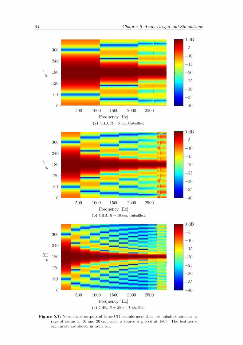
54 Chapter 5 Array Design and Simulations
(a) CHB, R = 5 cm, Unbaffled.
(b) CHB, R = 10 cm, Unbaffled.
(c) CHB, R = 20 cm, Unbaffled.
Figure 5.7: Normalized outputs of three CH beamformers that use unbaffled circular ar-rays of radius 5, 10 and 20 cm, when a source is placed at 180∘. The features ofeach array are shown in table 5.1.

5.3 Beamforming Simulations 55
A.4 in appendix A.2.1. These parameters are identical to the ones of the unbaffledarrays, but with the problem of the singularities at high frequencies solved.
Frequency [Hz]
RESCH[∘]
R = 5 cmR = 10 cmR = 20 cm
100 10000
20
40
60
80
100
120
(a)
Frequency [Hz]
MSLCH[dB]
R = 5 cmR = 10 cmR = 20 cm
100 1000−14
−13
−12
−11
−10
−9
−8
−7
(b)
Figure 5.8: Resolution and MSL of three CH beamformers that use unbaffled circulararrays of radius 5, 10 and 20 cm, when a source is placed at 180∘. The features ofeach array are given in table 5.1.
In order to analyze the dependency of resolution and MSL on the position of thesource, some simulations have been carried out for several frequencies as a function ofthe angle of the source 's. The resolution chosen for 's is 0.005 rad. The results are

56 Chapter 5 Array Design and Simulations
shown in figure 5.9 for the unbaffled array of 10 cm of radius. The frequencies used are100 Hz, 700 Hz, 1.2 kHz, 2 kHz and 2.5 kHz. For each frequency, the number of ordersneeded for the beamforming processing is different, which implies that the resolutionand the MSL are different in each case.
's [∘]
RESCH[∘]
f = 100 Hz
f = 700 Hz
f = 1.2 kHz
f = 2 kHz
f = 2.5 kHz
0 60 120 180 240 300 36020
40
60
80
100
120
(a)
's [∘]
MSLCH[dB]
f = 100 Hzf = 700 Hzf = 1.2 kHzf = 2 kHzf = 2.5 kHz
0 60 120 180 240 300 360−13
−12.5
−12
−11.5
−11
−10.5
−10
−9.5
(b)
Figure 5.9: Resolution and MSL as a function of the angular position of the source ob-tained with CHB and an unbaffled array of radius 10 cm at five different frequencies.The features of the array are given in table 5.1.

5.3 Beamforming Simulations 57
As can be seen, for each frequency the resolution is constant for all values of 's. TheMSL results are also constant except for the case of 2.5 kHz. This effect can be causedby the sampling error that starts to arise around fmax = 2.7 kHz. In the case of abaffled array with the same radius, which can be seen in appendix A.2.1, the resolutionslightly varies with 's at 2 kHz and 2.5 kHz, and the MSL presents more variation atthese precise frequencies.
The number of side lobes, shown in figure 5.10, has also been obtained for the sameunbaffled array as a function of source position. Like in the case of the MSL, the number
's [∘]
Number
ofSideLob
es
f = 100 Hzf = 700 Hzf = 1.2 kHzf = 2 kHzf = 2.5 kHz
0 60 120 180 240 300 3600
2
4
6
8
10
Figure 5.10: Number of side lobes as a function of the angular position of the sourceobtained with CHB and an unbaffled array of radius 10 cm at five different fre-quencies. The features of the array are given in table 5.1.
of side lobes is independent of 's except for the case of 2.5 Hz. At those frequencieswhere the number of side lobes is independent of 's, the number of side lobes follows
Number of Side Lobes = 2N − 1. (5.2)
For example, at 100 Hz, N = 1 and the pattern presents one side lobe; at 700 Hz,N = 2 and the number of side lobes is 3, etc. This behavior is also observed for baffledarrays (see figure A.5 in appendix A.2.1).
Even though it is not shown here, the same behavior is observed with arrays ofdifferent radius. From these results, one can say that the resolution, the MSL andthe number of side lobes obtained with CHB are independent of the source position inalmost all the frequency range of interest.
5.3.2.2 Performance with Influence of Background Noise
In order to analyze the beamformers performance in a more realistic situation, back-ground noise is introduced. The pressure captured by each microphone is then con-

58 Chapter 5 Array Design and Simulations
taminated with additive noise. The Signal-to-Noise ratio (SNR) in each microphone ofthe array is the ratio of the power of the signal without being contaminated with noiseover the power of the noise. It is considered that the spectral components of the noisecaptured by the microphones have the same magnitude. On the contrary, the noisephase, which is uniformly distributed from 0 to 2� rad, varies from one microphone tothe other. Therefore, the noise signals in the various microphones are uncorrelated.Then, at a given frequency, the SNR at each microphone follows
SNRm(f) =Psignal(f)
Pnoise(f)=∣Asignal∣2
∣Anoise∣2, (5.3)
where ∣Asignal∣ and ∣Anoise∣ are the magnitudes of the spectral components of the signaland the noise for a certain frequency. Note that they are independent of the frequencyas they have been assumed to be constant. For the simulations, an SNRm = 30 dB hasbeen used. A function that generates background noise for a required SNR has beenimplemented for the simulations and is provided in appendix B.4.2.
The simulations performed in ideal conditions are now repeated but inserting back-ground noise. A broadband source placed at 180∘ is again used. In figures 5.11 and5.12, the resolution and MSL obtained with unbaffled arrays are shown. At first
Frequency [Hz]
RESCH[∘]
R = 5 cmR = 10 cmR = 20 cm
100 10000
60
120
180
240
300
360
Figure 5.11: Resolution of three CH beamformers that use unbaffled circular arrays ofradius 5, 10 and 20 cm, when a source is placed at 180∘ and the SNR in the arraymicrophones is 30 dB. The features of each array are given in table 5.1.
glance, it can be seen that the resolution resembles the ideal case, with the differencethat instead of having continuous values in each interval, the responses present smallfluctuations caused by the presence of noise. At low frequencies, the amplitude of thesefluctuations is higher than in high frequencies. Besides, the response is poorer for thearray with the shortest radius.
The results obtained for MSL reveal that this measure is more sensitive to noise
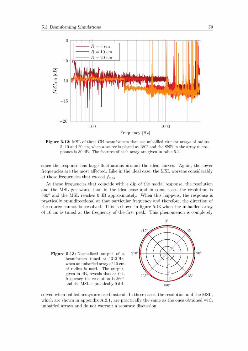
5.3 Beamforming Simulations 59
Frequency [Hz]
MSLCH[dB]R
R = 5 cmR = 10 cmR = 20 cm
100 1000−20
−15
−10
−5
0
Figure 5.12: MSL of three CH beamformers that use unbaffled circular arrays of radius5, 10 and 20 cm, when a source is placed at 180∘ and the SNR in the array micro-phones is 30 dB. The features of each array are given in table 5.1.
since the response has large fluctuations around the ideal curves. Again, the lowerfrequencies are the most affected. Like in the ideal case, the MSL worsens considerablyat those frequencies that exceed fmax.
At those frequencies that coincide with a dip of the modal response, the resolutionand the MSL get worse than in the ideal case and in some cases the resolution is360∘ and the MSL reaches 0 dB approximately. When this happens, the response ispractically omnidirectional at that particular frequency and therefore, the direction ofthe source cannot be resolved. This is shown in figure 5.13 when the unbaffled arrayof 10 cm is tuned at the frequency of the first peak. This phenomenon is completely
Figure 5.13: Normalized output of abeamformer tuned at 1313 Hz,when an unbaffled array of 10 cmof radius is used. The output,given in dB, reveals that at thisfrequency the resolution is 360∘
and the MSL is practically 0 dB.
0∘
45∘
90∘
135∘
180∘
225∘
270∘
315∘
-3
-2
-1
0
solved when baffled arrays are used instead. In these cases, the resolution and the MSL,which are shown in appendix A.2.1, are practically the same as the ones obtained withunbaffled arrays and do not warrant a separate discussion.

60 Chapter 5 Array Design and Simulations
The influence of noise can be analyzed by means of the CH beamformer response.When background noise contaminates the measurement, the pressure in each micro-phone is the summation of the pressure due to the source and the pressure of thenoise
ptotal(kR, 'm) = p(kR, 'm) + n(kR, 'm). (5.4)
Then, according to equation (4.19) on page 37, the output of the beamformer is
bN,CH(kR, ') = AN∑
n=−N
Cn(kR, 's)
Cn(kR, ')+
NnCn(kR, ')
, (5.5)
where Nn are the coefficients obtained by decomposing the noise in CH with the arrayusing equation (4.6) on page 34
Nn =1
M
M∑m=1
n(kR, 'm)e−jn'm . (5.6)
Let us suppose that the beamformer is steered to 's, so the first term in equation (5.5)approximates unity for all orders n as the theoretical and the approximated coefficientsbecome very similar. However, the coefficients of the noise do not have anything incommon with Cn. This can be seen in figure 5.14 where the coefficients of the noiseand the term 1/Cn are shown for orders up to 3 when an unbaffled array of 10 cm and11 microphones is used. The negative orders of 1/Cn are not given because they areexactly the same as the positive ones.
The noise coefficients Nn are just random noise uniformly distributed, whereas theterms 1/Cn do vary with order and kR. As can be seen, the zeroth order is constantat low values of kR. By contrast, higher orders present higher magnitudes which de-cay with increasing kR. With increasing order, the decay becomes faster. At highvalues kR, all orders present similar and rather small amplitudes, with the exceptionof some peaks that correspond to those frequencies that cannot be resolved. As men-tioned before, these can be removed by mounting the array on a baffle. Accordingto equation (5.5) the noise coefficients multiply the terms 1/Cn. As can be seen fromfigure 5.14, at low values kR, or equivalently at low frequencies, the noise coefficients oforder different from 0 are amplified. Then the noise gain more strength than the signaland this contaminates the beamformer processing. This explains why the resolutionand mostly the MSL are more influenced by noise at low frequencies. Besides this,there are other ideas concerning noise that must be analyzed in the following:
� The curves obtained for 1/Cn are independent of the array size. However, fora given frequency range, arrays with short radius present lower values kR incomparison with larger arrays. Taking into account that at lower values of kR thenoise is more amplified, it becomes obvious that smaller arrays are more affectedby noise. Because of this, the array with smallest radius is more influenced thanthe other arrays as observed in figures 5.11 and 5.12.
� According to the previous item, the terms 1/Cn are of greater amplitude withincreasing order, at low frequencies. Then, if the calculation of the beamformeroutput is done with more orders than necessary, the noise becomes more amplified.It has been seen that using N = ⌈kR⌉ the results in terms of MSL and resolution

5.3 Beamforming Simulations 61
kR
Magnitudeof
Nn[dB]
n = 0n = 1n = 2n = 3
0.1 1−80
−70
−60
−50
−40
−30
(a)
kR
Magnitudeof
1/Cn[dB]
n = 0n = 1n = 2n = 3
0.1 10
20
40
60
80
100
(b)
Figure 5.14: Top panel shows the magnitude of the first four coefficients obtained bydecomposing uniformly distributed noise with an unbaffled array of radius of 10 cmand 11 microphones. The noise is designed in order to have 30 dB of SNR at theinput of each microphone of the array. The power of the signal of the source in theinput of each microphone is −3 dB and the power of the noise is −33 dB. In thebottom panel, the magnitude of the inverse value of the coefficients Cn are depictedfor the first four coefficients. The features of the array are given in table 5.1.
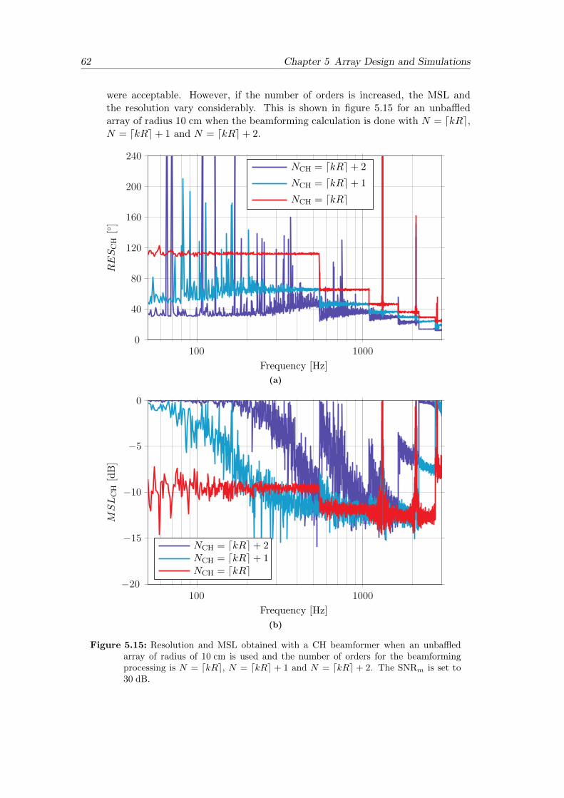
62 Chapter 5 Array Design and Simulations
were acceptable. However, if the number of orders is increased, the MSL andthe resolution vary considerably. This is shown in figure 5.15 for an unbaffledarray of radius 10 cm when the beamforming calculation is done with N = ⌈kR⌉,N = ⌈kR⌉+ 1 and N = ⌈kR⌉+ 2.
Frequency [Hz]
RESCH[∘]
NCH = ⌈kR⌉+ 2
NCH = ⌈kR⌉+ 1
NCH = ⌈kR⌉
100 10000
40
80
120
160
200
240
(a)
Frequency [Hz]
MSLCH[dB]CH
NCH = ⌈kR⌉+ 2NCH = ⌈kR⌉+ 1NCH = ⌈kR⌉
100 1000−20
−15
−10
−5
0
(b)
Figure 5.15: Resolution and MSL obtained with a CH beamformer when an unbaffledarray of radius of 10 cm is used and the number of orders for the beamformingprocessing is N = ⌈kR⌉, N = ⌈kR⌉ + 1 and N = ⌈kR⌉ + 2. The SNRm is set to30 dB.

5.3 Beamforming Simulations 63
It can be seen that at low frequencies the resolution and the MSL are more influ-enced by noise. In addition to this, the influence is stronger when the number ofused orders increases. At high frequencies the resolution improves with increasingthe number of orders, but at the same time the range where this occurs becomessmaller as the response is polluted with background noise in a wider frequencyrange. However, the MSL becomes worse in all frequency range when the numberof orders increases. Just when N = ⌈kR⌉+ 1 the MSL is better or similar to thecase of N = ⌈kR⌉ in the range from 300 Hz to 2 kHz. In conclusion, if the array isrequired to cover a wide frequency range, the best option is to choose N = ⌈kR⌉.
The last feature that is investigated is the influence of the number of microphones inthe array. This is exemplified in figures 5.16 and 5.17 for an unbaffled array of 10 cm ofradius when the number of microphones is the minimum required plus one more. Thereason for choosing only these two different number of microphones is that with thesenumbers, 11 and 12, the relationship between M and N , i. e. M > 2N , admits the samemaximum order N in both cases. In other words, as stated in table 5.1 on page 52,the maximum number of orders that can be used with an array of radius 10 cm and 11microphones is 5. With 12 microphones, the maximum number of orders is still 5. Ifthe number of microphones is increased to 13, the maximum number of orders is then 6,which implies that the response improves towards the higher frequencies with respect tothose cases where the maximum number of orders is 5. Therefore, in order to comparethe responses in the same conditions in terms of maximum order (and frequency range),the number of microphones can only be 11 or 12.
Frequency [Hz]
RESCH[∘]
M = 11M = 12
100 10000
40
80
120
160
200
Figure 5.16: Resolution obtained with a CH beamformer when an unbaffled array ofradius of 10 cm is used with 11 and 12 microphones. The SNRm is set to 30 dB.
As can be seen, the result of using one more microphone than the minimum neces-sary do not have any significant influence in terms of resolution, but the MSL slightlyimproves at frequencies above fmax.

64 Chapter 5 Array Design and Simulations
Frequency [Hz]
MSLCH[dB]
M = 11M = 12
100 1000−16
−14
−12
−10
−8
−6
−4
−2
0
Figure 5.17: MSL obtained with a CH beamformer when an unbaffled array of radius of10 cm is used with 11 and 12 microphones. The SNRm is set to 30 dB.
5.3.3 Delay-and-Sum Beamforming
5.3.3.1 Performance in Ideal Conditions
The beampatterns obtained in ideal conditions by means of DSB are shown in fig-ure 5.18, when unbaffled arrays of radius 5, 10 and 20 cm are considered. Note thatagain, a broadband source placed at 180∘ has been used. In DSB, the number of ordersused for the processing is N = ⌈kR⌉+1. Later on, the reason for this will be explained.
As can be seen, the patterns are in all cases omnidirectional at low frequencies. Withincreasing frequency the main beam gets narrower and narrower and the number of sidelobes increases. In addition to this, the beampattern becomes more directive when theradius of the array is increased. Approximately below fmax, the side lobes gain strengthin all cases, meaning that the sampling error arises. However, this error is not as obviousas in CHB. Apart from this, there are other differences from CHB, for instance, the lowerfrequencies are totally omnidirectional, the output varies continuously with frequencyand all high frequencies can be resolved.
The patterns obtained with baffled arrays are shown in appendix A.2.2. In terms ofdirectivity they are similar to the unbaffled case. However, they present some differencesthat will be analyzed by means of the resolution and the MSL. These two measures areshown in figure 5.19 for both baffled and unbaffled arrays.
As can be seen in all cases, at low frequencies the resolution is 360∘ and the MSL isnon-existent, as the beamformers are omnidirectional. From a certain frequency thatdepends on the beamformer, the resolution improves continuously until high frequen-cies. The curves decay in a similar way for both kinds of arrays, but in the baffled casethey present very smooth fluctuations. The MSL curves begin in a certain frequencyand grow progressively until a maximum level. In the case of unbaffled arrays, this level

5.3 Beamforming Simulations 65
(a) DSB, R = 5 cm, Unbaffled.
(b) DSB, R = 10 cm, Unbaffled.
(c) DSB, R = 20 cm, Unbaffled.
Figure 5.18: Normalized outputs of three DS beamformers that use unbaffled circulararrays of radius 5, 10 and 20 cm, when a source is placed at 180∘. The features ofeach array are shown in table 5.1.

66 Chapter 5 Array Design and Simulations
Frequency [Hz]
RESDS[∘]
R = 5 cmR = 10 cmR = 20 cm
100 10000
60
120
180
240
300
360
(a)
Frequency [Hz]
MSLDS[dB]
R = 5 cmR = 10 cmR = 20 cm
100 1000−70
−60
−50
−40
−30
−20
−10
0
(b)
Figure 5.19: Resolution and MSL of three DS beamformers that use both baffled andunbaffled circular arrays of radius 5, 10 and 20 cm, when a source is placed at180∘. The responses of the unbaffled arrays are the ones with continuous lines,whereas the responses for the baffled arrays are dashed. The features of each arrayare given in table 5.1.

5.3 Beamforming Simulations 67
is kept constant, whereas for baffled arrays the MSL presents smooth ripples while itincreases towards high frequencies. Nevertheless, the MSL is better for baffled arraysthan for unbaffled.
Independently of baffled or unbaffled arrays, the performance improves with increas-ing the radius of the arrays and is better in the case of baffled arrays. Furthermore,it can be seen that the baffled array of 5 cm of radius has a resolution similar to theunbaffled array of radius 10 cm, the resolution of the baffled array of 10 cm is similarto the one of the unbaffled array of 20 cm, etc. Therefore, the fact of mounting thearray on an infinite baffle makes the array appear to be ‘larger’ than in the unbaffledcase. This tendency can also be observed in the MSL curves. Similar characteristicsare found when DSB is applied to spherical arrays [20].
In general, it can be said that the resolution obtained with DSB is much worse thanthe one obtained with CHB because in that case all the frequency range was ‘covered’,whereas with DSB only high frequencies are resolved with accuracy but low frequenciesare totally unresolved. At high frequencies, the MSL using DSB is worse than in CHBwhen unbaffled arrays are used. Despite of this, just the opposite occurs when dealingwith baffled arrays.
It is interesting to analyze if the resolution and the MSL are independent of theposition of the source. Like in the case of CHB, this is done for a specific frequency asa function of 's. The resolution and MSL obtained with an unbaffled array of 10 cm areshown in figures 5.20 and 5.21. The frequencies used previously with CHB in figures 5.9and 5.10 are chosen again. The resolution used for 's is 0.005 rad.
's [∘]
RESDS[∘]
f = 700 Hz
f = 1.2 kHz
f = 2 kHz
f = 2.5 kHz
0 60 120 180 240 300 3600
50
100
150
200
250
300
350
400
Figure 5.20: Resolution obtained using DSB with an unbaffled array of radius 10 cmat different frequencies as a function of the angular position of the source. Thefeatures of the array are given in table 5.1.
These results reveal that the resolution and the MSL are independent of the sourceposition at frequencies up to 2.5 kHz. In the case of a baffled array, which is shown

68 Chapter 5 Array Design and Simulations
's [∘]
MSLDS[dB]
f = 700 Hz
f = 1.2 kHz
f = 2 kHz
f = 2.5 kHz
0 60 120 180 240 300 360
−22
−20
−18
−16
−14
−12
−10
−8
Figure 5.21: MSL obtained using DSB with an unbaffled array of radius 10 cm at differentfrequencies as a function of the angular position of the source. The features of thearray are given in table 5.1.
in figure A.12 in appendix A.2.2, a dependency of the angle can be seen at 2 kHz and2.5 kHz.
5.3.3.2 Performance with Influence of Background Noise
The performance of DS beamformers must be evaluated in realistic situations thataccount for background noise. Like in the case of CHB, the SNR at the input of eacharray microphone (SNRm) is set to 30 dB.
The resolution and the MSL when background noise is present is given in figure 5.22when unbaffled arrays are used. As can be seen, the results of both resolution and MSLfollow the curves obtained for the ideal case rather accurately. This is also obtainedwith baffled arrays as can be seen in appendix A.2.2. In contrast with CHB, DSB ismore robust to background noise.
Similarly to CHB, the influence of noise on a DS beamformer can be deduced by in-serting the relationships found in equations (5.4) and (5.6) into the beamformer outputgiven in equation (4.26) on page 41. This is
bN (kR, ') =N∑
n=−NCn(kR, 's)C∗n(kR, ') +NnC∗n(kR, '). (5.7)
Assuming ' = 's, the first term in the summation is approximately ∣Cn(kR, 's)∣2 andthe second one is random noise that multiplies the coefficients shown in figures 3.3 onpage 18 or 3.5 on page 19, depending on the condition of baffled or unbaffled. Fororders higher than 0, these coefficients, which present a high-pass filter characteristic

5.3 Beamforming Simulations 69
Frequency [Hz]
RESDS[∘]
R = 5 cmR = 10 cmR = 20 cm
100 10000
60
120
180
240
300
360
(a)
Frequency [Hz]
MSLDS[dB]
R = 5 cmR = 10 cmR = 20 cm
100 1000−45
−40
−35
−30
−25
−20
−15
−10
−5
(b)
Figure 5.22: Resolution and MSL of three DS beamformers that use unbaffled circulararrays of radius 5, 10 and 20 cm, when a source is placed at 180∘ and the SNR inthe array microphones is 30 dB. The features of each array are given in table 5.1.

70 Chapter 5 Array Design and Simulations
with steeper roll-off as the order increases, attenuate the background noise. This makesthe response of the DS beamformer more influenced by the first term (the one thatcontains the information about the source) than by the noise term.
In contrast to CHB, it becomes obvious from the foregoing reasoning that whenthe maximum number of orders used for the DS beamformer is increased the noisecontribution is practically unaltered. For CHB it turns out that the best option for theprocessing is when N = ⌈kR⌉, but for DSB this is no longer necessary. In figures 5.23and 5.24, the resolution and the MSL for the cases N = ⌈kR⌉ and N = ⌈kR⌉ + 1are shown using a DS beamformer. An unbaffled array of 10 cm of radius has beenconsidered.
Frequency [Hz]
RESDS[∘]
⌈
NDS = ⌈kR⌉NDS = ⌈kR⌉+ 1
100 10000
60
120
180
240
300
360
Figure 5.23: Resolution obtained using DSB with an unbaffled array of radius 10 cmwhen the number of modes used for the beamforming processing is N = ⌈kR⌉ andN = ⌈kR⌉+ 1. The SNRm is set to 30 dB.
As can be seen, the results are very similar for both values of N , but slightly betterwhen N = ⌈kR⌉+ 1.
Even though it is not shown here, when the number of orders is further increased nosignificant improvement with respect to the case of N = ⌈kR⌉ + 1 results.1 For thisreason, N = ⌈kR⌉+ 1 is preferred for the DSB processing.2
Like in the case of CHB, the number of microphones has been increased in order toexamine the effect. However, no improvement has been detected. This is illustrated infigure A.13 in appendix A.2.2, where the performance of an unbaffled array of 10 cmwith 11 and 12 microphones is shown.
1A detailed mathematical proof can be found in appendix A.5.2Note that in all figures of this document that concern DSB, the number of orders have always followedN = ⌈kR⌉ + 1.
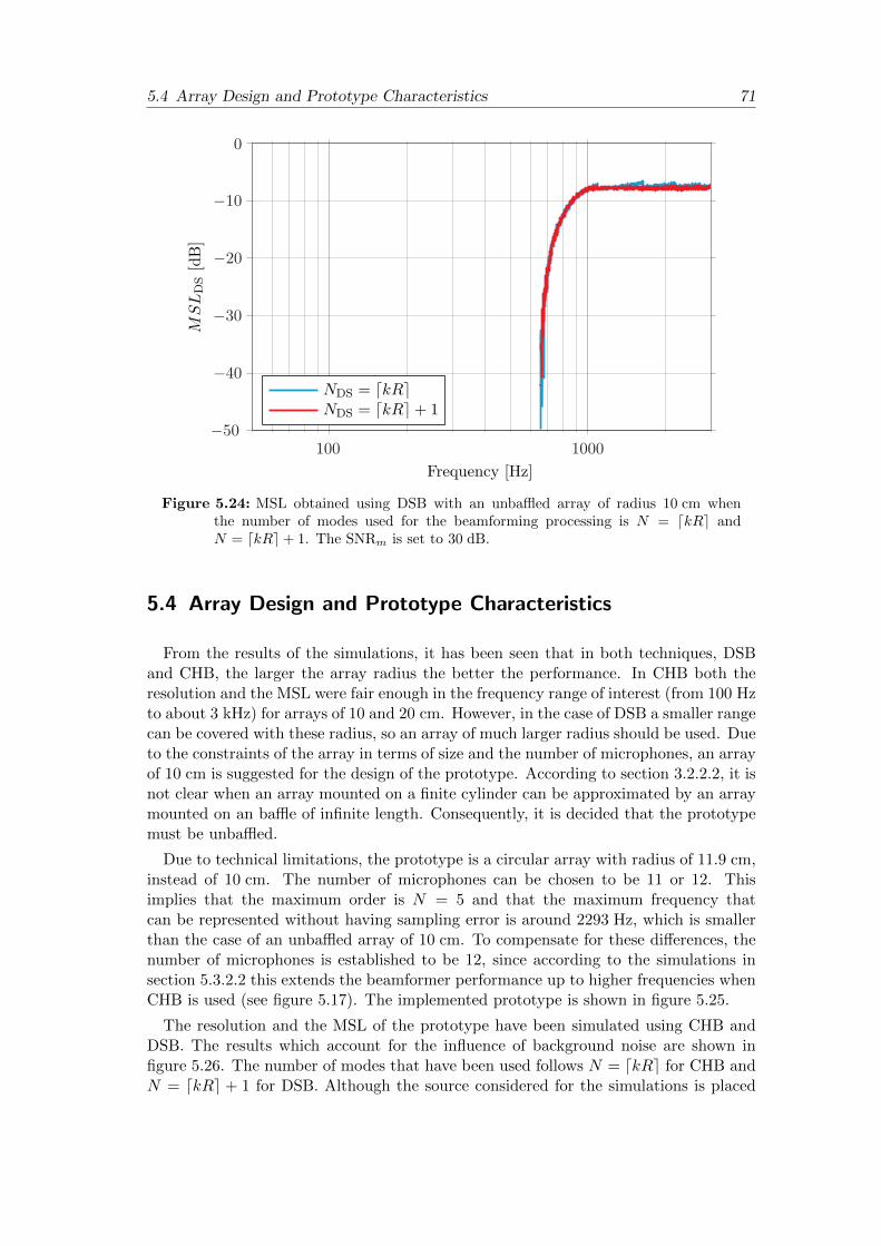
5.4 Array Design and Prototype Characteristics 71
Frequency [Hz]
MSLDS[dB]
⌈
NDS = ⌈kR⌉NDS = ⌈kR⌉+ 1
100 1000−50
−40
−30
−20
−10
0
Figure 5.24: MSL obtained using DSB with an unbaffled array of radius 10 cm whenthe number of modes used for the beamforming processing is N = ⌈kR⌉ andN = ⌈kR⌉+ 1. The SNRm is set to 30 dB.
5.4 Array Design and Prototype Characteristics
From the results of the simulations, it has been seen that in both techniques, DSBand CHB, the larger the array radius the better the performance. In CHB both theresolution and the MSL were fair enough in the frequency range of interest (from 100 Hzto about 3 kHz) for arrays of 10 and 20 cm. However, in the case of DSB a smaller rangecan be covered with these radius, so an array of much larger radius should be used. Dueto the constraints of the array in terms of size and the number of microphones, an arrayof 10 cm is suggested for the design of the prototype. According to section 3.2.2.2, it isnot clear when an array mounted on a finite cylinder can be approximated by an arraymounted on an baffle of infinite length. Consequently, it is decided that the prototypemust be unbaffled.
Due to technical limitations, the prototype is a circular array with radius of 11.9 cm,instead of 10 cm. The number of microphones can be chosen to be 11 or 12. Thisimplies that the maximum order is N = 5 and that the maximum frequency thatcan be represented without having sampling error is around 2293 Hz, which is smallerthan the case of an unbaffled array of 10 cm. To compensate for these differences, thenumber of microphones is established to be 12, since according to the simulations insection 5.3.2.2 this extends the beamformer performance up to higher frequencies whenCHB is used (see figure 5.17). The implemented prototype is shown in figure 5.25.
The resolution and the MSL of the prototype have been simulated using CHB andDSB. The results which account for the influence of background noise are shown infigure 5.26. The number of modes that have been used follows N = ⌈kR⌉ for CHB andN = ⌈kR⌉ + 1 for DSB. Although the source considered for the simulations is placed
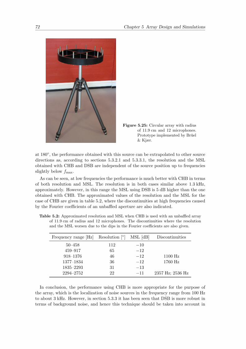
72 Chapter 5 Array Design and Simulations
Figure 5.25: Circular array with radiusof 11.9 cm and 12 microphones.Prototype implemented by Bruel& Kjær.
at 180∘, the performance obtained with this source can be extrapolated to other sourcedirections as, according to sections 5.3.2.1 and 5.3.3.1, the resolution and the MSLobtained with CHB and DSB are independent of the source position up to frequenciesslightly below fmax.
As can be seen, at low frequencies the performance is much better with CHB in termsof both resolution and MSL. The resolution is in both cases similar above 1.3 kHz,approximately. However, in this range the MSL using DSB is 5 dB higher than the oneobtained with CHB. The approximated values of the resolution and the MSL for thecase of CHB are given in table 5.2, where the discontinuities at high frequencies causedby the Fourier coefficients of an unbaffled aperture are also indicated.
Table 5.2: Approximated resolution and MSL when CHB is used with an unbaffled arrayof 11.9 cm of radius and 12 microphones. The discontinuities where the resolutionand the MSL worsen due to the dips in the Fourier coefficients are also given.
Frequency range [Hz] Resolution [∘] MSL [dB] Discontinuities
50–458 112 −10459–917 65 −12918–1376 46 −12 1100 Hz1377–1834 36 −12 1760 Hz1835–2293 31 −132294–2752 22 −11 2357 Hz; 2536 Hz
In conclusion, the performance using CHB is more appropriate for the purpose ofthe array, which is the localization of noise sources in the frequency range from 100 Hzto about 3 kHz. However, in section 5.3.3 it has been seen that DSB is more robust interms of background noise, and hence this technique should be taken into account in

5.4 Array Design and Prototype Characteristics 73
noisy environments. Furthermore, DSB can be used to resolve those high frequencieswhere CHB presents discontinuities.
Frequency [Hz]
RES
[∘]
CHBDSB
100 10000
60
120
180
240
300
360
(a)
Frequency [Hz]
MSL
[dB]
CHBDSB
100 1000−50
−40
−30
−20
−10
0
(b)
Figure 5.26: Simulated resolution and MSL of an unbaffled array of 11.9 cm of radiusand 12 microphones when CHB and DSB are used. A source at 180∘ has beenconsidered and the SNRm has been set to 30 dB.


6Measurement Results and
Discussion
6.1 Measurement Setup
A circular array of radius 11.9 cm with 12 equidistant microphones has been testedin an anechoic chamber at the Acoustic Technology Department of the Technical Uni-versity of Denmark (DTU).
The array is conformed by 1/4 ”microphones B&K Type 4935 embedded on a circularframe every 30∘. In all the measurements, it stands on a turntable B&K Type 5960.The turntable is placed on a support that is anchored to the ground of the room whichis about 3 m below the support. In figure 6.1, a sketch of the arrangement of theequipment in the anechoic chamber can be seen. The array position is kept along the
Figure 6.1: Arrangement of theequipment in the anechoicroom.
x
y support
array
wedges
11.8 m
9.2 m
75

76 Chapter 6 Measurement Results and Discussion
measurements at x = 4.5 m, y = 3.8 m and z = 4 m according to the coordinates givenin the sketch. The equipment setup used for the measurements is shown in figure 6.2.The characteristics of all the equipment are described in appendix C.
Amplifier
Computer
MicrophonesB&K 4935
PULSE Analyzer
12 input
Anechoic room
Turntable B&K 5960
Multichannel
outputGenerator
TurntableController
B&K 5960
channels
Source
Figure 6.2: Equipment setup. The array and the source are controlled by a PULSEAnalyzer and the turntable is managed by its own controller.
The array and the source are controlled by means of a Bruel & Kjær MultichannelPULSE Analyzer that includes various input-channels and one generator output. In allthe measurements, the signal from the generator feeds the source after being amplified.In order to excite the entire frequency range of the array in each measurement, thegenerator signal is pseudorandom noise of 1 s of period, 3.2 kHz of bandwidth and1 Hz of resolution. The advantage of using pseudorandom noise is that each frequencycomponent has the same amplitude in each period, and hence the average over severalperiods is not necessary.
The signals captured by the microphones of the array are recorded with the analyzer.Note that these signals are the result of the loudspeaker signal at the measurementpoint plus background noise. The signals are then processed with the beamformingalgorithms DSB and CHB developed in chapter 4. For the processing, an angularresolution of 0.005 rad is used, and the number of orders used to decompose the soundfield is N = ⌈kR⌉ for CHB and N = ⌈kR⌉+ 1 for DSB.
In all measurements, the source, which is a loudspeaker unit mounted on a sphere,hangs from the ceiling of the anechoic room in order to keep it as static as possible.This can be seen in figure 6.3. The source is placed far enough from the array so theimpinging waves are created in the far-field.
To evaluate the performance of the array for different angular directions of the source,the source is kept still at a certain position, whereas the array is moved around its z-axisby means of the turntable. This procedure is very convenient because the direction ofthe source varies with respect to the array without having to move the source. Therotation can be done with an accuracy of 1∘, which corresponds to the resolution of theturntable.

6.2 Beamformers Output 77
Figure 6.3: Picture of the arrangement of the array and the source in the anechoic cham-ber used in most of the measurements. The array stands on a turntable and thesource hangs from the ceiling.
6.2 Beamformers Output
In this section, the output of the beamformers is analyzed and compared with thesimulations. The measurements are performed with the source placed at x = 8.4 m,y = 5.8 m and z = 4 m, so the distance to the center of the array is about 4.6 m. Thearray is rotated with the turntable in order to have the source at 180∘.
The microphone signals are recorded during 1 s, which corresponds to one period ofthe signal generator. The equivalent sound pressure level Leq,m in each microphone is,in average, 71 dB SPL, whereas the level of the background noise is estimated to be35 dB SPL during the measurement.
The normalized output obtained with CHB is shown in figure 6.4. For ease of com-parison with the theoretical case, the simulated output is also provided in this figure.Note that an SNR of 30 dB due to a uniformly distributed noise at the input of themicrophones has been considered for the simulations, according to section 5.3.2.2.
The beampattern agrees fairly well with the simulations and just few differencesrequire to be commented. On the one hand, the side lobes are deformed and blurredcompared to the simulations. On the other hand, the output is not only distorted atthose frequencies that coincide with the dips in the Fourier coefficients used for thebeamforming algorithms (see section 5.3.2), but also at several frequencies in theirvicinity. This phenomenon is specially observed around 1.7 kHz.
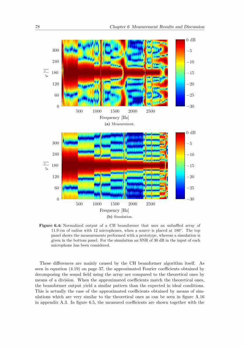
78 Chapter 6 Measurement Results and Discussion
(a) Measurement.
(b) Simulation.
Figure 6.4: Normalized output of a CH beamformer that uses an unbaffled array of11.9 cm of radius with 12 microphones, when a source is placed at 180∘. The toppanel shows the measurements performed with a prototype, whereas a simulation isgiven in the bottom panel. For the simulation an SNR of 30 dB in the input of eachmicrophone has been considered.
These differences are mainly caused by the CH beamformer algorithm itself. Asseen in equation (4.19) on page 37, the approximated Fourier coefficients obtained bydecomposing the sound field using the array are compared to the theoretical ones bymeans of a division. When the approximated coefficients match the theoretical ones,the beamformer output yield a similar pattern than the expected in ideal conditions.This is actually the case of the approximated coefficients obtained by means of sim-ulations which are very similar to the theoretical ones as can be seen in figure A.16in appendix A.3. In figure 6.5, the measured coefficients are shown together with the

6.2 Beamformers Output 79
theoretical ones. In contrast to the case of the simulations, it can be seen that the the-oretical and the measured coefficients are not completely similar, and hence differencesbetween the expected and the measured outputs are observed in figure 6.4. At thispoint it should be emphasized that the number of orders used for the CH beamformercalculation follows N = ⌈kR⌉. In this sense, the high deviations at low frequencies fororders higher than two, due to the presence of background noise, should not be takeninto account for the comparison since these orders are not used for the algorithm atsuch frequencies. In the frequency range where each order is used, it can be seen thatall approximated coefficients present some ripples that are not present in the theoreticalcase, but in general they follow the same tendency. The most remarkable difference isobserved at the dip obtained for the first order as it does not coincide with the theo-retical case, see panel (b). In fact, this is the cause that makes the output shown infigure 6.4 present unresolved frequencies in a relatively wide frequency range around1.7 kHz.
The differences between measurements and simulations can be further examined bystudying the resolution and the MSL. These quantities are shown in figure 6.6. Theresolution is very similar to the one obtained with the simulation. It can be seen thatthe response follows the simulation curve rather accurately and even those frequenciesthat present singularities practically coincide. Just small deviations can be observed atthe lowest frequencies, which are attributed to the influence of background noise.
In contrast with the resolution, the MSL deviates somewhat from the simulation. Ingeneral, this measure is higher than the expected one and worsens in the surroundingsof the singularities. Besides, it is rather high at frequencies below 100 Hz, though thisis not a problem since these frequencies are not required for the performance of thearray. These deviations from the theoretical case are mainly related to, on the onehand, the influence of background noise and, on the other hand, the difference betweenthe measured Fourier coefficients and the theoretical ones. For example, it can be seenthat the ripples at around 300 Hz and 450 Hz coincide completely with the deviationsbetween the measured coefficient of order zero and the theoretical one in the samefrequency range.
In chapter 5, it was observed that CHB is rather vulnerable to noise, and this canparticularly be seen in the MSL as it is more sensitive measure than the resolution. Inaddition to this, it can also be stated that the MSL is highly affected by the differencesbetween the measured Fourier coefficients and the expected ones.
In figure 6.7, the normalized output obtained with the DS beamformer is shown. Ascan be seen, the results agree very well with the theoretical ones. This is also observedwith the resolution and the MSL which are provided in figure 6.8. There are only a fewdifferences compared with the simulations. The first one is that the resolution equals360∘, meaning that the main lobe is omnidirectional, up to a frequency 20 Hz higherthan expected, see panel (a). The second difference is that the first side lobe appearsat 634 Hz instead of 556 Hz as obtained in the simulation, see panel (b). The last maindifference is that the MSL is better than expected in the range from 1950 Hz to about2300 Hz. These differences are again mainly attributed to the differences between themeasured Fourier coefficients and the theoretical ones. However, the beampattern aswell as the resolution and the MSL, are not that affected by these differences like inthe case of CHB. This proves again that DSB is a more robust algorithm.

80 Chapter 6 Measurement Results and Discussion
Frequency [Hz]
Norm
alized∣C
0∣2
[dB]
100 1000−80
−60
−40
−20
0
(a) n = 0
Frequency [Hz]
Norm
alized∣C
1∣2
[dB]
100 1000−80
−60
−40
−20
0
(b) n = 1
Frequency [Hz]
Norm
alized∣C
2∣2
[dB]
100 1000−80
−60
−40
−20
0
(c) n = 2
Frequency [Hz]
Norm
alized∣C
3∣2
[dB]
100 1000−80
−60
−40
−20
0
(d) n = 3
Frequency [Hz]
Norm
alized∣C
4∣2
[dB]
100 1000−80
−60
−40
−20
0
(e) n = 4
Frequency [Hz]
Norm
alized∣C
5∣2
[dB]
100 1000−80
−60
−40
−20
0
(f) n = 5
Figure 6.5: Comparison between the theoretical Fourier coefficients (dashed line) and theapproximated Fourier coefficients measured with an array of 11.9 cm of radius and12 microphones (continuous line).

6.2 Beamformers Output 81
Frequency [Hz]
RESCH[∘]
MeasurementSimulation
100 10000
60
120
180
240
300
360
(a)
Frequency [Hz]
MSLCH[dB]
MeasurementSimulation
100 1000−20
−15
−10
−5
0
(b)
Figure 6.6: Resolution and MSL of a CH beamformer that uses an unbaffled array of11.9 cm of radius with 12 microphones, when a source is placed at 180∘. The theo-retical case obtained by means of a simulation is also displayed. The SNR in eachmicrophone has been set to 30 dB for the simulation.

82 Chapter 6 Measurement Results and Discussion
(a) Measurement.
(b) Simulation.
Figure 6.7: Normalized output of a DS beamformer that uses an unbaffled array of11.9 cm of radius with 12 microphones, when a source is placed at 180∘. The toppanel shows the measurements performed with a prototype, whereas a simulation isgiven in the bottom panel. For the simulation an SNR of 30 dB in the input of eachmicrophone has been considered.

6.2 Beamformers Output 83
Frequency [Hz]
RESDS[∘]
MeasurementSimulation
100 10000
60
120
180
240
300
360
(a)
Frequency [Hz]
MSLDS[dB]Sim
MeasurementSimulation
100 1000−50
−40
−30
−20
−10
0
(b)
Figure 6.8: Resolution and MSL of a DS beamformer that uses an unbaffled array of11.9 cm of radius with 12 microphones, when a source is placed at 180∘. The theo-retical case obtained by means of a simulation is also displayed. The SNR in eachmicrophone has been set to 30 dB for the simulation.

84 Chapter 6 Measurement Results and Discussion
6.3 Repeatability of the Measurements
In order to analyze the repeatability of the measurements, ten consecutive measure-ments have been performed with the same conditions. The source has been placed at180∘ with respect to the array, at a distance of 4.6 m like in the measurements of theprevious section.
Each measurement has been recorded for 2 s, which corresponds to two periods of thegenerator signal, and has been averaged afterwards over the periods in order to lowerthe influence of the background noise. The equivalent sound level pressure of the signalsat each channel is in average 70.1 dB SPL, and the estimated noise is 32.7 dB SPL. Ineach measurement the resolution and the MSL have been calculated with both CHB andDSB. The mean values and the standard deviation of these two measures is analyzedin the following.
In figure 6.9, the mean and the standard deviation of the resolution are shown. As canbe seen, the mean curves obtained with the two techniques are very similar to the resultsshown in the previous section where the measurements have been compared to thesimulations. For this reason, a separate discussion between the mean and the theoreticalvalues would be redundant. However, the present results can be seen together with theexpected ones in figure A.14 in appendix A.3.
Regarding the standard deviation in the case of CHB, some deviations can be ob-served at frequencies around 100 Hz due to the presence of background noise. At 150 Hzand 250 Hz higher deviations can be observed which are attributed to the influence ofthe electrical noise (or hum), since these components are placed at odd harmonics of itsfundamental frequency (50 Hz). At higher frequencies the deviation is rather small withexception of several peaks that correspond to the singularities due to the unresolvedfrequencies in the Fourier coefficients. The vicinity of these frequencies also presentssmall variation.
When dealing with DSB, the higher deviations are found around 257 Hz and 280 Hzwhich coincide with the beginning of the decrease of the resolution. In addition, smallerdeviations can be seen up to 350 Hz. Apart from these deviations, the influence of thehum is also seen through the relatively small peaks at 350 Hz, 450 Hz, 550 Hz, 650 Hzand 750 Hz.
The mean and the standard deviation of the MSL are shown in figure 6.10. In the caseof CHB, the deviation is in general fairly small (less than 0.25 dB) except at the lowestfrequencies and at some isolated peaks. While the variation at lower frequencies is dueto background noise, most of the peaks are the consequence of either the influence ofthe unresolved frequencies due to the Fourier coefficients or the hum since they appearat odd harmonics of its fundamental frequency.
In general terms, the deviation of the MSL for DSB is smaller than in CHB. Thelarger variation is found at those frequencies where a side lobe appears for the firsttime, around 627 Hz and 660 Hz. Also with DSB the influence of the hum is observed.
In conclusion, from these results it is seen that with CHB the results present morevariation than with DSB due to the fact that it is less robust with respect to noise.
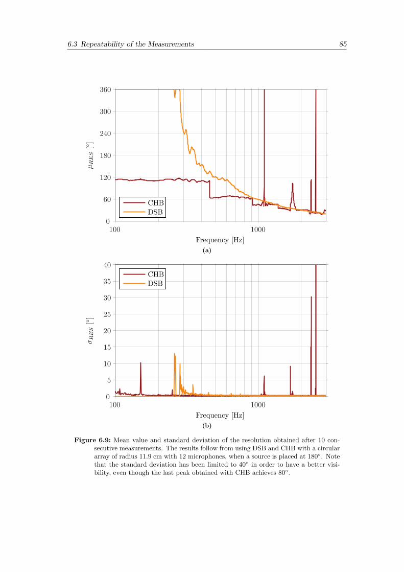
6.3 Repeatability of the Measurements 85
Frequency [Hz]
�RES[∘]
CHBDSB
100 10000
60
120
180
240
300
360
(a)
Frequency [Hz]
�RES[∘]
CHBDSB
100 10000
5
10
15
20
25
30
35
40
(b)
Figure 6.9: Mean value and standard deviation of the resolution obtained after 10 con-secutive measurements. The results follow from using DSB and CHB with a circulararray of radius 11.9 cm with 12 microphones, when a source is placed at 180∘. Notethat the standard deviation has been limited to 40∘ in order to have a better visi-bility, even though the last peak obtained with CHB achieves 80∘.
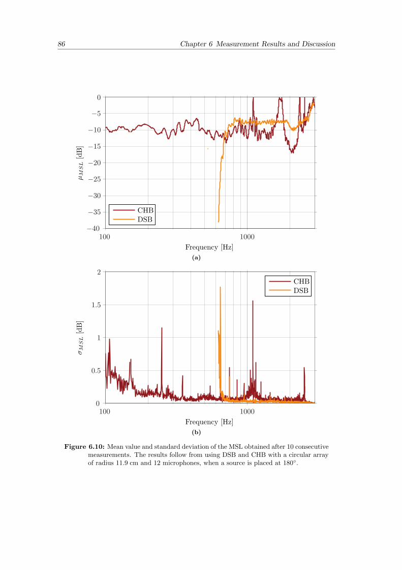
86 Chapter 6 Measurement Results and Discussion
Frequency [Hz]
�M
SL[dB]
CHBDSB
100 1000−40
−35
−30
−25
−20
−15
−10
−5
0
(a)
Frequency [Hz]
�M
SL[dB]
CHBDSB
100 10000
0.5
1
1.5
2
(b)
Figure 6.10: Mean value and standard deviation of the MSL obtained after 10 consecutivemeasurements. The results follow from using DSB and CHB with a circular arrayof radius 11.9 cm and 12 microphones, when a source is placed at 180∘.

6.4 Influence of the Distance between Source and Array 87
6.4 Influence of the Distance between Source and Array
The influence of the distance between the source and the array is analyzed in thissection. The source, initially placed 4.6 m away from the array as in the previousexperiment, has been moved back and forth to different positions by means of a railhanging from the ceiling. In all cases, the source is on-axis with respect to the array,i. e. at 0∘.
The generator signal has been kept constant along the measurements. The signalcaptured by the microphones has been recorded during 2 s, which corresponds to twoperiods of the generator signal, and has been averaged over the number of periods. Thesound pressure level in the microphones as well as the distance between the source andthe array are stated in table 6.1. The sound pressure level of the background noise atthe microphones is 32.8 dB SPL in average.
Table 6.1: Distance d between the source and the array at each position with the corre-sponding sound pressure level captured at the microphones in average.
# Position d [m] Leq,m [dB SPL]
1 2.6 75.82 3.6 72.93 4.6 70.94 5.6 69.4
The resolution and the MSL obtained with these configurations are shown in fig-ures 6.11 and 6.12 for CHB and DSB, respectively.
In the case of CHB, the resolution is very similar for all distances between arrayand source. The exception is found at those frequencies that are not resolved with theFourier coefficients. As can be seen the resolution worsens with increasing distance.When DSB is used, the resolution is practically the same at high frequencies, whereassome differences are seen in the beginning of the decay of the resolution until 600 Hz.
Although the MSL curves for all cases follow the same tendency with both techniques,they do not coincide exactly as this measure is quite sensitive to background noise asmentioned in the previous sections. In this sense, the equivalent sound pressure levelof the signal decreases with increasing distance, as shown in table 6.1. This in turncauses the SNR to worsen, and therefore the resulting resolution and MSL suffer morevariation. This effect can also be seen in the case of DSB, through some ‘unexpected’side lobes that appear between 500 Hz and 600 Hz for the longer distances, due to thelow SNR in these measurements.
It is interesting to analyze whether the assumption of far-field is fulfilled with thedistances of concern. A common rule of thumb for the approximate distance at whichthe far-field approximation is valid follows d ≫ �. Even though this is not fulfilled atthe very low frequencies when the distance is 2.6 m, the far-field assumption seems tobe still valid since the results have the same tendency as the ones obtained with longerdistances.
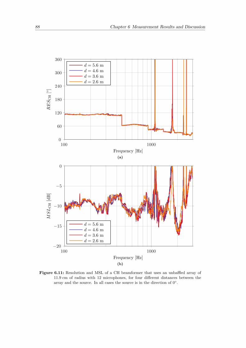
88 Chapter 6 Measurement Results and Discussion
Frequency [Hz]
RESCH[∘]
d = 5.6 md = 4.6 md = 3.6 md = 2.6 m
100 10000
60
120
180
240
300
360
(a)
Frequency [Hz]
MSLCH[dB]
d = 5.6 md = 4.6 md = 3.6 md = 2.6 m
100 1000−20
−15
−10
−5
0
(b)
Figure 6.11: Resolution and MSL of a CH beamformer that uses an unbaffled array of11.9 cm of radius with 12 microphones, for four different distances between thearray and the source. In all cases the source is in the direction of 0∘.
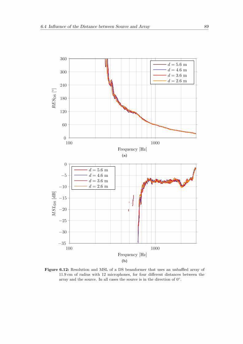
6.4 Influence of the Distance between Source and Array 89
Frequency [Hz]
RESDS[∘]
d = 5.6 md = 4.6 md = 3.6 md = 2.6 m
100 10000
60
120
180
240
300
360
(a)
Frequency [Hz]
MSLDS[dB]
d = 5.6 md = 4.6 md = 3.6 md = 2.6 m
100 1000−35
−30
−25
−20
−15
−10
−5
0
(b)
Figure 6.12: Resolution and MSL of a DS beamformer that uses an unbaffled array of11.9 cm of radius with 12 microphones, for four different distances between thearray and the source. In all cases the source is in the direction of 0∘.

90 Chapter 6 Measurement Results and Discussion
6.5 Influence of Background Noise
In the previous sections it has been observed that the resolution and particularly theMSL are influenced by background noise. In this section, further analysis is done bycomparing four situations where the SNR at the array microphones is different. Forthese measurements, the source is placed on-axis with the array at a distance of 4.6 m.In each measurement, the signals captured by microphones have been recorded for 2 sand averaged over two periods, which is the number of periods used in the generatorsignal. The sound pressure level of the background noise in each channel is estimatedto be 31.9 dB SPL, in mean. The level of the generator signal has been varied bymeans of the amplifier at each measurement. The resulting sound pressure level at themicrophones and the corresponding SNR are shown in table 6.2.
The resolution and the MSL obtained from the measurements are depicted in fig-ures 6.13 and 6.14 for CHB and DSB. Obviously, these measures worsen when theSNR decreases, with both techniques. In the case of CHB, the influence of backgroundnoise is stronger at low frequencies as can be seen from the resolution and MSL. As an-alyzed in section 5.3.2.2, this is mainly caused by the CHB algorithm, since it amplifiesthe noise when multiplying with the terms 1/Cn shown in figure 5.14 on page 61. Athigh frequencies, these terms do not affect the CH beamformer output, and hence theresolution is rather independent of the SNR.
For DSB, the resolution presents more variation at those frequencies that correspondto the beginning of the decay, between 100 Hz and 600 Hz. At higher frequencies allsituations yield practically the same resolution.
The MSL with CHB is polluted with background noise in a wider frequency rangethan the resolution and also worsen considerably with decreasing SNR. By contrast,with DSB even with the lowest SNR the result is acceptable. The effect of noise in theMSL when dealing with DSB is mainly seen in the ‘unexpected’ side lobes that appearin the range between 500 Hz and 600 Hz, when the SNR worsens.
With the above ideas two main conclusions can be drawn. On the one hand it hasbeen seen that DSB is more robust to background noise than CHB. On the other handthe MSL appears to be more vulnerable than the resolution with respect to backgroundnoise.
Table 6.2: Averaged sound pressure level at the input of the microphones and estimatedSNR for each measurement.
# Measurement Leq,m[dB SPL] SNR [dB]
1 43.3 11.42 55.1 23.23 65.5 33.64 73.5 41.6

6.5 Influence of Background Noise 91
Frequency [Hz]
RESCH[∘]
SNR = 11.4 dBSNR = 23.2 dBSNR = 33.6 dBSNR = 41.6 dB
100 10000
60
120
180
240
300
360
(a)
Frequency [Hz]
MSLCH[dB]
SNR = 11.4 dBSNR = 23.2 dBSNR = 33.6 dBSNR = 41.6 dB
100 1000−25
−20
−15
−10
−5
0
(b)
Figure 6.13: Resolution and MSL of a CH beamformer that uses an unbaffled array of11.9 cm of radius with 12 microphones, for four different SNR. In all cases thesource is in the direction of 0∘ at 4.6 m away from the array.

92 Chapter 6 Measurement Results and Discussion
Frequency [Hz]
RESDS[∘]
SNR = 11.4 dBSNR = 23.2 dBSNR = 33.6 dBSNR = 41.6 dB
100 10000
60
120
180
240
300
360
(a)
Frequency [Hz]
MSLDS[dB]
SNR = 11.4 dBSNR = 23.2 dBSNR = 33.6 dBSNR = 41.6 dB
100 1000−50
−40
−30
−20
−10
0
(b)
Figure 6.14: Resolution and MSL of a DS beamformer that uses an unbaffled array of11.9 cm of radius with 12 microphones, for four different SNR. In all cases thesource is in the direction of 0∘ at 4.6 m away from the array.

6.6 Angle Discrimination 93
6.6 Angle Discrimination
In this section, the array performance is to be analyzed over 360∘. The source is keptat the same position along the measurements at 4.6 m away from the array. For thefirst measurement, the array is focused towards the source, i. e. on-axis, and is rotatedby 10∘ after each measurement until reaching 360∘. In this way, 36 different directionsof the source with respect to the array are measured. The signals captured by thearray microphones are recorded for 2 s and averaged by two, which is the number ofperiods of the generator signal. The averaged sound pressure level of the signals at eachmicrophone is 71 dB SPL, whereas the background noise is estimated to be 33 dB SPLduring the measurements.
According to the simulations shown in sections 5.3.2.1 and 5.3.3.1, in ideal conditionsthe resolution and the MSL are independent of the source position at low frequencies,whereas at higher frequencies small periodic fluctuations are observed. Furthermore,these fluctuations increase with increasing frequency.
In figures 6.15 and 6.16, the resolution obtained from the measurements is shownat several frequencies as a function of the angle of the source, for CHB and DSBrespectively.
's [∘]
RESCH[∘]
f = 100 Hz
f = 700 Hz
f = 1 kHz
f = 1.5 kHz
f = 2 kHz
0 30 60 90 120 150 180 210 240 270 300 330 36020
40
60
80
100
120
Figure 6.15: Resolution at five different frequencies as a function of the angular positionof the source obtained with CHB. A circular array of radius of 11.9 cm with 12microphones is used. The source is at a distance of 4.6 m from the array.
As can be seen, the resolution is fairly constant for both CHB and DSB and hence itagrees with the simulations. The small fluctuations that are observed at low frequenciesare mainly attributed to the influence of background noise. At high frequencies, aperiodic pattern is sensed with both techniques.
The MSL obtained with CHB and DSB is shown in figures 6.17 and 6.18. In bothcases, the results are not as constant as expected at the lowest frequencies due to the

94 Chapter 6 Measurement Results and Discussion
's [∘]
RESDS[∘]
f = 700 Hzf = 1 kHzf = 1.5 kHzf = 2 kHz
0 30 60 90 120 150 180 210 240 270 300 330 36020
40
60
80
100
120
Figure 6.16: Resolution at five different frequencies as a function of the angular positionof the source obtained with DSB. A circular array of radius of 11.9 cm with 12microphones is used. The source is at a distance of 4.6 m from the array.
's [∘]
MSLCH[dB]
f = 100 Hzf = 700 Hzf = 1 kHzf = 1.5 kHzf = 2 kHz
0 30 60 90 120 150 180 210 240 270 300 330 360−16
−14
−12
−10
−8
−6
−4
Figure 6.17: MSL at five different frequencies as a function of the angular position ofthe source obtained with CHB and a circular array with radius of 11.9 cm and 12microphones. The source is at a distance of 4.6 m from the array.
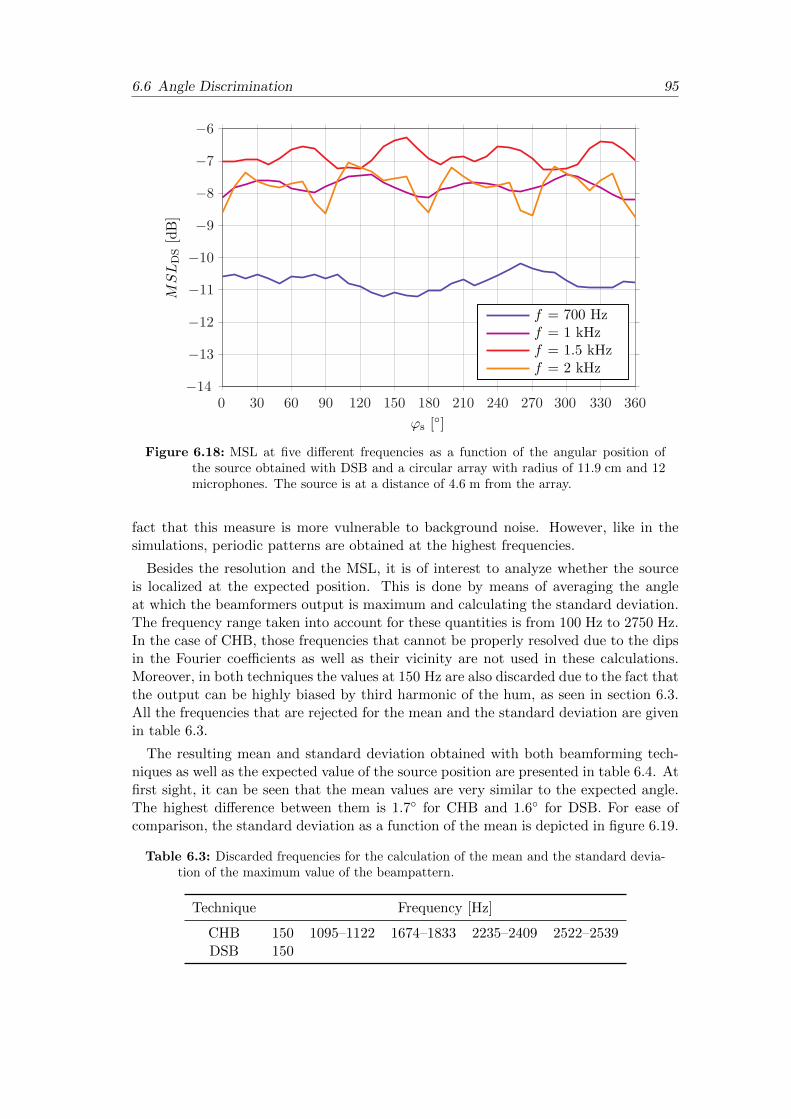
6.6 Angle Discrimination 95
's [∘]
MSLDS[dB]
f = 700 Hzf = 1 kHzf = 1.5 kHzf = 2 kHz
0 30 60 90 120 150 180 210 240 270 300 330 360−14
−13
−12
−11
−10
−9
−8
−7
−6
Figure 6.18: MSL at five different frequencies as a function of the angular position ofthe source obtained with DSB and a circular array with radius of 11.9 cm and 12microphones. The source is at a distance of 4.6 m from the array.
fact that this measure is more vulnerable to background noise. However, like in thesimulations, periodic patterns are obtained at the highest frequencies.
Besides the resolution and the MSL, it is of interest to analyze whether the sourceis localized at the expected position. This is done by means of averaging the angleat which the beamformers output is maximum and calculating the standard deviation.The frequency range taken into account for these quantities is from 100 Hz to 2750 Hz.In the case of CHB, those frequencies that cannot be properly resolved due to the dipsin the Fourier coefficients as well as their vicinity are not used in these calculations.Moreover, in both techniques the values at 150 Hz are also discarded due to the fact thatthe output can be highly biased by third harmonic of the hum, as seen in section 6.3.All the frequencies that are rejected for the mean and the standard deviation are givenin table 6.3.
The resulting mean and standard deviation obtained with both beamforming tech-niques as well as the expected value of the source position are presented in table 6.4. Atfirst sight, it can be seen that the mean values are very similar to the expected angle.The highest difference between them is 1.7∘ for CHB and 1.6∘ for DSB. For ease ofcomparison, the standard deviation as a function of the mean is depicted in figure 6.19.
Table 6.3: Discarded frequencies for the calculation of the mean and the standard devia-tion of the maximum value of the beampattern.
Technique Frequency [Hz]
CHB 150 1095–1122 1674–1833 2235–2409 2522–2539DSB 150

96 Chapter 6 Measurement Results and Discussion
Table 6.4: Localization of the source direction with CHB and DSB. The first column givesthe expected angle of the source with respect to the center of the array, whereas theother columns provide the mean and standard deviation for each technique. All unitsare degrees.
Expected 'sCHB DSB
�' �' �' �'
0 0.3 0.79 0.4 0.7510 10.6 1.05 11.0 0.9120 20.5 1.86 20.3 0.7730 30.4 0.97 30.7 0.7940 40.5 1.29 41.0 0.8650 51.3 1.35 51.0 0.8460 61.0 0.98 61.1 0.8470 70.4 1.71 70.8 0.8580 80.6 1.20 80.3 0.9290 90.7 0.91 90.8 0.84100 100.2 1.21 100.5 0.95110 110.9 1.92 110.5 0.85120 120.2 1.21 120.3 0.86130 130.2 1.44 130.6 0.87140 141.1 1.44 140.7 0.88150 150.7 1.01 150.6 0.86160 161.1 1.74 161.4 0.88170 171.6 1.21 171.3 0.95180 180.4 0.87 180.6 0.83190 190.4 1.16 190.9 0.96200 201.6 1.89 201.4 0.85210 210.8 1.07 211.2 0.84220 221.1 1.27 221.6 0.82230 231.7 1.33 231.4 0.86240 241.1 0.92 241.1 0.82250 251.1 1.68 251.5 0.83260 261.2 1.11 260.8 0.86270 271.5 0.90 271.6 0.82280 281.2 1.12 281.5 0.92290 291.1 1.89 290.8 0.81300 300.9 1.11 301.0 0.81310 310.3 1.39 310.7 0.83320 320.8 1.42 320.4 0.84330 330.5 0.91 330.4 0.83340 340.4 1.77 340.7 0.85350 351.5 1.20 351.1 0.90360 359.6 0.88 359.7 0.83

6.7 Array Performance with Two Sources 97
�' [∘]
�'[∘]
CHBDSB
0 30 60 90 120 150 180 210 240 270 300 330 3600
0.5
1
1.5
2
Figure 6.19: Standard deviation as a function of the mean of the direction where thesource is localized. These two measures are the result of averaging and calculatingthe standard deviation of the angles where the beamformers present the maximumoutput over all the frequency range of interest, i. e. 100 Hz to 2750 Hz, with theexception of those frequencies stated in table 6.3.
The results reveal that the standard deviation using DSB is always smaller than theone obtained with CHB: it is within the range between 0.75∘ and 0.95∘ for DSB andbetween 0.75∘ and 1.9∘ for CHB. Therefore, for DSB the standard deviation is ratherindependent of the position of the source. When dealing with CHB a ‘periodic’ patternof 90∘ can be seen. This pattern alternates between minima at multiples of 30∘ andmaxima in between. Note that the minima coincide with positions of the microphones inthe array, which means that with CHB the source can be localized with better accuracywhen it is placed in the direction of the array microphones. The fact that the standarddeviation is lower with DSB than with CHB proves once more the robustness of theformer technique.
6.7 Array Performance with Two Sources
The last experiment deals with the beamformers behavior when two uncorrelatedsources are present. To do so, another loudspeaker, a Dynaudio Acoustics BM 6A, isplaced in the anechoic room apart from the spherical source. It is fed by the generatorof a portable Bruel & Kjær PULSE Analyzer. The generator signal consists in pseu-dorandom noise with frequency content up to 3.2 kHz, resolution of 1 Hz and period of1 s, as in the case of the signal used for the spherical loudspeaker (see section 6.1). Theuse of two generators of pseudorandom noise makes the signals of the loudspeakers tobe uncorrelated. This is actually a premise for the proper localization of both sources.
Both speakers are placed at about 4.6 m from the center of the array. While theposition of the loudspeaker mounted on a sphere is kept at 180∘ throughout the mea-

98 Chapter 6 Measurement Results and Discussion
surements, the other loudspeaker is placed in the directions: 174∘, 151∘, 119∘ and 290∘.In this way, both sources are really close to each other in the beginning, and they areprogressively getting farther away in the consecutive measurements.
The speakers present a similar sound pressure level at the array when they are drivenindependently from each other: 70 dB SPL in the case of the spherical source and70.2 dB SPL for the loudspeaker BM 6A. The sound pressure level due to backgroundnoise is about 33 dB SPL. These values are obtained after recording the signal during2 s and averaging over two periods, which corresponds to the number of periods of thegenerators signal.
The resulting sound field created by both sources being active is captured by the arraymicrophones, recorded during 2 s and averaged over two afterwards. The normalizedbeamformer outputs obtained from each measurement when CHB is used are shown infigure 6.20.
(a) 's2 = 174∘; Δ' = 6∘. (b) 's2 = 151∘; Δ' = 29∘.
−30
−25
−20
−15
−10
−5
0 dB
(c) 's2 = 119∘; Δ' = 61∘. (d) 's2 = 290∘; Δ' = 110∘.
−30
−25
−20
−15
−10
−5
0 dB
Figure 6.20: Normalized output of a CH beamformer that uses an unbaffled array ofradius 11.9 cm with 12 microphones, when two uncorrelated sources are present.The sources are placed 4.6 m away from the array. While one of them is kept at180∘ through all the measurements, the other one is moved to 174∘, 151∘, 119∘
and 290∘.

6.7 Array Performance with Two Sources 99
In panel (a), the angular distance between the sources is only Δ' = 6∘, and as canbe seen the beamformer cannot resolve them at all. In panel (b), the beamformercan distinguish between both sources just at really high frequencies. With increasingangular distance between the sources, the beamformer can progressively resolve themin a wider frequency range as shown in panels (c) and (d).
According to section 4.5.1, the definition of the resolution coincides with the minimumdistance between to incoherent sources in order for them to be distinguished. It isinteresting to see how this is fulfilled in the present experiment. For example, in thefrequency range of concern, the resolution is never equal or inferior than 6∘ as seen infigure 6.6 or as stated in table 5.2 on page 72. Therefore, with a distance of Δ' = 6∘
it is not possible to resolve between both sources as observed from figure 6.20. WhenΔ' = 29∘, they can be resolved at those frequencies where the resolution is equal orsmaller than 29∘. Actually this occurs in the range from about 2.2 kHz up to 2.7 kHzas the resolution is 22∘ approximately. For each angular distance Δ', table 6.5 stateswhen this value is equal to or smaller than the resolution and the expected frequencyrange where it occurs.
In this table, it can be seen that the frequency ranges in which the beamformer isexpected to resolve the sources depending on the angular difference between them agreevery well with the results shown in figure 6.20.
Table 6.5: Frequency range in which the CH beamformer can distinguish between twosources for a given angular difference Δ' between them, according to the resolutioncriterion.
FrequencyResolution
Δ'range 6∘ 29∘ 61∘ 110∘
100–458 Hz 112∘ 7 7 7 7
450–917 Hz 65∘ 7 7 7 3
918–1376 Hz 46∘ 7 7 3 3
1377–1834 Hz 36∘ 7 7 3 3
1835–2293 Hz 31∘ 7 7 3 3
2294–2752 Hz 22∘ 7 3 3 3
Figure 6.21 shows the beampatterns obtained with DSB. As can be seen, the resultsshow the same tendency as in the case of CHB, that is, with increasing angular distancethe beamformer is able to resolve the sources in a wider frequency range. However, thefrequency range is equal or smaller than in the case of CHB, since unlike CHB, the DSbeamformer is omnidirectional at low frequencies.
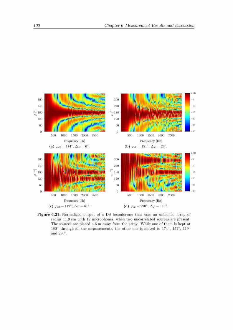
100 Chapter 6 Measurement Results and Discussion
(a) 's2 = 174∘; Δ' = 6∘. (b) 's2 = 151∘; Δ' = 29∘.
−30
−25
−20
−15
−10
−5
0 dB
(c) 's2 = 119∘; Δ' = 61∘. (d) 's2 = 290∘; Δ' = 110∘.
−30
−25
−20
−15
−10
−5
0 dB
Figure 6.21: Normalized output of a DS beamformer that uses an unbaffled array ofradius 11.9 cm with 12 microphones, when two uncorrelated sources are present.The sources are placed 4.6 m away from the array. While one of them is kept at180∘ through all the measurements, the other one is moved to 174∘, 151∘, 119∘
and 290∘.

7Conclusions
7.1 Summary and Conclusions
The localization of environmental noise sources has been investigated with two dif-ferent beamforming techniques applied to circular arrays. These are a new techniquecalled Circular Harmonics beamforming and the well-known Delay-and-Sum beamform-ing. One of the main contributions of this work is the complete description of thesetechniques given in chapter 4. CHB is an adaptation of the Spherical Harmonics beam-forming technique to a circular geometry. It is based on the decomposition of thesound field into a series of harmonics, using the principles of the Fourier series. DSBis typically implemented in the time domain. However, in the present work it has beendeveloped in the frequency domain by using matched field processing. The latter makesit possible to use the concepts of the decomposition of the sound field as in CHB.
Concerning the real implementation of these beamformers, two main sources of errorarise: the truncation error and the sampling error. The truncation error is due to thefact that a finite number of orders is used for the decomposition of the sound field, whenin theory an infinite number of orders should be taken into account. The second errorresults from the decomposition of the sound field based on the information measured atdiscrete points. The effect of these errors has been analyzed in chapter 3. It has beenshown that they can be minimized when the number of orders follows N = ⌈kR⌉ andthe number of array microphones exceeds twice the number of orders, i. e. M > 2 ⌈kR⌉.
Environmental noise sources are broadband sources, and hence, an array used fortheir localization must have a wide operating frequency range. After several measure-ments, it turns out that an array that covers the range from 100 Hz to about 2.5 kHzis reasonable, since this range represents the major spectral content of the sources ofinterest. In addition, the array is required to have a maximum radius of 20 cm as it ismeant to be portable, and has to be conformed by a moderate number of microphones.Taking these constraints into account, the performance of circular arrays using CHBand DSB has been simulated and evaluated by means of two measures, the resolution
101
102 Chapter 7 Conclusions
and the MSL.
The following conclusions can been drawn from the simulation results:
� For both CHB and DSB, the larger the radius of the array, the better the per-formance. In addition, the overall performance also improves with increasingfrequency.
� For a given array, CHB has better resolution and MSL in a wider frequency rangethan in the case of DSB.
� The frequency range is limited at low frequencies by the influence of backgroundnoise in the case of CHB and by the fact that the output is omnidirectional forDSB. At high frequencies the limitation is given by the increase of the samplingerror, in both cases.
� In the presence of background noise, DSB is more robust than CHB. Besides, theresolution is less contaminated than the MSL.
� CH beamformers present singularities, i. e. frequencies that cannot properly beresolved, when unbaffled circular arrays are used. This problem would be solvedif it were feasible to mount the arrays on rigid cylindrical baffles of infinite length.
� The performance of DS beamformers would improve considerably by mounting thearrays on rigid cylindrical baffles of infinite length, but as mentioned previously,this is an unrealistic solution.
� It has been proved that the number of orders used for the beamforming algorithmsis optimum when it follows N = ⌈kR⌉ for CHB, and N = ⌈kR⌉+ 1 for DSB.
The results of the simulations reveal that the performance considerably improvesjust by mounting the array on a rigid cylindrical baffle of infinite length, though itis obvious that in real implementations the length of the cylindrical baffle must befinite. In chapter 3, an approximation of a cylinder of infinite length using a finitelength cylinder given in the literature has been further examined. Unfortunately, theresults have shown that this approximation is not really reliable. Consequently, anunbaffled array has been proposed for the implementation of a prototype. Consideringthe results of the simulations and the requirements previously mentioned, it has beenrecommended to use a radius of about 10 cm and 11 microphones.
The final prototype, with a radius of 11.9 cm and 12 microphones, has been tested inanechoic conditions. Very satisfactory results have been obtained as the beampatterns,the resolution and the MSL present extremely good agreement with the simulations,for both CHB and DSB.
Therefore, we can assert that the proposal of such prototype used in combinationwith the designed beamforming techniques for the localization of environmental noisesources is not only feasible but also very effective in terms of resolution and MSL, inmost of the frequency range of interest. In this sense, it is recommended to use CHB forall the frequency range with exception of those high frequencies that cannot be properlyresolved due to the nature of this technique. At such frequencies, it is convenient to useDSB instead. In addition to this, DSB should not be underestimated in environmentswith poor SNR due to its robustness.

7.2 Future Work 103
Finally, it must be pointed out that even though the array has been designed for thelocalization of environmental noise sources, this work can be used as a guideline forother scenarios where circular arrays are applicable.
7.2 Future Work
The fact that the prototype yields successful results could encourage us to work forthe improvement of such device. The following suggestions for further work are given:
� It has been seen that by mounting the array on a rigid cylindrical baffle of infinitelength the output using DSB improves significantly compared to the unbaffledcase. In fact, just by mounting the array on the infinite baffle, the performance isvery similar to the one of an unbaffled array with twice the radius of the baffledarray. In other words, the baffled array appears to be twice as large as an unbaffledarray with the same radius. For real implementations the length of the cylindricalbaffle must be finite, but it would be very convenient to find which length couldbe regarded as infinite. In chapter 3, an approximation given in the literaturehas been found not to be reliable. For this reason, it would be very useful andchallenging to find an appropriate approximation.
� Although at low frequencies the CH beamformer presents better performancethan the DS beamformer, the resolution is still rather coarse (about 110∘), andhence it gives us a very rough estimation of the direction of the source. In manysituations, it would be desirable to have better accuracy at such low frequencies.However, the only solution taking into account CHB and DSB lays on the designof a larger array, but this does not fulfill the requirements previously mentioned.Therefore, the solutions imply either the use of other beamforming techniquesapplied to circular arrays, or a completely different approach by using other arraygeometries.


AFurther Information
A.1 Bessel Functions
This section provides the characteristics of the Bessel functions frequently used inthis document. All the equations are taken or adapted from [22, 23, 24].
The Bessel’s differential equation of order n ≥ 0 follows
x2∂2w
∂x2+ x
∂w
∂x+(x2 − n2
)w = 0. (A.1)
The general solution to the Bessel’s equation can be written as
w = AJn(x) +BYn(x), (A.2)
where Jn(x) is the Bessel function of the first kind and order n and Yn(x) is theNeumann function (or Bessel functions of the second kind) and order n. The Besselfunctions can be defined as
Jn(x) =1
2�
∫ 2�
0e j(x sin'−n')d'. (A.3)
Alternatively, after applying the change of variable ' = �+�/2 in the previous equation,Jn(x) can be written as follows
Jn(x) =1
2�jn
∫ 2�
0e j(x cos'+n')d'. (A.4)
105
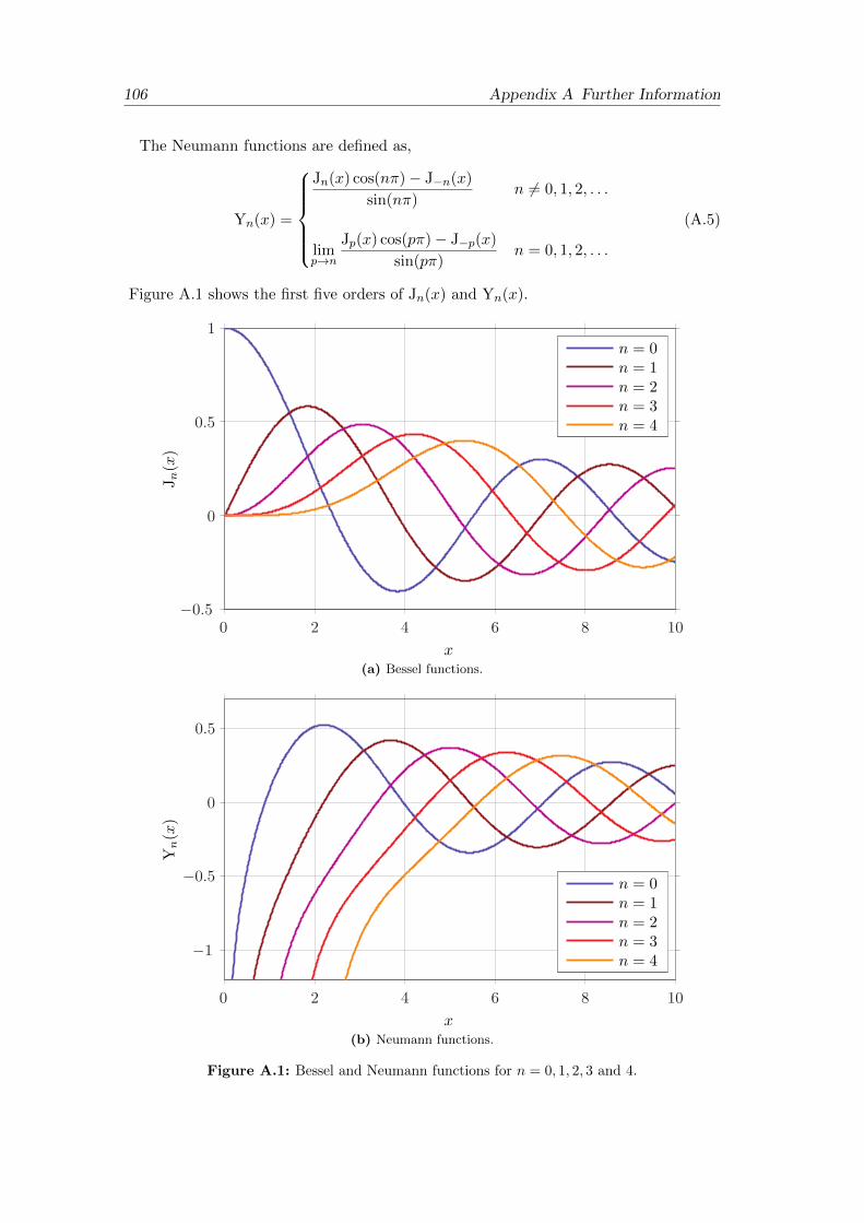
106 Appendix A Further Information
The Neumann functions are defined as,
Yn(x) =
⎧⎨⎩Jn(x) cos(n�)− J−n(x)
sin(n�)n ∕= 0, 1, 2, . . .
limp→n
Jp(x) cos(p�)− J−p(x)
sin(p�)n = 0, 1, 2, . . .
(A.5)
Figure A.1 shows the first five orders of Jn(x) and Yn(x).
x
Jn(x
)
n = 0n = 1n = 2n = 3n = 4
0 2 4 6 8 10−0.5
0
0.5
1
(a) Bessel functions.
x
Yn(x
)
n = 0n = 1n = 2n = 3n = 4
0 2 4 6 8 10
−1
−0.5
0
0.5
(b) Neumann functions.
Figure A.1: Bessel and Neumann functions for n = 0, 1, 2, 3 and 4.
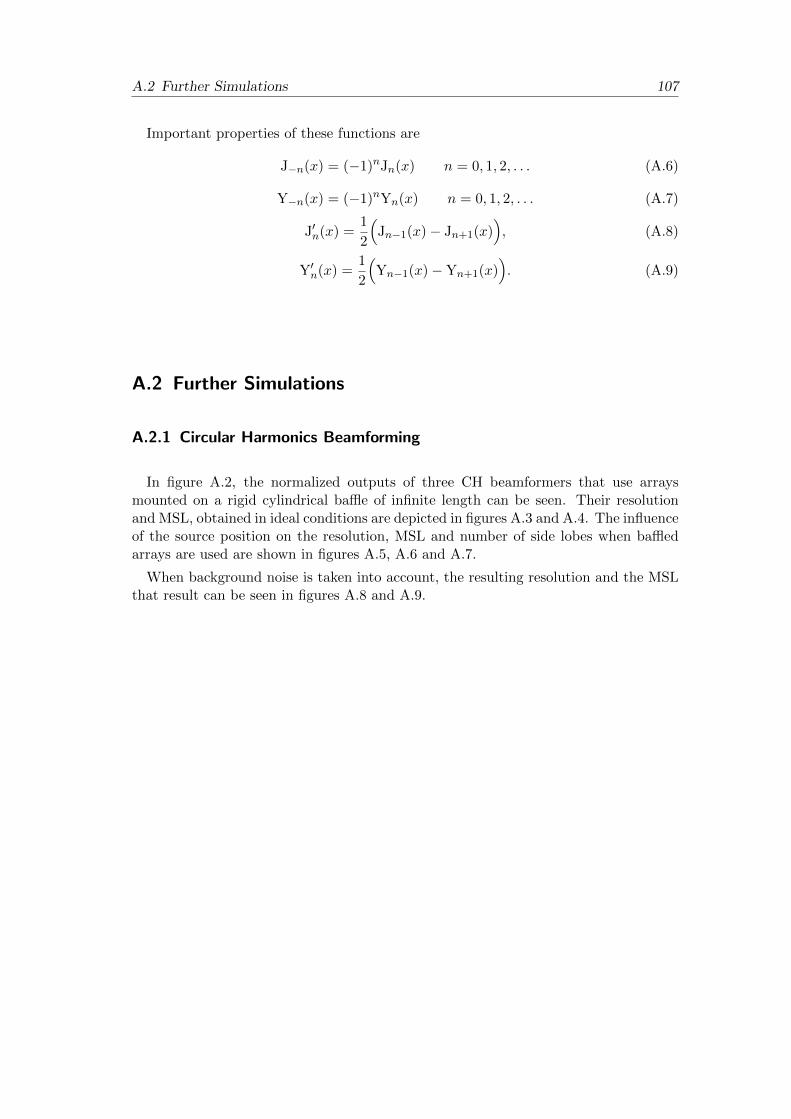
A.2 Further Simulations 107
Important properties of these functions are
J−n(x) = (−1)nJn(x) n = 0, 1, 2, . . . (A.6)
Y−n(x) = (−1)nYn(x) n = 0, 1, 2, . . . (A.7)
J′n(x) =1
2
(Jn−1(x)− Jn+1(x)
), (A.8)
Y′n(x) =1
2
(Yn−1(x)−Yn+1(x)
). (A.9)
A.2 Further Simulations
A.2.1 Circular Harmonics Beamforming
In figure A.2, the normalized outputs of three CH beamformers that use arraysmounted on a rigid cylindrical baffle of infinite length can be seen. Their resolutionand MSL, obtained in ideal conditions are depicted in figures A.3 and A.4. The influenceof the source position on the resolution, MSL and number of side lobes when baffledarrays are used are shown in figures A.5, A.6 and A.7.
When background noise is taken into account, the resulting resolution and the MSLthat result can be seen in figures A.8 and A.9.
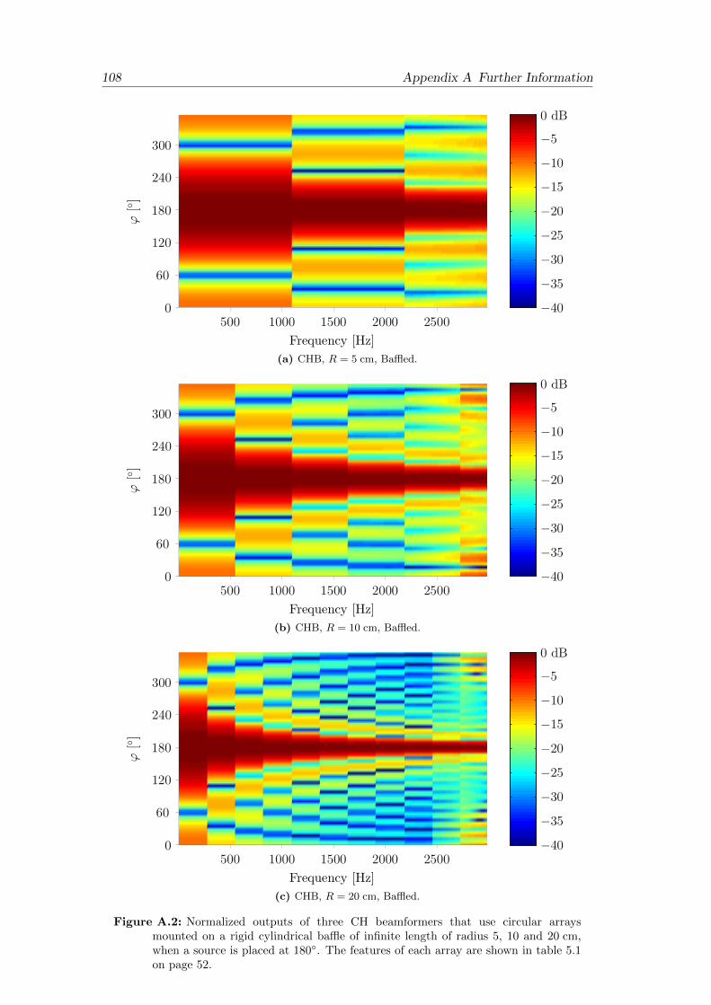
108 Appendix A Further Information
(a) CHB, R = 5 cm, Baffled.
(b) CHB, R = 10 cm, Baffled.
(c) CHB, R = 20 cm, Baffled.
Figure A.2: Normalized outputs of three CH beamformers that use circular arraysmounted on a rigid cylindrical baffle of infinite length of radius 5, 10 and 20 cm,when a source is placed at 180∘. The features of each array are shown in table 5.1on page 52.

A.2 Further Simulations 109
Frequency [Hz]
RESCH[∘]
R = 5 cmR = 10 cmR = 20 cm
100 10000
20
40
60
80
100
120
Figure A.3: Resolution of three CH beamformers that use circular arrays mounted on arigid cylindrical baffle of infinite length of radius 5, 10 and 20 cm, when a source isplaced at 180∘. The features of each array are given in table 5.1.
Frequency [Hz]
MSLCH[dB]
R = 5 cmR = 10 cmR = 20 cm
100 1000−14
−13
−12
−11
−10
−9
−8
−7
Figure A.4: MSL of three CH beamformers that use circular arrays mounted on a rigidcylindrical baffle of infinite length of radius 5, 10 and 20 cm, when a source is placedat 180∘. The features of each array are given in table 5.1 on page 52.

110 Appendix A Further Information
's [∘]
RESCH[∘]
f = 100 Hzf = 700 Hzf = 1.2 kHzf = 2 kHzf = 2.5 kHz
0 60 120 180 240 300 36020
40
60
80
100
120
Figure A.5: Resolution as a function of the angular position of the source obtained withCHB and a circular array mounted on a rigid cylindrical baffle of infinite lengthof radius 10 cm at five different frequencies. The features of the array are given intable 5.1 on page 52.
's [∘]
MSLCH[dB]
f = 100 Hzf = 700 Hzf = 1.2 kHzf = 2 kHzf = 2.5 kHz
0 60 120 180 240 300 360−13
−12.5
−12
−11.5
−11
−10.5
−10
−9.5
Figure A.6: MSL as a function of the angular position of the source obtained with CHBand a circular array mounted on a rigid cylindrical baffle of infinite length of radius10 cm at five different frequencies. The features of the array are given in table 5.1on page 52.

A.2 Further Simulations 111
's [∘]
Number
ofSideLob
es
f = 100 Hzf = 700 Hzf = 1.2 kHzf = 2 kHzf = 2.5 kHz
0 60 120 180 240 300 3600
2
4
6
8
10
Figure A.7: Number of side lobes as a function of the angular position of the sourceobtained with CHB and a circular array mounted on a rigid cylindrical baffle ofinfinite length of radius 10 cm at five different frequencies. The features of thearray are given in table 5.1 on page 52.
Frequency [Hz]
RESCH[∘]
R = 5 cmR = 10 cmR = 20 cm
100 10000
20
40
60
80
100
120
140
Figure A.8: Resolution of three CH beamformers that use circular arrays mounted on arigid cylindrical baffle of infinite length of radius 5, 10 and 20 cm, when a sourceis placed at 180∘ and the SNR in the array microphones is 30 dB. The features ofeach array are given in table 5.1 on page 52.

112 Appendix A Further Information
Frequency [Hz]
MSLCH[dB]
R = 5 cmR = 10 cmR = 20 cm
100 1000−14
−13
−12
−11
−10
−9
−8
−7
Figure A.9: MSL of three CH beamformers that use circular arrays mounted on a rigidcylindrical baffle of infinite length of radius 5, 10 and 20 cm, when a source is placedat 180∘ and the SNR in the array microphones is 30 dB. The features of each arrayare given in table 5.1 on page 52.
A.2.2 Delay-and-Sum Beamforming
The normalized outputs of three DS beamformers that use arrays mounted on a rigidcylindrical baffle of infinite length can be seen in figure A.10. Ideal conditions and asource placed at 180∘ have been considered for these simulations. The influence of thesource position on the resolution and the MSL is shown in figure A.10 for a baffledarray of 10 cm of radius.
The resolution and the MSL of three DS beamformers that use baffled arrays can beseen in figure A.12, when background noise is present.
In figure A.13, the resolution and the MSL are shown for an unbaffled array of 10 cmof radius when 11 and 12 microphones are used.

A.2 Further Simulations 113
(a) DSB, R = 5 cm, Baffled.
(b) DSB, R = 10 cm, Baffled.
(c) DSB, R = 20 cm, Baffled.
Figure A.10: Normalized outputs of three DS beamformers that use circular arraysmounted on a rigid cylindrical baffle of infinite length of radius 5, 10 and 20 cm,when a source is placed at 180∘. The features of each array are shown in table 5.1on page 52.
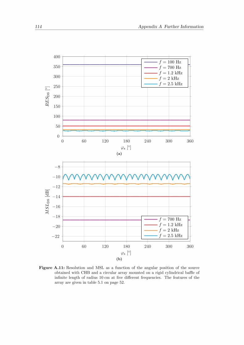
114 Appendix A Further Information
's [∘]
RESDS[∘]
f = 100 Hzf = 700 Hzf = 1.2 kHzf = 2 kHzf = 2.5 kHz
0 60 120 180 240 300 3600
50
100
150
200
250
300
350
400
(a)
's [∘]
MSLDS[dB]
f = 700 Hzf = 1.2 kHzf = 2 kHzf = 2.5 kHz
0 60 120 180 240 300 360
−22
−20
−18
−16
−14
−12
−10
−8
(b)
Figure A.11: Resolution and MSL as a function of the angular position of the sourceobtained with CHB and a circular array mounted on a rigid cylindrical baffle ofinfinite length of radius 10 cm at five different frequencies. The features of thearray are given in table 5.1 on page 52.

A.2 Further Simulations 115
Frequency [Hz]
RESDS[∘]
R = 5 cmR = 10 cmR = 20 cm
100 10000
40
80
120
160
200
240
280
320
360
(a)
Frequency [Hz]
MSLDS[dB]
R = 5 cmR = 10 cmR = 20 cm
100 1000−60
−50
−40
−30
−20
−10
0
(b)
Figure A.12: Resolution and MSL of three DS beamformers that use circular arraysmounted on a rigid cylindrical baffle of infinite length of radius 5, 10 and 20 cm,when a source is placed at 180∘ and the SNR in the array microphones is 30 dB.The features of each array are given in table 5.1 on page 52.

116 Appendix A Further Information
Frequency [Hz]
RESDS[∘]
M = 11M = 12
100 10000
40
80
120
160
200
240
280
320
360
(a)
Frequency [Hz]
MSLDS[dB]
M = 11M = 12
100 1000−60
−50
−40
−30
−20
−10
0
(b)
Figure A.13: Resolution ans MSL obtained with a DS beamformer when an unbaffledarray of radius of 10 cm is used with 11 and 12 microphones. The SNR at theinput of the microphones is set to 30 dB. The features of the array are given intable 5.1 on page 52.

A.3 Further Results 117
A.3 Further Results
In figures A.14 and A.15, the mean values of both the resolution and the MSL ob-tained with CHB and DSB are compared to the results obtained by means of simula-tions.
Frequency [Hz]
RESCH[∘]
MeanSimulation
100 10000
60
120
180
240
300
360
(a)
Frequency [Hz]
RESDS[∘]
MeanSimulation
100 10000
60
120
180
240
300
360
(b)
Figure A.14: Comparison of the mean value of the measured resolution and the simulatedresponse when DSB and CHB are used with a circular array of radius 11.9 cmwith 12 microphones. The source is placed at 180∘. The mean is obtained after10 consecutive measurements and the SNR assumed for the simulation is 30 dBat the input of each microphone.

118 Appendix A Further Information
Frequency [Hz]
MSLCH[dB]
MeanSimulation
100 1000−20
−15
−10
−5
0
(a)
Frequency [Hz]
MSLDS[dB]Sim
MeanSimulation
100 1000−50
−40
−30
−20
−10
0
(b)
Figure A.15: Comparison of the mean value of the measured MSL and the simulatedresponse when DSB and CHB are used with a circular array of radius 11.9 cmwith 12 microphones. The source is placed at 180∘. The mean is obtained after10 consecutive measurements and the SNR assumed for the simulation is 30 dBat the input of each microphone.
Figure A.16 shows the comparison between the theoretical Fourier coefficients andthe simulated ones used for the calculation of the beamformers outputs with CHB andDSB.

A.3 Further Results 119
Frequency [Hz]
Norm
alized∣C
0∣2
[dB]
100 1000−80
−60
−40
−20
0
(a) n = 0
Frequency [Hz]
Norm
alized∣C
1∣2
[dB]
100 1000−80
−60
−40
−20
0
(b) n = 1
Frequency [Hz]
Norm
alized∣C
2∣2
[dB]
100 1000−80
−60
−40
−20
0
(c) n = 2
Frequency [Hz]
Norm
alized∣C
3∣2
[dB]
100 1000−80
−60
−40
−20
0
(d) n = 3
Frequency [Hz]
Norm
alized∣C
4∣2
[dB]
100 1000−80
−60
−40
−20
0
(e) n = 4
Frequency [Hz]
Norm
alized∣C
5∣2
[dB]
100 1000−80
−60
−40
−20
0
(f) n = 5
Figure A.16: Comparison between the theoretical Fourier coefficients (dashed line) andthe approximated Fourier coefficients simulated with an array of 11.9 cm of radiusand 12 microphones (continuous line). Note that the number of orders used forthe algorithm follows N = ⌈kR⌉ for CHB and N = ⌈kR⌉+ 1 for DSB. Therefore,the differences at low frequencies for orders higher than one should not be takeninto account for the comparison.

120 Appendix A Further Information
A.4 Noise Spectrum of Trains
Figure A.17 shows the averaged equivalent sound pressure level of trains arriving andleaving a station, with and without A-weighting.
Frequency [Hz]
Lev
el[d
B]
Leq
LAeq
100 1k 10k-10
0
10
20
30
40
50
60
(a) Trains arriving to a station.
Frequency [Hz]
Lev
el[d
B]
Leq
LAeq
100 1k 10k-10
0
10
20
30
40
50
60
(b) Trains leaving a station.
Figure A.17: Equivalent sound pressure level of trains arriving and leaving a station.This is the result of averaging 10 measurements of 10 min each.

A.5 Selection of the Number of Orders for Delay-and-Sum Beamforming 121
A.5 Selection of the Number of Orders for Delay-and-SumBeamforming
In section 5.3.3.2, it was seen that the DS beamformer output improves when thenumber of orders used for the algorithm is N = ⌈kR⌉+ 1. But the question is whetherthe output would improve with increasing the number of orders, or not.
It was seen that the noise term in equation (5.7) on page 68 remains practicallyunaltered with increasing the number of orders. Hence, the only factor that couldenhance the beamformer output is the term Cn(kR, 's)C∗n(kR, '). In theory, this termcan be rewritten using equation (3.22) on page 25,
bN,DS(kR, ') =N∑
n=−NCn(kR, 's)C∗n(kR, ') + Ce,n(kR, 's)C∗n(kR, '), (A.10)
where the coefficients Ce,n represent the error due to sampling. The tilde on top of bis used to emphasize that this is not completely the output of the beamformer as thenoise term has been removed. To simplify the analysis, let us assume that ' = 's.Then,
bN,DS(kR, 's) =N∑
n=−N∣Cn(kR, 's)∣2 + Ce,n(kR, 's)C∗n(kR, 's). (A.11)
Let us analyze the example used to illustrate the influence of the number of orders insection 5.3.3.2, where an unbaffled array of 10 cm of radius and 11 microphones wasused. With such number of microphones, the maximum value of kR is 5, in order toavoid the sampling error as much as possible (see equation (3.26) on page 26).
The expression given for Ce,n(kR, 's) can be simplified, recalling that the Besselfunctions can be neglected when the order exceeds the argument,
Ce,n(kR, 's) =
∞∑q=1
(−j)gJg(kR)e jg's + (−j)ℎJℎ(kR)e−jℎ's
≈∞∑q=1
(−j)gJg(kR)e jg's , (A.12)
where g = Mq − n and ℎ = Mq + n. Inserting this result into equation (A.11) yields
bN,DS(kR, 's) ≈N∑
n=−N∣Cn(kR, 's)∣2 +
∞∑q=1
(−j)gJg(kR)e jg'sC∗n(kR, 's). (A.13)
At the lower frequencies, kR is small and as seen in section 3.3, a few number ofmodes are needed to represent the sound field. For example, at those frequencies thatsatisfy ⌈kR⌉ = 1, equation (A.11) results in
b1,DS = ∣C0∣2 + 2(∣C1∣2 + 0 · C∗0 + 0 · C∗1
), (A.14)

122 Appendix A Further Information
when N = 1. Note that the error due to sampling can be neglected according toequation (A.12), since the argument of the Bessel functions is much smaller than theorder. When N = 2,
b2,DS = ∣C0∣2 + 2(∣C1∣2 + ∣C2∣2 + 0 · C∗0 + 0 · C∗1 + 0 · C∗2
)≈ b1,DS . (A.15)
The approximation follows from the fact that at low frequencies the coefficients havesmaller amplitude with increasing order, as seen in chapter 3. Therefore, it can be seenthat using more orders at low frequencies do not provide a better beamformer output.
At high frequencies, say at those frequencies where ⌈kR⌉ = 4, the output is, whenN = 4,
b4,DS = ∣C0∣2 + 2(∣C1∣2 + ∣C2∣2 + ∣C3∣2 + ∣C4∣2 + 0 · C∗0 + . . .+ 0 · C∗4
). (A.16)
This will be the output when N is chosen to follow N = ⌈kR⌉. When the number ofmodes is increased by one, following N = ⌈kR⌉+ 1, i. e. N = 5,
b5,DS = ∣C0∣2 + 2(∣C1∣2 + ∣C2∣2 + ∣C3∣2 + ∣C4∣2 + ∣C5∣2 + 0 · C∗0 + . . .+ 0 · C∗5
). (A.17)
Unlike the case at low frequencies, b5,DS cannot be approximated to b4,DS because theterm ∣C5∣2 is still comparable to the term ∣C4∣2, as at high values of kR, more modes gainstrength and their magnitudes become similar, see figure 3.3 on page 18. Therefore,b5,DS presents an extra term compared to b4,DS that will contribute in the improvementof the response with respect to the case when N = ⌈kR⌉. If the number of modes isfurther increased,
b6,DS = ∣C0∣2 + 2(∣C1∣2 + ∣C2∣2 + ∣C3∣2 + ∣C4∣2 + ∣C5∣2 + ∣C6∣2+
0 · C∗0 + . . .+ 0 · C∗5 + (−j)5J5(kR)e j5'sC∗6). (A.18)
Note that the error due to sampling is present through the last term of the equation.C∗6 is in fact a Bessel function (see equation (3.9) on page 17), in which the orderconsiderably exceeds the argument. Therefore, it can be neglected, and consequentlythe error is canceled. Likewise, the term ∣C6∣2 can also be neglected. So the output willbe similar to the one obtained with N = 5,
b6,DS ≈ b5,DS . (A.19)
This means that there is no difference between the outputs when N = ⌈kR⌉ + 1 andN = ⌈kR⌉ + 2. In the same way, when more orders are added the result will be thesame as the one obtained with N = ⌈kR⌉+ 1.
In conclusion, in DSB, the number of orders used up to a spatial frequency kR can bechosen to be N = ⌈kR⌉ like in CHB, but the output is improved in the same frequencyrange just by adding another order, N = ⌈kR⌉ + 1. However, it is shown that whenmore orders are taken into account the output remains like in the case of N = ⌈kR⌉+1.

BSource Code
B.1 Modal Response using a Circular Aperture mounted on aCylindrical Baffle of Finite Length
The following script has been used to implement the modal response using an aperturemounted on a rigid cylindrical baffle of finite length.
1: global k R n L;
2: kanalysis = 1:250; % k values under analysis
3: R = 4e-2; % radius of the array
4: n_total = [0 1 2 3]; % order
5: L = 1; % half the length of the baffle
6: for s = 1:length(n_total)
7: n = n_total(s);
8: for ii = 1:length(kanalysis)
9: k = kanalysis(ii);
10: % Calculation of the integral. The indeterminations at -k and k
11: % are avoided. The limits of the integral are +/- infinity but
12: % they are truncated at -400 and 400, because above this range
13: % the function under the integral diverges.
14: [Q_temp,t_temp] = gaussq(@int_finite_baffle,[-400 -k+1 k+1],[-k-1 k-1
400]);
15: % value of the coefficient for a certain order n
16: C(s,ii) = 1iˆn*(besselj(n,k*R)-k*L/pi*besselj_prime(n,k,R).*Q(ii));
17: end
18: end
The function @int_finite_baffle in line 14 follows
1: function y = int_finite_baffle(x)
2:
3: global k R n L;
4: y = hankel1(n,sqrt(kˆ2-x.ˆ2)*R).*sin(x*L)./(x*L)./(sqrt(kˆ2-x.ˆ2).*
hankel1_prime(n,sqrt(kˆ2-x.ˆ2),R));
123

124 Appendix B Source Code
B.2 Beamforming Techniques
B.2.1 circular_harm_beamformer.m
1: function [bn, b] = circular_harm_beamformer(k,R,N,P,phi,phi_M,condition)
2: % bn: normalized value of the beamformer output;
3: % b: beamformer output
4: % k: wavenumber
5: % R: radius of the array
6: % N: number of harmonics used to decompose the sound field
7: % P: sound pressure captured in the microphones
8: % phi: angles in the array plane
9: % phi_M: angles of the microphones position
10: % condition: ’baffled’ if the array is mounted on a cylindrical
11: % baffle of infinite length or ’unbaffled’ if it is unbaffled.
12:
13: A = 1; % Scaling factor
14: b = 0;
15: for n = -N:N
16: if strcmpi(condition,’unbaffled’)
17: Rn = R_unbaffled(n,k,R);
18: elseif strcmpi(condition,’baffled’)
19: Rn = R_baffled(n,k,R);
20: end
21: b = b + sum(1/length(phi_M)*P.*exp(-j*n*phi_M.’)*exp(j*n*phi)/((-1)ˆn*Rn)
,1);
22: end
23: b = A*b;
24: bn = b/max(abs(b));
B.2.2 delay_and_sum_beamformer.m
1: function [bn,b] = delay_and_sum_beamformer(k,R,N,P,phi,phi_M,condition)
2: % bn: normalized value of the beamformer output;
3: % b: beamformer output
4: % k: wavenumber
5: % R: radius of the array
6: % N: number of harmonics used to decompose the sound field
7: % P: sound pressure captured in the microphones
8: % phi: angles in the array plane
9: % phi_M: angles of the microphones position
10: % condition: ’baffled’ if the array is mounted on a cylindrical
11: % baffle of infinite length or ’unbaffled’ if it is unbaffled.
12:
13: A = 1/length(phi_M); % Scaling factor
14: b = 0;
15: for n = -N:N
16: if strcmpi(condition,’unbaffled’)
17: Rn = R_unbaffled(n,k,R);
18: elseif strcmpi(condition,’baffled’)
19: Rn = R_baffled(n,k,R);
20: end
21: b = b + sum(1/length(phi_M)*P.*exp(-j*n*phi_M.’)*exp(j*n*phi)*conj(Rn*(-1)
ˆn),1);
22: end
23: b = A*b;
24: bn = b/max(abs(b));

B.3 Resolution and Maximum Side Lobe Level 125
B.2.3 Complementary Functions
1: function Rn = R_baffled(n,k,R)
2: % n: order
3: % k: wavenumber
4: % R: radius
5:
6: Rn = iˆn*(besselj(n,k*R)-besselj_prime(n,k,R).*hankel1(n,k*R)./hankel1_prime(n
,k,R));
1: function Rn = R_unbaffled(n,k,R)
2: % n: order
3: % k: wavenumber
4: % R: radius
5:
6: Rn = iˆn*besselj(n,k*R);
B.3 Resolution and Maximum Side Lobe Level
B.3.1 resolution.m
1: function res = resolution(b,phi,f)
2: % res: output of the function in radiant
3: % b: beamformer output
4: % phi: angles used for the calculation of the beamformer output
5: % in radiant
6: % f: frequency at which the beamformer is tuned
7:
8: b_db = 20*log10(abs(b));
9: idx1 = find(b_db == max(b_db));
10: phi_max = phi(idx1(1));
11: val_3db = max(b_db)-3;
12: % From the position of the max to the end it looks for positions
13: % in which the magnitude has decreased by -3dB with respect to the maximum
14: idx2 = find(b_db(idx1(1):end) < val_3db);
15: if isempty(idx2)
16: idx3 = find(b_db(1:idx1(1)) < val_3db); % looks the -3dB positions from
17: % the begining until the max
18: if isempty(idx3) % Omnidirectional case
19: res = ’’;
20: disp(sprintf(’Resolution warning: f = %1.1f Hz not resolved!!!’,f));
21: else
22: phi_3db_approx = phi(idx3(end));
23: res = 2*abs(phi_max - phi_3db_approx);
24: end
25: else
26: phi_3db_approx = phi(idx1(1)+idx2(1)-1);
27: res = 2*abs(phi_max - phi_3db_approx);
28: end
29: if res > 2*pi
30: res = 2*pi;
31: end
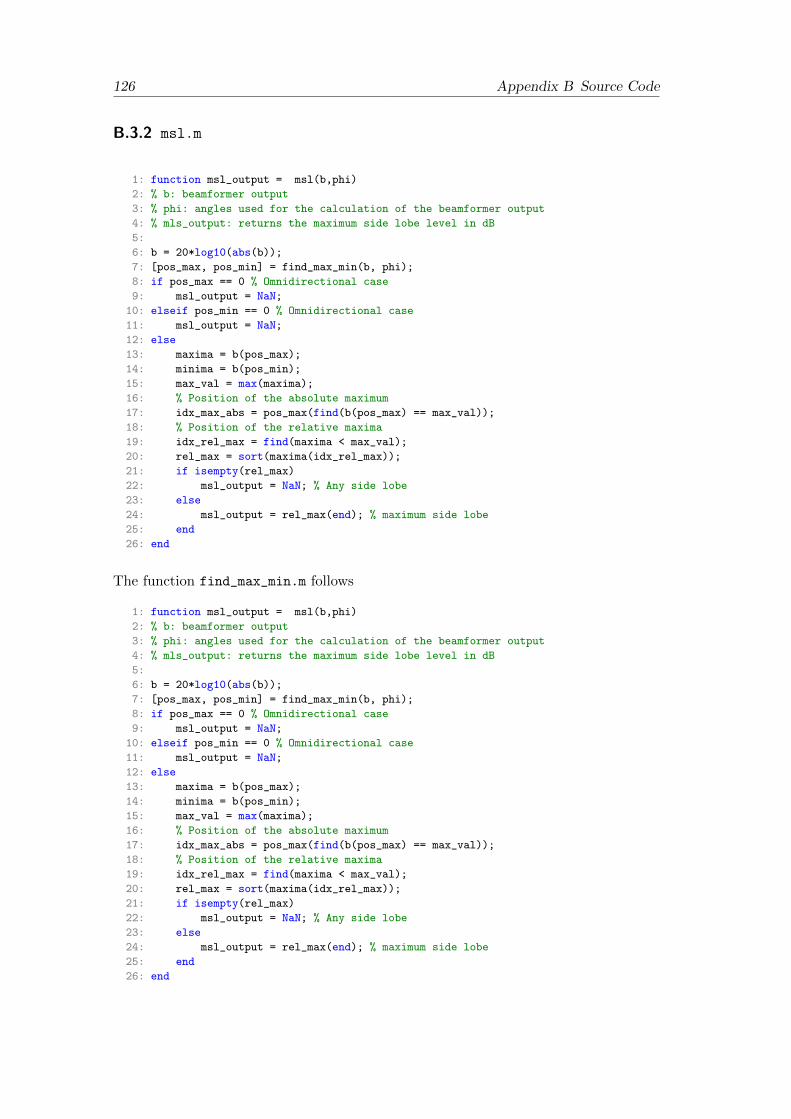
126 Appendix B Source Code
B.3.2 msl.m
1: function msl_output = msl(b,phi)
2: % b: beamformer output
3: % phi: angles used for the calculation of the beamformer output
4: % mls_output: returns the maximum side lobe level in dB
5:
6: b = 20*log10(abs(b));
7: [pos_max, pos_min] = find_max_min(b, phi);
8: if pos_max == 0 % Omnidirectional case
9: msl_output = NaN;
10: elseif pos_min == 0 % Omnidirectional case
11: msl_output = NaN;
12: else
13: maxima = b(pos_max);
14: minima = b(pos_min);
15: max_val = max(maxima);
16: % Position of the absolute maximum
17: idx_max_abs = pos_max(find(b(pos_max) == max_val));
18: % Position of the relative maxima
19: idx_rel_max = find(maxima < max_val);
20: rel_max = sort(maxima(idx_rel_max));
21: if isempty(rel_max)
22: msl_output = NaN; % Any side lobe
23: else
24: msl_output = rel_max(end); % maximum side lobe
25: end
26: end
The function find_max_min.m follows
1: function msl_output = msl(b,phi)
2: % b: beamformer output
3: % phi: angles used for the calculation of the beamformer output
4: % mls_output: returns the maximum side lobe level in dB
5:
6: b = 20*log10(abs(b));
7: [pos_max, pos_min] = find_max_min(b, phi);
8: if pos_max == 0 % Omnidirectional case
9: msl_output = NaN;
10: elseif pos_min == 0 % Omnidirectional case
11: msl_output = NaN;
12: else
13: maxima = b(pos_max);
14: minima = b(pos_min);
15: max_val = max(maxima);
16: % Position of the absolute maximum
17: idx_max_abs = pos_max(find(b(pos_max) == max_val));
18: % Position of the relative maxima
19: idx_rel_max = find(maxima < max_val);
20: rel_max = sort(maxima(idx_rel_max));
21: if isempty(rel_max)
22: msl_output = NaN; % Any side lobe
23: else
24: msl_output = rel_max(end); % maximum side lobe
25: end
26: end

B.4 Other Functions used for the Simulations 127
B.4 Other Functions used for the Simulations
B.4.1 plane_wave.m
1: function p = plane_wave(k,R,phi_s,phi_M,condition)
2: % k = wavenumber
3: % R = array radius
4: % phi_s = position of the source
5: % phi_M = position of the microphones
6: % condition = ’unbaffled’ or ’baffled’ for an array mounted on a cylindrical
rigid baffle of infinite length
7:
8: N = 60; % maximum order that avoids NaN in the range from 1 Hz to 3000 Hz
9: if strcmpi(condition,’unbaffled’)
10: p = (exp(-j*k*R*cos(phi_M-phi_s))).’;
11: elseif strcmpi(condition,’baffled’)
12: p = 0;
13: for n = -N:N
14: p = p + (-i)ˆn*(besselj(n,k*R)-besselj_prime(n,k,R).*hankel1(n,k*R)./
hankel1_prime(n,k,R))*exp(j*n*(phi_M-phi_s));
15: end
16: p = p.’;
17: end
B.4.2 random_noise.m
1: function n = random_noise(Ps,SNR)
2: % n = random_noise(Ps,SNR)
3: % Ps = Power signal
4: % SNR = SNR in dB
5: % random_val = randn(size(Ps)) + j*randn(size(Ps));
6: % n = (sqrt(Ps./(SNR*abs(random_val).ˆ2/2)).*random_val);
7:
8: SNR = 10ˆ(SNR/10);
9: abs_n = sqrt(2*Ps/SNR); % Noise magnitude
10: phase_n = 2*pi.*rand(size(Ps)); % Phase uniformly distributed from 0 to 2*pi
11: n = abs_n.*exp(j*phase_n); % Noise in complex notation


CFacility, Device and Software List
129

130
App
end
ixC
Facility,
Dev
icean
dSoftw
areL
ist
Table C.1: Used facilities, devices and software.
Type Manufacturer Model/name Description/notes
AnechoicChamber
Large anechoic roomin building 354(room 027) at DTU
Free space volume of about 1000 m3. Lower limiting fre-quency of about 50 Hz.
Circular Array Bruel & Kjær Prototype Circular array with a radius of 11.9 cm. It contains 12equispaced microphones, all of them being Bruel & Kjær1/4 ” microphones B&K Type 4935.
ControllableTurntable
Bruel & Kjær B&K Type 5960 Turntable capable to rotate with an accuracy of 1∘.
TurntableController
Bruel & Kjær B&K Type 5997 Remote controller for the turntable.
MultichannelPortablePULSE
Bruel & Kjær The front-end includes 5 sets of 12-channel Input ModuleB&K Type 3038 B, a Power-Supply Module B&K Type2826 and a 5/1-channel Input/Output Controller ModuleB&K Type 7539 A.
PortablePULSE
Bruel & Kjær The front-end includes a 4/2-channel Input/Output Mod-ule B&K Type 3109 and a LAN Interface Module B&KType 7533
Amplifiers Homemade amplifiers.
SphericalLoudspeaker
Loudspeaker unit mounted on a sphere.
Loudspeaker Dynaudio Acoustics BM 6A Two-way loudspeaker system.
Continued on the next page. . .

131
Table C.1: Used facilities, devices and software (continued).
Type Manufacturer Model/name Description/notes
Calibrator Bruel & Kjær B&K Type 4230 Produces 94 dB at 1 kHz. Used with an adapter for 1/4 ”microphones.
Sound LevelMeter
Bruel & Kjær B&K Type 2250 Hand-held sound level meter set with the template ‘Fre-quency Analyzer’ to measure environmental noise.
Software Bruel & Kjær Software for the PULSE system. The template ‘NS-STSFIrregular Array’ of the environment ‘Noise Source Iden-tification’ is used to acquire the data from the array.
Software Bruel & Kjær B&K BZ5503 Utility software for the sound level meter B&K Type2250.
Software The MathWorks Matlab Version7.6.0.324 (R2008a)
Among others including the Signal Processing Toolbox.
Computer Used for the software of the Multichannel PortablePULSE, and for Matlab.
Laptop Used for the software of the Portable PULSE.


Abbreviations and Symbols
Abbreviations
CHB Circular Harmonics beamforming
CH Circular harmonics
DSB Delay-and-Sum beamforming
DS Delay-and-Sum
MSL Maximum side lobe level
SNR Signal-to-noise ratio
Greek Symbols
' Azimuthal angle in the xy-plane
'i ' coordinate of the wavenumber vector ki
'm Angular position of the m’th microphone in a circular array
's Angular position of a source
! (Angular) Frequency [rad/s]
�0 Equilibrium density of the medium (≈ 1.204 kg/m3 for air at 20∘)
Roman Symbols
bN,CH Normalized output of a CH beamformer
bN,DS Normalized output of a DS beamformer
c Speed of sound (≈343 m/s for air at 20∘)
C�n Fourier coefficient of order n for a circular aperture mounted on a rigidcylindrical baffle of infinite length
C�n Fourier coefficient of order n for a circular array mounted on a rigid cylin-drical baffle of infinite length
CLn Fourier coefficient of order n for a circular aperture mounted on a rigidcylindrical baffle of length 2L
C∘n Fourier coefficient of order n for an unbaffled circular aperture
C∘n Fourier coefficient of order n for an unbaffled circular array
f Frequency [Hz]
133

134 Abbreviations and Symbols
H(1)n (x) Hankel function of first kind and order n with argument x
H(2)n (x) Hankel function of second kind and order n with argument x
H′n(kR) Derivative of Hn(kr) with respect to r, evaluated at r = R
j Imaginary unit, j2 = −1
Jn(x) Bessel function of order n with argument x
J′n(kR) Derivative of Jn(kr) with respect to r, evaluated at r = R
k Wavenumber
ki Wavenumber vector of an incident plane wave
L Half the length of a cylinder (2L).
M Number of microphones that conform an array
MSL Maximum side lobe level
N Maximum order used to decompose the sound field with circular harmonics
p Sound pressure in complex notation
R Radius of a cylinder, circular array or circular aperture
RES Resolution
SNRm Signal-to-Noise ratio at the input of each microphone of a circular array
Yn(x) Neumann function of order n with argument x

Bibliography
[1] Maynard, J., Williams, E. and Lee, Y., Nearfield Acoustic Holography: I.Theory of Generalized Holography and the Development of NAH, J. Acoust. Soc.Am., Vol. 4, No. 78, pp. 1397–1413, October 1985.
[2] Hald, J., Basic Theory and Properties of Statistically Optimized Near-field Acous-tical Holography, J. Acoust. Soc. Am., Vol. 4, No. 125, pp. 2105–2120, April 2000.
[3] Hald, J., Handbook of Signal Processing in Acoustics. Chapter 9., Springer NewYork, 2008.
[4] Johnson, D. and Dudgeon, D., Array Signal Processing Concepts and Tech-niques, Prentice Hall, 1993.
[5] Brandstein, M. and Ward, D., Microphone Arrays. Signal Processing Tech-niques and Applications, Springer, 2001.
[6] Meyer, J. and Elko, G., A Highly Scalable Spherical Microphone Array based onan Orthonormal Decomposition of the Soundfield, IEEE International Conferenceon Acoustics, Speech and Signal Processing (CASSP’02), Vol. 2, pp. 1781–1784,2002.
[7] Rafaely, B., Plane-wave Decomposition of the Sound Field on a Sphere by Spher-ical Convolution, J. Acoust. Soc. Am., Vol. 116, No. 4, pp. 2149–2157, October2004.
[8] Hald, J., Spherical Harmonics Beamforming, Bruel & Kjær internal paper.
[9] Teutsch, H. and Kellermann, W., Acoustic Source Detection and Localizationbased on Wavefield Decomposition using Circular Microphone Arrays, J. Acoust.Soc. Am., Vol. 120, No. 5, pp. 2724–2736, November 2006.
[10] Jacobsen, F., Propagation of Sound Waves in Ducts, Acoustic Technology, DTUElectrical Engineering, August 2006, lecture Note 31260.
[11] Pierce, A., Acoustics: An Introduction to its Physical Principles and Aplications,McGraw-Hill, 1981.
[12] Jacobsen, F. and Juhl, P., Radiation of sound, Acoustic Technology and In-stitute of Sensors, Signals and Electrotechnic, DTU Electrical Engineering andUniversity of Southern Denmark, April 2007.
[13] Morse, P. and Feshbach, H., Methods of Theoretical Physics, McGraw-Hill,1953.
135
136 Bibliography
[14] Morse, P. and Ingard, K., Theoretical Acoustics, McGraw-Hill, 1968.
[15] Teutsch, H., Modal Array Signal Processing: Principles and Applications ofAcoustic Wavefield Decomposition, Springer, 2007.
[16] Hartmann, W., Signals, Sound, and Sensation, Springer, 1997.
[17] Williams, E., Fourier Acoustics: Sound Radiation and Nearfield Acoustic Holog-raphy, Academic Press, 1999.
[18] Van Trees, H., Optimum Array Processing. Part IV of Detection, Estimation,and Modulation Theory, John Wiley & Sons, 2002.
[19] Elko, G. and Meyer, J., Springer Handbook of Speech Processing. Part I. 50,Springer, 2008.
[20] Jourdan, J. and Marschall, M., Comparison of Beamforming Techniques on aSphere, Tech. rep., Acoustic Technology – DTU Elektro, October 2008.
[21] Christensen, J. and Hald, J., Technical Review, Tech. rep., Bruel & Kjær, 2004.
[22] Spiegel, M., Liu, J. and Abellanas, L., Schaum. Formulas y Tablas deMatematica Aplicada, McGraw-Hill, 2005.
[23] Asmar, N., Partial Differential Equations, Prentice Hall, 2nd edn., 2000.
[24] Skudrzyk, E., The Foundations of Acoustics, Springer-Verlag/Wien, 1971.