noise source identification

techniques

Professor Phil Joseph

NOISE SOURCE LOCATION AND IDENTIFICATION

TECHNIQUES

Objectives

To locate and quantify the major sources of unwanted noise levels

Definitions

Noise: Unwanted sound

Source: Any physical mechanism that genets audio-frequency sound

Purposes:

i. To aid the choice of appropriate noise control measures

ii. To rank the importance of various noise control measures

iii. To identify the causes of the various sources

HOW MANY SOURCES ARE PRESENT?

Example:

The interior noise in a vehicle is due to the vibrating walls.

This vibration is due to other source mechanisms.

Which is the source and how many are there?

For example, is the vibrating wall a single ‘source’ or a number of sources

corresponding to a number of smaller sub-sources? What criteria do we

use to decide this?

MAJOR SOURCE LOCATION TECHNIQUES

Traditional Techniques

i. Human auditory system

ii. Partial Screening Techniques

iii. Directional Microphones

iv. Microphone Arrays

Modern Techniques

i. Sound Intensity Mapping

ii. Coherence Analysis

iii. Principal Component Analysis

iv. Inverse Techniques

v. Acoustical imaging/holography

1. HUMAN AUDITORY SYSTEM

The human hearing system is directional in terms of perceived loudness above

300Hz. The human hearing system detects the differences in times

between the signal arrival at the two ears. The effectiveness with which the

ear can localise sounds depends upon:

i. number and directional distribution of significant uncorrelated

noise sources. The fewer the better.

ii. relative strengths of direct and reverberant (reflected) sound.

Localisation ability reduces with increasing reverberation

(reflections).

iii. auto-correlation function of the signal (improves with decreasing

correlation length).

Nevertheless, the ear is remarkably good at localising a single broadband

source in very reverberant environments providing the direct sound is

received.

The hearing system is very poor at localising sources in the geometric near

field where there are many arrival directions, in small reverberant

environments (such as a car) or when there are many sources of the same

frequency in a reverberant room.

2. PARTIAL SCREENING TECHNIQUES Typically uses lead covering – still in common use

Example: In order to identify crankcase radiated noise on an engine

the remainder of the engine could be lead covered, and

the intake and exhaust pipes ducted away.

There are a number of problems with this approach

· Engine sources are likely to be correlated – the resulting spatial

interference pattern will change and the radiation impedance of

individual components can be altered. Ineffective at low

frequencies.

· Covering can change running temperature and conditions.

· A badly designed system for ducting away an exhaust could

change the back-pressure or engine running conditions, thus

changing intake and engine radiated noise.

3. DIRECTIONAL MICROPHONES

Sensitivity (voltage output per unit pressure) depends on plane

wave angle of arrival. Examples:

i. Cardioid Microphones

ii. Ribbon Microphones for measuring particle velocity

iii. Pressure difference Microphone

Directivity only useful at very high

frequencies. Main lobe generally

too broad to give acceptable

spatial resolution. Ambiguity

between strong off-axis sources

and weak on-axis sources.

END FIRE (or tube, or wave interference microphones)

Single tube with a series of holes along the length and a microphone

located at one end.

Pressure directivity D(q) given by

qqq cos1//cos1sin LLD

Advantages

i. Cheaper and simple to construct

ii. Good rejection of sound from the

rear

Disadvantages

i. Difficult to calibrate

ii. Tube length too long below 1kHz

iii. Very sensitive to flow (wind)

iv. Not effective in very reverberant

sound fields

ACOUSTIC MIRRORS Microphone located at the focus of parabolic ‘mirror’.

Advantages: - Simple and therefore

robust measurement principle - No

signal processing required.

Disadvantages: Large and heavy. It

has been estimates that a mirror

diameter of at least 8m is needed for

aero-engine source location. Aperture

must be much longer than acoustic

wavelength to be effective. Mirror

must be constructed very accurately.

Performance degrades in reverberant

environments due to off-axis sources

and diffraction effects by the large

mirror.

MICROPHONE ARRAYS PLANE WAVE BEAMFORMING

(also called delay and sum beamforming)

p lan e wav e fro n tq

d n

dsin

q

Let denote the pressure signal received at the nth

sensor as a function of time t due to an incoming

plane wave. The (un-shaded) beamformed output

b(t) by a linear array of uniformly spaced sensors is

given by f tn

b t f tn nn

N

1

q

nnd

c

sin

Taking the Fourier Transform of b(t) gives

B F in nn

N

exp1

F f t e dtn ni t

where

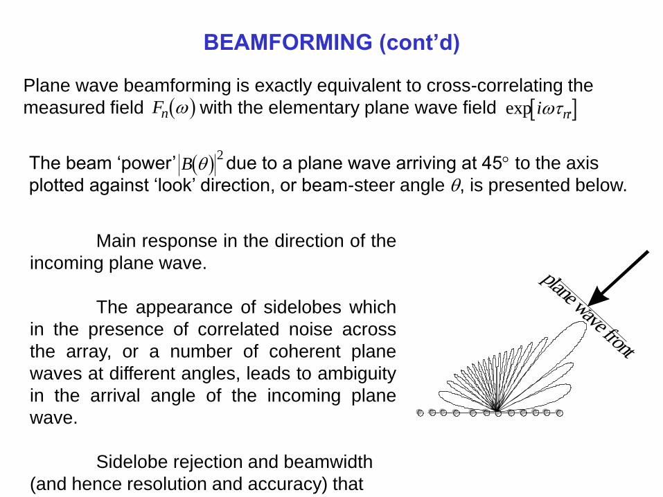
BEAMFORMING (cont’d)

Plane wave beamforming is exactly equivalent to cross-correlating the

measured field with the elementary plane wave field . Fn exp i n

The beam ‘power’ due to a plane wave arriving at 45 to the axis

plotted against ‘look’ direction, or beam-steer angle q, is presented below. B q

2

plane wave front

Main response in the direction of the

incoming plane wave.

The appearance of sidelobes which

in the presence of correlated noise across

the array, or a number of coherent plane

waves at different angles, leads to ambiguity

in the arrival angle of the incoming plane

wave.

Sidelobe rejection and beamwidth

(and hence resolution and accuracy) that

improve with increasing number of sensors.

PLANAR ARRAYS FOR SOURCE LOCATION IN

TWO DIMENSIONS

Same principle applied. For an arbitrary array of sensors with position

vectors r, the beam power output of the array in the direction of u is given by

B E H H H Hu w p w p w Rw

2

where and R is the spatial covariance matrix w a ei ij k i r u. R E p pij i j r r

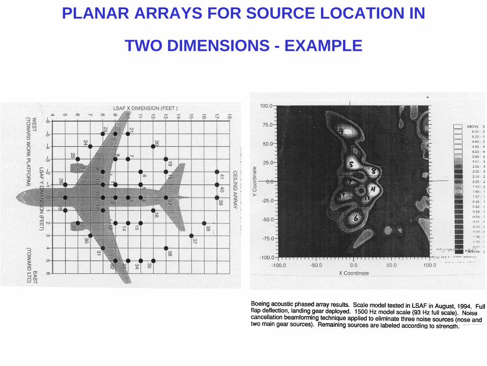
PLANAR ARRAYS FOR SOURCE LOCATION IN

TWO DIMENSIONS - EXAMPLE

SOUND INTENSITY FOR SOURCE LOCATION Time-stationary sound intensity vectors (3-D) are measured with intensity

probes (see intensity lecture). Intensity contours showing the magnitude

and direction of energy flow may be used to reveal the location and

magnitude of the various noise sources. There are two principal modes of

operation. i. Reverse Vector Projection

Determine intensity vector distribution in

geometric near field and project back

energy flow contours to the source surface.

Intensity is the vector sum of intensities

due to uncorrelated sources. It cannot

therefore resolve such sources. Intensity

techniques for source location is useful

when there is only one dominant source.

Narrow band, or tonal, intensity

distributions in reverberant environments

are very complicated. It can be difficult to

project back to the source region.

Broadband sources are more reliable.

ii. Near field rank ordering

Estimate sound power radiated by

segments of the source surface by

near field scans. Rank order the

‘sources’ on this basis. Technique is

effective for efficient radiators. Caution

should be exercised - not all local

near field power propagates to the far

field.

MODERN TECHNIQUES

Since the advent of the fast and inexpensive processing capabilities

available on modern desktop computers new techniques have recently

been proposed for source indication.

In this lecture we shall only briefly mention three and give details of a

fourth.

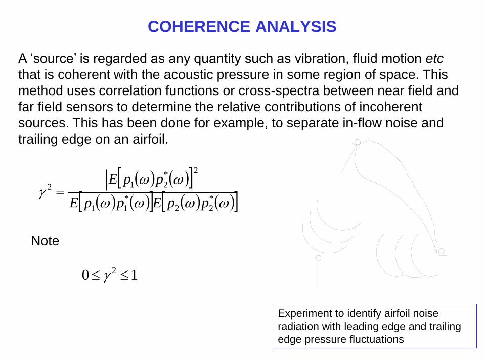
COHERENCE ANALYSIS

A ‘source’ is regarded as any quantity such as vibration, fluid motion etc

that is coherent with the acoustic pressure in some region of space. This

method uses correlation functions or cross-spectra between near field and

far field sensors to determine the relative contributions of incoherent

sources. This has been done for example, to separate in-flow noise and

trailing edge on an airfoil.

*

22

*

11

2*

212

ppEppE

ppE

10 2

Note

Experiment to identify airfoil noise

radiation with leading edge and trailing

edge pressure fluctuations

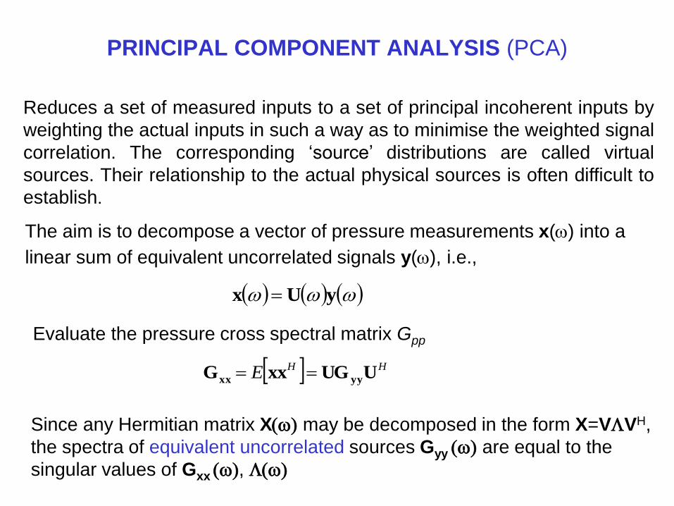
PRINCIPAL COMPONENT ANALYSIS (PCA)

Reduces a set of measured inputs to a set of principal incoherent inputs by

weighting the actual inputs in such a way as to minimise the weighted signal

correlation. The corresponding ‘source’ distributions are called virtual

sources. Their relationship to the actual physical sources is often difficult to

establish.

The aim is to decompose a vector of pressure measurements x() into a

linear sum of equivalent uncorrelated signals y(), i.e.,

Evaluate the pressure cross spectral matrix Gpp

yUx

HHE UUGxxG yyxx

Since any Hermitian matrix X may be decomposed in the form X=VLVH,

the spectra of equivalent uncorrelated sources Gyy are equal to the

singular values of Gxx , L

SOURCE POWER BREAKDOWN FROM VELOCITY

MEASUREMENTS

1. The mean square velocity is measured over a vibrating structure.

2. The structure is then suitably divided into a number of simple sub-

structures that resemble simple vibrating elements, such as flat plate.

3. Together with an estimate for the radiation efficiency, this information is

used to assess the individual component sound power contributions to

total radiated sound power.

NEAR FIELD ACOUSTICAL HOLOGRAPHY (NAH)

A technique for reconstructing the source by taking the wavenumbers

transforms of the acoustic pressure made close by. The technique is

fundamentally dependent upon the following Fourier relationships:

Wavenumber spectrum of pressure related to spatial variation by

dxezxpzkpxjk

11 ),(),(

Wavenumber spectrum of surface velocity related to spatial

variation by

dxexukuxjk

11 )()(

Measurable pressure wavenumber spectrum and surface velocity (source)

wavenumber spectrum related by

)(

)(),(

21

2

)21

2(

101

kk

ekuzkp

zkkj

Note that wavenumber

components propagate for

and decay for kk || 1

kk || 1

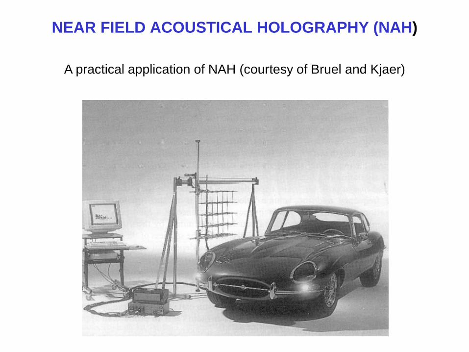
A practical application of NAH (courtesy of Bruel and Kjaer)

NEAR FIELD ACOUSTICAL HOLOGRAPHY (NAH)

INVERSE PROBLEMS

DISCRETISATION OF THE FORWARD PROBLEM

Assume a model of the

form

p = G q

NMNMM

N

N

M q

q

q

GGG

GGG

GGG

p

p

p

.

.

.

..

.

.

...

...

.

.

.

2

1

21

22221

11111

2

1

which can be written in full as

INVERSE PROBLEMS (cont’d)

Least Squares Solution

Find the discrete source strengths that “best fit” the measured pressures.

Assume:

eGqp ˆ

Need to find optimal q that minimises

M

mmm ppJ

1

2H ˆee

For M > N, this quadratic function of q is minimised by

pGGGq ˆ][ H1H0

Or when M = N

pGq ˆ10

Note that solution is unique for the assumed source model

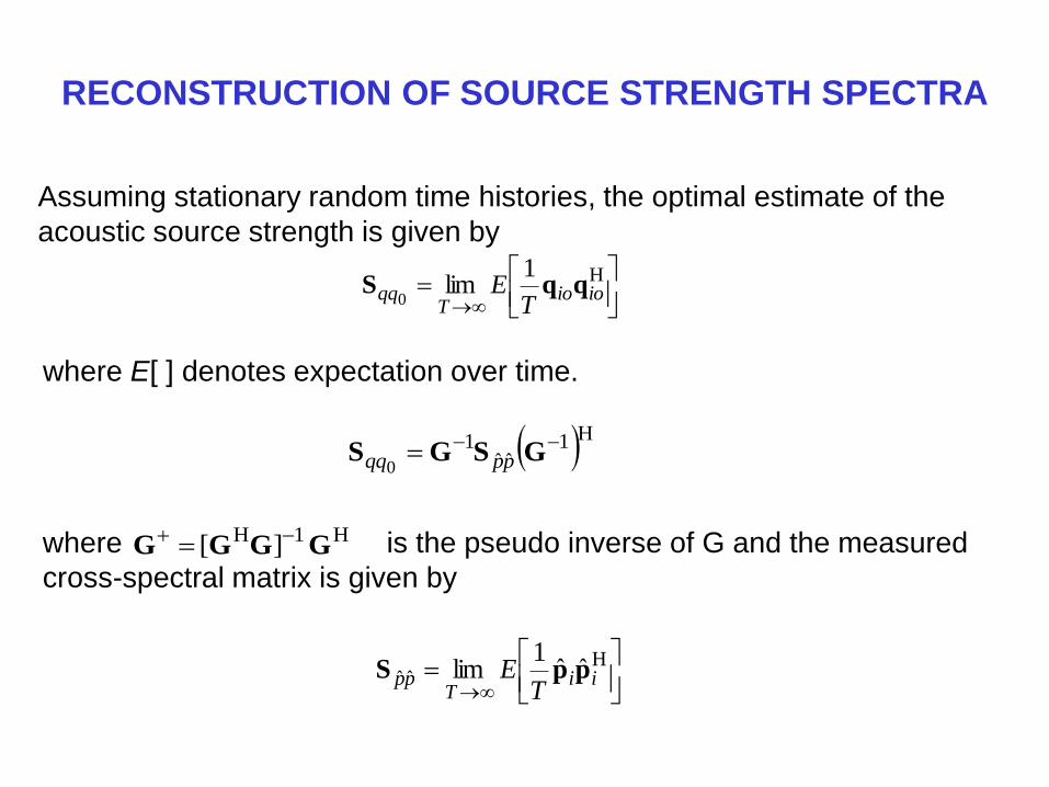
RECONSTRUCTION OF SOURCE STRENGTH SPECTRA

H1lim

0 ioioT

qqT

E qqS

H1H ][ GGGG

Hˆˆ ˆˆ

1lim ii

Tpp

TE ppS

H1ˆˆ

1

0

GSGS ppqq

Assuming stationary random time histories, the optimal estimate of the

acoustic source strength is given by

where E[ ] denotes expectation over time.

where is the pseudo inverse of G and the measured

cross-spectral matrix is given by

EXPERIMENTAL EXAMPLE

(S. H. Yoon, PhD thesis, University of Southampton 1998)

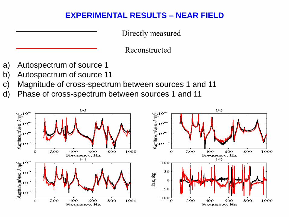
EXPERIMENTAL RESULTS – NEAR FIELD

Directly measured

Reconstructed

a) Autospectrum of source 1

b) Autospectrum of source 11

c) Magnitude of cross-spectrum between sources 1 and 11

d) Phase of cross-spectrum between sources 1 and 11

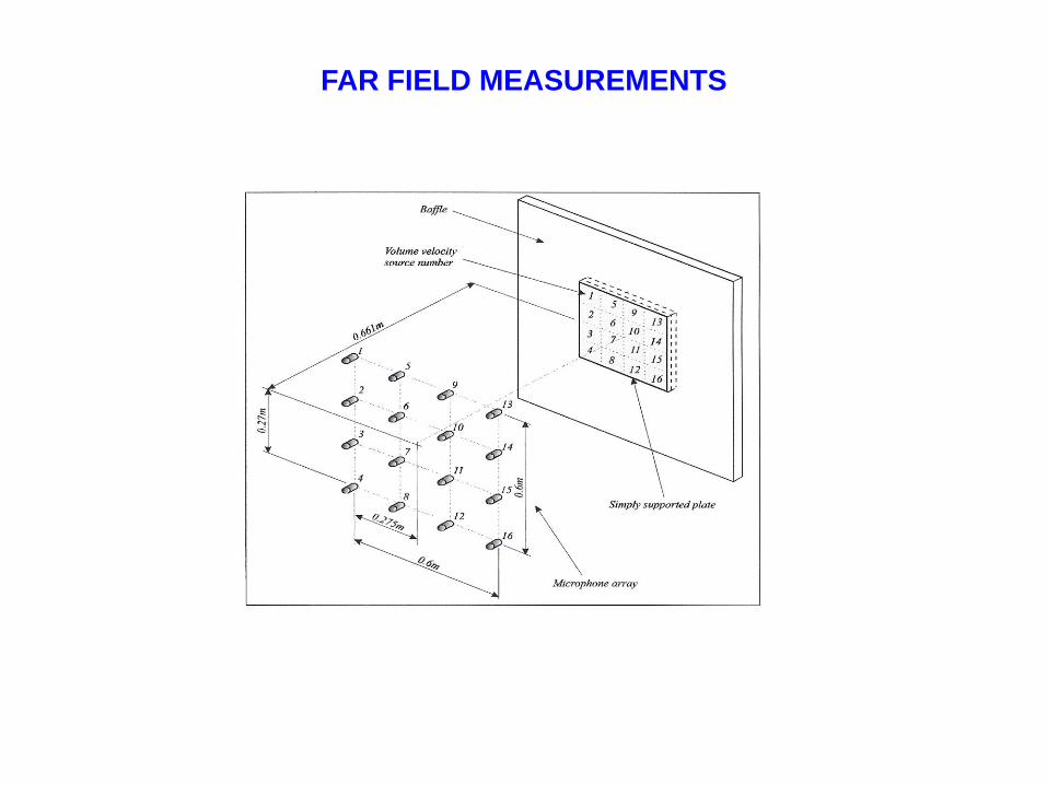
FAR FIELD MEASUREMENTS

EXPERIMENTAL RESULTS – FAR FIELD

Directly measured

Reconstructed

a) Autospectrum of source 1

b) Autospectrum of source 11

c) Magnitude of cross-spectrum between sources 1 and 11

d) Phase of cross-spectrum between sources 1 and 11

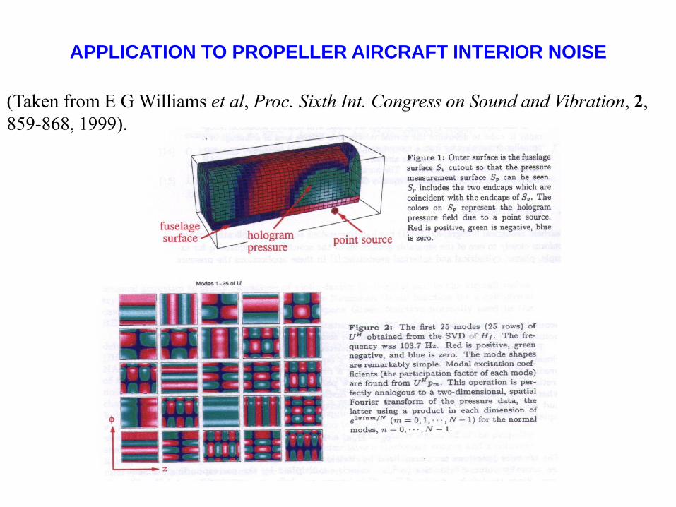
APPLICATION TO PROPELLER AIRCRAFT INTERIOR NOISE

(Taken from E G Williams et al, Proc. Sixth Int. Congress on Sound and Vibration, 2,

859-868, 1999).

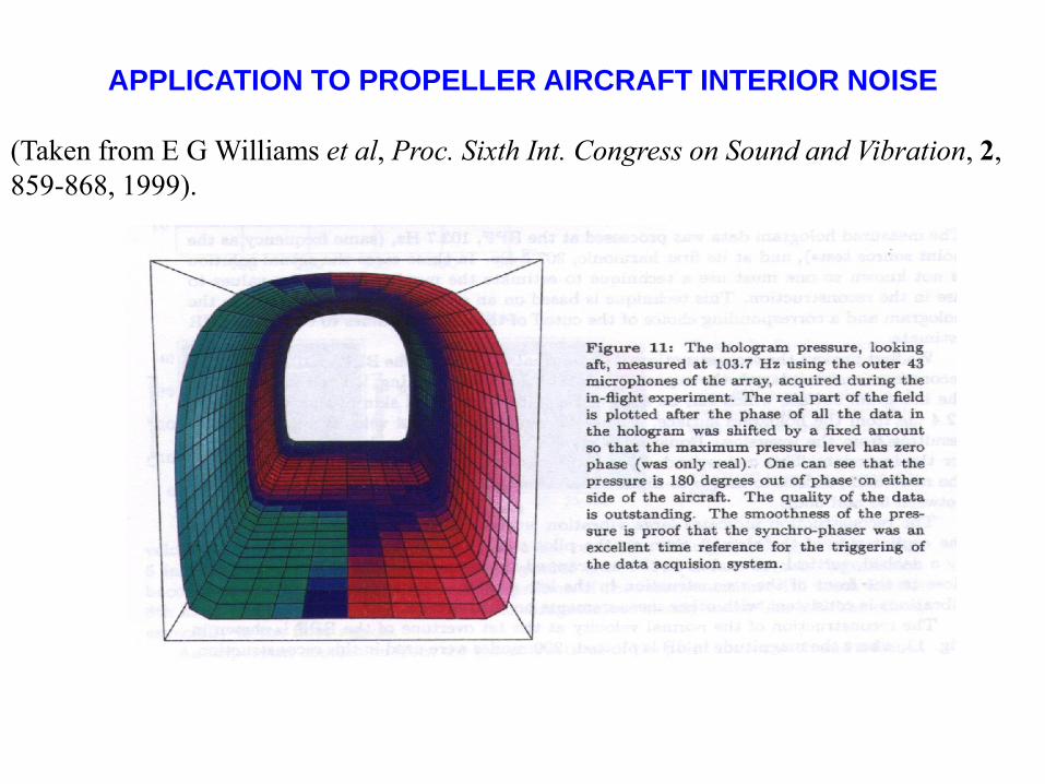
APPLICATION TO PROPELLER AIRCRAFT INTERIOR NOISE

(Taken from E G Williams et al, Proc. Sixth Int. Congress on Sound and Vibration, 2,

859-868, 1999).

APPLICATION TO PROPELLER AIRCRAFT INTERIOR NOISE

(Taken from E G Williams et al, Proc. Sixth Int. Congress on Sound and Vibration, 2,

859-868, 1999).

APPLICATION TO PROPELLER AIRCRAFT INTERIOR NOISE

(Taken from E G Williams et al, Proc. Sixth Int. Congress on Sound and Vibration, 2,

859-868, 1999).