silhouette

150 IEEE TRANSACTIONS ON PATTERN ANALYSIS AND MACHINE INTELLIGENCE, VOL. 16, NO. 2, FEBRUARY 1994

The Visual Hull Concept for Silhouette-Based Imaee Understanding U U

Aldo Laurentini

Abstract- Many algorithms for both identifying and reconstructing a 3-D object are based on the 2-D silhouettes of the object. In general, identifying a nonconvex object using a silhouette- based approach implies neglecting some features of its surface as identification clues. The same features cannot be reconstructed by volume intersection techniques using multiple silhouettes of the object.

This paper addresses the problem of finding which parts of a nonconvex object are relevant for silhouette-based image understanding. For this purpose, the geometric concept of visual hull of a 3-D object is introduced. The visual hull of a 3-D object S is the closest approximation of S that can be obtained with the volume intersection approach. An equivalent statement, relative to object identification, is that the visual hull of S is the maximal object silhouette-equivalent to S, i.e., which can be substituted for S without affecting any silhouette. Only the parts of the surface of S that also lie on the surface of the visual hull can be reconstructed or identified using silhouette-based algorithms. The visual hull of an object depends not only on the object itself but also on the region allowed to the viewpoint. Two main viewing regions can be considered, resulting in the external and internal visual hull. In the former case the viewing region is related to the convex hull of S, in the latter it is bounded by S itself. The internal visual hull also admits an interpretation not related to silhouettes: the features of the surface of S that is not coincident with the surface of the internal visual hull cannot be observed from any viewpoint lying outside the convex hull.

After a general discussion of the visual hull and its properties, algorithms for computing the internal and external visual hulls of 2-D objects and 3-D planar face objects are presented and their complexity analyzed. In general, the visual hull of a 3-D planar face object turns out to be bounded by planar and curved patches. A precise statement of the concept of visual hull appears to be novel, as is the problem of its computation.

Index Terms- Computer vision, image understanding, shape recognition, silhouettes, shape from contour, volume intersection, convex hull, visual hull.

I. INTRODUCTION

0 understand the 3-D content of a scene is a central T problem in computer vision, since it can allow computer- driven equipment to perform tasks such as navigation, ma- nipulation, and visual recognition. Many approaches have been proposed for identifying or reconstructing 3-D objects when 2-D images are available; these approaches are usually categorized as shape-from-X, according to the information used.

Manuscript received March 2, 1992; revised October 2, 1992. Recom- mended for acceptance by Associate Editor T. Henderson.

The author is with the Dipartimento di Automatica ed Informatica, Politec- nico di Torino, 10129 Turin, Italy.

IEEE Log Number 9212303.

0 162-8828/94$04

V

Fig. 1. The volume intersection approach to object reconstruction.

Among other image cues, the silhouettes of a 3-D object S can be selected as sources of shape information. The 2-D silhouette, obtained as a parallel or perspective projection of S onto the image plane, has been indicated as an effective psychophysical clue to shape understanding [ 13. Object recognition based on silhouettes has been performed for many years by human observers. Referring to computer- based systems, obtaining the 2-D silhouette is usually a computationally simple task, one that can be most often performed by thresholding an intensity image. The algorithms for obtaining the silhouettes, or their boundaries, usually also perform well with degraded images. For these reasons, the silhouette is a favorite cue for image understanding.

A number of silhouette-based algorithms have been proposed for object identification [2]-[9]; many industrial vision systems also identify objects or their attitude using silhouettes.

Object reconstruction can be performed using the volume intersection approach, which recovers the volumetric description of the object from multiple silhouettes. This approach, proposed in [lo] by Martin and Aggarwal, and used by many object reconstruction algorithms [I I]-[ 171, consists in intersecting the solid regions of space in which the object is constrained to lie by each silhouette. These regions are cones obtained by back projecting from a viewpoint V the corresponding silhouette for perspective projections (see Fig. I), or cylinders obtained by sweeping the silhouette along a line parallel to the viewing direction for orthographic projections. In the following, as the orthographic projection can be considered a limit case of perspective projection, we will always refer to these regions as cones. The boundary of each cone, which consists of all the half-lines starting at V and tangent to S, will be referred to as the circumscribed cone of S relative to V.

As the number of cones increases, the object is reconstructed with higher precision. Some papers also address the problem

.OO 0 1994 IEEE

LAURENTINI: THE VISUAL HULL CONCEPT 151

Fig. 2. Two objects that cannot be distinguished using silhouettes Fig. 3. Two objects that cannot be reconstructed using volume intersection.

of specifying the viewpoints that optimize the construction, without a priori information on the object [ 181.

In spite of their attractive features, silhouettes can be insufficient clues for fully understanding 3-D shapes. It is clear that identification algorithms based on silhouettes are not always able to discriminate different nonconvex objects. For instance, no silhouette-based algorithm appears to be able to tell one of the two objects SI and S2 in Fig. 2 from the other. The difference between SI and S2 consists in a small cube that lies in a concavity. It is easy to understand that this cube does not manifest itself in any possible silhouette of the objects, at least considering viewpoints not too near to the object.

The silhouette-based approach to object identification therefore raises questions like the following.

Which part of the surface of a 3-D object S can affect the silhouettes of the object? To what extent can the complementary part of the surface of S take different shapes without affecting any silhouette?

The algorithms based on the volume intersection approach are not able to exactly reconstruct any possible object, not even performing infinite intersections. Here and in the following, “to exactly reconstruct” means “to reconstruct with arbitrarily high precision,” which is the correct statement referring to the reconstruction of general solids, e.g. a sphere. It is not difficult to recognize that none of the simple polyhedral objects SI and S2 in Fig. 2, and S, and S, in Fig. 3, can be exactly reconstructed using volume intersection, at least considering viewpoints not “too near” the object.

The silhouette-based approach to object reconstruction raises therefore questions such as the following.

Which part of the surface of a 3-D S object can be exactly reconstructed with volume intersection? When S cannot be exactly reconstructed, which is the closest approximation of S that can be obtained using volume intersection techniques?

Precise answers to all the previous questions will be pro- vided in the following sections. Here we will acquire some insight into the problem by inspecting the planar face object S4 in Fig. 3. This object is sufficiently simple to answer the previous questions by an intuitive analysis.

Let us assume that the possible viewpoints are not too near the object (we will specify in the following the precise meaning of this statement). It is not difficult to realize that the surface highlighted in Fig. 4(a) can be reconstructed by volume intersection. This is also the surface relevant for the silhouettes

0 silhouette-inactive surface

(a) (b)

Fig. 4. The behavior of Sq with respect to silhouette-based identification and reconstruction. (a) The silhouette-active and inactive surfaces of &. (b)S4 can assume any shape inside P without affecting any silhouette. ( c ) The closest approximation of Sq that can be obtained with volume intersection.

of S,. Let this surface be the silhouette-active surface of S4.

The complementary silhouette-inactive surface of S, is also shown in Fig. 4(a). This surface can take any shape, without affecting any silhouette, inside the pentahedron P shown in Fig. 4(b), bounded by the contour-inactive surface and the rectangle ABCD. The closest approximation of S4, i.e., the smallest object that can be obtained using volume intersection techniques, is the object in Fig. 4(c), which is the union of S4 and the pentahedron P.

The limits of the contour-based approach for understanding nonconvex shapes have been qualitatively recognized in many papers (see for instance [lo] and [l 11). Until now, however, to the author’s knowledge this topic has not been thoroughly discussed, and no general ’ answers to the previously stated questions are available.

The purpose of this paper is to develop a general geometric tool for dealing in a simple and straightforward way with the questions raised for nonconvex objects by the silhouette-based approach to image understanding. This tool will be called the visual hull of an object S. Referring the reader to the following section for more precise definitions, here we introduce the general idea of visual hull. Broadly speaking, the visual hull of an object S is the envelope of all the possible circumscribed cones of S . An equivalent intuition is that the visual hull is the maximal object that gives the same silhouette of S from any possible viewpoint. For instance, the visual hull of the sample object S4 is shown in Fig. 4(c). Its surface consists of two parts: the contour-active surface of S,, and the rectangle ABCD. We can consider this second surface as produced by all the visual rays tangent to S at the segments AB and atCD.

The visual hull idea has been first introduced by the author in [19], together with a preliminary algorithm for its compu-

I52 IEEE TRANSACTIONS ON PATTERN ANALYSIS AND MACHINE INTELLIGENCE. VOL. 16. NO. 2. FEBRUARY 1994

tation in 2-D. An algorithm for computing the visual hull of a solid of revolution is described in [20].

The content of this paper is as follows. In Section 11, precise definitions of visual hull are stated and its general properties analyzed. With reference to the possible regions that contain the viewpoints, two main cases are considered and the external and internal visual hulls are defined. In Section 111, efficient algorithms for computing both the internal and extemal visual hulls in 2-D are described. An algorithm for the computation of the silhouette-active surface of a 3-D polyhedral object, based on the 2-D algorithm of Section 111, is presented in Section IV. In Section V , the problem of computing the visual hull of a general polyhedron is addressed. The surfaces that are potential boundaries of the external and internal visual hulls of polyhedral objects are determined. It tums out that the visual hulls of polyhedra are bounded by planar and quadric surfaces. Finally, algorithms are presented for finding both visual hulls.

11. THE VISUAL HULL: DEFINITIONS AND GENERAL PROPERTIES

This section is organized as follows. In Section 11-A a formal definition of the visual hull of S relative to a viewing region is given. It is shown that this definition conforms to the intuitive discussion of Section I, and the questions there presented admit simple answers in terms of visual hull. In Section 11-B, considering viewpoints outside the convex hull of the object, we show that there is a unique visual hull, not exceeding the convex hull, for any viewing region completely enclosing S . We refer to this main case as the extemal visual hull. Section 11-C deals with an unrestricted viewing region. The corresponding intemal visual hull also supplies information on the part of surface of S that is not observable from points outside its convex hull.

A. The Visual Hull of an Object Relative to a Viewing Region

Let R be the viewing region of 3-D Euclidean space that contains the viewpoints that are allowed for observing the object S . We must take into account the position allowed to the viewpoint V , and we define the visual hull as dependent not only on S but also on R. We give the following simple geometric definition, which characterizes the points belonging to the visual hull.

Definition I: The visual hull V H ( S , R ) of an object S relative to a viewing region R is a region of E3 such that, for each point P E V H ( S , R ) and each viewpoint V E R, the half-line starting at V and passing through P contains at least a point of S.

We see obviously that S 5 V H ( S ) , since any point of S satisfies this definition. It is immediately possible to verify that Definition 1 satisfies the intuitive idea of visual hull stated in the introduction. In fact, the two following propositions can be obtained.

Proposition 1: V H ( S , R) is the maximal object silhouette- equivalent to S with respect to R (Le., that gives the same silhouette as S when observed from any V E R).

In fact, the following statements apply. 1 ) V H ( S, R ) is silhouette-equivalent to S with respect to

R, since 1) according to Definition 1 , the projection of any point P E V H ( S , X ) from any viewpoint V E R belongs to the silhouette of S obtained from V , and 2) the projection of any point Q E S from any viewpoint V E R belongs to the silhouette of V H ( S , R ) obtained from V , since S 5 V H ( S . R ) .

2 ) V H ( S. R) is the maximal silhouette-equivalent object, since for any point P’ $! V H ( S , R) , there is at least a line, starting at a point V’ E’ R and passing through P‘, that does not intersect S . Therefore the projection of P’ does not belong to the silhouette of S obtained from V’. This implies that P’ cannot belong to an object

Proposition 2 : V H ( S , R ) is the closest approximation of S that can be obtained using volume intersection techniques with viewpoints V E R.

In fact, only points P $! V H ( S , R ) can be removed by intersecting 3-D cones, since only such points can lie outside some silhouette and therefore outside some 3-D cone. 0

Another property of the visual hull can be readily obtained. Proposition 3: If R > R’, then V H ( S , R ) 5 V H ( S , RI). Of course, if a wider viewing region is available, a greater

number of cones can be intersected and more points can be removed. 0

In conclusion, the definition given for the visual hull of an object S relative to a viewing region R conforms to the intuitions reported in the introduction. The following answers to the questions there reported can be given in terms of visual hull:

silhouette-equivalent to S. U

sa(S, R) , the silhouette-active surface of S relative to the region R, is the part of the surface s ( S ) of S that also belongs to vh(S , R) , the boundary of V H ( S , R). si(S, R ) , the silhouette-inactive surface of S, can assume any shape inside the volume V H ( S , R ) - S without affecting any silhouette obtained from R. sa(S, R) is the part of s(S) that can be exactly reconstructed by volume intersection using silhouettes obtained from R. V H ( S . R) is the closest approximation of S that can be obtained by volume intersection using silhouettes obtained from R. Using the visual hull concept, other synthetic statements referring to silhouette-based image understanding can be formulated. For instance, the following rules apply. Two objects 5’ and S’ can be discriminated using their silhouettes observed from a viewing region R iff V H ( S , R) # VH(S’ , R). An object S can be exactly reconstructed by volume intersection techniques using silhouettes observed from a viewing region R iff S = V H ( S , R ) .

Let us make a final remark: Proposition 4: The silhouette-active surface m(S, R) of an

This proposition follows immediately from the fact that all object uniquely determines its visual hull V H ( S , R).


Fig. 5 . The visual hull relative 10 region.; completely enclosing .S helongs to its convex hull.

the circumscribed cones relative to an object are determined 0 uniquely by its silhouette-active surface.

B . The Main Case: The Exterml Visual Hull

According to definition I , there is an infinite set of visual hulls of an object S, one for each possible viewing region R. This seems to reduce in some way the effectiveness of the idea. Actually, we will show that for each object S there is a main case of visual hull, to which the majority of practical cases can be referred. In addition, we will see that this main case is related to C H ( S ) , the convex hull of S .

Observe first that in many practical cases I ) the object to be identified or reconstructed can assume any attitude with respect to the viewpoint V, and 2) V lies at some distance from the unknown object.

Let us consider therefore the visual hull VH(S . R’) relative to a region R’ that c~ompletdy enc~lo.ses S. Let us also suppose that

R’ E R,, = E” - C H ( S )

i.e.. no viewpoint is allowed inside the convex hull of the object. It is easy to show that the following proposition holds.

Proposition 5:

V H ( S . R’) 5 C H ( S ) .

To prove this statement, let us consider a point P C H ( S ) . We can easily find viewpoints such that the viewline passing through I’ does not intersect S. Viewpoints of this kind lie on the plane p passing through P and normal to the segment PC), where C ) is the point of C H ( S ) closest to P. In fact, by contradiction, let us suppose that the viewline VP, lying on p . intersects C,’H(S) at point T (see Fig. 5). Point R, which belongs to the convex hull as a linear combination of C) and T, and such that P R is normal to C)?‘. would be closer to P

0 Let us now consider another viewing region R”, which like

Pi-oposition 6 :

than (2, against the hypothesis.

R’ encloses S and lies outside the convex hull. We have

V H ( s, R’) = 17H( s. R”).

In fact, for any point C) E V H ( S . R’) , and for any half-line passing through C) and starting at I;.’ E R’, i t is possible to find a point ti” E R” on the same half-line. Vice-versa, for any point C ) E l ’H(S . 12’’) and for any half-line passing through (2 starting at V” E R”. it is possible to find a point b7’ E R’ on the same half-line (see Fig. 6). Therefore, according to definition I , any point C) belonging to L’H( S. R’) also belongs

0 to V H ( S. R”) and vice-versa.

Fig. 6. All the visual hulls of S relative to regions completely enclosing .S are equal.

I I

Fig. 7. The visual hulls relative to Ii”’ and R‘ are different.

Observe that proposition 6 is no more guaranteed to hold if one or both viewing regions have parts inside the convex hull, since one of these regions can have points inside the visual hull of the other. As an example, let us consider the 2-D case of Fig. 7, where the region R” has a part inside the convex hull of S . It can be easily verified by inspection that V H ( S. R’) contains the quadrangular region ABCD, and V H ( S . R”) contains the pentagonal region ABCDE. This is because the viewpoints of R” that also belong to V H ( S . R’) “dig” the visual hull relative to R‘, deleting the triangular region ADE.

In conclusion, there is a unique visual hull, not exceeding the convex hull of S , relative to all the viewing regions that enclose S and do not enter its convex hull.

Definition 2: V H ( S . R,) is defined as the e.rternal visual hull, or simply the visual hull of S, V H ( S ) , without any other specification.

The surface of S coincident with the surface nh.(S) of I’H(S) will be said to be the external silhouette-active surface of S or, briefly, the silhouette-active surface sa( S ) . Actually, according to the above discussion, the viewing region relatiive to the Isisual hull can estend also inside the convex hull, as long as it does not enter the visual hull itsev. This suggests another definition of external (or natural) visual hull: V H ( S ) is the largest visual hull of S whose viewing region is bounded by the visual hull itself.

V H ( S ) , which we made implicit reference to in the introduction considering viewpoints “not too near” to the object, has other interesting properties. Let us consider any viewing region R, that is a subset of R, and does not include S. The visual hull V H ( S . R,) relative to this region is strictly related to I’H(S). In fact, V H ( S . X , 9 ) contains V H ( S ) , and its surface ~rh(S. R,*) is equal to the surface v h ( S ) of V H ( S )

154 IEEE TRANSACTIONS ON PATTERN ANALYSIS AND MACHINE INTELLIGENCE, VOL. 16, NO. 2, FEBRUARY I994

Fig. 8. The visual hull relative to R, can be obtained from the visual hull relative to R, .

at the points of tangency to V H ( S ) of lines passing through R,. The remaining part of vh(S , R,) is bounded by the lines tangent to both R, and V H ( S ) , as it is shown by the example of Fig. 8, where 2-D sections of R,, V H ( S ) and V H ( S , R,) are presented.

A point Q E V H ( S ) can be characterized very simply in terms of lines passing through Q. In fact, we have the following proposition.

Proposition 7: Q belongs to V H ( S ) iff any line passing through P contains at least one point of S .

This statement will be used in the following for computing the visual hull.

C . The Internal Visual Hull

If the boundary of the viewing region is s itself, we have another case worth considering. Let Ri = E3 - S .

Definition 3 V H ( S , R,) is defined as the internal visual hull of S, I V H ( S ) .

The surface of S coincident with the surface ivh(S) of W H ( S ) will be said to be the internal silhouette-active surface of S , zsa(S). Also, let the complementary surface be the internal silhouette-inactive surface, isa (S).

The points belonging to the intemal visual hull can be simply characterized in terms of half-lines:

Proposition 8: Q belongs to I V H ( S ) . iff any half-line passing through Q contains at least one point of S.

This statement, like the previous one relative to the visual hull, will be used for constructing the internal visual hull.

An inspection of all the sample objects so far considered shows that their intemal visual hulls are equal to the corresponding objects.

It is not likely that an attempt will be made to recognize or reconstruct objects using silhouettes from a viewpoint lying inside their convex hull. However, the intemal visual hull admits another interesting visual interpretation not related to silhouettes. In fact, from proposition 8 the following follows immediately.

Proposition 9: i s i (S) , the intemal silhouette-inactive surface, cannot be observed from any viewpoint V $ C H ( S ) .

Therefore, the geometric concept of internal visual hull can be used for determining which features (edges, textures, etc.) of a 3-D nonconvex object will never appear on any image

of the object obtained from points outside the convex hull. Observe that to be V outside C H ( S ) is a sufficient condition for proposition 9 to hold; i s i (S) could be unobservable also from points belonging to C H ( S ) .

Since the viewing region relative to I V H ( S ) is the largest among the possible viewing regions, from proposition 3 we obtain the following.

Proposition 10:

I V H ( S ) 5 V H ( S ) .

111. THE COMPUTATION OF V H ( S ) AND OF I V H ( S ) IN 2-D

An effective use of the visual hull idea requires algorithms for its computation. The visual hull is basically a 3-D entity; algorithms for finding visual hulls in 2-D could appear of little use. Actually, the 2-D algorithms are able to deal with 2.5-D sweep solids. In addition, the 2-D algorithms and concepts are useful for solving the 3-D problem for planar face objects, as we will see in the following. Also, the algorithms for computing both visual hulls of solids of revolution presented in [20] stems from the 2-D algorithms.

The content of this section is as follows. In 111-A an algorithm for computing the visual hull of a set of polygons S P is presented. The algorithm is based on the simple observation that a point does not belong to the visual hull if there are lines passing through this point that do not intersect SP. It will be shown that these visual lines can be arranged into families, and the plane can be divided into polygonal zones such that the visual lines passing through every point of each zone can be arranged into the same number of families. After constructing this partition of the plane, the visual hull can be obtained visiting all the zones and merging the zones having zero families of visual lines.

In 111-B we present an algorithm for computing the internal visual hull. This algorithm is derived from the previous one, with suitable modifications.

A. An Efficient Algorithm for Computing the 2 - 0 Visual Hull

Let us consider a set of polygons S P in a plane p . To consider a nonconnected set of polygons is clearly a necessary condition for obtaining V H ( S P ) # C H ( S P ) . Let us define a visual line as a straight line belonging to p that does not intersect SP. The visual lines passing through a point Q can be grouped into a number of families, like those shown in Fig. 9.

Definition 4 : The visual number V N ( Q , S P ) of a point Q relative to S P is defined as the number of families of visual lines passing through Q.

It is clear that V N ( Q , S P ) cannot exceed the number of nonconnected components of SP. Referring to proposition 7, we have the following.

Proposition 11: A point Q belongs to V H ( S P ) if and only if it is V N ( Q , S P ) = 0.

The basic idea of the algorithm for finding V H consists of dividing the plane into regions containing points with the same visual number, and in merging all the regions whose visual number is zero.


Fig. 9. Through Q pass two families of visual lines.

To obtain this partition of the plane, we will use a number of active straight lines. A line is defined to be active if it contains one or more active segments; an active segment is a part of a line that is the boundary between points whose visual numbers differ by one. In the following, with the words tangent to a polygon (or polyhedron) S we will specify straight lines that share with the boundary and only the boundaries of S any number of points. It is clear that active lines must be searched among the lines that are tangent to SP at two points and do not intersect S P at any other point. Analyzing these lines, we find the cases of active lines shown in Fig. 10, where these principles apply.

1) The active segments are highlighted with a thicker line. 2) The arrows at both ends of the active lines indicate that

these lines do not cross SP at any other point. 3) The arrows crossing the active segments mark the posi-

tive directions, that is the directions toward the positive side of each segment, containing a region whose visual number is higher.

4) In each of the three cases, a point Q on the positive side of an active segment is shown, together with the boundary lines of the family of visual lines that will disappear if the point Q crosses the active segment toward the negative side.

It must be observed that case (c) has been introduced for the sake of the algorithm, which also visits regions inside SP.

Exceptional alignment conditions of some vertexes of S, which lead to cases of multiple tangency, will not be analyzed in detail. In fact, these cases can be easily reduced to com- binations of the cases with two tangency points, as can be appreciated from the example shown in Fig. 11. Exceptional vertexes that are common to more than one pair of edges need not be considered for finding active lines.

The outline of the algorithm for computing V H ( S P ) is as follows.

I ) Compute all the active segments. 2 ) Construct a partition of the plane produced by these

segments using a plane-sweep algorithm [ 2 13. 3) Starting from a region inside S P , whose visual number

is 0, traverse the partition in order of adjacent regions and compute the visual number of each region of the partition, subtracting or adding one to the number of the

Fig. 10. The three cases (a), (b), and (c) of active lines and their active segments.

(C)

into two cases of tangency at two points (b) and (c). Fig. 11, Example of decomposition of a case of tangency at three points (a)

previous region, according to the crossing direction of each active segment.

4) Merge the regions whose V N is zero.

In the following each step will be described in detail and the complexity of the algorithm analyzed.

Let n be the number of vertexes of S P , which has therefore O ( n ) edges. The algorithm that we are presenting is, in general, more efficient than the algorithm presented in [ 191. In the current case, we compute the active segments and perform their intersections with a plane sweep algorithm. This allows us to make the computation time of the algorithm sensitive to the size of the output. This approach has been recently applied by Gigus, Canny, and Seidel for constructing a partition of the plane with segments of straight lines and conics [ 2 2 ] .

Step 1: To determine the active segments requires considering O(n2) pairs of vertexes. Some pruning of these cases can be performed. Concave vertexes can be discarded. Some of the lines joining two vertexes can be pruned away in constant time, testing whether they cross SP at one of the vertexes. Since the visual hull does not exceed the convex hull (proposition 5 ) , a further pruning can be performed. The potentially active lines of type (b) in Fig. 10 have potentially active segments that extend outside the convex hull. The convex hull can


I / I

VH(SP)SP - Active segments

Fig. 12. An example of visual hull in 2-D.

be computed in O(n1ogn) time [21], and the parts of the potentially active segments that lie outside the convex hull can be pruned away in O ( n ) time for each line. The remaining l ines-or parts of lines-must be checked for intersection with the O(n) edges of SP. The time bound for finding O(n2) active segments is O(n3).

Step 2: Using a plane sweep algorithm we can construct a data structure containing the vertexes and edges of the partition in O ( m log m) time, where m is the number of vertexes of the partition. For each edge we store the positive direction.

Step 3: In this step, we start from a region inside S P whose visual number is zero and traverse the partition computing the visual number for each region. The time required for traversing the partition is O ( m ) , the same required for visiting the dual graph with a depth-first algorithm [23].

Step 4: Merging the adjacent regions that belong to the visual hull, for obtaining a more synthetic representation, requires deleting from the partition all the edges but those separating regions whose V N are zero and one. The time required is linear with the size of the partition, as is the time for outputting the results.

Adding up, the time bound for the algorithm is O(n3 + mlogm), while the bound for the algorithm given in [20] was O(n4). An example of visual hull is shown in Fig. 12, where the active segments are highlighted with thicker lines and each region outside S P is labeled with its visual number.

B . An Algorithm for Computing the 2 - 0 Internal Visual Hull The basic ideas of this algorithm are similar to those of the

previous one. Observe that for obtaining I V H ( S P ) # S P it is not necessary to consider an unconnected S P , as for V H . Let a visual half-line be a half-line of p that does not intersect S P . The visual half-lines starting at a point Q can be divided into a number of families (see Fig. 13).

Definition 5: The internal visual number I V N ( Q , S P ) is the number of families of visual half-lines of Q with respect to SP.

“ / I I Fig. 13. The internal visual number of Q is three.

(b) Fig. 14. Active lines and active segments for the internal visual number.

It is clear that, according to proposition 8, we have the following proposition.

Proposition 12: A point Q belongs to I V H ( S P ) if and only if it is I V N ( Q , S P ) = 0.

Active segments of active lines separate points whose internal visual number differ by one. In Fig. 14 the two cases of active lines are illustrated, with the conventions already used in Fig. 8. Observe that, unlike the previous case, we do not

LAURENTINI: THE VlSUAL HULL CONCEPT I 5 1

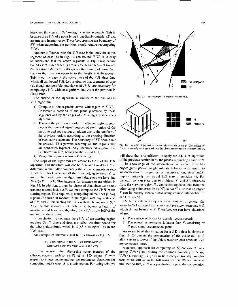
introduce the edges of S P among the active segments. This is because the I V N of a point lying immediately outside S P can assume any integer value. Therefore, crossing the boundary of SP when traversing the partition would require recomputing I V N .

Another difference with the V H case is that only the active segment of case (b) in Fig. 14 can bound I V H . It is easy to understand that the active segments in Fig. 14(a) cannot bound I V H , since when Q crosses the active segment toward the negative side there is always another family of visual half lines in the direction opposite to the family that disappears. This is not the case of the active lines of the V H algorithm, which all can bound V H . Let us observe that segments of type (a), though not possible boundaries of I V H , are necessary for computing I V N with an algorithm that visits the partition in O(n) time.

The outline of the algorithm is similar to the one of the V H algorithm.

1) Compute all the segments active with regard to I V H . 2) Construct a partition of the plane produced by these

segments and by the edges of S P using a plane-sweep algorithm.

3) Traverse the partition in order of adjacent regions, computing the intemal visual number of each region of the partition and subtracting or adding one to the number of the previous region, according to the crossing direction of each active segment. The boundary of SP should not be crossed. This permits reaching all the regions that are connected together. Any unconnected regions, that is, “holes” in SP, belong to the visual hull.

4) Merge the regions whose I V N is zero. The steps of the algorithm are similar to those of the V H

algorithm and therefore will not be described in detail. One difference is that, after computing the active segments in step 1, we can check whether all the lines belong to case (a) or not. In the former case the algorithm halts, since we have that I V H ( S P ) = SP. This happens for instance to the object in Fig. 12. In addition, it must be observed that, since we do not traverse regions inside SP, we must compute the I V H of the starting region. This requires 1) computing all the lines joining a point P chosen at random in the region with any vertex V, of SP, and 2 ) intersecting the lines with the boundary of SP. Any line that intersects SP only at V , bounds a family of intemal visual lines, and therefore the I V N is the half of the number of these lines.

In conclusion, to compute the I V N of the starting region requires O ( n 2 ) time and does not affect the time bound for the whole algorithms, which is O(n3 + mlogm), as in the V H case.

An example of intemal visual hull is shown in Fig. 15,

Iv. COMPUTING THE SILHOUE~TE-ACTIVE SURFACES OF POLYHEDRAL OBJECTS

In this section, after discussing some features of the silhouette-active surface s a ( S ) of a 3-D object S with respect to image understanding, we present an algorithm for computing s a ( S ) when S is a polyhedron. For doing this, we

‘ I /” I’ IVH(SP)SP

: II SP

Fig. 15. An example of intemal visual hull.

(a) (b)

Fig. 16. A solid S (a) and its section (b) with the plane p. The surface of S can be exactly reconstructed, but the object reconstructed is larger than S.

will show that it is sufficient to apply the 2-D V H algorithm of the previous section in all the planes supporting a face of S .

The knowledge of the silhouette-active surface of a 3-D object gives partial insight into its behavior with regard to silhouette-based recognition or reconstruction, since sa( S ) implies uniquely the visual hull (see proposition 4). For instance, we can state that two objects S’ and S”, observed from the viewing region R,, can be distinguished one from the other using silhouettes iff sa(S’) # sa(S”), or that an object S can be exactly reconstructed using volume intersection iff

The latter statement requires some remarks. In general, the visual hull of an object also consists of parts not connected to S, which do not belong to S. Therefore, we can have situations where:

s(S) = sa(S) .

1) The surface of S can be exactly reconstructed; 2) The object reconstructed is larger than S , consisting of

An example of this situation for a 3-D object is shown in Fig. 16. Of course, the computation of the visual hull of S allows us to discover if the object reconstructed contains such nonconnected parts.

A general approach for computing sa( S ) consists of computing V H ( S ) and finding the common boundary of S and V H ( S ) . Finding V H ( S ) can be a computationally complex task, as we will see in the following section. We will show in this section that, if S is a polyhedral object, the computation

S plus some unconnected parts.

1.58 IEEE TRANSACrIONS ON PATTERN ANALYSIS AND MACHINE INTELLIGENCE, VOL. 16, NO. 2, FEBRUARY 1994

The top face of the F/

mPs

VH(PS)-PS

(a) (b)

Fig. 17. The silhouette-active surface of both (a) SI and Sp and (b) a section PS of SI made by the plane containing the top face of the small cube.

of se(S) can be performed using a simple algorithm based on the 2-D algorithm of the previous section.

As in 2-D, let a visual line relative to a polyhedron S be a straight line that does not intersect S; the points lying on a visual line do not belong to the visual hull. Let n be the number of vertexes of S , which has therefore O(n) edges and faces. Finally, let p i be the plane supporting a face Fi of S and let PS; indicate the polygonal intersection of pi and S , excluding Fi itself. For finding which part of Fi, if any, lies on sa(S) , let us consider a point Q lying on F;. Q belongs to sa(S) if there is a visual line passing outside S at an infinitesimal distance from Q; this visual line therefore must be parallel to Fi. We immediately draw the following conclusion.

Proposition 13: A point Q of a face F; belongs to sa(S) iff it does not belongs to VH(PSi ) .

Therefore we can use the following simple algorithm for computing sn(S) . For each face,

1) Find PSZ, the intersection of pi and S, minus Fi itself; 2) Compute V H ( PS;) , using the 2-D algorithm described

3) Determine Fi - V H ( P S i ) , which is the part of Fi that

In more detail, the computation can be arranged as follows. First, some pruning can be performed by computing in O(n1ogn) time [21] the convex hull of S and selecting immediately for membership to s a ( S ) the faces that belong to the surface of C H ( S ) . For each of the remaining faces, the computation of PS; can be performed in O ( n ) time. Some further pruning can be performed by merging steps (2) and (3) above in the following way. When computing the active segments for the 2-D visual hull algorithm in the plane p i , we consider only the parts of the active segments that are inside Fi. The subsequent steps of the algorithm-that is, computing and visiting the partition-are therefore limited to the region enclosed by Fi, where each region whose visual number is not zero belongs to su( S ) .

Visiting each face requires computing a starting visual number. This can be performed in O(71’) time, computing all the lines joining a point of the starting region with the vertexes, and intersecting each line with the edges of SP. The number of the lines that touch S P only at a vertex, divided by two, gives the starting visual number.

For each face the time required is therefore O( n3 + k log I C ) , where k is the size of the partition of the face.

in Section 111;

belongs to sa(S) .

The time bound for the whole algorithm is therefore O(n4 + n p ) , where p is the average value of Ic log k. As an example, let us apply this algorithm to the objects SI and S2 of Fig. 2. The resulting surface is the same for both objects and is shown in Fig. 17(a). The faces of the small cube inside the concavity of S1 do not belong to the active surface, as we can verify for instance from Fig. 17(b), where a section of the object made with the plane supporting the upper face of the cube is shown. Since sw(S1) = su(Sz) , we have proven formally that we cannot tell SI from S2 using silhouettes obtained from viewpoints outside the convex hull of the objects.

Let us conclude this section observing that, unfortunately, it is not possible to extend the results just obtained for constructing a similar 2-D algorithm for computing i s a ( S ) , since the visual half-lines starting at a point whose distance from a face F; is infinitesimal need not to be parallel to Fi

v. COMPUTING VH AND I v H FOR POLYHEDRAL OBJECTS

In this section we tackle the problem of computing the visual hulls of unrestricted polyhedra. For doing this, in V-A we extend in 3-D the concept of visual number. In V-B we show that 3-D regions with different visual numbers are separated by planar or quadric surfaces, which can be easily computed from the geometry of the object. Instances of visual hulls of simple polyhedra are presented in V-C. The relationship between visual hull and aspect graph of polyhedra is discussed in V-D. A general algorithm for computing the visual hull of a polyhedron is presented in V-E. As in the 2-D case, the algorithm constructs a partition of the space into zones containing points with the same 3-D visual number, computes the visual numbers, and selects all the zones whose visual number is zero. Finally, in V-F the features of the internal visual hull of a polyhedron are briefly discussed and an algorithm for its computation is outlined.

A . The 3-0 Visual Number

For constructing a general algorithm able to compute the visual hull of a polyhedron S , we will extend in 3-D the concept of visual number. V N 3 D ( Q , S ) , the 3-D visual number of a point Q with respect to S , should be defined in such a way that the following hold true.

1) Its value determines the membership of Q to V H ( S ) . 2) It is possible to compute from the geometry of S a

partition of R3 into regions containing points with the same visual number.


(a) (b)

Fig. 18. Examples of two situations in whlch an edge of the visual cone disappears. In (a) E, and E, share the vertex T..; In (b) they do not have a common vertex.

Let us consider a point Q 4 S and all the visual lines relative to S passing through P. These lines fill an infinite conical volume that we define as the visual cone of Q relative to s.

The boundary of the visual cone consists of a number of infinite planar faces that will be referred to as visual angles. Each visual angle is generated by the lines passing through P and tangent to S at an edge E,, or part of it. We define the 3-D visual number as follows.

Definition 6: VN3D(Q. S ) is the number of edges (or faces) of the visual cone of Q relative to S.

It is clear that this definition satisfies the above requirement 1. We have in fact the following.

Proposition 14: V N 3 D ( Q , S ) = 0 if and only if Q E V H ( S ) .

In the following we will show that definition 6 also satisfies requirement 2.

B . The Active Su$aces

Let the active surfaces, as the active lines in 2-D, be the surfaces that contain active segments. The active segments are parts of surfaces that separate points of R3 whose V N 3 D are different, and are therefore potential boundaries of V H ( S).

Consider an edge E of the visual cone of a point P relative to S, and let E, and E3 be the edges of S which originate the visual angles that intersect at E. Two cases are possible.

1 ) E, and E3 have a common vertex V . 2) E, and E3 have no common vertex. For finding which are the active surfaces, we will imagine

continuously displacing P until the edge E is removed from the boundary of the visual cone.

In both cases 1 and 2 the edge E disappears when it intersects s at an edge Ek. The difference is that in case I ) , E is the line passing through P and V ; in case 2), the edge E intersects E, and E3 at different points for each position of P. Examples of these two situations are shown in Fig. 18(a) and (b), respectively, as seen from a point lying on E on one side of E,, E3 and Ek.

Let us consider case 1. The active surface for this case is generated by all the lines that pass through the vertex V and the edge Ek (or part of it) and do not share with S any other point, but for the case in which V and Ek belong to the same face of S. If this happens, the lines that form the active surface share some segment with this face. Let the active infinite planar surfaces relative to case 1 be the V E surfaces.

In case 2, the active surface is generated by all the lines tangent to S at three edges E,, E3, and Ek. It is a curved

surface. In fact, from basic 3-D analytic geometry we have that the lines passing through three lines skew to each other form a hyperboloid of one sheet or a hyperbolic paraboloid. The second case takes place when the three lines are all parallel to a plane. We define these curved active surfaces as E E E surfaces.

In conclusion, we have found two kinds of surfaces that are active with respect to V N 3 D and are therefore potential boundaries of V H ( S ) . All these surfaces are ruled surfaces, generated by lines tangent to S and sharing with it at least two points. A main result of the previous discussion is as follows.

Proposition 15: The boundary of the visual hull of a planar- face object in general is not planar and consists of planar and quadric patches.

Actually, not all the V E and E E E surfaces that are active with respect to V N 3 D can also be boundaries of V H . As an example, consider the two cases of Fig. 19(a) and (c). The edges of S that determine the active surfaces are observed from a viewpoint lying on a line L of the active surface and are projected onto an image plane normal to this line. In the first case, relative to a V E surface, let us analyze the situation in the plane q passing through L, whose trace in the image plane is shown in Fig. 19(a). This situation is shown in Fig. 19(b), where the dotted lines indicate visual lines passing on both sides of every part of L. Therefore, L and the whole V E surface cannot belong to the boundary of V H ( S ) . In the second case we analyze three 2-D situations, in three planes a, b and c passing through L. It is clear (see Fig. 19(d)) that in plane a we can construct visual lines on both sides of the external segments of L, in plane b on both sides of the segment E2E3, and in plane c on both sides of the segment ElEz. Therefore neither L nor the E E E surface that contains L can be boundaries of V H ( S ) . We will not analyze here in detail all the possible cases, since this is not necessary for the brute- force algorithm for computing V H ( S ) that we will present later in this paper.

C. Examples of Visual Hulls of Simple Polyhedra

This subsection is devoted to clarifying the items presented so far by discussing some simple examples. Let us consider first the polyhedron S3, one of the objects in Fig. 3. In Fig. 20(a) S3 is shown together with the part of the active surface due to E1 and VI that is inside the convex hull. When a point crosses this surface in the direction shown in figure, its V N 3 D changes from 0 to 3. In fact, a visual cone is generated that is bounded by the three visual angles relative to E l , Ez, and E3. Therefore, this surface is a boundary of V H ( S 3 ) , which is shown in Fig. 20(b). In the same figure another active surface is shown. It is the V E surface due to E3 and V3. Crossing this surface in the direction shown in the figure, V N S D is incremented by one, since the visual cone acquires a new visual angle relative to E4.

Let us now consider the objects SI and S2 of Fig. 2. We have already found their silhouette-active surface (see Fig. 17). It is not difficult to determine the visual hull shown in Fig. 21(a). There are many active surfaces, some of them overlapping because of parallel edges. For instance, the surface pointed at by the arrow in the figure is due to two active V E

160 IEEE TRANSACTIONS ON PA'ITERN ANALYStS AND MACHINE INTELLIGENCE, VOL. 16, NO. 2. FEBRUARY 1994

E --:: : * - ---a= : : L section made by - - - the piane 9

E1 E2 E3 L ,- section made by a ~e section made by b

,-L section made by c

I I

(C? (d?

Fig. 19. (a) A 1.E surface and its section made by (b) the plane (1, showing that the surface cannot bound l * H ( S ) . Also, the EEE surface in (c) cannot bound LrH(S), as is shown in (d).

v2

v3 V3

ACTIVE SURFACKS

(a? (b)

which adds 1 to 1-530. Fig. 20. The polyhedron S3 and an active surface (a) that adds three to 1 . ~ V 3 0 : I.H(S2) and another active surface (b),

0 ACTIVE SURFACES (b) (c)

Fig. 21. (a) The visual hull of both SI and Sa. The face pointed at by the arrow is generated by two partially overlapping active surfaces, shown in (b) and (c).

surfaces generated by the pairs vertex-edge (VI, E l ) , (V,, E4) (see Fig. 21(b) and (c)). Crossing this surface in the direction opposite to the arrow changes V N 3 D from 0 to 4.

Another object with a slightly more complex concavity is shown in Fig. 22(a). To determine by inspection its visual hull, shown in Pig. 22(b), takes some more reflection.

The objects so far considered have no lines tangent at three points, and therefore no cubic patch belongs to the boundary of their visual hulls. A cubic patch, on the other hand, is present in the boundary of the visual hull (Fig. 23(b)) of the polyhedron in Fig. 23(a). The boundary of the visual hull consists of four

patches, PI , P2, P3. and Pd, in addition to the silhouette- active surface. Some of the planar patches are generated by more than one active surface because of parallel edges. P3 is a segment of the quadric surface generated by the lines tangent at El, E2, and E,.

D. The Visual Hull and the Aspect Graphs

In this subsection we will discuss briefly the relationship between the visual hull and the aspect graph. The aspect graph and its computation have recently become popular research topics. In short, the aspect graph of a 3-D object stores at


(a) (b)

Fig. 22. (a) An object with a more complex concavity and (b) its visual hull. Some dotted lines of construction are also shown.

(a) (b)

Fig, 23. (a) A polyhedron S and (b) its visual hull. F3 is a segment of a quadric surface produced by the lines tangent to S at the edges E1 , Ez , and E3.

the vertexes of a graph all the topologically distinct line drawings of an object. The edges of the graph represent visual events-that is, topological changes in the views. Algorithms for computing the aspect graph have been given for polygons, polyhedra, solids of revolution, and other curved objects. For further details on this matter, the interested reader is referred to [22] and [24], quoted elsewhere in this paper, and to the survey paper [25] of Bowyer and Dyer.

Here we will point out that the active surfaces that we have found in relation to the 3-D visual number are well known in the field of the computation of the aspect graph of polyhedral objects, In fact, V E and E E E surfaces are a subset of the surfaces that divide the viewing space into regions such that each viewpoint of the region gives topologically equivalent views. More specifically, the active surfaces relative to V N 3 D are the same surfaces relative to the aspect graph that are due to the visual events on the boundary of the line drawing of the polyhedron. We could also say that these surfaces generate the silhouette or contour aspect graph of an object.

E . A Brute-Force Algorithm for Computing the Visual Hull

be performed as follows. The computation of the visual hull of a polyhedron S can

1) Compute all the potentially active surfaces. 2) Construct the partition of R3 generated by the potentially

3) Compute V N 3 D for each cell of the partition. 4) Merge together all the cells whose visual number is zero.

In the first step 0 ( ~ r ’ ) surfaces are computed in 0(n3) time, con4idering O ( n 2 ) V - E pairs and O(n3) E E E triplets.

active surfaces.

m algebraic surfaces divide R3 in O(m3) cells. In our case, therefore, the partition has O(ng) cells, faces, edges, and vertexes. The construction of the partition can be performed in O(n9 log n) time using an incremental algorithm, as shown by Plantinga and Dyer in [24].

The V N 3 D of a point Q chosen at random in a cell can be computed as follows. Compute first in O(n2) time the polygonal intersections INT , of O ( n ) potential visual angle with the O(n) faces of S. For each visual angle, compute the 2- D visual number of Q relative to INTi. V N 3 D is obtained by adding up all the 2-D visual numbers. Since the computation of each 2-D visual number takes O(n2) time, the V N 3 D of each zone is obtained in 0(n3) time.

The bound for the computation time of step 3 results therefore in O(nl2) , which is also the bound for the whole algorithm, since step 4 can be performed in time linear with the size of the partition. We will not mention some trivial pruning actions that do not affect the time bound of the algorithm.

F. The Computation of the Internal Visual Hull We can deal with the internal visual hull of a polyhedral

object S as we did with the external visual hull, introducing some suitable modifications. Let us first define the internal 3- D visual number. Consider a point Q $! S and all the visual half-lines relative to S , starting at P. A visual half-line is a half-line that does not intersect S. These lines fill an infinite half-conical volume that we define to be the visual halfcone of Q relative to S.

I’he boundary of the visual half-cone, which is coincident with the circumscribed cone, consists of a number of infinite planar faces that will be referred to as visual halfangles. Each visual half-angle is generated by the half-lines starting at Q and tangent to S at an edge E,, or part of it. We give the following definition.

Definition 7: IVN3D(Q, S ) , the intemal 3-D visual number of a point Q relative to S , is the number of edges (or faces) of the circumscribed cone.

The following proposition becomes clear. Proposition 15: IVN3D(Q, S ) = 0 if and only if Q E

I V H ( S ) . Since the potentially active surfaces relative to I V N 3 D

are the same surfaces of the V N 3 D case, we can use the same brute-force algorithm for computing I V H , the only difference being the computation of IVN3D(Q, S ) instead of V N 3 D ( Q , S ) for a point Q of each cell. It is easy to see that this computation can be performed by adding O(n) 2-D intemal visual numbers, each relative to Q and to the intersections of S with each potential visual half-angle. Therefore the computation of I V N 3 D takes O(n3) time, so the overall time bound of the algorithm is 0(nl2) again.

VI. CONCLUSION

We have addressed the problem of finding which parts of a nonconvex object are relevant for silhouette-based image understanding. A new geometric entity, the visual hull, has been introduced. We have shown that the knowledge of the visual hull of an object provides a full solution to this problem. The visual hull V H ( S , R) of an object S is the maximal object


silhouette-equivalent to S with respect to a viewing region R. V H ( S , R) also is the closest approximation of S that can be obtained applying the volume intersection technique with viewpoints belonging to R.

Analyzing the possible viewing regions, the existence of a main case relative to the external, or natural, visual hull V H ( S ) has been recognized. V H ( S ) is the visual hull relative to the region R,, which is complementary to the convex hull of S; it also is the visual hull of any viewing region that is a subset of R, and completely encloses S. In addition, the visual hull relative to any region that is a subset of R, can be constructed starting from V H ( S ) .

The case of the largest possible viewing region, bounded by S itself, has been also considered. The corresponding internal visual hull I V H ( S ) also allows us to find which features of the surface of S cannot appear on any image of the object obtained from viewpoints not belonging to the convex hull.

Two efficient algorithms have been described for computing the visual hull and the intemal visual hull of 2-D objects. These algorithms divide the plane into regions that either entirely belong to the visual hulls or to its complement. The time bound of both these algorithms is O(n3 + mlogm) , where rn is the size of the partition and n is the number of algebraic curves defining the boundary of the object. The 2-D algorithms allow us to find the visual hulls of 23 - D sweep solids and provide the basis for an algorithm described elsewhere for dealing with solids of revolution.

The silhouette-active surface of a 3-D object gives a partial insight into the behavior of the object under silhouette-based recognition algorithms. For instance, two objects can be discriminated using silhouettes if their silhouette-active surfaces are different. We have shown that for a polyhedron the external silhouette-active surface can be computed applying the 2-D algorithm in each of the planes supporting a face of S. No similar algorithm is possible for the internal silhouette-active surface.

We have also addressed the problem of computing the whole extemal visual hull and the internal visual hull of a general polyhedron. By extending in 3-D some concepts used in the 2-D algorithm, we have been able to find which surfaces are potential boundaries of both visual hulls. The result is planar and ruled quadric surfaces, so that the boundary of the visual hull of a general polyhedron may be nonplanar. These surfaces also are a subset of the surfaces used by the algorithms for computing the aspect graph of a polyhedron. Brute-force algorithms for computing in O(nl*) time the visual hulls of general polyhedra have been given.

To be able to compute the visual hull of objects with curved surfaces would enhance the effectiveness of the visual hull idea. This topic is currently under investigation, together with efficient algorithms for the polyhedral case.

REFERENCES

[I1 J. Aloimonos, “Visual shape computation,” IEEE Proc., vol. 76, no. 8,

[21 P. J. Besl and R. C. Jain, “Three-dimensional object recognition,”

[31 C. Chien and J. K. Agganval. “Model reconstruction and shape recogni-

pp. 899-916, 1988.

Comput. Surveys. vol. 17, pp. 75-145, 1985.

tion from occluding contours,” IEEE Trans. Part. Anal. Machine Intell.,

T. P. Wallace and P. A. Wintz, “An efficient three-dimensional aircraft recognition algorithm using normalized Fourier descriptors,” Comput. Graphics Image Processing. vol 13, pp. 99-126, 1980. M. Hebert and T. Kanade, “The 3-D profile method for object recognition,” in Proc. IEEE Computer Sociery Conf Computer Vision and Pattern Recognition. pp. 458-463, June 1985. A. P. Reeves et al., “Three-dimensional shape analysis using moments and Fourier descriptors,” IEEE Trans. Putt. Anal. Machine Intell.. vol.

S. A. Dudani et al., “Aircraft identification by moment invariants,” IEEE Trans. Compur., vol. C-26, pp. 39-46, 1981. Y. F. Wang, M. J. Magee, and J. K. Agganval, “Matching three- dimensional objects using silhouettes,” IEEE Trans. Putt. Anal. Machine Intell., vol. PAMI-6, pp. 513-518, 1984. M. Brady and A. Yuille, “An extremum principle for shape from contour,” IEEE Trans. Patt. Anal. Machine Intell., vol. PAMI-6, pp. 288-301, 1984. W. N. Martin and J. K. Aggarwal, “Volumetric description of objects from multiple views,” IEEE Trans. Putt. Anal. Machine Intell., vol.

P. Srinivasan et al., “Computational geometric methods in volumetric intersection for 3D reconstruction,” Parr. Recogn., vol. 23, pp. 843-857, 1990. M. Potemesil, “Generating octree models of 3D objects from their silhouettes in a sequence of images,” Comput. Vision Graphics Image Processing, vol. 40, pp. 1-29, 1987. H. Noborio et al., “Construction of the octree approximating three- dimensional objects by using multiple views,” IEEE Trans. Part. Anal. Machine Infell., vol. 10, pp. 769-782, 1988. C. H. Chien and J. K. Agganval, “Volume/surface Octrees for the representation of three-dimensional objects,” Comput. Vision, Graphics and Image Processing. vol. 36, pp. 1W113, 1986. V. Cappellini er al., “From multiple views to object recognition,” IEEE Trans. Circuits Sysf., vol. CS-34, pp. 1344-1350, 1987. N. Ahuja and J. Veenstra, “Generating octrees from object silhouettes in orthographic views,” IEEE Trans. Putt. Anal. Machine Intell., vol. 11, pp. 137-149, 1989. T. H. Hong and M. Schneier, “Describing a robot’s workspace using a sequence of views from a moving camera,” IEEE Trans. Parr. Anal. Machine Infell.. vol. PAMI-7, pp. 721-726, 1985. K. Shanmukh and A. K. Pujari, “Volume intersection with optimal set of directions,” Part. Recogn. Lett., vol. 12, pp. 165-170, 1991. A. Laurentini, “The visual hull: A new tool for contour-based image understanding,” in Proc. 7th Scandinavian Conf Image Analysis, pp. 993-1002, 1991. -. “The visual hull of solids of revolution,” in Proc. 11th IAPR, The Hague, Netherlands, Aug. 30-Sept. 3, 1992, pp. 720-724. F. Preparata and M. Shamos, Compufafional Geometry. New York: Springer, 1985 Z. Gigus, J. Canny, and R. Seidel, “Efficiently computing and repre- senting aspect graphs of polyhedral objects,” IEEE Trans. Putt. Anal. Machine Infell., vol. 13, pp. 542-551, June 1991. S. Baase, Compurer Algorithms. H. Plantinga and C. R. Dyer, “Visibility, occlusion and the aspect graph,” In t . J. Comput. Vision, vol. 5, no. 2, pp. 137-160, 1990. K. W. Bowyer and C. R. Dyer, “Aspect graphs: An introduction and survey of recent results,” Int. J. Imaging Syst. Techno[., vol. 2, pp. 315-328, 1990.

vol. 11, pp. 372-389, 1989.

IO, pp. 937-943, 1988.

PAMIJ, pp. 150-158, 1983.

New York: Addison-Wesley, 1988.

Aldo Laurentini was bom in Genova, Italy, on November 13, 1940. He received the degree in In- gegneria Elettronica from the Politecnico di Milano, Milan, Italy, in 1963.

In 1965 he joined the Politecnico di Torino, Turin, Italy, where he is Professor of Computer Science in the Dipartimento di Automatica ed Informatica. His current research interests are in the areas of computer vision, computer graphics, and document understanding.

silhouette

Documents

Transcript of silhouette