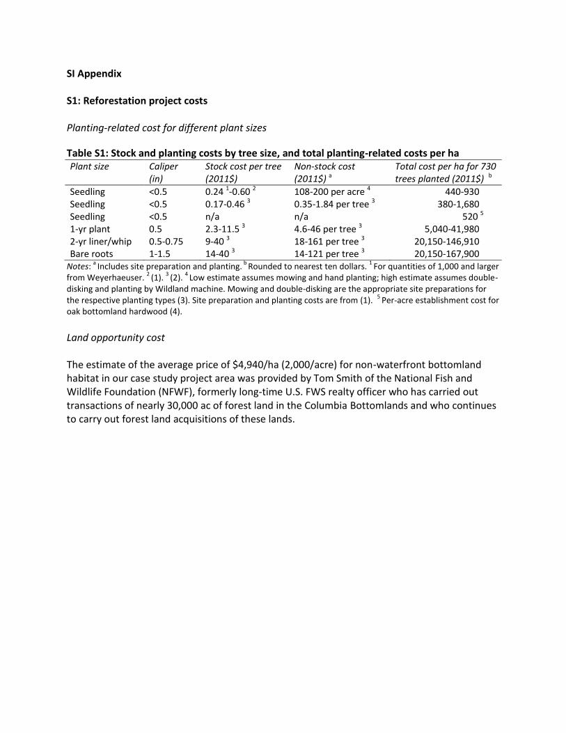
SI Appendix S1: Reforestation project costs Planting-related cost for different plant sizes

Table S1: Stock and planting costs by tree size, and total planting-related costs per ha Plant size Caliper

(in) Stock cost per tree (2011$)

Non-stock cost (2011$) a

Total cost per ha for 730 trees planted (2011$) b

Seedling <0.5 0.24 1-0.60 2 108-200 per acre 4 440-930 Seedling <0.5 0.17-0.46 3 0.35-1.84 per tree 3 380-1,680 Seedling <0.5 n/a n/a 520 5

1-yr plant 0.5 2.3-11.5 3 4.6-46 per tree 3 5,040-41,980 2-yr liner/whip 0.5-0.75 9-40 3 18-161 per tree 3 20,150-146,910 Bare roots 1-1.5 14-40 3 14-121 per tree 3 20,150-167,900

Notes: a

Includes site preparation and planting. b

Rounded to nearest ten dollars. 1

For quantities of 1,000 and larger from Weyerhaeuser.

2 (1).

3 (2).

4 Low estimate assumes mowing and hand planting; high estimate assumes double-

disking and planting by Wildland machine. Mowing and double-disking are the appropriate site preparations for the respective planting types (3). Site preparation and planting costs are from (1).

5 Per-acre establishment cost for

oak bottomland hardwood (4).

Land opportunity cost The estimate of the average price of $4,940/ha (2,000/acre) for non-waterfront bottomland habitat in our case study project area was provided by Tom Smith of the National Fish and Wildlife Foundation (NFWF), formerly long-time U.S. FWS realty officer who has carried out transactions of nearly 30,000 ac of forest land in the Columbia Bottomlands and who continues to carry out forest land acquisitions of these lands.

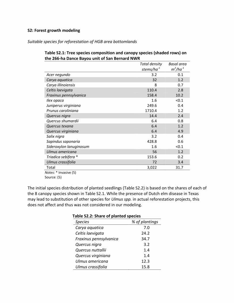
S2: Forest growth modeling Suitable species for reforestation of HGB area bottomlands

Table S2.1: Tree species composition and canopy species (shaded rows) on the 266-ha Dance Bayou unit of San Bernard NWR Total density Basal area

stems/ha-1 m2/ha-1

Acer negundo 3.2 0.1 Carya aquatica 32 1.2 Carya illinoiensis 8 0.7 Celtis laevigata 110.4 2.8 Fraxinus pennsylvanica 158.4 10.2 Ilex opaca 1.6 <0.1 Juniperus virginiana 249.6 0.4 Prunus caroliniana 1710.4 1.2 Quercus nigra 14.4 2.4 Quercus shumardii 6.4 0.8 Quercus texana 6.4 1.2 Quercus virginiana 6.4 4.9 Salix nigra 3.2 0.4 Sapindus saponaria 428.8 0.6 Sideroxylon lanuginosum 1.6 <0.1 Ulmus americana 56 1.2 Triadica sebifera * 153.6 0.2 Ulmus crassifolia 72 3.4

Total 3,022 31.7 Notes: * Invasive (5) Source: (5)

The initial species distribution of planted seedlings (Table S2.2) is based on the shares of each of the 8 canopy species shown in Table S2.1. While the presence of Dutch elm disease in Texas may lead to substitution of other species for Ulmus spp. in actual reforestation projects, this does not affect and thus was not considered in our modeling.

Table S2.2: Share of planted species

Species % of plantings

Carya aquatica 7.0 Celtis laevigata 24.2 Fraxinus pennsylvanica 34.7 Quercus nigra 3.2 Quercus nuttallii 1.4 Quercus virginiana 1.4 Ulmus americana 12.3 Ulmus crassifolia 15.8

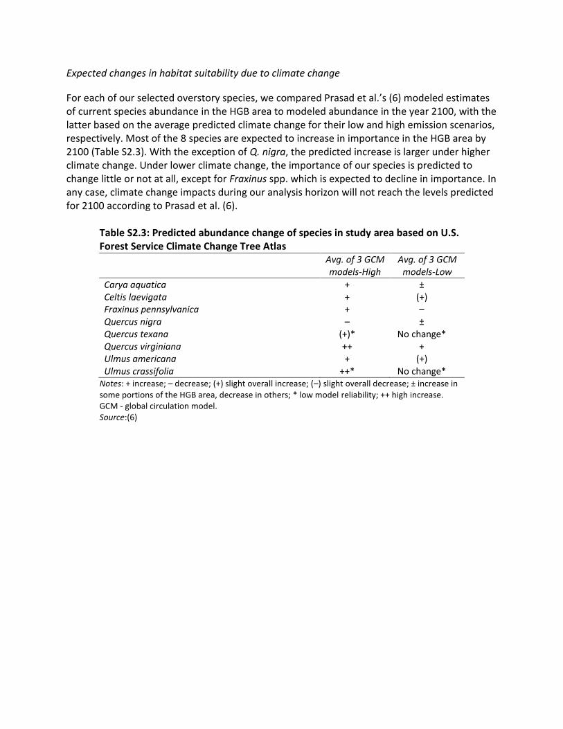
Expected changes in habitat suitability due to climate change

For each of our selected overstory species, we compared Prasad et al.’s (6) modeled estimates of current species abundance in the HGB area to modeled abundance in the year 2100, with the latter based on the average predicted climate change for their low and high emission scenarios, respectively. Most of the 8 species are expected to increase in importance in the HGB area by 2100 (Table S2.3). With the exception of Q. nigra, the predicted increase is larger under higher climate change. Under lower climate change, the importance of our species is predicted to change little or not at all, except for Fraxinus spp. which is expected to decline in importance. In any case, climate change impacts during our analysis horizon will not reach the levels predicted for 2100 according to Prasad et al. (6).

Table S2.3: Predicted abundance change of species in study area based on U.S. Forest Service Climate Change Tree Atlas Avg. of 3 GCM

models-High Avg. of 3 GCM

models-Low

Carya aquatica + ± Celtis laevigata + (+) Fraxinus pennsylvanica + – Quercus nigra – ± Quercus texana (+)* No change* Quercus virginiana ++ + Ulmus americana + (+) Ulmus crassifolia ++* No change*

Notes: + increase; – decrease; (+) slight overall increase; (–) slight overall decrease; ± increase in some portions of the HGB area, decrease in others; * low model reliability; ++ high increase. GCM - global circulation model. Source:(6)

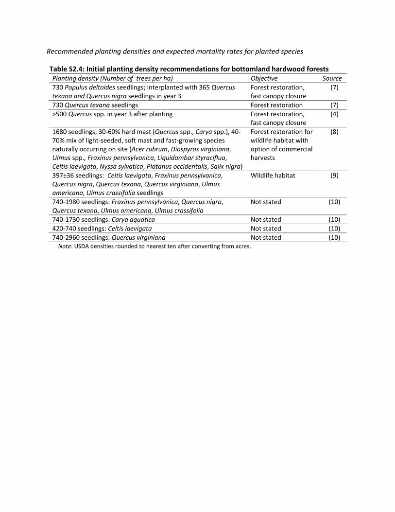
Recommended planting densities and expected mortality rates for planted species

Table S2.4: Initial planting density recommendations for bottomland hardwood forests Planting density (Number of trees per ha) Objective Source

730 Populus deltoides seedlings; interplanted with 365 Quercus texana and Quercus nigra seedlings in year 3

Forest restoration, fast canopy closure

(7)

730 Quercus texana seedlings Forest restoration (7)

>500 Quercus spp. in year 3 after planting Forest restoration, fast canopy closure

(4)

1680 seedlings; 30-60% hard mast (Quercus spp., Carya spp.), 40-70% mix of light-seeded, soft mast and fast-growing species naturally occurring on site (Acer rubrum, Diospyros virginiana, Ulmus spp., Fraxinus pennsylvanica, Liquidambar styraciflua, Celtis laevigata, Nyssa sylvatica, Platanus occidentalis, Salix nigra)

Forest restoration for wildlife habitat with option of commercial harvests

(8)

397±36 seedlings: Celtis laevigata, Fraxinus pennsylvanica, Quercus nigra, Quercus texana, Quercus virginiana, Ulmus americana, Ulmus crassifolia seedlings

Wildlife habitat (9)

740-1980 seedlings: Fraxinus pennsylvanica, Quercus nigra, Quercus texana, Ulmus americana, Ulmus crassifolia

Not stated (10)

740-1730 seedlings: Carya aquatica Not stated (10)

420-740 seedlings: Celtis laevigata Not stated (10)

740-2960 seedlings: Quercus virginiana Not stated (10) Note: USDA densities rounded to nearest ten after converting from acres.

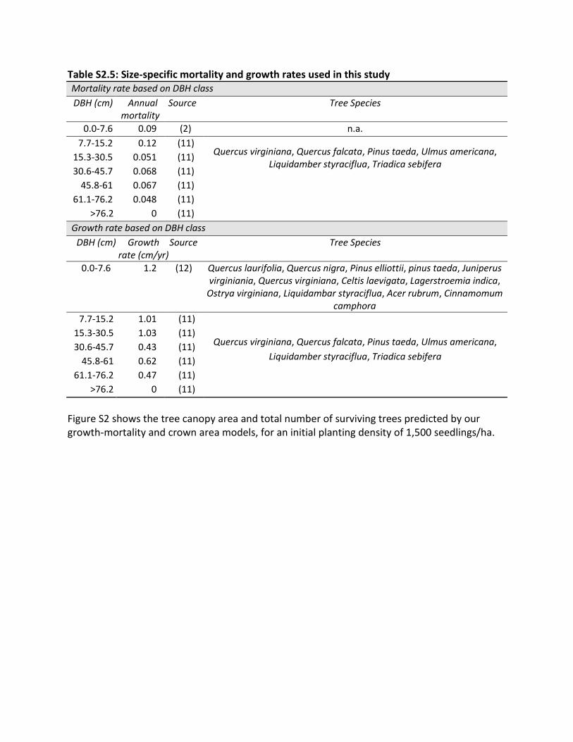
Table S2.5: Size-specific mortality and growth rates used in this study Mortality rate based on DBH class

DBH (cm) Annual mortality

Source Tree Species

0.0-7.6 0.09 (2) n.a.

7.7-15.2 0.12 (11) Quercus virginiana, Quercus falcata, Pinus taeda, Ulmus americana,

Liquidamber styraciflua, Triadica sebifera 15.3-30.5 0.051 (11)

30.6-45.7 0.068 (11)

45.8-61 0.067 (11)

61.1-76.2 0.048 (11)

>76.2 0 (11)

Growth rate based on DBH class

DBH (cm) Growth rate (cm/yr)

Source Tree Species

0.0-7.6 1.2 (12) Quercus laurifolia, Quercus nigra, Pinus elliottii, pinus taeda, Juniperus virginiania, Quercus virginiana, Celtis laevigata, Lagerstroemia indica,

Ostrya virginiana, Liquidambar styraciflua, Acer rubrum, Cinnamomum camphora

7.7-15.2 1.01 (11)

Quercus virginiana, Quercus falcata, Pinus taeda, Ulmus americana,

Liquidamber styraciflua, Triadica sebifera

15.3-30.5 1.03 (11)

30.6-45.7 0.43 (11)

45.8-61 0.62 (11)

61.1-76.2 0.47 (11)

>76.2 0 (11)

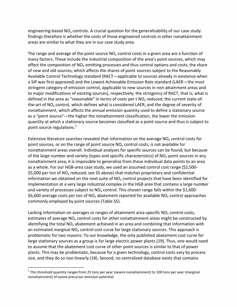
Figure S2 shows the tree canopy area and total number of surviving trees predicted by our growth-mortality and crown area models, for an initial planting density of 1,500 seedlings/ha.

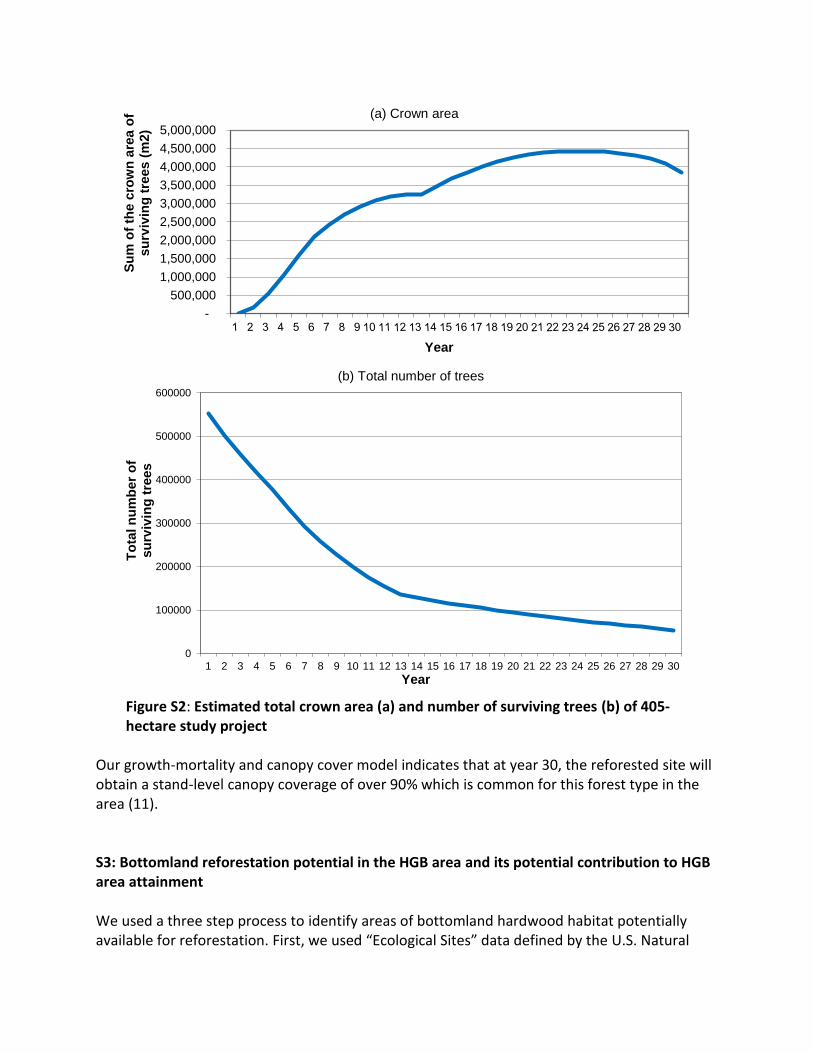
Figure S2: Estimated total crown area (a) and number of surviving trees (b) of 405-hectare study project

Our growth-mortality and canopy cover model indicates that at year 30, the reforested site will obtain a stand-level canopy coverage of over 90% which is common for this forest type in the area (11). S3: Bottomland reforestation potential in the HGB area and its potential contribution to HGB area attainment We used a three step process to identify areas of bottomland hardwood habitat potentially available for reforestation. First, we used “Ecological Sites” data defined by the U.S. Natural

-

500,000

1,000,000

1,500,000

2,000,000

2,500,000

3,000,000

3,500,000

4,000,000

4,500,000

5,000,000S

um

of

the c

row

n a

rea o

f su

rviv

ing

tre

es (

m2)

Year

(a) Crown area

0

100000

200000

300000

400000

500000

600000

1 2 3 4 5 6 7 8 9 10 11 12 13 14 15 16 17 18 19 20 21 22 23 24 25 26 27 28 29 30

To

tal n

um

ber

of

su

rviv

ing

tre

es

Year

(b) Total number of trees

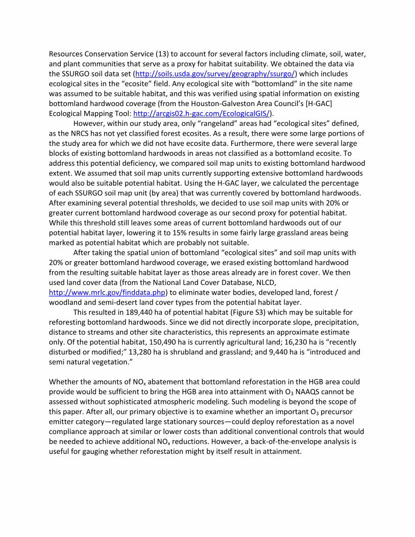
Resources Conservation Service (13) to account for several factors including climate, soil, water, and plant communities that serve as a proxy for habitat suitability. We obtained the data via the SSURGO soil data set (http://soils.usda.gov/survey/geography/ssurgo/) which includes ecological sites in the “ecosite” field. Any ecological site with “bottomland” in the site name was assumed to be suitable habitat, and this was verified using spatial information on existing bottomland hardwood coverage (from the Houston-Galveston Area Council’s [H-GAC] Ecological Mapping Tool: http://arcgis02.h-gac.com/EcologicalGIS/).

However, within our study area, only “rangeland” areas had “ecological sites” defined, as the NRCS has not yet classified forest ecosites. As a result, there were some large portions of the study area for which we did not have ecosite data. Furthermore, there were several large blocks of existing bottomland hardwoods in areas not classified as a bottomland ecosite. To address this potential deficiency, we compared soil map units to existing bottomland hardwood extent. We assumed that soil map units currently supporting extensive bottomland hardwoods would also be suitable potential habitat. Using the H-GAC layer, we calculated the percentage of each SSURGO soil map unit (by area) that was currently covered by bottomland hardwoods. After examining several potential thresholds, we decided to use soil map units with 20% or greater current bottomland hardwood coverage as our second proxy for potential habitat. While this threshold still leaves some areas of current bottomland hardwoods out of our potential habitat layer, lowering it to 15% results in some fairly large grassland areas being marked as potential habitat which are probably not suitable.

After taking the spatial union of bottomland “ecological sites” and soil map units with 20% or greater bottomland hardwood coverage, we erased existing bottomland hardwood from the resulting suitable habitat layer as those areas already are in forest cover. We then used land cover data (from the National Land Cover Database, NLCD, http://www.mrlc.gov/finddata.php) to eliminate water bodies, developed land, forest / woodland and semi-desert land cover types from the potential habitat layer.

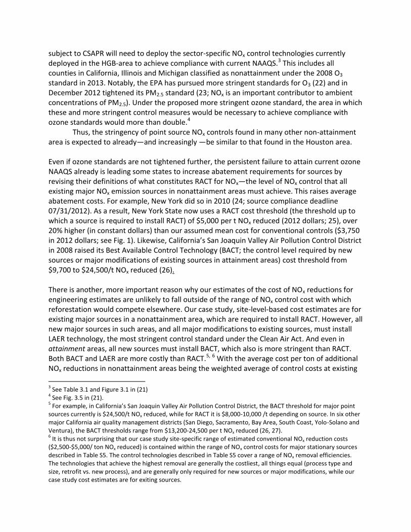
This resulted in 189,440 ha of potential habitat (Figure S3) which may be suitable for reforesting bottomland hardwoods. Since we did not directly incorporate slope, precipitation, distance to streams and other site characteristics, this represents an approximate estimate only. Of the potential habitat, 150,490 ha is currently agricultural land; 16,230 ha is “recently disturbed or modified;” 13,280 ha is shrubland and grassland; and 9,440 ha is “introduced and semi natural vegetation.” Whether the amounts of NOx abatement that bottomland reforestation in the HGB area could provide would be sufficient to bring the HGB area into attainment with O3 NAAQS cannot be assessed without sophisticated atmospheric modeling. Such modeling is beyond the scope of this paper. After all, our primary objective is to examine whether an important O3 precursor emitter category—regulated large stationary sources—could deploy reforestation as a novel compliance approach at similar or lower costs than additional conventional controls that would be needed to achieve additional NOx reductions. However, a back-of-the-envelope analysis is useful for gauging whether reforestation might by itself result in attainment.

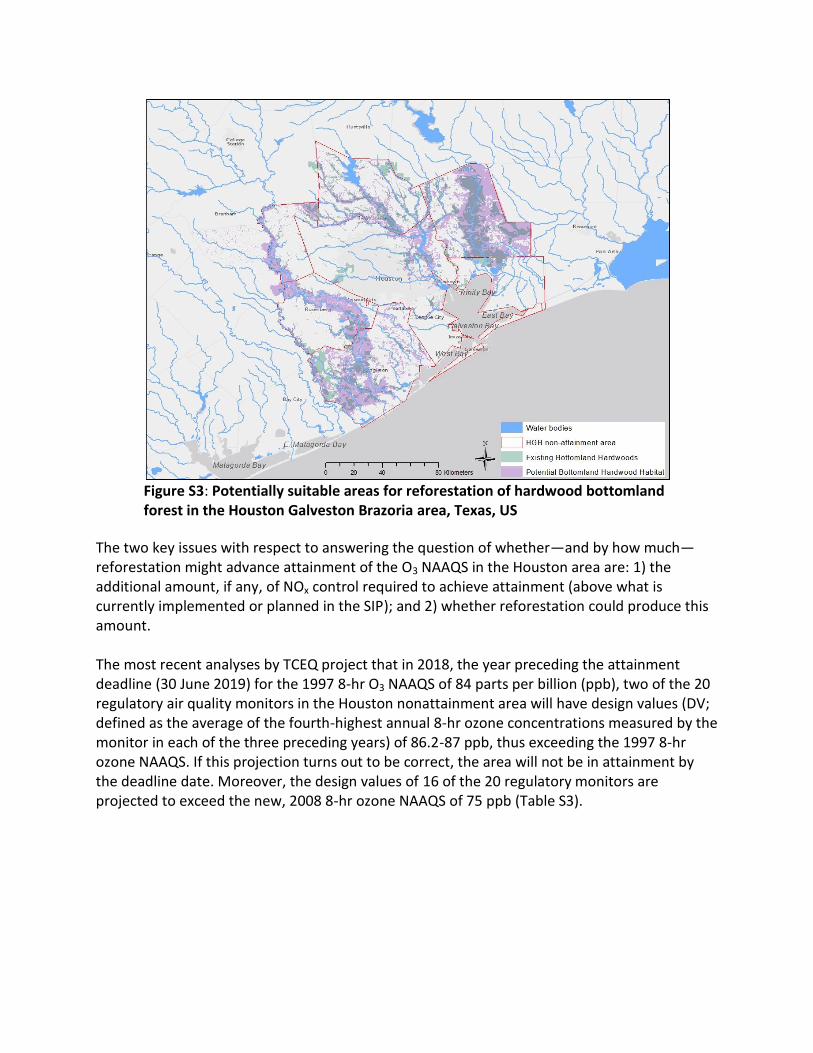
Figure S3: Potentially suitable areas for reforestation of hardwood bottomland forest in the Houston Galveston Brazoria area, Texas, US

The two key issues with respect to answering the question of whether—and by how much—reforestation might advance attainment of the O3 NAAQS in the Houston area are: 1) the additional amount, if any, of NOx control required to achieve attainment (above what is currently implemented or planned in the SIP); and 2) whether reforestation could produce this amount. The most recent analyses by TCEQ project that in 2018, the year preceding the attainment deadline (30 June 2019) for the 1997 8-hr O3 NAAQS of 84 parts per billion (ppb), two of the 20 regulatory air quality monitors in the Houston nonattainment area will have design values (DV; defined as the average of the fourth-highest annual 8-hr ozone concentrations measured by the monitor in each of the three preceding years) of 86.2-87 ppb, thus exceeding the 1997 8-hr ozone NAAQS. If this projection turns out to be correct, the area will not be in attainment by the deadline date. Moreover, the design values of 16 of the 20 regulatory monitors are projected to exceed the new, 2008 8-hr ozone NAAQS of 75 ppb (Table S3).

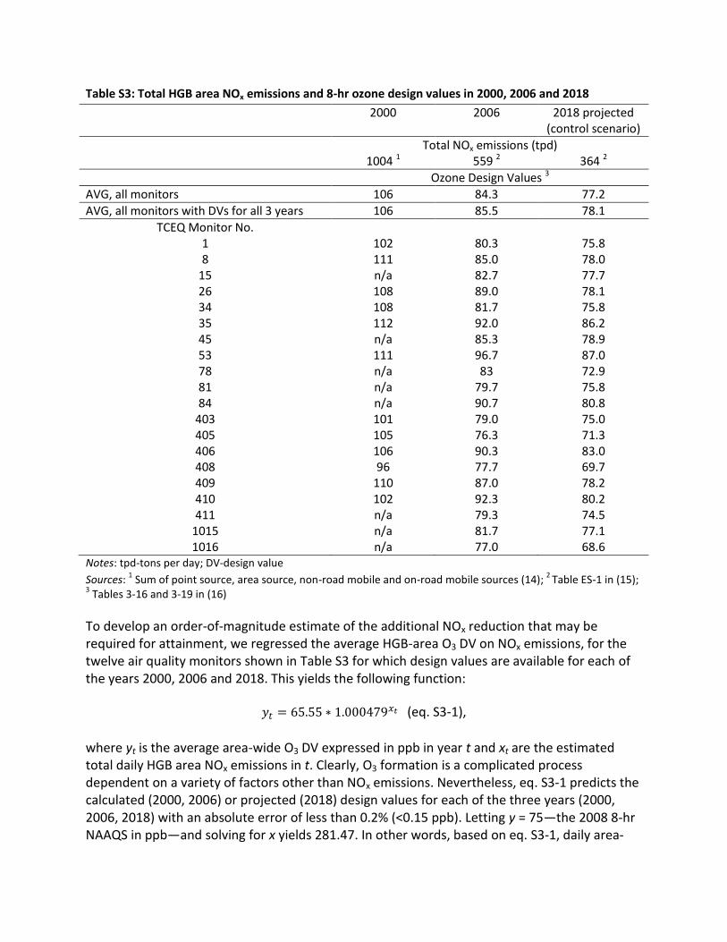
Table S3: Total HGB area NOx emissions and 8-hr ozone design values in 2000, 2006 and 2018

2000 2006 2018 projected (control scenario)

Total NOx emissions (tpd) 1004 1 559 2 364 2

Ozone Design Values 3

AVG, all monitors 106 84.3 77.2

AVG, all monitors with DVs for all 3 years 106 85.5 78.1

TCEQ Monitor No. 1 102 80.3 75.8 8 111 85.0 78.0

15 n/a 82.7 77.7 26 108 89.0 78.1 34 108 81.7 75.8 35 112 92.0 86.2 45 n/a 85.3 78.9 53 111 96.7 87.0 78 n/a 83 72.9 81 n/a 79.7 75.8 84 n/a 90.7 80.8

403 101 79.0 75.0 405 105 76.3 71.3 406 106 90.3 83.0 408 96 77.7 69.7 409 110 87.0 78.2 410 102 92.3 80.2 411 n/a 79.3 74.5

1015 n/a 81.7 77.1 1016 n/a 77.0 68.6

Notes: tpd-tons per day; DV-design value

Sources: 1 Sum of point source, area source, non-road mobile and on-road mobile sources (14);

2 Table ES-1 in (15);

3 Tables 3-16 and 3-19 in (16)

To develop an order-of-magnitude estimate of the additional NOx reduction that may be required for attainment, we regressed the average HGB-area O3 DV on NOx emissions, for the twelve air quality monitors shown in Table S3 for which design values are available for each of the years 2000, 2006 and 2018. This yields the following function:

(eq. S3-1),

where yt is the average area-wide O3 DV expressed in ppb in year t and xt are the estimated total daily HGB area NOx emissions in t. Clearly, O3 formation is a complicated process dependent on a variety of factors other than NOx emissions. Nevertheless, eq. S3-1 predicts the calculated (2000, 2006) or projected (2018) design values for each of the three years (2000, 2006, 2018) with an absolute error of less than 0.2% (<0.15 ppb). Letting y = 75—the 2008 8-hr NAAQS in ppb—and solving for x yields 281.47. In other words, based on eq. S3-1, daily area-

wide NOx emissions would need to be nearly 83 tons below their projected 2018 level of 364 (Table S3) to achieve a design value of 75 and thus attainment of the 2008 8-hr NAAQS for O3.

For comparison, our estimates of the potentially achievable abatement through reforestation range from 2.7 tpd NOxe (high O3 production efficiency of NOx and half of all potentially available land reforested) to 9.0 tpd NOxe (low O3 production efficiency of NOx and all of the potentially available land reforested). While these estimates are an order of magnitude lower than what our crude analysis above suggests may be required for attainment, reforestation would produce a large portion of its annual NOx removal during the ozone season (May-September), so its impact on ozone formation is likely to be more important than the above simple calculation suggests. Still, it is unlikely that large-scale reforestation by itself would be sufficient to achieve attainment.

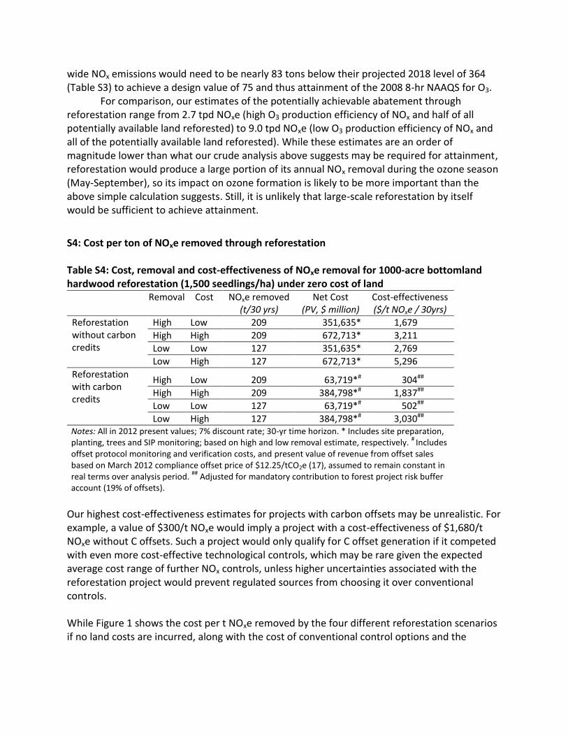
S4: Cost per ton of NOxe removed through reforestation Table S4: Cost, removal and cost-effectiveness of NOxe removal for 1000-acre bottomland hardwood reforestation (1,500 seedlings/ha) under zero cost of land

Removal Cost NOxe removed (t/30 yrs)

Net Cost (PV, $ million)

Cost-effectiveness ($/t NOxe / 30yrs)

Reforestation without carbon credits

High Low 209 351,635* 1,679

High High 209 672,713* 3,211

Low Low 127 351,635* 2,769

Low High 127 672,713* 5,296

Reforestation with carbon credits

High Low 209 63,719*# 304##

High High 209 384,798*# 1,837##

Low Low 127 63,719*# 502##

Low High 127 384,798*# 3,030## Notes: All in 2012 present values; 7% discount rate; 30-yr time horizon. * Includes site preparation, planting, trees and SIP monitoring; based on high and low removal estimate, respectively.

# Includes

offset protocol monitoring and verification costs, and present value of revenue from offset sales based on March 2012 compliance offset price of $12.25/tCO2e (17), assumed to remain constant in real terms over analysis period.

## Adjusted for mandatory contribution to forest project risk buffer

account (19% of offsets).

Our highest cost-effectiveness estimates for projects with carbon offsets may be unrealistic. For example, a value of $300/t NOxe would imply a project with a cost-effectiveness of $1,680/t NOxe without C offsets. Such a project would only qualify for C offset generation if it competed with even more cost-effective technological controls, which may be rare given the expected average cost range of further NOx controls, unless higher uncertainties associated with the reforestation project would prevent regulated sources from choosing it over conventional controls. While Figure 1 shows the cost per t NOxe removed by the four different reforestation scenarios if no land costs are incurred, along with the cost of conventional control options and the

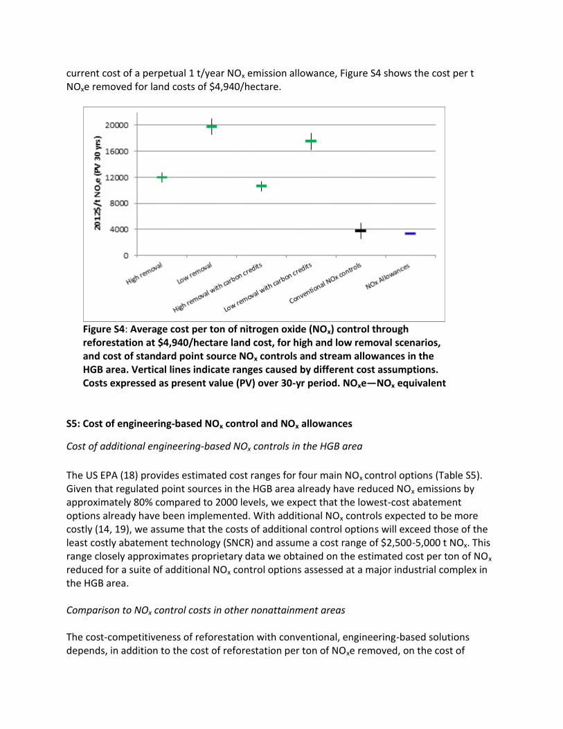
current cost of a perpetual 1 t/year NOx emission allowance, Figure S4 shows the cost per t NOxe removed for land costs of $4,940/hectare.

Figure S4: Average cost per ton of nitrogen oxide (NOx) control through reforestation at $4,940/hectare land cost, for high and low removal scenarios, and cost of standard point source NOx controls and stream allowances in the HGB area. Vertical lines indicate ranges caused by different cost assumptions. Costs expressed as present value (PV) over 30-yr period. NOxe—NOx equivalent

S5: Cost of engineering-based NOx control and NOx allowances

Cost of additional engineering-based NOx controls in the HGB area

The US EPA (18) provides estimated cost ranges for four main NOx control options (Table S5). Given that regulated point sources in the HGB area already have reduced NOx emissions by approximately 80% compared to 2000 levels, we expect that the lowest-cost abatement options already have been implemented. With additional NOx controls expected to be more costly (14, 19), we assume that the costs of additional control options will exceed those of the least costly abatement technology (SNCR) and assume a cost range of $2,500-5,000 t NOx. This range closely approximates proprietary data we obtained on the estimated cost per ton of NOx reduced for a suite of additional NOx control options assessed at a major industrial complex in the HGB area. Comparison to NOx control costs in other nonattainment areas The cost-competitiveness of reforestation with conventional, engineering-based solutions depends, in addition to the cost of reforestation per ton of NOxe removed, on the cost of

engineering-based NOx controls. A crucial question for the generalizability of our case study findings therefore is whether the costs of those engineered controls in other nonattainment areas are similar to what they are in our case study area. The range and average of the point source NOx control costs in a given area are a function of many factors. These include the industrial composition of the area’s point sources, which may affect the composition of NOx-emitting processes and thus control options and costs; the share of new and old sources, which affects the shares of point sources subject to the Reasonably Available Control Technology standard (RACT—applicable to sources already in existence when a SIP was first approved) and the Lowest Achievable Emission Rate standard (LAER—the most stringent category of emission control, applicable to new sources in non-attainment areas and to major modifications of existing sources), respectively; the stringency of RACT, that is, what is defined in the area as “reasonable” in terms of costs per t NOx reduced; the current state-of-the-art of NOx control, which defines what is considered LAER; and the degree of severity of nonattainment, which affects the annual emission quantity used to define a stationary source as a “point source”—the higher the nonattainment classification, the lower the emission quantity at which a stationary source becomes classified as a point source and thus is subject to point source regulations.1

Extensive literature searches revealed that information on the average NOx control costs for point sources, or on the range of point source NOx control costs, is not available for nonattainment areas overall. Individual analyses for specific sources can be found, but because of the large number and variety (types and specific characteristics) of NOx point sources in any nonattainment area, it is impossible to generalize from these individual data points to an area as a whole. For our HGB-area case study, we used an assumed control cost range ($2,500-$5,000 per ton of NOx reduced; see S5 above) that matches proprietary and confidential information we obtained on the next suite of NOx control projects that have been identified for implementation at a very large industrial complex in the HGB area that contains a large number and variety of processes subject to NOx control. This chosen range falls within the $1,600-$6,600 average costs per ton of NOx abatement reported for available NOx control approaches commonly employed by point sources (Table S5). Lacking information on averages or ranges of attainment area-specific NOx control costs, estimates of average NOx control costs for other nonattainment areas might be constructed by identifying the total NOx abatement achieved in an area and combining that information with an estimated marginal NOx control cost curve for large stationary sources. This approach is problematic for two reasons: To our knowledge, the only published abatement cost curve for large stationary sources as a group is for large electric power plants (19). Thus, one would need to assume that the abatement cost curve of other point sources is similar to that of power plants. This may be problematic, because for a given technology, control costs vary by process size, and they do so non-linearly (18). Second, no centralized database exists that contains

1 This threshold quantity ranges from 25 tons per year (severe nonattainment) to 100 tons per year (marginal

nonattainment) of ozone precursor emission potential.

information on point source—or area-wide—NOx emission reductions for US O3 non-attainment areas. Rather, that information is spread out over hundreds of technical reports and thus is not easily compiled. Finally, the representativeness of Houston-area NOx controls for US nonattainment areas may be assessed by comparing the stringency of Houston-area point source NOx controls with that found in other nonattainment areas. If control stringency in other nonattainment areas is comparable to that found in the HGB area, then one could argue that Houston-area point source control costs per t NOx removed might be reasonably representative of such costs in other nonattainment areas. This is the approach we take here. Point sources (electric generating units and other large stationary sources combined) in the Houston nonattainment area are estimated to have reduced NOx emissions by an area-wide average 80% since the year 2000 (15). Thus, Houston clearly is fairly well along the NOx abatement curve, at least as far as point sources are concerned. However, the same is increasingly true for large portions of the US. For example, under the 2005 Clean Air Interstate Rule (CAIR) and its successor, the 2011 Cross-State Air Pollution Rule (CSAPR), electric generating units in 27 eastern states and the District of Columbia are required to install controls that by 2020 will reduce their NOx emissions by an estimated 61% from 2003 levels (at which time a large proportion of those sources already where subject to NOx control through ozone SIPs) (CAIR; http://www.epa.gov/cair/basic.html; see our discussion below).2 Likewise, EPA assumes that by 2020, other point sources (i.e., not electric generating units) as well as area sources in 189 counties in Texas (not counting the 8-county Houston-Galveston-Brazoria nonattainment area we cover in our study), California, Illinois, Indiana and Michigan that are

2 CSAPR was vacated by the US Court of Appeals for the District of Columbia in August of 2012 (20). The court cited

two reasons for that decision. First, it argued that as currently designed, the rule exceeded EPA’s statutory authority. That authority stems from the “Good Neighbor Rule” in the Clean Air Act and Amendments, which allows EPA to require an upwind state to reduce its “own significant contribution” to downwind states’ nonattainment areas. The court held that CSAPR, as currently designed, exceeded statutory limitations by effectively imposing emission reductions on some states that were exceeding their “own significant contribution.” As currently written, CSAPR employs a cap-and-trade mechanism to allocate the mandated emission reductions across the 27 states and DC. This mechanism was chosen to minimize overall abatement costs across the CSAPR states. It is also the reason why some states might, under CSAPR, end up reducing their emissions to below what might be judged their “own significant contribution." Thus, EPA could conceivably replace this market-based mechanism for the whole CSAPR area with individual ones for each state to address the appeals court’s concern. That would likely result in higher abatement costs in some states subject to the rule, and lower costs in others than would be the case under the rule as currently written. Overall, abolishing the market-based allocation of emission reductions, or replacing it with state-by-state cap-and-trade markets, would increase the average abatement cost per ton of NOx across the CSAPR area.

The second reason the appeals court cited for striking down CSAPR was that, in the court’s view, the Clean Air Act granted states the initial opportunity to implement emission reductions required by EPA. The court held that by imposing Federal Implementation Plans under CSAPR at the outset, EPA departed from its “consistent prior approach” of implementing the Good Neighbor provision and violated the Act. The issue is now before the US Supreme Court, which in June 2013 agreed to review the DC Circuit Court’s decision. It is expected that, if required, EPA will change CSAPR to adapt to the courts’ decisions. In the meantime, EPA is required to implement the earlier CAIR rule.

subject to CSAPR will need to deploy the sector-specific NOx control technologies currently deployed in the HGB-area to achieve compliance with current NAAQS.3 This includes all counties in California, Illinois and Michigan classified as nonattainment under the 2008 O3 standard in 2013. Notably, the EPA has pursued more stringent standards for O3 (22) and in December 2012 tightened its PM2.5 standard (23; NOx is an important contributor to ambient concentrations of PM2.5). Under the proposed more stringent ozone standard, the area in which these and more stringent control measures would be necessary to achieve compliance with ozone standards would more than double.4

Thus, the stringency of point source NOx controls found in many other non-attainment area is expected to already—and increasingly —be similar to that found in the Houston area.

Even if ozone standards are not tightened further, the persistent failure to attain current ozone NAAQS already is leading some states to increase abatement requirements for sources by revising their definitions of what constitutes RACT for NOx—the level of NOx control that all existing major NOx emission sources in nonattainment areas must achieve. This raises average abatement costs. For example, New York did so in 2010 (24; source compliance deadline 07/31/2012). As a result, New York State now uses a RACT cost threshold (the threshold up to which a source is required to install RACT) of $5,000 per t NOx reduced (2012 dollars; 25), over 20% higher (in constant dollars) than our assumed mean cost for conventional controls ($3,750 in 2012 dollars; see Fig. 1). Likewise, California’s San Joaquin Valley Air Pollution Control District in 2008 raised its Best Available Control Technology (BACT; the control level required by new sources or major modifications of existing sources in attainment areas) cost threshold from $9,700 to $24,500/t NOx reduced (26).

There is another, more important reason why our estimates of the cost of NOx reductions for engineering estimates are unlikely to fall outside of the range of NOx control cost with which reforestation would compete elsewhere. Our case study, site-level-based cost estimates are for existing major sources in a nonattainment area, which are required to install RACT. However, all new major sources in such areas, and all major modifications to existing sources, must install LAER technology, the most stringent control standard under the Clean Air Act. And even in attainment areas, all new sources must install BACT, which also is more stringent than RACT. Both BACT and LAER are more costly than RACT.5, 6 With the average cost per ton of additional NOx reductions in nonattainment areas being the weighted average of control costs at existing

3 See Table 3.1 and Figure 3.1 in (21)

4 See Fig. 3.5 in (21).

5 For example, in California’s San Joaquin Valley Air Pollution Control District, the BACT threshold for major point

sources currently is $24,500/t NOx reduced, while for RACT it is $8,000-10,000 /t depending on source. In six other major California air quality management districts (San Diego, Sacramento, Bay Area, South Coast, Yolo-Solano and Ventura), the BACT thresholds range from $13,200-24,500 per t NOx reduced (26, 27). 6 It is thus not surprising that our case study site-specific range of estimated conventional NOx reduction costs

($2,500-$5,000/ ton NOx reduced) is contained within the range of NOx control costs for major stationary sources described in Table S5. The control technologies described in Table S5 cover a range of NOx removal efficiencies. The technologies that achieve the highest removal are generally the costliest, all things equal (process type and size, retrofit vs. new process), and are generally only required for new sources or major modifications, while our case study cost estimates are for exiting sources.

sources (subject to RACT) and new sources (subject to the much more stringent LAER standard), that average cost will be higher than the average cost for RACT NOx control at existing sources, which is what our case study cost estimates are based on. It is those additional NOx controls that reforestation projects would compete with because, under current EPA policy guidance (28), reforestation could not be used to replace emission controls already written into a SIP. Those additional controls would, by definition, come from more stringent control mandates for existing sources (in cases where existing SIP efforts are insufficient to achieve attainment of NAAQS and result in updated classification of RACT technology such as in the case of New York discussed above) and from state-of-the-art controls (LAER) on new sources or major modifications of existing sources. As already discussed, those additional controls are likely to be costlier per t NOx reduced than the controls analyzed in our case study, both due to the tighter control requirements of the applicable control level (LAER and BACT vs. RACT) and because of the rising technology and cost thresholds that define a given control standard (RACT, BACT and LAER).

Therefore, it is reasonable to assume that in many other nonattainment areas, reforestation would compete against engineering-based NOx controls whose cost per t NOx reduced will be similar or higher than those used in our case study.

Table S5: Cost effectiveness estimates of main NOx control options

Control option 2012$/t NOx Low High Avg.

LNB (Low NOx burner) 382 6,837 3,609 LNB+FGR (Flue gas recirculation) 1,034 12,132 6,583 SNCR (Selective non-catalytic reduction) 1,113 2,067 1,590 SCR 795 4,452 2,624

Source: (18), adjusted to 2012$ using US Consumer Price Index.

Cost of NOx allowances The TCEQ March 1, 2013 report on NOx allowance trades in the HGB area (29) lists a total of 28 non-zero price trades of NOx “stream” (perpetual for life of the HGB-area Mass Emissions Cap and Trade [MECT] program)) allowances between 1 January 2012 and 29 February 2013, with an average weighted price of $92,187/t NOx. One NOx stream allowance entitles its holder to annual emissions of 1 t NOx. Given the projected continued, strong economic growth of the HGB area (30) as well as of the industrial and utility sectors (31), and especially the large growth in the shale gas production sector and ancillary industries, we expect that demand for NOx allowances will increase during our 30-yr modeling period. In addition, possible NAAQS O3 standard revisions considered by the U.S. EPA could curtail the total number of MECT NOx allocations, increasing the scarcity of allowances. Under the fixed or possibly declining overall HGB area point source NOx emission cap, we expect that increased demand for NOx allowances will lead to an increase in allowance prices compared to those observed in the recent past. We use a price of $100,000/t NOx as the average allowance price―consistent with the planning

price used by The Dow Chemical Company. Over a 30-yr period, one NOx stream allowance entitles its holder to emissions of a total of 30 t NOx, thus resulting in the average price of $3,333/t NOx used in our analysis. S6: VOC emission modeling and estimation of the VOC balance of the project

VOC emission potential of planted species

Guenther et al. (32) proposed a classification system for normalized (basal rate of midsummer fully exposed foliage) leaf-level isoprene emission rates that consists of four emission ranges (expressed in μg Cg-1 h-1): (1) negligible: ~0.1; (2) low: 14 ± 7; (3) moderate: 35 ± 17.5; and (4) high: 70 ± 35. Geron et al. (33) found a clear breakdown of isoprene emissions for broadleaf species into very low (<1 μg Cg-1 h-1) and high (100+/-50 μg Cg-1 h-1) emitters, and noted that the variability in emission factors is likely large enough to obscure most interspecies differences in isoprene emission factors within existing databases.

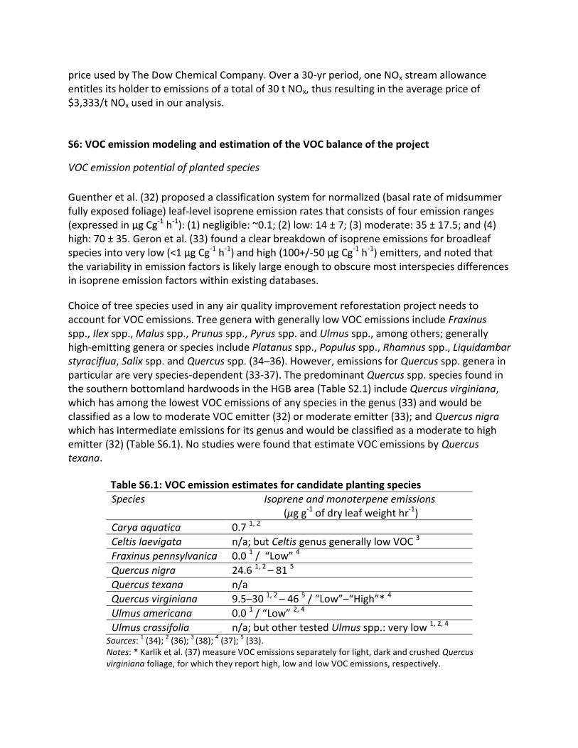
Choice of tree species used in any air quality improvement reforestation project needs to account for VOC emissions. Tree genera with generally low VOC emissions include Fraxinus spp., Ilex spp., Malus spp., Prunus spp., Pyrus spp. and Ulmus spp., among others; generally high-emitting genera or species include Platanus spp., Populus spp., Rhamnus spp., Liquidambar styraciflua, Salix spp. and Quercus spp. (34–36). However, emissions for Quercus spp. genera in particular are very species-dependent (33-37). The predominant Quercus spp. species found in the southern bottomland hardwoods in the HGB area (Table S2.1) include Quercus virginiana, which has among the lowest VOC emissions of any species in the genus (33) and would be classified as a low to moderate VOC emitter (32) or moderate emitter (33); and Quercus nigra which has intermediate emissions for its genus and would be classified as a moderate to high emitter (32) (Table S6.1). No studies were found that estimate VOC emissions by Quercus texana.

Table S6.1: VOC emission estimates for candidate planting species

Species Isoprene and monoterpene emissions (μg g-1 of dry leaf weight hr-1)

Carya aquatica 0.7 1, 2

Celtis laevigata n/a; but Celtis genus generally low VOC 3

Fraxinus pennsylvanica 0.0 1 / “Low” 4

Quercus nigra 24.6 1, 2 – 81 5

Quercus texana n/a

Quercus virginiana 9.5–30 1, 2 – 46 5 / “Low”–“High”* 4

Ulmus americana 0.0 1 / “Low” 2, 4

Ulmus crassifolia n/a; but other tested Ulmus spp.: very low 1, 2, 4 Sources:

1 (34);

2 (36);

3 (38);

4 (37);

5 (33).

Notes: * Karlik et al. (37) measure VOC emissions separately for light, dark and crushed Quercus virginiana foliage, for which they report high, low and low VOC emissions, respectively.

The other species identified as candidates for planting in the bottomland reforestation project (Table S2.1) are all classified as low or very low VOC emitters except for Celtis laevigata, for which we were unable to find VOC emission estimates (Table S6.1). The Celtis genus, however, is characterized by low VOC emissions (38).

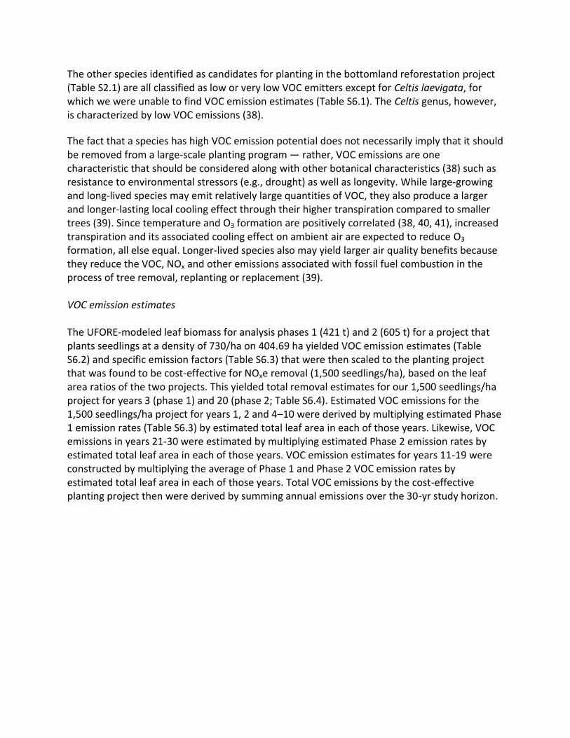
The fact that a species has high VOC emission potential does not necessarily imply that it should be removed from a large-scale planting program ― rather, VOC emissions are one characteristic that should be considered along with other botanical characteristics (38) such as resistance to environmental stressors (e.g., drought) as well as longevity. While large-growing and long-lived species may emit relatively large quantities of VOC, they also produce a larger and longer-lasting local cooling effect through their higher transpiration compared to smaller trees (39). Since temperature and O3 formation are positively correlated (38, 40, 41), increased transpiration and its associated cooling effect on ambient air are expected to reduce O3 formation, all else equal. Longer-lived species also may yield larger air quality benefits because they reduce the VOC, NOx and other emissions associated with fossil fuel combustion in the process of tree removal, replanting or replacement (39). VOC emission estimates The UFORE-modeled leaf biomass for analysis phases 1 (421 t) and 2 (605 t) for a project that plants seedlings at a density of 730/ha on 404.69 ha yielded VOC emission estimates (Table S6.2) and specific emission factors (Table S6.3) that were then scaled to the planting project that was found to be cost-effective for NOxe removal (1,500 seedlings/ha), based on the leaf area ratios of the two projects. This yielded total removal estimates for our 1,500 seedlings/ha project for years 3 (phase 1) and 20 (phase 2; Table S6.4). Estimated VOC emissions for the 1,500 seedlings/ha project for years 1, 2 and 4–10 were derived by multiplying estimated Phase 1 emission rates (Table S6.3) by estimated total leaf area in each of those years. Likewise, VOC emissions in years 21-30 were estimated by multiplying estimated Phase 2 emission rates by estimated total leaf area in each of those years. VOC emission estimates for years 11-19 were constructed by multiplying the average of Phase 1 and Phase 2 VOC emission rates by estimated total leaf area in each of those years. Total VOC emissions by the cost-effective planting project then were derived by summing annual emissions over the 30-yr study horizon.

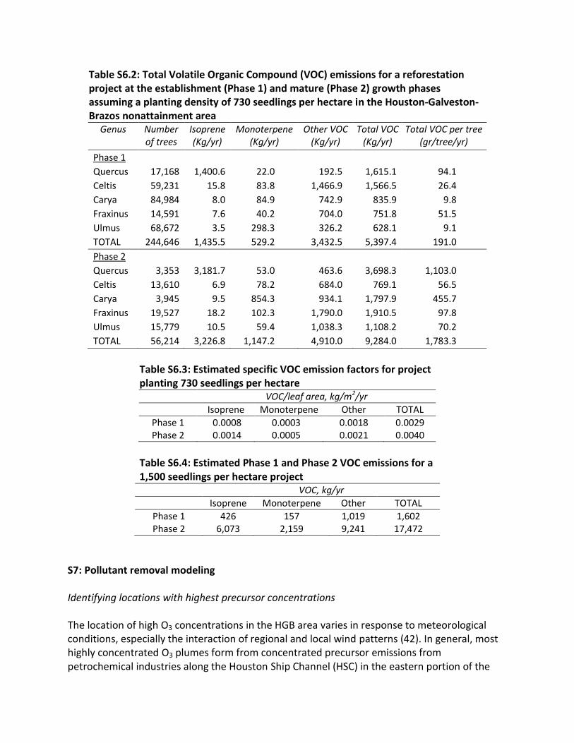
Table S6.2: Total Volatile Organic Compound (VOC) emissions for a reforestation project at the establishment (Phase 1) and mature (Phase 2) growth phases assuming a planting density of 730 seedlings per hectare in the Houston-Galveston-Brazos nonattainment area

Genus Number of trees

Isoprene (Kg/yr)

Monoterpene (Kg/yr)

Other VOC (Kg/yr)

Total VOC (Kg/yr)

Total VOC per tree (gr/tree/yr)

Phase 1

Quercus 17,168 1,400.6 22.0 192.5 1,615.1 94.1

Celtis 59,231 15.8 83.8 1,466.9 1,566.5 26.4

Carya 84,984 8.0 84.9 742.9 835.9 9.8

Fraxinus 14,591 7.6 40.2 704.0 751.8 51.5

Ulmus 68,672 3.5 298.3 326.2 628.1 9.1

TOTAL 244,646 1,435.5 529.2 3,432.5 5,397.4 191.0

Phase 2

Quercus 3,353 3,181.7 53.0 463.6 3,698.3 1,103.0

Celtis 13,610 6.9 78.2 684.0 769.1 56.5

Carya 3,945 9.5 854.3 934.1 1,797.9 455.7

Fraxinus 19,527 18.2 102.3 1,790.0 1,910.5 97.8

Ulmus 15,779 10.5 59.4 1,038.3 1,108.2 70.2

TOTAL 56,214 3,226.8 1,147.2 4,910.0 9,284.0 1,783.3

Table S6.3: Estimated specific VOC emission factors for project planting 730 seedlings per hectare VOC/leaf area, kg/m2/yr

Isoprene Monoterpene Other TOTAL

Phase 1 0.0008 0.0003 0.0018 0.0029 Phase 2 0.0014 0.0005 0.0021 0.0040

Table S6.4: Estimated Phase 1 and Phase 2 VOC emissions for a 1,500 seedlings per hectare project VOC, kg/yr

Isoprene Monoterpene Other TOTAL

Phase 1 426 157 1,019 1,602 Phase 2 6,073 2,159 9,241 17,472

S7: Pollutant removal modeling Identifying locations with highest precursor concentrations The location of high O3 concentrations in the HGB area varies in response to meteorological conditions, especially the interaction of regional and local wind patterns (42). In general, most highly concentrated O3 plumes form from concentrated precursor emissions from petrochemical industries along the Houston Ship Channel (HSC) in the eastern portion of the

Houston metro area and then move through the metro area depending on wind direction (43). Ozone often reaches its highest measured area-wide concentrations in southwestern or western Harris County, and high concentrations are also often observed in northern Brazoria County (p. 5-5 in [44]; Fig S7.1).7 However, if monitor density in Brazoria and Fort Bend Counties were greater, maximum HGB area-wide concentrations might be observed occasionally in those counties rather than Harris County (44).

Figure S7.1: Ozone design values (fourth highest 8-hour average ozone concentration observed in the year) in the HGB area for selected years (16)

Maximum removal of NO2 by tree canopy is achieved in areas directly downwind of major emission sources, where canopy can intercept highly concentrated plumes of NOx before they become diluted by atmospheric mixing processes. Given the density of the current net of continuous air monitoring stations (CAMS) in the HGB area, it is likely that concentrated NOx plumes generally will have been diluted by the time they reach a CAMS. Thus, combining information on NOx emissions and prevailing winds would be the preferred approach for identifying optimal reforestation sites for purposes of NOx removal, rather than using ambient concentrations recorded by air quality monitors.

7 Generally, the highest ozone values occur between late May and mid-September, with the highest number of

exceedance days between late July and mid-September (fig. 2-8 in [44]).

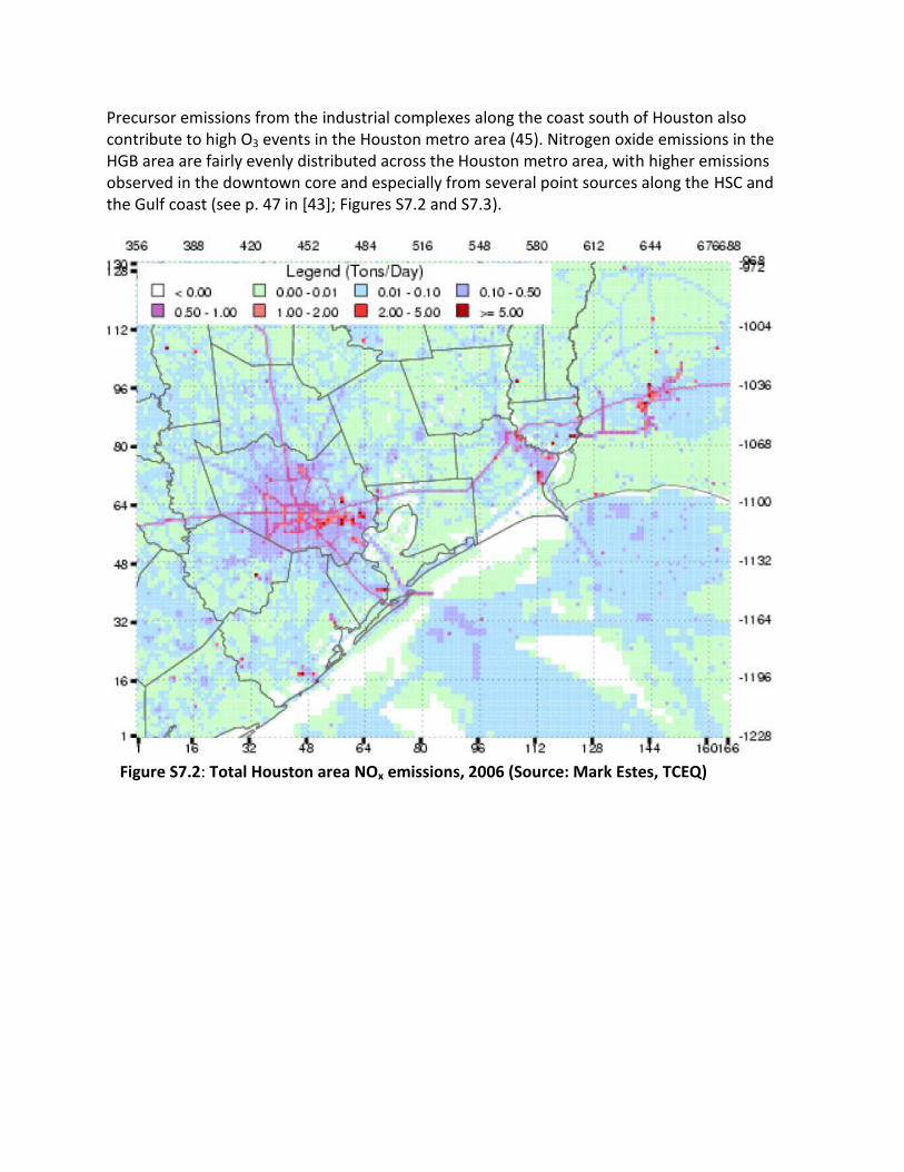
Precursor emissions from the industrial complexes along the coast south of Houston also contribute to high O3 events in the Houston metro area (45). Nitrogen oxide emissions in the HGB area are fairly evenly distributed across the Houston metro area, with higher emissions observed in the downtown core and especially from several point sources along the HSC and the Gulf coast (see p. 47 in [43]; Figures S7.2 and S7.3).

Figure S7.2: Total Houston area NOx emissions, 2006 (Source: Mark Estes, TCEQ)

Figure S7.3: Nitrogen oxide (NOx) point source emissions in the Houston area, 2006 (46)

Information on the prevailing winds in the HGB area can help determine where reforested stands would be most likely to intercept air masses with high O3 and NOx levels. The HGB area is characterized by winds that typically rotate continuously throughout the day. In the morning, winds blow from the northeast; by noon, from the east; in the afternoon, from southeast; after sunset, from south and west, and by midnight, from the southwest (14). This pattern is also typical of days on which eight-hour O3 levels in the HGB area exceed the NAAQS (44). Three main wind patterns have been identified that generate O3 episodes: Flow reversals; typical veering; and steady flow, accounting for 53%, 32% and 15%, respectively, of all classified episode days during 2003-2006 (Table 5-4 in [44]). During flow reversal days, initially light winds with a westerly component are replaced by a

period of stagnation allowing emission build-up in industrial and urban areas, and then a reversal of wind flow to the east or southeast due to a slow intrusion of the bay breeze from the east, and finally to the southern peri-urban areas due to the arrival of the Gulf breeze (p. 5-8 in [44]). This results in pollutants moving first south towards Galveston Bay and the Gulf and then returning towards the metro area where they mix with fresh precursor emissions. This suggests that for maximum O3 removal, reforestation projects should be sited south of the industrial sources along the HSC or north of the petrochemical complexes along the coast to the south of the metro area.

A typical veering episode day begins with winds from the northeast that gradually shift clockwise to the east, southeast, and south. These winds slowly carry emissions from industrial and urban areas of the HGB area during early morning hours (0000-0800) into southeast Harris County. By 2000 CDT, winds have shifted from east northeast to east to southeast to south southeast, carrying industrial plumes into south Houston, and then into west Houston (44). Highest O3 removal by the forest canopy on typical veering days would be achieved within an area of approximately triangular shape that extends from the beginning of the HSC westward into northern Brazoria and Fort Bend counties in the south and the western portion of Harris County.

Steady Flow episodes are characterized by winds that blow from essentially the same direction for most of the day with only minor fluctuations (p. 5-15 in [44]). The most common winds during steady flow episodes that cause O3 events usually have northerly and easterly components, although winds with strong westerly or southerly components on rare occasions also cause O3 events (44). Steady flow events generally producer lower O3 levels than flow reversal or veering days and account for a much smaller share of O3 exceedances (Table 5-4 in [44]). With most steady flow O3 events characterized by northerly or easterly winds, tree canopy south or southwest of the main emission sources along the HSC would be likely to lead to highest O3 removal rates. During the rarer steady flow events characterized by southerly or westerly winds, tree canopy north of the major coastal point sources likely would produce the highest removal. The goal of maximizing O3 removal thus could be pursued by reforestation within fairly broad geographic areas. This contrasts with the fairly small areas just downwind of major point sources in which trees would deliver maximum NOx removal. Considering the frequency distribution of the diurnally shifting winds (47), reforested stands located just downwind from major point sources in southerly, westerly or northerly direction would be expected to remove the most NOx.

The combined removal of O3 and NOx would be highest just downwind in southerly, westerly or northerly direction of major point sources located along the HSC and the Gulf coast. Ambient pollutant concentrations and meteorological conditions used in UFORE modeling Mark Estes, Senior Air Quality Scientist with TCEQ’s Air Quality Division suggested 2009 as a

representative year for meteorological conditions in the HGB area. Hourly meteorological and pollution concentration data were obtained from the monitoring sites (see Methods) for the period January 1 to December 31, 2009. Table S7.1 summarizes these hourly data as monthly averages. We assumed that 2009 conditions (Table S7.1) remain constant during our 30-yr modeling horizon.

Table S7.1: Monthly averages of pollutant concentrations (NO2, O3), temperature, wind speed, tree crown water transpiration (transp.) and pollutant flux

Month NO2 (ppm)

O3 (ppm)

Temp. (K) Wind speed (m/sec)

Transp. g hr-1 m-2

Flux g m-2 hr-1

January 0.0085448 0.0204589 285.7 3.0 0 0.00005 February 0.0079848 0.0200520 289.5 3.8 7.4 0.00011 March 0.0085448 0.0204589 290.1 3.6 27.6 0.00028 April 0.0086778 0.0199546 293.6 4.2 50.3 0.00032 May 0.0085448 0.0204589 298.2 3.0 69.2 0.00033 June 0.0086778 0.0199546 300.9 2.4 79.4 0.0003 July 0.0085448 0.0204589 302.0 2.2 69.7 0.00028 August 0.0085448 0.0204589 302.0 1.7 66.1 0.00027 September 0.0086778 0.0199546 298.9 2.0 49 0.00029 October 0.0085448 0.0204589 295.3 3.2 38.4 0.00026 November 0.0086778 0.0199546 290.1 2.3 5.2 0.00007 December 0.0085448 0.0204589 284.9 3.3 0 0.00004

The Manvel Croix Park monitoring station is the one closest to our reforestation site and was identified by TCEQ air quality modelers as the preferred site to use in our analysis because of prevailing winds and expected very similar O3 and NO2 concentrations. Consideration of climate change impacts on pollutant concentrations Climate change is expected to increase average summertime temperatures in southern Texas (48) and may lead to increased O3 formation (49–52). In fact, Jiang et al. (53) estimate that climate change and land use change will be of roughly equal importance in driving future changes in O3 formation in the Houston area. However, due to modeling uncertainties, the U.S. EPA currently does not require―and TCEQ does not include―modeling of climate change impacts on future O3 concentrations in SIPs. Therefore we assume that O3 concentrations and meteorological parameters will remain constant over the 30-yr analysis period. Estimation of the VOC balance of the project We use Carter’s (54) Maximum Incremental Reactivity (MIR) scales (gm O3/gm VOC) for isoprene and monoterpenes (10.61 and 4.04, respectively) and derive MIR scale reactivities for other VOCs (OVOCs) as a group (not given in [54]) by multiplying isoprene MIR reactivity values by the ratio of the estimated daytime chemical lifetimes of isoprene (3 hrs) and OVOCs (>24

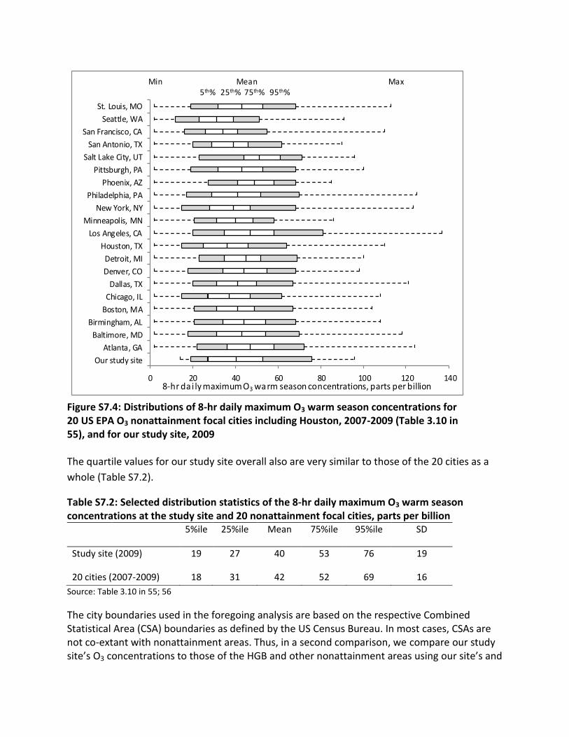
hrs―we use 24 hrs; 36). We scale reactivities using atmospheric lifetimes because lifetime is a good indicator of reactivity (38). Comparison of Houston-area O3 and NO2 concentrations with those of other US nonattainment areas Ozone concentrations. To assess how the O3 concentrations used in our modeling compare to those found in other areas, we first compare our study site concentrations (taken from the Manvel Croix Park US EPA Air Quality Site, AQS ID #480391004) to those of Houston and 19 other large cities in nonattainment areas that the US EPA has selected to investigate the urban-scale variability of O3 concentrations. Figure S7.4 shows the distributions (minimum, mean, maximum and the 5th, 25th, 75th and 95th percentile values) of the 8-hr daily maximum O3 concentrations for the 20 cities during the 2007-2009 warm seasons (May-September), and for our study site for 2009, the year used in our modeling. Figure S7.4 shows that the range of O3 concentrations observed at our study site is smaller than that of the 20 cities. This is likely due to the fact that the data for our site are from only a single year while those for the 20 cities cover three years. The mean 8-hr daily maximum O3 concentration at our site, 40 ppb, is slightly above Houston’s (36 ppb) but slightly below the mean of the other cities (42 ppb).

0 20 40 60 80 100 120 140

Our study site

Atlanta, GA

Baltimore, MD

Birmingham, AL

Boston, MA

Chicago, IL

Dallas, TX

Denver, CO

Detroit, MI

Houston, TX

Los Angeles, CA

Minneapolis, MN

New York, NY

Philadelphia, PA

Phoenix, AZ

Pittsburgh, PA

Salt Lake City, UT

San Antonio, TX

San Francisco, CA

Seattle, WA

St. Louis, MO

8-hr da i ly maximum O3 warm season concentrations, parts per billion

Min Mean Max 5th% 25th% 75th% 95th%

Figure S7.4: Distributions of 8-hr daily maximum O3 warm season concentrations for 20 US EPA O3 nonattainment focal cities including Houston, 2007-2009 (Table 3.10 in 55), and for our study site, 2009 The quartile values for our study site overall also are very similar to those of the 20 cities as a

whole (Table S7.2).

Table S7.2: Selected distribution statistics of the 8-hr daily maximum O3 warm season concentrations at the study site and 20 nonattainment focal cities, parts per billion

5%ile 25%ile Mean 75%ile 95%ile SD

Study site (2009) 19 27 40 53 76 19

20 cities (2007-2009) 18 31 42 52 69 16

Source: Table 3.10 in 55; 56

The city boundaries used in the foregoing analysis are based on the respective Combined Statistical Area (CSA) boundaries as defined by the US Census Bureau. In most cases, CSAs are not co-extant with nonattainment areas. Thus, in a second comparison, we compare our study site’s O3 concentrations to those of the HGB and other nonattainment areas using our site’s and

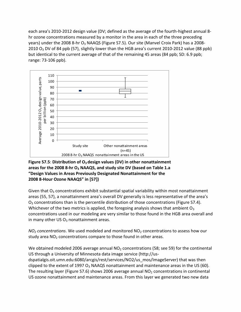
each area’s 2010-2012 design value (DV; defined as the average of the fourth-highest annual 8-hr ozone concentrations measured by a monitor in the area in each of the three preceding years) under the 2008 8-hr O3 NAAQS (Figure S7.5). Our site (Manvel Croix Park) has a 2008-2010 O3 DV of 84 ppb (57), slightly lower than the HGB area’s current 2010-2012 value (88 ppb) but identical to the current average of that of the remaining 45 areas (84 ppb; SD: 6.9 ppb; range: 73-106 ppb).

0. 1

0

10

20

30

40

50

60

70

80

90

100

110

Study site Other nonattainment areas(n=45)

Ave

rage

20

10

-20

12

O3

des

ign

va

lue,

pa

rts

per

bil

lio

n (p

pb

)

2008 8-hr O3 NAAQS nonattainment areas in the US

Figure S7.5: Distribution of O3 design values (DV) in other nonattainment areas for the 2008 8-hr O3 NAAQS, and study site DV (based on Table 1.a “Design Values in Areas Previously Designated Nonattainment for the 2008 8-Hour Ozone NAAQS” in [57]) Given that O3 concentrations exhibit substantial spatial variability within most nonattainment areas (55, 57), a nonattainment area’s overall DV generally is less representative of the area’s O3 concentrations than is the percentile distribution of those concentrations (Figure S7.4). Whichever of the two metrics is applied, the foregoing analysis shows that ambient O3 concentrations used in our modeling are very similar to those found in the HGB area overall and in many other US O3 nonattainment areas.

NO2 concentrations. We used modeled and monitored NO2 concentrations to assess how our study area NO2 concentrations compare to those found in other areas. We obtained modeled 2006 average annual NO2 concentrations (58; see 59) for the continental US through a University of Minnesota data image service (http://us-dspatialgis.oit.umn.edu:6080/arcgis/rest/services/NO2/us_mos/ImageServer) that was then clipped to the extent of 1997 O3 NAAQS nonattainment and maintenance areas in the US (60). The resulting layer (Figure S7.6) shows 2006 average annual NO2 concentrations in continental US ozone nonattainment and maintenance areas. From this layer we generated two new data

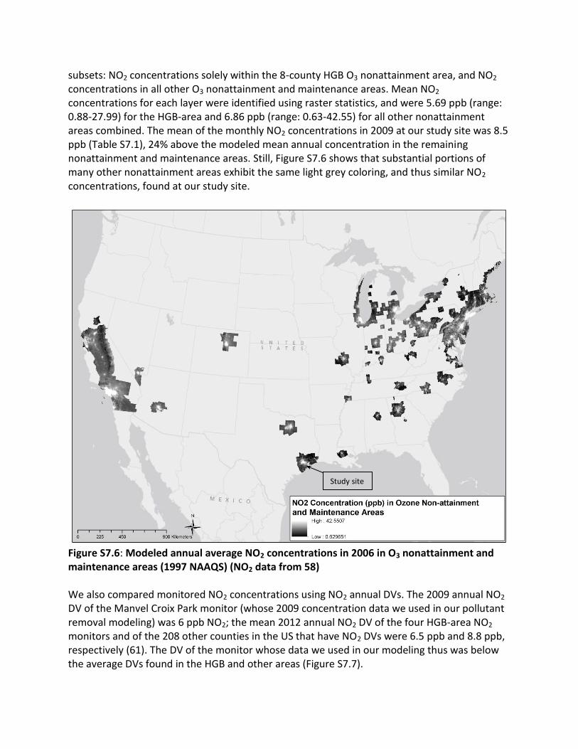
subsets: NO2 concentrations solely within the 8-county HGB O3 nonattainment area, and NO2 concentrations in all other O3 nonattainment and maintenance areas. Mean NO2 concentrations for each layer were identified using raster statistics, and were 5.69 ppb (range: 0.88-27.99) for the HGB-area and 6.86 ppb (range: 0.63-42.55) for all other nonattainment areas combined. The mean of the monthly NO2 concentrations in 2009 at our study site was 8.5 ppb (Table S7.1), 24% above the modeled mean annual concentration in the remaining nonattainment and maintenance areas. Still, Figure S7.6 shows that substantial portions of many other nonattainment areas exhibit the same light grey coloring, and thus similar NO2 concentrations, found at our study site.

Figure S7.6: Modeled annual average NO2 concentrations in 2006 in O3 nonattainment and maintenance areas (1997 NAAQS) (NO2 data from 58) We also compared monitored NO2 concentrations using NO2 annual DVs. The 2009 annual NO2 DV of the Manvel Croix Park monitor (whose 2009 concentration data we used in our pollutant removal modeling) was 6 ppb NO2; the mean 2012 annual NO2 DV of the four HGB-area NO2 monitors and of the 208 other counties in the US that have NO2 DVs were 6.5 ppb and 8.8 ppb, respectively (61). The DV of the monitor whose data we used in our modeling thus was below the average DVs found in the HGB and other areas (Figure S7.7).

Study site

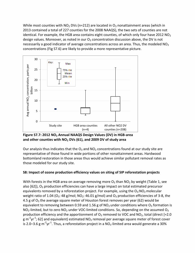
While most counties with NO2 DVs (n=212) are located in O3 nonattainment areas (which in 2013 contained a total of 227 counties for the 2008 NAAQS), the two sets of counties are not identical. For example, the HGB area contains eight counties, of which only four have 2012 NO2 design values. Moreover, as noted in our O3 concentration discussion above, the DV is not necessarily a good indicator of average concentrations across an area. Thus, the modeled NO2 concentrations (Fig S7.6) are likely to provide a more representative picture.

Figure S7.7: 2012 NO2 Annual NAAQS Design Values (DV) in HGB-area and other counties with NO2 DVs (61), and 2009 DV of study area Our analysis thus indicates that the O3 and NO2 concentrations found at our study site are representative of those found in wide portions of other nonattainment areas. Hardwood bottomland restoration in those areas thus would achieve similar pollutant removal rates as those modeled for our study site. S8: Impact of ozone production efficiency values on siting of SIP reforestation projects With forests in the HGB area on average removing more O3 than NO2 by weight (Table 1, see also [62]), O3 production efficiencies can have a large impact on total estimated precursor equivalents removed by a reforestation project. For example, using the O3:NO2 molecular weight ratio of 1.04 (O3: 48 g/mol; NO2: 46.01 g/mol) and O3 production efficiencies of 3-8, the 4.5 g of O3 the average square meter of Houston forest removes per year (62) would be equivalent to removing between 0.59 and 1.56 g of NO2 under conditions where O3 formation is NO2-limited, but to zero NO2 under VOC-limited conditions. So, depending on the assumed O3 production efficiency and the apportionment of O3 removed to VOC and NO2, total (direct [=2.0 g m-2yr-1; 62] and equivalent) estimated NO2 removal per average square meter of forest cover is 2.0–3.6 g m-2yr-1. Thus, a reforestation project in a NOx-limited area would generate a 30%

0

0

5

10

15

20

25

30

Study site HGB area counties(n=4)

All other NO2 DVcounties (n=208)

Avg

an

nu

al N

O2

con

cen

trat

ion

, par

ts p

er

bill

ion

(O3 production efficiency=8) to 78% (O3 production efficiency=3) higher NO2 reduction than the identical project in a VOC-limited area. By determining the NOxe of a molecule of removed O3, the O3 production efficiency of NOx also effectively establishes a trade-off ratio for ambient O3 and NOx concentrations. This ratio is the product of (1) the O3 production efficiency of NOx; (2) the NOx:O3 molecular weight ratio (1/1.0470, assuming an ambient NO2:NOx ratio of 0.74 [63], which gives a NO2-NOx composition-weighted NOx weight of 41.85 g/mol); and (3) the ratio of the specific O3 and NO2

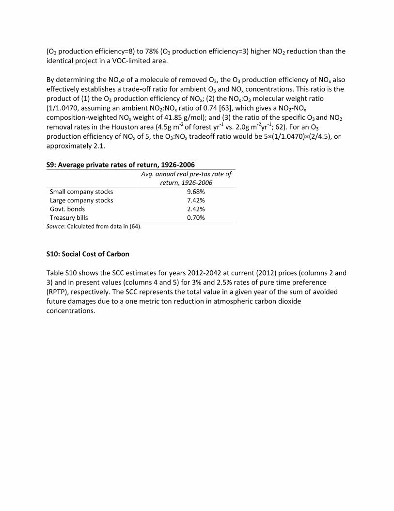
removal rates in the Houston area (4.5g m-2 of forest yr-1 vs. 2.0g m-2yr-1; 62). For an O3 production efficiency of NOx of 5, the O3:NOx tradeoff ratio would be 5×(1/1.0470)×(2/4.5), or approximately 2.1. S9: Average private rates of return, 1926-2006

Type of investment Avg. annual real pre-tax rate of return, 1926-2006

Small company stocks 9.68% Large company stocks 7.42% Govt. bonds 2.42% Treasury bills 0.70%

Source: Calculated from data in (64).

S10: Social Cost of Carbon Table S10 shows the SCC estimates for years 2012-2042 at current (2012) prices (columns 2 and 3) and in present values (columns 4 and 5) for 3% and 2.5% rates of pure time preference (RPTP), respectively. The SCC represents the total value in a given year of the sum of avoided future damages due to a one metric ton reduction in atmospheric carbon dioxide concentrations.

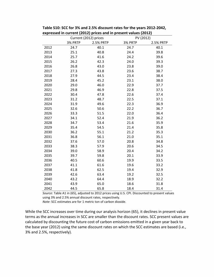
Table S10: SCC for 3% and 2.5% discount rates for the years 2012-2042, expressed in current (2012) prices and in present values (2012) Current (2012) prices PV (2012) 3% PRTP 2.5% PRTP 3% PRTP 2.5% PRTP

2012 24.7 40.1 24.7 40.1 2013 25.1 40.8 24.4 39.8 2014 25.7 41.6 24.2 39.6 2015 26.2 42.3 24.0 39.3 2016 26.8 43.0 23.8 39.0 2017 27.3 43.8 23.6 38.7 2018 27.9 44.5 23.4 38.4 2019 28.4 45.2 23.1 38.0 2020 29.0 46.0 22.9 37.7 2021 29.8 46.9 22.8 37.5 2022 30.4 47.8 22.6 37.4 2023 31.2 48.7 22.5 37.1 2024 31.9 49.6 22.3 36.9 2025 32.6 50.6 22.2 36.7 2026 33.3 51.5 22.0 36.4 2027 34.1 52.4 21.9 36.2 2028 34.7 53.4 21.6 35.9 2029 35.4 54.5 21.4 35.8 2030 36.2 55.1 21.2 35.3 2031 36.8 56.1 21.0 35.1 2032 37.6 57.0 20.8 34.8 2033 38.3 57.9 20.6 34.5 2034 39.0 58.9 20.4 34.2 2035 39.7 59.8 20.1 33.9 2036 40.5 60.6 19.9 33.5 2037 41.1 61.6 19.6 33.2 2038 41.8 62.5 19.4 32.9 2039 42.6 63.4 19.2 32.5 2040 43.2 64.4 18.9 32.2 2041 43.9 65.0 18.6 31.8 2042 44.5 65.8 18.4 31.4

Source: Table A1 in (65), adjusted to 2012 prices using U.S. CPI. Discounted to present values using 3% and 2.5% annual discount rates, respectively. Note: SCC estimates are for 1 metric ton of carbon dioxide.

While the SCC increases over time during our analysis horizon (65), it declines in present value terms as the annual increases in SCC are smaller than the discount rates. SCC present values are calculated by discounting the future cost of carbon emissions emitted in a given year back to the base year (2012) using the same discount rates on which the SCC estimates are based (i.e., 3% and 2.5%, respectively).

References cited in SI 1. Texas Forest Service (2011) Forest management sheet: Cost estimate sheet for forestry

practices. Available at http://txforestservice.tamu.edu/uploadedFiles/Landowners/ Fact%20Sheet%20-%202011%20Forestry%20Practices%20Cost%20Estimate%20Sheet.pdf.

2. Bond J (2006) The Inclusion of Large-Scale Tree Planting in a State Implementation Plan: A Feasibility Study (Davey Resource Group, Geneva, NY).

3. Allen JA, Keeland BD, Stanturf JA, Clewell AF, Kennedy HE, Jr (2001) A guide to bottomland hardwood restoration. General Technical Report SRS-40 (USDA Forest Service Southern Research Station, Ashville).

4. Stanturf JA, Schoenholtz SH, Schweitzer CJ, Shepard JP (2001) Achieving restoration success: myths in bottomland hardwood forests. Restoration Ecology 9(2):189–200.

5. Rosen DJ, De Steven D, Lange ML (2008) Conservation strategies and vegetation characterization in the Columbia Bottomlands, an under-recognized southern floodplain forest formation. Natural Areas Journal 28:74–82.

6. Prasad AM, Iverson LR, Matthews S, Peters M (2007-ongoing) A Climate Change Atlas for 134 Forest Tree Species of the Eastern United States (United States Forest Service, Northern Research Station, Delaware). Available at http://www.nrs.fs.fed.us/atlas/tree/tree_atlas.html#

7. Stanturf JA et al. (2009) Restoration of bottomland hardwood forests across a treatment intensity gradient. For Ecol Manage 257:1803–1814.

8. Lower Mississippi Valley Joint Venture (LMVJV) Forest Resource Conservation Working Group (2007) Restoration, Management, and Monitoring of Forest Resources in the Mississippi Alluvial Valley: Recommendations for Enhancing Wildlife Habitat, eds Wilson R, Ribbeck K, King S, Twedt D (LMVJV, Vicksburg).

9. Wilson R, Twedt D (2005) in Ecology and Management of Bottomland Hardwood Systems: The State of Our Understanding, eds Fredrickson LH, King SL, Kaminski RM (University of Missouri-Columbia), pp 341–352.

10. US Natural Resources Conservation Service (2012) The PLANTS Database (USDA NRCS National Plant Data Team, Greensboro).

11. Staudhammer C et al. (2011) Rapid assessment of change and hurricane impacts to Houston’s urban forest structure. Arboric Urban For 37(2):60–66.

12. Lawrence AB, Escobedo FJ, Staudhammer CL, Zipperer W (2012) Analyzing growth and mortality in a subtropical urban forest ecosystem. Landsc Urban Plan 104(1):85–94.

13. US Natural Resources Conservation Service (2008) Ecological sites: Understanding the landscape (Natural Resources Conservation Service, Washington DC).

14. TCEQ (2004) Revisions to the State Implementation Plan (SIP) for the Control of Ozone Air Pollution, Houston/Galveston/Brazoria (HGB) Ozone Nonattainment Area. Adopted December 1, 2004. Project No. 2004-042-SIP-NR (Texas Commission on Environmental Quality, Austin). Accessed January 25, 2014. http://www.tceq.state.tx.us/implementation/air/sip/sipplans.html#sips

15. TCEQ (2010) Houston-Galveston-Brazoria Attainment Demonstration State Implementation Plan Revision for the 1997 Eight-Hour Ozone Standard. Project No. 2009-017-SIP-NR Adopted March 10, 2010. (Texas Commission on Environmental Quality, Austin). http://www.tceq.state.tx.us/airquality/sip/sipplans.html#sips Accessed January 26, 2014.

16. TCEQ (2013) Houston-Galveston-Brazoria 1997 Eight-Hour Ozone Standard Nonattainment Area Motor Vehicle Emissions Budgets Update State Implementation Plan Revisions. Project Number 2012-002-SIP-NR. (Texas Commission on Environmental Quality, Austin). Adopted April 23, 2013. http://www.tceq.state.tx.us/airquality/sip/sipplans.html#sips (accessed January 26, 2014)

17. World Bank (2012) State and Trends of the Carbon Market 2012 (World Bank, Washington DC).

18. US Environmental Protection Agency (1999) Nitrogen Oxides (NOx), why and how they are controlled. Tech Bull EPA 456/F-99-006R (US Environmental Protection Agency, Research Triangle Park).

19. Krupnick A, McConnell V, Cannon M, Stoessell T, Batz M (2000) Cost-effective NOx control in the eastern United States (Resources For the Future, Washington DC).

20. EME Homer City Generation, L.P. v. EPA, 2012 U.S. App. LEXIS 17535 (D.C. Cir. 2012). 21. US Environmental Protection Agency (2008) Final Ozone NAAQS Regulatory Impact Analysis.

EPA-452/R-08-003 (US Environmental Protection Agency, Research Triangle Park, North Carolina)

22. Federal Register (2010) National Ambient Air Quality Standards for Ozone. Federal Register Proposed Rules 75(11):2938-3052.

23. Federal Register (2013) National Ambient Air Quality Standards for Particulate Matter: Final Rule, Federal Register Rules and Regulations 78(10):3086-3287.

24. 6 NYCRR Subpart 227-2, Reasonable Available Control Technology (RACT) for Major Facilities of Oxides of Nitrogen (NOx). Revised July 8, 2010

25. New York State Department of Environmental Conservation (2013) DAR-20 Economic and Technical Analysis for Reasonably Available Control Technology (RACT). (New York State Department of Environmental Conservation, Albany)

26. San Joaquin Valley Unified Air Pollution Control District (2008) Final Staff Report: Update to Rule 2201 Best Available Control Technology (BACT) Cost Effectiveness Thresholds. (San Joaquin Valley Unified Air Pollution Control District, Modesto).

27. State of California Air Resources Board (2007) ARB Staff Report to the Air Resources Board: Accelerating San Joaquin Valley Air Quality Progress. (State of California Air Resources Board, Sacramento).

28. US Environmental Protection Agency (2004) Incorporating Emerging and Voluntary Measures in a State Implementation Plan (SIP) (US Environmental Protection Agency, Research Triangle Park).

29. Texas Commission on Environmental Quality (2013) Trade Report. March 1, 2013. Available at http://www.tceq.state.tx.us/assets/public/ implementation/air/banking/reports/mect.pdf. Accessed 17 March, 2013.

30. Houston-Galveston Area Council (2006) 2035 Regional Growth Forecast (H-Galveston Area Council, Houston). Available at http://www.h-gac.com/community/socioeconomic/ forecasts/archive/documents/2035_regional_growth_forecast.pdf. Accessed 13March, 2013.

31. Texas Workforce Commission (2010) Gulf Coast WDA Long-term Industry Projections. Available at http://www.tracer2.com/?PAGEID=67&SUBID=114. Accessed 17 March, 2013.

32. Guenther A, Zimmerman PR, Wildermuth M (1994) Natural volatile organic compound emission rate estimates for U.S. woodland landscapes. Atmos Environ 28:1197-1210.

33. Geron C, Harley P, Guenther A (2001) Isoprene emission capacity for US tree species. Atmos Environ 35:3341–3352.

34. Benjamin M, Sudol M, Bloch L, Winer AM (1996). Low-emitting urban forests: A taxonomic methodology for assigning isoprene and monoterpene emission rates. Atmos Environ 30(9):1437–1452.

35. Geron CD, Guenther AB, Pierce TE (1994) An improved model for estimating emissions of volatile organic compounds from forests in the eastern United States. J Geophys Res 99:12773–12791.

36. Kesselmeier J, Staudt M (1999) Biogenic volatile organic compounds (VOC): An overview on emission, physiology and ecology. J Atmos Chem 33:23–88.

37. Karlik JF, McKay AH, Welch JM, Winer AM (2002) A survey of California plant species with a portable VOC analyzer for biogenic emission inventory development. Atmos Environ 36:5221–5233.

38. Karlik JF, Pittenger DR (2012) Urban trees and ozone formation: A consideration for large-scale plantings. Agriculture and Natural Resources Publication 8484 (University of California, Richmond).

39. Nowak DJ et al. (2000) A modeling study of the impact of urban trees on ozone. Atmos Environ 34:1601–1613.

40. Steiner AL et al. (2010) Observed suppression of ozone formation at extremely high temperatures due to chemical and biophysical feedbacks. PNAS 107(46):19685–19690.

41. Sillman S (1999) The relation between ozone, NOx and hydrocarbons in urban and polluted rural environments. Atmos Environ 33(12):1821–1845.

42. Langford AO et al. (2009) Regional and local background ozone in Houston during TexAQS 2006. J Geophys Res 114:D00F12.

43. TexAQS II Rapid Science Synthesis Team (2007) Final Rapid Science Synthesis Report: Findings from the Second Texas Air Quality Study (TexAQS II) (Texas Commission on Environmental Quality, Austin).

44. TCEQ Data Analysis Team (2009) Houston-Galveston-Brazoria Nonattainment Area Ozone Conceptual Model. Draft (Texas Commission on Environmental Quality, Austin). http://www.tceq.texas.gov/assets/public/implementation/air/am/modeling/hgb8h2/doc/ HGB8H2_Conceptual_Model_20090519.pdf (accessed May 12, 2012)

45. Ngan F, Byun D (2011) Classification of weather patterns and associated trajectories of high-ozone episodes in the Houston-Galveston-Brazoria area during the 2005/06 TexAQS-II. J Clim 50(3):485–499.

46. Frost G (2009) Revised TexAQS2K6 HGB Point Source Emission Inventory. Version 1, 7 August, 2009. Downloaded from http://www.esrl.noaa.gov/csd/projects/2006/fieldops/ emission.html. 18May, 2012.

47. Texas Commission on Environmental Quality (No date) IAH Annual (1984-92). Available at http://www.tceq.texas.gov/assets/public/compliance/monops/air/windroses/iahall.gif. Accessed 17 March, 2013.

48. Karl TR, Melillo JM, Peterson TC, eds (2009) Global Climate Change Impacts in the United States (Cambridge University Press, New York).

49. Hogrefe C et al. (2004) Simulating changes in regional air pollution over the eastern United States due to changes in global and regional climate and emissions. J Geophys Res 109: D22301.

50. Tao Z, Williams A, Huang H-C, Caughey M, Liang X-Z (2007) Sensitivity of U.S. surface ozone to future emissions and climate changes. Geophys Res Lett 34:L08811.

51. Tagaris E et al. (2007) Impacts of global climate change and emissions on regional ozone and fine particulate matter concentrations over the United States. J Geophys Res 112:D14312.

52. Nolte CG, Gilliland AB, Hogrefe C, Mickley LJ (2008) Linking global to regional models to assess future climate impacts on surface ozone levels in the United States. J Geophys Res 113: D14307.

53. Jiang X, Wiedinmyer C, Chen F, Yang Z-L, Lo JC-F (2008) Predicted impacts of climate and land use change on surface ozone in the Houston, Texas, area. J Geophys Res 113:D20312.

54. Carter WPL (2010) Development of the SAPRC-07 Chemical Mechanism and Updated Ozone Reactivity Scales (California Air Resources Board, Sacramento).

55. US Environmental Protection Agency (2013) Integrated Science Assessment for Ozone and Related Photochemical Oxidants. EPA 600/R-10/076F. (US Environmental Protection Agency, Research Triangle Park)

56. TCEQ (2014) Air Quality Data and Evaluations: Daily Maximum Eight-Hour Ozone Averages. http://www.tceq.texas.gov/cgi-bin/compliance/monops/8hr_monthly.pl Accessed 7 February 2014.

57. US EPA (2013) 2012 Design Value Report: Ozone. Last updated 7/12/13. Available at http://www.epa.gov/airtrends/values.html Downloaded 2 February 2014.

58. Marshall Research Group (2013) Year-2006 LUR model. http://personal.ce.umn.edu/~marshall/data.php Accessed 5 February 2014.

59. Novotny EV, Bechle MJ, Millet DB, Marshall JD (2012) National satellite-based land-use regression: NO2 in the United States. Environ Sci Technol 45(10):4407–4414.

60. US Environmental Protection Agency (2013) US EPA Green Book: National 8-Hour Ozone (1997) County Map of Maintenance and Nonattainment Areas in the U.S. 5 December 2013. http://www.epa.gov/airquality/greenbk/map8hrnm.html Accessed 5 February 2014

61. US EPA (2013) 2012 Design Value Report: NO2. Last updated 10/22/13. Available at http://www.epa.gov/airtrends/values.html Downloaded 5 February 2014.

62. Nowak DJ, Crane, DE, Stevens JC (2006) Air pollution removal by urban trees and shrubs in the United States. Urban Forestry and Urban Greening 4:115–123.

63. Rivera C et al. (2010) Quantification of NO2 and SO2 emissions from the Houston Ship Channel and Texas City industrial areas during the 2006 Texas Air Quality Study. J Geophys Res 115:D08301.

64. Morningstar (2007) Stocks, Bonds, Bills, and Inflation Data License (Morningstar, Chicago). 65. Interagency Working Group on Social Cost of Carbon (IWGSCC) (2010) Technical Support

Document: Social Cost of Carbon for Regulatory Impact Analysis Under Executive Order 12866 (United States Government, Washington DC).