Shock-Induced Damage in Rocks:Application to Impact Cratering

Thesis by

Huirong Ai

In Partial Fulfillment of the Requirements

for the Degree of

Doctor of Philosophy

California Institute of Technology

Pasadena, California

2006

(Defended May 8, 2006)

ii

c© 2006

Huirong Ai

All Rights Reserved

iii

To My Parents

iv

Acknowledgements

I would like to express my sincere gratitude to my thesis advisor, Thomas Ahrens, who

gave me the chance to explore the shockwave field, and supported me both spiritually and

financially, in a very generous way, through the past years. His enthusiasm toward science,

and amazing supervision over the group have always impressed me and will benefit my

career in the future.

I need extend my greatest gratitude to my thesis committee, Jason Saleeby, who is

also my academic advisor, Rob Clayton, and Guruswami Ravichandran for their trust, un-

derstanding, support, encouragement, and valuable feedback despite their busy schedules.

Also thanks to Ken Farley for his support. Special thanks to Ravi for letting me use the

ultrasonic apparatus in his lab.

This thesis would not have been possible without the support of the whole shockwave

group. I express my appreciation to Mike Long, Papo Gelle, and Russell Oliver for their

assistance with my experiments, as well as to Sue Yamada, for her excellent cooking, the

inspiration on knitting and crocheting during free time, and her kindness to us international

students. I benefited a lot from discussions with Andy Shen, Michael Willis, Mikhail Ra-

shev, Daoyuan Sun, Shenlian Luo, and Michael Heinrich. Also, the time spent at work

became more enjoyable because of them.

v

I am very grateful to Joann Stock, Rob Clayton, and Mark Simons for the help during

my oral projects. Especially to Joann and Rob for the support during my first three years,

and their patience with the Manihiki paper, although I did not include it in this thesis.

I owe a lot to all the previous and present members of Seismological lab, in particular,

Sidao Ni, Chen Ji, Kaiwen Xia, Magali Billen, Patricia Persaud, Leo Eisner, and Sarah

Stewart, who were always patient to answer all kinds of questions I had. In the meantime,

my journey at Caltech became so meaningful and enjoyable because of my officemates and

my friends. Thank you for your company and sharing the great moments in my life.

Finally but foremost, I would like to express my deepest gratitude to my parents for

their endless love, unconditional support, and the sacrifice they made for me all these years.

Without them, it is impossible for me to reach this point of my life. And this dissertation is

dedicated to them.

vi

Abstract

Shock-induced damage beneath impact craters is studied in this work. Two representative

terrestrial rocks, San Marcos granite and Bedford limestone, are chosen as test target. Im-

pacts into the rock targets with different combinations of projectile material, size, impact

angle, and impact velocity are carried out at cm scale in the laboratory.

Shock-induced damage and fracturing would cause large-scale compressional wave ve-

locity reduction in the recovered target beneath the impact crater. The shock-induced dam-

age is measured by mapping the compressional wave velocity reduction in the recovered

target. A cm scale nondestructive tomography technique is developed for this purpose. This

technique is proved to be effective in mapping the damage in San Marcos granite, and the

inverted velocity profile is in very good agreement with the result from dicing method and

cut open directly. But it is not a good method for Bedford limestone, since the wave atten-

uation is too high to have a recordable signal. Instead, dicing method is used for studying

the shock-induced damage in Bedford limestone.

Both compressional velocity and attenuation are measured in three orthogonal direc-

tions on cubes prepared from one granite target impacted by a lead bullet at 1200 m/s.

Anisotropy is observed from both results, but the attenuation seems to be a more useful

parameter than acoustic velocity in studying orientation of cracks.

vii

Our experiments indicate that the shock-induced damage is a function of impact condi-

tions including projectile type and size, impact velocity, and target properties. Combined

with other crater phenomena such as crater diameter, depth, ejecta, etc., shock-induced

damage would be used as an important yet not well recognized constraint for impact his-

tory.

The shock-induced damage is also calculated numerically to be compared with the

experiments for a few representative shots. The Johnson-Holmquist strength and failure

model, initially developed for ceramics, is applied to geological materials. Strength is a

complicated function of pressure, strain, strain rate, and damage. The JH model, coupled

with a crack softening model, is used to describe both the inelastic response of rocks in

the compressive field near the impact source and the tensile failure in the far field. The

model parameters are determined either from direct static measurements, or from indirect

numerical adjustment. The agreement between the simulation and experiment is very en-

couraging.

viii

Contents

Acknowledgements iv

Abstract vi

1 Introduction and Background 1

1.1 Background . . . . . . . . . . . . . . . . . . . . . . . . . . . . . . . . . .1

1.2 Organization of this dissertation . . . . . . . . . . . . . . . . . . . . . . .4

2 Dynamic Tensile Strength of Terrestrial Rocks 5

2.1 Introduction . . . . . . . . . . . . . . . . . . . . . . . . . . . . . . . . . .5

2.2 Significance and lithologies of rocks . . . . . . . . . . . . . . . . . . . . .6

2.3 Experimental techniques . . . . . . . . . . . . . . . . . . . . . . . . . . .8

2.4 Results and discussion . . . . . . . . . . . . . . . . . . . . . . . . . . . .13

2.4.1 Reduction of velocity by cracks . . . . . . . . . . . . . . . . . . .26

2.4.2 Interpretation of Vp/Vs . . . . . . . . . . . . . . . . . . . . . . . . 29

2.4.3 Strain-rate effect . . . . . . . . . . . . . . . . . . . . . . . . . . .30

2.5 Conclusion . . . . . . . . . . . . . . . . . . . . . . . . . . . . . . . . . .32

3 Tomography Study of Shock-Induced Damage beneath Craters 34

ix

3.1 Introduction . . . . . . . . . . . . . . . . . . . . . . . . . . . . . . . . . .34

3.2 Experimental procedure . . . . . . . . . . . . . . . . . . . . . . . . . . . .35

3.2.1 Cratering . . . . . . . . . . . . . . . . . . . . . . . . . . . . . . .35

3.2.2 Tomography technique . . . . . . . . . . . . . . . . . . . . . . . .35

3.3 Results and discussion . . . . . . . . . . . . . . . . . . . . . . . . . . . .41

3.3.1 Tomography inversion . . . . . . . . . . . . . . . . . . . . . . . .41

3.3.2 Test problems . . . . . . . . . . . . . . . . . . . . . . . . . . . . .43

3.3.3 Experimental results . . . . . . . . . . . . . . . . . . . . . . . . .47

3.4 Concluding remarks . . . . . . . . . . . . . . . . . . . . . . . . . . . . . .61

4 Effects of Shock-Induced Cracks on the Ultrasonic Velocity and Attenuation

in Granite 62

4.1 Introduction . . . . . . . . . . . . . . . . . . . . . . . . . . . . . . . . . .62

4.2 Experimental technique . . . . . . . . . . . . . . . . . . . . . . . . . . . .64

4.3 Experimental results . . . . . . . . . . . . . . . . . . . . . . . . . . . . .69

4.3.1 Compressional wave velocity measurements . . . . . . . . . . . . .69

4.3.2 Attenuation measurements . . . . . . . . . . . . . . . . . . . . . .74

4.4 Analysis and discussion . . . . . . . . . . . . . . . . . . . . . . . . . . . .76

4.5 Concluding remarks . . . . . . . . . . . . . . . . . . . . . . . . . . . . . .84

5 Scaling Law 86

5.1 Introduction . . . . . . . . . . . . . . . . . . . . . . . . . . . . . . . . . .86

5.2 Dimensional analysis . . . . . . . . . . . . . . . . . . . . . . . . . . . . .87

5.3 Experimental data and discussion . . . . . . . . . . . . . . . . . . . . . . .90

x

5.4 Summary . . . . . . . . . . . . . . . . . . . . . . . . . . . . . . . . . . .102

6 Shock-Induced Damage beneath Oblique Impact Craters 104

6.1 Introduction . . . . . . . . . . . . . . . . . . . . . . . . . . . . . . . . . .104

6.2 Experiments . . . . . . . . . . . . . . . . . . . . . . . . . . . . . . . . . .107

6.3 Results and discussion . . . . . . . . . . . . . . . . . . . . . . . . . . . .107

6.3.1 Experimental results . . . . . . . . . . . . . . . . . . . . . . . . .107

6.3.2 Discussion . . . . . . . . . . . . . . . . . . . . . . . . . . . . . .115

6.4 Conclusion . . . . . . . . . . . . . . . . . . . . . . . . . . . . . . . . . .119

7 Numerical Modelling of Shock-Induced Damage for Granite under Dynamic

Loading 121

7.1 Introduction . . . . . . . . . . . . . . . . . . . . . . . . . . . . . . . . . .121

7.2 Related work . . . . . . . . . . . . . . . . . . . . . . . . . . . . . . . . .123

7.2.1 An overview of AUTODYN . . . . . . . . . . . . . . . . . . . . .123

7.2.2 Description of brittle material model . . . . . . . . . . . . . . . . .124

7.2.2.1 JH-2 model . . . . . . . . . . . . . . . . . . . . . . . .124

7.2.2.2 Tensile crack softening model . . . . . . . . . . . . . . .127

7.3 Determination of model constants for granite . . . . . . . . . . . . . . . .128

7.3.1 Pressure . . . . . . . . . . . . . . . . . . . . . . . . . . . . . . . .128

7.3.2 Strength . . . . . . . . . . . . . . . . . . . . . . . . . . . . . . . .131

7.3.3 Damage . . . . . . . . . . . . . . . . . . . . . . . . . . . . . . . .133

7.3.4 Tensile cracking softening . . . . . . . . . . . . . . . . . . . . . .134

7.4 Examples . . . . . . . . . . . . . . . . . . . . . . . . . . . . . . . . . . .134

xi

7.4.1 Lead bullet impacting granite . . . . . . . . . . . . . . . . . . . .134

7.4.2 Copper ball impacting granite . . . . . . . . . . . . . . . . . . . .140

7.4.3 Plate impact of Al flyer plate into granite . . . . . . . . . . . . . .140

7.4.4 Oblique impact . . . . . . . . . . . . . . . . . . . . . . . . . . . .141

7.4.5 Effect of gravity on damage and cracks . . . . . . . . . . . . . . .146

7.5 Conclusion . . . . . . . . . . . . . . . . . . . . . . . . . . . . . . . . . .146

8 Future Work 148

xii

List of Figures

1.1 Schematic illustration of pressure near site of an impact by a projectile at 10

km/s and its implication for final state of target. . . . . . . . . . . . . . . . .3

2.1 One-dimensional impact setup showing recovery tank, sample, and alignment.10

2.2 Recovered samples showing radial and spall cracks. . . . . . . . . . . . . . .14

2.3 Velocity measurements for San Marcos gabbro experiments. . . . . . . . . .21

2.4 Velocity measurements for San Marcos granite experiments. . . . . . . . . .22

2.5 Velocity measurements for Sesia eclogite experiments. . . . . . . . . . . . .23

2.6 Velocity measurements for Coconino sandstone experiments of duration time

of (a) 2.4µs and (b) 1.4µs. Dashed lines indicate the same as those in Figure

2.5. . . . . . . . . . . . . . . . . . . . . . . . . . . . . . . . . . . . . . . .24

2.7 Velocity measurements for Bedford limestone. (a) 0.5µs and (b) 1.3µs.

(FromAhrens and Rubin[1993], Fig. 2.) . . . . . . . . . . . . . . . . . . .25

2.8 Post-shotVp/Vs values versus computed tensile stress. . . . . . . . . . . . .27

2.9 Normalized tensile strengths as a function of strain rate for ice and rocks. . .32

3.1 (a) Cross section of tomography measurement setup; (b) Enlarged side view

of position of 0.08 cm diameter steel impactor sphere. . . . . . . . . . . . .36

3.2 Typical ultrasonic source and receiver signal. . . . . . . . . . . . . . . . . .37

xiii

3.3 Tomographic straight ray diagram for pre-shot San Marcos granite. . . . . .39

3.4 Tomographic straight ray diagram for post-shot San Marcos granite. . . . . .40

3.5 Test of the cm-scale tomography method developed above using a homoge-

nous velocity structure. (a) Forward velocity model. Velocity of the 20x15

cm structure is 6.4 km/s; (b) Inverted velocity structure using the tomogra-

phy method with straight ray assumption. . . . . . . . . . . . . . . . . . . .45

3.6 Test of the cm-scale tomography method developed above using a heteroge-

nous velocity structure. (a) Forward velocity structure; (b) Inverted velocity

structure. . . . . . . . . . . . . . . . . . . . . . . . . . . . . . . . . . . . .46

3.7 Inversion solution of compressional wave velocity structure of pre-shot San

Marcos granite using straight ray deploy. . . . . . . . . . . . . . . . . . . .48

3.8 Compressional wave velocity structure of post-shot San Marcos granite of

shot 117 from top surface to depth of 10 cm using straight ray deploy. . . . .49

3.9 Diagram showing minimum travel time rule for a stress wave traveling be-

tween point A and point B. . . . . . . . . . . . . . . . . . . . . . . . . . . .50

3.10 . . . . . . . . . . . . . . . . . . . . . . . . . . . . . . . . . . . . . . . . .51

3.10 Diagram of procedure to obtain minimum time path from source (S) to re-

ceiver (R). . . . . . . . . . . . . . . . . . . . . . . . . . . . . . . . . . . . .52

3.11 Diagram showing a few typical curve ray paths using method described in

Figure 3.10 and shown velocity model. . . . . . . . . . . . . . . . . . . . .53

3.12 Comparison of straight ray and curve ray assumption for the second iteration.54

xiv

3.13 Histogram of relative error to measured value. (a) For straight ray assump-

tion; (b) For curve ray assumption, second iteration. . . . . . . . . . . . . . .55

3.14 Histogram of relative error to measured value for curve ray assumption,

fourth iteration. . . . . . . . . . . . . . . . . . . . . . . . . . . . . . . . . .56

3.15 Diagonal values of model resolution matrix. (a) Matrix plot of the4th iter-

ation; (b) Comparison for four iterations, cells 1 to 200 (See Figure 3.3 for

cell index). . . . . . . . . . . . . . . . . . . . . . . . . . . . . . . . . . . .57

3.16 Compressional wave velocity structure of post-shot San Marcos granite of

shot 117 from top surface to depth of 10 cm. . . . . . . . . . . . . . . . . .58

3.17 Cross section of shot 117, recovered granite impacted by 3.2 g lead bullet

at 1200 m/s showing different types of cracks and damage depth. Cracks

highlighted by dye coolant. . . . . . . . . . . . . . . . . . . . . . . . . . . .59

4.1 Pulse transmission ultrasonic system (modified fromWeidner[1987]). . . . . 64

4.2 Sketch of attenuation measurement system (modified fromWinkler and Plona

[1982]). . . . . . . . . . . . . . . . . . . . . . . . . . . . . . . . . . . . . .65

4.3 Typical ultrasonic record for attenuation measurements and spectral ampli-

tude of signals. . . . . . . . . . . . . . . . . . . . . . . . . . . . . . . . . .67

4.4 Calculated relative spectral amplitude of signals. Peak amplitude for surface

A happens at frequency∼ 4.5 MHz. . . . . . . . . . . . . . . . . . . . . . .68

4.5 P wave velocities as a function of distance from z axis at indicated depths

within sample. (a) x direction; (b) y direction; (c) z direction. . . . . . . . . .71

xv

4.6 P wave velocities as a function of distance from z axis in x, y and z directions

at 4.5 cm depth below surface. . . . . . . . . . . . . . . . . . . . . . . . . .72

4.7 Plot of all velocity measurements in three directions as function of distance

from crater center. . . . . . . . . . . . . . . . . . . . . . . . . . . . . . . .73

4.8 Attenuation coefficients as a function of normalized radial distance from im-

pact point for three directions. Lines are power decay fit of data. (a) x; (b) y;

(c) z. . . . . . . . . . . . . . . . . . . . . . . . . . . . . . . . . . . . . . .75

4.9 Schematic diagram showing effect of aligned cracks on elastic waves propa-

gating at different directions. . . . . . . . . . . . . . . . . . . . . . . . . . .77

4.10 Damage parameters as a function of normalized radial distance from impact

point for three directions. Lines are power decay fit of data. . . . . . . . . .79

4.11 Crack densities inverted from measured P-wave velocity by using model of

O’Connell and Budiansky[1974] as function of normalized radial distance

from impact point for three directions. Lines are power decay fit of data. (a)

x; (b) y; (c) z. . . . . . . . . . . . . . . . . . . . . . . . . . . . . . . . . . .81

4.12 Attenuation coefficients versus damage parameter for three directions. (a) x;

(b) y; (c) z. Lines are linear fit of data. . . . . . . . . . . . . . . . . . . . . .82

5.1 Shot 1208, granite impacted by∼25 g lead ball (with sabot) at 800 m/s.

Scale is 5 cm. . . . . . . . . . . . . . . . . . . . . . . . . . . . . . . . . . .96

5.2 Shot 1209, limestone impacted by∼16 g (with sabot) lead ball at 590 m/s.

Scale is 5 cm. . . . . . . . . . . . . . . . . . . . . . . . . . . . . . . . . . .97

xvi

5.3 Normalized crater damage depth by apparent projectile radius,Dd/apa, over

projectile-density ratio,ρp/ρt, as power-law function of strength parameter,

π3 = Y/ρtU2. . . . . . . . . . . . . . . . . . . . . . . . . . . . . . . . . . .99

5.4 Normalized crater volume by apparent projectile volume,ρtV/m as a func-

tion of strength parameter,π3. . . . . . . . . . . . . . . . . . . . . . . . . .100

5.5 Plot of crater depth as a function of crater diameter. Linear relation is ob-

served, and slope is 0.12. . . . . . . . . . . . . . . . . . . . . . . . . . . . .101

6.1 Peak shock pressure contours in the plane of impact for a series of 3D hy-

drocode simulations at various impact angles. . . . . . . . . . . . . . . . . .106

6.2 (a) Oblique impact geometry. Tomography measurement carried out on two

central planes; (b) Diagram showing orientation for dicing method for lime-

stone. . . . . . . . . . . . . . . . . . . . . . . . . . . . . . . . . . . . . . .108

6.3 Inverted compressional wave profiles of two planes for oblique impact crater

in San Marcos granite, shot No. 121, using tomography method. . . . . . . .110

6.4 Inverted compressional wave profiles of same central planes as in Figure 6.3,

except that 1 cm top surface layer is cut off. See Figure 6.3 for explanation

of Vectors. (a) Plane A; (b) Plane B. . . . . . . . . . . . . . . . . . . . . . .111

6.5 Compressional wave profiles of two planes for oblique impact crater in Bed-

ford limestone, shot 122, using dicing method. . . . . . . . . . . . . . . . .115

6.6 Compressional wave profiles of plane B for shot 122 using dicing method.

All notes same as in Figure 6.5. (a) x direction; (b) z direction. Asymmetry

is not observed. . . . . . . . . . . . . . . . . . . . . . . . . . . . . . . . . .116

xvii

7.1 Description of JH2 model for brittle materials (fromJohnson and Holmquist

[1999], Figure 1). . . . . . . . . . . . . . . . . . . . . . . . . . . . . . . . .125

7.2 Strength, damage, and fracture under a constant pressure and strain rate for

the JH2 model (fromJohnson and Holmquist[1999], Figure 2). . . . . . . .127

7.3 Test data and model for shock pressure-volume response of granite. . . . . .130

7.4 Test data and model for strength of intact and damaged granite. . . . . . . . .131

7.5 (a) Initial setup for simulating shot 117, lead bullet into 20x20x15 cm granite

block at velocity of 1.2 km/s, and location of gauge points; (b) Peak pressure

of gauges versus normalized distance from impact.r is distance,a is radius

of projectile. Red line is exponential fit of data. . . . . . . . . . . . . . . . .136

7.6 Simulated damage contour for shot 117 at several times during impact event.137

7.7 Cross section of granite impacted by lead bullet at 1200 m/s illustrating crack

distribution. Normal impact. (a) Experimental result; (b) AUTODYN-2D

simulation at 0.03 ms. Left panel illustrates material status; right panel illus-

trates damage. . . . . . . . . . . . . . . . . . . . . . . . . . . . . . . . . . .138

7.8 Cross section of granite impacted by copper ball at 690 m/s. Normal impact.

(a) experimental result; (b) simulation at 0.04 ms. Others are the same as in

Figure 7.7b. . . . . . . . . . . . . . . . . . . . . . . . . . . . . . . . . . . .139

7.9 Simulated damage for plate impact of Aluminum flyer plate into San Marcos

granite at different velocities. Flyer plate not shown here. . . . . . . . . . . .142

7.10 Cross section of granite impacted by copper ball at 1000 m/s, experimental

result.Vectorshows impact angle at 450. Visible tensile cracks are highlighted.143

xviii

7.11 Simulated result at 0.1 ms for shot shown in Figure 7.10. . . . . . . . . . . .144

7.12 Simulated result shown effect of gravity on formation of tensile cracks. Nor-

mal impact. (a) 500g, ap=3 mm; (b) 1g, ap=1500 mm. Left panel illustrates

material status, right panel for damage status. Notice different scales on the

two plots. See text for discussion. . . . . . . . . . . . . . . . . . . . . . . .145

xix

List of Tables

2.1 Mineralogical composition of San Marcos granite . . . . . . . . . . . . . . .7

2.2 Physical properties of experimental materials . . . . . . . . . . . . . . . . .9

2.3 One-dimensional tensile strain impact parameters and pre-shot and post-shot

ultrasonic compressional and shear velocities. . . . . . . . . . . . . . . . . .15

2.4 Tensile strengths (in MPa) of ice and rocks at different strain rates. . . . . . .31

4.1 Compressional wave velocity beneath impact crater in San Marcos granite,

shot 117. . . . . . . . . . . . . . . . . . . . . . . . . . . . . . . . . . . . .70

5.1 Summary of experimental parameters . . . . . . . . . . . . . . . . . . . . .91

6.1 Compressional wave velocity beneath oblique impact crater in Bedford lime-

stone, shot 122, plane A, along projectile trajectory. . . . . . . . . . . . . . .113

6.2 Compressional wave velocity beneath oblique impact crater in Bedford lime-

stone, shot 122, plane B, Normal to projectile trajectory. . . . . . . . . . . .114

7.1 JH2 baseline and crack softening constants for granite . . . . . . . . . . . .129

7.2 One-dimensional impact parameters, as well as pre- and post-shot compres-

sional wave velocities for Al2024 flyer plate into San Marcos granite. . . . .133

1

Chapter 1

Introduction and Background

1.1 Background

Impact cratering is a universal process in the solar system. Significant geophysical features

for impact craters include gravity and magnetic anomaly, electrical property change of

rocks such as resistivity below impact craters, seismic profiles showing low velocity zone,

etc [Pilkington and Grieve, 1992]. These features are caused directly or indirectly by the

precedence of shock-induced damage and cracks in rocks beneath the crater, which in turn

are related to the pressure profiles in the impacted targets.

The peak shock pressure in an impacted target displays four regimes [Ahrens and

O’Keefe, 1987]. Regime 1 is the impedance match regime, extending to a few projec-

tile radii into the target, where the peak shock pressure is roughly given by the planar

impedance match method [Ahrens, 1987]. Since materials achieve peak shock pressure,

rock is vaporized upon impacts of>10 km/s, melted upon impact of>5 km/s and is mas-

sively powdered at>1 km/s. Regime 2 is the shock decay regime, which extends to the

distance where the pressure equals the Hugoniot elastic limit (HEL) of the target. Pressure

in this regime at distancer from the impact point, Pr, follows the relation [Ahrens and

2

O’Keefe, 1987]:

Pr = P0 (r/r0)−n (1.1)

wherer0 is the radius of the projectile andn is the attenuation index. For nonporous silicate

projectile and target,n is defined as:

n u −0.625log10U − 1.25 (1.2)

whereU is the impact velocity. Shear and concentric cracks are formed in this regime.

Beyond this is regime 3, the elastic decay regime. The magnitude of tensile stress in this

regime is in the same order of the shear stress [Shibuya and Nakahara, 1968], and radial

tensile cracks are produced when the tensile tangential stress exceeds the dynamic tensile

strength of the material. Regime 4 is the spalling region near the surface.Melosh[1989]

has a similar definition for an impact at 10 km/s into the rock target: I. melting; II. region

where pressure exceeds HEL; III. Grady-Kipp fragments region, which is defined to be

resulted from dynamic tensile stress; IV. spalling region (Figure 1.1).

Damage and cracking in a fractured body reduce the effective elastic moduli of the

media, which in turn reduce the elastic velocities [e.g.O’Connell and Budiansky, 1974;

Kachanov, 1993]. Large scale reduction in compressional wave velocity from the intrinsic

value caused by the shock-induced cracking of rocks beneath impact craters has long been

recognized both in the field [Ackermann et al., 1975;Pohl et al., 1977], and in small-scale

craters in the laboratory [Ahrens and Rubin, 1993;Xia and Ahrens, 2001]. For the Moon,

the whole crust suffers shock-induced damage according toSimmons et al.[1973].

3

Figure 1.1: Schematic illustration of pressure near the site of an impact and its implicationfor final state of target. Tensile stresses break rock into Grady-Kipp fragments to greatdepths below impact site. (FromMelosh[1989], Figure 5.4, p. 64).

Xia and Ahrens[2001] performed preliminary impact cratering recovery experiments

and mapped the damage zones using ultrasonic measurements based on the fact that the

shock-induced damage beneath the impact craters would cause large scale compressional

wave velocity deficit in the target rocks. They suggested that shock-induced damage and

cracking beneath craters, if combined with other constraints such as crater dimension, phys-

ical properties of target and projectile obtained from field mapping, could provide important

information about the impact conditions.

However, the shock-induced damage beneath impact craters as a potential constraint has

not been systematically studied yet. In this work, study of shock-induced damage beneath

craters is carried out at cm scale in the laboratory. Two types of rocks, San Marcos granite

and Bedford limestone, are chosen in this work for damage study, since they are represen-

tative of crustal rocks. In parallel, numerical simulation is performed and compared with

4

experimental results.

1.2 Organization of this dissertation

From the discussion above, the dynamic fracture behavior of rocks plays an important role

in the impact process. For this reason, determination of dynamic tensile strength for four

representative terrestrial rocks is first discussed in chapter 2. Chapter 3 describes the newly

developed cm scale nondestructive tomography method for mapping the low velocity zone

caused by the shock-induced damage and fracturing. The inverted compressional wave

velocity profile of one shot, lead bullet launched into a granite target at 1200 m/s, is also

shown and compared with the experimental result. After tomography mapping, the same

recovered granite target is cut open, and 1 cm cubes are prepared from the center plane for

ultrasonic velocity and attenuation measurement. Both results from dicing are presented

and discussed in chapter 4. Chapter 5 presents the damage data for the shots carried on in

this work for both granite and limestone. A simple scaling law is obtained from the exper-

iments. All the shots in chapter 5 are performed at a vertical angle to the impact surface.

However, natural impact craters always happen at impact angles less than vertical [Gilbert,

1893;Shoemaker, 1962]. Therefore, a few oblique impacts are carried out to study the

effect of impact angles on shock-induced damage. Damage information for these oblique

impacts is presented in Chapter 6. The last chapter explores the numerical simulation of

damage below impact craters. Johnson-Holmquist [Johnson and Holmquist, 1999] strength

model is applied to geological materials for the first time. Several calculations are done and

compared with available experimental data.

5

Chapter 2

Dynamic Tensile Strength of TerrestrialRocks

2.1 Introduction

The dynamic fracture behavior of rocks plays an important role in fracturing and fragmen-

tation procedures, which vary from industrial processes, such as coal and oil shale frag-

mentation [Murri et al., 1977], quarrying and mining operations [Carter, 1978], impact or

explosive crater formation [O’Keefe and Ahrens, 1976], and accretion of planetesimals in

the early stages of planetary formation [Matsui and Mizutani, 1977].

Dynamic tensile strength experiments on rocks have been carried out byGrady and

Hollenbach[1979],Cohn and Ahrens[1981],Lange et al.[1984],Ahrens and Rubin[1993]

and others. Previously, three quantitative methods have been used to determine the dy-

namic tensile strength. These are: (1) the free-surface velocity pullback signal method

[Grady and Hollenbach, 1979]; (2) terminal examination [Cohn and Ahrens, 1981;Lange

et al., 1984]; and (3) ultrasonic post-impact examination [Ahrens and Rubin, 1993]. The

free-surface velocity pullback signal method measures the drop in the target’s free-surface

velocity upon arrival of the compression wave generated by an expanding tensile crack to

6

determine tensile strength. Method 2 involves microscopic examination of polished thin

section made from the recovered samples to determine the incipient spall cracks produced

by impact. The stress above which microscopically observable cracks appear is assumed

to be the dynamic tensile strength. Post-impact ultrasonic examination measures the pre-

and post-shot ultrasonic velocities of the samples and relates the shock-induced damage in

rocks to shock-induced one-dimensional tensile stresses. The tensile strengths determined

by the free-surface velocity pullback signal method and the terminal examination depends

crucially on the properties along the narrow zone of tensile failure where the rock fractures.

Moreover we note that the sample-cutting process required to examine recovered samples

in method 2 could produce additional damage. The ultrasonic method is a superior method

and it is a volume measurement. This method measures crack density instead of the prop-

erties of a single crack. For this reason, ultrasonic method 3 is chosen to determine the

tensile strength in this work.

Quantitative data on the tensile behavior of many types of rocks and its dependence on

strain rate are still lacking. In this study we selected two igneous rocks (San Marcos gabbro

and granite), one sedimentary rock (Coconino sandstone) and one metamorphic rock (Sesia

eclogite) for determination of the dynamic tensile strength using method 3 above.

2.2 Significance and lithologies of rocks

San Marcos gabbro from Escondido, a well-studied rock [Lange et al., 1984;Ahrens and

Rubin, 1993;Xia and Ahrens, 2001], is chosen for comparison with previous studies.Lange

et al. [1984] reported that the density of this rock is 2.867 g/cm3, the dynamic tensile

7

strength is 150 MPa, the compressional wave velocity (Vp) is 6.36± 0.16 km/s, and it has

very low initial crack density. The mineral composition of San Marcos gabbro is 67.9% pla-

gioclase, 22.5% amphibole, 2.6% pyroxene, 1.4% quartz and some trace elements [Lange

et al., 1984].

San Marcos granite is also chosen because this is the rock target used for this project.

This intrusive granite has the same originality (Escondido, California) as San Marcos gab-

bro. Mineralogical composition obtained by Scanning Electron Microscopy (SEM) of the

thin section for San Marcos granite is shown in Table 2.1. The grain size of quartz and pla-

gioclase is 1 to 2 mm, intergrown with dark minerals including amphibole and some biotite

grains, size of which is 1 to 2 mm. On a microscopic level, the rock is essentially crack-free

except for microcracks along grain boundaries. The density of San Marcos granite is 2.657

g/cm3, the intrinsic compressional wave velocity (Cp) is 6.31± 0.1 km/s, determined at 1

MHz.

Table 2.1: Mineralogical composition of San Marcos graniteMineral Area (%)Quartz 20.9Plagioclase 51.0Amphibole 25Biotite 0.9Fe2O3 0.9Alkali feldspar traceTotal 98.7

The dynamic tensile strength of Coconino sandstone from Meteor Crater, Arizona is

of interest, as Coconino sandstone is one of the main sedimentary rock types of the crater

[Shoemaker, 1963]. The subsurface strata of Meteor Crater have been studied in a refrac-

tion survey [Ackermann et al., 1975]. Roddy et al.[1980] simulated the formation of this

8

crater. However, previously only dynamic compressive experiments at different strain rates

were performed byAhrens and Gregson[1964] andShipman et al.[1971] on this type of

rock. The block from which the samples are made is yellowish-gray or cream colored, con-

tains sub-parallel laminae that are separated by thin laminae containing more than average

amounts of silt and clay sized grains. Cross-bedding can be seen clearly on the cutting sur-

faces. Coconino sandstone is composed of 97% quartz, 3% feldspar, with traces of clay and

heavy minerals [Ahrens and Gregson, 1964]. Average grain size is in the range of 0.12-0.15

mm and porosity is 24-25% [Ahrens and Gregson, 1964;Shipman et al., 1971]. The bulk

density of our samples was 2.08± 0.03 g/cm3, slightly higher than that reported byAhrens

and Gregson[1964] andShipman et al.[1971] of 1.99 g/cm3. Impact and ultrasonic wave

measurements are all normal to the bedding of the sandstone. Eclogite is chosen because

it may represent the upper limit of dynamic tensile strength available for terrestrial rocks.

The eclogite from Sesia zone of the Austroalpine system in Italy is metamorphic. Thin

section analysis of the rock sample shows that it contains 40% garnet, 45% clinopyroxene,

4% mica, trace feldspar and opaques. Grain size is 1∼ 1.5 mm, and the bulk density is

3.44± 0.04 g/cm3.

The physical properties of the four types of rocks are listed in Table 2.2.

2.3 Experimental techniques

The dynamic tensile strengths of the San Marcos gabbro, Coconino sandstone, and Sesia

eclogite were determined by planar impact experiments using a 40 mm compressed gas

gun, similar to that described in [Cohn and Ahrens, 1981]. A Lexan projectile carrying a

9

Table 2.2: Physical properties of experimental materialsMaterial Averageρ, g/cm3 Cp, km/s Cs, km/sSan Marcos gabbro 2.8672 6.651 3.571

6.362

San Marcos granite 2.661 6.41 3.571

Coconino sandstone 2.081 2.811 1.821

(velocity normal to bedding) 1.993

Sesia ecologite 3.441 6.401 3.781

PMMA 1.2 2.8Aluminum 2024 2.78 6.36

Sources:1This study;2Lange et al.[1984]; 3Ahrens and Gregson[1964].

polymethyl methacrylate (PMMA) or aluminum (Al) flyer plate at its front is accelerated

by the expansion of precompressed air to velocities in the 5 to 60 m/s range (Figure 2.1).

The initial impact produces compressional shock waves propagating forward into the target

and back into the flyer plate. These compressional waves then reflect back as relief waves

from the free surfaces of the target and the flyer plate. Tension is produced when the two

relief waves meet within the sample. We assume that the magnitude of the tensile stress is

equal to that of the original compressive stress, and the initial compressive pulse produced

no detectable damage. When the peak tensile stress exceeds the dynamic tensile strength

of the rock, cracks start to occur within the sample.

10

40m

mG

un M

uzzl

e

Com

pres

sed

Air

Tim

ing

Las

ers

(for

pro

ject

ileV

eloc

ityM

easu

rem

ent )

Alig

nmen

tPl

ate

Air

Lex

anPr

ojec

tile

Al o

rPM

MA

Flye

rPl

ate

Rec

over

y Ta

nk

Abs

orba

ntR

ages

Roc

k Ta

rget

Fig

ure

2.1:

Ske

tch

ofon

e-di

men

sion

alim

pact

setu

psh

owin

gre

cove

ryta

nk,

sam

ple,

and

alig

nmen

t.D

iscs

ofro

ck22

∼23

mm

indi

amet

eran

d6.

5∼7

mm

inth

ickn

ess

wer

ein

sert

edin

toa

stee

lal

ignm

ent

plat

e.Le

xan

proj

ectil

esfit

ted

with

Alu

min

um(A

l)or

poly

met

hylm

etha

cryl

ate

(PM

MA

)fly

erpl

ates

impa

cted

the

sam

ple.

Velo

city

ofpr

ojec

tile

isde

term

ined

byla

ser

beam

s.F

ollo

win

gim

pact

rock

targ

etfli

esin

toa

clot

hre

cove

ryta

nk,w

here

itis

prot

ecte

dfr

omfu

rthe

rda

mag

e.

11

The choice of PMMA or Al flyer plates depends on the impedances of the rock, defined

as the product of the density,ρ, and the compressional velocity,Vp. Al flyer plates are used

for San Marcos Gabbro and Sesia Eclogite, with impact velocities of 13 to 30 m/s, and 24

to 60 m/s respectively. PMMA flyer plates are used for Coconino sandstone, with impact

velocities of 5 to 22 m/s. The impact velocities are controlled by varying the pressure of

the compressed air. Different impact velocities result in different amplitude tensile stresses.

The impact velocity is measured in air by the sequential interruption of three laser beams.

The impacted target flies free into a recovery tank, where loose rags prevent further damage.

The targets are shaped as discs with diameters of 22 to 23 mm and thickness of 6.5 to 7

mm. Front and rear surfaces are polished. The achieved parallelism of the sample surfaces

was±0.003 mm for San Marcos gabbro and Sesia eclogite. Surface parallelism ensures that

the strain in the∼ 1 cm central region of the sample is approximated by a one-dimensional

strain condition. Less parallelism,±0.03 mm, was achieved for Coconino sandstone due

to its high porosity. This partially explains the relatively large data scatter of ultrasonic

measurements for sandstone. Samples of San Marcos gabbro and Sesia eclogite are cut

wet and vacuum-dried for 24 hours before the experiments, while samples of Cononino

sandstone are cut dry, to avoid changes in the physical properties of the sample.

In our experiments, the impedance of the flyer plate is less than that of the target,

resulting in the separation of target and flyer plate [Ahrens and Rubin, 1993]. The tensile

stress (σ) within the target is given by the acoustic formula [Cohn and Ahrens, 1981]:

σ = UpρtVptρiVpi

ρiVpi + ρtVpt

(2.1)

12

whereUp is the projectile velocity,Vp is the compressional seismic velocity,ρ is density,

and the subscriptsi and t refer to the projectile and target, respectively. The individual

density of each sample is used for stress calculation.

The duration time (td) of the shock can be approximated by:

td =2di

Vpi

(2.2)

wheredi is the thickness of the flyer plate.

Pre-shot and post-shot ultrasonic P and S wave velocities were measured for the tar-

gets using the ultrasonic pulse transmission method. The reduction of the velocity gives a

measure of degradation of the modulus of a micro-cracked body. The P-wave transducers

are Model V103, Panametrics; the S-wave transducers are Model V153, Panametrics. The

frequency of transducers used for both wave measurements is 1 MHz. The minimum crack

size that the P-wave transducers can detect is about one half of the wavelengths of the ul-

trasonic waves in the media [Heinrich, 1991]. That is,∼ 2 mm for San Marcos gabbro and

Sesia eclogite, and∼ 1 mm for Coconino sandstone. A Caltech-made high-voltage pulser

with rise time about 10µs is used as transducer driver. A digital oscilloscope (Gould 4074)

is used to record the ultrasonic signals. Panametrics couplant D-12 is used for P-wave

measurements and Panametrics couplant SWC is used as S-wave measurements. Alcohol

and water were used as P- and S-wave couplant removers, respectively. Aluminum foil

(thickness of 0.03 mm) is placed between the sample and the transducers to prevent the

samples from being contaminated by the couplants and couplant removers. All the impacts

were performed at room temperature and atmospheric pressure.

13

We define the dynamic tensile strength of the rock as the peak stress above which tensile

cracks are observed from a decrease in P or S wave velocities, and the fracture strength is

the peak stress above which complete fragmentation happens. According toAhrens and

Rubin[1993], a 2% reduction in P-wave velocity, or 3% increase in the radii of the largest

cracks present, which corresponds to an increase in crack density of 0.016, is the minimum

that could be detected by the ultrasonic method. Here crack density is expressed as:

ε = N < a3 > (2.3)

(3) whereN is the number of cracks per unit volume and< a3 > is the average of the

cube of the crack radii [e.g.Kachanov, 1993;O’Connell and Budiansky, 1974;Wepfer and

Christensen, 1990].

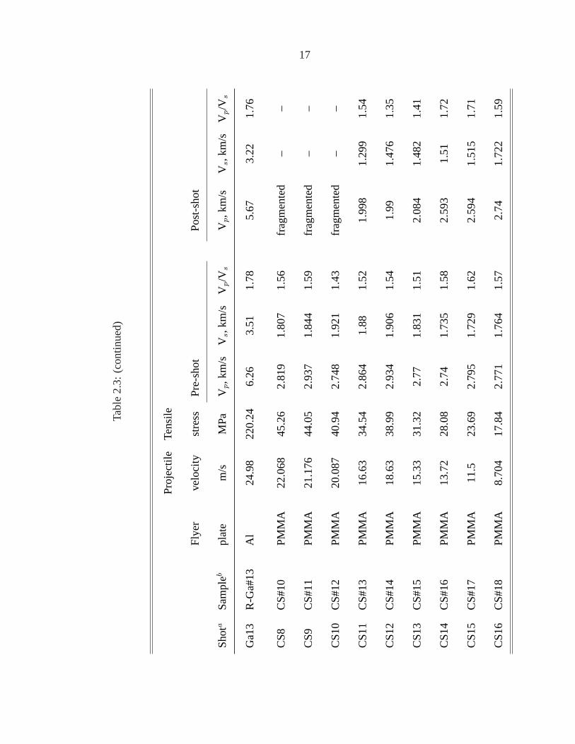
2.4 Results and discussion

Figure 2.2 shows the spall cracks observed in the recovered samples. Both pre-shot and

post-shot ultrasonic compressional and shear wave velocities in the direction perpendicular

to the impact surface, andVp/Vs are listed in Table 2.4, as well as impact velocities and

relative tensile stresses for our experiments. Figure 2.3 to 2.6 show velocity reductions

with tensile stresses for the four types of rocks and Figure 2.8 isVp/Vs ratio versus tensile

stresses. Several important effects are identified below:

14

1 cm

Spall cracksRadial cracks

(a)

(b)

Figure 2.2: Recovered samples: a) CS 27; b) One fragment of SE 5 to show the radial andspall (subhorizontal) cracks observed. The measured velocity reduction of (a) was∼36%and∼40% for P and S wave velocities. The velocity reduction for (b) was unmeasurable.

15

Tabl

e2.

3:O

ne-d

imen

sion

alte

nsile

stra

inim

pact

para

me-

ters

and

pre-

shot

and

post

-sho

tultr

ason

icco

mpr

essi

onal

and

shea

rve

loci

ties.

Pro

ject

ileTe

nsile

Fly

erve

loci

tyst

ress

Pre

-sho

tP

ost-

shot

Sho

taS

ampl

ebpl

ate

m/s

MP

aV p

,km

/sV s

,km

/sV p

/Vs

Vp,k

m/s

V s,k

m/s

V p/V

s

G23

SM

G#2

1A

l15

.62

147.

276.

908

3.53

81.

956.

434

3.51

91.

83

G24

SM

G#2

2A

l16

.97

159.

616.

833

3.64

71.

876.

524

3.53

81.

84

G26

SM

G#2

5A

l25

.19

227.

696.

533

3.47

91.

886.

053.

347

1.81

G28

SM

G#2

8A

l27

.89

253.

666.

427

3.49

61.

844.

936

3.15

61.

56

G29

SM

G#2

9A

l28

.53

272.

437.

137

4.68

31.

52fr

agm

ente

d–

–

G30

SM

G#3

0A

l23

.78

222.

586.

843.

618

1.89

5.9

3.33

71.

77

G31

SM

G#3

1A

l32

.11

297.

156.

687

3.50

61.

91fr

agm

ente

d–

–

G32

SM

G#3

2A

l26

.61

247.

076.

727

3.60

91.

865.

588

3.38

1.65

16

Tabl

e2.

3:(c

ontin

ued)

Pro

ject

ileTe

nsile

Fly

erve

loci

tyst

ress

Pre

-sho

tP

ost-

shot

Sho

taS

ampl

ebpl

ate

m/s

MP

aV p

,km

/sV s

,km

/sV p

/Vs

Vp,k

m/s

V s,k

m/s

V p/V

s

G34

SM

G#3

4A

l20

.118

4.7

6.52

63.

474

1.88

6.01

73.

379

1.78

G35

SM

G#2

4A

l13

.74

125.

896.

483

3.50

91.

856.

483

3.50

91.

85

Ga1

R-G

a#1

Al

1917

2.01

6.6

3.38

1.95

5.67

3.33

1.7

Ga3

R-G

a#3

Al

29.9

327

1.09

6.64

3.65

1.82

frag

men

ted

––

Ga5

R-G

a#5

Al

27.8

524

2.5

6.11

3.45

1.77

4.79

3.0

1.6

Ga7

R-G

a#7

Al

15.5

713

9.78

6.5

3.5

1.85

5.61

3.41

1.65

Ga8

R-G

a#8

Al

27.0

623

7.22

6.2

3.6

1.72

4.95

3.09

1.6

Ga9

R-G

a#9

Al

22.6

619

9.68

6.25

3.52

1.77

5.59

3.22

1.74

Ga1

1R

-Ga#

11A

l13

.47

120.

796.

453.

661.

756.

493.

471.

87

Ga1

2R

-Ga#

12A

l16

.37

146.

336.

463.

621.

796.

213.

441.

81

17

Tabl

e2.

3:(c

ontin

ued)

Pro

ject

ileTe

nsile

Fly

erve

loci

tyst

ress

Pre

-sho

tP

ost-

shot

Sho

taS

ampl

ebpl

ate

m/s

MP

aV p

,km

/sV s

,km

/sV p

/Vs

Vp,k

m/s

V s,k

m/s

V p/V

s

Ga1

3R

-Ga#

13A

l24

.98

220.

246.

263.

511.

785.

673.

221.

76

CS

8C

S#1

0P

MM

A22

.068

45.2

62.

819

1.80

71.

56fr

agm

ente

d–

–

CS

9C

S#1

1P

MM

A21

.176

44.0

52.

937

1.84

41.

59fr

agm

ente

d–

–

CS

10C

S#1

2P

MM

A20

.087

40.9

42.

748

1.92

11.

43fr

agm

ente

d–

–

CS

11C

S#1

3P

MM

A16

.63

34.5

42.

864

1.88

1.52

1.99

81.

299

1.54

CS

12C

S#1

4P

MM

A18

.63

38.9

92.

934

1.90

61.

541.

991.

476

1.35

CS

13C

S#1

5P

MM

A15

.33

31.3

22.

771.

831

1.51

2.08

41.

482

1.41

CS

14C

S#1

6P

MM

A13

.72

28.0

82.

741.

735

1.58

2.59

31.

511.

72

CS

15C

S#1

7P

MM

A11

.523

.69

2.79

51.

729

1.62

2.59

41.

515

1.71

CS

16C

S#1

8P

MM

A8.

704

17.8

42.

771

1.76

41.

572.

741.

722

1.59

18

Tabl

e2.

3:(c

ontin

ued)

Pro

ject

ileTe

nsile

Fly

erve

loci

tyst

ress

Pre

-sho

tP

ost-

shot

Sho

taS

ampl

ebpl

ate

m/s

MP

aV p

,km

/sV s

,km

/sV p

/Vs

Vp,k

m/s

V s,k

m/s

V p/V

s

CS

17C

S#1

9P

MM

A6.

413

13.1

92.

81.

777

1.58

2.8

1.77

71.

58

CS

18C

S#2

0P

MM

A19

.28

39.9

32.

809

1.86

1.51

frag

men

ted

––

CS

19C

S#2

1P

MM

A14

.923

30.5

52.

781.

783

1.56

1.84

11.

231.

5

CS

20C

S#2

2P

MM

A18

.476

38.6

2.90

71.

873

1.55

frag

men

ted

––

CS

21C

S#2

3P

MM

A11

.828

23.9

2.70

31.

769

1.53

2.38

1.58

51.

5

CS

22C

S#2

4P

MM

A7.

688

15.8

42.

813

1.80

71.

562.

813

1.57

61.

78

CS

23C

S#2

5P

MM

A9.

984

20.3

42.

744

1.69

31.

622.

644

1.53

51.

72

CS

24C

S#2

6P

MM

A13

.729

28.3

22.

831

1.88

1.51

2.35

91.

523

1.55

CS

25C

S#2

7P

MM

A16

.357

33.7

62.

838

1.83

21.

552.

189

1.35

1.62

CS

26C

S#2

8P

MM

A16

32.8

2.76

61.

796

1.54

2.02

31.

352

1.5

19

Tabl

e2.

3:(c

ontin

ued)

Pro

ject

ileTe

nsile

Fly

erve

loci

tyst

ress

Pre

-sho

tP

ost-

shot

Sho

taS

ampl

ebpl

ate

m/s

MP

aV p

,km

/sV s

,km

/sV p

/Vs

Vp,k

m/s

V s,k

m/s

V p/V

s

CS

27C

S#2

9P

MM

A16

.709

34.6

72.

855

1.84

51.

551.

826

1.11

1.65

CS

28C

S#3

0P

MM

A15

.075

30.9

82.

768

1.87

71.

472.

206

1.44

31.

53

SE

1S

E#1

Al

60.0

7757

8.12

6.09

63.

811.

6fr

agm

ente

d–

–

SE

2S

E#2

Al

48.9

347

1.34

6.08

33.

883

1.57

3.13

92.

511.

25

SE

3S

E#3

Al

42.2

140

8.76

6.16

53.

909

1.58

4.39

13.

091.

42

SE

4S

E#4

Al

33.2

2634

0.7

7.00

83.

976

1.76

5.69

3.72

51.

53

SE

5S

E#5

Al

55.7

7154

7.56

6.32

93.

836

1.65

frag

men

ted

––

SE

6S

E#6

Al

24.1

244.

866.

993.

888

1.8

6.28

43.

736

1.68

SE

7S

E#7

Al

38.0

6837

2.15

6.48

63.

884

1.67

4.14

33.

144

1.32

SE

8S

E#9

Al

28.3

9628

3.16

6.57

43.

61.

835.

361

3.01

71.

78

20

Tabl

e2.

3:(c

ontin

ued)

Pro

ject

ileTe

nsile

Fly

erve

loci

tyst

ress

Pre

-sho

tP

ost-

shot

Sho

taS

ampl

ebpl

ate

m/s

MP

aV p

,km

/sV s

,km

/sV p

/Vs

Vp,k

m/s

V s,k

m/s

V p/V

s

SE

9S

E#1

0A

l45

.92

430.

555.

855

3.38

91.

733.

231

2.38

1.36

SE

10S

E#1

1A

l30

.138

286.

376.

047

3.45

1.75

5.02

32.

917

1.72

SE

11S

E#8

Al

24.7

924

6.86

6.77

13.

934

1.72

03.

530

aD

urat

ion

time

is∼

1µ

sfo

rG

23to

Ga1

3,S

E1

toS

E11

;∼2.

4µ

sfo

rC

S8

toC

S17

;∼1.

4µ

sfo

rC

S18

toC

S28

.bS

MG

:San

Mar

cos

gabb

ro;G

a:S

anM

arco

sgr

anite

;CS

:Coc

onin

osa

ndst

one;

SE

:Ses

iaec

logi

te.

21

100 150 200 250 300

0

10

20

30

Computed tensile stress (MPa)

Sou

nd v

eloc

ity r

educ

tion

(%)

Al flyer plates, 1 µs duration

→

Completefragmentation

Onset of tensileFailure

P−waveS−wavefractured

Figure 2.3: Velocity measurements for San Marcos gabbro experiments. Dashed line indi-cates pressure above which complete fragmentation occurred.

1. P- and S-wave velocity reductions occur with increasing tensile stress for the four

types of rocks studied (Figures 2.3 to 2.6). The highest P-wave velocity reduction

measured is 27-30% for San Marcos gabbro and granite, and 10-15% for S-wave

velocity (Figure2.3, 2.4). For Sesia eclogite measurements, the results are 48% and

35% for P- and S-wave reduction, respectively (Figure 2.5). In the Coconino sand-

stone experiment with 2.4µs duration time, 30% and 25% are obtained for P- and

S-wave reduction, respectively, which increases to 36% and 40% for the 1.4µs du-

ration time case (Figure2.6a, b).

2. Figure 2.3 suggests that the onset of tensile failure of San Marcos gabbro determined

22

100 150 200 250 300

0

10

20

30

Computed tensile stress (MPa)

Sou

nd v

eloc

ity r

educ

tion

(%)

Al flyer plates, 1 µs duration

Onset of tensileFailure

→Completefragmentation

P−waveS−wavefractured

Figure 2.4: Velocity measurements for San Marcos granite experiments. Dashed line indi-cates pressure above which complete fragmentation occurred.

by the detectable ultrasonic velocity reduction is∼ 150 MPa. This result is compa-

rable with a previous microscopic examination of recovered samples [Lange et al.,

1984]. Within this range,Lange et al.[1984] reported that incipient cracks, more or

less continuous, were observed. This also validates the ultrasonic method for deter-

mining dynamic tensile strength. Complete fragmentation occurs above 250 MPa.

This is determined to be the fracture strength.

3. Onset of tensile failure of San Marcos granite is∼ 130 MPa (Figure 2.4). Complete

fragmentation occurs above 250 MPa, very close to that of San Marcos gabbro.

4. The onset of tensile failure for Sesia eclogite is∼ 240 MPa. This is the highest

23

200 300 400 500 600

0

20

40

50

Computed tensile stress (MPa)

Sou

nd V

eloc

ity r

educ

tion

(%)

Al flyer plates, 1 µs duration

macroscopicradial cracks→

→

Completefragmentation

Onset of tensileFailure

P−waveS−wavefractured

Figure 2.5: Velocity measurements for Sesia eclogite experiments. Dashed lines indicatepressure above which macroscopic radial and complete fragmentation occurred.

known limit of tensile strength measured by experiment for terrestrial rocks. The

observable continuous cracks for Sesia eclogite appear around tensile stress about

400 MPa (Figure2.5). Complete fragmentation occurs above∼ 500 MPa.

5. The onset of tensile failure for Coconino sandstone, determined from detectable ul-

trasonic velocity reduction, is∼ 17 MPa for the 2.4µs shock duration time, and∼

20 MPa for the 1.4µs duration time. Macroscopic radial cracks appear at∼ 30 MPa

and complete fragmentation at∼ 40 MPa for both cases (Figure 2.6).

6. The reduction of P-wave velocity is greater than the reduction of S-wave velocity for

both San Marcos gabbro (Figure 2.3) and Sesia eclogite (Figure 2.5). There is no

24

10 20 30 40 50

0

20

40

Computed tensile stress (MPa)

Sou

nd v

eloc

ity r

educ

tion

(%)

Coconino sandstone, ~2.4 µs duration

macroscopicradial cracks

→

→

Completefragmentation

Onset of tensile

Failure

(a)

P−waveS−wavefractured

(a)

10 20 30 40 50

0

20

40

Computed tensile stress (MPa)

Sou

nd v

eloc

ity r

educ

tion

(%)

Coconino sandstone, ~1.4 µs duration

macroscopicradial cracks

→

→

Completefragmentation

Onset of tensile

Failure

(b)

P−waveS−wavefractured

(b)

Figure 2.6: Velocity measurements for Coconino sandstone experiments of duration timeof (a) 2.4µs and (b) 1.4µs. Dashed lines indicate the same as those in Figure 2.5.

25

Figure 2.7: Velocity measurements for Bedford limestone. (a) 0.5µs and (b) 1.3µs. (FromAhrens and Rubin[1993], Fig. 2.)

26

obvious relation between P- and S-wave reduction for Coconino sandstone.

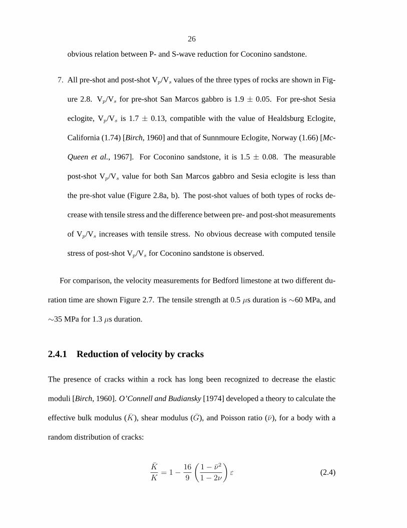
7. All pre-shot and post-shot Vp/Vs values of the three types of rocks are shown in Fig-

ure 2.8. Vp/Vs for pre-shot San Marcos gabbro is 1.9± 0.05. For pre-shot Sesia

eclogite, Vp/Vs is 1.7± 0.13, compatible with the value of Healdsburg Eclogite,

California (1.74) [Birch, 1960] and that of Sunnmoure Eclogite, Norway (1.66) [Mc-

Queen et al., 1967]. For Coconino sandstone, it is 1.5± 0.08. The measurable

post-shot Vp/Vs value for both San Marcos gabbro and Sesia eclogite is less than

the pre-shot value (Figure 2.8a, b). The post-shot values of both types of rocks de-

crease with tensile stress and the difference between pre- and post-shot measurements

of Vp/Vs increases with tensile stress. No obvious decrease with computed tensile

stress of post-shot Vp/Vs for Coconino sandstone is observed.

For comparison, the velocity measurements for Bedford limestone at two different du-

ration time are shown Figure 2.7. The tensile strength at 0.5µs duration is∼60 MPa, and

∼35 MPa for 1.3µs duration.

2.4.1 Reduction of velocity by cracks

The presence of cracks within a rock has long been recognized to decrease the elastic

moduli [Birch, 1960].O’Connell and Budiansky[1974] developed a theory to calculate the

effective bulk modulus (K), shear modulus (G), and Poisson ratio (ν), for a body with a

random distribution of cracks:

K

K= 1− 16

9

(1− ν2

1− 2ν

)ε (2.4)

27

G

G= 1− 32

45

(1− ν) (5− ν)

2− νε (2.5)

ν = ν

(1− 16

9ε

)(2.6)

whereK is bulk modulus,G is shear modulus,ν is Poisson ratio of the undamaged

body, andε is crack density. From equations above, a crack density of 0.05 would produce

∼ 4% P-wave reduction and∼ 1.5% S-wave reduction.

100 150 200 250 3001.5

1.6

1.7

1.8

1.9

2(a)

Vp/V

s

200 300 400 5001

1.2

1.4

1.6

1.8

2(b)

10 20 30 401.3

1.4

1.5

1.6

1.7

1.8(c)

tensile stress (MPa)

Vp/V

s

10 20 30 401.3

1.4

1.5

1.6

1.7

1.8(d)

tensile stress (MPa)

Figure 2.8: Post-shotVp/Vs values versus computed tensile stress: a) San Marcos gabbro(SMG); b) Sesia eclogite (SE); c) Coconino sandstone (CE) with 2.4µs duration time; d)sandstone with 1.4µs duration time. Open squares are average pre-shotVp/Vs: 1.87 forSMG, 1.7 for SE, and 1.54 for CS. Error bars represent lower and upper limits of pre-shotVp/Vs value. Stars are post-shotVp/Vs values. Straight lines in (a) and (b) are linear fit ofpost-shot results for SMG and SE. Post-shotVp/Vs decreases with computed tensile stressfor both cases. Post-shotVp/Vs values of CS for two duration time cases are scattered. Noobvious relation between post-shotVp/Vs and tensile stress observed for CS.

28

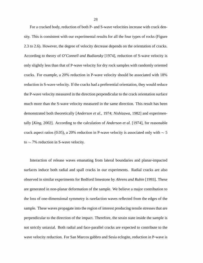
For a cracked body, reduction of both P- and S-wave velocities increase with crack den-

sity. This is consistent with our experimental results for all the four types of rocks (Figure

2.3 to 2.6). However, the degree of velocity decrease depends on the orientation of cracks.

According to theory ofO’Connell and Budiansky[1974], reduction of S-wave velocity is

only slightly less than that of P-wave velocity for dry rock samples with randomly oriented

cracks. For example, a 20% reduction in P-wave velocity should be associated with 18%

reduction in S-wave velocity. If the cracks had a preferential orientation, they would reduce

the P-wave velocity measured in the direction perpendicular to the crack orientation surface

much more than the S-wave velocity measured in the same direction. This result has been

demonstrated both theoretically [Anderson et al., 1974;Nishizawa, 1982] and experimen-

tally [King, 2002]. According to the calculation ofAnderson et al.[1974], for reasonable

crack aspect ratios (0.05), a 20% reduction in P-wave velocity is associated only with∼ 5

to∼ 7% reduction in S-wave velocity.

Interaction of release waves emanating from lateral boundaries and planar-impacted

surfaces induce both radial and spall cracks in our experiments. Radial cracks are also

observed in similar experiments for Bedford limestone byAhrens and Rubin[1993]. These

are generated in non-planar deformation of the sample. We believe a major contribution to

the loss of one-dimensional symmetry is rarefaction waves reflected from the edges of the

sample. These waves propagate into the region of interest producing tensile stresses that are

perpendicular to the direction of the impact. Therefore, the strain state inside the sample is

not strictly uniaxial. Both radial and face-parallel cracks are expected to contribute to the

wave velocity reduction. For San Marcos gabbro and Sesia eclogite, reduction in P-wave is

29

greater than that of S-wave velocity, indicating that the major contribution comes from the

face-parallel cracks. No obvious pattern was observed for Coconino sandstone.

Although we can determine the elastic wave velocity from a given crack distribution, the

converse is not true. It is impossible to determine the exact crack distribution in rocks just

from elastic wave velocity measurements, since the distribution of cracks is not a unique

function of the velocities [Nur, 1971]. Further experiments are under way to study the

different contributions to velocity reductions of different oriented cracks.

2.4.2 Interpretation of Vp/Vs

Since shear wave velocity is less sensitive than the compressional wave velocity to the

presence of cracks normal to the propagation direction of the wave [Nur, 1971;Anderson

et al., 1974], we can use Vp/Vs to illuminate the orientation of cracks for the three types

of rocks. The average pre-shot Vp/Vs is ∼1.9 for San Marcos gabbro (Figure 2.8a) and

∼1.7 for Sesia eclogite (Figure 2.8b). The post-shot Vp/Vs for both types of rocks are less

than the pre-shot value, indicating the cracks produced by the shock were mainly oriented

parallel to the impact surfaces. The post-shot Vp/Vs for both types of rocks decrease with

increasing computed tensile stress, which means higher crack density. There is no good

reason for the random pattern of post-shot Vp/Vs for Coconino sandstone (Figure 2.8c, d).

Further work should be conducted to study the anisotropy of sandstone.

30

2.4.3 Strain-rate effect

It has long been recognized in fracture mechanics that strength of material depends on

the rate at which the loading is applied. Dynamic tensile strength of rocks at high strain

rates produced by shock wave interactions can exceed the quasi-static tensile strength by an

order of magnitude [Grady and Hollenbach, 1979]. Cohn and Ahrens[1981] came to the

similar conclusion in their studies of analogues of lunar rocks. Similar behavior has been

observed for ice-silicate mixtures [Lange and Ahrens, 1983]. Grady and Lipkin[1980]

have generalized a wide range of data suggesting dependence of tensile fracture strength

on strain rate.Grady [1998] gives the strain rate dependent criteria of tensile strength (σt)

for ceramics:

σt =(6ρ2c3ε

)1/3(2.7)

Wherec is the compressional wave velocity,ρ is the density andε is the strain rate, defined

as:

ε =ε

∆t(2.8)

ε is strain, and∆t is the duration time.Lange and Ahrens[1983] giveε as a function of

known material material parameters:

ε =ρiVi

ρiVi + ρtVt

Up

Vt

(2.9)

Generally, the tensile strength is proportional to a power of the strain rate, with the

power law exponent typically around 1/4 to 1/3, depending on the materials [Grady and

Lipkin, 1980;Housen and Holsapple, 1990;Grady, 1998].

31

The porous Coconino sandstone is expected to behave differently from the ceramics.

However, the assumption is still valid that the dynamic tensile strength is proportional to a

power of the strain rate. Taken our experiment results of 20 MPa at 1.4µs duration time

and 17 MPa at 2.4µs duration time, the power law exponent is calculated to be 1/3.3 for

Coconino sandstone. The strain,ε, is assumed to be the same for the two duration time

experiments. The power law exponent fits very well within the range of previous study, 1/4

to 1/3 [Grady and Lipkin, 1980].

Table 2.4: Tensile strengths (in MPa) of ice and rocks at different strain rates.Strain rate (106s−1)10−6 2x10−2 1/2.4 1/1.4 1/1.3 1 1/0.5 σc

a

Coconino sandstone - - 17(1) 20(1) - - - -Bedford limestone - - - - 35(2) - 60(2) 40b

Ice 1.6(3) 17(3) - - - - - 40b

San Marcos gabbro - - - - - 150(1) - 150c

Sources: (1)This study; (2)Ahrens and Rubin[1993]; (3)Lange et al.[1984].aDynamic tensile strength at strain rate of 106 s−1.bExtrapolated from available data.cMeasured.

The tensile strengths of ice and different rocks at different strain rates are given in Table

2.4. Also included isσc, the tensile strength at a strain rate of106s−1, extrapolated from

available data or measured directly. The dynamic tensile strengths of Coconino sandstone,

normalized byσc, versus strain rate are plotted in Figure 2.9. Also included in Figure 2.9

are the dynamic tensile strength of ice and Bedford limestone data from previous work

[Lange and Ahrens, 1983;Ahrens and Rubin, 1993]. Non-linear square fit for all these data

by the relation ofσ/σc = aε1b gives a = 0.03±0.02, b = 3.97±0.05.

The tensile strength has a strong dependent on strain rate in the high strain rate region.

Care must be taken when applying the experimental measurement of sandstone to field

32

10−1

101

103

105

107

10−1

100

strain rate, s−1

Nor

mal

ized

tens

ile s

tren

gth

Ice (Lange et al, 1983)Coconino Sandstone, this study Bedford limestone, (Ahrens & Rubin, 1993)San Marcos gabbro (Lange et al., 1984)

Figure 2.9: Normalized tensile strengths as a function of strain rate for ice and rocks.Dashed line is a non-linear square fit ofσ/σc = aε1/b to available data. Note log scalehere. See text for detailed explanation.

impact crater, for which the strain rate is about three orders of magnitude lower, or, the

duration time is about three orders of magnitude longer, than that in the experiments.

2.5 Conclusion

Four types of terrestrial rocks, San Marcos gabbro and granite, Coconino sandstone, and

Sesia eclogite were subject to planar impacts to produce tensile failure under dynamic

loading conditions. Two sets of experiments with different duration times were conducted

for porous sandstone. Ultrasonic velocity measurements of pre-shot and post-shot samples

were measured to determine the dynamic tensile strength and the fracture strength of each

type of rock by detectable velocity reduction. Major results are:

1. The onset of cracking occurs at∼ 150 MPa for San Marcos gabbro,∼ 130 MPa for

33

San Marcos granite,∼ 20 MPa for Coconino sandstone at 1.4µs duration,∼17 MPa

at 2.4µs duration, and 240 MPa for Sesia eclogite. Complete fracture occurs above

250 MPa for gabbro and granite, 40 MPa for sandstone, and∼ 480 MPa for eclogite.

2. Both reductions of P- and S-wave reduction for all the four types of rocks increase

with the computed tensile stress, indicating the higher tensile pressure produced

higher crack density.Vp/Vs of post-shot San Marcos gabbro and Sesia eclogite sam-

ples decrease with the computed tensile pressure. No obvious relation between post-

shotVp/Vs of Coconino sandstone and the computed tensile pressure is observed.

3. Higher reduction of P-wave than S-wave velocity in San Marcos gabbro, granite and

Sesia eclogite indicates that spall (subparallel to the impact surface) cracks contribute

more to the velocity reduction than radial cracks. Random pattern of reductions of P-

and S-wave velocity for Coconino sandstone is possibly caused by its high porosity

and variety between separate samples.Vp/Vs of post-shot San Marcos gabbro and

Sesia eclogite samples are less than the pre-shot values.

Acknowledgments:We appreciate the technical support of E. Gelle, M. Long, and the

advice of Professor G. Ravichandran. The paper benefited from the helpful comments of

K. Housen and E. Pierazzo.

34

Chapter 3

Tomography Study of Shock-InducedDamage beneath Craters

3.1 Introduction

This study improved and extended the tomography method used inXia and Ahrens[2001]

to map the damage zones beneath impact craters using the non-destructive tomography

method. First we will discuss the tomography experimental setup for mapping the velocity

profile. A detailed description of the tomography method used for velocity profile inversion

is given next. Using the tomography method, the P-wave structure of the center plane for

the recovered San Marcos granite after impact by a lead bullet at velocity of 1200 m/s is

inverted and compared with the cut-open cross-section result.

35

3.2 Experimental procedure

3.2.1 Cratering

Initially, 20x20x15 cm blocks were cut from San Marcos granite. The parallelism of two

parallel surfaces is± 0.5 mm, and one surface is polished to be the impact surface. All the

surfaces are smooth enough to get good coupling between the transducers and target for

ultrasonic measurement. The granite target is impacted by a lead bullet with diameter of

0.6 mm and mass of 3.2 g at impact velocity of∼ 1.2 km/s at normal impact angle. The

impact velocity is chosen such that the damage produced in the target is moderate for the

dimension of the target (i.e., neither too severe to fragment the whole target, nor too weak

to produce measurable compressional velocity reduction using the tomography method).

3.2.2 Tomography technique

Figure 3.1 shows the experimental setup for the tomography measurement. To gener-

ate a strong hemispherical instead of beam-like ultrasonic wave which could penetrate

the damaged low-velocity crater zone, mechanical source instead of transducer source is

used. A 0.08 cm diameter stainless steel sphere, positioned on a weak tape, is launched

by pre-compressed gas to produce the source wave (Figure 3.1b). The pressure of the pre-

compressed gas is approximately 400 KPa for each shot. The release of the pre-compressed

gas is controlled by a solenoid operated valve. The impact velocity of the ball onto the

target surface is not measurable using the present technique, but the travel time of the ul-

trasonic wave should be dependent mostly on the media to be measured, and not on the

36

(a)

(b)

Figure 3.1: (a) Cross section of tomography measurement setup; (b) Enlarged side view ofposition of 0.08 cm diameter steel impactor sphere.

37

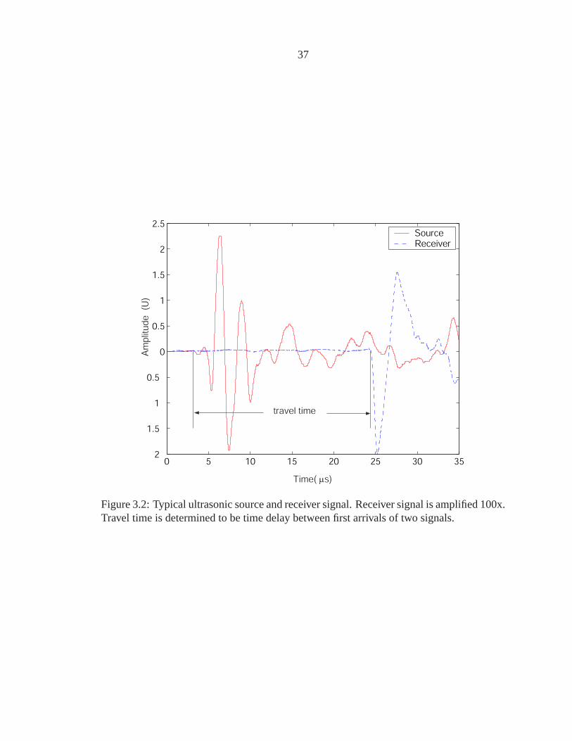
0 5 10 15 20 25 30 352

1.5

1

0.5

0

0.5

1

1.5

2

2.5

Time( s)

Amplitude (U

)

travel time

SourceReceiver

µ

Figure 3.2: Typical ultrasonic source and receiver signal. Receiver signal is amplified 100x.Travel time is determined to be time delay between first arrivals of two signals.

38

impact velocity of the impactor ball. Tests show that the travel time measured in this way

is quite repeatable. To prevent formation of micro-craters by the impact of the steel ball,

A 0.05 cm thick tungsten carbide (WC) plate is placed on the target surface at the impact

point (Figure 3.1a).

Two P-wave piezoelectric transducers (Model 1191, Panametrics, central frequency 5

MHz) are used to determine the travel time of each ray. The two transducers are positioned

in the holder plates. To make good contact between the measured target surface and the

transducers, the two holder plates are tightened by a tightening ”C” clip (Figure 3.1a). One

transducer is placed close to the impact point, with distance of 0.5 cm, to be the impact

source. The error of travel time measurement caused by this is neglectable considering the

dimension of the target block. A typical record is shown in Figure 3.2 and the travel time

is determined by the time delay between the initial jumps of the two signals. Uncertainty

in time measurement is± 0.05µs.

The compressional wave velocity of the center plane (15x20 cm) of a San Marcos gran-

ite block is mapped using the tomography setup described above to check the heterogeneity

of the sample. Figure 3.3 is diagram showing the sources and relative recording stations

along the center plane of the pre-shot granite target assuming straight ray path for the sur-

vey. Grid used for tomography inversion is one centimeter. Cells are numbered from left

to right, top to bottom. The index of thejth cell of ith row is therefore20x(i-1)+j. Index

of a few cells are shown in Figure 3.3. Source and the second transducer are first placed on

the two parallel surfaces (left and right, top and bottom) of the target. Then on the top side

of the granite, four sources are deployed, each of which has detection stations/receivers on

39

0 5 10 15 20

0

5

10

15

cm

cm

S1 S2 S3 S4

Cell

1

Cell

181

Cell

20

Cell

200

Figure 3.3: Tomographic straight ray diagram for pre-shot San Marcos granite. Thickdashed lines are cell boundaries and thin dashed lines tomographic rays. Index of cellsare increased from left to right, top to bottom. Forjth cell in ith row, index is 20x(i-1)+j.Cell 1, 20, 180 and 200 are numbered. Sources placed at S1, S2, S3 and S4, and receiverstations on bottom and side surface across to fully cover target. Shot is numbered withindex of source and receiver. For S1 and S2, index of receiver increases from 1 to 20 onbottom side, and 21 to 35 on side surface across. For example, shot 106 represents sourceS1 and receiver 6, which is sixth cell on bottom side. For S3 and S4, index of receiverstarts reversely. 0.05 cm thick tungsten carbide plate is placed at impact point to preventmicro-crater formed in rock.

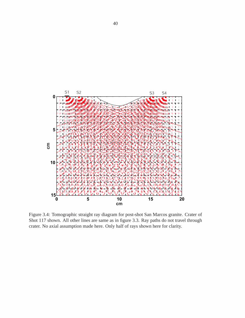
40

0 5 10 15 20

0

5

10

15

cm

cm

S1 S2 S3 S4

Figure 3.4: Tomographic straight ray diagram for post-shot San Marcos granite. Crater ofShot 117 shown. All other lines are same as in figure 3.3. Ray paths do not travel throughcrater. No axial assumption made here. Only half of rays shown here for clarity.

41

the bottom and the side surface across, to fully cover the center plane. The data obtained

from the top sources measurement are mirrored based on the axial symmetry assumption.

The seismic survey distribution for the recovered granite target after impact is different

from that of pre-shot in that the rays passing through the heavily damaged zone beneath the

crater are not taken into account, since the amplitudes of these rays are attenuated greatly

and no readable signal could be obtained (Figure 3.4). No assumption of axial symmetry

is made for the shock-induced damage in the recovered granite target. Therefore, eight

sources, instead of four, on the top surface of the rock block, are deployed to get a full

coverage of the interested area. Overall, 264 (8x33) data points are obtained from these top

surface sources measurements.

3.3 Results and discussion

3.3.1 Tomography inversion

Tomography means ’representation in cross-section’ and is first used in medical diagnosis.

Seismic tomography uses the same principles as that of x-rays, with the difference that the

travel times of the signals, rather than the attenuation, are observed. Travel times from an

earthquake source are inverted to obtain information about the seismic velocity structure of

the earth. For our study, the compressional wave velocity of one central plane (15x20 cm

in dimension) of the granite target is mapped using the tomography setup described above.

The cell size is 1 cm, thus 300 cells (model parameters) are used for inversion. Assuming

the plane is divided intoN cells (N is 300 for this case), and there areM rays recorded from

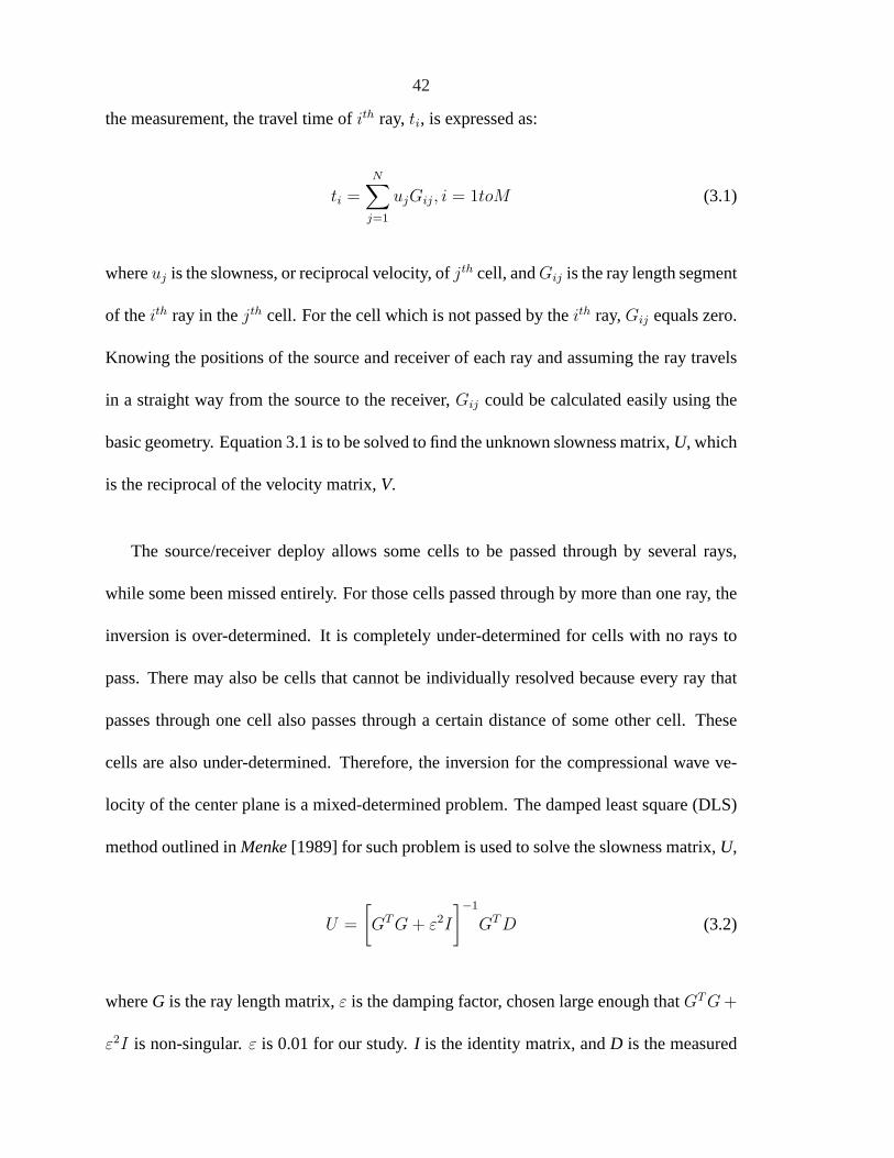
42

the measurement, the travel time ofith ray, ti, is expressed as:

ti =N∑

j=1

ujGij, i = 1toM (3.1)

whereuj is the slowness, or reciprocal velocity, ofjth cell, andGij is the ray length segment

of theith ray in thejth cell. For the cell which is not passed by theith ray,Gij equals zero.

Knowing the positions of the source and receiver of each ray and assuming the ray travels

in a straight way from the source to the receiver,Gij could be calculated easily using the

basic geometry. Equation 3.1 is to be solved to find the unknown slowness matrix,U, which

is the reciprocal of the velocity matrix,V.

The source/receiver deploy allows some cells to be passed through by several rays,

while some been missed entirely. For those cells passed through by more than one ray, the

inversion is over-determined. It is completely under-determined for cells with no rays to

pass. There may also be cells that cannot be individually resolved because every ray that

passes through one cell also passes through a certain distance of some other cell. These

cells are also under-determined. Therefore, the inversion for the compressional wave ve-

locity of the center plane is a mixed-determined problem. The damped least square (DLS)

method outlined inMenke[1989] for such problem is used to solve the slowness matrix,U,

U =

[GT G + ε2I

]−1

GT D (3.2)

whereG is the ray length matrix,ε is the damping factor, chosen large enough thatGT G +

ε2I is non-singular.ε is 0.01 for our study.I is the identity matrix, andD is the measured

43

travel time data matrix.

The agreement between the estimated and the true model parameters is evaluated by

the model resolution matrix,R, defined as:

R =

[GT G + ε2I

]−1

GT G (3.3)

3.3.2 Test problems

Two test problems are carried out to validate the tomography method developed above.

First, a 20x15 cm block with homogenous velocity structure, which is the simplest situa-

tion, is tested. Figure 3.5a shows the homogenous velocity structure for forward modelling.

The velocity is 6.4 km/s. Synthetic travel times from sources to receivers deployed in Fig-

ure 3.3 are calculated using the high-resolution finite difference package ofHole [1992],

originated fromVidale [1990], which allows calculation of the travel time field in three

dimensions for a given velocity model. These synthetic travel time data are used as input

into the tomography inversion, and Figure 3.5b shows the inverted velocity structure with

the straight ray assumption. It is obvious that the cm-scale tomography method works very

well for the structure without obvious velocity contrast.

The second test carried out is a 20x15 cm block with a low velocity zone of 5 km/s in

the middle and 6.4 km/s for the rest (Figure 3.6a). The same tomography method is applied

to get the inverted velocity structure, using the straight ray assumption.

For relatively homogenous velocity structure, the straight ray path assumption is valid.

However, if there are large velocity contrasts in the body to be studied, this assumption

44

might not be realistic and it is necessary to take into account the possibility of curve ray

path. Next we will discuss how to determine the real curve ray path in a structure with

velocity contrast.

There are several possible ways for a seismic wave to travel from point A to point B

within a large velocity contrast structure. Figure 3.9a shows two of these possible ways.

The travel times for the two rays are t1 and t2, with t1 > t2. P-wave first arrivals take a

minimum travel time from the source to the receiver, the real path is ray 2 instead of ray

1 in Figure 3.9a. This is also true if the wave travels backward from point B to point A

(Figure 3.9b). The signal will take the same ray path which requires the minimum travel

time, t2. Therefore, for a wave travelling from point A to B and then propagating back,

the actual ray path is the one with the minimum total travel time. Understanding this, it is

straightforward now to find out the real ray path in the heterogenous block studied.

To find the real curve ray path from one source (S) to one receiver (R), the travel time

from S to all the grid points is calculated using the 3-D finite differential package [Hole,

1992] and the velocity model obtained from straight ray assumption as the reference model.

To improve the resolution of the forward calculation, a forward model cell size of 0.5 cm

is used instead of 1 cm. Similarly, the travel time fromR to all the grid points is also

calculated. If we add the two travel time matrix together, the true curve ray path can be

found by joining those points which have the minimum values of travel time within each

column between the source and the receiver.

The other rays from all the sources to the receivers are found in the same way. The

new curve ray length matrixG, where terms are the lengths of theith ray in thejth cell,

45

7400

7000

6600

6200

5800

5400

cell index in x

cell

ind

ex

in y

inverted velocity (m/s)

5 10 15 20

2

4

6

8

10

12

14

(a)

7000

6500

6000

5500

5000

cell index in x

cell

index

in y

inverted velocity (m/s)

5 10 15 20

2

4

6

8

10

12

14

7400

(b)

Figure 3.5: Test of the cm-scale tomography method developed above using a homogenousvelocity structure. (a) Forward velocity model. Velocity of the 20x15 cm structure is6.4 km/s; (b) Inverted velocity structure using the tomography method with straight rayassumption.

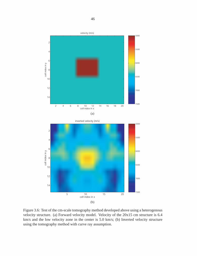
46

7500

7000

6500

6000

5500

5000

cell index in x

cell

ind

ex

in y

velocity (m/s)

2 4 6 8 10 12 14 16 18 20

2

4

6

8

10

12

14

(a)

7500

7000

6500

6000

5500

5000

cell index in x

cell

index

in y

inverted velocity (m/s)

5 10 15 20

2

4

6

8

10

12

14

(b)

Figure 3.6: Test of the cm-scale tomography method developed above using a heterogenousvelocity structure. (a) Forward velocity model. Velocity of the 20x15 cm structure is 6.4km/s and the low velocity zone in the center is 5.0 km/s; (b) Inverted velocity structureusing the tomography method with curve ray assumption.

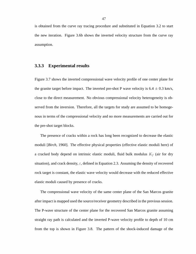
47

is obtained from the curve ray tracing procedure and substituted in Equation 3.2 to start

the new iteration. Figure 3.6b shows the inverted velocity structure from the curve ray

assumption.

3.3.3 Experimental results

Figure 3.7 shows the inverted compressional wave velocity profile of one center plane for

the granite target before impact. The inverted pre-shot P wave velocity is 6.4± 0.3 km/s,

close to the direct measurement. No obvious compressional velocity heterogeneity is ob-

served from the inversion. Therefore, all the targets for study are assumed to be homoge-

nous in terms of the compressional velocity and no more measurements are carried out for

the pre-shot target blocks.

The presence of cracks within a rock has long been recognized to decrease the elastic

moduli [Birch, 1960]. The effective physical properties (effective elastic moduli here) of

a cracked body depend on intrinsic elastic moduli, fluid bulk modulusKf (air for dry

situation), and crack density,ε, defined in Equation 2.3. Assuming the density of recovered

rock target is constant, the elastic wave velocity would decrease with the reduced effective

elastic moduli caused by presence of cracks.

The compressional wave velocity of the same center plane of the San Marcos granite

after impact is mapped used the source/receiver geometry described in the previous session.

The P-wave structure of the center plane for the recovered San Marcos granite assuming

straight ray path is calculated and the inverted P-wave velocity profile to depth of 10 cm

from the top is shown in Figure 3.8. The pattern of the shock-induced damage of the

48

8000

7500

7000

6500

6000

5500

5000

4500

cell index in x

ce

ll in

de

x in

y

5 10 15 20

2

4

6

8

10

12

14

m/s

Figure 3.7: Inversion solution of compressional wave velocity structure of pre-shot SanMarcos granite using straight ray deploy in Figure 3.3. A low pass filter was applied toinitial inverted result to get this profile.

recovered San Marcos granite, expressed as the compressional wave low velocity zone

here, is quite symmetric. This phenomenon confirms the axial symmetry assumption for

vertical impact problem. The reduction of the compressional wave velocity reaches∼ 40%

from the intrinsic value for the highly damaged region beneath and near the crater, 4 km/s

approximately. And the velocity increases with depth until the unshocked intrinsic value is

reached at depth of 7± 1 cm along the center line.

49

8000

7500

7000

6500

6000

5500

5000

4500

cell index in x

ce

ll in

dex in y

2 4 6 8 10 12 14 16 18 20

1

2

3

4

5

6

7

8

9

10

m/s

Figure 3.8: Compressional wave velocity structure of post-shot San Marcos granite of shotNo. 117 from top surface to depth of 10 cm using straight ray deploy described in Figure3.4. Same low pass filter as in Figure 3.7 was applied. Thick solid line defines crater. Lowvelocity zone extends to∼ 7 cm.

Figure 3.10a is the arrival travel time field from the source (S) to all the grid points

in the refined forward model calculated using the 3-D finite differential package [Hole,

1992]. Similarly, Figure 3.10b is the arrival travel time field to all the grid points with

source placed on the position of the receiver (R). The travel time from the source to itself

is, of course, zero, and increases with the distance from the source point, as shown in these

two figures. Figure 3.10c is the sum of the two travel time matrices from Figure 3.10a and

3.10b. The curve ray from the source to the receiver deflects from the straight ray path

slightly (Figure 3.10c).

Figure 3.11 shows a few samples of the curve rays from the source to receivers at

different positions using the velocity model inverted from straight ray path assumption.

Figure 3.12a compares the travel time from experimental measurements, the calculated

50

Figure 3.9: Diagram showing minimum travel time rule for a stress wave traveling betweenpoint A and point B. (a) Two possible rays with travel time t1 and t2 separately (t1 > t2)from A to B, actual ray path follows ray with travel time t2. (b) Same ray path is followedif stress wave travels from B to A in same material.

51

30

25

20

15

10

5

5 10 15 20

5

10

15

S sm

cell index in x

cell index in y

(a)

30

25

20

15

10

5

0

5 10 15 20

5

10

15

R

sm

cell index in x

cell index in y

(b)

Figure 3.10: (to be continued)

52

50

48

46

44

42

40

38

36

34

5 10 15 20

5

10

15

S

R

Sm

(c)

cell index in x

ce

ll in

de

x in

y

Figure 3.10: Diagram of procedure to obtain minimum time path from source (S) to receiver(R). (a) Travel time to each grid point from source, using finite difference package [Hole,1992] and velocity model (Figure 3.8). Cell dimension used is 0.5 cm; (b) Travel time toeach grid point from receiver; (c) Sum of travel times from (a) and (b). Equal to travel timefor minimum time stress wave propagating from S to R, and reflected back. Minimum timepath found by joining points with minimum values within S and R of travel time matrix(thick solid line). Dashed line defines approximate low velocity zone beneath crater.

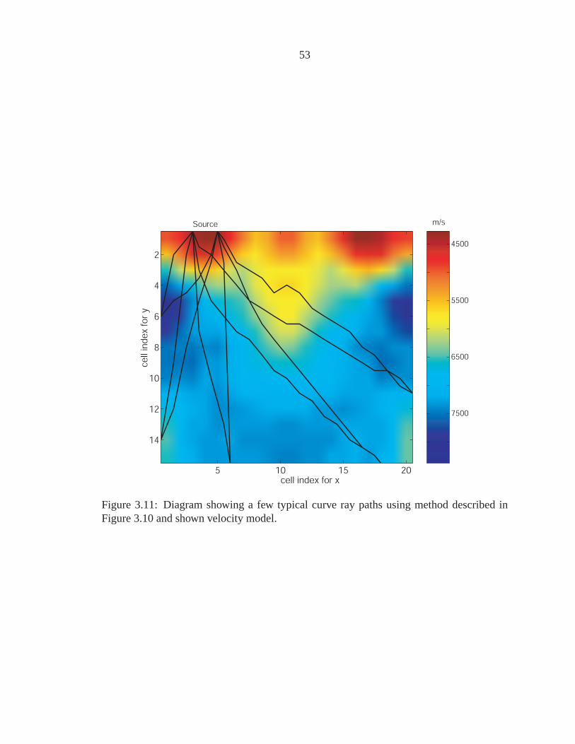
53

7500

6500

5500

4500

cell index for x

cell

index

for y

5 10 15 20

2

4

6

8

10

12

14

Source m/s

Figure 3.11: Diagram showing a few typical curve ray paths using method described inFigure 3.10 and shown velocity model.

54

100 150 200 250 300 350 400 45020

25

30

35

40

45

50tr

ave

l tim

e, (m

s)

experimentalmodeled,curvepathmodeled,straight line

100 150 200 250 300 350 400 45030

20

10

0

10

20

30

shot number, n

rela

tive e

rror,

%

tsmo

tmea

/tmea

tcmo

tmea

/tmea

(a)

(b)

Figure 3.12: Comparison of straight ray and curve ray assumption for the second iteration.(a) Travel times from experimental measurements, and values calculated from velocitymodel with straight and curve ray assumption, respectively. (b) Relative offset of calculatedvalue to measure value for both assumptions.

55

−20 −10 0 10 20 30 400

10

20

30

40

50

60

70

80

90tsmo

−tmea

/tmea

(a)

−20 −10 0 10 20 30 400

10

20

30

40

50

60

70

80

90

relative error, %

tcmo

−tmea

/tmea

(b)

Figure 3.13: Histogram of relative error to measured value. (a) For straight ray assumption;(b) For curve ray assumption, second iteration.

56

−20 −10 0 10 20 30 400

10

20

30

40

50

60

70

80

90

relative error, %

tcmo

−tmea

/tmea

Figure 3.14: Histogram of relative error to measured value for curve ray assumption, fourthiteration.

value from straight ray assumption, as well as the value from curve ray assumption for

the second iteration. For each source, the travel time of the three situations are very close

except for the higher shot number, which corresponds to higher receiver index number. The

calculated values with curve ray assumption agree with the experimental data better than

the values with straight ray assumption do for these higher shot number. This is because

receivers with higher index are those placed on the side surface across from the source

(Figure 3.3). Straight ray assumption is not valid any more when rays to these receivers

travel through the highly damaged region beneath the crater.

Figure 3.12b compares the relative error of the calculated values to the measured data.

The error is reduced from 30% for straight ray assumption to 10% for curve ray assumption.

This means the iteration with curve ray improves the inverted result greatly. This is more

57

0.1

0.2

0.3

0.4

0.5

0.6

0.7

0.8

2 4 6 8 10 12 14 16 18 20

1

2

3

4

5

6

7

8

9

10

Cell index in x

Cell index in y

Cell

1

Cell

181

Cell

20

Cell

200

(a)

0 50 100 150 2000

0.1

0.2

0.3

0.4

0.5

0.6

0.7

0.8

0.9

1

cell index

Dia

gona

l val

ue o

f mod

el r

esol

utio

n m

atrix

4th3rd2ndstraight ray

(b)

Figure 3.15: (a) Matrix plot of diagonal values of model resolution matrix of4th iteration.Values for cells on the edge are very low (0.1); (b) Comparison of diagonal values of modelresolution matrix for four iterations, cells 1 to 200 (See Figure 3.3 for cell index). Valuesfor cells 1, 20, 21, 40, 41, and 60 are very low, since they are on edge of block.

58

8000

7500

7000

6500

6000

5500

5000

4500

cell index in x

ce

ll in

de

x in

y

5 10 15 20

2

4

6

8

10

m/s

Cell

1

Cell

21

(a)

8000

7500

7000

6500

6000

5500

5000

4500

cell index in x

cell

ind

ex

in y

Vx (m/s)

2 4 6 8 10 12 14 16

2

4

6

8

10

(b)

Figure 3.16: Compressional wave velocity structure of post-shot San Marcos granite ofshot No. 117 from top surface to depth of 10 cm. (a) Inverted profile using curved raypaths assumption. Same low pass filter as in Figure 3.7 was applied to get this profile.Thick solid line defines crater dimension. Low velocity zone extends to∼ 7 cm. Cell indexnumbered in the same way as in Figure 3.3; (b) Velocity profile in X direction using dicingmethod (See Chapter 4 for detailed explanation.)

59

Shear induced damage

Spall cracksCrater depth = 1.5 cm

Radial tensile cracks

Damage depth

6-7 cm

Figure 3.17: Cross section of shot 117, recovered granite impacted by 3.2 g lead bullet at1200 m/s showing different types of cracks and damage depth. Cracks highlighted by dyecoolant.

obvious from Figure 3.13, the histogram of the relative error for both straight and curve ray

assumptions.

The procedure described above is continued and Figure 3.14 shows the histogram of

relative error for the fourth iteration. The diagonal values of the model resolution matrix

for each iteration are shown in Figure 3.15. These plots indicate that the fourth iteration

has no obvious improvement over the previous one. Therefore, iteration is stopped at this

point. Figure 3.16a shows the inverted compressional velocity profile from the fourth iter-

ation. Configuration of cracks agrees better with the cross section of the recovered target

(Figure 3.17) than the profile in Figure 3.8. The damage depth defined by the reduced com-

pressional velocity is approximately 7 cm, which agrees very well with the cut open profile

(Figure 3.17).

The inverted velocity profile from tomography method is also compared with that in x

direction obtained from dicing method (Figure 3.16a, b; see Chapter 4 for detailed expla-

60

nation for the dicing method). Similarity of the pattern of low velocity zone beneath the

impact crater on both profiles is observed, although the actual values of compressional wave

velocity for cells are different. One reason for this disagreement is that the measurement

from dicing method is carried out only in one direction, while the tomography inversion is

an average value over different directions. Also this might be caused by the disadvantages

of the two methods. From the test problem, we see that the tomography inversion is suc-

cessful in extracting first-order heterogeneity structure, but is not very reliable in getting

exact values for cells. Uncertainty exists too for the dicing method.

Figure 3.16 also shows low velocity zones in the uppermost corners (cells 1, 20, 21,

40) and the surface near the crater, which do not agree with the experimental results. One

reason for the low velocity corners is probably the poor ray coverage of the uppermost

cell relative to the cells with high ray coverage next to it (see Figure 3.4). The damping

factor used is not high enough to minimize the solution error for this under-determined part.

Values of model resolution matrix for cells near the edge are very low, only about 0.1 for

these cells (Figure 3.15). The surface low velocity deficit near the crater might be caused

by the limitation of the inversion method at the sources stations. We conclude that the low

velocity value for the uppermost corners and the surface are caused by numerical error and

should be ignored.

For this shot in our study, the initial pressure at contact,P0, is calculated to be 10.3 GPa,

using the impedance match method [Ahrens, 1987]. The pressure in the target at distance

r from the impact point,Pr, follows the relation described in Equation 1.1. The maximum

depth of cracking of this shot is determined to be 7 cm from the tomographic inversion.

61

Taken the dynamic tensile strength of San Marcos granite as 0.13 MPa (Chapter 2), and

using Equation 1.1, we foundn to be 1.37, very close to the calculated value from Equation

1.2.

3.4 Concluding remarks

A centimeter scale tomography technique is developed in the laboratory in this study. This

method is used to invert the shock-induced low velocity zones beneath crater in San Marcos

granite impacted by a 3.2 g lead bullet at impact velocity of∼ 1.2 km/s. The main results

in this study are given below:

1. The non-damage tomography method is proved to be a useful method for mapping

the damage and cracking beneath impact craters in the strength regime. More exper-

iments are needed to test the new tomography method.

2. Damage depth of this shot determined using the tomography method is 6∼ 7 cm.

This agrees well with the analytical result of pressure calculation, as well as the

examination of the cross section after the recovered target is cut open and that from

the dicing method.

Acknowledgments:We appreciate the technical support of E. Gelle and M. Long. We

benefit greatly from the discussion with Prof. R. Clayton and Dr. S. Ni.

62

Chapter 4

Effects of Shock-Induced Cracks on theUltrasonic Velocity and Attenuation inGranite

4.1 Introduction

Damage parameter (D) and crack density (ε) are used to describe the intensity of fractures

in the damaged body. Numerous theoretical models have been developed to relate the ob-

served elastic velocity behavior to crack density of the cracked body. These models fall into

two groups. One group of models assumes the volume concentration of inhomogeneities

such as cracks, cavities or inclusions with other properties in a homogeneous matrix is

small, and the interaction between these inhomogeneities can be ignored [e.g.Anderson

et al., 1974;Hudson, 1990;Kachanov, 1993;Nur, 1971]. Another group of models takes

into account the interaction between the inhomogeneities when the volume concentration

of inhomogeneities is large [e.g.Berge et al., 1993;O’Connell and Budiansky, 1974].

Existence of cracks also affects the attenuation properties of the fractured body sig-

nificantly. Attenuation mechanisms include friction, fluid flow and scattering, of which

friction on thin cracks and grain boundaries is the dominant attenuation mechanism for

63

consolidated rocks [Johnston et al., 1979]. At ultrasonic frequencies when the wavelength

is at the same scale as heterogeneities in the rocks, scattering also plays an important role

[Tompkins and Christensen, 2001].

Attenuation phenomenon has not yet received much attention among planetary crater-

ing community because of the difficulty to carry out systematic attenuation measurements

beneath impact craters in the field until recently.Liu and Ahrens[1997] did preliminary

work on attenuation beneath impact craters in the laboratory. They studied shock-induced

damage in a San Marcos gabbro block and related the measured attenuation with the crack

density and damage in the rocks. But their work only measured the attenuation of the rocks

in one direction, and did not take the orientation of the cracks and the propagation direction

into account. In reality, the cracks produced by an expanding spherical shockwave within

a target block include both concentric/spherical and tensile/radial cracks [Polanskey and

Ahrens, 1990]. The combined effect of heterogeneity of cracks on the attenuation is of

interest in this study.

In this work, the recovered San Marcos granite target after impact is cut into 1 cm cubes

and compressional velocity as well as attenuation properties are measured for these cubes

using ultrasonic transmission and pulse-echo methods, respectively, in three directions.

Next section will discuss the experimental techniques, including the ultrasonic velocity

and attenuation measurement methodology. Experimental results will be presented after,

followed by analysis and discussion of the experimental data. The measured stress wave

velocities will be used to calculate the damage parameter and crack density of the fractured

rocks. The measured attenuation parameters are related with the crack information of the

64

rocks.

4.2 Experimental technique

The same recovered San Marcos granite in Chapter 3 is used here after the tomography

measurement. A 1 cm thick center-plane slice was cut from the recovered target, then 1

cm aliquots are cut from the plane. We assume that no additional cracks are produced by

the cutting procedures. The cube surfaces were polished until the thickness variations of

any two parallel surfaces reached± 0.005 mm. The residual water within the samples was

largely removed by heating to 110o C for 24 hours within a vacuum furnace.

Oscilloscope

Sample

Transducer

Pulse

Generator

Trig Pulse

Figure 4.1: Pulse transmission ultrasonic system (modified fromWeidner[1987]).

Pulse transmission method [Weidner, 1987] is used for the ultrasonic velocity measure-

ment (Figure 4.1). The PZT P-wave transducers used are Model 1191, Panametrics, central

frequency at 5 MHz. Signal is recorded with an oscilloscope (Gould 6500). Panametrics

couplant D-12 is used for P-wave measurements and alcohol as the couplant remover. The

65

P-wave velocity of the sample is given as:

Vp = L/tsample (4.1a)

tsample = tm − tini (4.1b)

whereL is the length of the sample,tm is the measured travel time, andtini is the ini-

tial travel time measured without sample between the two transducers. Uncertainty of the

travel time measurement is± 0.02µs. The calculated velocity has an error of 2 percent as

estimated by the accuracy of the travel-time and length measurements.

30 mm

10 mm

13 mm

Figure 4.2: Sketch of attenuation measurement system (modified fromWinkler and Plona[1982]).

The pulse-echo technique described byWinkler and Plona[1982] is used to measure the

attenuation coefficient. The transducer/sample assembly is shown schematically in Figure

4.8. The compressional wave transducer (Panametrics, Model V1191, central frequency 5

66

MHz) is placed inside a steel case so as to transmit the surrounding stress. A Panametrics

5052 UA pulser/receiver is used as the transducer’s driver. Two Lucite buffers are used

for coupling with the sample. The Lucite buffer plates are 1.3 cm in diameter, 0.6 cm in

thickness for weak attenuation samples and 0.44 cm in thickness for stronger attenuation

samples. The thickness of the buffer plates is chosen to avoid overlapping of the reflected

waves from different surfaces. Panametrics D-12 couplant is put between all the contact

surfaces. A constant uniaxial stress load is applied through the position screw to the sys-

tem to make sure the good contact between the transducer/buffer and the buffer/sample

surfaces. Stress waves reflected from surface A propagate in the first buffer plate only;

waves reflected from surface B propagate through both the first buffer plate and the sam-

ple. The ultrasonic signals are recorded using a digital oscilloscope (Gould 6500). The

signal was sampled at a period of 4 ns, and the amplitude resolution was 8 bits. Figure 4.3a

and 4.3b are two typical signals showing the two reflected waves from surface A and B for

the 0.6 cm and 0.44 cm thickness buffers respectively. For the thin buffer, the first multiple

from surface A is observed before the reflected wave from surface B (Figure 4.3b). Also

shown in Figure 4.3a and 4.3b are the time windows for fast Fourier transform (FFT),∼ 1

µs, or 250 data points for surface A reflection, and∼ 0.7µs, or 170 data points, for surface

B reflection. Figure 4.4 shows the typical calculated relative spectral amplitudes.

For a plane wave propagating in a medium, the amplitude of stress is given by:

A(x, t) = A0e−αxei(kx−ωt) (4.2)

wherex is propagation distance,ω is angular frequency,k is wave number, andt is time.

67

0 1 2 3 4 51.5

1

0.5

0

0.5

1

1.5

Time ( s)

Volts (U)

Reflected from Surface A

Reflected from

Surface B

T1

T2

µ

(a)

0 1 2 3 4 5 62

1.5

1

0.5

0

0.5

1

1.5

2

Time ( s)

Volts

(U)

Reflected from Surface A

Reflected from

Surface B

Multiple from

Surface AT1

T2

µ

(b)

Figure 4.3: Typical ultrasonic record for attenuation measurements and spectral amplitudeof signals. (a) For 0.6 cm thick buffer. Reflected wave from surface A and B are markedseparately. T1 and T2 are time windows used for FFT analysis; (b) for 0.44 cm thick buffer.Multiple reflection from surface A is arrived before the first reflected wave from surface B.

68

2 3 4 5 6 70

10

20

30

40

50

60

70

Frequency (MHz)

Rel

ativ

e A

mpl

itude

From Surface A

From Surface B

Figure 4.4: Calculated relative spectral amplitude of signals. Peak amplitude for surface Ahappens at frequency∼ 4.5 MHz.

The term ofA0e−αx represents the attenuation of the amplitude andα is the attenuation

coefficient. A possible correction of attenuation due to wave spreading was not considered.

According toWinkler and Plona[1982],α is calculated in this way:

α(f) =8.686

2Lln

[A(f)

B(f)(1−R2)

](4.3)

whereL is the sample length,A(f) and B(f) are the frequency-dependent amplitudes of

the pulse reflected from surfaces A and B of the sample, respectively.R is the reflection

coefficient for the interface between the coupling buffer and sample, defined as:

R =Cpρ− Cpcρc

Cpρ + Cpcρc

(4.4)

whereCp andρ are the P wave velocity and the density of the samples, respectively. Sub-

69

script c means the values for the Lucite buffers. In this study,Cpc is 2.68± 0.02 km/s and

ρc is 1.19g/cm3.

4.3 Experimental results

4.3.1 Compressional wave velocity measurements

The ultrasonic compressional velocity measurements for the granite cubes were measured

in orthogonal directions (Table 4.1, Figure 4.5). Unlike the results for San Marcos gabbro

in Ahrens and Rubin[1993], local seismic anisotropy associated with the major vertical

fractures parallel with the specimen edge, or referred as ”side spallation fractures” inFuji-

wara [1980], is not observed. This is because the impact velocity,± 1.2 km/s in our study,

is much less than that used inAhrens and Rubin[1993] for the gabbro shot. The unshocked

intrinsic ultrasonic velocity value far from the crater center section is 6.4± 0.2 km/s for

all the three directions (Figure 4.5). Beneath the center of the crater, the intrinsic velocity

value is reached at depth of 6 cm in the x direction; whereas for the z direction, which is

the impact direction and contains the planar radial cracks beneath the crater, the intrinsic

velocity is reached at± 4 cm. This phenomenon is more obvious in Figure 4.6. At depth

of 4.5 cm in the sample, P wave velocity in x direction is consistently lower than those in z

direction within the region near the crater center line. The P wave velocity approaches un-

shocked values at± 5.5 cm radial distance from the center line for all the three directions.

Figure 4.7 shows the velocity measurements in all the three directions versus radial dis-

70

Table 4.1: Compressional wave velocity beneath impact crater in San Marcos granite, shot117.

(a) X direction

Radius from Crater Center Line (x), cm0.5 1.5 2.5 3.5 4.5 5.5 6.5 7.5 8.5

Depth(z), 0.5 cm 4.9 5.2 5.4 5.87 6.29 6.34 6.37 6.45 6.36Depth(z), 1.5 cm 5.2 5.5 5.84 6.22 6.17 6.34 6.44 6.39 6.41Depth(z), 2.5 cm 5.57 5.83 6.24 6.29 6.52 6.33 6.22 6.53 6.37Depth(z), 3.5 cm 5.69 5.83 5.99 6.43 6.29 6.27 6.26 6.55 6.36Depth(z), 4.5 cm 5.9 5.86 6.0 5.93 5.98 6.17 6.29 6.4 6.32Depth(z), 5.5 cm 6.37 6.13 6.15 6.21 6.09 6.28 6.34 6.32 6.2

(b) Y direction

Radius from Crater Center Line (x), cm0.5 1.5 2.5 3.5 4.5 5.5 6.5 7.5 8.5

Depth(z), 0.5 cm 4.9 5.1 6.0 6.39 6.38 6.31 6.39 6.43 6.23Depth(z), 1.5 cm 5.3 5.5 6.17 5.94 6.03 6.38 6.23 6.36 6.38Depth(z), 2.5 cm 5.46 5.98 6.15 6.31 6.5 6.37 6.24 6.29 6.55Depth(z), 3.5 cm 5.84 5.98 6.19 6.14 6.21 6.35 6.28 6.28 6.31Depth(z), 4.5 cm 5.95 6.18 6.1 6.12 6.19 6.26 6.23 6.33 6.42Depth(z), 5.5 cm 6.24 6.29 6.34 6.29 6.29 6.32 6.34 6.39 6.43

(c) Z direction

Radius from Crater Center Line (x), cm0.5 1.5 2.5 3.5 4.5 5.5 6.5 7.5 8.5

Depth(z), 0.5 cm 4.8 5.2 5.4 6.16 6.16 6.25 6.2 6.44 6.27Depth(z), 1.5 cm 5.2 5.5 5.85 6.06 6.2 6.31 6.34 6.26 6.39Depth(z), 2.5 cm 5.58 6.11 5.94 6.02 6.59 6.36 6.49 6.28 6.39Depth(z), 3.5 cm 5.75 5.96 5.85 6.08 6.31 6.43 6.26 6.18 6.36Depth(z), 4.5 cm 6.06 6.08 6.14 6.11 6.15 6.19 6.17 6.25 6.43Depth(z), 5.5 cm 6.08 6.1 6.05 6.07 6.16 6.17 6.31 6.31 6.42

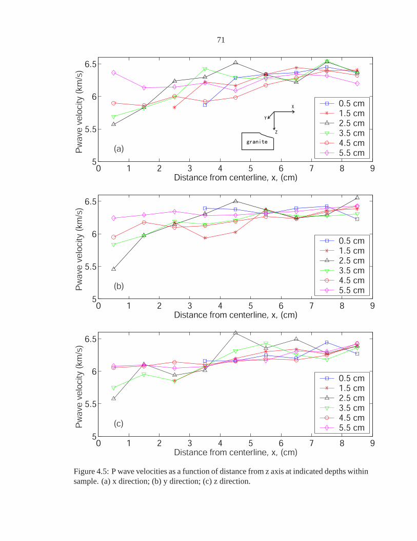
71

0 1 2 3 4 5 6 7 8 95

5.5

6

6.5

Distance from centerline, x, (cm)

Pw

ave

velo

city

(km

/s)

(a)

0.5 cm1.5 cm2.5 cm3.5 cm4.5 cm5.5 cm

0 1 2 3 4 5 6 7 8 95

5.5

6

6.5

Distance from centerline, x, (cm)

Pw

ave

velo

city

(km

/s)

(b)

0.5 cm1.5 cm2.5 cm3.5 cm4.5 cm5.5 cm

0 1 2 3 4 5 6 7 8 95

5.5

6

6.5

Distance from centerline, x, (cm)

Pw

ave

velo

city

(km

/s)

(c)

0.5 cm1.5 cm2.5 cm3.5 cm4.5 cm5.5 cm

Figure 4.5: P wave velocities as a function of distance from z axis at indicated depths withinsample. (a) x direction; (b) y direction; (c) z direction.

72

0 1 2 3 4 5 6 7 8 95

5.2

5.4

5.6

5.8

6

6.2

6.4

6.6

Distance from centerline (cm)

P−

wav

e ve

loci

ty (

km/s

)

4.5 cm depth

Vx

Vz

Figure 4.6: P wave velocities as a function of distance from z axis in x, y and z directionsat 4.5 cm depth below surface.

73

0 10 20 30 40 50

4.0

4.4

4.8

5.2

5.6

6.0

6.4

6.8

Vx

Vy

Vz

P-w

ave

velo

city

(km

/s)

Normalized distance, r/r0

Figure 4.7: Plot of all velocity measurements in three directions as function of distancefrom crater center. Curve line is exponential decay fit of data. See Equation 4.5.

74

tance from the impact point,r(r =

√x2 + z2

). The relation between the P wave velocity

and the radial distance, normalized by the radius of the projectile, 0.3 cm for this shot, is

found to follow an exponential decay relation:

Vp = 6.24(1− e(−0.26±0.01)r/r0

)(4.5)

The ultrasonic P wave velocity increase to its unshocked value atr/r0 equals 20, or, the

radial distance∼ 6 cm. This is in good agreement with the observation of the limit of radial

cracking that may be seen in the cross section after cutting the target open (Figure 3.17).

4.3.2 Attenuation measurements

Compressional wave attenuation coefficients are all calculated at frequency of 4.5 MHz, the

central peak of reflected wave from surface A (Figure 4.4) using Equations 4.3-4.4. The

accuracy of calculatingp using this pulse-echo method is estimated to be± 0.05 dB/cm

[Wepfer and Christensen, 1990]. Figure 4.8 shows the relation between the attenuation

coefficients versus the normalized radial distance from the impact point. The general trend

for the three directions is that the attenuation coefficients decrease with the increasing radial

distance from the impact point, following a power decay law:

αx = 15.17(r/r0)−0.17±0.03 (4.6a)

αy = 15.26(r/r0)−0.17±0.03 (4.6b)

αz = 12.02(r/r0)−0.14±0.03 (4.6c)

75

5 10 15 20 25 30 35 40 45 50

7

8

9

10

11

12

5 10 15 20 25 30 35 40 45 50

7

8

9

10

11

12

5 10 15 20 25 30 35 40 45 50

7

8

9

10

11

12

ap_x (

dB

/cm

)

Normalized distance, r/r0

ap_y (

dB

/cm

)

ap_z (

dB

/cm

)

Normalized distance, r/r

0

Normalized distance, r/r0

Figure 4.8: Attenuation coefficients as a function of normalized radial distance from impactpoint for three directions. Lines are power decay fit of data. (a) x; (b) y; (c) z.

76

The attenuation coefficients in x and y directions are similar but different from that in z

direction. It is obvious from Equations 4.6 and Figure 4.8 that at the same distance from

the impact point, attenuation parameters in z direction is smaller than those in x and y

directions. Therefore, the amplitude of compressional wave in z direction attenuates less

than those in the directions normal to the orientation of tensile cracks. This is because

tensile cracks extend mostly in z direction, and the effect of cracks on the amplitude of

ultrasonic wave is larger in directions normal to the orientation of cracks, which are x and

y directions, than that in the direction along crack orientation.

4.4 Analysis and discussion

For hypervelocity impact into brittle materials, both concentric/spherical and radial/tensile

cracks are produced (Figure 5 inPolanskey and Ahrens[1990]). The radial cracks propa-

gate further than the concentric cracks, since radial cracks are produced when the tensile

stress in the elastic regime is greater than the tensile strength of the material, which is usu-

ally smaller, by a factor of ten, than the compressive strength. Compressional wave velocity

is reduced substantially by cracks oriented with planes normal to the wave propagation di-

rection [Anderson et al., 1974;O’Connell and Budiansky, 1974]. In Figure 4.9, the plane

of cracks extends in the z direction. Velocity of compressional wave propagating in the x

direction is reduced more than that propagating in the z direction. Therefore, the reduction

of the measured compressional wave velocity in the x direction by the tensile cracks is ex-

pected to be higher than that in the other two directions, which agrees with our observed

results (Figure 4.5, 4.6). The fracture of a cracked media can be described by two rather

77

X

Z

Figure 4.9: Schematic diagram showing effect of aligned cracks on elastic waves propa-gating at different directions. Compressional wave velocity in x direction is reduced morethan that in z direction.

different but ultimately related parameters: (1) Damage parameter,D, used byGrady and

Kipp [1987] andAhrens and Rubin[1993]; is defined as:

D = 1−(

V

V0

)2

(4.7)

V andV0 are the effective and intrinsic velocity of the fractured body respectively. (2) Crack

density,ε (Equation 2.3).

The two parameters are closely related. In the work ofAshby and Sammis[1990] to

relate fracture to material strength reduction, damage in a body with inclined cracks of

length 2a is:

D =4

3π (αa)3 Nv (4.8)

whereα is a geometric constant, andNv is the number of cracks per unit volume. It is

78

obvious that this is the same concept as the crack density comparing equations 2.3 and 4.8.

In this study, definition of damage parameter in equation 4.7 is used, since it is directly

related to our velocity measurements.

From the measured compressional wave velocity of the samples,Dp is calculated from

Equation 4.7. Figure 4.10 shows the damage parameter versus the normalized radial dis-

tance from the impact point for the three orthogonal directions. The data are fitted by a

power decay law function:

Dx = 0.95 (r/r0)−0.53±0.08 (4.9a)

Dy = 0.99 (r/r0)−0.54±0.06 (4.9b)

Dz = 1.04 (r/r0)−0.5±0.08 (4.9c)

Although the measured data are quite scattered, the general trend is that the damage pa-

rameters in all the three directions decay with distance from the impact point. Anisotropy

is not very obvious from the damage parameter calculation.

The effective elastic moduli of a rockM (replaceM with the Young’s modulusE, bulk

modulusK, and shear modulusµ is a function of the intrinsic elastic moduli, the matrix and

fluid properties, the crack density (ε), the geometry of cracks and the interactions between

them [e.g.O’Connell and Budiansky, 1974].

The model ofO’Connell and Budiansky[1974] takes into account the interaction be-

tween cracks. It is well known that the solution based on this type of model often does not

correspond to experimental data for materials with big contrast in component properties

[Levin and Markvo, 2005]. According to their equations, the shear modulus becomes zero

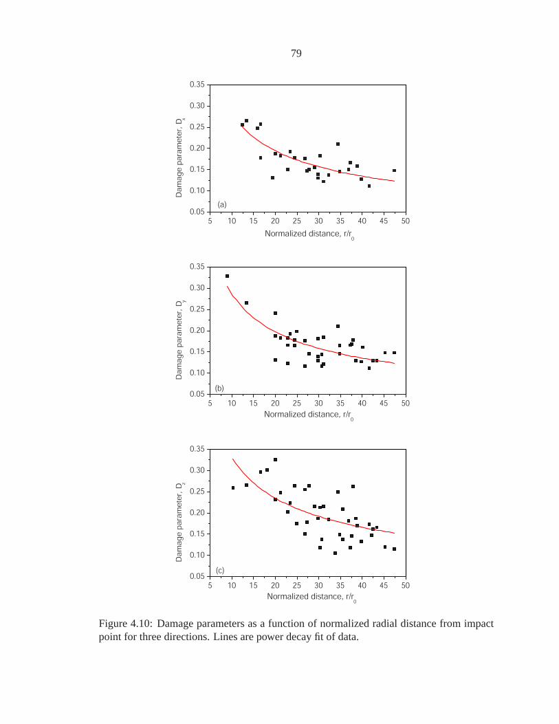
79

5 10 15 20 25 30 35 40 45 500.05

0.10

0.15

0.20

0.25

0.30

0.35

5 10 15 20 25 30 35 40 45 500.05

0.10

0.15

0.20

0.25

0.30

0.35

5 10 15 20 25 30 35 40 45 500.05

0.10

0.15

0.20

0.25

0.30

0.35

(a)

Damag

e pa

ram

ete

r, D

x

(b)

Da

mag

e pa

ram

ete

r, D

y

(c)

Da

ma

ge

pa

ram

ete

r, D

z

Normalized distance, r/r0

Normalized distance, r/r0

Normalized distance, r/r0

Figure 4.10: Damage parameters as a function of normalized radial distance from impactpoint for three directions. Lines are power decay fit of data.

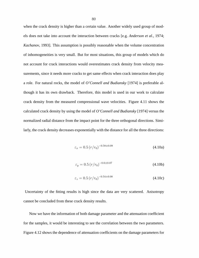
80

when the crack density is higher than a certain value. Another widely used group of mod-

els does not take into account the interaction between cracks [e.g.Anderson et al., 1974;

Kachanov, 1993]. This assumption is possibly reasonable when the volume concentration

of inhomogeneities is very small. But for most situations, this group of models which do

not account for crack interactions would overestimates crack density from velocity mea-

surements, since it needs more cracks to get same effects when crack interaction does play

a role. For natural rocks, the model ofO’Connell and Budiansky[1974] is preferable al-

though it has its own drawback. Therefore, this model is used in our work to calculate

crack density from the measured compressional wave velocities. Figure 4.11 shows the

calculated crack density by using the model ofO’Connell and Budiansky[1974] versus the

normalized radial distance from the impact point for the three orthogonal directions. Simi-

larly, the crack density decreases exponentially with the distance for all the three directions:

εx = 0.5 (r/r0)−0.58±0.09 (4.10a)

εy = 0.5 (r/r0)−0.6±0.07 (4.10b)

εz = 0.5 (r/r0)−0.54±0.08 (4.10c)

Uncertainty of the fitting results is high since the data are very scattered. Anisotropy

cannot be concluded from these crack density results.

Now we have the information of both damage parameter and the attenuation coefficient

for the samples, it would be interesting to see the correlation between the two parameters.

Figure 4.12 shows the dependence of attenuation coefficients on the damage parameters for

81

5 10 15 20 25 30 35 40 45 500.04

0.06

0.08

0.10

0.12

0.14

0.16

5 10 15 20 25 30 35 40 45 500.04

0.06

0.08

0.10

0.12

0.14

0.16

5 10 15 20 25 30 35 40 45 500.04

0.06

0.08

0.10

0.12

0.14

0.16

cra

ck d

en

sity

, X

crack

densi

ty, Y

crack

de

nsi

ty, Z

Normalized distance, r/r0

Normalized distance, r/r0

Normalized distance, r/r0

Figure 4.11: Crack densities inverted from measured P-wave velocity by using model ofO’Connell and Budiansky[1974] as function of normalized radial distance from impactpoint for three directions. Lines are power decay fit of data. (a) x; (b) y; (c) z.

82

0.05 0.10 0.15 0.20 0.25 0.30

7

8

9

10

11

0.05 0.10 0.15 0.20 0.25 0.30 0.35

7

8

9

10

11

0.10 0.15 0.20 0.25 0.30 0.35

7

8

9

10

11

ax(dB/cm)

Dx

ay(dB/cm)

Dy

az(dB/cm)

Dz

Figure 4.12: Attenuation coefficients versus damage parameter for three directions. (a) x;(b) y; (c) z. Lines are linear fit of data.

83

the cubes measured in the three directions. The attenuation coefficients increase with the

damage parameters consistently for the three situations. The data are fitted with:

αx = 5.94 + (16.59± 1.8) Dx (4.11a)

αy = 5.66 + (17.09± 1.6) Dy (4.11b)

αz = 5.97 + (7.79± 1.2) Dz (4.11c)

unit ofα is decibels per centimeter. The intercepts of these equations represent the intrinsic

values of the attenuation coefficients of the samples when there is no shock-induced damage

happened (D equals zero). The values for the three directions are very close (5.66 to 5.97).

However, the slope of the equation for z direction is only about half of the values of x and

y directions. This means that for the same damage parameter obtained from measured P

wave velocity, the attenuation coefficient in z direction is smaller than the values in x and

y directions. The tensile cracks propagating in the impact direction has a larger effect on

the attenuation coefficients in directions perpendicular with it. Therefore, the attenuation

coefficient is a more useful parameter than the wave velocity in describing the anisotropic

orientation of cracks.

Combined with velocity measurement, attenuation coefficient,αp, can provide mi-

crostructure information of cracked media.Liu and Ahrens[1997] gave an empirical re-

lation of crack length (a), crack density (ε) and attenuation coefficient for San Marcos

gabbro:

a =hε

αp

(4.12)

84

whereh is an undetermined material constant. More work should be carried out in the

future to get further information about the microstructure of the media studied.

4.5 Concluding remarks

1 cm cubes are cut from a San Marcos granite target block recovered from an impact cra-

tering experiment. Both compressional wave velocity and attenuation measurements are

conducted on these cubes in three orthogonal directions. Damage parameter is calculated

from the measured P wave velocity. The theory ofO’Connell and Budiansky[1974] is used

to calculate the crack density of the cracked media from the measured velocity. The main

conclusions obtained from this study are listed as follows:

1. Anisotropy is observed from the ultrasonic velocity and attenuation measurement,

but not very obvious from the calculated damage parameter and crack density.

2. The measured P wave velocity and the normalized radial distance from the impact

point follow an exponential decay relation, shown in equation 4.5.

3. The change of rock properties (D, ε, α) beyond shock pressure regime 1 with the

normalized radial distance from the impact point can be expressed by:

(D, ε, α) = α (r/r0)b (4.13)

wherea andb are fitted constants.

4. Attenuation coefficient is a more useful parameter than elastic velocity in studying

85

the anisotropic orientation of cracks. From Equation 4.11, slope of the linear relation

of attenuation coefficient versus damage parameter in x and y directions is about

twice of the value in z direction.

.

Acknowledgments: We appreciate the technical support of E. Gelle, M. Long. We

thank Professor G. Ravichandran for the use of ultrasonic attenuation apparatus. We also

thank Shiming Zhuang, Tracy Kidd, and Daoyuan Sun for their thoughtful suggestions and

discussion.

86

Chapter 5

Scaling Law

5.1 Introduction

The formation of an impact crater is a combined effect of the size and material of impactor,

the impact velocity, the target material property, and other variables such as local grav-

ity. Cm scale experimental study as well as large scale numerical simulations have been

carried out over several decades to study the dependence of impact consequence, such as

crater ejecta and crater morphology, on the impact conditions [e.g.Holsapple and Schmidt,

1982;Housen et al., 1983;Kadono and Fujiwara, 2005;O’Keefe and Ahrens, 1981]. The

outcome of one impact event can be predicted from the result of others based on the scaled

relations.

The simplest and most common variables used for scaling are size and velocity pa-

rameters, but other variables such as gravitational field or material strength can also be

included. Holsapple[1993] combined a detailed dimensional analysis of scaling for im-

pact processes. For example, the crater dimension such as volume and depth resulted from

a hypervelocity impact can be expressed as function of impactor size and velocity, target

strength, and gravity [Holsapple, 1993]. Various scaling rules exist in the literature for

87

crater volume and depth, since these variables are easiest to measure for a hypervelocity

impact and thus most commonly used in the impact cratering community.

Shock-induced damage and cracking beneath impact craters are less affected by the

late stage modification to craters and therefore possible indicator of impact conditions. The

damage and cracking have long been recognized on Earth and the Moon [e.g.Ackermann

et al., 1975;Simmons et al., 1973]. Preliminary work has been carried out to study damage

and cracking beneath craters in the laboratory recently [e.g.Ahrens and Rubin, 1993;Xia

and Ahrens, 2001]. It has been suggested that the cracking information for impact crater is

a very useful constraint for the impact history [Ai and Ahrens, 2004].

Surprisedly, damage and cracking beneath an impact crater has not yet been studied

systematically. The purpose of this work is to explore this important yet not well under-

stood aspect of craters experimentally and to construct a scaling law for damage depth.

Section 5.2 gives the theoretical dimensional analysis. The experimental data are presented

and discussed in section 5.3. Section 5.4 is the summary and future work.

5.2 Dimensional analysis

Dimensional analysis for impact cratering is traditionally conducted in ”strength” and

”gravity regime” [Holsapple, 1993]. Surprisingly, no clear definition of strength has been

given in the available references. It is appropriate to start our dimensional discussion with

clarifying some relevant terminologies. According toSingh[1989], strength of rock is the

ability to resist loads without yielding or fracturing. Ultimate strength of a rock is the max-

imum value of stress attained before fracture. Tensile strength is the ultimate strength in

88

tension, while compressive strength is the ultimate strength in compression. The ”strength”

term, Y, to be used in the next part, refers to the uniaxial compressive strength, which is

obtained through uniaxial stress loading test.

Consider the most common and simplest situation: a target material with mass density

ρt and compressive strengthY impacted by a projectile with radiusa and mass densityρp at

impact velocityV. The surface gravity isg. A single measure of the crater (C), is a function

of these variables:

C = f(a, ρp, V ; ρt, Y ; g) (5.1)

Left side of the equation can be replaced by crater volume, crater depth and radius, ejecta,

etc. According to the dimensional analysis ofHolsapple[1993], Equation 5.1 can be sim-

plified using four dimensionless combinations:

C = f(ga

U2,

Y

ρtU2,ρt

ρp

) (5.2)

C is normalized measure of the crater. For example,ρtV/m for crater volume,h/a for

crater depth, etc. The first term on the right side, traditionally referred asπ2, represents

the effect of gravity level on the crater. The second term represents the effect of material

strength, and is denoted asπ3. The third term is the ratio of mass densities of target and

projectile. When the projectile is kilometer-sized, the effect of gravity is large compared

with the strength of target, the strength term is ignored (”gravity regime”). Equation 5.2 is

simplified into:

C = f(ga

U2,ρt

ρp

) (5.3)

89

On the other hand, when the projectile is only centimeter or meter-sized, the strength of

target is more important (”strength regime”). Equation 5.2 becomes:

C = f(Y

ρtU2,ρt

ρp

) (5.4)

For our experiments carried out at cm scale, strength of the target material is large compared

to the lithostatic pressure. Therefore,π2 is ignored in this work, and Equation 5.4 is used

for the next discussion.

Historical scaling approaches to impact cratering showed that the relation between the

crater dimension and the strength or gravity term follows a power law [e.g.Holsapple,

1993;Schmidt and Housen, 1987]. The density ratio also has effect on the crater morphol-

ogy. It has been reported that the crater depth is proportional toρp/ρt [e.g. Love et al.,

1993]. InSchmidt and Housen[1987], the normalized crater volume in the strength regime

is expressed as:

ρtV

m=

(ρt

ρp

)1−3v (Y

ρtU2

)−3µ2

(5.5)

whereµ andv are scaling exponents to be determined. Again, the left side of Equation 5.5

can be replaced by other measurements of the impact crater, such as crater depth, ejecta

velocity, etc.

Damage and fracture feature of impact craters are studied in this work. Here the damage

depthDd is defined as the deepest distance cracks propagate beneath the impact crater, as

shown in Figure 3.17). If damage depth of impact crater also follows a power law relation

with the strength scaled size (π3), like other crater measurements such as volume, then the

90

damage information could be a very useful constraint for impact history. And this is the

focus of the next section.

5.3 Experimental data and discussion

Two types of rocks, San Marcos granite and Bedford limestone, are chosen since they are

representative of crustal rocks. The compressive strength of the two types of rocks are

∼ 300 MPa and∼ 120 MPa respectively. These values are taken fromSingh[1989], of

which the strength of granite is the average value of the data available for granites in their

work. Impacts at different combinations of projectile material, size and impact velocity are

carried out. Table 5.1 summarizes the impact conditions and the damage depth as well as

the final crater dimensions including crater volume, diameter and crater depth for a series

of experiments carried out in this study. Shots of 8409001 to 0909 are taken fromPolanskey

and Ahrens[1990], but the damage depths for these recovered targets are measured in this

study. The impact velocities vary from as low as 0.276 km/s to 6.49 km/s. The diameter

of projectile starts from 0.318 cm for the higher velocity impacts, to 1.27 cm for the lower

velocity impacts.

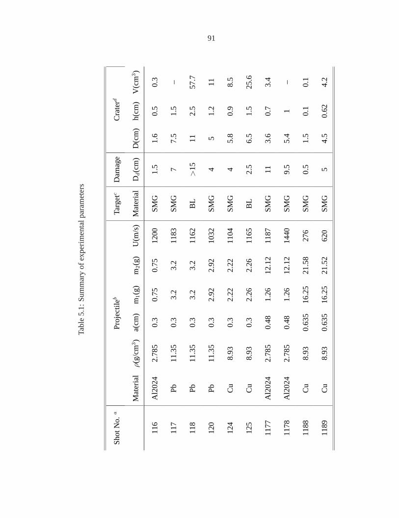
91

Tabl

e5.

1:S

umm

ary

ofex

perim

enta

lpar

amet

ers

Sho

tNo.

aP

roje

ctile

bTa

rgetc

Dam

age

Cra

terd

Mat

eria

lρ(g

/cm

3)

a(cm

)m 1

(g)

m2(g

)U

(m/s

)M

ater

ial

Dd(c

m)

D(c

m)

h(cm

)V

(cm3

)

116

Al2

024

2.78

50.

30.

750.

7512

00S

MG

1.5

1.6

0.5

0.3

117

Pb

11.3

50.

33.

23.

211

83S

MG

77.

51.

5–

118

Pb

11.3

50.

33.

23.

211

62B

L>

1511

2.5

57.7

120

Pb

11.3

50.

32.

922.

9210

32S

MG

45

1.2

11

124

Cu

8.93

0.3

2.22

2.22

1104

SM

G4

5.8

0.9

8.5

125

Cu

8.93

0.3

2.26

2.26

1165

BL

2.5

6.5

1.5

25.6

1177

Al2

024

2.78

50.

481.

2612

.12

1187

SM

G11

3.6

0.7

3.4

1178

Al2

024

2.78

50.

481.

2612

.12

1440

SM

G9.

55.

41

–

1188

Cu

8.93

0.63

516

.25

21.5

827

6S

MG

0.5

1.5

0.1

0.1

1189

Cu

8.93

0.63

516

.25

21.5

262

0S

MG

54.

50.

624.

2

92

Tabl

e5.

1:(c

ontin

ued)

Sho

tNo.

aP

roje

ctile

bTa

rgetc

Dam

age

Cra

terd

Mat

eria

lρ(g

/cm

3)

a(cm

)m 1

(g)

m2(g

)U

(m/s

)M

ater

ial

Dd(c

m)

D(c

m)

h(cm

)V

(cm3

)

1191

Al2

024

2.78

50.

635

6.61

10.3

113

95S

MG

129.

21.

322

.5

1194

Cu

8.93

0.63

516

.45

21.7

169

0S

MG

95.

50.

87.

3

1195

Cu

8.93

0.48

8.35

14.3

195

8S

MG

127.

21.

216

.7

1196

Al2

024

2.78

50.

635

6.64

10.3

472

0S

MG

13

0.3

1.0

1197

Cu

8.93

0.63

516

.35

21.7

540

BL

149

1.3

41.8

1199

Cu

8.93

0.48

8.35

14.2

960

0B

L6.

58.

51.

526

.8

1200

Al2

024

2.78

50.

482.

68.

5399

0S

MG

13.

50.

52.

2

1201

Al2

024

2.78

50.

635

5.02

10.2

966

0B

L6

5.1

112

.8

1202

Al2

024

2.78

50.

482.

598.

5398

6B

L13

7.4

1.2

36.5

1203

Cu

8.93

0.48

8.35

14.2

875

0S

MG

>10

--

-

1204

Cu

8.93

0.48

8.36

14.2

756

0S

MG

32.

70.

41.

1

93

Tabl

e5.

1:(c

ontin

ued)

Sho

tNo.

aP

roje

ctile

bTa

rgetc

Dam

age

Cra

terd

Mat

eria

lρ(g

/cm

3)

a(cm

)m 1

(g)

m2(g

)U

(m/s

)M

ater

ial

Dd(c

m)

D(c

m)

h(cm

)V

(cm3

)

1205

Pb

11.3

50.

4810

.15

16.0

610

90S

MG

>15

--

-

1206

Pb

11.3

50.

4810

.216

.13

600

SM

G1

3.5

0.5

1.9

1207

Pb

11.3

50.

635

19.6

524

.91

590

SM

G5.

54

0.6

3.8

1208

Pb

11.3

50.

635

19.6

524

.980

0S

MG

127

1.1

28.3

1209

Pb

11.3

50.

4810

.216

.12

590

BL

138

1.5

36.7

8409

01A

l2.

785

0.15

90.

0443

0.04

4364

90S

MG

a2

6.5

19

8409

02F

e7.

740.

159

0.12

920.

1292

4600

SM

Ga

49.

81.

530

8409

04F

e7.

740.

159

0.12

970.

1297

5440

SM

Ga

4.5

10.5

1.65

36

8409

05F

e7.

740.

159

0.12

970.

1297

4600

SM

Ga

3.2

81.

4519

8409

06F

e7.

740.

159

0.12

970.

1297

4760

SM

Ga

3.5

9.2

1.4

23

8409

07ba

salt

2.75

0.23

80.

1557

0.15

5722

60S

MG

a1.

53.

50.

72.

3

94

Tabl

e5.

1:(c

ontin

ued)

Sho

tNo.

aP

roje

ctile

bTa

rgetc

Dam

age

Cra

terd

Mat

eria

lρ(g

/cm

3)

a(cm

)m 1

(g)

m2(g

)U

(m/s

)M

ater

ial

Dd(c

m)

D(c

m)

h(cm

)V

(cm3

)

8409

09st

eel

7.85

0.31

81.

0571

1.05

7116

90S

MG

a5

8.3

1.4

25.5

a11

6-12

5:T

his

stud

y,rifl

esh

ot;1

177-

1209

:T

his

stud

y,20

mm

prop

ella

ntgu

n;84

0901

-090

9:P

ola

nsk

eya

nd

Ah

ren

s[199

0]

bm

1:

mas

sof

proj

ectil

eon

ly;m

2:

mas

sof

proj

ectil

ean

dsa

bot.

cS

MG

:San

Mar

cos

gran

ite;B

L:B

edfo

rdlim

esto

ne;S

MG

a:S

anM

arco

sga

bbro

.

dD

:dia

met

er;h

:cr

ater

dept

h;V

:cra

ter

volu

me.

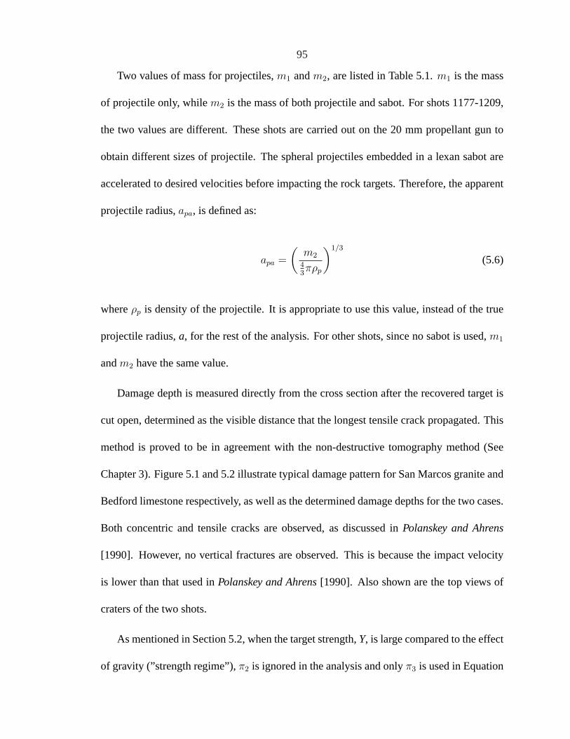
95

Two values of mass for projectiles,m1 andm2, are listed in Table 5.1.m1 is the mass

of projectile only, whilem2 is the mass of both projectile and sabot. For shots 1177-1209,

the two values are different. These shots are carried out on the 20 mm propellant gun to

obtain different sizes of projectile. The spheral projectiles embedded in a lexan sabot are

accelerated to desired velocities before impacting the rock targets. Therefore, the apparent

projectile radius,apa, is defined as:

apa =

(m2

43πρp

)1/3

(5.6)

whereρp is density of the projectile. It is appropriate to use this value, instead of the true

projectile radius,a, for the rest of the analysis. For other shots, since no sabot is used,m1

andm2 have the same value.

Damage depth is measured directly from the cross section after the recovered target is

cut open, determined as the visible distance that the longest tensile crack propagated. This

method is proved to be in agreement with the non-destructive tomography method (See

Chapter 3). Figure 5.1 and 5.2 illustrate typical damage pattern for San Marcos granite and

Bedford limestone respectively, as well as the determined damage depths for the two cases.

Both concentric and tensile cracks are observed, as discussed inPolanskey and Ahrens

[1990]. However, no vertical fractures are observed. This is because the impact velocity

is lower than that used inPolanskey and Ahrens[1990]. Also shown are the top views of

craters of the two shots.

As mentioned in Section 5.2, when the target strength,Y, is large compared to the effect

of gravity (”strength regime”),π2 is ignored in the analysis and onlyπ3 is used in Equation

96

Crater

Position for (b)

(a)

~ 1

2 c

m

(b)

Figure 5.1: Shot 1208, granite impacted by∼25 g lead ball (with sabot) at 800 m/s. Scaleis 5 cm. (a) Top view showing impact crater. Also shown is cross section position for (b);(b) Cross section of target after being cut open. Tensile cracks extend to∼12 cm for thiscase.

97

Crater

Position of (b)

(a)

~ 1

3 c

m

(b)

Figure 5.2: Shot 1209, limestone impacted by∼16 g (with sabot) lead ball at 590 m/s.Scale is 5 cm. (a) Top view; (b) Cross section showing tensile cracks extend to∼ 13 cmfor this case.

98

5.2. This is true for our experiments carried out at cm scale. The effect of gravity, termπ2

is ignored throughout the analysis in this work.

Based on the dimensional analysis in the previous section, the damage depth of craters

listed in Table 5.1 normalized by the apparent projectile radius,apa, over the projectile-to-

target density ratio, is plotted versus the strength parameter,π3, as shown in Figure 5.3.

The strength size extends from10−3 to 101, and the normalized damage depth over density

ratio extends from100 to 104. As expected, the damage depth generally follow a power-

law trend. The slope of the fitted line is -1.27, which corresponds to the value ofµ as 0.8,

according to Equation 5.5. For comparison, both energy and momentum scaling are also

plotted in the figure. Slope of energy scaling is -1, corresponding toµ=2/3, while slope of

momentum is -0.5, corresponding toµ=1/3. Fitting result of our data follows the energy

scaling. This result is very interesting and intriguing, since this indicates that the damage

beneath craters is a function of of impact conditions and the damage information could be

used as a very useful constraint for impact history. However, no damage depth data of cm

scale experiments are available from literature.

The normalized crater volume over density ratio is also plotted versus the strength pa-

rameter,π3 (Figure 5.4). The normalized crater volume extends from10−3 to 103. Also

included are data fromPayne[1965] for impacts into metals. It is observed that the data

from this study and those fromPolanskey and Ahrens[1990] follow the same trend, but

not the data fromPayne[1965] for metals. Data from this study and those fromPolanskey

and Ahrens[1990] are fitted by a power-law function. The slope of the fitted line is -1.79,

which implies thatµ=1.2 according to Equation 5.5. This inconsistency might be caused

99

10-3

10 -2

10 -1

100

101

100

101

102

103

104

slope= -1.27( = 0.8)Energy scaling

slope= 1( =2/3)

Momentum scalingslope= 0.5( =1/3)

3,Y/

t U2

(Dd/a

pa)/(

p/

t)

SMG, this studyBL, this studyPolanskey & Ahrens (1990)fitted

π

ρ

ρ

ρ

µ

µµ -

-

Figure 5.3: Normalized crater damage depth by apparent projectile radius,Dd/apa, overprojectile-density ratio,ρp/ρt, as power-law function of strength parameter,π3 = Y/ρtU

2.Slope of fitted line is -1.27. Note log-log scale of the plot.

100

10-5

10 -4

10 -3

10 -2

10 -1

100

101

10 -3

10 -2

10 -1

100

101

102

103

104

slope=

1.79( =1.2)

Energy scalingslope= 1( =2/3)

Momentum scalingslope= 0.5( =1/3)

3,Y/

t U2

V,

t V/m

/(p/

t)

SMG, this studyBL, this studyPolanskey & Ahrens (1990)Payne (1965), metalfitted

π

π

ρ

ρρ

ρ

µ

µ

µ

-

-

-

-

Figure 5.4: Normalized crater volume by apparent projectile volume,ρtV/m as a functionof strength parameter,π3. Definition of parameters are same as in Figure 5.3. Data forimpacts into metal taken fromPayne[1965] are also plotted for comparison. Slope of fittedline is -1.79.

101

0 5 10 15 20 250

0.5

1

1.5

2

2.5

3

3.5

Crater diameter, cm

Cra

ter

dep

th,

cm

slope=0.12

SMG, this studyBL, this studyPolanskey & Ahrens (1990)Schmidt 87, sandfitted

Figure 5.5: Plot of crater depth as a function of crater diameter. Linear relation is observed,and slope is 0.12.

102

by confusion of definition of ”strength” in literature. Strength is a strain rate dependent

material constant, as discussed in Chapter 2. Strength for materials under hypervelocity

impact is higher than that of relatively lower velocity impact. Again, both energy and mo-

mentum scaling are shown in this figure for comparison. Our result shows the combining

effect of strain rate on strength and energy scaling.

The crater depth as a function of crater diameter is plotted in Figure 5.5. For compar-

ison, data fromSchmidt and Housen[1987] are included. A very clear linear relation is

observed for all the data, and the slope is 0.12.

5.4 Summary

Two types of rocks, San Marcos granite and Bedford limestone, were impacted by pro-

jectiles with various sizes and types at different velocities. Damage depth,Dd for these

hypervelocity impact craters was discussed in this work. It was found that the damage

depth is a function of the impact velocity and the physical properties of target/projectile

combination. In general, the damage depth normalized by the apparent projectile radius,

apa, follows a power-law function with the strength scaled size, which can be expressed as:

Dd

apa

∝(

ρp

ρt

)A (Y

ρtU2

)B

(5.7)

whereA andB are constants. In this study,A equals 1 andB equals -1.27. This indicates

that the damage depth would be an important measure for impact craters, yet not being

studied systematically before. If combined with other measures such as crater volume and

103

depth, it is possible that the damage depth can provide useful constrains for impact history.

This work is the preliminary step in studying damage depth for impact craters. There

are still a lot of issues to be explored. Data on damage information of impact craters, both

from laboratory experiments and from craters in the field, are relatively scarce. More lab-

oratory data are needed under controlled conditions. First, more types of targets such as

sand, sandstone, ice, etc, should be tested to represent the terrestrial and extraterrestrial

surfaces. Second, impact at different angles should be carried out systematically. Third,

effect of gravity is ignored in this work. However, this important effect should be included

in the future. Experiments at different gravity scale should be carried out. Fourth, numer-

ical calculation of large scale impacts should be used as a complimentary tool to simulate

impacts at different impact conditions, including the effect of gravity.

Although our work is only the first step in exploring the damage beneath impact crater,

the result is very intriguing. Information of shock-induced damage and cracking below

impact craters is an important constraint for impact history. It sheds light on the possibility

of using damage information of craters as a constraint for impact history. Combined with

other known parameters such as crater dimension, projectile and target properties, damage

and cracking could provide useful yet unrecognized information on the impact history.

Our work will provide a direction for deploying seismic investigation of low-velocity zone

beneath impact craters in the field.

104

Chapter 6

Shock-Induced Damage beneathOblique Impact Craters

6.1 Introduction

Natural impact events always happen at impact angles less than vertical [Gilbert, 1893;

Shoemaker, 1962]. However, a large amount of work in the impact cratering field, both

theoretical and experimental, is performed under normal impact condition to allow the

simplification of the problem to two dimensions because of axial symmetry, since vertical

impacts are regarded as a good representation of oblique impacts based on the fact that

oblique hypervelocity impacts with impact angle higher than 30o (90o means vertical im-

pact) produce circular craters similar to that observed in vertical hypervelocity impacts,

according to the comprehensive study ofGault [1978].

Oblique impact craters, Chicxulub and Mansion for example [Schultz and Anderson,

1996;Schultz and D’Hondt, 1996], are often identified by the ejecta pattern, the geophysi-

cal features of the crater, and/or the elongated crater shape for craters impacted at extremely

low angles. However, late stage collapse of the crater and geological process such as ero-

sion and sedimentation would modify and mask some of these features.

105

The increase of computation capability of computers during the last decade makes it

possible to carry out three dimensional numerical simulations of hypervelocity oblique

impacts. Pierazzo and Melosh[2000] did calculation for hypervelocity oblique impacts

at different impact angles and concluded that even though the position of the shock front

as it propagates through the target appears symmetric around the impact point for oblique

impacts, the peak shock pressure experienced by the rock target is asymmetric (Figure 6.1).

Dahl and Schultz[2001] also observed stress wave asymmetries in oblique hypervelocity

impact experiments. Unfortunately, stress wave cannot be measured directly for a natural

impact crater in the field. But this intriguing result leads us to look into the shock-induced

damage and cracking, which is directly related to the peak shock pressure, beneath craters

by oblique impacts.

From the discussion of previous chapters, shock-induced damage beneath impact crater

is a potential constraint for impact history. However, the shock-induced damage beneath

oblique impact craters has not been paid attention to by far. This study presents results of

laboratory oblique impacts designed to measure the shock-induced damage beneath impact

craters. Again, San Marcos granite and Bedford limestone, are chosen as target materials

[e.g.Ai and Ahrens, 2004;Ahrens and Rubin, 1993], because they provide convenient rep-

resentative material for low-porosity crystalline rock and high-porosity sedimentary rock.

The low velocity zone beneath the craters caused by shock-induced damage in the recov-

ered targets is mapped.

106

Fig

ure

6.1:

Pea

ksh

ock

pres

sure

cont

ours

inth

epl

ane

ofim

pact

for

ase

ries

of3D

hydr

ocod

esi

mul

atio

nsat

vario

usim

pact

angl

es.

The

proj

ectil

e,10

kmin

diam

eter

,is

show

nfo

rsc

ale.Ve

cto

rsill

ustr

ate

the

dire

ctio

nof

impa

ct.

Fro

mPie

razz

oa

nd

Me

losh[

2000

],F

igur

e3.

107

6.2 Experiments

Initially, 20x20x15 cm blocks were cut from San Marcos granite and Bedford limestone.

Cratering experimental setup is the same as that described in Chapter 3, except that the

impact angle is at 45o. The projectile used for both shots is a lead bullet, with radius of

0.3 cm and mass of 3.2 g. Impact velocity into granite is 1.2 km/s, and 1.16 km/s for

limestone. The impact velocity is chosen not to fragment the target, while to still produce

measurable compressional wave velocity reduction caused by the shock-induced damage

in the recovered target.

The compressional wave velocities beneath the oblique impact craters are mapped on

two central planes, one is plane A, the plane containing the projectile trajectory; the other

is plane B, the plane normal to plane A (Figure 6.2a). The tomography method described

in Chapter 3 is used for mapping the velocity structure in San Marcos granite. For Bedford

limestone, dicing method described in Chapter 4 is used to measure the velocity directly.

6.3 Results and discussion

6.3.1 Experimental results

Figure 6.3 shows the inverted compressional wave velocity structures of Plane A and B to

depth of 4 cm, for the recovered San Marcos granite block. The lowest P-wave velocity in

the highly damaged region beneath and near the crater reaches∼ 5 km/s (Figure 6.3), and

the reduction is∼ 20% from the intrinsic velocity of 6.3± 0.1 km/s, determined at 5 MHz.

The depth of the low velocity zones for this recovered granite target extends to 2-3 cm on

108

Plane A

Containing trajectory

Plane B

Normal to Plane A

Projectile

20 cm

20 cm

15 c

m

(a)

20 cm

20 c

m

1 cm

20 cm

15 c

m

1 cm

1 cm

X

Z

Α Β

(b)

Figure 6.2: (a) Oblique impact geometry of 20x20x15 cm block. Tomography measure-ment carried out on two central planes. Plane A containing projectile trajectory, plane Bis normal to plane A; (b) Diagram showing orientation for dicing method for limestone. 1cm center plane cut from the recovered target, then 1-cm cube cut from the center plane forvelocity measurement in two orthogonal directions, X and Z, which are the horizontal andvertical impact direction respectively.

109

both profiles for Plane A and B. Asymmetry is observed, although not very obvious, for

the inverted compressional wave structure of Plane A, the plane containing the projectile

trajectory (Figure 6.3a). Peak damage extends along the downrange direction from the

impact point. Asymmetry is not observed for Plane B, the plane normal to Plane A (Figure

6.3b).

In the field, craters larger than 1 km in diameter would inevitably experience uplift as

well as late stage modification such as erosion [Melosh, 1989]. Although the morphology or

the crater could be modified by such processes greatly, geophysical features such as gravity

anomaly and low seismic velocity structure beneath impact craters would be preserved

and are possible to be used as constraints for impact history. To simulate the erosion of

upper surface of the crater, a top layer of one centimeter thickness is cut off and the P-

wave velocity profiles of the two center planes of the remaining granite block are mapped

again using the tomography method. The inverted results for the two planes from the

top surfaces to 3 cm depth (the same position of 4 cm depth as before cut) are shown in

Figure 6.4. Similarly, asymmetry of the low velocity zone is observed in Plane A, the plane

containing the projectile trajectory, and higher reduction of the velocity is observed along

the downrange (Figure 6.4a). The damage pattern in Plane B, the plane normal to Plane B

is relatively symmetric (Figure 6.4b).

Compressional velocity measurements of Plane A and Plane B for the recovered Bed-

ford limestone using the dicing method are listed in Table 6.1 and 6.2 and shown in Figure

6.5 and 6.6. The measurement is carried out in two orthogonal directions, x, defined as the

horizontal direction which is parallel to the impact surface, and z, which is perpendicular

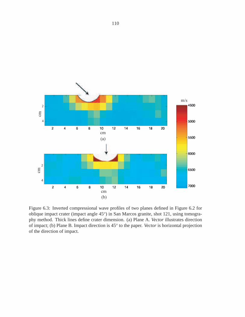
110

cm

cm

(a)

m/s

2

4

cm

cm

(b)

2

4

Figure 6.3: Inverted compressional wave profiles of two planes defined in Figure 6.2 foroblique impact crater (impact angle 45o) in San Marcos granite, shot 121, using tomogra-phy method. Thick lines define crater dimension. (a) Plane A.Vectorillustrates directionof impact; (b) Plane B. Impact direction is 45o to the paper.Vectoris horizontal projectionof the direction of impact.

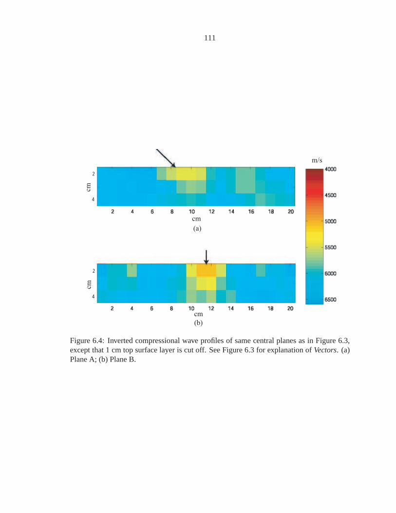
111

cm

cm

(a)

m/s

cm

cm

(b)

2

4

2

4

Figure 6.4: Inverted compressional wave profiles of same central planes as in Figure 6.3,except that 1 cm top surface layer is cut off. See Figure 6.3 for explanation ofVectors. (a)Plane A; (b) Plane B.

112

with the impact surface (See Figure 6.2b for detailed explanation of the orientation). For

those cubes beneath and near the impact crater region, the low velocity can be as low as

2.7 km/s, with the reduction of∼ 40%, from 4.6± 0.2 km/s, the intrinsic compressional

velocity of Bedford limestone [Ahrens and Rubin, 1993]. The damage depth identified

from these inverted results extends to 3∼4 cm for this oblique impact shot into Bedford

limestone. Both directions, x and z, of Plane A, the plane containing the projectile trajec-

tory, show asymmetric pattern; and higher velocity reduction is observed in the downrange

(Figure 6.5). In contrast, the inverted result for Plane B, which is the plane normal to Plane

A, shows a more symmetric pattern (Figure 6.6).

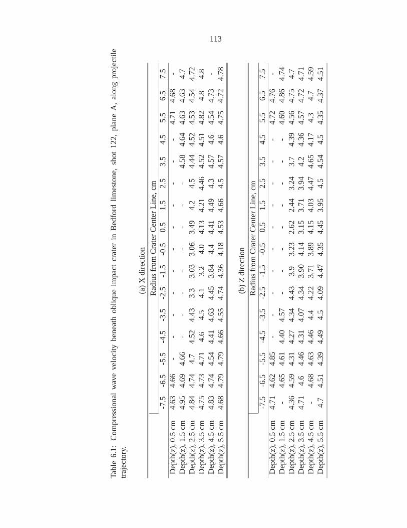
113

Tabl

e6.

1:C

ompr

essi

onal

wav

eve

loci

tybe

neat

hob

lique

impa

ctcr

ater

inB

edfo

rdlim

esto

ne,

shot

122,

plan

eA

,al

ong

proj

ectil

etr

ajec

tory

.

(a)

Xdi

rect

ion

Rad

ius

from

Cra

ter

Cen

ter

Line

,cm

-7.5

-6.5

-5.5

-4.5

-3.5

-2.5

-1.5

-0.5

0.5

1.5

2.5

3.5

4.5

5.5

6.5

7.5

Dep

th(z

),0.

5cm

4.63

4.66

--

--

--

--

--

-4.

714.

68-

Dep

th(z

),1.

5cm

4.95

4.69

4.66

--

--

--

--

4.58

4.64

4.63

4.63

4.7

Dep

th(z

),2.

5cm

4.84

4.74

4.7

4.52

4.43

3.3

3.03

3.06

3.49

4.2

4.5

4.44

4.52

4.53

4.54

4.72

Dep

th(z

),3.

5cm

4.75

4.73

4.71

4.6

4.5

4.1

3.2

4.0

4.13

4.21

4.46

4.52

4.51

4.82

4.8

4.8

Dep

th(z

),4.

5cm

4.83

4.74

4.54

4.41

4.63

4.45

3.84

4.4

4.41

4.49

4.3

4.57

4.6

4.54

4.73

-D

epth

(z),

5.5

cm4.

684.

794.

794.

664.

554.

744.

364.

184.

534.

664.

54.

574.

64.

754.

724.

78

(b)

Zdi

rect

ion

Rad

ius

from

Cra

ter

Cen

ter

Line

,cm

-7.5

-6.5

-5.5

-4.5

-3.5

-2.5

-1.5

-0.5

0.5

1.5

2.5

3.5

4.5

5.5

6.5

7.5

Dep

th(z

),0.

5cm

4.71

4.62

4.85

--

--

--

--

--

4.72

4.76

-D

epth

(z),

1.5

cm-

4.65

4.61

4.40

4.57

--

--

--

--

4.60

4.86

4.74

Dep

th(z

),2.

5cm

4.36

4.59

4.31

4.27

4.34

4.43

3.9

3.23

2.62

2.44

3.24

3.7

4.39

4.56

4.75

4.7

Dep

th(z

),3.

5cm

4.71

4.6

4.46

4.31

4.07

4.34

3.90

4.14

3.15

3.71

3.94

4.2

4.36

4.57

4.72

4.71

Dep

th(z

),4.

5cm

-4.

684.

634.

464.

44.

223.

713.

894.

154.

034.

474.

654.

174.

34.

74.

59D

epth

(z),

5.5

cm4.

74.

514.

394.

494.

54.

094.

474.

354.

453.

954.

54.

544.

54.

354.

374.

51

114

Tabl

e6.

2:C

ompr

essi

onal

wav

eve

loci

tybe

neat

hob

lique

impa

ctcr

ater

inB

edfo

rdlim

esto

ne,

shot

122,

plan

eB

,N

orm

alto

proj

ectil

etr

ajec

tory

.

(a)

Xdi

rect

ion

Rad

ius

from

Cra

ter

Cen

ter

Line

,cm

-6.5

-5.5

-4.5

-3.5

-2.5

-1.5

-0.5

0.5

1.5

2.5

3.5

4.5

5.5

6.5

Dep

th(z

),0.

5cm

--

--

--

--

--

-4.

714.

744.

87D

epth

(z),

1.5

cm5.

064.

894.

78-

--

--

-4.

264.

354.

444.

914.

74D

epth

(z),

2.5

cm5.

094.

854.

844.

664.

243.

463.

34.

434.

254.

544.

594.

764.

684.

86D

epth

(z),

3.5

cm4.

794.

744.

724.

74.

674.

274.

14.

34.

584.

474.

714.

754.

834.

65D

epth

(z),

4.5

cm4.

774.

514.

554.

754.

794.

64.

454.

634.

594.

434.

564.

424.

424.

75D

epth

(z),

5.5

cm4.

724.

554.

494.

654.

724.

654.

744.

554.

734.

734.

584.

574.

674.

61

(b)

Zdi

rect

ion

Rad

ius

from

Cra

ter

Cen

ter

Line

,cm

-6.5

-5.5

-4.5

-3.5

-2.5

-1.5

-0.5

0.5

1.5

2.5

3.5

4.5

5.5

6.5

Dep

th(z

),0.

5cm

--

--

--

--

--

-4.

64.

724.

78D

epth

(z),

1.5

cm4.

914.

874.

7-

--

--

--

4.52

4.66

4.65

5.02

Dep

th(z

),2.

5cm

5.02

4.9

4.7

4.4

4.03

3.22

3.24

3.7

4.03

4.42

4.66

4.78

4.69

5.0

Dep

th(z

),3.

5cm

4.93

4.86

4.8

4.82

4.64

3.84

3.94

4.5

4.53

4.4

4.57

4.79

4.74

4.89

Dep

th(z

),4.

5cm

4.76

4.83

4.29

4.6

4.89

4.49

4.47

4.65

4.47

4.62

4.4

4.6

4.69

4.73

Dep

th(z

),5.

5cm

4.89

4.76

4.58

4.58

4.81

4.4

4.5

4.54

4.66

4.74

4.69

4.84

4.67

4.61

115

4000

2000

0

cm

4 8 12

2

4

6

4000

2000

0

cm

cm

4 8 12

2

4

6

x

z

Impact axis

(a)

( b )

m/s

Figure 6.5: Compressional wave profiles of plane A for oblique impact crater (impact angle45o) in Bedford limestone, shot 122, using dicing method. Two directions, x and z, arehorizontal, parallel to impact surface, and vertical impact directions separately. Black solidline is impact axis. See Figure 6.2b for explanation. Zero velocity represents unmeasurable.(a) x direction; (b) z direction.

6.3.2 Discussion

The peak pressure for oblique impact craters is strongly dependent on the vertical compo-

nent of impact velocity,V sinθ. According to the direct measurement in the laboratory by

Dahl and Schultz[2001], the peak pressure for oblique impacts follows a modified scaling

116

4000

2000

0

cm

4 8 12

2

4

6

4000

2000

0

cm

cm

4 8 12

2

4

6

x

z

Impact axis

(a)

( b )

m/s

Figure 6.6: Compressional wave profiles of plane B for shot 122 using dicing method. Allnotes same as in Figure 6.5. (a) x direction; (b) z direction. Asymmetry is not observed.

117

law:

Pr

ρ0c20

∼[( c0

V sinθ

)µ(

r

r0

)]− 2µ

(6.1)

whereρ0 is uncompressed target density,c0 is the bulk sound speed of the target material,

andµ is material exponent dependent on target properties. They also found that the asym-

metric pattern of peak stress occurs when the impact angle is as high as 45o; peak stresses

downrange are nearly twice those of uprange at the same distance, even in the far field

from the impact point (Figure 7 inDahl and Schultz[2001]). Their measurements confirms

the numerical simulation of peak stresses beneath oblique impact craters byPierazzo and

Melosh[2000]. Asymmetric pattern of peak stress is observed even for 60o impact, and

the peak shock pressure is along the projectile trajectory (Figure 3 inPierazzo and Melosh

[2000]). This asymmetric pattern of stress wave is a consequence of energy coupling be-

tween projectile and target during an oblique impact.

As stated previously, shock-induced damage and cracking are directly related to the

peak pressure beneath impact craters. WhenPr equals to the dynamic tensile strength of

the target,Pc, tensile cracks would be produced. The stress wave asymmetry for oblique

impacts, confirmed by both experimental measurement and numerical simulation, is ex-

pressed as asymmetric damage pattern in the recovered targets, as observed in this study

for both granite and limestone.

The peak stresses downrange for oblique impacts decay roughly asP ∼ X−2 [Dahl and

Schultz, 2001]. This means the exponent,µ, in Equation 6.1 is one for this situation. We

can use the scaling relation in Equation 6.1 to get damage depth for oblique impacts from

a vertical impact while keeping other conditions all the same. For a vertical impact into

118

San Marcos granite by the same projectile and impact velocity, the tensile cracks extend

to a depth of 6∼ 7 cm, when the peak stress reaches∼ 0.13 GPa, the dynamic tensile

strength of San Marcos granite. Using the scaling law in Equation 6.1, we calculate the

tensile crack propagating distance from the impact point for oblique impact at 45o into San

Marcos granite to be 4.3∼ 5 cm, or 3∼ 3.5 cm in depth. This result is in good agreement

of our tomography inversion (Figure 6.4).

Knowing the dynamic tensile strengths for different materials, tensile crack propagating

distance in different types of rocks can also inferred from Equation 6.1 for similar impact

conditions. Rearrange Equation 6.1 into:

P ∼ ρ0V2sin2θ

(r

r0

)−2

(6.2)

Taking the dynamic tensile strength of Bedford limestone as 0.06 GPa [Ahrens and

Rubin, 1993], the damage depth for the oblique impact at 45o into limestone by the same

projectile at velocity of 1.16 km/s is scaled to be 4.3∼ 5.1 cm, using Equation 6.2 and

damage depth information into granite at velocity of 1.2 km/s (3∼ 3.5 cm). Again, this

prediction agrees well with the direct measurement of the compressional wave velocity for

the cubes (Figures 6.5, 6.6).

It should be noted that measurements in this study are carried out in the strength regime,

when the effect of gravity is ignored. For kilometer size impact craters in the field, the result

in this paper may not be applied directly, since gravity would play an important role then.

Furthermore, late stage modification such as erosion and collapse, and center uplift for

complex craters would make situations in the field more complicated. Hence, simulation

119

taking into account the gravity effect in larger scale is necessary and would be carried

out in the future. However, the results from our experimental measurements are still very

intriguing; it suggests that the shock-induced damage and cracking beneath craters might be

a unique, while not being paid attention to and/or well understood constraint for projectile

trajectory. This provides an important direction of future research for the impact cratering

community.

6.4 Conclusion

The asymmetric patterns of the peak shock stresses suggested either by the direct laboratory

measurement [Dahl and Schultz, 2001], or the numerical simulation [Pierazzo and Melosh,

2000], are represented as the shock-induced damage asymmetry. Two oblique impacts,

with impact angle at 45o, are carried out in this study. Targets chosen are San Marcos

granite and Bedford limestone respectively.

Cm-scale tomography technique is used for mapping the compressional wave velocity

reduction in the recovered granite. For Bedford limestone, 1-cm cubes are cut from the

recovered target and measured directly for the compressional wave velocities. Asymmetry

of the low velocity zone is observed on the central plane containing the projectile trajec-

tory, and the peak damage extends along the downrange direction from the impact point.

Asymmetry is not observed for the plane across the projectile trajectory. The damage depth

for granite is∼ 3 cm and∼ 4.5 cm for limestone.

Information of shock-induced damage and cracking below impact craters is an impor-

tant constraint for impact history. Combined with other known parameters such as crater

120

dimension, projectile and target properties, damage and cracking could provide useful yet

unrecognized constraint on the impact history.

121

Chapter 7

Numerical Modelling of Shock-InducedDamage for Granite under DynamicLoading

7.1 Introduction

Although experimental parameters such as impact velocity, projectile and target materials,

impactor orientation, can be varied over a wide range in the laboratory, the full range of

parameters of interest, especially for the large, gravity controlled craters in the solar system,

cannot be reached experimentally. Furthermore, the response of rock to effect of gravity

on strength during the formation of large craters affects the transition from the strength

controlled to gravity controlled regime.

Numerical modeling of impact cratering requires detailed constitutive models for rocks.

The behavior of rocks under various conditions of stress can be complicated. Strength of

rocks is usually a function of pressure, temperature, strain, strain rate, sample size, and

damage [Lockner, 1995]. Various models have been used for cratering calculation, includ-

ing the hydrodynamic, elastic, Von Mises (constant shear strength), the Mohr-Coulomb

model (increasing shear strength with hydrostatic pressure), the Johnson-Cook model, etc.

122

However, a complete and appropriate description of the constitutive model that takes into

account post-failure deformation and damage response of rocks is still not available. Al-

though treatment of rocks byO’Keefe et al.[2001] andCollins et al.[2004] does include

the influence of pressure, strain, and damage to strength, the elastic moduli derived have

not been compared, in details, with post-impact elastic models. Moreover, the final damage

field calculated from the numerical simulation was not compared with craters. We expect

that when detailed comparisons of calculations to experiments are conducted, additional

constraints on rock constitutive parameters are expected to be obtainable.

We apply JH-2 model, which was originally developed byJohnson and Holmquist

[1999] for ceramics, to geological crustal rocks for the first time. In the next session we will

overview AUTODYN, the package used for simulation in this work [AUT, 2003]. Then a

brief description of the JH-2 strength model coupled with the cracking softening model is

given. We explain in detail how to determine proper JH-2 model parameters for granite

from experimental data in the literature. Finally we present the results of our simulation

for the damage that occurs beneath and surrounding impact craters in crustal rocks. We

compare them with experimental data. The experiments are a continuation of previous ef-

forts oriented toward quantification of shock-induced seismic velocity deficits byXia and

Ahrens[2001] andAi and Ahrens[2004].

123

7.2 Related work

7.2.1 An overview of AUTODYN

AUTODYN is a finite difference/element hydrocode designed for non-linear dynamics

problems. It has been under continuous development since 1985 by Century Dynamics

Inc. The software uses classical continuum mechanics to describe the dynamic motion

of materials through finite difference/element approximation to the conservation of mass,

momentum and energy, and constitutive equations relating stress, strain, strain rate and

appropriate failure criteria [AUT, 2003]. This software employs eight numerical solvers,

based on Lagrangian and Eulerian algorithm, as well as a very wide range of material mod-

els coupled with extensive range of failure models. AUTODYN is widely used to simulate

the effect on military and civil structures to dynamic loading. It is also proved to be a

powerful tool for replicating planetary impact events [Baldwin et al., 2005].

Lagrangian codes use grid points attached to the material to define unambiguously the

material interfaces and the shock front. For large material deformations, the grid deforms

severely and is subjected to tangling problems. This hinders application of the Lagrangian

codes to hypervelocity impact calculation. In contrast, Eulerian codes do not have this

tangling problem, since they use spatially fixed grids. But Eulerian codes have difficulty

in following accurately boundaries between materials, and the stress history and develop-

ment of cracks. Furthermore, Eulerian codes require more computational resources than do

Lagrangian codes for similar problems. Both methods are not that well suited to conduct

simulation of deformation and damage in materials.

124

The Smoothed Particle Hydrodynamics (SPH) method is a meshfree Lagrangian type

solver which defines geometry as well as the hydrodynamic quantities as particles moving

with the flow and interacting with each other [Monaghan, 1992;Benz and Asphaug, 1995].

Since there is no fixed connectivity in SPH, it provides a highly useful alternative to, and

is a great improvement over traditional grid-based finite-difference methods, especially

for describing shear and tensile crack propagation. SPH methods were developed three

decades ago [Lucy, 1977]. Since then, many improvements have been made and it has been

extended to solve a wide variety of hypervelocity impact problems that include the effect

of material strength [e.g.Benz and Asphaug, 1995;Bate and Burkert, 1997].

7.2.2 Description of brittle material model

7.2.2.1 JH-2 model

The JH-2 model is proposed byJohnson and Holmquist[1999] to describe the brittle re-

sponse of ceramics. The model is summarized in Figure 7.1. Shock compression, hydro-

dynamic response of the material before fracture is represented by a polynomial equation

of state:

P = K1µ + K2µ2 + K3µ

3 (7.1)

whereP is pressure,K1, K2, andK3 are constants (K1 is the bulk modulus), andµ =

ρ/ρ0 − 1 for current densityρ and initial densityρ0. Strength of material, both intact and

fractured, is dependent on pressure, strain rate, and damage. The intact strengthσ∗i , which

125

Figure 7.1: Description of JH2 model for brittle materials (fromJohnson and Holmquist[1999], Figure 1).

126

is normalized byσHEL, the equivalent stress at Hugoniot elastic limit (HEL), is given by:

σ∗i = A(P ∗ + T ∗)N(1 + Clnε∗) (7.2)

The normalized fracture strengthσ∗f is:

σ∗f = B(P ∗)M(1 + Clnε∗) (7.3)

whereP ∗ = P/PHEL, T ∗ is the normalized maximum tensile hydrostatic pressure. The

actual strain rate,ε, is normalized by the reference strain rate,ε0, taken as 1.0 s−1. An

upper limit is applied to the fractured strength, given byσ∗fmax. In other words,σ∗f ≤ σ∗fmax

.

The transition from intact to fractured strength is achieved through a damage parameter:

σ∗ = σ∗i −D(σ∗i − σ∗f ) (7.4)

D is the damage (1 ≥ D ≥ 0), defined as integrated plastic strain:

D =∑

4εp/εfp (7.5)

4εp is the equivalent plastic strain during a cycle of integration andεfp is the plastic strain

to fracture under a constant pressureP, given as:

εfp = D1(P

∗ + T ∗)D2 (7.6)

127

Under a constant pressure, damage begins to accumulate when the material begins to flow

plastically (D=0). When the material is completely damaged,D=1. Figure 7.2 shows the

definition of damage due to accumulated effective plastic strain. Equations 4.7 and 7.5

describe damage from different aspects. We take Equation 4.7 as the physical expression

of accumulated effective plastic strain in Equation 7.5.

For equations 7.1-7.6,K1, K2, K3, A, B, C, M, N, T, σ∗fmax, D1 andD2 are material

constants either to be derived from quasi static measurements, or to be numerically adjusted

[Johnson and Holmquist, 1999]. A detailed description of the determination of parameters

for granite is given below.

Figure 7.2: Strength, damage, and fracture under a constant pressure and strain rate for theJH2 model (fromJohnson and Holmquist[1999], Figure 2).

7.2.2.2 Tensile crack softening model

The total damage for an impact event includes both shear and tensile cracks [Collins et al.,

2004]. The JH-2 brittle model is appropriate for simulating the inelastic shear cracking

which occurs in the high compressive region ahead of the projectile. In the far field where

128

tensile stress plays an important role as well, the damage is induced by the propagation

of tensile crack in the material. The tensile crack softening model described inClegg and

Hayhurst[1999] is coupled with the JH-2 model to simulate both shear and tensile failure.

The crack softening model simulates the gradual reduction of load carrying capacity of

brittle materials during the late stage when the magnitude of principal tensile stress is in

the same order of shear stress. In AUTODYN, the cracking softening model is implemented

this way: On failure initiation, the current maximum principal tensile stress in the cell is

stored. Then a linear softening slope is used to define the maximum possible principal

tensile stress in the material as a function of crack strain. This softening slope is a function

of the local cell size and the fracture energy (the energy needed to create a unit fracture

surface) of the material,Gf . The fracture energy is related to the fracture toughness through

Gf = K2/E, whereK is the fracture toughness, andE is the elastic modulus [AUT, 2003].

7.3 Determination of model constants for granite

A summary of the constants of JH-2 model for granite is listed in Table 7.1. Density is

from the volume and mass measurement. The elastic constants are calculated from the

measured compressional and shear velocity. The following will discuss how to determine

the constants for pressure, strength of both intact and fractured material, and damage.

7.3.1 Pressure

Figure 7.3 shows the axial stress,σ1, and the mean stress/pressure,P, as a function of the

volumetric strainµ during uniaxial strain loading for Westerly granite [Brace and Riley,

129

Table 7.1: JH2 baseline and crack softening constants for graniteDensity ρ0 = 2657kg/m3

Elastic constantsModulus of elasticity E = 80 GPaPoisson’s ratio υ = 0.29Bulk modulus K1 = 55.6 GPaShear modulus G = 30 GPa

Strength constantsHugoniot elastic limit (HEL) HEL = 4.5 GPaHEL strength σHEL = 2.66 GPaHEL pressure PHEL = 2.73 GPaHEL volumetric strain µHEL = 0.045Tensile strength T = 0.15 GPaNormalized tensile strength T ∗ = 0.055Intact strength coefficient A = 1.01Intact strength exponent N = 0.83Strain rate coefficient C = 0.005Fracture strength coefficient B = 0.68Fracture strength exponent M = 0.83Maximum fracture strength σ∗fmax = 0.2

Pressure constantsBulk modulus K1 = 55.6 GPaPressure coefficient K2 = -23 GPaPressure coefficient K3 = 2980 GPaBulk factor β = 1.0

Pressure constantsDamage coefficient D1 = 0.005 GPaDamage coefficient D2 = 0.7 GPa

Cracking softening constantsTensile failure stress Tf = 0.15 GPaFracture energy Gf = 70 J/m2

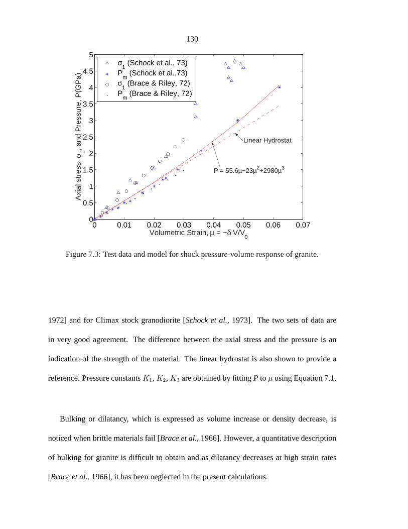
130

0 0.01 0.02 0.03 0.04 0.05 0.06 0.070

0.5

1

1.5

2

2.5

3

3.5

4

4.5

5

Volumetric Strain, µ = −δ V/V0

Axi

al s

tres

s, σ

1, and

Pre

ssur

e, P

(GP

a)

P = 55.6µ−23µ2+2980µ3

Linear Hydrostat

σ1 (Schock et al., 73)

Pm

(Schock et al.,73)σ

1 (Brace & Riley, 72)

Pm

(Brace & Riley, 72)

Figure 7.3: Test data and model for shock pressure-volume response of granite.

1972] and for Climax stock granodiorite [Schock et al., 1973]. The two sets of data are

in very good agreement. The difference between the axial stress and the pressure is an

indication of the strength of the material. The linear hydrostat is also shown to provide a

reference. Pressure constantsK1, K2, K3 are obtained by fittingP to µ using Equation 7.1.

Bulking or dilatancy, which is expressed as volume increase or density decrease, is

noticed when brittle materials fail [Brace et al., 1966]. However, a quantitative description

of bulking for granite is difficult to obtain and as dilatancy decreases at high strain rates

[Brace et al., 1966], it has been neglected in the present calculations.

131

0 0.5 1 1.5 2 2.5 3 3.5 4 4.50

0.5

1

1.5

2

2.5

3

3.5

4

Pressure,P(GPa)

Equ

ival

ent S

tres

s,σ(

GP

a)HEL

JH−2 model (Intact)

ε = 10−4 s−1.

ε = 105 s−1.

JH−2 model(Fractured)

Fractured

Schock et al. (1973)Ramsey and Chester (2004)

Figure 7.4: Test data and model for strength of intact and damaged granite.

7.3.2 Strength

The HEL is taken as 4.5 GPa, the average value from [Petersen, 1969]. This includes both

the deviatoric stress and the hydrostatic pressure components. To determine the strength

and pressure components, we follow the method described inJohnson and Holmquist

[1999]. The HEL volumetric strain is solved fromHEL, K1, K2, K3, andG asµHEL =

0.045. SubstituteµHEL into Equation 7.1 gives pressure at HEL ofPHEL = 2.73 GPa.

The equivalent stress, defined as twice of the material shear strength, at HEL is 2.66 GPa

(σHEL). The intact equivalent stress of the material as a function of pressure, from data in

Figure 7.3, is shown in Figure 7.4. Also shown is the calculated value from JH-2 model us-

ing constants in Table 7.1 at two strain rates, 105 s−1 and 10−4 s−1. It seems that the effect

of strain rate is rather small. The strain rate coefficient,C, is assumed to be 0.005, taken as

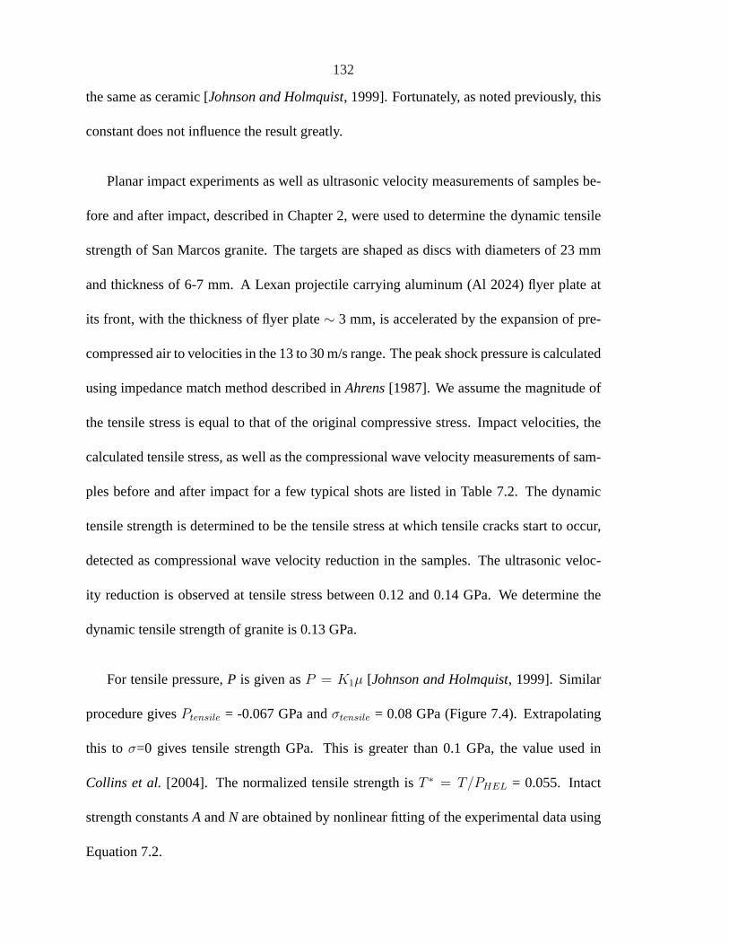
132

the same as ceramic [Johnson and Holmquist, 1999]. Fortunately, as noted previously, this

constant does not influence the result greatly.

Planar impact experiments as well as ultrasonic velocity measurements of samples be-

fore and after impact, described in Chapter 2, were used to determine the dynamic tensile

strength of San Marcos granite. The targets are shaped as discs with diameters of 23 mm

and thickness of 6-7 mm. A Lexan projectile carrying aluminum (Al 2024) flyer plate at

its front, with the thickness of flyer plate∼ 3 mm, is accelerated by the expansion of pre-

compressed air to velocities in the 13 to 30 m/s range. The peak shock pressure is calculated

using impedance match method described inAhrens[1987]. We assume the magnitude of

the tensile stress is equal to that of the original compressive stress. Impact velocities, the

calculated tensile stress, as well as the compressional wave velocity measurements of sam-

ples before and after impact for a few typical shots are listed in Table 7.2. The dynamic

tensile strength is determined to be the tensile stress at which tensile cracks start to occur,

detected as compressional wave velocity reduction in the samples. The ultrasonic veloc-

ity reduction is observed at tensile stress between 0.12 and 0.14 GPa. We determine the

dynamic tensile strength of granite is 0.13 GPa.

For tensile pressure,P is given asP = K1µ [Johnson and Holmquist, 1999]. Similar

procedure givesPtensile = -0.067 GPa andσtensile = 0.08 GPa (Figure 7.4). Extrapolating

this to σ=0 gives tensile strength GPa. This is greater than 0.1 GPa, the value used in

Collins et al. [2004]. The normalized tensile strength isT ∗ = T/PHEL = 0.055. Intact

strength constantsA andN are obtained by nonlinear fitting of the experimental data using

Equation 7.2.

133

Table 7.2: One-dimensional impact parameters, as well as pre- and post-shot compressionalwave velocities for Al2024 flyer plate into San Marcos granite.

Shot Projectile Tensile Pre-shot PostshotVelocity Stress Vp, km/s Vp, km/s 4Vp Comments

m/s MPaGa11 13.5 120.8 6.45 6.45 0% No visible cracksGa7 15.6 140 6.5 5.65 13% Incipient cracks; few well

developed shorter cracksGa1 20 172 6.6 5.56 15.7%Incipient cracks; fairly

well-developed cracks;relatively long spall cracks

Ga3 30 271 6.64 – – Fragmented, not measur-able

No proper fractured strength data for granite are found. Instead, some fractured data

for marble are used for this purpose [Ramsey and Chester, 2004]. Triaxial extension exper-

iments are carried out on Carrara marble to study fracture mechanism in their work. We fit

the data available to Equation 7.3 to obtain the fracture strength constants,B andM.

More experiments for fracture strength of granite are necessary to obtain a better con-

strain of these fractured strength parameters. The normalized fractured strength is limited

not to exceed the maximum fractured strength,σ∗fmax, taken as 0.2 here, or 0.53 GPa as the

equivalent stress.

7.3.3 Damage

Damage (D) describes the transition from intact to fractured strength. Under a constant

pressure, damage begins to accumulate when the material begins to flow plastically (D =

0). When the material is completely damaged,D = 1. The damage parametersD1 andD2

used byJohnson and Holmquist[1999] are not directly measurable. Instead, numerical

adjustment is applied to obtainD1 andD2 listed in Table 7.1.

134

7.3.4 Tensile cracking softening

The maximum principal tensile stress for the tensile softening model is 0.15 GPa, as noted

above. The associated fracture energy is assumed to be 70J/m2, which is the value ob-

tained for ceramics [Clegg and Hayhurst, 1999].

7.4 Examples

Using the JH-2 model parameters for San Marcos granite determined above, several calcu-

lations are performed using finite element/difference package AUTODYN 2D to simulate

impacts with different combinations of projectile and impact velocity. Planar impact of Al

into mm scale San Marcos granite discs as well as impact into 20x20x15 cm granite block

by commercial lead bullet and copper ball are simulated. The impact velocities range from

13 m/s to 1200 m/s. Parameters for projectiles are retrieved from AUTODYN library [AUT,

2003]. The results are presented below and compared with experimental results.

7.4.1 Lead bullet impacting granite

Simulation of shot 117, a 3.2 g lead bullet impacting a 20x20x15 cm granite block at

1200 m/s vertically is carried out and compared with our experimental result. Radius of

the projectile is 3 mm. Figure 7.5a shows the initial setup of the simulation, as well as the

locations of the gauges points used. The geometry of the problem setup and the response of

target are assumed to be axisymmetric. The meshfree Smoothed Particle Hydrodynamics

(SPH) solver [Lucy, 1977;Benz and Asphaug, 1995] is used for the projectile and rock

135

target, with smoothing particle size to be 0.125 mm for the projectile and 0.25 mm for

the rock target. Figure 7.5b plots the peak shock pressure of the gauge points versus the

normalized distance from impact. Exponential fit of the data gives the initial pressure,P0,

as 8.74± 0.56 GPa, which is close to the analytical calculation, 10.3 GPa. The attenuation

coefficient,n is 0.91± 0.1, and this is lower than the predicted value, 1.3 (Chapter 3).

Figure 7.6 illustrates the damage accumulation with time for our simulation. During

the early stage of formation of the impact crater, shear damage caused by shear stress is

dominant near the region around the projectile (Figure 7.6a, b). During the later stage,

failure mechanism changes to principal tensile stress and finger-like tensile cracks began

to grow by the tensile strain localization during expansion of the shock wave (Figure 7.6c).

Finally, large tensile cracks are formed and propagate further into the rock target (Figure

7.6d). The excess damage along the centerline in Figure 7.6d is believed to be caused by

the numerical artifact, which is a very common problem for numerical simulation.

The simulated final damage profile is chosen at the time when no more obvious damage

is produced, and the result is compared with the experimental result. For convenience, cross

section showing different types of cracks and damage depth is shown again (Figure 7.7a).

Asymmetry of cracking pattern in experiment is caused by the heterogeneity of the rock

target. The calculated crater depth is∼ 1.5 cm, and crater diameter is∼ 7 cm (Figure 7.7b),

both of which agree well with the experiment. The prediction of radial tensile cracks with

the experimental result is encouraging: shape and depth of tensile cracks for both situations

are very similar. The tensile cracks extend to 6-7 cm for both cases.

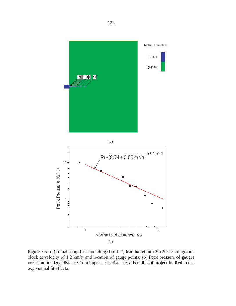
136

(a)

1 10

1

10

Pe

ak P

ressu

re (

GP

a)

Normalized distance, r/a

Pr=(8.74 0.56)*(r/a)+-+--0.91 0.1

(b)

Figure 7.5: (a) Initial setup for simulating shot 117, lead bullet into 20x20x15 cm graniteblock at velocity of 1.2 km/s, and location of gauge points; (b) Peak pressure of gaugesversus normalized distance from impact.r is distance,a is radius of projectile. Red line isexponential fit of data.

137

5 cm

T=0.002 ms

T=0.007 ms

T=0.017 ms

T=0.033 ms

(a)

(b)

(c)

(d)

.

.

Figure 7.6: Simulated damage contour for shot 117 at several times during impact event.(a) and (b): During early stage of impact, damage caused by shear stress dominated highpressure region around projectile; (c) finger-like tensile cracks begin to form due to tensilestrain localization; (d) final profile showing the propagation of tensile cracks.

138

Shear induced damage

Spall cracksCrater depth = 1.5 cm

Radial tensile cracks

Damage depth

6-7 cm

(a)

Crater depth = 1.5 cmCrater diameter 7 cm

Shear induced damage

Spall cracks

Radial tensile cracks

Crack depth

6-7 cm

5 cm

Material status

Void

Hydro

Elastic

Plastic

Bulk Fail

Fail 11

(b)

Figure 7.7: Cross section of granite impacted by lead bullet at 1200 m/s illustrating crackdistribution. Normal impact. (a) Experimental result; (b) AUTODYN-2D simulation at0.03 ms. Left panel illustrates material status; right panel illustrates damage.

139

Shear-induced damageCrater depth

~ 1 cm

5 cm

Crack depth

7 ~ 8 cm

Radial tensile cracks

(a)

Crater depth~ 1 cm

Crater diameter ~ 5 cm

Shear induced damage

Radial tensile cracks

5 cm

Crack depth7 ~ 8 cm

Material status

Void

Hydro

Elastic

Plastic

Bulk Fail

Fail 11

(b)

Figure 7.8: Cross section of granite impacted by copper ball at 690 m/s. Normal impact.(a) experimental result; (b) simulation at 0.04 ms. Others are the same as in Figure 7.7b.

140

7.4.2 Copper ball impacting granite

Shot 1194, impact of a copper ball (0.64 cm in radius) into a 20x20x15 cm San Marcos

granite block at velocity of 690 m/s is simulated. Except for the impact velocity and pro-

jectile material, the simulation setup is the same as that for Shot 117. Figure 7.8 shows the

comparison between the experiment and simulated result. Again, the agreement concern-

ing the crater depth, number of radial tensile cracks as well as the crack shape and depth

between these two is very good. Crater depth is∼ 1 cm, crater diameter is∼ 5 cm (Figure

7.8a, b), and tensile crack depth extends to∼ 8 cm.

7.4.3 Plate impact of Al flyer plate into granite

The four planar impacts of Al flyer plate into granite discs, listed in Table 7.2, are simulated.

Lagrangian solver is used for both the flyer plate and rock target, with uniform cell size

of 0.1 mm. What we measured in experiments is the ultrasonic wave velocity reduction

perpendicular to the impact surface for these samples. The ultrasonic wave velocities are

indirect measurements of damage.

For a fractured body, the ultrasonic velocity reduction would be high compared with

that with few or no cracks. For our one dimensional planar impacts, cracks produced are

mainly oriented parallel with the impact surface. These cracks would reduce ultrasonic

wave velocities measured in the direction perpendicular to the crack orientation [Anderson

et al., 1974]. As will be discussed below, the simulated damage for the four shots correlates

qualitatively well with the ultrasonic wave velocity measurements and the observations of

cracks within the covered samples.

141

Figure 7.9 shows the different degrees of damage for the four impacts. HereD = 0

means intact, andD = 1 means fully fragmented. Crack is not observed for the lowest

velocity impact,U = 13.5 m/s (Figure 7.9a). No velocity reduction is observed from mea-

surements (Table 7.2). With the increase of impact velocity, tensile cracks are developed.

The number of cracks increases with the impact velocity. For the weak-moderate impact

with impact velocity ofU = 15.6 m/s, only incipient and few well-developed shorter cracks

are observed (Figure 7.9b). Long spall crack is seen for the moderate impact with impact

velocity ofU = 20 m/s (Figure 7.9c). The samples still remain contact for both cases (D <

0.5). Compressional wave velocity reduction also increases with the impact velocities (Ta-

ble 7.2). When the impact velocity is as high as 30 m/s, severe damage (D > 0.8) is reached

along the spall plane within the sample (Figure 7.9d). The sample is not measurable for

ultrasonic wave velocities at this stage.

7.4.4 Oblique impact

An oblique impact into a 20x20x15 cm granite, with impact angle at45o, is simulated

using AUTODYN-3D. The projectile is the same as that in Section 7.4.2, and the impact

velocity is 1000 m/s. Figure 7.10 shows the cross section of the recovered target after

being cut open, while Figure 7.11 presents the calculated result for this shot. Asymmetry

is observed on both figures. The pattern of damage and tensile cracks in Figure 7.11 is in

good agreement with the directly measured one (Figure 7.10).

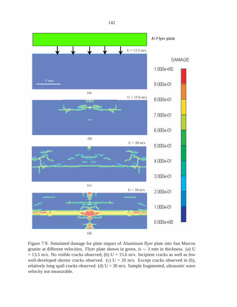
142

(a)

(b)

(c)

(d)

U = 13.5 m/s

U = 15.6 m/s

U = 20 m/s

U = 30 m/s

5 mm

Al Flyer plate

Figure 7.9: Simulated damage for plate impact of Aluminum flyer plate into San Marcosgranite at different velocities. Flyer plate shown in green, is∼ 3 mm in thickness. (a) U= 13.5 m/s. No visible cracks observed; (b) U = 15.6 m/s. Incipient cracks as well as fewwell-developed shorter cracks observed. (c) U = 20 m/s. Except cracks observed in (b),relatively long spall cracks observed. (d) U = 30 m/s. Sample fragmented, ultrasonic wavevelocity not measurable.

143

Impact

5 cm

Figure 7.10: Cross section of granite impacted by copper ball at 1000 m/s, experimentalresult.Vectorshows impact angle at 450. Visible tensile cracks are highlighted.

144

Damage

1.0

0.9

0.8

0.7

0.6

0.5

0.4

0.3

0.2

0.1

0.0

5 cm

Impact

Figure 7.11: Simulated result at 0.1 ms for shot shown in Figure 7.10.

145

5 cm

Material status

Void

Hydro

Elastic

Plastic

Bulk Fail

Fail 11

(a)

20 m

Material status

Void

Hydro

Elastic

Plastic

Bulk Fail

Fail 11

(b)

Figure 7.12: Simulated result shown effect of gravity on formation of tensile cracks. Nor-mal impact. (a) 500g, ap=3 mm; (b) 1g, ap=1500 mm. Left panel illustrates materialstatus, right panel for damage status. Notice different scales on the two plots. See text fordiscussion.

146

7.4.5 Effect of gravity on damage and cracks

Large craters formed in a planetary gravity field can be simulated by much smaller pro-

jectiles at elevated gravity using a geotechnical centrifuge, on the condition that similarity

between the two cases is satisfied [Schmidt and Housen, 1987]. The similarity means that

the product ofG anda should be constant for two impacts, whereG is the planetary gravity,

anda is the projectile radius. Therefore, a large impact with G=1g, whereg is the gravita-

tional constant, and a=1.5 m should be similar with a small scale impact with G=500g, a=3

mm, keeping other impact conditions the same.

The effect of gravity on propagation of cracks is also investigated numerically. The

two impacts mentioned above are simulated using the JH2 model parameters for granite.

The dimension of target is scaled accordingly. For both cases, projectile is lead and impact

velocity is 1200 m/s. Figure 7.12 compares the damage profiles at the final stage. Figure

7.12a has less tensile cracks than Figure 7.12b, especially in the deep region, no obvious

tensile cracks are observed in Figure 7.12a. This phenomenon indicates that existence of

high gravity prevents the propagation of cracks. This can be explained by the relatively

large hydrostatic pressure in the deep depth, which has a negative effect on the propagation

of tensile cracks.

7.5 Conclusion

This work is intended to provide a preliminary quantitative description of response of ge-

ological material to impact loading. The JH-2 constitutive model to describe mechanical

character of brittle material is applied to granite for the first time and is coupled with a ten-

147

sile crack softening model to simulate impacts with different combinations of projectiles

and impact velocities. The strength, pressure and damage characteristics determined either

from direct experimental data, or from indirect numerical calibration, appears to predict

the extent of damage and tensile crack propagation into the rock target to an encouraging

degree. Uncertainties remain regarding the determination of model constants of fracture

strength and energy, indicating that more detailed experimental data of fracture strength of

shock damaged granites are needed.

148

Chapter 8

Future Work

The previous chapters describe systemically our preliminary study of shock-induced dam-

age in rocks and the application to impact cratering. However, there is a very rich field and

a lot of aspects are still to be explored.

Only two types of rocks are used in this study to obtain the scaling relation. Other

typical terrestrial and planetary rocks, such as sandstone, ice, etc, should be included to

have a full coverage of geological materials. Furthermore, multi layer targets, instead of

one single target, should be used to represent the real geological conditions. If possible, the

dimension of both target and projectile should be varied within a much larger range. More

oblique impacts should be carried out, since it is a very interesting field itself and the result

might be very intriguing.

The ultrasonic tomography inversion for the low porosity granite is a big improvement

over the traditional dicing method. But still there is uncertainty with this method and it

is not the most efficient way. In the future, other new method (such as CT inversion) is

suggested to be tried and compared with previous results. The very important yet most

difficult part is to carry out seismic exploration in the field and to build a database of

damage depth for impact craters.

149

It is also true that a lot of questions are left unexplored in the field of simulation. For

example, different strength models should be tested and compared for San Marcos granite

and more static mechanical experiments be carried out to reduce the error of the determined

model parameters. Simulation for other geological materials should also be initiated.

150

Bibliography

(2003), Autodyn theory manual,Century Dynamics Inc.

Ackermann, H. D., R. H. Godson, and J. S. Watkins (1975), A seismic refraction technique

used for subsurface investigations at meteor crater, arizona,J. Geophys. Res, 80, 765–

775.

Ahrens, T., and J. O’Keefe (1987), Impact on the earth, ocean, and atmosphere,Int. J.

Impact Eng., 5, 13–32.

Ahrens, T. J. (1987), Shock wave techniques for geophysics and planetary physics, inMeth-

ods of experimental physics, edited by C. G. Sammis and T. L. Henyey, pp. 185–235,

Academic Press, San Diego.

Ahrens, T. J., and J. V. G. Gregson (1964), Shock compression of crustal rocks; data for

quartz, calcite and plagioclase rocks,J. Geophys. Res, 69, 4839–4874.

Ahrens, T. J., and A. M. Rubin (1993), Impact-induced tensional failure in rock,J. Geo-

phys. Res, 98, 1185–1203.

Ai, H. A., and T. J. Ahrens (2004), Dynamic tensile strength of terrestrial rocks and appli-

cation to impact cratering,Meteoritics and Planetary Science, 39(2), 233–246.

151

Anderson, D. L., B. Minster, and D. Cole (1974), The effect of oriented cracks on seismic

velocities,J. Geophys. Res., 79, 4,011–4,015.

Ashby, M., and C. Sammis (1990), The damage mechanics of brittle solids in compression,

Pure Appl. Geophys., 133, 489–521.

Baldwin, E., L. Vocadlo, and I. Crawford (2005), Validation of autodyn in replicating large-

scale planetary impact events,LPSC 36th abstract, p. 1380.

Bate, M., and A. Burkert (1997), Resolution requirements for smoothed particle hydrdy-

namics calculations with self-gravity,Mon. Not. R. Astron. Soc., 288, 8060–8073.

Benz, W., and E. Asphaug (1995), Simulations of brittle solids using smooth particle hy-

drodynamics,Computer physics communications, 87, 253–265.

Berge, P. A., J. G. Berryman, and B. P. Bonner (1993), Influence of microstructure on rock

elastic properties,Geophys. Res. Letter, 4, 2619–2622.

Birch, F. (1960), The velocity of compression waves in rocks to 10 kilobars,J. Geophys.

Res., 65, 1083–1102.

Brace, W., and D. Riley (1972), Uniaxial deformation of 15 rocks to 30 kb,Int. J. Rock.

Mech. Min. Sci., 9, 271–288.

Brace, W., B. P. Jr, and C. Scholz (1966), Dilatancy in the fracture of crystalline rocks,J.

Geophys. Res., 71, 3939–3953.

Carter, W. J. (1978), Explosively produced fracture of oil shale,Progress Report LA-7357-

PR, Los Alamos:, Los Alamos National Laboratory.

152

Clegg, R., and C. Hayhurst (1999), Numerical modeling of the compressive and tensile

response of brittle materials under high pressure dynamic loading, inShock compression

of condensed matter–1999, edited by M. Furnish, L. Chhabildas, and R. Hixson, pp.

321–324, American Institute of Physics, New York.

Cohn, S. N., and T. J. Ahrens (1981), Dynamic tensile strength of lunar rock types,J.

Geophys. Res., 86, 1,794–1,802.

Collins, G., J. Melosh, and B. Ivanov (2004), Modeling damage and deformation in impact

simulations,Meteoritics & Planetary Science, 39, 217–231.

Dahl, J., and P. Schultz (2001), Measurement of stress wave asymmetries in hypervelocity

projectile impact experiments,Int. J. Impact Eng., 26, 145–155.

Fujiwara, A. (1980), On the mechanism of catastrophic destruction of minor planets by

high-velocity impact,Icarus, 31, 277–288.

Gault, D. (1978), Experimental studies of oblique impacts,Proc. Lunar Planet. Sci. Conf.,

9, 3843–3875.

Gilbert, G. (1893), The moons’s surface, a study of the origin of its features,Bull. Philos.

Soc. Wash., 12, 241–292.

Grady, D., and M. Kipp (1987), Dynamic rock fragmentation, inFracture mechanics of

rocks, edited by B. Atkinson, pp. 429–475, Academic press, San Diego, California.

Grady, D. E. (1998), Shock-wave compression of brittle solids,Mechanics of Materials,

29, 181–203.

153

Grady, D. E., and R. E. Hollenbach (1979), Dynamic fracture strength of rock,Geophys.

Res. Lett., 6, 73–76.

Grady, D. E., and L. Lipkin (1980), Criteria for impulsive rock fracture,Geophys. Res.

Lett., 7, 255–258.

Heinrich, K. (1991),Ultrasonics fundamentals and applications, Elsevier Science publish-

ers LTD, New York.

Hole, J. A. (1992), Nonlinear high-resolution three-dimensional seismic travel time tomog-

raphy,J. Geophys. Res., 97, 6553–6562.

Holsapple, K. A. (1993), The scaling of impact processes in planetary sciences,Annu. Rev.

Earth Planet. Sci., 21, 333–73.

Holsapple, K. A., and R. M. Schmidt (1982), On the scaling of crater dimensions 2. impact

processes,J. Geophys. Res., 87, 1849–1870.

Housen, K. R., and K. A. Holsapple (1990), On the fragmentation of asteroids and planetary

satellites,Icarus, 84, 226–253.

Housen, K. R., R. M. Schmidt, and K. A. Holsapple (1983), Crater ejecta scaling laws:

fundamental forms based on dimensional analysis,J. Geophys. Res., 88, 2485–2499.

Hudson, J. A. (1990), Overall elastic properties of isotropic materials with arbitrary distri-

bution of circular cracks,Geophys. J. R. Astron. Soc., 102, 465–469.

Johnson, G., and T. Holmquist (1999), Response of boron carbide subjected to large strains,

high strain rates, and high pressures,J. Applied Phys., 85, 8060–8073.

154

Johnston, D. H., M. N. Toksoz, and A. Timur (1979), Attenuation of seismic waves in dry

and saturated rocks: Ii. mechanisms,Geophysics, 44, 691–711.

Kachanov, M. (1993), Elastic solids with many cracks and related problems,Adv. Appl.

Mech., 30, 259–445.

Kadono, T., and A. Fujiwara (2005), Cavity and crater depth in hypervelocity impact,Int.

J. Impact Eng., 31, 1309–1317.

King, M. S. (2002), Elastic wave propagation in and permeability for rocks with multiple

parallel fractures,Int. J. Rock Mech. Min Sci., 39, 1033–1043.

Lange, M. A., and T. J. Ahrens (1983), The dynamic tensile strength of ice and ice-silicate

mixtures,J. Geophys. Res., 88, 1197–1208.

Lange, M. A., T. J. Ahrens, and M. B. Boslough (1984), Impact-cratering and spall fracture

of gabbro,Icarus, 58, 383–395.

Levin, V., and M. Markvo (2005), Elastic properties of inhomogeneous transversely

isotropic rocks,Int. J. Solids and Structures, 42, 393–408.

Liu, C., and T. J. Ahrens (1997), Stress wave attenuation in shock-damaged rock,J. Geo-

phys. Res., 102, 5243–5250.

Lockner, D. (1995), Rock failure, inRock physics and phase relations: A handbook of

physical constants, edited by T. Ahrens, pp. 127–147, American Geophysical Union,

Washington DC.

155

Love, S. G., F. Horz, and D. E. Brownlee (1993), Target porosity effects in impact cratering

and collisional disruption,Icarus, 105, 216–224.

Lucy, L. (1977), A numerical approach to the testing of the fission hypothesis,Astron. J.,

82, 1013–1024.

Matsui, T., and H. Mizutani (1977), Why is a minor planet minor,Nature, 270, 506–507.

McQueen, R. G., S. P. Marsh, and J. N. Fritz (1967), Hugoniot equation of state of twelve

rocks,J. Geophys. Res., 72, 4999–5036.

Melosh, H. J. (1989),Impact cratering, A Geological process, Oxford Univ. Press, New

York.

Menke, W. (1989),Geophysical data analysis: Discrete inverse theory, Academic Press,

San Diego.

Monaghan, J. (1992), Smooth particle hydrodynamics,Ann. Rev. Astron. Astrophys., 30,

543–574.

Murri, W. J., C. Young, D. A. Shockey, R. E. Tokheim, and D. R. Curran (1977), Deter-

mination of dynamic fracture parameters for oil shale,Report PYD-5046, final report to

Sandia Laboratories, Standford Research Institute.

Nishizawa, O. (1982), Seismic velocity anisotropy in a medium containing oriented cracks-

transversely isotropic case,J. Phys. Earth., 30, 331–347.

Nur, A. (1971), Effects of stress on velocity anisotropy in rocks with cracks,J. Geophys.

Res., 76, 2022–2034.

156

O’Connell, R. J., and B. Budiansky (1974), Seismic velocities in dry and saturated cracked

solids,J. Geophys. Res., 79, 5412–5426.

O’Keefe, J., S. Stewart, M. Lainhart, and T. Ahrens (2001), Damage and rock-volatile

mixture effects on impact crater formation,Int. J. Impact Eng., 26, 543–553.

O’Keefe, J. D., and T. J. Ahrens (1976), Impact ejecta on the moon, inProceeding of 7th

Lunar and Planetary Science Confence, pp. 3,007–3,025.

O’Keefe, J. D., and T. J. Ahrens (1981), Impact cratering: The effect of crustal strength

and planetary gravity,Revs. of Geophys. Space Phys., 19, 1–12.

Payne, J. (1965), Impacts of spherical projectiles of aluminum, stainless steel, titanium,

magnesium, and lead into semi-infinite targets of aluminum and stainless steel,Report

AEDC-TR-65-34, Arnold Eng. Develop. Center, Arnold Air Force Sta. Tenn.

Petersen, C. (1969), Shock wave studies of selected rocks, Ph.D. thesis, Stanford Univer-

sity.

Pierazzo, E., and J. Melosh (2000), Understanding oblique impacts from experiments, ob-

servations, and modeling,Annu. Rev. Earth Planet. Sci., 28, 141–167.

Pilkington, M., and R. Grieve (1992), The geophysical signature of terrestrial impact

craters,Review of Geophysics, 30, 161–181.

Pohl, J., D. Stoffler, H. Gall, and K. Ernstson (1977), The ries impact crater, inImpact and

Explosion Cratering, edited by D. J. R. et al., pp. 343–404, Pergamon, New York.

157

Polanskey, C. A., and T. J. Ahrens (1990), Impact spallation experiments: fracture patterns

and spall velocities,Icarus, 87, 140–155.

Ramsey, J., and F. Chester (2004), Hybrid fracture and the transition from extension frac-

ture to shear fracture,Nature, 428, 63–66.

Roddy, D. J., S. H. Schuster, K. N. Kreyenhagen, and D. L. Orphal (1980), Computer code

simulations of the formation of meteor crater, arizona: Calculations mc-1 and mc-2, in

Proc. Lunar Planet. Sci. Conf., vol. 11, pp. 2,275–2,308.

Schmidt, R. M., and K. R. Housen (1987), Some recent advances in the scaling of impact

and explosion cratering,Int. J. Impact Engeg., 5, 543–560.

Schock, R., H. Heard, and D. Stephens (1973), Stress-strain behavior of a granodiorite and

two graywackes on compression to 20 kilobars,J. Geophys. Res., 78, 5922–5941.

Schultz, P., and R. Anderson (1996), Asymmetry of the mansion impact structure:evidence

for impact angle and direction,GSA Special Paper, 302, 397–417.

Schultz, P., and S. D’Hondt (1996), Cretaceous-tertiary (chicxulub) impact angle and its

consequences,Geology, 24, 963–967.

Shibuya, T., and I. Nakahara (1968), The semi-infinite body subjected to a concentrated

impact load on the surface,Bulletin of JSME, 11, 983–992.

Shipman, F. H., V. G. Gregson, and A. Jones (1971), A shock wave study of coconino

sandstone,NASA Report CR-1842.

158

Shoemaker, E. (1962), Interpretation of lunar craters, inPhysics and Astronomy of the

Moon, edited by Z. Kopal, pp. 283–359, Academic Press, New York.

Shoemaker, E. M. (1963), Impact mechanics at meteor crater, arizona,4, 301–336.

Simmons, G., T. Todd, and H. Wang (1973), The 25-km discontinuity: Implications for

lunar history,Science, 182, 158–161.

Singh, M. M. (1989), Strength of rock, inPhysical properties of rocks and minerals, vol. 2,

edited by Y. S. Touloukian, W. R. Judd, and R. F. Roy, pp. 83–122, Hemisphere Publish-

ing Corporation, New York.

Tompkins, M. J., and N. I. Christensen (2001), Ultrasonic p- and s-wave attenuation in

oceanic basalt,Geophys. Int., 145, 172–186.

Vidale, J. E. (1990), Finite-difference calculation of traveltimes in three dimensions,Geo-

physics, 55, 521–526.

Weidner, D. J. (1987), Elastic properties of rocks and minerals, inMethods of experimental

physics, edited by C. Sammis and T. Henyey, pp. 1–28, Academic press, San Diego,

California.

Wepfer, W., and N. Christensen (1990), Compressional wave attenuation in oceanic basalts,

J. Geophys. Res., 95, 17,431–17,439.

Winkler, K., and T. Plona (1982), Technique for measuring ultrosonic velocity and attenu-

ation spectra in rocks under pressure,J. Geophys. Res., 87, 10,776–10,780.

159

Xia, K., and T. J. Ahrens (2001), Impact induced damage beneath craters,Geophysical

Research Letters, 28, 3525–3527.