Selecting a Centrifugal Pump by System Analysis

PDHonline Course M128 (4 PDH)

Selecting a Centrifugal Pump by System Analysis

2012

Instructor: Randall W. Whitesides, PE

PDH Online | PDH Center5272 Meadow Estates Drive

Fairfax, VA 22030-6658Phone & Fax: 703-988-0088

www.PDHonline.orgwww.PDHcenter.com

An Approved Continuing Education Provider

http://www.PDHonline.org

http://www.PDHcenter.com

www.PDHcenter.com PDH Course M128 www.PDHonline.org

Selecting a Centrifugal Pump by System Analysis © 2003, 2008 Randall W. Whitesides, CPE, PE

1

Selecting a Centrifugal Pump by System Analysis Copyright © 2003, 2008

Randall W. Whitesides, P.E.

Outline/Scope/Introduction Man’s day to day reliance on pumps is inescapable. From confined space automotive

applications to mammoth systems in industrial facilities, fluids are transferred by pumps to and from and through the systems that are now taken for granted as part of our daily lives. Needless to say, a huge amount of energy is expended in accomplishing these pumping tasks. It has been estimated that a large constituent of total industrial power consumption can be attributed to the operation of rotating equipment, the majority of which are pumps. For this reason it is important to insure that these processes, both large and small, are carried out efficiently. Faced with costly power, it makes little sense to select and size a pump by “guessing” how effectively this pump will operate within a system. This course will look at one method of pump sizing that considers the pump’s interrelationship with the system that it is expected to operate efficiently within.

Overview – The System Approach

It is an established fact that a centrifugal pump will operate at the point of intersection of the

impeller characteristic curve and the system curve. Also known is the fact mathematical expressions that define these curves can be established. It therefore stands to reason that the simultaneous solution of these two expressions would result in a numerical demarcation of the pump’s expected operation point. This is the basis for this course. In order to limit the length of this course, the examples and illustrations employed utilize ideal, static systems. It can not be over emphasized that real world systems exhibit variability and that the range of fluid levels, pressures, temperatures, etc., in any given system must be taken into full consideration in order to ascertain the most demanding hydraulic scenario. This comprehensive approach will preclude an over-simplistic analysis that can result in problems. The manual techniques presented in this course are regularly featured as an automated function in any of a number of commercially available hydraulic software products. However, it is important to have a complete understanding of the mechanics that are the basis of this analysis



2

regardless of the format elected, i.e., manual or computerized. A reasonably accurate piping system design and layout must be complete and available to the Engineer before any attempt is made to determine the actual operational point of a centrifugal pump, irrespective of the analytical vehicle employed. While commercially available hydraulic software can perform impressively, the fact remains that the quality of the input data ultimately determines the merit of the overall analysis. This course is formed of two major parts. The first part deals with the impeller characteristic curve. This curve is plotted on the pump manufacturer’s performance curve for a given pump and it shows the relationship between the head and capacity (flow rate) of a given pump/impeller combination. The second part deals with what is commonly referred to as the system curve. It depicts a system’s piping circuit resistance to flow at various flow rates. This curve is not presented on the pump manufacturer’s performance curve because each piping system is unique and totally independent of the pump’s manufactured performance. In brief, the characteristic curve is equipment dependent, the system curve is equipment independent. Before mathematical modeling of curves is undertaken, an explanation of performance curves will be presented and an examination of classical pump selection methods will be provided.

FIGURE 1 –TYPICAL PUMP PERFORMANCE CURVE



3

Pump Performance Curves Pump performance curves are generated by conducting water tests on pump and impeller combinations. The presentation of the test data is somewhat standardized on a rectangular coordinate plane with the x-axis representing capacity and the y-axis representing head. A typical manufacturer’s pump performance curve is shown in Figure 1. It is generally a composite presen-tation of several impeller characteristic curves. In addition to capacity and head data, information for efficiency, brake horsepower, and Net Positive Suction Head Required are also generally plotted on the performance curve. This abundance of hydraulic data all simultaneously displayed on the same coordinate plane can be somewhat intimidating to the first time user of the curves.

Selecting and Sizing a Centrifugal Pump The actual methods of arriving at the final style and size of a centrifugal pump vary widely. If the entire system is well defined with one set of constant operating conditions, then sizing a pump is a straightforward, simple process involving fluid dynamics fundamentals. The design flow rate in many cases is predetermined by process requirements. Since the required pressure to overcome the various heads and to provide this design flow rate is readily estimated, too often the pump selection and sizing routine can unfortunately occur somewhat in this fashion: Selection and Sizing – Assuming Stead State Conditions

1. An estimate of the maximum flow and head requirement is obtained through an abbreviated analysis of a process or system whose design is incomplete. To this estimate a margin (maybe as much as 25%) is added to provide a safety factor;

2. The flow and head values from Step 1, along with other pertinent information, are provided to the pump manufacturer’s representative for a price quotation. The sales representative adds an additional 5% safety factor, selects a suitable pump and impeller size based on efficiency, and sizes a motor so that an overload condition will not occur in case the pump operates “out-on-the-end” of the selected characteristic curve. This completes the selection process;

3. The Engineer receives a pump performance curve from the sales representative as part of the pump purchase. It merely reiterates the head and flow values estimated in Steps 1 and 2 by marking their location on the selected pump’s performance curve with a small right angle symbol (see the illustration on the next page).



4

In some instances the pump installed by this selection process is much too large for the actual system conditions. This necessitates the introduction of artificial resistance in the discharge piping in order to tame the pump’s head or flow, or both. Unfortunately, much of the installed power is wasted as unnecessary energy to compensate for the excessive margin that was originally assumed. Moreover, many processes are not steady-state but rather transient. Many processes operate over a range of conditions and requirements. Embracing an assumption of a steady-state process in these circumstances is a

flawed methodology. Hopefully, the information presented below will prevent such an outcome.

The Case for Math versus Graphics

In order to fully analyze centrifugal pump process systems, we need equations that describe the impeller diameter characteristic and a curve known as the system curve. Engineers have long used mathematical techniques to approximate experimental observations and empirical measurements. This process is known by various phrases some of which are:

1. Numerical modeling; 2. Least squares analysis; 3. Mathematical “smoothing” of data points and; 4. Curve fitting.

The process may not necessarily result in a curvilinear representation. In the field of

statistics, the process is called regression analysis wherein a population of raw data is reduced to a useful mathematical function. A multitude of statistical software applications are commercially available to perform this function. It will be shown momentarily however, that plain old math can be successfully used to “model” a centrifugal pump’s performance and determine the point of operation. Because the techniques are relatively easy, this numerical method is far superior to the alternative graphical method which can only produce an estimate of operation point by approximation from the pump performance curve.



5

The Impeller Characteristic Curve

The impeller characteristic curve is a plot of a specific impeller’s head versus capacity relationship within a given pump housing while pumping water. Referring back to Figure 1 on page 2, we see that this particular pump casing can accept impeller diameters as small as 9 inches and as large as 13 inches. In this case, they are depicted as a “family” of essentially parallel curves. Pump head and capacity are typically represented by the letters H and Q, respectively. From this point forward, the impeller characteristic curve will be referred to as the H-Q curve. Note: All of the curves presented in the example diagrammatic performance curves here are merely schematic in nature.

H–Q Curve Stability

H-Q curves fall into two defining categories: (1) Stable, and (2) Unstable:

FIGURE 2 – STABLE H-Q CURVE FIGURE 3 –UNSTABLE H-Q CURVE Theoretically, with the H-Q curve shown in Figure 3, a pump could have the same head at two or more capacities. This is highly unlikely in any practical sense. In reality, pump and impeller design combinations whose tests reveal excessive unstable operation are generally not brought to market. While there has been mention in the open technical literature about unstable impeller designs, in practical experience impellers whose characteristic results in less head at shut-off (Q = 0) than at some positive capacity, are rarely ever encountered. See Figure 3. Mentioned in



6

conjunction with unstable characteristics are impellers that have been designed for maximum flow per inch of impeller diameter or pumps with a low head coefficient. This concept was first expounded by German Engineer C. Pfieiderer in 1932. Unstable H-Q curves have also been referred to as “drooping curves” and pumps that could possibly exhibit this characteristic would be better suited to non-throttling applications in which the capacity would never be expected to go below a point corresponding to the “peak” of the H-Q curve. Types of Stable H-Q Curves Stable H-Q curves can be (1) Steadily decaying; (2) Steeply sloping and; (3) Relatively flat:

FIG. 4 – STEADILY FIG. 5 – STEEPLY FIG. 6 – RELATIVELY DECAYING H-Q CURVE SLOPING H-Q CURVE FLAT H-Q CURVE

The steadily decaying H-Q curve (Figure 4) is the one that is most frequently encountered. It exhibits a falling head-capacity characteristic in which the head diminishes continuously as the capacity is increased. The best efficiency point usually occurs somewhere between 15 and 20% below shut-off. This characteristic offers very stable pump operation.

The steeply sloping curve (Figure 5) is one where there is a large decrease in head between

that developed at shut-off and that developed far-field. Obviously, this type of H-Q characteristic is best suited for applications where minimum capacity change is desired with resulting large pressure changes.

The relatively flat H-Q curve (Figure 6) refers to a characteristic in which the head changes minimally with changes in the pump’s capacity. If a process requires nearly constant pressure



7

conditions while wide fluctuations in capacity occur, this is the pump/impeller combination that should be sought. Defining the H-Q Curve Mathematically It has been shown that the typical H-Q curve takes the form of a parabolic-type power function in the form,

y x nn= >, where 0 [1] Rewriting this expression in the hydraulic form yields,

H Qn= [2]

For all practical purposes, the head and capacity of a centrifugal pump can be considered to vary parabolically and usually can be represented by a quadratic expression in the standard form,

y ax bx c= + +2 [3]

Rewriting in the hydraulic form yields,

H aQ bQ c= + +2 [4] Now, before we develop more equations, let’s take a look at some x-y coordinate pairs along a typical H-Q curve and convert this data into a mathematical relationship that defines the H-Q curve.



8

FIGURE 7 – H-Q CURVE FOR EXAMPLE 1

EXAMPLE 1 H-Q Curve Fit Given: A low head, very high capacity horizontal split-case 30 x 24 – 30, 880 rpm centrifugal pump in cooling water service, contains a 26½ inch diameter impeller. An H-Q curve schematic with capacity and head data (Q,H) is shown in Figure 7 above. Find: The quadratic equation that defines the H-Q curve for this pump and impeller. Solution: A normal, steadily decaying impeller characteristic curve with performance data at three separate operating points is provided. We can define the H-Q curve with as little as three data pairs (coordinates) using Equation [4] on page 7. Now, an ingenious utility avails itself when one of the three data points is purposely taken a the shut-off condition (i.e. Q = 0 ). The need for the solution of three simultaneous equations, expressed in terms of head and capacity, is reduced to two equations because,

with thenQ H aQ bQ c= = + +0 2 ( ) ( )becomes H a b c= + +0 02 [5]

and ∴ =H c which states that the constant c in Equations [4] and [5] is always equal to the pump’s shut-off head:



9

[ ]H cat shut- off = [6] In our first example then, c = 186 feet. The remaining coefficients, a and b, can be determined by substituting this value of c along with the other x-y coordinate pairs, i.e. midpoint (20,000 gpm, 155 feet) and endpoint (30,000 gpm, 115 feet) into forms of Equation [4], and solving the two resulting equations simultaneously,

[ ][ ]

H aQ bQ c

H aQ bQ c

= + +

= + +

2

2

midpoint

endpoint

Substituting,

( ) ( )155 20 000 20 000 1862= + +a b, , [7]

( ) ( )115 30 000 30 000 1862= + +a b, , [8]

Rearranging [7] and defining a in terms of b: ab

=− −31 20 000

4 108,

x

Substituting this expression for a into [8]: ( )11531 20 000

4 109 10 30 000 1868

8=− −

+ +

,,

bb

xx

And solving for b: b = −8 33 10 5. x

Substituting the value for b into [7]: ( ) ( )( )155 4 10 8 33 10 20 000 1868 5= + +−a x x. , Results in the value: a = − −8 2 10 8. x Therefore, the H-Q curve for the Example 1 pump and impeller is described by the mathematical expression:

H Q x Q= − + +− −8 2 10 8 33 10 1868 2 5. .x [9]

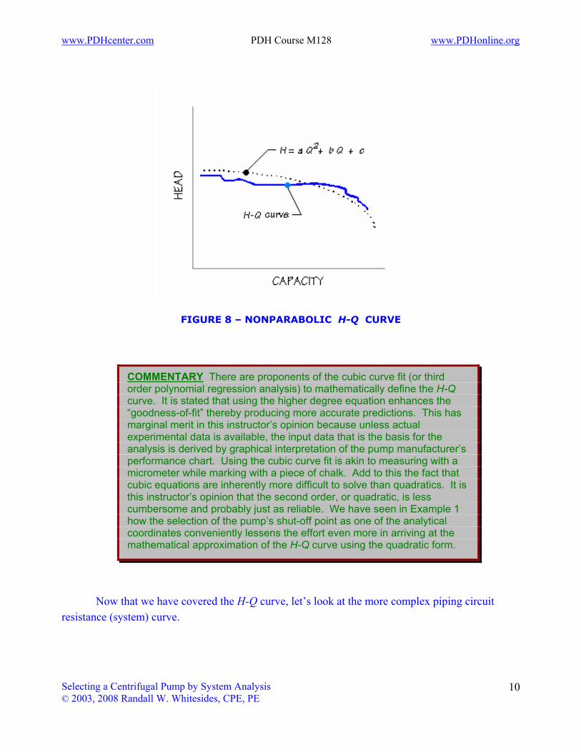
Using just ordinary algebra, the method just outlined eliminates the need for a larger number or higher order of equations or solutions to arrive at the mathematical equivalent of the H-Q curve. Only in the event that it is apparent that the H-Q curve is erratic or widely divergent from the parabolic (see Figure 8) would a more sophisticated routine or regression analysis be justified.



10

FIGURE 8 – NONPARABOLIC H-Q CURVE

Now that we have covered the H-Q curve, let’s look at the more complex piping circuit resistance (system) curve.

COMMENTARY There are proponents of the cubic curve fit (or third order polynomial regression analysis) to mathematically define the H-Q curve. It is stated that using the higher degree equation enhances the “goodness-of-fit” thereby producing more accurate predictions. This has marginal merit in this instructor’s opinion because unless actual experimental data is available, the input data that is the basis for the analysis is derived by graphical interpretation of the pump manufacturer’s performance chart. Using the cubic curve fit is akin to measuring with a micrometer while marking with a piece of chalk. Add to this the fact that cubic equations are inherently more difficult to solve than quadratics. It is this instructor’s opinion that the second order, or quadratic, is less cumbersome and probably just as reliable. We have seen in Example 1 how the selection of the pump’s shut-off point as one of the analytical coordinates conveniently lessens the effort even more in arriving at the mathematical approximation of the H-Q curve using the quadratic form.



11

The System Curve

The system curve is the relationship between total head loss (HL) and flow rate; the curve itself appears as a steadily rising quadratic function because it is formed by the increasing resistance of the piping circuit that occurs with increasing flow rate. The diagram shown here is a schematic of a typical system curve.

With good reason, note that the parameter Q will now be labeled as flow rate in lieu of capacity. When discussing pump performance the interest lies in head and capacity; when discussing the system curve the interest lies in frictional head loss associated with flow rate. Make no mistake, the quantity Q, volumetric flow rate, is identical for both concepts and remains unchanged in the context of either analysis.

System heads fall into two categories: (1) flow dependent and (2) flow independent. Either head may be constant or variable depending upon the system. Flow dependent head is simply frictional resistance head. All systems contain flow dependent head. Flow independent head can include items such as static discharge head or residual pressure at the discharge point. Examples of flow independent (constant pressure) head are pumps pumping liquid from a low elevation to a higher elevation or pumps pumping into a process vessel with constant back-pressure, see Figure 9.

FIGURE 9 – STATIC DISCHARGE HEAD/CONSTANT PRESSURE HEAD



12

Static head and constant pressure will be denoted as HS; its value falls on the vertical axis of the pump performance curve and it determines the relative origin (or y-intercept) of the frictional head loss curve. Figure 10 shows a process in which there is a pressure constant. Figure 11 shows a process in which there is no pressure constant.

FIGURE 10 FIGURE 11

When visualizing a system curve, it is convenient to think of the pump’s discharge as being throttled with a globe or other valve. If the pump were allowed to operate through a fully open valve with no piping or fittings connected, the operation point would be at the run-out point indicated by point 1 in Figure 12 on page 13. As the valve is closed, the system resistance is increased and the operation point begins to “move-up” the H-Q curve to point 2. Finally, with the valve fully closed there exists no flow and the pump is said to be operating at shut-off, point 3.



13

FIGURE 12 – PUMP SYSTEM WITH THROTTLED DISCHARGE

Exactly What is a Pump System? For the purposes of hydraulic analysis, a pump system is,

any defined set of single or multiple variable fluidic or physical

conditions or static arrangements, a pump can in combination encounter, that will affect its performance.

ADDITIONAL INFORMATION Most of the inefficient heat associated with the delivery of energy to the pumped fluid is normally carried away by the fluid stream. A centrifugal pump operating at shut-off does not have benefit of this inherent heat dissipation feature. For this reason, there exists a distinct probability of pump over-heating with prolonged periods of operation at or near shut-off conditions.



14

For example, a simple change in a pumped liquid’s temperature from 60EF to 100EF, all other process conditions remaining unchanged, would analytically constitute two separate and distinct systems. Would a simple change like this warrant analytical merit? It would depend completely on the criticality and accuracy desired from the analysis. Consideration for variations in process temperature are important because temperature directly affects fluid viscosity and vapor pressure, which in turn affect frictional losses and static heads. Temperature also affects fluid density which affects the developed pressure and the required brake horsepower. Therefore, a structured evaluation of the total system must be made to accurately develop a system curve. The system curve determines exactly where the pump will operate along the H-Q curve and therefore it should always be used to dictate the pump selection. In order to fully evaluate the suitability of a given pump, the system curve must be developed for minimum, normal, and maximum process conditions anticipated. System curve development is also the best technique to evaluate the performance impact to the multitude of contingencies and various equipment combinations that can be, or could in the future be, contained in a process piping system. In this respect, a good example of contingency analysis could involve the aging of a piping system. For instance, the performance of a given pump could be predicted at some point in the future by developing a system curve that would represent an estimate of reduction in the internal diameter and increased roughness due to scaling or encrustation over time. The system curve can be difficult to model because the discharge piping circuit can consist of many branches of the same or differing nominal sizes, each of which can contain many components. Practically, pumps operate singly, in parallel, and in series. In the interest of brevity, no attempt will be made to explain, analyze, or investigate, the myriad of piping systems variations to which a pump can be connected. In order to efficiently present the concept of hydraulic system analysis within a sensible course scope, an example will be limited to a single centrifugal pump operating within a single pipe circuit. The hydraulic analysis knowledge associated with compound pump operation and multiple branch flows is well established and, in many cases, is incorporated into the software products previously mentioned. Before we can mathematically define the system curve we must develop it. This entails locating x-y coordinate pairs (flow rate, head loss) that a given system generates on the pump performance coordinate plane that will “form” the curve. A minimum of three points, or coordinate pairs, is required to adequately mathematically define a system curve.



15

Before we can progress any further, we must broach the concept of the fluid friction factor (f ).

A Crash Course in Friction Factors

The friction factor is a critical variable regardless of the technique employed to determine frictional head loss. It is therefore important to have a background knowledge of its history and development.

During the 1880s an Irish Engineer and physicist named Osbourne Reynolds conducted experiments by visually monitoring flow patterns in glass tubes with dye injected fluids. His observations resulted in the now famous dimensionless quantity which bears his name, the Reynolds number, Re. The

Reynolds number relates the physical and geometric properties of fluid density, velocity, viscosity, and pipe diameter. Essentially, flows were shown to be: Laminar (smooth) for Re < 2,000; Transitional for 2,000 < Re < 4,000; and Turbulent for Re > 4,000

In 1938 British Engineer C.F. Colebrook demonstrated that for Re > 3,000, a fluid friction factor existed which was a function of both the value of Re and the relative roughness (,/D) of the pipe. No approximations here; the Colebrook factor is extremely accurate. The Colebrook friction factor is defined as:

1

237

2 51f D R fe

= − +

log

..ε

[10]

This hideous looking mathematical creature is implicit in f which requires an iterative process for convergence to a solution. Going forward, a host of later experimental Engineers developed approximations of this friction factor concept that were explicit in f, culminating in a graphical representation of a friction factor relationship produced by L.F. Moody in 1944. A schematic diagram of what has become to be known as the Moody chart is shown in Figure 13.

f



16

FIGURE 13 – MOODY FRICTION FACTOR CHART

The Moody chart was used extensively prior to the advent of the programmable calculator and the desktop computer. While the Moody chart provides a more simple method of f determination, an extension of a concept derived from the Moody chart can be used to rid us of the burden of evaluating f at each flow rate. The Moody chart f values become asymptotic (f .constant) in the zone of complete turbulence. With a close examination of the Moody chart, and using water as the fluid, a fully turbulent fluid flow friction factor can be shown to approximately vary with pipe diameter in accordance with,



17

TABLE 1 - APPROXIMATE ASYMPTOTIC MOODY FRICTION FACTORS FOR

CLEAN COMMERCIAL STEEL PIPE WITH FLOW IN ZONE OF COMPLETE TURBULENCE

Nominal Size (in) 1 2 3 4 6 8-10 12-16 18-24 30-48

Friction Factor (f ) 0.023 0.019 0.018 0.017 0.015 0.014 0.013 0.012 0.011

A great deal of technical literature is available, in print and on the internet, on the subject of computing system friction. Any of this information can be successfully employed depending upon the student’s preference, past experience, and applicability to the system and liquid being considered. Since nearly all practical process applications fall in the fully turbulent flow regime, and in order to establish a common source of f values in this course, we will use the approximate values of f shown in Table 1 above for the examples and quiz questions that will follow. Frictional head losses are attributable to:

1. Contractions and expansions; 2. Process equipment such as heat exchangers and filters; 3. Valves and pipe fittings; and 4. Straight line length friction.

In all cases, the line losses vary directly as a function of the square of the mean fluid

velocity (HF % V2). Let’s look at one of the more common frictional head loss equations, the Darcy-Weisbach formula:

H fLD

VgF =2

2 [11]

Where, f = Moody (or Colebrook) friction factor L = pipe line length, feet V = mean fluid velocity, ft/sec D = inside pipe diameter, feet g = gravitational constant, ft/sec²



18

Without derivation, the Darcy-Weisbach frictional head loss formula can be rewritten in terms of flow rate Q to appear as:

Hf L Q

dFE= 0 0311

2

5. [12]

Where, f = Moody (or Colebrook) friction factor LE = pipe line equivalent length, feet Q = flow rate, gpm d = inside pipe diameter, inches

Since in reality, piping systems can vary in diameter, and branches may exist, it will usually be necessary to sum several fluid frictional resistances. A detailed example of this analytical process will not be provided here; however, the basic methodology is:

1. Using an accurate piping arrangement drawing, or unfortunately a piping diagram if that is all that is available, divide the system into identifiable sections with each section having a single pipe size and a single flow rate. In other words, do not include as an analytical section a 3 inch pipe flowing 75 gallons per minute with a downstream 3 inch branch flowing 85 gallons per minute.

2. Determine the total equivalent length (LE) of each section by summing the component equivalent lengths and straight pipe lengths.

SCOPE REFINEMENT There are two schools of thought on the basis of accounting for pipe and component resistance to fluid flow. Basically these are: (1) Equivalent length (LE), and (2) Resistance coefficient (K). In many cases the two methods are used simultaneously depending on the components contained in the piping system. In the interest of brevity, and to concentrate on the subject at hand, there is no intention to digress into a lengthy discourse of the merits of each. Suffice it to say that pipe line resistance, both straight line lengths and piping components, can be accurately represented by either method. For no particular reason, the former basis (LE) has been chosen to display in the formulas, equations, and descriptions presented here.



19

3. Calculate the fluid frictional head loss for each section based on the equivalent length, the diameter, and the flow rate of that section (use the modified Darcy formula, Equation [12]). And finally,

4. Determine the total fluid frictional head loss for the path or branch being analyzed by summing the sectional fluid frictional head losses for all of the sections that form that path.

Total head loss (HL ) at any given point along the system curve is the sum of static and constant pressure heads and frictional head at that point (see Figure 14),

H H HL S F= + [13]

FIGURE 14 – COMPONENT HEADS SUMMATION

Let’s look a step-wise approach to develop a single system curve and then view an example:

1. In order to establish the origin of the frictional head loss curve, the flow independent heads must be determined. The pump’s physical elevational relationship to supply and destination liquid levels must be established as well as the identification of any constant pressure discharge or suction conditions. This will locate the first system curve coordinate pair, (0, HS). Refer to Figure 14.



20

2. Next, two quantities that represent flow dependent head must be located. Remember, flow dependent head is friction head resulting from liquid movement. Since the system curve must be fully defined throughout the entire anticipated flow rate range, two logical points to examine would be normal and maximum anticipated flow rates. Compute the frictional head loss (HF) associated with each of the selected flow rates.

3. To evaluate the two additional coordinate pairs that will complete the system curve, separately add the frictional head losses determined in Step 2 to the flow independent head (HS) determined in Step 1.

Defining the System Curve Mathematically We know that a coordinate pair on the system curve will be located at any arbitrarily selected flow rate (Q) and the corresponding total head loss (HL ) associated with that flow rate. We also know that the frictional loss constituent of HL is defined by Equation [12] which is repeated here:

Hf L Q

dFE= 0 0311

2

5.

For our purpose in this course, we can assume that all of the components of the right side of the equation are constant, with the exception of flow rate Q. In order to simplify our analytical task, we can therefore group all of the constants and set them equal to a quantity we will call K:

Kf L

dE=

0 03115

. [14]

Accordingly, by substitution we can rewrite Equation [12] to appear as,

H KQF = 2 [15] and simply evaluate K for the system constants of friction factor, pipe equivalent length, and pipe diameter that exist. It also logically follows that the total head loss associated with any and all selected fully turbulent flow rates would take on the form of a rewrite of Equation [13],

H KQ HL S= +2 [16]



21

Now let’s take a look at a real life example of the mathematics we just covered. From this example we will determine the value of K of a system and thereby produce a mathematical relationship that defines the system curve.

EXAMPLE 2 System Curve Development and Curve Fit Given: The 36 inch diameter piping system to which the EXAMPLE 1 pump is connected has a calculated equivalent length of 21,729 feet. The system exhibits no flow independent head losses. Assume that Table 1 approximate friction factor values are acceptable to develop head loss data. Find: The quadratic equation that defines the system curve. Solution: We are given: d = 36 inches; LE = 21,729 feet; Static head = constant pressure head = HS = 0. Next: referring to Table 1 on page 17 indicates that for d = 36, the approximate friction factor f = 0.011. By using Equation [14] the value of K can be determined to be,

( )( )( )K

f Ld

E= = = −0 0311 0 0311 0 011 21 72936

123 105 57. . . ,

. x

Since in this case HS = 0, from Equation [16] the system curve for EXAMPLE 2 is described by the mathematical expression:

H KQ H

H QL S

L

= +

= +−

2

7 2123 10 0. x

H QL = −123 10 7 2. x [17] The system curve for this example is illustrated in Figure 15 on the following page.



22

FIGURE 15 – EXAMPLE 2 SYSTEM CURVE

Determining the Centrifugal Pump’s Operating Point

At the beginning of the course we stated that a centrifugal pump will operate at the point of intersection of the impeller characteristic curve and the system curve. Also stated was the fact that if mathematical expressions that define these two curves could be found, we could solve the resulting equations simultaneously and analytically determine this operation point. We are now ready to carry out this final aspect of the system analysis. Solving Simultaneous Equations In our case we are involved with two quadratic equations with two variables (called unknowns). To solve a pair of simultaneous equations means to find all of the sets of values of the unknowns which, when substituted in the original equations, will satisfy both the equations at the same time; hence the term simultaneous. You may recall that the solutions of simultaneous equations are known as roots of the equations and that there will be a root for each degree, or order, of the equation. Here again, in our case we will actually determine two roots only one of which will



23

be the realistic operating point of the centrifugal pump. The best way to demonstrate this procedure is to continue with our previous example pump and system and determine its operating point.

EXAMPLE 3 Determination of Pump Operation Point Given: The EXAMPLE 1 pump connected and operating in the EXAMPLE 2 system. Find: The true operation point. In other words, determine what capacity and what total dynamic head the pump in EXAMPLE 1 will produce when connected to the system of EXAMPLE 2. Solution: We will solve the H-Q curve quadratic equation we developed in EXAMPLE 1 simultaneously with the system curve quadratic equation we developed in EXAMPLE 2. Graphically this appears as,

FIGURE 16 – PUMP HEAD AVAILABLE AND PUMP HEAD REQUIRED

There are multiple methods to solve simultaneous equations. Rest assured, those straight-forward techniques of addition, subtraction, and completing the square that you probably recall from algebra are not suitable for the negative fractional and infinitesimal coefficients that have been generated from our analysis. We will be relegated to the methods of substitution and the quadratic formula,



24

xb b ac

ax

b b aca1

2

2

242

42

=− + −

=− − −

, [18]

The units of the ordinate (vertical) axis of the pump performance curve are feet of head of pumped liquid. This axis represents both feet of head available (H) as well as feet of head required (HL ). This leads us to the fact that,

H HL≡ [ ]at the point of operation [19]

And allows us to solve Equations [9] and [17] simultaneously thusly,

H Q x Q= − + +− −8 2 10 8 33 10 1868 2 5. .x [9] H QL = −123 10 7 2. x [17]

Since H ≡ HL, we can set the above equations equal to each other,

− + + =− −8 2 10 8 33 10 1868 2 5. .x Q x Q 123 10 7 2. x − Q Gathering like quantities and converting the expression into the standard quadratic form results in,

2 05 10 8 33 10 186 07 2 5. .x − −− − =Q x Q [20] where, a = 2.05 x 10-7 b = -8.33 x 10-5 c = -186 x = Q

We can now use the quadratic formula, Equation [18], to solve for the values of Q,

( ) ( )( )( )( )( )Q

b b aca1

2 5 9 7

7

42

8 33 10 6 94 10 4 2 05 10 186

2 2 05 1030 326=

− + −=

− − + − −=

− − −

−

. . .

.,

x x x

xgpm



25

( ) ( )( )( )( )( )Q

b b aca2

2 5 9 7

7

42

8 33 10 6 94 10 4 2 05 10 186

2 2 05 1029 919=

− − −=

− − − − −= −

− − −

−

. . .

.,

x x x

xgpm

As stated, because a quadratic (second order) equation has two roots, we are presented with two capacities. Q2 is known as an extraneous root because it is obviously meaningless from a practical standpoint. Therefore, the true operating capacity of the EXAMPLE 1 pump in the EXAMPLE 2 system is 30,326 gpm. Now that we have determined the system operating capacity, we can determine the corresponding system operating head by simply substituting this value of Q into either of the simultaneous equations. For convenience, we should select Equation [17] because it is easier to evaluate:

( )( )H QL = = =− −123 10 123 10 30 326 1137 2 7 2. . ,x x feet

A good check is to calculate the head by evaluating the second simultaneous equation. The result should be the same. What we have just ascertained would appear graphically as,

FIGURE 17 – EXAMPLE 3 POINT OF OPERATION



26

Conclusion In the beginning of the course, a selection and sizing method was outlined that made the case of the steady-state assumption in a transient process. As is true with many topics, there are simple, but unfortunately, incorrect methods of performing analysis. The correct method to size a centrifugal pump is presented in the following step-by-step procedure: Comprehensive Method of Selection and Size

1. Using the normal or average flow and head requirement of the process or system obtained from a careful and considered process study, make a tentative size selection from a pump manufacturer’s graphical coverage chart (or map) of all available sizes;

2. Superimpose the system curve, preferably mathematically, or alternatively graphically, on the performance curve of the tentatively selected pump from Step 1;

3. Select the impeller size and speed to match the intersection of the system curve. Generate additional system curves that represent minimum and maximum flows and/or changes in static fluid levels so that the performance of the impeller size selected for normal conditions can be evaluated over the entire anticipated operating range;

4. Check to insure that ample margin exists between Net Positive Suction Head Available and Net Positive Suction Head Required at the various operating points;

5. Estimate the pump’s efficiency at the operation point determined in Step 3 and calculate the power requirements;

6. Repeat the above procedure for larger and smaller pumps in the vicinity of the tentative pump selection to compare efficiency at the normal operation point;

7. Make the final selection based on a life-cycle cost analysis comparison of each pump considered in Step 6 that efficiently satisfies the process requirements.

Step 2 is critical in the pump selection process above.

Summary 1. Pump impeller characteristic (H-Q) curves and piping circuit resistance (system) curves can be mathematically defined and simultaneously solved to arrive at the true operating point(s) of a centrifugal pump. This fact is at the heart of a pump system analysis; 2. We are all challenged to use our available resources as efficiently as possible. Forcing an assumed steady-state system analysis on a transient operating system often results in a simple, incorrect, energy inefficient, pump selection and size; 3. A systems analysis approach that accounts for all of the requirements and varabilities for a specific application or process should always dictate the pump selection.

Selecting a Centrifugal Pump by System Analysis

Documents

Transcript of Selecting a Centrifugal Pump by System Analysis