SEEING THE SALT IN THE LAURENTIAN BASIN USING

COMBINED GRAVITY AND SEISMIC DATA

Senior Thesis

Submitted in partial fulfillment of the requirements for the

Bachelor of Science Degree

At The Ohio State University

By

Jack M. Pelishek

The Ohio State University

2017

ii

i

TA B L E O F CO N TE N TS

Abstract…………………………………………………………………………..iii

Acknowledgements……………………………………………………………… iv

List of Figures………………………………………………………………….... v

Introduction……………………………………………………………………… 1

Geologic Setting

Study Area…………………………….…….……………..……………. 5

Hydrocarbon Potential and Stratigraphy………………………………... 7

Methods

Bureau Gravimétrique International Database (BGI)…………………... 9

OM Gravity Modelling…………………………………………………..10

OpendTect Seismic Viewer…..………………………………………….11

Results

OM Gravity Maps………………………………………………………..13

Comparing the Free-air Gravity Anomalies with Seismic Reflection Lines

#21 & #5…...15

Comparing the Free-air Gravity Anomalies with Seismic Reflection Lines

#3 & #4……22

Discussion

Understanding the Gravity Response of Salt…………………………… 28

Additional Salt Bodies on Seismic Reflection Lines #1, #6, #20, & #29..28

Plotting of Salt Bodies on Google Earth ……....………………………. 32

The Laurentian Fan ……………………………………………………. 35

Conclusions…………………………………………………………………….. 38

Suggestions for Future Research……………………………………………….. 39

ii

References Cited….……….……………………………………………………. 40

iii

ABSTRACT

Integration of gravity anomaly data with seismic reflection profiles lowers exploration risk and

enhances the geologic interpretation of the subsurface. This project focused on pinpointing the

location of marine salt domes within Canada’s Laurentian Basin. Salt domes concentrate

hydrocarbons in about 50% of the world’s basins, so studying salt behavior is critical in

understanding the mechanisms of the Laurentian petroleum system. Combined seismic and

gravity studies are effective for mapping salt bodies because of the large respective velocity and

density variations of the subsurface that they provide. This study considers their application in

the largely unexplored Laurentian Basin that holds deep-water Mesozoic salt domes related to

the Triassic extension of the Atlantic Ocean. In particular, multiple possible salt bodies imaged

on 29 lines of full stack 2D seismic reflection data with OpendTect-software processing were

compared with gridded free-air gravity anomalies processed by Geosoft’s Oasis montaj software.

The analysis suggested that the pattern of strongly negative gravity anomalies may reflect

Triassic structures delineated along several seismic lines. Furthermore, the seismic data reveals

a drop in bathymetry into the Laurentian Fan, which lies in the southeastern part of the gravity

grid marked by strong positive anomalies. Accordingly, given its analogy with the divergent

margins of the hydrocarbon-rich Brazilian and Angolan Basins, the Laurentian Basin will

continue to be of exploration interest to the hydrocarbon industry.

iv

ACKNOWLEDGEMENTS

I would like to thank my research advisor Dr. von Frese for advising me on this project. I

learned a lot from his gravity and magnetics courses, which sparked my interest for taking on

this project. I also would like to thank Dr. Asgharzadeh, a former student of Dr. von Frese now

at Tehran University who has been researching the Laurentian Basin and directed me to the

appropriate resources and data. In addition, Dr. Afif Saad’s publications on using potential field

methods to further constrain salt dome mapping were indispensable to the success of my project.

Furthermore, I thank Dr. Darrah, who made field camp an enjoyable experience and he always

extended a helping hand on those hot days in Ephraim. He also mentors me in regards to oil and

gas career advice. Dr. Sawyer was one of the first professors I met at the School of Earth

Sciences, and after taking his reflection seismology course I felt like a true geoscientist in the

making. Dr. Sawyer aided me in interpreting the seismic profile and acquiring the appropriate

software. Lastly, I would like to thank Shell Exploration and Production Company for funding

my research in the SURE program.

Elements of this research were presented at The Ohio State University’s 2017 Fall

Undergraduate Research Forum and the 2017 Shell Undergraduate Research Experience poster

session.

v

LIST OF FIGURES

1. A comparison of a low gravity signal side by side with a salt dome on seismic data.

2. Seismic profile reprinted from Asgharzadeh et al. (2017).

3. Overall Geology of the Canadian Atlantic Margin.

4. Google Earth view of Canadian Atlantic Margin.

5. Stratigraphic Chart of the Laurentian Basin.

6. OM Database Window containing raw data in headers.

7. Free-air Gravity Anomaly Grid in its simplest form.

8. Free-air Gravity Anomaly Map with seismic lines #21 and #5 drawn in.

9. Seismic Line #21 viewed with OpendTect, but without interpretation.

10. Seismic Line #21 Profile Path.

11. Profile Database of Line #21.

12. Seismic Line #21 Gravity Profile.

13. Seismic Line #21 with annotation.

14. Seismic Line #5 Profile Path.

15. Seismic Line #5 Gravity Profile.

16. Seismic Line #5.

17. Seismic Line #3 Profile Path.

18. Profile Database of Line #3.

19. Seismic Line #3.

20. Seismic Line #3 Gravity Profile.

21. Seismic Line #4 Profile Path.

22. Seismic Line #4.

23. Seismic Line #4 Gravity Profile.

24. Salt Bodies (initial 6) plotted on Free-air Gravity Anomaly Map

25. Seismic Line #1.

26. Seismic Line #6.

27. Seismic Line #20.

28. Seismic Line #29.

29. Salt Bodies (all 14) plotted on Google Earth.

30. Salt Bodies (all 14) plotted on Free-air Gravity Anomaly Map.

vi

31. Seismic Line #5 annotated to emphasize the drop in bathymetry into the Laurentian Fan.

32. Free-air Gravity Anomaly Map displaying the continental edge of the Laurentian Fan.

1

INTRODUCTION

The integration of gravity data with seismic data to explore for hydrocarbons is a

relatively modern approach in the energy industry. Companies such as GEOSOFT and Statoil

have established this technique with proven success in areas such as Brazil, West Africa, the

North Sea, and Gabon [Chandler and Burns, 2015]. The fundamental logic in incorporating

gravity data with seismic data is that a synergy can be achieved to reduce geologic complexity

and improve subsurface resolution of the basin [Saad, 1993]. In hydrocarbon exploration,

gravity data are second only to seismic reflection data, because the potential field data provide

additional clues about the existence of faults, anticlines, intrusives, and salt domes [Chandler

and Burns, 2015]. In particular, this project focused primarily on locating potential salt domes

on seismic reflection profiles and then evaluating their gravity response to strengthen the

hypothesis of the salt body’s existence. The rule of thumb is that a gravity minimum marks a

salt structure in the subsurface, whereas a gravity maximum would indicate lithology that is

denser than salt [Chandler and Burns, 2015]. Figure 1 exhibits an example of this correlation of

geophysical signals from Saad (1993).

The Laurentian Basin is located offshore of eastern Canada. It was chosen for this study

because the seismic reflection data were available through an academic license and the presence

of salt bodies and gravity data had been established by Asgharzadeh et al. (2017) as shown in

Figure 2. This figure was a major influence on the project because I wanted to uncover more

details about this and other salt bodies in the seismic dataset.

The overall goal of this research project is to constrain the seismic interpretation with

gravity modeling for enhanced subsurface analysis of the basin, evaluate the basin’s hydrocarbon

2

potential, and map the salt domes. The initial effort focused on displaying multiple 2D seismic

reflection profiles to analyze the stratigraphy and hydrocarbon traps of the basin. A grid of free-

air gravity anomalies (in mGal) was established next to constrain the subsurface details of the

salt structures. Finally, the distribution of salt domes was evaluated along multiple seismic

reflection lines using the available free-air gravity constraints.

Salt has a pressure-wave velocity of 4,500 m/s and a uniform, low density ~2,165 kg/𝑚3

that contrasts negatively to that of the basaltic and sedimentary rock components of the

bathymetry. Thus, this density contrast should yield a pattern of relatively negative free-air

anomaly values over salt bodies.

3

Figure 1. Correlation of a minimum gravity anomaly with the seismic reflection response for a salt

dome. Adapted from Saad (1993).

4

Figure 2. Seismic profile adapted from Asgharzadeh et al. (2017).

5

GEOLOGIC SETTING

Study Area

The Laurentian Basin is a deepwater Mesozoic basin that covers 60,000 square

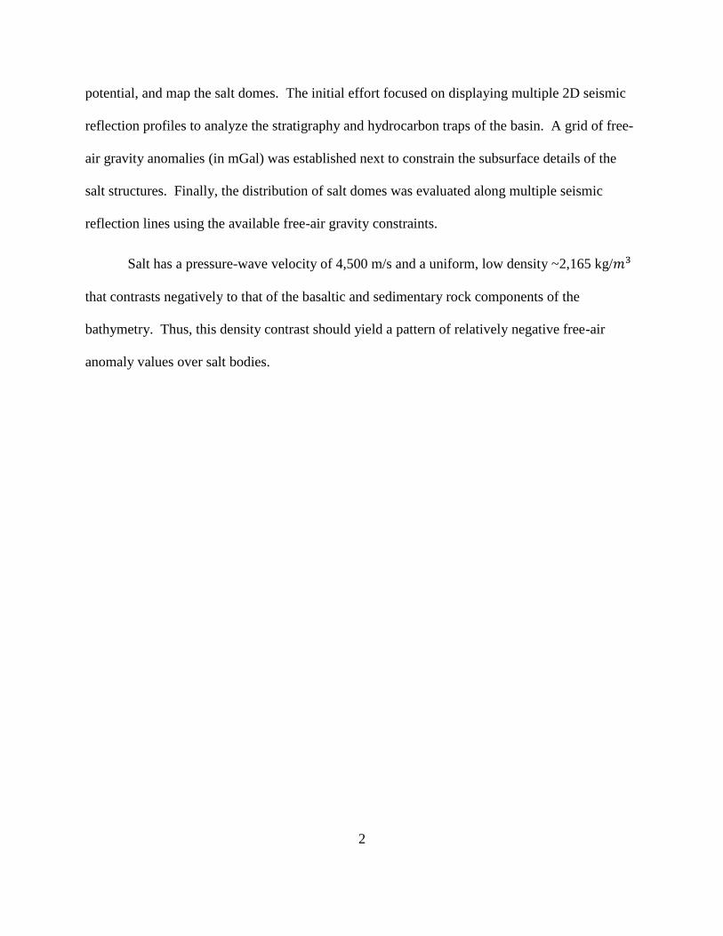
kilometers, located east of Nova Scotia and south of Newfoundland (Figure 3). This figure was

annotated with an orange rectangle to denote the approximate location of the seismic survey,

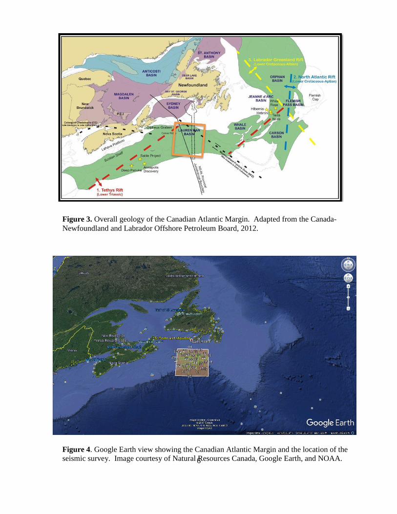
which is also shown from a Google Earth image perspective (Figure 4). To the west of the

Laurentian Basin lies the Scotian Shelf on an extensional margin, and to the East are the Grand

Banks on an extensional/strike-slip margin [Hogg and Enachescu, 2007]. The regional geology,

featuring extensional structures and interconnected rift basins, can be traced back to the late

Triassic split of North America and Africa. Likewise, the Triassic split accounts for the

Laurentian Basin’s divergent setting [Canada-Newfoundland and Labrador Offshore Petroleum

Board, 2012]. The basin also displays salt tectonics similar to the hydrocarbon-rich Brazilian

and Angolan margins. Salt of approximately 3 km of thickness was deposited in interconnected

rifts during the late Triassic [Adam and Krézek, 2012].

6

Figure 3. Overall geology of the Canadian Atlantic Margin. Adapted from the Canada-

Newfoundland and Labrador Offshore Petroleum Board, 2012.

Figure 4. Google Earth view showing the Canadian Atlantic Margin and the location of the

seismic survey. Image courtesy of Natural Resources Canada, Google Earth, and NOAA.

7

Hydrocarbon Potential and Stratigraphy

The Laurentian basin is classified as a deepwater basin, with water depths ranging from

480m to 3,750m [Canada-Newfoundland and Labrador Offshore Petroleum Board, 2012]. It is

estimated to contain 600-700 million barrels of oil and 8-9 Tcf of natural gas, yet the basin has

remain relatively unexplored due to governmental disputes [Fagan and Enachescu, 2007]. A dry

well (Bandol #1) was drilled in 2001 through a joint venture of ExxonMobil, Murphy Oil, and

Gulf Canada. Industrial optimism remains because of the encouraging seismic mapping and the

consistently producing Jeanne d’Arc basin to the northeast [Hogg and Enachescu, 2007].

The basin’s infill consists mainly of Jurassic-to-Tertiary clastics and carbonates, along

with high-porosity and high-permeability sandstone reservoir rocks [Canada-Newfoundland and

Labrador Offshore Petroleum Board, 2012]. Its hydrocarbon potential is reinforced by the

presence of salt domes that can concentrate the hydrocarbons. In particular, salt domes are

estimated to have sealed around 50% of the world’s oil reserves. As the renowned German

geologist Carl Ochsensius put it back in 1888: “the origin of petroleum… is always intimately

connected with salt districts” [Jackson and Hudec, 2017]. Figure 5 shows the stratigraphy of the

Laurentian Basin, where the Jurassic-to-Cretaceous were especially important periods of salt

deformation [Canada-Newfoundland and Labrador Offshore Petroleum Board, 2012].

8

.

Figure 5. Stratigraphic chart of the Laurentian Basin. Reprinted from the Canada-

Newfoundland and Labrador Offshore Petroleum Board (2012).

9

METHODS

Gravity data were obtained from the Bureau Gravimétrique International database

(http://bgi.omp.obs-mip.fr/data-products/Gravity-Databases) for the area 44N - 46N and 56W

- 58W of the seismic survey. GEOSOFT’s Oasis montaj (OM) software was used to grid the

gravity data onto a base map and produce high-resolution free-air gravity anomaly maps. The

seismic reflection data were viewed using the OpendTect seismic software and accessed with

their Open Seismic Repository from

(https://www.opendtect.org/osr/Main/LaurentianBasinCanada). Some 29 lines of full stack 2D

data were extracted that had been collected in 1984 and subsequently reprocessed in 2006.

Bureau Gravimétrique International Database (BGI)

Gravity data are free to download for educators and researchers from agencies such as

NOAA, NASA, USGS, European Space Agency, and BGI. The BGI office is located in Paris

and was established by the International Union of Geodesy (IUGG), with additional support from

13 universities and laboratories. It is one of the most prominent earth gravity databases because

of its comprehensive globe-spanning land, marine, and airborne data. Most importantly, BGI

readily redistributes their data to university researchers and students. This project first extracted

the free-air gravity anomalies (FAGA) of the Laurentian Basin from the BGI marine gravity

database, which required entering the following inputs: Data Type (= sea), Minimum Latitude (=

44), Maximum Latitude (= 46), Minimum Longitude (= -58), and Maximum Longitude (= -56).

These marine gravity anomalies are derived from the BGI’s version of the standard EGM08

model that includes shipborne FAGA estimates from the Eigen-6c4 model [Asgharzadeh et al,

10

2017]. After the appropriate inputs were entered, BGI’s website returned an ASCII file of the

FAGA values for download and submission to OM processing.

OM Gravity Modelling

For OM processing, the raw ASCII file was uploaded into the project database. Manual

adjustments included defining the coordinate projection. The longitude channel (X) was set to

LONGITUDE and the latitude channel (Y) was set to LATITUDE. Next, the local datum was

selected to establish the dataset’s location on the globe. The standard datum for North American

datasets is set by the 1983 North American datum (NAD83) [Hinze et al., 2013]. Next, a new

projected (x,y) coordinate system was defined. Here, the new X-channel was set as UTME_N83

and the Y-channel set to UTMN_N83. OM now displays the gravity file in an Excel-like

spreadsheet (Figure 6). From left to right the column headers read “Longitude,” “Latitude,”

“Anomaly_mgal_,” “UTMN_N83,” and “UTME_N83,” for generating the gravity grids. At

each (x,y) location on the grid, there is an associated anomaly value in mGal. The software

displays the variation of these values by assigning each value a color, and the end result is the

gridded FAGA data superimposed onto a base map. This gravity map displays colored spatial

variations that reflect geologically significant variations of subsurface density. OM’s algorithm

for generating the gridded FAGA values in mGals is derived from

𝑔𝐹𝐴𝐺𝐴= 𝑔𝑜𝑏𝑠 - 𝑔∅ + 0.3086*h (1)

where 𝑔𝑜𝑏𝑠 is the observed gravity value, 𝑔∅ is the latitude correction, h is the elevation

difference in feet, and the scalar is the free-air correction. This equation takes into account the

latitudinal change in gravity, and is equivalent to the Bouger gravity anomaly on the ocean

11

surface [Hinze et al., 2013]. Lastly, OM was used to obtain profile plots of the FAGA to locate

the gravity anomaly minima along spatial traverses.

OpendTect Seismic Viewer

Seismic data are expensive to obtain and thus typically remains proprietary information

within the oil and gas companies that collected the data. Fortunately, OpendTect provided no-

cost access to the Laurentian seismic reflection data archived at the Open Seismic Repository

and Natural Resources Canada. Some 29 lines of full stack 2D reflection data collected in 1984

and reprocessed by Western Geophysical in 2006 were successfully loaded into OpendTect6.0

Figure 6. OM’s Database Window that shows how the raw data are

compiled into headers before transformed into a grid.

12

for processing. Specifically, the NRCAN_Laurentian_Basin file was downloaded and used as

the survey data root to define the rectangular box of the survey with fixed in-line range, cross-

line range, and bin size parameters. Next, the 2D viewer was used to display the seismic array of

any one of the 29 lines desired. This project display used the default “seismics” color scheme of

red, brown, and white to enhance the seismic waveform. The user can also zoom in on the

profiles to examine the geology on different scales. The zoom function was particularly useful to

delineate the salt bodies in seismic line #21 and reveal the basin’s complexity in seismic line #5.

13

RESULTS

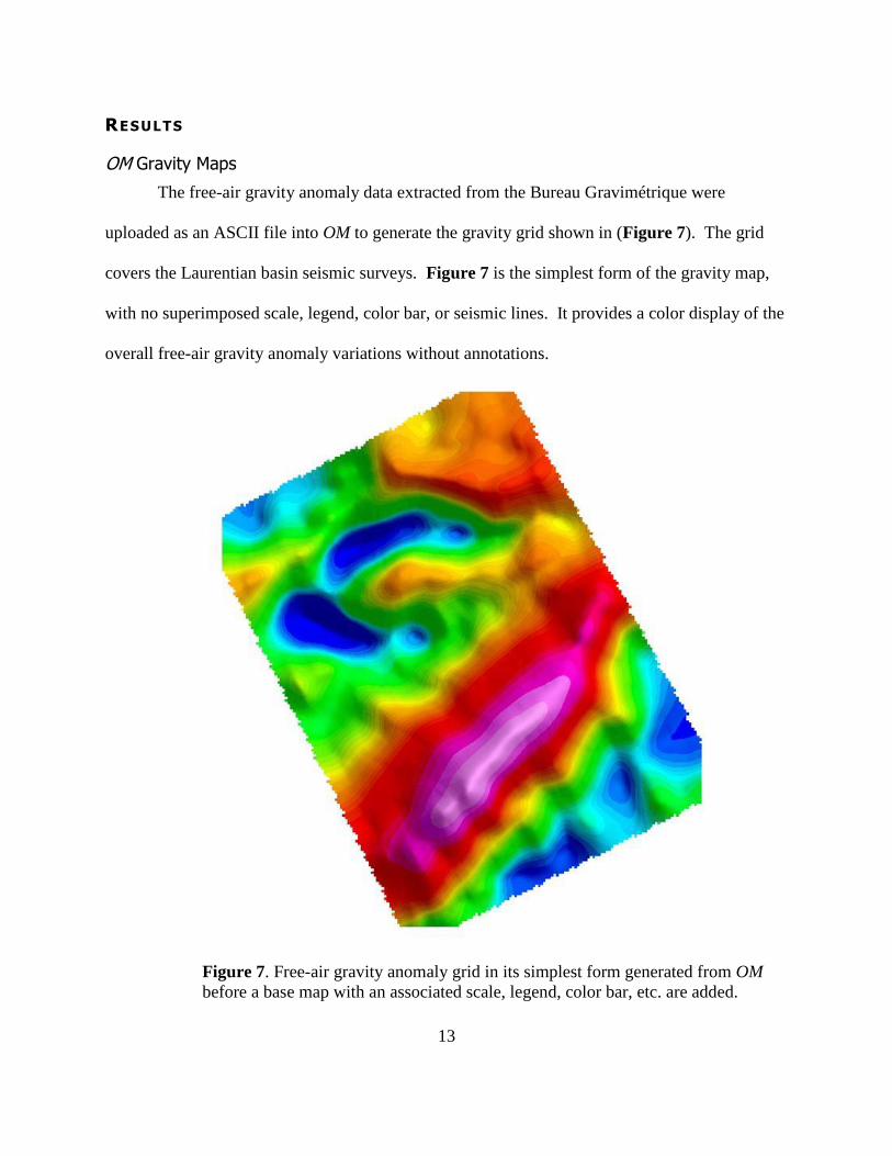
OM Gravity Maps

The free-air gravity anomaly data extracted from the Bureau Gravimétrique were

uploaded as an ASCII file into OM to generate the gravity grid shown in (Figure 7). The grid

covers the Laurentian basin seismic surveys. Figure 7 is the simplest form of the gravity map,

with no superimposed scale, legend, color bar, or seismic lines. It provides a color display of the

overall free-air gravity anomaly variations without annotations.

Figure 7. Free-air gravity anomaly grid in its simplest form generated from OM

before a base map with an associated scale, legend, color bar, etc. are added.

14

The base map was constructed next to provide a scale, legend, color bar, and other

interpretational information on the gravity values. In particular, seismic lines #5 and #21 were

critical to the result of this project, and thus they were plotted onto the map to reveal their

possible correlations with the gravity anomalies. An especially prominent feature of Figure 8 is

the horseshoe-shape minimum anomaly in the upper left portion of the map. These strong

negative anomalies range from -30.0 mGal to -37.9 mGal. Also, the southernmost area of line #5

crosses over a strong positive gravity anomaly with a maximum amplitude of 55 mGal.

Figure 8. Free-air gravity anomaly map with superimposed seismic reflection lines #21 and #5.

15

Comparing the Free-air Gravity Anomalies with Seismic Reflection Lines #21 & #5

The 29 lines of full stack 2D seismic reflection data collected in 1984 (and reprocessed in

2006) were successfully loaded into the OpendTect viewing software to investigate the basin’s

stratigraphy and hydrocarbon traps. In particular, Figure 9 displays the seismic reflection line

#21 which intersects the closed free-air gravity anomaly minimum in Figure 8 that Asgharzadeh

et al. (2017) have attributed to the subsurface presence of a salt dome.

Figure 9. Seismic reflection line #21 running from SW (left) to NE (right) and

viewed with OpendTect samples a closed free-air gravity anomaly minimum in

Figure 8 that was attributed to the presence of a salt dome [Asgharzadeh et al.,

2017] as highlighted in Figure 13.

16

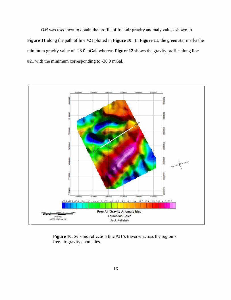
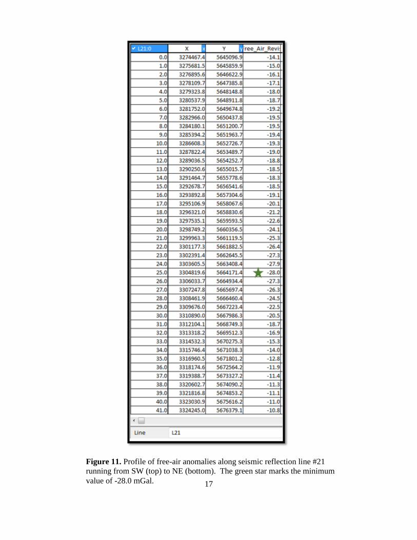
OM was used next to obtain the profile of free-air gravity anomaly values shown in

Figure 11 along the path of line #21 plotted in Figure 10. In Figure 11, the green star marks the

minimum gravity value of -28.0 mGal, whereas Figure 12 shows the gravity profile along line

#21 with the minimum corresponding to -28.0 mGal.

Figure 10. Seismic reflection line #21’s traverse across the region’s

free-air gravity anomalies.

17

Figure 11. Profile of free-air anomalies along seismic reflection line #21

running from SW (top) to NE (bottom). The green star marks the minimum

value of -28.0 mGal.

18

Figure 12. Gravity profile along seismic reflection line #21 running from SW (left)

to NE (right). The green arrow pinpoints the minimum value of -28.0 mGal.

Figure 13. Seismic reflection line #21 running from SW (left) to NE (right) interpreted for the

presence of 5 possible salt bodies. The green rectangle marked “A” appears to source the gravity

minimum in Figure 12. Blue arrows mark 4 other possible salt bodies. The offset reflectors in

the top left section also reveal strong evidence of faulting.

19

Comparing the gravity profile in Figure 12 with the seismic line #21 in Figure 13

suggests that the anomaly minimum marked by the green rectangle may reflect the effects of a

salt dome. The anticlinal arching of reflectors in line #21 is a common indicator of the seismic

response of a salt dome [Jackson and Hudec, 2017]. The seismic data also suggest faulting on

the left side that may be related to salt diapirsm.

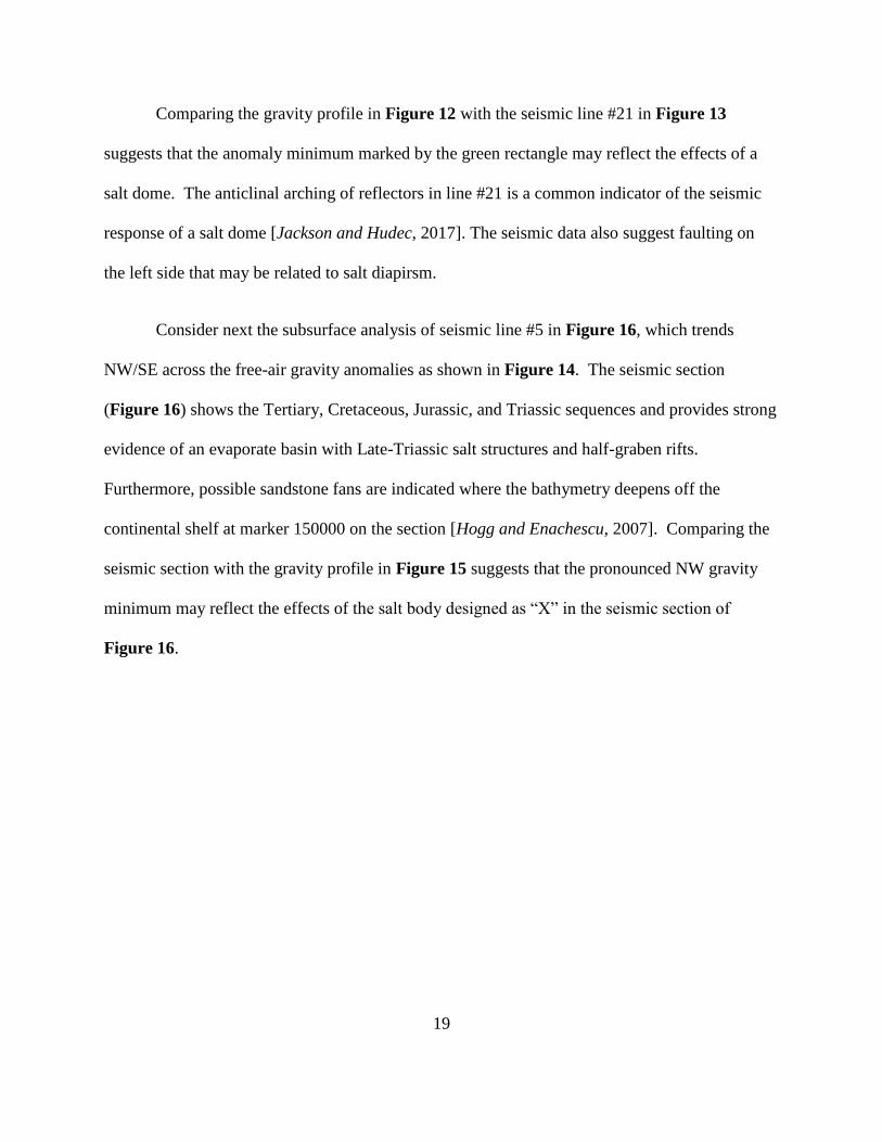
Consider next the subsurface analysis of seismic line #5 in Figure 16, which trends

NW/SE across the free-air gravity anomalies as shown in Figure 14. The seismic section

(Figure 16) shows the Tertiary, Cretaceous, Jurassic, and Triassic sequences and provides strong

evidence of an evaporate basin with Late-Triassic salt structures and half-graben rifts.

Furthermore, possible sandstone fans are indicated where the bathymetry deepens off the

continental shelf at marker 150000 on the section [Hogg and Enachescu, 2007]. Comparing the

seismic section with the gravity profile in Figure 15 suggests that the pronounced NW gravity

minimum may reflect the effects of the salt body designed as “X” in the seismic section of

Figure 16.

20

Figure 14. Seismic reflection line # 5 superimposed on the region’s free-air gravity anomalies.

21

Figure 15. Gravity profile along seismic line #5 running from SE (left) to NW (right).

Figure 16. Seismic reflection line #5 running from NW (left) to SE (right) reveals properties

of an evaporate basin with Late-Triassic salt bodies (e.g., X) and half-graben rifts.

22

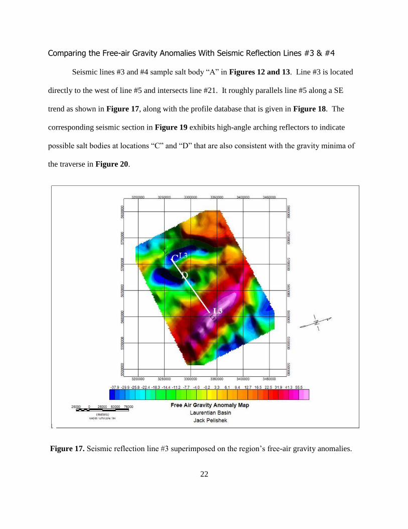
Comparing the Free-air Gravity Anomalies With Seismic Reflection Lines #3 & #4 Seismic lines #3 and #4 sample salt body “A” in Figures 12 and 13. Line #3 is located

directly to the west of line #5 and intersects line #21. It roughly parallels line #5 along a SE

trend as shown in Figure 17, along with the profile database that is given in Figure 18. The

corresponding seismic section in Figure 19 exhibits high-angle arching reflectors to indicate

possible salt bodies at locations “C” and “D” that are also consistent with the gravity minima of

the traverse in Figure 20.

Figure 17. Seismic reflection line #3 superimposed on the region’s free-air gravity anomalies.

23

Figure 9. Seismic Line 3.

Figure 18. Profile of free-air gravity anomalies along seismic reflection line #3

running from NW (top) to SE (bottom). The values range from 0 km to 41 km

within the green rectangle on the gravity traverse (Figure 20).

24

Figure 19. Seismic reflection line #3 running from NW (left) to SE (right) interpreted for the

location of salt bodies “C” and D”.

Figure 20. Gravity profile along seismic reflection line #3 running from NW (left) to

SE (right). The green rectangle outlines the anomaly minima that most likely reflect

the effects of salt structures “C” and D”.

25

Lastly, the seismic reflection line #4 is shown in Figure 22, where the salt body “E” has

been interpreted from the high arching reflectors. The seismic line is plotted on the region’s

free-air gravity anomalies in Figure 21 with the gravity profile displayed in Figure 23 from the

SE to NW. The gravity minimum within the green rectangle of Figure 23 is consistent with the

density deficient effects of the inferred “E” salt body.

Figure 21. Seismic reflection line #4 superimposed on the region’s free-air gravity

anomalies.

26

Figure 22. Seismic Line #4. Note: this line runs in reverse from

left to right

Figure 22. Seismic Line #4 running from SE (left) to NW (right) interpreted

for the location of salt body “E”.

Figure 23. Gravity profile along seismic reflection line #4 running from NW

(left) to SE (right). The green rectangle outlines the anomaly minima that most

likely reflects the effects of salt structure “E”.

27

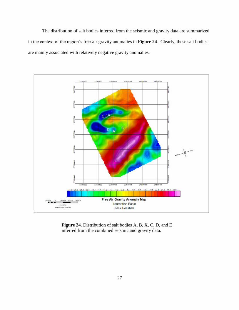
The distribution of salt bodies inferred from the seismic and gravity data are summarized

in the context of the region’s free-air gravity anomalies in Figure 24. Clearly, these salt bodies

are mainly associated with relatively negative gravity anomalies.

Figure 24. Distribution of salt bodies A, B, X, C, D, and E

inferred from the combined seismic and gravity data.

28

DISCUSSION

Understanding the Gravity Response of Salt

Gravity data are very useful in imaging salt domes because of the large negative density

contrast that arises between a salt body and the surrounding strata [Chandler and Burns, 2015].

In particular, a negative density contrast of -85 kg/𝑚3 results from subtracting the Laurentian

Basin’s sediment density of 2,250 kg/𝑚3 from the salt’s density of 2,165 kg/𝑚3. Gravity

anomalies are defined as small deviations of gravity caused by lateral density variations in the

subsurface [Filcher et al., 2016]. Furthermore, salt density remains constant at any depth

[Ruder, 2010].

Accordingly, salt represents a viable source for the negative horse-shaped gravity

anomalies of the region. In general, interpretations of gravity and seismic data by themselves are

non-unique. However, as shown by these datasets in combination can greatly limit the

ambiguities of interpretation.

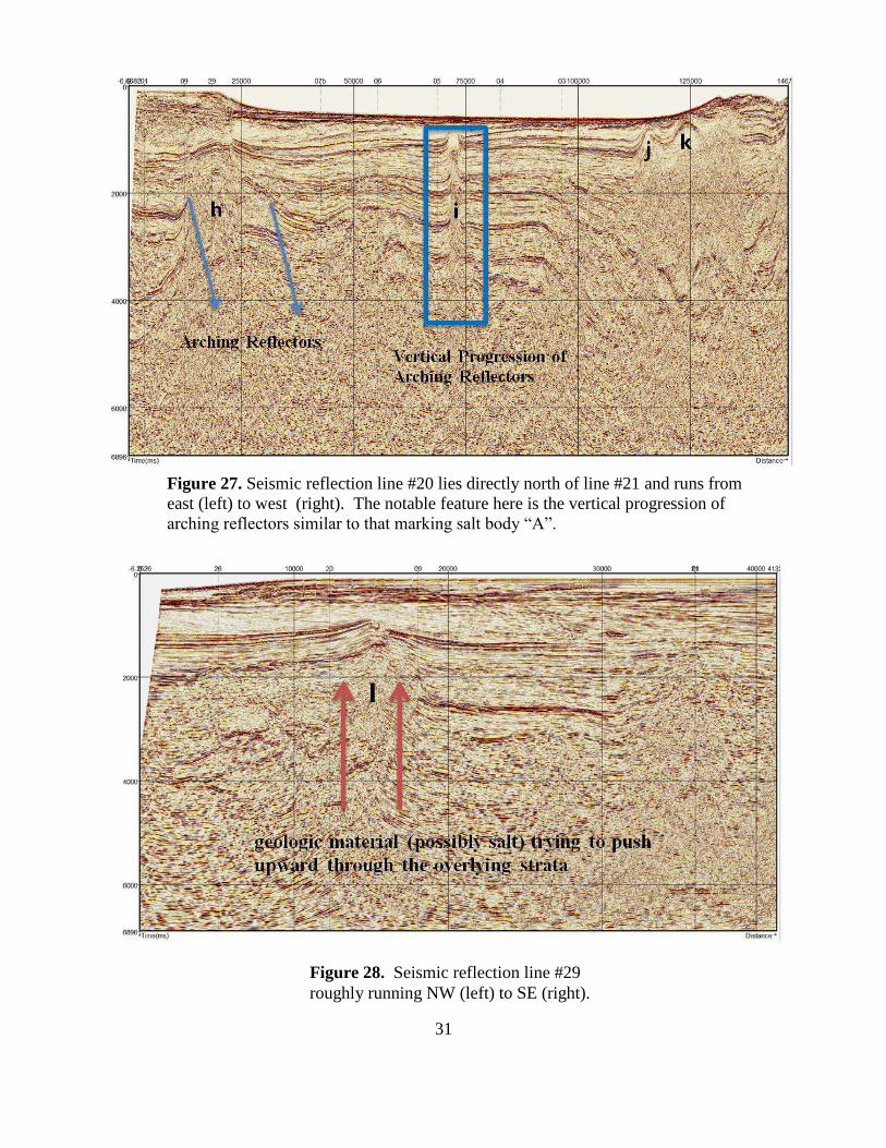
Additional Salt Bodies on Seismic Reflection Lines #1, #6, #20, & #29

Additional salt bodies are suggested by arching reflectors on the seismic reflection lines

#1 (Figure 25), #6 (Figure 26), #20 (Figure 27), and #29 (Figure 28). However, these salt

bodies lack prominent correlative gravity minima, and thus these interpretations are not marked

by the confidence level of the previously interpreted salt bodies. Accordingly, lowercase letters

are used to mark the salt bodies from these lower confidence interpretations. For example, on

the seismic section #1 (Figure 25), the salt body “f” is marked by a narrow and long vertical

extension of upward arching reflectors. The sharp high angle of the reflector provides strong

29

evidence for the existence of salt. On the seismic section #6 (Figure 26), 2 particularly

prominent salt bodies “g” and “m” are inferred from the very high arching reflectors.

Figure 25. Seismic reflection line #1 running roughly from NW (left) to SE (right)

through the middle of the study area as shown in Figure 29. This line is located east of

line #5 and is roughly parallel to line #5 and also intersects line #21. Salt diapirism is also

evident, as well as the shelf breaks at marker 150000.

30

In the seismic section #20 (Figure 27), salt bodies “j”, “k”, and “h” exhibit high arching

reflectors, and “i” resembles the multiple vertical sections of arching reflectors similar to those

of the salt bodies “A” and “f”. Seismic line #29 (Figure 28) is the easternmost section

examined, which reveals a possible salt body at location “l”. This is the least confident marked

salt body, but the upward arching reflectors on this profile suggest an upward migrating salt

body.

Figure 26. Seismic reflection line #6 running roughly from SE (left) to NW (right) through the

western half of the study area as shown in Figure 29. This line is located to the east of line #5

and is roughly parallel to line #5. It also intersects line #21. Between line #20 and marker

150000, the reflectors display dramatic arching typical of a salt dome on a seismic profile.

31

Figure 28. Seismic reflection line #29

roughly running NW (left) to SE (right).

Figure 27. Seismic reflection line #20 lies directly north of line #21 and runs from

east (left) to west (right). The notable feature here is the vertical progression of

arching reflectors similar to that marking salt body “A”.

32

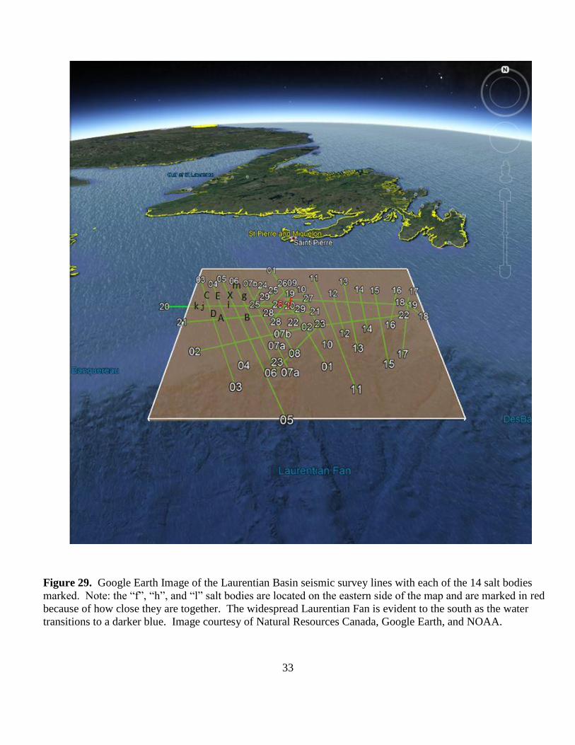
Plotting of Salt Bodies on Google Earth

To help visualize the distribution of the salt in the Laurentian Basin, the seismic lines and

fourteen salt dome locations were projected onto the Google Earth image of Figure 29. Six of

the bodies were designated with high confidence (upper case) and eight of the bodies were

assigned medium confidence (lower case). The inferred salt bodies A, B, X, C, D, e, f, g, h, i, j,

and l are also superimposed to the gravity anomaly map in Figure 30. Eleven of the fourteen salt

bodies are organized together in the northwest part of the seismic survey, which is where the

high and negative anomalies are present. The distribution of salt bodies in the northwest corner

suggests that this area is a potential target for exploration. Although much of the basin has yet to

be explored, the Laurentian Basin presents promising opportunities to oil and gas companies.

33

Figure 29. Google Earth Image of the Laurentian Basin seismic survey lines with each of the 14 salt bodies

marked. Note: the “f”, “h”, and “l” salt bodies are located on the eastern side of the map and are marked in red

because of how close they are together. The widespread Laurentian Fan is evident to the south as the water

transitions to a darker blue. Image courtesy of Natural Resources Canada, Google Earth, and NOAA.

34

Figure 30. The distribution of inferred salt bodies A, B, X, C, D, E, f, g, h, i, j, k, and

l superimposed on the region’s free-air gravity anomalies.

35

The Laurentian Fan

The effects of the Laurentian Fan on the Atlantic Ocean bathymetry and gravity response

were not addressed until the feature was discovered on Google Earth and a gravity pattern

appeared. The fan is described in the literature as a 0.5 to 2 km thick Quaternary fan overlying

Tertiary and Mesozoic sediments [Piper et al., 1983]. Seismic line #5 reveals the best example

of the transition into the Laurentian Fan. This line runs in a southeast direction and is 131.15

miles in length. Likewise, 93.26 miles are covered until the line crosses the shelf and continues

within the shelf for another 37.89 miles.

Looking at seismic line #5 from left to right (Figure 31), at salt dome “X” it makes sense

to observe arching reflectors because they lie in the middle of the dark blue anomaly region. In

comparison, there are also steep and arching reflectors that typically signify a classic salt

structure at the right margin. However, these Cretaceous and Jurassic units are located in the

Laurentian Shelf and are overlain by a prominent positive elliptical NE/SW trending gravity

anomaly maximum of +55.5 mGal. The black curve in Figure 32 marks this continental edge

anomaly [Hinze et al., 2013], where the shelf begins and sheds higher density Mesozoic

sediments to the south.

36

Figure 31. Seismic reflection line #5 annotated to emphasize the drop in bathymetry

into the Laurentian Fan, which displays large and positive gravity anomaly values.

37

Figure 32. Free-air gravity anomaly map showing the approximate continental edge

of the Laurentian Fan. The large and positive gravity anomaly is the edge effect of a

sharply raised mantle at the shelf’s margin.

38

CONCLUSIONS

Comparing the gravity responses for seismic reflection lines #21, #5, #3, and #4

identified likely areas containing crustal salt bodies. The best example was the seismic up-

arching and negative gravity signal correlations that inferred the salt body “A” in the seismic

section #21. This approach was used to infer the distribution of some fourteen salt bodies that, in

turn, were plotted on a Google Earth image to help visualize the hydrocarbon potential of the

Laurentian Basin. Clearly, combining seismic and gravity data is very useful for enhancing the

geological interpretation of the basins, evaluating their hydrocarbon potential, and pinpointing

the distribution of salt domes within the subsurface.

39

RECOMMENDATIONS FOR FUTURE WORK

Future research should extend this work to other basins in the world (e.g. Gulf of Mexico,

offshore Brazil, the North Sea, etc.). This work also might be useful for investigating the mud

diapir versus salt diapir debate in the marine shelf area of North Carolina.

40

REFERENCES CITED

Adam, J., and Krézsek, C., 2012, Basin-scale salt tectonic processes of the Laurentian Basin,

Eastern Canada: insights from integrated regional 2D seismic interpretation and 4D

physical experiments: Geological Society, London, Special Publications, v. 363, p.331-

360.

Asgharzadeh, M., Hashemi, H. and von Frese, R., 2017, Comprehensive Gravity Modeling of the

Vertical Cylindrical Prism by Gauss-Legendre Quadrature Integration: Geophysical

Journal International, v. 212, p.591–611, https://doi.org/10.1093/gji/ggx413.

Canada-Newfoundland and Labrador Offshore Petroleum Board, 2012, Offshore Opportunity,

Call for Bids NL12-01, Laurentian Basin, Offshore Newfoundland:

http://www.nr.gov.nl.ca/nr/invest/cfb1201executivesummary.pdf (accessed June 2017).

Chandler, G., and Burns, C., 2015, Giving Seismic an Uplift with Gravity and Magnetics:

http://www.earthexplorer.com/2015/Giving_seismic_an_uplift_with_gravity_and_magne

tics.asp (accessed June 2017).

Fagan, A.J., and Enachescu, M., 2007, The Laurentian Basin Revisited, in Proceedings,

CSPG/CSPE GeoConvention, Calgary, Canada, May 2007.

Filcher, C., Landro, M., and Amundsen, L., 2016, Gravity for Hydrocarbon Exploration:

GEOExPro Magazine, v. 13, p.60-63.

Hinze, W., von Frese, R., & Saad, A., (2013). Gravity and Magnetic Exploration: Principles,

Practices, and Applications. Cambridge: Cambridge University Press.

doi:10.1017/CBO9780511843129.

41

Hogg, J., and Enachescu, M., 2007, Exploration Potential of the Deepwater Petroleum Systems

of Newfoundland and Labrador Margins, in Proceedings, Offshore Technology

Conference, Houston, Texas, May 2007.

Jackson, M., and Hudec, M., (2017). Salt Tectonics: Principles and Practice. Cambridge:

Cambridge University Press. doi:10.1017/9781139003988.

Piper, D.J.W., Stow, D.A.V. & Normark, W.R., The Laurentian Fan: Sohm abyssal plain: Geo-

Marine Letters (1983) 3: 141. https://doi.org/10.1007/BF02462459.

Ruder, M., 2010, When Seismic Isn’t Enough:

http://www.earthexplorer.com/news/When_seismic_isnt_enough.asp (accessed June

2017).

Saad, A. H., 1993, Interactive Integrated Interpretation of Gravity, Magnetic, and Seismic Data:

Tools and Examples, in Proceedings, Offshore Technology Conference, Houston, Texas,

May 1993.