Sectoral Linkages and Industrial Efficiency: A

Dilemma or a Requisition in Identifying Development

Priorities?

Giannis Karagiannis

(Dept. of International and European Economic and Political Studies, University of

Macedonia, Greece)

Vangelis Tzouvelekas

(Dept. of Economics, University of Crete, Greece)

June 2003

Please direct correspondence to:

Vangelis Tzouvelekas

Dept. of Economics, University of Crete University Campus, 741 00 Rethymno, Crete, GREECE. Phone: +30-28310-77417; Fax: +30-28310-77406; e-mail: vangelis@econ.soc.uoc.gr

Sectoral Linkages and Industrial Efficiency: A Dilemma or a

Requisition in Identifying Development Priorities?

Abstract

This paper attempts to provide an empirical evaluation of the potential relationship

between sectoral linkages and technical efficiency using the 1996 US input-output

tables. Sectoral input-oriented technical efficiency is obtained by the econometric

estimation of a stochastic input-distance function based on Battese and Coelli (1995)

model formulation. On the other hand, sectoral backward and forward linkage

coefficients were computed using the non-complete hypothetical extraction method

suggested by Dietzenbacher and Van der Linden (1997). The empirical results

suggest that there is a negative relationship between sectoral efficiency and linkage

coefficients, while on the other hand efficient sectors tend to purchase their

intermediate inputs from efficient sectors and vice versa.

1. Introduction

In forming economic development policies the assessment of sectoral economic

performance and production interdependence are both very important issues. While,

sectoral interdependence is one of the most important source of economic expansion

in a competitive economy, efficiency is the most important control parameter for

assessing the utilization of inputs in the production process. A large and strongly

interdependent sector may be seen as a good candidate for the economic development

of a particular country or region. The expansion of this sector will have a significant

impact, increasing output, income or employment domestically.

However, and equally important, a sector that operates more efficiently (i.e.

producing as much output as the inputs at its disposal permit under the current state of

technology) compared to the same sector in other countries or regions could be a

better candidate for long term growth and development. That’s because efficiency is

one of the main factors determining the overall competitiveness of a sector. The

higher the degree of efficiency, the lower will be the unit cost of production and as a

result, industries will be able to supply their products at lower prices. Consequently,

more efficient industries would have better chances of surviving and prospering in the

- 1 -

future than less efficient ones. Furthermore, improvements in sectoral efficiency can

increase productivity and thus output growth within the national or regional economy,

thus providing a more cost-effective way for stimulating internal economic growth.

In the short-run, an economic sector may be large enough to attract policy

attention but if it is not operating efficiently compared to the same sector in other

nations or regions, sooner or later it will become less competitive and begin to

diminish from external competitive pressures. It is evident therefore, that it is

important to know how much a given sector can stimulate economic growth within

the economy without resource waste, thereby improving its competitive status. In a

long-term competitive environment the overall efficiency and thus productivity of a

national or regional economy determines the general well-being of its people

(Krugman, 1991).

Traditionally, input-output analysis and the subsequent measurement of linkage

coefficients has been used excessively for the identification of key economic sectors

in both national and regional economies. Since the pioneering work of Rasmussen

(1956), Chenery and Watanabe (1958) and Hirschman (1958), a number of studies

employing input-output techniques have relied on linkage analysis to describe the

interdependent relationships between economic sectors and to assist in the

formulation of economic development strategies. The economic rationale behind the

empirical significance of linkage analysis is rather simple: the expansion of sectors

with strong linkages and thus production interdependencies within the economy is

likely to promote overall economic development.

Through the years the methodological framework has been improved and

expanded in several ways, and many different analytical methods have been proposed

for the measurement of interindustry linkage coefficients (i.e. Jones, 1976; Cella,

1984; Heimler, 1991; Sonis et al., 1995; Dietzenbacher and Van der Linden, 1997).

Although it seems that the problem of the appropriate linkage indicator has been

resolved, there still remains an important practical question: would the expansion of

the “key” sectors identified by means of linkage coefficients would indeed promote

economic development?

The aim of this paper is to explore this unknown relationship between sectoral

interdependence and technical efficiency. The empirical analysis is based on the 1996

US input-output tables published by the Bureau of Economic Analysis. Both

backward and forward linkage coefficients were computed using the approach

- 2 -

suggested recently by Dietzenbacher and Van der Linden (1997), which is an adapted

form of Strassert’s (1968) hypothetical extraction method. Measurement of sectoral

technical efficiency is based on Shephard’s (1953) input-distance function which can

easily accommodate multi-output technologies under the assumption of weak

disposability. Finally, the stochastic frontier is modeled according to Battese and

Coelli’s (1995) inefficiency effects model.

The rest of this paper is organized as follows: the methodological framework for

the estimation of backward and forward linkage coefficients using Dietzenbacher and

Van der Linden’s (1997) non-complete hypothetical extraction method is presented in

the next section. The use of Shephard’s input-distance function in stochastic frontier

modelling and the associated measurement of technical efficiency is discussed in the

third section. The empirical model and data sources are presented in the fourth

section. A discussion of empirical findings and a comparison of sectoral technical

efficiency and linkage coefficients are given in the fifth section. Concluding remarks

follow in the last section.

2. Non-Complete Hypothetical Extraction Method

Consider the usual demand and supply-driven1 Leontief input-output systems:

( ) YAXYXXZX +=+= −1 (1a)

and ( ) VBXVZXXX ′+′=′+′=′ −1 (1b)

where X is the vector of sectoral gross output, Z is the transactions matrix, Y is the

vector of sectoral final demand, V is the vector of sectoral final payments and 1−X is

a diagonal matrix of sectoral gross output. Solving the above systems for the vector

of sectoral output X we get:

(2a) [ ] YAIX 1−−=

[ ] 1−−′=′ BIVXand

(2b)

The basic idea of Strassert’s (1968) original approach hinges on the hypothetical

extraction of one sector from the economy and then the examination of the impact of

- 3 -

this hypothetical extraction on other sectors of the economy. Under the usual

assumption of the input-output system, the reduced output vector is less than the

original output vector X. Then the sum of the differential between the output vector X

excluding the k

( )kX~

( )kX~

⎥⎦⎤

⎢⎣⎡+⎥

⎦

⎤⎢⎣

⎡⎥⎦⎤

⎢⎣⎡=⎥

⎦

⎤⎢⎣

⎡

m

a

m

a

mm

am

m

aYY

X~X~

AA

X~X~

00

aX

th element and provide a measure of the total (both backward and

forward) linkage effect of the extracted sector k on total output.

As noted by several authors, the hypothetical extraction method as suggested by

Strassert (1968) has two important shortcomings: first, it fails to distinguish between

backward and forward linkages, and second, the complete extraction of an entire

sector from the system seems to be rather excessive (i.e. Meller and Marfán, 1981;

Cella, 1984; Clements, 1990).

Recognizing the above deficiencies, Dietzenbacher and Van der Linden (1997)

improved the methodological framework suggesting a non-complete extraction

method.2 Their approach is based on the assumption that backward linkages should

reflect a sector’s interdependence on inputs that are produced within the economy.

Therefore, only these intermediate inputs should be hypothetically eliminated in order

to measure the backward linkages.

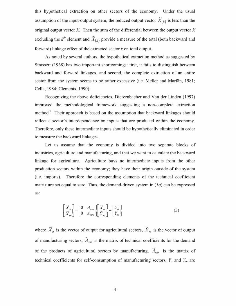
Let us assume that the economy is divided into two separate blocks of

industries, agriculture and manufacturing, and that we want to calculate the backward

linkage for agriculture. Agriculture buys no intermediate inputs from the other

production sectors within the economy; they have their origin outside of the system

(i.e. imports). Therefore the corresponding elements of the technical coefficient

matrix are set equal to zero. Thus, the demand-driven system in (1a) can be expressed

as:

(3)

where ~ is the vector of output for agricultural sectors, mX~ is the vector of output

of manufacturing sectors, amA~ is the matrix of technical coefficients for the demand

of the products of agricultural sectors by manufacturing, is the matrix of

technical coefficients for self-consumption of manufacturing sectors, Y

mmA~

a and Ym are

- 4 -

the final demand vectors of the agricultural and manufacturing sectors, respectively.

Solving the above system for iX~ (i=a, m) we obtain:

( )

( ) ⎥⎦⎤

⎢⎣⎡⎥⎦

⎤⎢⎣

⎡ −=⎥⎦

⎤⎢⎣

⎡−

−

m

a

mm

mm

m

aYY

AAAI

X~X

−am

II~

1

1

0

⎥⎦

⎤⎢⎣

⎡−−′=

mm

aaDa X~X

X~XeABL

[ ]

(4)

The absolute backward linkage is defined as the difference between actual total

output of the economy and that after the extraction of the agricultural sectors. The

latter is less than the former due to the fact that agricultural sectors no longer depend

on manufacturing with regard to their input requirements. This output decrease

reflects the dependence of the agricultural sector on manufacturing, as well as on

itself.3

(5a)

( )

( )[] mmm

mmamama

YG

GAIDYDA +−+

=mmG

ammamm

mmDa

DAAGe

GeIDABL′

′+−= (5b)

where , ( ) 1−− mmAI ( ) 1−−−= mammamaa AGAAID and e is a vector of ones.

The magnitude of the above absolute backward linkage is determined by two factors:

first the relative size of the sector, and second, its dependence per unit of output (its

output multiplier). Since the primal concern is the sectoral interdependence,

Dietzenbacher and Van der Linden (1997) suggest normalizing the above value by

dividing the absolute figures by the value of sectoral output. This results in the

backward dependence of agricultural sectors on manufacturing as:

a

DaD

a XABL

BL = (6)

In a similar manner to backward linkages, forward linkage indicators can be

obtained using the supply-driven Leontief input-output system (Dietzenbacher and

Van der Linden, 1997).4 These backward (forward) linkages actually examine the

extent of the impact derived from the hypothetical extraction of a sector on total

output when final demand (or primary inputs) increases in all sectors in the economy.

- 5 -

This includes the effect of all other sectors on total output through the feedback in

connection with the inputs (or sales) of the hypothetical extracted sector (Andreosso-

O’Callaghan and Yue, 2000).

3. The Stochastic Input-Distance Function and the Measurement of Technical

Efficiency

Let us assume that the industrial sectors use a non-negative vector of inputs

to produce a non-negative vector of outputs . This defines a

production possibility set

kRx +∈ mRy +∈

( ){ }y produce can x :Rx,y nm++∈=T . Then for all x we can

define an input requirement set such that ( ) ( ){ }TRxyL n∈= +

( )

xy, : ∈ describing the

input vectors that are feasible for producing output vector y. In terms of inputs

correspondence the input-distance function is defined by (Russell,

1998):

+→ RN:D I

( )}yL∈ { x:maxx,yD I >= λλ 0

( )

(7)

( ) ( ) ( ){ }0λ someorf yN nnm >= +

( )yLx∈

( )

LλxyL0:Rxy, ∈∧∉∈ +where . The input-

distance function defined above provides a radial measure of the distance from an

input bundle to the corresponding isoquant, the lower bound of the input requirement

set. Thus it provides a direct link between the functional characterization of the

production technology and radial efficiency measurement. If, for example,

but it does not belong to the corresponding isoquant, so that the input vector x can

produce y given the technology T, the same output vector could be produced with less

of all inputs if the production unit operated closer to the isoquant. In other words, the

producer in question operates technically inefficiently in producing y in the sense of

Farrell’s (1957) definition. Hence, a radial measure of input-oriented technical

efficiency can be given by the reciprocal of the input-distance function as (Färe and

Lovell, 1978):

( ]101 ,x,yD

TE II ∈= (8)

- 6 -

Which reveals the maximum radial contraction of the input vector such that the

production of the output vector is still feasible. Quantitative measures of input-

oriented technical efficiency can be obtained by econometrically estimating an input-

distance function. This is feasible with only input and output quantity data, and the

use of a single-equation estimation procedure is consistent with the fact that the input-

distance function is agnostic with respect to the economic motivation of the decision-

makers (Grosskopf et al., 1995). More importantly, flexible functional forms can be

used that do not impose any a priori restrictions on the structure of production.

The translog function is such a flexible functional form that it may be used to

approximate the underlying input-distance function. It is given as (see Coelli and

Perelman, 1999; Grosskopf et al., 1995; Bosco, 1996):

lm

M

m

M

lmlk

K

kkm

M

mm

I ylnylnxlnyln)x,y(Dln ∑∑∑∑= ===

+++=1 111

0 21 αβαα

kmm k

mkjkk j

kj xlnylnxlnxln ∑∑∑∑= == =

++1 11 12

δβ M KK K1

11

=∑=

K

kkβ 0

11== ∑

==

M

mmk

K

kkj δβ lmml

(9)

The required regularity conditions include homogeneity of degree one in inputs

and symmetry. These imply the following restrictions on the parameters of (9):

, ∑ , αα = jkkj ββ = (10) and

The homogeneity restrictions may also be imposed by dividing the left-hand

side and all input quantities in the right-hand side of (9) by the quantity of that input

used as numeraire.

Given the imposition of linear homogeneity, to obtain an estimable form of the

input-distance function, rewrite (9) as ( )x,yDln)(fxln Ik −⋅=−

)(f ⋅

( )x,yD I

, where k is the

numeraire input and is the right-hand side of (9). Since there are no

observations for ln and given that ( ) 0≤x,yDln I we can make the

following replacement: , where u( ) iux,y −=IDln i is a one-side, non-negative, error

term representing the stochastic shortfall of the ith producer’s output from its

production frontier, due to the existence of input-oriented technical inefficiency

- 7 -

(Coelli and Perelman, 1999). Then, the stochastic input-distance function model may

be written as:

iiki vu)(fxln +−⋅=−

i

H

hhihoi zu ωρρ ++= ∑

=1

2ωσ

( )∑+−≥ hihi zρρω 0

+= hihi zρρµ 02ωσ

(11)

where vi depicts a symmetric and normally distributed error term (i.e., statistical

noise), which represents those factors that cannot be controlled by producers, left-out

explanatory variables and measurement errors in the dependent variable. It is also

assumed that vi and ui are independently distributed from each other.

Since our purpose in this paper is to explore the possible relationship between

industrial linkages and technical efficiency we can replace the technical inefficiency

effects, ui, in (11) by a linear function of backward and forward linkages coefficients

following the Battese and Coelli (1995) model formulation. Specifically,

(12)

where zhi are sectoral-specific backward and forward linkage coefficients; ρ0 and ρh

are parameters to be estimated; and ωi is a random variable with zero mean and

variance , defined by the truncation of the normal distribution such that

. The above specification (12) implies that the means,

, of the u∑ i are different for different sectors but the variances, ,

are assumed to be the same.

4. Data and Empirical Model

The comparative evaluation of sectoral linkage coefficients and technical

efficiency was applied to the 1996 US input-output tables published by the Bureau of

Economic Analysis (BEA) of the USDC. These tables are based on an update of the

1992 benchmark input-output accounts and they reflect the recent comprehensive

revision of the national income and product accounts. The input-output accounts

were transformed to an industry-by-industry framework (94 industries) assuming an

industry-based technology prior to the estimation of linkage coefficients and sectoral

technical efficiency (Miller and Blair, 1985, pp. 159-171; Jansen and ten Raa, 1990).

- 8 -

The stochastic input-distance function includes two outputs and four inputs. The

output measures are: (1) the total domestic sectoral output measured as the sum of

production sold to other sectors within the economy as intermediate goods, to final

consumption, and to fixed capital formation; (2) the total sectoral exports. The

decomposition by type of purchases into domestic and foreign markets is based on the

methodological framework developed by Diewert and Morrison (1988), Lawrence

(1990) and Nadiri and Son (1999).

The input measures are: (1) the total labor cost including wages and salaries and

all kinds of benefits paid by state industries; (2) the total sectoral intermediate

consumption purchased domestically; (3) the total value of sectoral capital stock; (4)

the total sectoral imports.5 In the inefficiency effects model, we have included the

corresponding backward and forward linkage coefficients obtained from

Dietzenbacher and Van der Linden’s (1997) non-complete hypothetical extraction

method.

5. Empirical Results

The maximum likelihood parameter estimates of the translog input-distance

frontier function along with their corresponding standard errors are presented in Table

1. The translog input-distance frontier function is found at the approximation point to

be non-increasing in outputs and non-decreasing in inputs. Also, at the point of

approximation, the Hessian matrix of the first- and second-order partial derivatives is

found to be negative definite with respect to inputs and positive definite with respect

to outputs. These indicate the concavity and convexity of the underlying input-

distance function for inputs and outputs, respectively. Finally, the logarithm of the

likelihood function indicates a satisfactory fit for the particular functional

specification.

Several hypotheses concerning model representation were examined.6 First, the

average input-distance function does not adequately represent the structure of

technology. The null hypotheses that 00 === hρργ and 0=γ are rejected at the

5% level of significance, indicating that the technical inefficiency effects are in fact

stochastic (this is also depicted by the statistical significance of the γ-parameter).7

Thus, a significant part of output variability among industries is explained by the

existing differences in the degree of input-oriented technical inefficiency.

- 9 -

In addition, our specification of the frontier model cannot be reduced to the

models of either Aigner et al. (1977) or Stevenson (1980), as the null hypotheses of

00 == h ρρ 0=h ρ and , respectively, are rejected at the 5% level of

significance. As a result, the explanatory variables included in the inefficiency effect

models have non-zero coefficients and contribute significantly to the explanation of

technical efficiency differences among US input-output sectors.

h∀

The frequency distribution of input-oriented technical efficiency ratings among

US industries is presented in Table 2. The estimated mean technical efficiency was

found to be 70.33%. Since input-oriented technical efficiency has a direct cost

interpretation, this figure means that on average, a 29.67% decrease in total cost of

production could be achieved, without altering the total volume of output, production

technology and input usage. In other words it is possible for the US economy to

become more technically efficient and to maintain the same level of sectoral output by

reducing by almost 30% labour cost, intermediate consumption, capital equipment

and imports.

The variation of technical efficiency ratings is considerable (the standard

deviation is 17.7%). Specifically, sectoral technical efficiency ranges between a

minimum of 40.92% and a maximum of 98.71%. It is important to note that only

36% of the industries achieved technical efficiency levels above 80%, while on the

other hand there are 17 industries with technical efficiency levels below 50%. For

these sectors considerable gains can be attained in their overall competitiveness by

improving their resource use.

Among the sectors with the highest technical efficiency levels are: Owner-

Occupied Dwellings (98.71%), Wholesale Trade (97.05%), Federal Government

Enterprises (97.05%), Retail Trade (96.88%) and Insurance (95.78%). Conversely the

sectors with the lowest technical efficiency levels include: Paints and Allied Products

(40.92%), Primary Non-Ferrous Metals Manufacturing (41.73%), Metallic Ores

Mining (41.85%), Agricultural Fertilizers and Chemicals (42.32%) and Engines and

Turbines (43.10%).

Backward and forward linkage coefficients computed using the Dietzenbacher

and Van der Linden (1997) non-complete hypothetical extraction method are also

reported in Table 2 in the form of frequency distribution. The average of the sectors’

backward and forward linkage values are more or less the same, 0.784 and 0.778,

- 10 -

respectively. The empirical results reveal a weak relationship between backward and

forward linkages. However, this relationship does not hold in general since backward

linkages are measured with respect to purchasing sectors, whereas forward linkages

are measured with respect to selling sectors.

For the majority of the input-output sectors the relevant backward linkage

coefficient is below unity. There are only 17 sectors with a backward linkage

coefficient value above one. The highest values are observed for the Metal

Containers and Livestock sectors, 1.537 and 1.376, respectively. These values mean

that if intermediate purchases of these sectors were hypothetically removed, the total

output of the US economy would fall by 1.537 and 1.376 times this particular sector’s

actual output.

The first five sectors with the highest backward linkage coefficient value are

Metal Containers (1.537), Livestock and Livestock Products (1.376), Paperboard

Containers and Boxes (1.298), Petroleum Refining and Related Products (1.276) and

Miscellaneous Textile Goods and Floor Coverings (1.220). Conversely among the

sectors with the lowest backward linkage coefficient value are Owner-Occupied

Dwellings (0.218), Real Estate and Royalties (0.399), Federal Government

Enterprises (0.408), Other Business and Professional Services (0.426) and Footwear,

Leather and Leather Products (0.443).

The highest forward linkage coefficient value is 1.865 achieved by Metallic

Ores Mining. Therefore, if the intermediate sales of this particular sector were

hypothetically removed from the system, the total output of the US economy would

fall by 1.865 times the actual output of Metallic Ores Mining. The variation of

forward linkages between sectors is larger than that of backward linkages. The

standard deviations are 0.273 and 0.504 for backward and forward linkages,

respectively. There are 33 sectors with a corresponding forward linkage coefficient

value below 0.500, and 34 sectors with a forward linkage coefficient value above one.

Roughly speaking, sectors for which a large part of their output is destined for

final demand purposes have weak forward linkages, whereas sectors whose output is

primarily used for further production have strong forward linkages. The highest

forward linkages are attained by Metallic Ores Mining (1.865), Non-Metallic

Minerals Mining (1.785), Pipelines, Freight Forwarders and Related Services (1.670),

Federal Government Enterprises (1.657) and Agriculture, Forestry and Fishery

(1.626). On the other hand, the sectors with the lowest forward linkage coefficients

- 11 -

are Furniture and Fixtures (0.103), Retail Trade (0.108), Educational and Social

Services (0.122), New Construction (0.136) and Other Transportation Equipment

(0.138).

Concerning the relationship among backward and forward linkages and

technical efficiency, the corresponding parameter estimates in the inefficiency effects

model were found to be negative and strongly significant, -0.913 and -0.132,

respectively (see Table 1). Furthermore, the Spearman correlation coefficients among

sectoral linkage coefficients and technical efficiency levels verify this negative

relationship (see bottom line of Table 2). This means that high sectoral technical

efficiency levels are generally associated with low backward and forward linkage

values. In other words, sectors with a high potential to stimulate output growth within

the US economy, are not using an optimal allocation of their existing resources.

Strengthening further the above finding Table 3 presents the first fifteen I-O

sectors with the highest and lowest technical efficiency along with their

corresponding backward and forward linkage coefficient values. As is clearly

perceived from this table, apart from some notable exceptions, the general tendency is

towards this negative relationship. Metal Containers, the sector with the highest

backward linkage value, and Metallic Ores Mining, the sector with the highest

forward linkage value achieve technical efficiency levels of only 46.67% and 41.58%,

respectively.

On the other hand, Owner-Occupied Dwellings, the sector with the highest

technical efficiency score, has backward and a forward linkage values of only 0.218

and 0.205 respectively. Contrarily, Paints and Allied Products, the sector with the

lowest technical efficiency score, has backward and forward linkage values of 1.170

and 1.293, respectively.

Among the 30 sectors presented in Table 3, only seven -Eating and Drinking

Places, New Construction, Crude Petroleum and Gas, Federal Government

Enterprises, Other Business and Professional Services, Legal, Maintenance and

Repair Construction and Materials Handling Machinery and Equipment- exhibit a

relative correspondence between their technical efficiency and backward or forward

linkage coefficients. The general tendency, however, is towards this negative

relationship.

This finding, though not general, is rather important and should be taken into

consideration in identifying sectoral development priorities for the US economy. For

- 12 -

instance, according to backward and forward linkage coefficients, the Metal

Containers sector seems to be a good candidate to promote overall economic

development in the US economy as it exhibits strong interdependence with the rest of

the economic sectors. However, the expansion of this particular sector would cause

significant resource waste for the entire economy, while on the other hand the long-

run viability of the anticipated economic benefits would not be as expected. The

Metal Containers sector is operating far from its realized production frontier,

achieving a technical efficiency level of only 46.67%.

In the next step we attempt to investigate whether or not efficient (inefficient)

sectors purchase their inputs primarily from efficient (inefficient) sectors. Table 4

presents the amounts of intersectoral purchases per dollar of intermediate

consumption expressed in percentages by every sector in the US economy. Columns

present buying sectors and rows present producing sectors in a frequency distribution

form according to their technical efficiency levels. As is clearly visible from this

table, sectors with high technical efficiency levels purchase their inputs primarily

from other highly technically efficient sectors. Specifically, sectors with a technical

efficiency level above 90% purchase 74.1% of their intermediate consumption from

sectors with a technical efficiency score above 80%. The situation is also the same

for the sectors with technical efficiency within the 90-80 interval.

On the other hand, sectors with low technical efficiency levels tend to purchase

the necessary inputs for their production from sectors with low technical efficiency

levels. Sectors with technical efficiency ratings within the 50-40 interval purchase

40.7% of their resources from sectors with technical efficiency levels within the 60-40

interval. Although this share of intermediate purchases is not so high as it is for the

technically efficient sectors, it is still significant, revealing a relative correspondence

of the technical efficiency levels between the buying and selling sectors. On the

average, 47.7% (27.9%) of total intersectoral purchases stem from sectors with

technical efficiency levels above 80% (below 60%).

Exploring further the above finding, Table 5 presents the intersectoral purchases

of the ten most and least technically efficient sectors by every other sector in the US

economy. As is evident from this table, efficient sectors tend to purchase their

intermediate inputs mainly from highly efficient sectors (upper panel of Table 5). For

instance the case of the Owner-Occupied Dwellings sector is more profound as 92.5%

- 13 -

of its total intersectoral purchases originate from sectors with technical efficiency

levels above 90%.

In the Wholesale Trade, Federal Government Enterprises, Retail Trade, Health

Services, Educational and Social Services, New Construction and Other Business and

Professional Services sectors, a large portion of their intermediate purchases stem

from other efficient sectors (above 80%), 64.9%, 57.1%, 70.8%, 79.1%, 83.9%,

45.9% and 57.4%, respectively. It is also noteworthy that these intermediate

purchases originate mainly from other sectors in the economy, with only two

exceptions. For the Insurance and Finance sectors, 50.9% and 36.8% of their

intermediate inputs arise from their own production process.

The ten least technically efficient sectors (lower panel of Table 5) reveal the

same pattern though not so strongly. Specifically, in the Paints and Allied Products,

Primary Non-Ferrous Metal Manufacturing, Metallic Ores Mining, Agricultural

Fertilizers and Chemicals, Engines and Turbines, Materials Handling Machinery and

Equipment, Coal Mining and Miscellaneous Textile Goods sectors a large share of

their intermediate purchases originates from relatively inefficient sectors (below

60%), 32.6%, 38.1%, 40.6%, 43.8%, 54.9%, 48.7%, 44.4% and 65.7%, respectively.

There are, however, two exceptions -the Plastic and Synthetic Materials and

Paperboard and Containers Boxes sectors- whose intermediate inputs stem from

relatively more efficient sectors.

6. Conclusions

In identifying sectoral development priorities the assessment of both sectoral

economic performance and production interdependence are very important issues. A

sector with strong interindustry transactions may be seen as a good candidate to

promote overall economic development. However, if the same sector operates

inefficiently, in the sense that it does not produce as much output as its input usage

allows, the anticipated benefits would not be as great as initially expected.

Along these lines we attempted in this paper to present an empirical evaluation

of the potential relationship between technical efficiency and sectoral linkages using

recent methodological advances both in stochastic frontier modeling and in the

measurement of interindustry linkages. The empirical results reveal a rather strong

negative relationship. Technically efficient sectors tend to exhibit low backward and

- 14 -

forward linkage coefficients and vice versa. This is confirmed from case to case

examination as well as from the corresponding parameter estimates in the inefficiency

effects model and Spearman correlation coefficients.

Strengthening further the above finding, we attempted to investigate whether or

not technically efficient (inefficient) sectors purchase their intermediate inputs from

other technical efficient (inefficient) sectors. The results suggest that indeed the

majority of US sectors with a high technical efficiency level (above 80%) tend to buy

intermediate inputs from other technically efficient sectors. This correspondence,

although not so strong, is also observed for technically inefficient sectors (below

60%). Certainly the attained efficiency score of any given sector depends primarily

on its own performance which, however, reflects the specific demand and supply

situation it faces. However, our results suggest a possible pattern of intermediate

sectoral transactions that should be taken into consideration in forming development

plans.

Our empirical results although case specific can provide useful guidelines for

policy makers in appropriately identifying the development prospects of a given

sector in any regional or national economic system. For example, a technically

efficient sector with a high linkage coefficient could serve as a good candidate for

promoting internal economic development. This would give a competitive advantage

to the specific economic system, contributing at the same time to its internal economic

growth in terms of output, income or employment generation.

- 15 -

References

Aigner, D.J., Lovell, C.A.K. and P. Schmidt (1977). Formulation and Estimation of Stochastic Frontier Production Function Models. Journal of Econometrics 6, 21-37.

Andreosso-O’Callaghan, B and G. Yue (2000). Intersectoral Linkages and Key

Sectors in China 1987-1997: An Application of Input-Output Linkage Analysis. XIII International Conference on Input-Output Techniques, 21-25 August, Macerata, Italy.

Augustinovics, M. (1970). Methods of International and Intertemporal Measures of

Structures, in A.P. Carter and A. Brody (Eds.), Contributions to Input-Output Analysis, Amsterdam: North Holland.

Battese, G.E. and T.J. Coelli (1995). A Model for Technical Inefficiency Effects in a

Stochastic Frontier Production Function for Panel Data, Empirical Economics 20, 325-32.

Bosco, B. (1996). Excess-input Expenditure Estimated by Means of an Input Distance

Function: The Case of Public Railways. Applied Economics 28, 491-97. Cella, G. (1984). The Input-Output Measurement of Interindustry Linkages. Oxford

Bulletin of Economics and Statistics 46, 73-84. Chenery, H.B. and T. Watanabe (1958). International Comparisons of the Structure of

Production. Econometrica 26, 487-521. Clements, B.J. (1990). On the Decomposition and Normalization of Interindustry

Linkages. Economics Letters 33, 337-340. Coelli, T.J. and S. Perelman (1999). A Comparison of Parametric and Non-parametric

Distance Functions: With Application to European Railways. European Journal of Operational Research 117, 326-339.

Dietzenbacher, E. and J. Van der Linden (1997). Sectoral and Spatial Linkages in the

EC Production Structure. Journal of Regional Science 37, 235-257. Diewert, W.E. and C.J. Morrison (1988). Export Supply and Import Demand

Functions: A Production Theory Approach, in R.C. Feenstra (Ed.), Empirical Methods of International Trade, Cambridge: MIT Press, 207-222.

Färe, R. and C.A.K. Lovell (1978). Measuring the Technical Efficiency of Production,

Journal of Economic Theory 19, 150-62. Farrell, M.J. (1957). The Measurement of Productive Efficiency. Journal of Royal

Statistical Society Series A General, 120, 253-281. Ghosh, A. (1958). Input-Output Approach in an Allocation System. Economica 25,

58-64.

- 16 -

Grosskopf, S., Hayes, K. and J. Hirschberg (1995). Fiscal Stress and the Production of Public Safety: A Distance Function Approach. Journal of Public Economics 57, 277-96.

Heimler, A. (1991). Linkages and Vertical Integration in the Chinese Economy.

Review of Economics and Statistics 73, 261-267. Hirschman, A.O. (1958). The Strategy of Economic Development. New York: Yale

University Press. Jansen, P.K. and T. ten Raa (1990). The Choice of Model in the Construction of

Input-Output Coefficients Matrices. International Economic Review 31, 213-227.

Jones, L.P. (1976). The Measurement of Hirschmanian Linkages. Quarterly Journal

of Economics 90, 323-333. Kohli, U. (1991). Technology, Duality and Foreign Trade, Hertfordshire: Harvester

Wheatsheaf. Krugman, P. (1991). The Age of Diminished Expectations. Cambridge: MIT Press. Lawrence, D. (1990). An Adjustment-Costs Model for Export Supply and Import

Demand. Journal of Econometrics 46, 381-398. Meller, P. and M. Marfán (1981). Small and Large Industry: Employment Generation,

Linkages and Key Sectors. Economic Development and Cultural Change 19, 263-274.

Miller, R.E. and P.D. Blair (1985). Input-Output Analysis: Foundations and

Extensions. Englewood Cliffs: Prentice-Hall. Nadiri, M.I. and W. Son (1999). Sources of Growth in East-Asian Economies, in T.T.

Fu, C.J. Huang and C.A.K. Lovell (Eds.), Economic Efficiency and Productivity Growth in the Asia-Pacific Region, Cheltenham: Edward Elgar.

Rasmussen, P.N. (1956). Studies in Intersectoral Relations. Amsterdam: North

Holland. Russell, R.R. (1998). Distance Functions in Consumer and Producer Theory, in R.

Färe, S. Grosskopf and R.R. Russell (Eds.), Index Numbers: Essays in Honour of Sten Malmquist, Boston: Kluwer, 7-90.

Shephard, R.W. (1953). Cost and Production Functions. Princeton: Princeton

University Press. Sonis, M., Guilhoto, J.J.M., Hewings, G.J.D. and E.B. Martins (1995). Linkages, Key

Sectors and Structural Change: Some New Perspectives. The Developing Economies 33, 233-270.

- 17 -

Stevenson, R.E. (1980). Likelihood Functions for Generalized Stochastic Frontier Estimation. Journal of Econometrics 13, 58-66.

Strassert, G. (1968). Zür Bestimmung Strategischer mit Hilfe von Input-Output

Modellen. Jahrbrücher für Nationakökonomie und Statistik 182, 211-215.

- 18 -

Table 1. Parameter Estimates of the Translog Input-Distance Function

Parameter Estimate Std Error Parameter Estimate Std Error

Stochastic Production Frontier β0 4.422 (0.400) βIC -0.483 (0.228)

αG -0.373 (0.169) βIM 0.293

αX -0.131 (0.062) βII 0.250 (0.114)

βW 0.386 (0.151) βCM -0.462

βI 0.321 (0.119) βCC 0.152 (0.232) βC 0.177 (0.357) βMM 0.043

βM 0.117 δGW -0.054 (0.023)

αGΧ 0.126 (0.065) δGI -0.087 (0.109)

αGG 0.068 (0.035) δGC -0.100 (0.142)

αXX 0.017 (0.029) δGM 0.240

βWI -0.060 (0.133) δEW -0.092 (0.035)

βWC -0.173 (0.208) δEI 0.024 (0.141)

βWW 0.107 (0.044) δEC -0.039 (0.018)

βWM 0.126 δEM 0.107

Inefficiency Effects Model ρ0 4.497 (0.460)

ρFL -0.132 (0.059) ρBL -0.913 (0.370)

γ 0.994 (0.061) σ2 0.341 (0.047)

Log(L) -80.168 Where G: domestic output, X: exports, W: wages and salaries, I: intermediate consumption, C: capital, M: imports, FL: forward linkage, BL: backward linkage.

- 19 -

Table 2. Frequency Distribution of Sectoral Input-Oriented Technical Efficiency and

Backward Linkage Coefficients

% TEI Value BLD FLD

<10 0 <0.500 10 33

10-20 0 0.500-0.600 9 4

20-30 0 0.600-0.700 14 7

30-40 0 0.700-0.800 19 2 40-50 17 0.800-0.900 9 8

50-60 14 0.900-1.000 16 6

60-70 14 1.000-1.100 7 4

70-80 15 1.100-1.200 5 9

80-90 18 1.200-1.300 3 4

>90 16 >1.300 2 17

N 94 94 94

Mean 70.33 0.784 0.778

Maximum 98.71 1.537 1.865

Minimum 40.92 0.000 0.000

StDev 0.177 0.273 0.504

Rho1 -0.428 -0.385 1 Spearman correlation coefficients between sectoral technical efficiency and linkage coefficients.

- 20 -

Table 3. Fifteen Most and Least Technically Efficient Sectors and their

Corresponding Backward and Forward Linkage Values

SIC Sector IiTE D

iBL DiFL

Most Efficient 71A Owner-Occupied Dwellings 98.71 0.218 0.205 69A Wholesale Trade 97.05 0.497 0.933 78 Federal Government Enterprises 97.05 0.408 1.657

69B Retail Trade 96.88 0.516 0.108 70B Insurance 95.78 0.712 0.454 77A Health Services 95.51 0.560 0.187 77B Educational and Social Services 95.09 0.749 0.122 11 New Construction 94.78 1.012 0.136

70A Finance 94.50 0.549 0.650 73C Other Business and Professional Services 93.59 0.426 1.324 71B Real Estate and Royalties 93.30 0.399 0.876 73B Legal, Engineering and Accounting Services 93.25 0.475 1.103 74 Eating and Drinking Places 91.94 1.021 0.228 18 Apparel 91.54 0.706 0.198 12 Maintenance and Repair Construction 91.34 0.922 1.161

Least Efficient 65C Water Transportation 49.67 0.984 1.326 08 Crude Petroleum and Natural Gas 48.48 0.512 1.344 03 Agriculture, Forestry and Fishery 48.46 0.621 0.936 39 Metal Containers 46.67 1.537 1.384

09-10 Non-Metallic Minerals Mining 46.13 0.685 1.785 17 Miscellaneous Textile Goods 45.36 1.220 0.672 25 Paperboard Containers and Boxes 45.17 1.298 1.507 07 Coal Mining 44.25 0.653 1.586 46 Materials Handling Machinery and Equipment 43.78 0.877 0.358 28 Plastics and Synthetic Materials 43.16 1.181 1.537 43 Engines and Turbines 43.10 0.954 0.593

27B Agricultural Fertilizers and Chemicals 42.32 0.992 1.380 05-06 Metallic Ores Mining 41.85 1.087 1.865

38 Primary Nonferrous Metals Manufacturing 41.73 0.918 1.305 30 Paints and Allied products 40.92 1.170 1.293

- 21 -

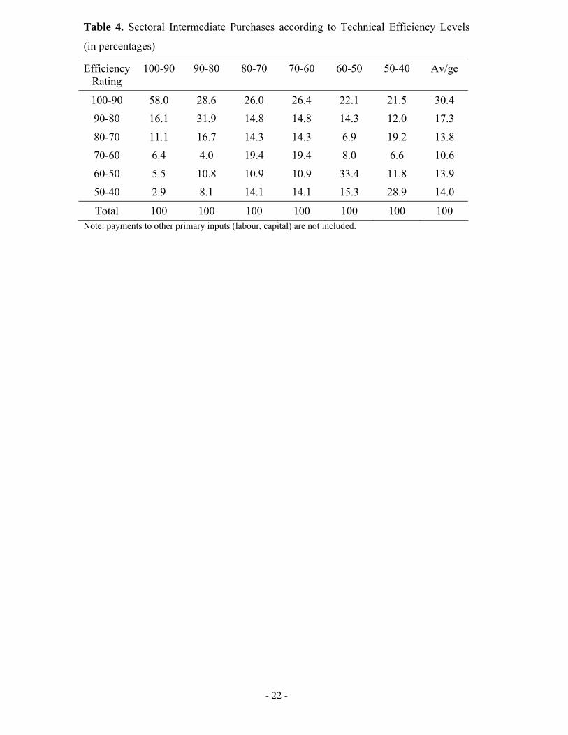
Table 4. Sectoral Intermediate Purchases according to Technical Efficiency Levels

(in percentages)

Efficiency Rating

100-90 90-80 80-70 70-60 60-50 50-40 Av/ge

100-90 58.0 28.6 26.0 26.4 22.1 21.5 30.4

90-80 16.1 31.9 14.8 14.8 14.3 12.0 17.3

80-70 11.1 16.7 14.3 14.3 6.9 19.2 13.8 70-60 6.4 4.0 19.4 19.4 8.0 6.6 10.6

60-50 5.5 10.8 10.9 10.9 33.4 11.8 13.9

50-40 2.9 8.1 14.1 14.1 15.3 28.9 14.0

Total 100 100 100 100 100 100 100 Note: payments to other primary inputs (labour, capital) are not included.

- 22 -

Table 5. Intermediate Purchases of the Ten Most and Least Efficient Sectors

According to the Technical Efficiency Level of the Supply Sectors (in percentages)

Efficiency Ten Most Technically Efficient Sectors

Rating 71A 69A 78 69B 70B 77A 77B 11 70A 73C

Own 0.0 8.8 0.4 1.2 50.9 6.2 1.2 0.1 36.8 19.6

100-90 92.5 40.5 30.3 52.0 32.7 52.6 60.6 35.6 34.7 33.4

90-80 0.2 24.4 26.8 18.8 11.2 26.5 23.3 10.3 19.1 24.0

80-70 6.2 15.8 28.6 24.1 3.7 10.2 11.3 5.8 7.5 11.2 70-60 0.0 4.0 2.4 2.3 1.1 2.2 2.0 23.7 1.4 4.7

60-50 0.5 3.0 1.7 0.7 0.3 1.1 0.8 18.4 0.4 5.1

50-40 0.6 3.5 9.8 0.9 0.1 1.2 0.8 6.1 0.1 2.0

Total 100 100 100 100 100 100 100 100 100 100

Ten Least Technically Efficient Sectors

30 38 05+06 27B 43 28 46 07 25 17

Own 1.8 33.5 19.4 11.4 7.3 3.3 1.9 11.3 0.2 3.2

100-90 12.9 6.5 12.1 10.5 15.9 17.6 21.2 15.6 14.6 12.4

90-80 9.9 8.2 14.1 18.1 8.2 16.3 8.4 14.1 11.4 9.2

80-70 39.7 2.7 13.4 10.9 2.7 51.3 3.0 9.4 32.6 6.9

70-60 3.1 11.0 0.4 5.3 11.0 3.5 16.8 5.2 34.8 2.6

60-50 0.1 16.3 11.3 0.0 31.1 0.2 34.2 12.1 1.9 27.1

50-40 32.5 21.8 29.3 43.8 23.8 7.8 14.5 32.3 4.5 38.6

Total 100 100 100 100 100 100 100 100 100 100 Note: payments to other primary inputs (labour, capital) are not included.

- 23 -

Endnotes 1 Ghosh (1958) and Augustinovics (1970) used the same approach to describe the

supply-driven input-output model. Under the usual assumptions the output vector is

determined exogenously by the primary input vector V. 2 Promising methodological improvements of the Strassert extraction method were

also suggested by Cella (1984) and Sonis et al. (1995). However, the proposed

backward and forward linkages are not symmetrical and thus they are comparable to

the corresponding traditional linkage indicators of Chenery and Watanabe (1958)

and Rasmussen (1956). 3 In cases when a sector j purchases no inputs from any other sector in the economy,

the total absolute backward linkage is zero and the actual situation is exactly the

same as the hypothesized one. 4 The use of the supply-driven Input-Output system for the computation of forward

linkages dispenses with the restrictive assumption of the Hirschmanian forward

linkages according to which the demand of every other industry increases

simultaneously (Augustinovics, 1970). However, since the inverted matrix

represents the sectoral sales shares and not the technology of production, forward

linkages computed using the supply-driven system are mutually inconsistent with

backward linkages computed using the demand-driven system (Cella, 1984;

Heimler, 1991). 5 Imports were treated as an input in the production process since they are often used

as raw materials or intermediate goods, while even in the case that refers to finished

products they have value added domestically through transportation and retailing

costs (Kohli, 1991). 6 The corresponding likelihood ratio tests are not presented herein but are available

upon request. 7 Notice that the probability of the technical inefficiency effect being significant in

the stochastic frontier model is high, since the estimated value of the γ -parameter is

close to one (see Table 1).

- 24 -