Second International Workshop on

Formal Techniques for Safety-Critical Systems

(FTSCS 2013)

Preliminary Proceedings

Editors: Cyrille Artho and Peter Csaba Olveczky

Preface

This volume contains the preliminary proceedings of the Second InternationalWorkshop of Formal Techniques for Safety-Critical Systems (FTSCS 2013), heldin Queenstown, New Zealand, on October 29–30, 2013, as a satellite event of theICFEM conference.

The aim of this workshop is to bring together researchers and engineerswho are interested in the application of formal and semi-formal methods toimprove the quality of safety-critical computer systems. FTSCS strives strivesto promote research and development of formal methods and tools for industrialapplications, and is particularly interested in industrial applications of formalmethods. Specific topics include, but are not limited to:

– case studies and experience reports on the use of formal methods for ana-lyzing safety-critical systems, including avionics, automotive, medical, andother kinds of safety-critical and QoS-critical systems;

– methods, techniques and tools to support automated analysis, certification,debugging, etc., of complex safety/QoS-critical systems;

– analysis methods that address the limitations of formal methods in industry(usability, scalability, etc.);

– formal analysis support for modeling languages used in industry, such asAADL, Ptolemy, SysML, SCADE, Modelica, etc.; and

– code generation from validated models.

The workshop received 33 submissions; 32 of these were regular papers and 1was a work-in-progress/position paper. Each submission was reviewed by threereferees; based on the reviews and extensive discussions, the program committeeselected 17 regular papers and one work-in-progress paper for presentation at theworkshop and inclusion in this volume. In addition, our program also includesan invited talk by Ian Hayes.

Revised versions of accepted regular papers will appear in the post-procee-dings of FTSCS 2013 that will be published as a volume in Springer’s Communi-cations in Computer and Information Science (CCIS) series. Extended versionsof selected papers from the workshop will also appear in a special issue of theScience of Computer Programming journal.

Many colleagues and friends have contributed to FTSCS 2013. First, wewould like to thank Kokichi Futatsugi and Hitoshi Ohsaki for initiating thisseries of workshops. We thank Ian Hayes for accepting our invitation to give aninvited talk and the authors who submitted their work to FTSCS 2013 and who,through their contributions, make this workshop an interesting event. We areparticularly grateful that so many well known researchers agreed to serve on theprogram committee, and that they all provided timely, insightful, and detailedreviews.

We also thank the editors of Communications in Computer and InformationScience for agreeing to publish the proceedings of FTSCS 2013 as a volume intheir series, and Jan A. Bergstra and Bas van Vlijmen for accepting our proposalto devote a special issue of the Science of Computer Programming journal to

I

extended versions of selected papers from FTSCS 2013. Furthermore, Jing Sunhas been very helpful with the local arrangements. Finally, we thank AndreiVoronkov for the excellent EasyChair conference systems.

We hope that you will all enjoy both the scientific program and the workshopvenue!

October, 2013 Cyrille ArthoPeter Csaba Olveczky

II

Workshop Organization

Workshop Chair

Hitoshi Ohsaki AIST

Program Chairs

Cyrille Artho AIST

Peter Csaba Olveczky University of Oslo

Program Committee

Erika Abraham RWTH Aachen UniversityMusab Alturki King Fahd University of Petroleum and MineralsToshiaki Aoki JAISTFarhad Arbab Leiden University and CWICyrille Artho AISTSaddek Bensalem VerimagArmin Biere Johannes Kepler UniversitySantiago Escobar Universidad Politecnica de ValenciaAnsgar Fehnker University of the South PacificMamoun Filali IRITBernd Fischer Stellenbosch University/University of SouthamptonKokichi Futatsugi JAISTKlaus Havelund NASA JPL/California Institute of TechnologyMarieke Huisman University of TwenteRalf Huuck NICTAFuyuki Ishikawa National Institute of InformaticsTakashi Kitamura AISTAlexander Knapp Augsburg UniversityPaddy Krishnan Oracle Labs BrisbaneYang Liu Nanyang Technological UniversityRobi Malik University of WaikatoCesar Munoz NASA LangleyTang Nguyen Hanoi University of IndustryThomas Noll RWTH Aachen University

Peter Olveczky University of OsloPaul Pettersson Malardalen UniversityCamilo Rocha Escuela Colombiana de IngenieriaGrigore Rosu University of Illinois at Urbana-Champaign

III

Neha Rungta NASA Ames Research CenterRalf Sasse ETH ZurichOleg Sokolsky University of PennsylvaniaSofiene Tahar Concordia UniversityCarolyn Talcott SRI InternationalTatsuhiro Tsuchiya Osaka UniversityMichael Whalen University of MinnesotaPeng Wu Chinese Academy of Sciences

External Reviewers

Daghar, Alaeddine Elleuch, MaissaEnoiu, Eduard Paul Helali, GhassenJansen, Nils Kong, WeiqiangMeredith, Patrick Rongjie, YanSantiago, Sonia

IV

Table of Contents

Towards Structuring System Specifications with Time Bands UsingLayers of Rely-Guarantee Conditions . . . . . . . . . . . . . . . . . . . . . . . . . . . . . . . . 1

Ian J. Hayes

Certainly Unsupervisable States . . . . . . . . . . . . . . . . . . . . . . . . . . . . . . . . . . . . 3

Simon Ware, Robi Malik, Sahar Mohajerani and Martin Fabian

Wind Turbine System: An Industrial Case Study in Formal Modelingand Verification . . . . . . . . . . . . . . . . . . . . . . . . . . . . . . . . . . . . . . . . . . . . . . . . . . . 19

Jagadish Suryadevara, Gaetana Sapienza, Cristina Seceleanu, TiberiuSeceleanu, Stein Erik Ellevseth and Paul Pettersson

Precise Documentation and Validation of Requirements . . . . . . . . . . . . . . . . 35

Chen-Wei Wang, Jonathan Ostroff and Simon Hudon

Reflections on Verifying Software with Whiley . . . . . . . . . . . . . . . . . . . . . . . . 51

David Pearce and Lindsay Groves

An UPPAAL Framework for Model Checking Automotive Systemswith FlexRay Protocol . . . . . . . . . . . . . . . . . . . . . . . . . . . . . . . . . . . . . . . . . . . . . 67

Xiaoyun Guo, Hsin-Hung Lin, Kenro Yatake and Toshiaki Aoki

Early Analysis of Soft Error Effects for Aerospace Applications usingProbabilistic Model Checking . . . . . . . . . . . . . . . . . . . . . . . . . . . . . . . . . . . . . . . 83

Khaza Anuarul Hoque, Otmane Ait Mohamed, Yvon Savaria and ClaudeThibeault

TTM/PAT: Specifying and Verifying Timed Transition Models . . . . . . . . . 99

Jonathan Ostroff, Chen-Wei Wang, Yang Liu, Jun Sun and SimonHudon

On the cloud-enabled refinement checking of railway signallinginterlockings . . . . . . . . . . . . . . . . . . . . . . . . . . . . . . . . . . . . . . . . . . . . . . . . . . . . . 115

Andrew Simpson and Jaco Jacobs

Counterexample generation for hybrid automata . . . . . . . . . . . . . . . . . . . . . . 131

Johanna Nellen, Erika Abraham, Xin Chen and Pieter Collins

Compositional Nonblocking Verification with Always Enabled Eventsand Selfloop-only Events . . . . . . . . . . . . . . . . . . . . . . . . . . . . . . . . . . . . . . . . . . . 147

Colin Pilbrow and Robi Malik

Formalizing and Verifying Function Blocks using Tabular Expressionsand PVS . . . . . . . . . . . . . . . . . . . . . . . . . . . . . . . . . . . . . . . . . . . . . . . . . . . . . . . . . 163

Linna Pang, Chen-Wei Wang, Mark Lawford and Alan Wassyng

V

Parametric Schedulability Analysis of Fixed Priority Real-TimeDistributed Systems . . . . . . . . . . . . . . . . . . . . . . . . . . . . . . . . . . . . . . . . . . . . . . . 179

Youcheng Sun, Romain Soulat, Giuseppe Lipari, Etienne Andre andLaurent Fribourg

Model Based Testing from Controlled Natural Language Requirements . . . 195Gustavo Carvalho, Flavia Barros, Florian Lapschies, Uwe Schulze andJan Peleska

Refinement Tree and Its Patterns: a Graphical Approach for Event-BModeling . . . . . . . . . . . . . . . . . . . . . . . . . . . . . . . . . . . . . . . . . . . . . . . . . . . . . . . . 211

Kriangkrai Traichaiyaporn and Toshiaki Aoki

Formal Semantics and Analysis of Timed Rebeca in Real-Time Maude . . . 227Zeynab Sabahi Kaviani, Ramtin Khosravi, Marjan Sirjani, Peter Olveczkyand Ehsan Khamespanah

A Strand Space Approach to Provable Anonymity . . . . . . . . . . . . . . . . . . . . . 243Yongjian Li and Jun Pang

Creating Visualisations of Formal Models of Interactive Medical Devices . 259Judy Bowen, Steve Reeves and Steve Jones

With an Open Mind: How to Write Good Models . . . . . . . . . . . . . . . . . . . . . 264Cyrille Valentin Artho, Koji Hayamizu, Rudolf Ramler and YoriyukiYamagata

VI

Towards Structuring System Specifications withTime Bands Using Layers of Rely-Guarantee Conditions

Ian J. Hayes

School of ITEE, The University of Queensland, Brisbane, Australia

Abstract. The overall specification of a cyber-physical system can be given interms of the desired behaviour of its physical components operating within thereal world. The specification of its control software can then be derived from theoverall specification and the properties of the real-world phenomena, includingtheir relationship to the computer system’s sensors and actuators. The controlsoftware specification them becomes a combination of the guarantee it makesabout the system behaviour and the real-world assumptions it relies upon.Such specifications can easily become complicated because the complete systemdescription deals with properties of phenomena at widely different time granu-larities, as well as handling faults. To help manage this complexity, we considerlayering the specification within multiple time bands, with the specification ofeach time band consisting of both the rely and guarantee conditions for that band,both given in terms of the phenomena of that band. The overall specification isthen the combination of the multiple rely-guarantee pairs. Multiple rely-guaranteepairs can also be used to handle faults.

Rely-guarantee specifications. Earlier research with Michael Jackson and Cliff Jones[3, 4] looked at specifying real-time control systems in terms of assumptions about thebehaviour of the system’s environment – a rely condition – and the behaviour to be en-sured by the system – a guarantee condition – provided its environment ensures the relycondition continues to hold. Often the specification of the system’s desired behaviouris best described in terms of the behaviour of physical objects in the real-world thatare to be controlled by the computer system and rely conditions are needed to link thereal-world phenomena (which may not be directly accessible to the computer) to thecomputer’s view of the world, i.e. the computer’s sensors and actuators.

Multiple rely-guarantee pairs. Our earlier work [4] allowed a specification to be struc-tured into multiple rely-guarantee pairs, where each guarantee is paired with a relycondition expressing the assumptions about the behaviour of the environment neededto be able to achieve that guarantee. This allows one to separate different aspects of thebehaviour of a system so that each guarantee is paired with its corresponding rely. Italso allows one to separate the specification of “normal” behaviour of the system whenthe environment is behaving correctly according to the normal rely, and a fall-back ordegraded mode of behaviour when the normal rely condition does not hold but a weakerrely does hold.

1

The time bands framework. Too often when describing of a system’s specification (orrequirements), the basic operation of the system gets lost in a plethora of low-leveldetail. For real-time systems it has been observed that it helps to view the system atmultiple time bands or scales [1, 2]. The phenomena relevant at one time band maybe different to those at a finer-grained (lower) time band. The behaviour of a systemmay be specified by describing aspects of the behaviour separately for each time bandin terms of the phenomena of that band. For example, an “instantaneous” event at onetime band may correspond to an activity consisting of a set of events (occurring closetogether) at the next lower time band. Events at the lower time band may be defined interms of phenomena only “visible” at that time band.

Rely-guarantee for each time band. The specification of the behaviour for each timeband can be given in terms of a rely condition giving assumed properties of the environ-ment and a guarantee of the behaviour of the system, both in terms of the phenomena ofthe time band. In this way the behaviour of the overall system is described in terms ofmultiple rely-guarantee pairs (as described above) with at least one rely-guarantee pairfor each time band used in structuring the description of the system behaviour.

Acknowledgements. The research presented here is based on joint research with AlanBurns, Brijesh Dongol, Michael Jackson and Cliff Jones. The author’s research wassupported by Australian Research Council Grants DP0987452 and DP130102901.

References

1. Alan Burns and Gordon Baxter. Time bands in systems structure. In D. Besnard, C. Gacek,and C. B. Jones, editors, Structure for Dependability: Computer-Based Systems from an In-terdisciplinary Perspective, pages 74–90. Springer, 2006.

2. Alan Burns and Ian J. Hayes. A timeband framework for modelling real-time systems. Real-Time Systems, 45(1–2):106–142, June 2010.

3. I.J. Hayes, M.A. Jackson, and C.B. Jones. Determining the specification of a control systemfrom that of its environment. In K. Araki, S. Gnesi, and D. Mandrioli, editors, FME 2003:Formal Methods, volume 2805 of LNCS, pages 154–169. Springer Verlag, 2003.

4. Cliff B. Jones, Ian J. Hayes, and Michael A. Jackson. Deriving specifications for systemsthat are connected to the physical world. In Jim Woodcock, editor, Essays in Honour of DinesBjørner and Zhou Chaochen on the Occassion of their 70th Birthdays, volume 4700 of LectureNotes in Computer Science, pages 364–390. Springer Verlag, 2007.

2

Certainly Unsupervisable States

Simon Ware1, Robi Malik1, Sahar Mohajerani2, and Martin Fabian2

1 Department of Computer Science,University of Waikato, Hamilton, New Zealand

{siw4,robi}@waikato.ac.nz2 Department of Signals and Systems,

Chalmers University of Technology, Gothenburg, Sweden{mohajera,fabian}@chalmers.se

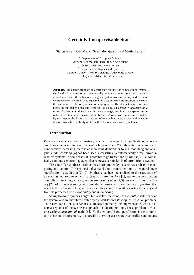
Abstract. This paper proposes an abstraction method for compositional synthe-sis.Synthesisis a method to automatically compute acontrol programor super-visor that restricts the behaviour of a given system to ensure safety and liveness.Compositional synthesisuses repeated abstraction and simplification to combatthe state-space explosion problem for large systems. The abstraction method pro-posed in this paper finds and removes the so-calledcertainly unsupervisablestates. By removing these states at an early stage, the final state space can bereduced substantially. The paper describes an algorithm with cubic time complex-ity to compute the largest possible set of removable states. A practical exampledemonstrates the feasibility of the method to solve real-world problems.

1 Introduction

Reactive systemsare used extensively to control safety-critical applications, where asmall error can result in huge financial or human losses. Withtheir size and complexitycontinuously increasing, there is an increasing demand forformal modelling and anal-ysis.Model checking[4] has been used successfully to automatically detect errors inreactive systems. In some cases, it is possible to go furtherandsynthesise, i.e., automat-ically compute a controlling agent that removes certain kinds of errors from a system.

The controller synthesis problem has been studied by several researchers in com-puting and control. The synthesis of a stand-alone controller from a temporal logicspecification is studied in [7, 19]. Synthesis has been generalised to the extraction ofan environment to interact with a given softwareinterface[1], and to the constructioncontrollers interacting with a givenenvironmentor plant [2,5]. Supervisory control the-ory [20] of discrete event systems provides a framework to synthesise asupervisorthatrestricts the behaviour of a given plant as little as possible while ensuring the safety andliveness properties ofcontrollability andnonblocking.

Straightforward synthesis algorithms explore the completemonolithicstate space ofthe system, and are therefore limited by the well-knownstate-space explosionproblem.The sheer size of the supervisor also makes it humanly incomprehensible, which hin-ders acceptance of the synthesis approach in industrial settings. These problems are ad-dressed bycompositionalmethods [3,8]. If a temporal logic specification is the conjunc-tion of several requirements, it is possible to synthesise separate controller components

3

for each requirement [5, 7]. Compositional approaches in supervisory control [9, 16]exploit the structure of the model of the plant to be controlled, which typically consistsof several interacting components. These approaches avoidconstructing the full statespace by first simplifying individual components, then applying synchronous composi-tion step by step, and simplifying the intermediate resultsagain.

This kind of compositional synthesis requires specific abstraction methods to guar-antee a least restrictive, controllable, and nonblocking final synthesis result.Supervisionequivalence[9] andsynthesis abstraction[16] have been proposed for this purpose, andseveral abstraction methods to simplify automata preserving these properties are known.

This paper proposes another abstraction method that can be used in compositionalsynthesis frameworks such as [9,16]. The proposed method finds all the states that willcertainly be removed by any supervisor. Removing these so-called certainly unsuper-visable statesat an early stage reduces the state space substantially. Previously,halfwaysynthesis[9] was used for this purpose, which approximates the removable states. Theset of certainly unsupervisable states is the largest possible set of removable states, andit can be computed in the same cubic complexity as halfway synthesis.

This paper is organised as follows. Section 2 introduces theterminology of super-visory control theory [20] and the framework of compositional synthesis [9, 16]. Next,Section 3 explains the ideas of compositional synthesis andcertainly unsupervisablestates using the example of a manufacturing system. Section4 presents the results ofthis paper: it defines the set of certainly unsupervisable states, gives an algorithm tocompute it, performs complexity analysis, and compares certainly unsupervisable statesto halfway synthesis. Finally, Section 5 adds some concluding remarks.

2 Preliminaries

2.1 Events and Languages

Discrete event systems are modelled using events and languages [20].Eventsrepresentincidents that cause transitions from one state to another and are taken from a finitealphabetΣ. For the purpose of supervisory control, the alphabet is partitioned into twodisjoint subsets, the setΣc of controllableevents and the setΣu of uncontrollableevents.Controllable events can be disabled by a supervising agent,while uncontrollable eventsoccur spontaneously. In addition, thesilent controllableeventτc ∈ Σc and thesilentuncontrollableeventτu ∈ Σu denote transitions that are not taken by any componentother than the one being considered. The set of all finitetracesof events fromΣ, in-cluding theempty traceε, is denoted byΣ∗. A subsetL⊆ Σ∗ is called alanguage. Theconcatenationof two tracess, t ∈ Σ∗ is written asst.

2.2 Nondeterministic Automata

System behaviours are typically modelled by deterministicautomata, but nondetermin-istic automata may arise as intermediate results during abstraction.

Definition 1. A (nondeterministic) finite automaton is a tupleG= 〈Σ,Q,→,Q◦,Qω〉,whereΣ is a finite set of events,Q is a finite set ofstates,→ ⊆ Q×Σ×Q is thestate

4

H1

fetch1 !put1

B1

!put1

!put1

!put1

get1

get1

⊥

H1 ‖B1 0

1 2

3 4

5

6 7fetch1

fetch1

fetch1

fetch1

!put1

!put1

!put1

get1 get1

get1

get1

S 0

1 2

3 4

fetch1

fetch1

!put1

!put1get1

get1get1

Fig. 1. Simple manufacturing system. Eventsfetch1 andget1 are controllable, while !put1 isuncontrollable.

transition relation, Q◦ ⊆Q is the set ofinitial states, andQω ⊆Q is the set ofaccepting

states. G is deterministicif |Q◦| ≤ 1 andτu,τc /∈ Σ, and for all transitionsxσ→ y1 and

xσ→ y2 it holds thaty1 = y2.

The transition relation is written in infix notationxσ→ y, and is extended to traces

and languages in the standard way. For example,xτ∗uσ−−→ y means that there exists a

possibly empty sequence ofτu-transitions followed by aσ -transition that leads fromstatex to y. Furthermore,x

s→ meansxs→ y for somey ∈ Q, andx→ y meansx

s→ yfor somes∈ Σ∗. These notations also apply to state sets and to automata:X

s→ Y forX,Y ⊆Q meansx

s→ y for somex∈ X andy∈Y, andGs→ x meansQ◦ s→ x.

Example 1. Fig. 1 shows automata models of a simple manufacturing system consist-ing of a handlerH1 and a bufferB1. The handler fetches a workpiece (fetch1) and thenputs it into the buffer (!put1). The event !put1 also increases the number of workpiecesin the buffer by 1. Afterwards the buffer can release the workpiece (get1), reducing thenumber of workpieces in the buffer by 1. The buffer can store only two workpieces,adding more workpieces causes overflow as represented by thestate⊥.

Definition 2. Let G1 = 〈Σ1,Q1,→1,Q◦1,Q

ω1 〉 and G2 = 〈Σ2,Q2,→2,Q

◦2,Q

ω2 〉 be two

automata. Thesynchronous compositionof G1 andG2 is

G1‖G2 = 〈Σ1∪Σ2,Q1×Q2,→,Q◦1×Q◦2,Qω1 ×Qω

2 〉 (1)

where

– (x1,x2)σ→ (y1,y2), if σ ∈ (Σ1∩Σ2)\{τu,τc}, x1

σ→1 y1, andx2σ→2 y2;

– (x1,x2)σ→ (y1,x2), if σ ∈ (Σ1\Σ2)∪{τu,τc} andx1

σ→1 y1;– (x1,x2)

σ→ (x1,y2), if σ ∈ (Σ2\Σ1)∪{τu,τc} andx2σ→2 y2.

Automata are synchronised in lock-step synchronisation [11]. Shared events mustbe executed by all automata together, while events used by only one automaton (andthe silent eventsτu andτc) are executed by only that automaton. Fig. 1 shows the syn-chronous compositionH1‖B1 of the automata mentioned in Example 1.

Another common operation in compositional synthesis ishiding, which removes theidentity of certain events and in general produces a nondeterministic automaton.

5

Definition 3. Let G = 〈Σ,Q,→,Q◦,Qω〉 be an automaton andϒ ⊆ Σ. The result ofcontrollability preserving hidingof ϒ from G is G\! ϒ = 〈Σ\ϒ,Q,→! ,Q

◦,Qω〉, where

→! is obtained from→ by replacing each transitionxσ→ y such thatσ ∈ ϒ by x

τc→ y ifσ ∈ Σc or byx

τu→ y if σ ∈ Σu.

2.3 Supervisory Control Theory

Supervisory control theory[20] provides a means to automatically compute so-calledsupervisorsthat control a given system to perform some desired functionality. Givenan automaton model of the possible behaviour of a physical system, called theplant, asupervisor is sought to restrict the behaviour in such a way that only a certain subset ofthe state space is reachable. The supervisor is implementedas acontrol function[20]

Φ : Q→ 2Σ×Q (2)

that assigns to each statex∈Q the setΦ(x) of transitions to be enabled in this state. Thatis, a transitionx

σ→ y with σ ∈ Σc will only be possible under the control of supervisorΦif (σ ,y) ∈ Φ(x). Uncontrollable events cannot be disabled, so it is required thatΣu×Q⊆ Φ(x) for all x ∈ Q. Controllable transitions can be disabled individually, i.e., ifa nondeterministic system contains multiple outgoing controllable transitions from astatex, then the supervisor may disable some of them while leaving others enabled [9].If the plant is modelled by a nondeterministic automaton, then such a supervisor can berepresented as asubautomaton.

Definition 4. [9] Let G= 〈Σ,QG,→G,Q◦G,QωG〉 andK = 〈Σ,QK ,→K ,Q◦K ,Qω

K 〉 be twoautomata.K is asubautomatonof G, writtenK ⊆G, if QK ⊆QG,→K ⊆→G, Q◦K ⊆Q◦G,andQω

K ⊆QωG.

A subautomatonK of G contains a subset of the states and transitions ofG. It rep-resents a supervisor that enables only those transitions present inK, i.e., it implementsthe control function

ΦK(x) = (Σu×Q)∪{(σ ,y) ∈ Σc×Q | x σ→K y} . (3)

As uncontrollable events cannot be disabled, the control function includes all possi-ble uncontrollable transitions. Then not every subautomaton of G can be implementedthrough control. The property ofcontrollability [20] characterises those behaviours thancan be implemented.

Definition 5. [9] Let G = 〈Σ,QG,→G,Q◦G,QωG〉 andK = 〈Σ,QK ,→K ,Q◦K ,Qω

K 〉 suchthatK ⊆G. ThenK is calledcontrollablein G if, for all statesx∈QK andy∈QG andfor every uncontrollable eventυ ∈ Σu such thatx

υ→G y, it also holds thatxυ→K y.

If a subautomatonK is controllable inG, then every uncontrollable transition pos-sible inG is also contained inK. In Fig. 1, automatonS is controllable inH1‖B1. How-ever, if state 5 was to be included inS, then because of the uncontrollable transition

6

5!put1−−−→ 6, state 6 would also have to be included forS to be controllable. Controlla-

bility ensures that the control function (3) can be implemented without disabling anyuncontrollable events.

In addition to controllability, the supervised behaviour is typically required to benonblocking.

Definition 6. [15] Let G= 〈Σ,Q,→,Q◦,Qω〉 be an automaton.G is callednonblock-ing if for every statex∈Q such thatQ◦→ x it holds thatx→Qω .

In a nonblocking automaton, termination is possible from every reachable state. Thenonblocking property, also referred to asweak termination[17], ensures the absenceof livelocks and deadlocks. Combined with controllability, the requirement to be non-blocking can express arbitrary safety properties [9]. For example, the buffer modelB1

in Fig. 1 contains the !put1-transition to the blocking state⊥ to specify a supervised be-haviour that does not allow a third workpiece to be placed into the buffer when it alreadycontains two workpieces, i.e., it requests a supervisor that prevents buffer overflow.

Given a plant automatonG, the objective ofsupervisor synthesis[20] is to com-pute a subautomatonK ⊆ G, which is controllable and nonblocking and restricts thebehaviour ofG as little as possible. The set of subautomata ofG forms a lattice [6], andthe upper bound of a set of controllable and nonblocking subautomata in this lattice isagain controllable and nonblocking.

Theorem 1. [9] Let G = 〈Σ,Q,→,Q◦,Qω〉 be an automaton. There exists a uniquesubautomaton supC(G) ⊆ G such that supC(G) is nonblocking and controllable inG,and such that for every subautomatonS⊆ G that is also nonblocking and controllablein G, it holds thatS⊆ supC(G).

The subautomaton supC(G) is the uniqueleast restrictivesub-behaviour ofG thatcan be achieved by any possible supervisor. It can be computed using a fixpoint itera-tion [9], by iteratively removing blocking states and states leading to blocking states viauncontrollable events, until a fixpoint is reached.

Definition 7. [9] Let G= 〈Σ,Q,→,Q◦,Qω〉 be an automaton. Therestrictionof G toX ⊆Q is G|X = 〈Σ,X,→|X,Q◦∩X,Qω ∩X〉, where→|X = {(x,σ ,y) ∈→ | x,y∈ X}.Definition 8. [9] Let G= 〈Σ,Q,→,Q◦,Qω〉 be an automaton. Thesynthesis stepop-eratorΘG : 2Q→ 2Q for G is defined asΘG(X) = Θcont

G (X)∩ΘcontG (X), where

ΘcontG (X) = {x∈ X | for all transitionsx

υ→ y with υ ∈ Σu it holds thaty∈ X} ; (4)

ΘnonbG (X) = {x∈ X | x→|X Qω } . (5)

ΘcontG captures controllability, andΘnonb

G captures nonblocking. The least restrictivesynthesis result supC(G) is obtained by restrictingG to the greatest fixpoint ofΘG.

Theorem 2. [9] Let G = 〈Σ,Q,→,Q◦,Qω〉. The synthesis step operatorΘG has agreatest fixpoint gfpΘG = ΘG ⊆ Q, such thatG|ΘG

is the greatest subautomaton ofGthat is both controllable inG and nonblocking, i.e.,

supC(G) = G|ΘG. (6)

7

Example 2. The automatonH1‖B1 in Fig. 1 is blocking, because the tracefetch1!put1fetch1!put1fetch1!put1 leads to state 6, from where no accepting state is reachable.Toprevent this blocking situation, event !put1 needs to be disabled in state 5. However,!put1 is an uncontrollable event that cannot be disabled by the supervisor, so the bestfeasible solution is to disable the controllable eventfetch1 in state 3. Fig. 1 shows theleast restrictive supervisorS= supC(H1‖B1).

In the finite-state case, the state set of the least restrictive supervisor can be calcu-lated as the limit of the sequenceX0 = Q, Xi+1 = ΘG(Xi). This iteration converges inat most|Q| iterations, and the worst-case time complexity isO(|Q||→|) = O(|Σ||Q|3),where|Σ|, |Q|, and|→| are the numbers of events, states, and transitions of the plantautomatonG. However, often the behaviour the system is specified by a large num-ber of synchronised automata, and when measured by the number of components, thesynthesis problem is NP-complete [10].

2.4 Compositional Synthesis

Many discrete event systems aremodularin that they consist of a large number of inter-acting components. This modularity allows to simplify individual components beforecomposing them, in many cases avoiding state-space explosion. This idea has been usedsuccessfully for verification of large discrete event systems [8].

Given a system of concurrent plant automata

G = G1‖G2‖ · · · ‖Gn , (7)

the objective of synthesis is to find a least restrictive supervisor, which ensures non-blocking without disabling uncontrollable events. The standard solution [20] to thisproblem is to calculate a finite-state representation of thesynchronous composition (7)and use a synthesis iteration to calculate supC(G ) = supC(G1‖ · · · ‖Gn).

A compositional algorithm tries to find the same result without explicitly calculatingthe synchronous product (7). It seeks to abstract individual automataGi by removingsome states or transitions, and replace them by abstracted versionsGi . If no more ab-straction is possible, synchronous composition is computed step by step, abstracting theintermediate results again.

The individual automataGi typically contain some events that do not appear in anyother automataG j . These events are calledlocal events, denoted by the setϒ in thefollowing. After hiding the local events, the automatonGi is replaced byGi \! ϒ, whichincreases the possibility of further abstraction.

Eventually, the procedure leads to a single automatonG, the abstract descriptionof the systemG . After abstraction, the automaton ofG has less states and transitionscompared to (7). OnceG is found, the final step is to use it instead of the originalsystem, to obtain a synthesis result supC(G) = supC(G ).

The abstraction steps to simplify the individual automataGi must satisfy certainconditions to guarantee that the synthesis result obtainedfrom the final abstraction is acorrect supervisor for the original system.

8

M2

M1

!put2

B2

!put1

B1

!put3

H3

!put4

H4

H1 H2B3 B4

get3fetch2fetch1 get4

get2get1 fetch3 fetch4

input2 !output2

!output1 input1

W1

Fig. 2.Manufacturing system overview.

W1 Lock Produce M1 M2

⊥!output1

!output1!res

!sus

!lock

!res!sus

!lock unlock

⊥!output1

!output1

!output1input1

!output1

fetch1

fetch2

get3

get4

input2 fetch4

fetch3

get2 !output2

get1

Fig. 3.Automata for manufacturing system model. Uncontrollable events are prefixed by !.

Definition 9. Let G and H be two automata with alphabetΣ. ThenG is a synthesisequivalentto H, writtenG≃synthH, if for every automatonT = 〈ΣT ,QT ,→T ,Q◦T ,Qω

T 〉it holds that supC(G‖T) = supC(H ‖T).

Def. 9 is a special case of synthesis abstraction [16]. Synthesis equivalence requiresthat the abstracted automatonH yields the same supervisor as the original automatonG,no matter what the remainder of the systemT is.

3 Manufacturing System Example

This section demonstrates compositional synthesis using amodified version of a manu-facturing system previously studied in [13]. The manufacturing system consists of twomachines (M1 andM2) and four pairs of handlers (Hi) and buffers (Bi) for transferringworkpieces between the machines. Fig. 2 gives an overview ofthe system.

The manufacturing system can produce two types of workpieces. Type I workpiecesare first processed by machineM1 (input1). Then they are fetched by handlerH1 (fetch1)and placed into bufferB1 (!put1). Next, they are processed byM2 (get1), fetched byH4

(fetch4) and placed intoB4 (!put4). Finally, they are processed byM1 once more (get4),and released (!output1). Using a switchW1, users can request to suspend (!sus) or re-sume (!res) production ofM1, provided that the switch has been unlocked (unlock) bythe system. Type II workpieces are first processed byM2, passed throughH3 andB3,further processed byM1, passed throughH2 andB2, and finally processed byM2. Thehandlers and buffers are modelled as in Fig. 1, and Fig. 3 shows the rest of the automatamodel of the system. AutomataW1 andProduceuse the blocking states⊥ to modelrequirements for the synthesised supervisor to prevent output fromM1 in suspend modeand to produce exactly two Type I workpieces.

9

HB1 0

1 2

3 4

5

⊥

fetch1

fetch1

fetch1

get1

get1

get1

get1

τu

τu

τu

W0

1

2

3

4

5

6

7

8

9

10

11

⊥1 ⊥2 ⊥3

!output1

!output1

!output1

!output1

!output1

!output1

!output1

!output1

!output1

!output1

!output1

!output1

τuτu τuτu τuτu

τuτu τu τc

τc τc

τc τc

τc

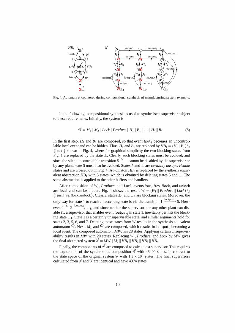
Fig. 4.Automata encountered during compositional synthesis of manufacturingsystem example.

In the following, compositional synthesis is used to synthesise a supervisor subjectto these requirements. Initially, the system is

G = M1‖M2‖Lock‖Produce‖H1‖B1‖ · · · ‖H4‖B4 . (8)

In the first step,H1 andB1 are composed, so that event !put1 becomes an uncontrol-lable local event and can be hidden. Thus,H1 andB1 are replaced byHB1 = (H1‖B1)\!{!put1} shown in Fig. 4, where for graphical simplicity the two blocking states fromFig. 1 are replaced by the state⊥. Clearly, such blocking states must be avoided, andsince the silent uncontrollable transition 5

τu→⊥ cannot be disabled by the supervisor orby any plant, state 5 must also be avoided. States 5 and⊥ arecertainly unsupervisablestatesand are crossed out in Fig. 4. AutomatonHB1 is replaced by the synthesis equiv-alent abstraction ˜HB1 with 5 states, which is obtained by deleting states 5 and⊥. Thesame abstraction is applied to the other buffers and handlers.

After composition ofW1, Produce, andLock, events !sus, !res, !lock, andunlockare local and can be hidden. Fig. 4 shows the resultW = (W1 ‖Produce‖ Lock) \!{!sus, !res, !lock,unlock}. Clearly, states⊥1 and⊥2 are blocking states. Moreover, the

only way for state 1 to reach an accepting state is via the transition 1!output1−−−−−→ 5. How-

ever, 1τu→ 2

!output1−−−−−→ ⊥1, and since neither the supervisor nor any other plant can dis-ableτu, a supervisor that enables event !output1 in state 1, inevitably permits the block-ing state⊥1. State 1 is a certainly unsupervisable state, and similar arguments hold forstates 2, 3, 5, 6, and 7. Deleting these states fromW results in the synthesis equivalentautomatonW. Next, M1 andW are composed, which results in !output1 becoming alocal event. The composed automaton,MW, has 28 states. Applying certain unsupervis-ability results inMW with 20 states. ReplacingW1, Produce, andLock by MW givesthe final abstracted systemG = MW‖M2‖ ˜HB1‖ ˜HB2‖ ˜HB3‖ ˜HB4.

Finally, the components ofG are composed to calculate a supervisor. This requiresthe exploration of the synchronous compositionG with 48400 states, in contrast tothe state space of the original systemG with 1.3× 106 states. The final supervisorscalculated fromG andG are identical and have 4374 states.

10

4 Certain Unsupervisability

4.1 Certainly Unsupervisable States and Transitions

The above example shows that some states of an automatonG must be avoided bysynthesis in every possible context. That is, no matter whatother automata are latercomposed withG, it is clear that these states are unsafe. Blocking states are examplesof such states, but there are more states with this property.

Definition 10. Let G= 〈Σ,Q,→,Q◦,Qω〉 be an automaton. Thecertainly unsupervis-able state setof G is

U(G) = {x∈Q | for every automatonT = 〈Σ,QT ,→T ,Q◦T ,QωT 〉 and every

statexT ∈QT it holds that(x,xT) /∈ ΘG‖T } .(9)

A statex of G is certainly unsupervisable, if there exists no other automaton Tsuch that the statex is present in the least restrictive synthesis resultΘG‖T . If a state iscertainly unsupervisable, it is known that this state will be removed by any synthesis. Ifsuch states are encountered in an automaton during compositional synthesis, they canbe removed before composing this automaton further.

Example 3. Consider again automatonHB1 in Fig. 4. Clearly, the blocking state⊥is certainly unsupervisable. In addition, state 5 is also certainly unsupervisable, be-cause of the local uncontrollable transition 5

τu→⊥. As this transition is silent, no othercomponent disables it, and as it is uncontrollable, the supervisor cannot disable it.Therefore, if the automaton ever enters state 5, blocking isunavoidable. It holds thatU(HB1) = {5,⊥}.

In addition to states, it is worth considering transitions as certainly unsupervisable.If an uncontrollable eventυ can take a statex to a certainly unsupervisable state, thenall υ-transitions fromx are certainly unsupervisable. Such transitions can be removedbecause it is clear that no supervisor will allow statex to be entered whileυ is possiblein the plant.

Definition 11. Let G = 〈Σ,Q,→,Q◦,Qω〉 be an automaton. A transitionxυ→ y with

υ ∈ Σu is acertainly unsupervisable transitionif xτ∗uυ−−→ U(G).

Example 4. Consider automatonW in Fig. 4. States⊥1, ⊥2, and⊥3 are blocking andtherefore certainly unsupervisable. State 5 is also certainly unsupervisable, because

every path from state 5 to an accepting state must take the transition 5!output1−−−−−→ 9.

However, this transition is certainly unsupervisable, as !output1 is uncontrollable and

5τu→ 6

!output1−−−−−→⊥2 ∈ U(W). The only way for a potential supervisor to avoid the block-ing state⊥2 is to also avoid state 5. By similar arguments, it follows that U(W) ={1,2,3,5,6,7,⊥1,⊥2,⊥3}.

If the certainly unsupervisable states and transitions areknown, they can be used tosimplify an automaton to form a synthesis equivalentabstraction.

11

Definition 12. Let G= 〈Σ,Q,→,Q◦,Qω〉 be an automaton. The result ofunsupervis-ability removalfrom G is the automaton

unsupC(G) = 〈Σ,Q,→unsup,Q◦ \U(G),Qω \U(G)〉 , (10)

where

→unsup= {(x,σ ,y) ∈→ | σ ∈ Σc andx,y /∈ U(G)}∪ (11)

{(x,υ ,y) ∈→ | υ ∈ Σu, x /∈ U(G), andy∈ U(G)}∪ (12)

{(x,υ ,y) ∈→ | υ ∈ Σu, x /∈ U(G), andxτ∗uυ−−→ U(G) does not hold} . (13)

All controllable transitions to unsupervisable states areremoved (11), as these tran-sitions can always be disabled by the supervisor and therefore never appear in the finalsynthesis result. Uncontrollable transitions to certainly unsupervisable states, however,are retained (12), because they are needed to inform future synthesis step. If anothercomponent disables these events, they may disappear in synchronous composition withthat component, otherwise the source state may have to be removed in synthesis. Uncon-trollable transitions to other states are deleted if they are certainly unsupervisable (13).

Example 5. When applied to automatonW in Fig. 4, unsupervisability removal deletesall transitions linked to the crossed out states. While state⊥3 is also certainly unsuper-visable, the shared uncontrollable !output1-transitions to this state are retained. Theyare needed in the following steps of compositional synthesis. If some other componentdisables !output1 while in state 10 or 11, then these states may be retained, otherwisethey will be removed at a later stage.

The following theorem confirms that unsupervisability removal results in a synthe-sis equivalent automaton. Therefore, the abstraction can be used to replace an automa-ton during compositional synthesis without affecting the final synthesis result.

Theorem 3. Let G be an automaton. ThenG≃synthunsupC(G).

Unsupervisability removal by definition only removes transitions and no states. Yet,states may become unreachable as a result of transition removal, and unreachable statescan always be removed. Furthermore, it is possible to combine all remaining unsuper-visable states, which have no outgoing transitions, into a single state [16].

4.2 Iterative Characterisation

The following definition provides an alternative characterisation of the certainly unsu-pervisable states through an iteration. It forms the basis for an algorithm to compute theset of certainly unsupervisable states.

12

Definition 13. Let G = 〈Σ,Q,→,Q◦,Qω〉 be an automaton. Define the setU(G) in-ductively as follows.

U0(G) = /0 ; (14)

Uk+1(G) = {x∈Q | for all pathsx= x0σ1→·· · σn→ xn∈Qω there existsi = 0, . . . ,n

such thatxiτ∗u→Uk(G) or i > 0 andσi ∈ Σu andxi−1

τ∗uσiτ∗u−−−−→Uk(G) } ;

(15)

U(G) =⋃

k≥0

Uk(G) . (16)

The setUk(G) contains unsupervisable states oflevel k. There are no unsupervis-able states of level 0, and the unsupervisable states of level 1 are the blocking states,i.e., those states from where it is not possible to ever reachan accepting state. Unsu-pervisable states at a higher level are states from where every path to an accepting stateis known to pass through an unsupervisable state or an unsupervisable transition of alower level.

Example 6. Consider automatonW in Fig. 4. It holds thatU0(W) = /0, andU1(W) ={⊥1,⊥2,⊥3} contains the three blocking states. Next, it can be seen that1∈U2(W),

because every path from 1 to an accepting state includes the transition 1!output1−−−−−→ 5 with

!output1 ∈ Σu and 1τu→ 2

!output1−−−−−→ ⊥1 ∈ U1(W). Likewise, it holds that 2,3,5,6,7 ∈U2(W). No further states are contained inU2(W) or inUk(W) for k> 2, so thatU(W)=U2(W) = {1,2,3,5,6,7,⊥1,⊥2,⊥3}= U(W).

The following Theorem 4 confirms that the iterationUk(G) reaches the set of cer-tainly unsupervisable states.

Theorem 4. Let G= 〈Σ,Q,→,Q◦,Qω〉 be an automaton. ThenU(G) = U(G).

4.3 Algorithm

To determine whether some statex is contained in the setUk+1(G) of unsupervisablestates of a new level, the definition (15) considers all pathsfrom statex to an acceptingstate. Such a condition is difficult to implement directly. It is more feasible to searchbackwards from the accepting states using the following secondary iteration.

Definition 14. Let G = 〈Σ,Q,→,Q◦,Qω〉 be an automaton. Define the sets ofsuper-visable states Sk(G) for k≥ 1 inductively as follows.

Sk+10 (G) = {x∈Qω | x τ∗u→Uk(G) does not hold} ; (17)

Sk+1j+1(G) = {x ∈ Q | x

σ→ Sk+1j (G), andx

τ∗u→ Uk(G) does not hold, and if

σ ∈ Σu thenxτ∗uστ∗u−−−→Uk(G) does not hold} ;

(18)

Sk+1(G) =⋃

j≥0

Sk+1j (G) . (19)

13

Given the setUk(G) of unsupervisable states at levelk, the iterationSk+1j (G) com-

putes a set of supervisable states, i.e., states from where asupervisor can reach anaccepting state while avoiding the unsupervisable states inUk(G). The process starts asa backwards search from those accepting states from where itis not possible to reach aknown unsupervisable state using onlyτu-transitions (17). Then transitions leading tothe states already found are explored backwards (18). However, source statesx that can

reach a known unsupervisable state using onlyτu-transitions (xτ∗u→Uk(G)), and known

unsupervisable transitions (xτ∗uστ∗u−−−→Uk(G)) are excluded.

Example 7. As shown in Example 6, the first iteration for unsupervisablestates ofautomatonW in Fig. 4 gives the blocking states,U1(W) = {⊥1,⊥2,⊥3}. Then the firstset of supervisable states for the next level contains the two accepting states,S2

0(W) =

{8,9} according to (17). Then 4!output1−−−−−→ 8∈ S2

0(W) and 8τu→ 9∈ S2

0(W) and 10τu→ 9∈

S20(W), and it does not hold that 4

τ∗u→U1(W) or 4τ∗u !output1τ∗u−−−−−−−→U1(W) or 8

τ∗u→U1(W)

or 10τ∗u→U1(W). Therefore,S2

1(W) = {4,8,10} according to (18). Note that 5/∈ S21(W)

because despite the transition 5!output1−−−−−→ 9 it holds that 5

τu→ 6!output1−−−−−→ ⊥2 ∈ U1(W).

The next iteration givesS22(W) = {0,4,9,11}, and following iterations do not add any

further states. The result isS2(W) = {0,4,8,9,10,11}= Q\U2(W).

The following theorem confirms that the iterationSk+1j (G) converges against the

complement of the next level of unsupervisable states,Uk+1(G).

Theorem 5. Let G = 〈Σ,Q,→,Q◦,Qω〉 be an automaton. For allk ≥ 1 it holds thatSk(G) = Q\Uk(G).

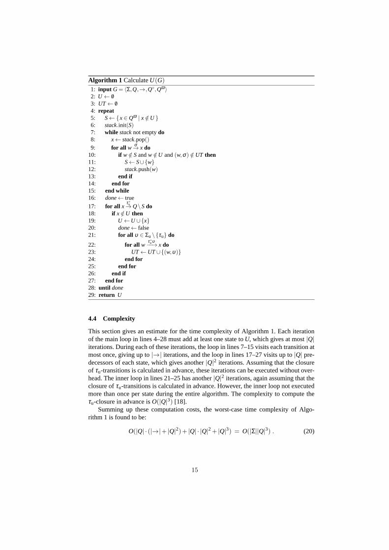
Algorithm 1 is an implementation of the iterations in Def. 13and 14 to compute theset of certainly unsupervisable states for a given automaton G. First, the sets of certainlyunsupervisable statesU and certainly unsupervisable transitionsUT are initialised inlines 2 and 3. Then the loop in lines 4–28 performs the iterations forUk(G).

The first step is to compute the supervisable statesSk+1(G), which are stored inS.In line 5, this variable is initialised to the setSk+1

0 (G) containing the accepting statesthat are not yet known to be unsupervisable. Then the loop in lines 7–15 uses astacktoperform a backwards search over the transition relation, avoiding known unsupervisablesource states and known unsupervisable transitions. Upon termination, the variableScontains the setSk+1(G) of supervisable state for the next level.

Then the loop in lines 17–27 updates the setsU andUT. For every state that was notadded toS, it explores the predecessor states reachable by sequencesof τu-transitions,and adds any states found toU, if not yet included. By adding theτu-predecessors to thesetU immediately, the reachability tests in (17) and (18) can be replaced by the directmembership tests in line 10. Next, for any new unsupervisable statex, the loop in lines21–25, searches for possible uncontrollable transitions followed by sequences ofτu andadds such combinations of source states and uncontrollableevents to the set certainlyunsupervisable transitionsUT.

The algorithm terminates if no new unsupervisable states are found during executionof the loop in lines 17–27, in which case the flagdoneretains its true value. At this point,the setU contains all certainly unsupervisable states.

14

Algorithm 1 CalculateU(G)

1: input G= 〈Σ,Q,→,Q◦,Qω 〉2: U ← /03: UT← /04: repeat5: S←{x∈Qω | x /∈U }6: stack.init(S)7: while stacknot emptydo8: x← stack.pop()

9: for all wσ→ x do

10: if w /∈ Sandw /∈U and(w,σ) /∈ UT then11: S← S∪{w}12: stack.push(w)13: end if14: end for15: end while16: done← true

17: for all xτ∗u→Q\Sdo

18: if x /∈U then19: U ←U ∪{x}20: done← false21: for all υ ∈ Σu \{τu} do

22: for all wτ∗u υ−−→ x do

23: UT← UT∪{(w,υ)}24: end for25: end for26: end if27: end for28: until done29: return U

4.4 Complexity

This section gives an estimate for the time complexity of Algorithm 1. Each iterationof the main loop in lines 4–28 must add at least one state toU, which gives at most|Q|iterations. During each of these iterations, the loop in lines 7–15 visits each transition atmost once, giving up to|→| iterations, and the loop in lines 17–27 visits up to|Q| pre-decessors of each state, which gives another|Q|2 iterations. Assuming that the closureof τu-transitions is calculated in advance, these iterations can be executed without over-head. The inner loop in lines 21–25 has another|Q|2 iterations, again assuming that theclosure ofτu-transitions is calculated in advance. However, the inner loop not executedmore than once per state during the entire algorithm. The complexity to compute theτu-closure in advance isO(|Q|3) [18].

Summing up these computation costs, the worst-case time complexity of Algo-rithm 1 is found to be:

O(|Q| · (|→|+ |Q|2)+ |Q| · |Q|2+ |Q|3) = O(|Σ||Q|3) . (20)

15

Thus, the set of certainly unsupervisable states can be computed in polynomial time.This is surprising given the nondeterministic nature of similar problems, which requiresubset construction[12]. For example, theset of certain conflicts[14], which is theequivalent of the set of certainly unsupervisable states innonblocking verification, canonly be computed in exponential time. In synthesis, the assumption of a supervisor withthe capability of full observation of the plant makes it possible to distinguish states andavoid subset construction.

4.5 Halfway Synthesis

This section introduceshalfway synthesis[9], which has been used previously [9, 16]to remove unsupervisable states in compositional synthesis, and compares it with theset of certainly unsupervisable states. It is shown that in general more states can beremoved by taking certain unsupervisability into account.

Definition 15. Let G= 〈Σ,Q,→,Q◦,Qω〉, and letΘG,τu be the greatest fixpoint of thesynthesis step operator according to Def. 8, but computed under the assumption thatΣu = {τu}. Thehalfway synthesis resultfor G is hsupC(G) = 〈Σ,Q,→hsup,Q

◦∩ ΘG,τu,

Qω ∩ ΘG,τu〉, where

→hsup= {(x,σ ,y) ∈→ | x,y∈ ΘG,τu }∪ (21)

{(x,υ ,y) ∈→ | x∈ ΘG,τu, υ ∈ Σu\{τu}, andy /∈ ΘG,τu } (22)

The idea of halfway synthesis is to use standard synthesis, but treating only thesilent uncontrollable eventτu as uncontrollable. All other events are assumed to be con-trollable, because other plant components may yet disable shared uncontrollable events,so it is not guaranteed that these events cause controllability problems [9]. After com-puting the synthesis fixpointΘG,τu, the abstraction is obtained by removing controllabletransitions to states not contained inΘG,τu, while uncontrollable transitions are retainedfor the same reasons as in Def. 12.

Theorem 6. Let G be an automaton. Then unsupC(G)⊆ hsupC(G).

Example 8. When applied to automatonH1 ‖B1 in Fig. 4, halfway synthesis removesthe crossed out states and produces the same result as unsupervisability removal. How-ever, it only considers states⊥1,⊥2, and⊥3 of W in Fig. 4 as unsupervisable, becausethe shared uncontrollable event !output1 is treated as a controllable event. This automa-ton is left unchanged by halfway synthesis.

Halfway synthesis only removes those unsupervisable states that can reach a block-ing state via local uncontrollableτu-transitions, but it does not take into account cer-tainly unsupervisable transitions. Theorem 6 confirms thatunsupervisability removalachieves all the simplification achieved by halfway synthesis, and Example 8 showsthat there are cases where unsupervisability removal can domore. On the other hand,the complexity of halfway synthesis is the same as for standard synthesis,O(|Σ||Q|3),which is the same as found above for certain unsupervisability (20).

16

5 Conclusions

The set ofcertainly unsupervisable statesof an automaton comprises all the states thatmust be avoided during synthesis of a controllable and nonblocking supervisor, in everypossible context. In compositional synthesis, the removalof certainly unsupervisablestates gives rise to a better abstraction than the previously used halfway synthesis, whilemaintaining the same cubic complexity.

The results of this paper are not intended to be used in isolation. In future work, theauthors will integrate the removal of certainly unsupervisable states with their composi-tional synthesis framework [16]. It will be investigated inwhat order to apply unsuper-visability removal and other abstraction methods, and how to group automata togetherfor best performance.

Certainly unsupervisable states are also of crucial importance to determine whethertwo states of an automaton can be treated as equivalent for synthesis purposes. Theresults of this paper can be extended to develop abstractionmethods that identify andmerge equivalent states in compositional synthesis.

References

1. de Alfaro, L., Henzinger, T.A.: Interface automata. In: Proc. 9th ACM SIGSOFT Int. Symp.on Foundations of Software Engineering 2001. pp. 109–120. Vienna,Austria (2001)

2. Asarin, E., Maler, O., Pnueli, A.: Symbolic controller synthesis for discrete and timed sys-tems. In: Hybrid Systems II, LNCS, vol. 999, pp. 1–20. Springer (1995)

3. Aziz, A., Singhal, V., Swamy, G.M., Brayton, R.K.: Minimizing interacting finite state ma-chines: A compositional approach to language containment. In: Proc. Int. Conf. ComputerDesign (1994)

4. Baier, C., Katoen, J.P.: Principles of Model Checking. MIT Press(2008)5. Baier, C., Klein, J., Kluppelholz, S.: A compositional framework for controller synthesis. In:

Katoen, J.P., Konig, B. (eds.) Proc. 22nd Int. Conf. Concurrency Theory, CONCUR 2011.LNCS, vol. 6901, pp. 512–527. Springer, Aachen, Germany (Sep 2011)

6. Fabian, M.: On Object Oriented Nondeterministic Supervisory Control.Ph.D. thesis,Chalmers University of Technology, Goteborg, Sweden (1995),https://publications.lib.chalmers.se/cpl/record/index.xsql?pubid=1126

7. Filiot, E., Jin, N., Raskin, J.F.: Compositional algorithms for LTL synthesis. In: Chin, W.N.(ed.) Proc. 8th Int. Symp. Automated Technology for Verification and Analysis, ATVA 2010.LNCS, vol. 6252, pp. 112–127. Springer, Singapore, Singapore (Sep 2010)

8. Flordal, H., Malik, R.: Compositional verification in supervisory control. SIAM J. Controland Optimization 48(3), 1914–1938 (2009)

9. Flordal, H., Malik, R., Fabian, M.,Akesson, K.: Compositional synthesis of maximally per-missive supervisors using supervision equivalence. Discrete EventDyn. Syst. 17(4), 475–504(2007)

10. Gohari, P., Wonham, W.M.: On the complexity of supervisory control design in the RWframework. IEEE Trans. Syst., Man, Cybern. (Aug 2000)

11. Hoare, C.A.R.: Communicating Sequential Processes. Prentice-Hall (1985)12. Hopcroft, J.E., Motwani, R., Ullman, J.D.: Introduction to AutomataTheory, Languages, and

Computation. Addison-Wesley (2001)13. Lin, F., Wonham, W.M.: Decentralized control and coordination ofdiscrete-event systems

with partial observation. IEEE Trans. Autom. Control 35(12), 1330–1337 (Dec 1990)

17

14. Malik, R.: The language of certain conflicts of a nondeterministic process. Working Paper05/2010, Dept. of Computer Science, University of Waikato, Hamilton, New Zealand (2010)

15. Malik, R., Streader, D., Reeves, S.: Conflicts and fair testing. Int.J. Found. Comput. Sci.17(4), 797–813 (2006)

16. Mohajerani, S., Malik, R., Fabian, M.: A framework for compositional synthesis of modularnonblocking supervisors. IEEE Trans. Autom. Control (Jan 2014),to appear

17. Mooij, A.J., Stahl, C., Voorhoeve, M.: Relating fair testing and accordance for service re-placeability. J. Logic and Algebraic Programming 79(3–5), 233–244 (Apr–Jul 2010)

18. Nuutila, E.: Efficient Transitive Closure Compuation in Large Digraphs, Acta PolytechnicaScandinavica, Mathematics and Computing in Engineering Series, vol. 74.Finnish Academyof Technology, Helsinki, Finland (1995)

19. Pnueli, A., Rosner, R.: On the synthesis of a reactive module. In:Proc. 16th ACM Symp.Principles of Programming Languages. pp. 179–190 (1989)

20. Wonham, W.M.: On the control of discrete-event systems. In: Nijmeijer, H., Schumacher,J.M. (eds.) Three Decades of Mathematical System Theory. LNCIS,vol. 135, pp. 542–562.Springer (1989)

18

Wind Turbine System : An Industrial Case Study inFormal Modeling and Verification

Jagadish Suryadevara1, Gaetana Sapienza2,Cristina Seceleanu1, Tiberiu Seceleanu2, Stein-Erik Ellevseth2, and Paul Pettersson1

1 Malardalen Real-Time Research Centre, Malardalen University, Vasteras, Sweden.{jagadish.suryadevara,cristina.seceleanu,paul.pettersson}@mdh.se

2 ABB Corporate Research.{gaetana.sapienza,tiberiu.seceleanu}@se.abb.com,

stein-erik.ellevseth@no.abb.com

Abstract. In the development of embedded systems, the formal analysis of sys-tem artifacts, such as structural and behavioral models, helps the system engi-neers to understand the overall functional and timing behavior of the system. Inthis case study paper, we present our experience in applying formal verificationand validation (V&V) techniques, we had earlier proposed, for an industrial windturbine system (WTS). We demonstrate the complementary benefits of formalverification in the context of existing V&V practices largely based on simulationand testing. We also discuss some modeling trade-offs and challenges we haveidentified with the case-study, which are worth being emphasized. One issue isrelated, for instance, to the expressiveness of the system artifacts, in view of theknown limitations of rigorous verification, e.g. model-checking, of industrial sys-tems.

Keywords: Industrial Case-Study, Wind Turbine System, MARTE/CCSL,EAST-ADL, Verification, Model Checking, UPPAAL

1 Introduction

The increasing complexity and criticality of real-time embedded systems (RTES), indomains such as industrial automation, automotive and avionics, stresses the need forapplying systematic design phases, combined with rigorous verification and valida-tion (V&V) techniques, during system development [3]. A well-defined design processwith necessary tool support leads to ensuring system predictability, w.r.t intended func-tional and timing behavior. Nevertheless, meeting such a clear objective has severalchallenges. One of pre-requisites is well-defined system artifacts representing systemstructure as well as behavior with reactive, continuous, discrete, and real-time fea-tures, or a combination thereof, at suitable levels-of-abstraction. For complex industrialsystems, the above design by-products, while necessary, may lead to additional issuessuch as ensuring traceability, analyzability as well as reusability of the system artifacts.In this context, model-based development approaches, which enable continuous V&Vthroughout the development process, have become a feasible solution to tackle some ofthe challenges. However, formal verification techniques such as model checking, while

19

useful for the exhaustive analysis of system behavior, are challenging to apply for com-plex system models. A related issue is choosing a suitable level of granularity and ex-pressiveness for system artifacts, given the well-known limitations of model-checking,such as the state-space explosion problem. In this paper, we address some of these chal-lenges in the context of applying modeling and formal verification techniques using awind turbine system case-study, a complex industrial RTES.

The Unified Modeling Language (UML) provides a modeling profile calledMARTE (Modeling and Analysis of Real-Time and Embedded systems) [7] to supportthe performance and schedulability analysis of system models. MARTE also includesCCSL – a time model and a clock constraint specification language [1] for specifyinglogical and chronometric constraints for system models. On the other hand, EAST-ADL[2], an emerging standard for automotive systems, provides an integrated model-baseddevelopment for RTES, through well-defined phases, as well as support for traceability.Recently, EAST-ADL has been integrated with model-checking support for component-based designs, e.g. the ViTAL tool [4] based on the timed automata technology forverification [5,11,10].

In this paper, we target the verification of functionality and timing behavior of awind turbine system developed in the context of the iFEST (industrial Framework forEmbedded Systems Tools), an ARTEMISIA project. In Section 2.2, we overview asimplified version of the wind turbine system (WTS), and describe its functionality andtiming behavior. Rest of the paper is organized as follows: In Section 3, we briefly recallCCSL and timed automata. In Section 4, we describe a modeling methodology for theWTS to enable verification using model checking. The analysis results of simulating,as well as model checking the WTS model are presented in Section 5. In Section 6, wediscuss our experience with the case study with respect to the challenges and limitationsin applying formal techniques to complex industrial systems. We conclude the paper inSection 7.

2 Windturbine System (WTS) : An overview

Wind energy sources are fast-growing and in line with the technological advancement.Modern wind turbine systems require sophisticated and effective control functionalitiesin order to fulfill performance, safety, and maintainability requirements. The main pur-pose of a wind turbine system is to convert the rotational mechanical energy of the rotorblades (i.e. mechanical components of a wind turbine) caused by the wind into electri-cal energy to be redistributed via a power grid. Given the system’s complexity, theiFEST (industrial Framework for Embedded Systems Tools) project3 aims at providinga model-based approach for system development, to ensure the system predictabilityw.r.t the specified functional and timing behavior.

2.1 Development Process and Environment

In the iFEST project, we have carried out the system development by adopting the V-model based software development approach, as follows:

3 http://www.artemis-ifest.eu/

20

During Requirement and Analysis phase, we have documented the WTS require-ments, both functional and extra-functional including timing behavior. For the Designphase, we have combined component- and model-based approaches, keeping in viewthe overall system analyzability and reusability requirements. During the Implementa-tion phase, we have applied automatic code generation technologies.Subsequently, theimplemented system, a combined FPGA and CPU solution, has been deployed on a het-erogenous hardware platform (XilinX ZynQ 7000 product family). For the Verificationand Validation (V&V), we have used model-based techniques as follows: (i) simula-tion of the WTS functionality using Simulink and related toolboxes, and (ii) automaticmodel-based test-case generation with MaTeLo tool. However, the above techniquesare not sufficient to ensure system predictability w.r.t to all possible system executions,hence formal verification is desirable to complement the current analysis methods. Toaddress the above open issue, in this paper, we present a verification technique towardsenhanced system validation. And, our contributions are as below:

– As enhanced system validation, we apply verification technique to establish sys-tem properties, (partially) based on simulation results of Simulink-based systemmodels.

– We are able to verify safety requirements that involve timing behavior (e.g. “thewind turbine moves to Park mode, within 30s of detecting that the wind speed hascrossed the upper limit of 20m/sec”).

2.2 The Wind Turbine System Model

The wind turbine system is modeled as a closed-loop control system, as shown in Fig-ure 1. The key components are the Plant and the Controller subsystems. The Controllerdynamically regulates the rotor blades of the wind turbine w.r.t the specified wind pro-file, to maximize the generation of electrical energy and also to avoid damage to theplant in case of turbulent wind scenarios. It automatically changes the Controller Out-put signal to regulate the plant, based on the wind and the plant’s actual conditions,which are received by the Controller via the Sensor Input signals. The Wind Profileand the Resistive Load are used to simulate and test the behavior of the plant and thecontroller, under specific wind and resistive load conditions. Further details of the plantand controller subsystems are described below.

2.2.1 Plant model. As shown in Figure 2 (in Section 4), it consists of three maincomponents; Servo, Rotor, and Generator. The pitch of the turbine, determined by theController (described below), is actuated by the Servo. The Rotor produces the requiredtorque to maximize the angular speed of the Generator (which produces the final volt-age), based on the pitch value as well as the current wind speed (we assume a fixedresistive load). The Rotor optimizes the produced torque value based on the currentangular speed of the Generator.

2.2.2 Controller model. As shown in Figure 3 (in Section 4), it consists of fourmain components: the Filter, the Main Controller, the Pitch Controller, and the Park

21

Fig. 1. Wind Turbine System Model

and Brake Controller. The Filter Subsystem is responsible for transducing, filteringand scaling the wind signal and plant signal (for instance the rotational speed of theturbine), which are used by the Main Controller and the Pitch Controller. Based on theinputs received through the Filter, the Main Controller directs the overall control. Itoversees the performance and operations of the turbine in order to maximize the energyproduction and prevent any damage to the plant. Based on the wind and plant state, thecontroller determines the operational mode (i.e. park, start-up, generating, or brake) ofthe turbine. The Pitch Control calculates the proper pitch i.e. angle to steer the rotorblades when the turbine starts up or generates power. The Pitch and Brake controllerdetermines if the turbine needs to brake or park, to ensure the safety of the wind turbine,for instance, during wind turbulances.

3 Preliminaries

In this section, we present an overview of the preliminaries needed for modeling ofthe wind turbine system. We have used EAST-ADL modeling framework for structuralmodeling of the WTS. The timed causality behavior of the system is specified usingCCSL. To provide the verification using the UPPAAL, a model checking tool, we havedeveloped the timed automata based semantic models of the system, based on the cor-responding EAST-ADL models and the CCSL specifications.

3.1 EAST-ADL

The modeling process in EAST-ADL framework, developed in the context of the EAST-EEA project, is structured into different abstraction levels such as feature level, anal-ysis level, design level etc. At both analysis and design levels, the system is describedby a FunctionalArchitecture that consists of a number of inter-connected FunctionPro-totypes (instantiation of FunctionType components). FunctionProtoype components areeither event- or time-triggered. The execution semantics of the EAST-ADL componentsis as follows; components interact through single buffer, rewritable, non-consumableports, and execute in read-execute-write phases in run-to-completion fashion. The de-tailed timing behavior as well as timing constraints for an EAST-ADL model can bespecified using TADL2, the Timing Augmented Description Language (ver 2), cur-rently being integrated with EAST-ADL framework [8]. In related works, we have pro-posed verification techniques for TADL2-based EAST-ADL models [5,11,10].

22

3.2 CCSL

CCSL is used to specify the constraints imposed on the logical clocks (activation con-ditions) of a model. A CCSL clock is defined as a sequence of instants (event occur-rences). CCSL constraints are of three kinds: (i) Synchronous constraints rely on thenotion of coincidence. For example, the constraint “a coincidesWith b”, denotedby a = b, specifies that each instant of a coincides with the corresponding instant ofb. Another example of a synchronous constraint is “a isPeriodicOn b periodn” , which specifies the subclock a whose ‘ticks’ correspond to every nth ‘tick’ ofb. (ii) Asynchronous constraints are based on instant precedence; the constraint “aisFasterThan b” (denoted by a 4 b) specifies that clock a is (non-strictly)faster than clock b. (iii) Mixed constraints combine coincidence and precedence; theconstraint “c = a delayedFor n on b” specifies that c ‘ticks’ synchronously withthe nth ‘tick’ of b following a ‘tick’.

3.3 Timed Automata

A timed automaton is a tuple < L, l0, C,A,E, I >, where L is a set of locations,l0 ∈ L is the initial location, C is the set of clocks, A is the set of actions, synchroniza-tion actions and the internal τ -action, E ⊆ L× A× B(C)× 2C × L is a set of edgesbetween locations with an action, a guard, a set of clocks to be reset, and I : L→ B(C)assigns clock invariants to locations. A location can be marked urgent (u) or commit-ted (c) to indicate that the time is not allowed to progress in the specified location(s), thelatter being a stricter form indicating further that the next transition can only be takenfrom the corresponding location(s) only. Also, synchronization between two automatais modeled via channels (e.g., x! and x?) with rendezvous or broadcast semantics.

The UPPAAL model-checker extends the timed automata language with a numberof features such as global and local (bounded) integer variables, arithmetic operations,arrays, and a C-like programming language. The tool consists of three parts: a graphicaleditor for modeling timed automata, a simulator for trace generation, and a verifier forthe verification of a system modeled as a network of timed automata. A subset of CTL(computation tree logic) is used as the input language for the verifier. For further details,we refer to UPPAAL tutorial [6].

4 WTS: Formal Specification and Modeling

In this section, we present a formal specification and modeling approach for WTS,an aposteriori modeling technique, that is, the specification and modeling artifacts arebased on existing design artifacts such as Simulink models, requirements documentsetc. However, we apply an abstraction strategy to obtain the corresponding real-timesemantic models that represent the system functionality as well as the timing behav-ior. Further, the strategy attempts to preserve the models’ tractability to make the ex-haustive verification feasible. The overall modeling strategy, based on design principlessuch as separation-of-concerns and correctness-by-construction, captures the underly-ing model-of-computation and the execution behavior of the WTS. Below, we outlinesome generic views/assumptions on which we base our formal modeling:

23

– Plant models and Instantaneous executions. A Plant model represents phys-ical devices such as sensors and actuators with the corresponding model-of-computation based on reactivity and instantaneity.

– Controller models and Timed executions. Controllers contain software compo-nents based on timed model-of-computation, with explicit timing aspects, such asdelay, execution time, end-to-end deadline etc, to be formally specified and mod-eled.

– Time and event triggering. The activation or triggering of RTES components isgenerally based on specific time or event4 occurrences. Plant components are event-triggered (i.e. in response to occurrence of input data), whereas controller compo-nents are time- or event-triggered, this primarily being a design-choice.

– Run-to-completion. RTES components execute in run-to-completion steps, that is,in terms of read-execute-write cycles.

– Data and value semantics. Due to the associated models-of-computation, as de-scribed above, a data entity at a given ‘instant’, in the Plant or Controller, maycorrespond to two distinct value instants.

– Real-time features. The structural and behavioral models of RTES often fail tomodel real-time features, such as urgency, priority, and synchrony (explained later)w.r.t to the underlying execution model.

– Environment modeling. An environment is external to the system, representingphysical parameters such as temperature, pressure, wind speed etc. To support for-mal verification, a modeling strategy based on non-determinism as well as the prop-erties to be verified, is needed.

To obtain an expressive and verifiable semantic model of the WTS, we employ acomponent-based modeling approach, based on real-time formalisms such as CCSLand timed automata.The overall modeling approach is as follows:

– Data and event representations are made based on the structural models.– The timed causality behavior of the system components, w.r.t the associated model-

of-computation, is formally specified using CCSL constraints.– The functional behavior of the components is modeled using an abstract finite-state-

machine notation, and transformed into timed automata.– The CCSL constraints are transformed into timed automata, and composed using

the notion of synchronization product (described later).

Finally, a real-time semantic model of the overall system is obtained as a network (i.e.,a parallel composition) of timed automata described above.

Fig. 2. Structural modeling: a plant model for the WTS.

4 While time is also an ‘event’, we differentiate this in this paper explicitly.

24

In Figure 2, we present the structural model of plant and controller for the WTS(based on the corresponding Simulink models), using the EAST-ADL modelingframework (in MetaEdit+5). The main components of the plant, that is SERVO,ROTOR, and GENERATOR are modeled as FunctionalDevice prototypes inEAST-ADL. In Figure 3, we present the structural model of the Controller. It modelsthe three sub-controllers MainControl, PitchRegulation, and ParkBrake, modeledas AnalysisFunctionTypes. For further details of the functionality of thesecomponents, we refer to Section 2.2. We demonstrate the overall modeling approachfor WTS, using the ROTOR and the MainControl components, below. We will alsodiscuss some related modeling issues.

Fig. 3. Structural modeling: a controller model of the WTS.

4.1 Data and Events

As shown in Figure 2, the ROTOR prototype, denoted by RT, receives input pitch(theta), turbine speed (omega), and wind speed (ws) and produces the correspond-ing torque value as the output. Hence, we define the local variables thetal, omegal,and wsl and the corresponding global variables wsg , omegag , thetag . The local vari-ables are updated at the activation of the RT using the corresponding global values. Thisis consistent with the data semantics discussed previously.

1 CCSLclock RT in ; / / r e a d ( i n p u t ) i n s t a n t sCCSLclock RT out ; / / w r i t e ( o u t p u t ) i n s t a n t s

3 CCSLclock RT omega ; / / a c t i v a t i o n ( t r i g g e r ) i n s t a n t s

5 C C S L c o n s t r a i n tRT omega = RT in ; / / RT omega coincidesWith RT in

7 RT in = RT out ; / / RT in coincidesWith RT out

Listing 1.1. CCSL specification of ROTOR component.

4.2 Specification of timed causality behavior

The timed causality behavior of real-time components, w.r.t the correspondingmodel-of-computation, can be specified precisely using CCSL logical clocks andCCSL constraints. We use CCSL (logical) clocks to represent events correspondingto ‘read’, ‘execute’, and ‘write’ instants of a component. In Listing 1.1 and Listing1.2, we present the CCSL specification of ROTOR (RT) and MainControl (MC)

5 www.metacase.com

25

Table 1. Timing attributes of Controller components.

Min MaxComponent Period Execution Time Execution Time

(ms) (ms) (ms)

MainControl 100 10 15PitchRegulation 50 35 45ParkBrake 50 15 20Filter – 20 25

prototypes, respectively. The constraints specify the timed causality behavior of thecomponents w.r.t to the corresponding model-of-computation. For instance, the CCSLconstraints for RT specify the reactivity and instantaneity behavior of RT executionwithin the Plant model. On the other hand, the CCSL constraints for MC specifythe time-triggered behavior of the controller execution. The timing attributes of thecontroller components are given in Table 1. The CCSL specifications provide a basisfor constructing real-time semantic models e.g. timed automata based models, as wellas observers to establish the system properties, as presented later in this section.

1 CCSLclock MC in / / r e a d ( i n p u t ) i n s t a n t sCCSLclock MC out / / w r i t e ( o u t p u t ) i n s t a n t s

3

C C S L c o n s t r a i n t

5 MC in delayedFor 10 on SysClk 4 MC out / / Minimum e x e c u t i o n t i me

MC out 4 MC in delayedFor 15 on SysClk / / Maximum e x e c u t i o n t i me7 MC in isPeriodicWith period 100 on SysClk / / Time t r i g g e r i n g

Listing 1.2. CCSL specification of MainControl component.

4.3 Modeling functional behavior of real-time components

In Figure 4, we present the behavior modeling for the MainControl protoype (basedon the corresponding Simulink model). The behavior is specified using a finite-state-machine (FSM) notation. It represents the overall system behavior (stateful) in termsof control states PARK, START, BRAKE, and GENERATE. The states represent theoperational modes of the WTS, based on the wind speed and the turbine speed; themode transitions corresponding to mode-change behavior are triggered by booleanconditions (guards) g1, g2, .. etc. Further, we simply annotate the behavior model todenote the execution semantics such as run-to-completion (R-T-C) and history (denotedby the control node H). The functionality of other components in the WTS are statelesscomputations, that is partial functions between input and corresponding output values,for instance as represented by the writeTorque() function of the ROTOR.

4.4 Formal modeling of Plant components

In this subsection, we present formal modeling approach, based on CCSL, for theplant components of the WTS. We had earlier proposed, in a previous work [10],

26

Park

Start

Brake

Generate[g1] [g5]

[g3]

[g2] [g4]

[g6]

H

R-T-C

Fig. 4. Functional behavior of the MainControl component.

transformation of CCSL constraints into timed automata. The transformations can beused to derive timed automata based models that represent the timed causality behaviorof the system. For instance, in Figure 5.(a) and 5.(b), we present the timed automatasemantics of CCSL constraints that specify the timed causality behavior of ROTORexecutions (see Listing 1.1), using events RT in and RT out representing componentactivation and termination respectively. Note that an event e.g. RT in is modeledusing synchronization channels i.e. send/receive signals RT in! and RT out!. Alsonote that the synchronous occurrence of event signals, e.g. GR out? and RT in! inFigure 5.(a), is specified using committed locations. A committed location indicatesthat the corresponding enabled transitions from the location are ‘forced’ before timecan progress. This facilitates precise modeling of overall timing behavior of the system.

(b) (c)(a)

Fig. 5. Timed automata modeling: (a) RT omega = RT in (b) RT in = RT out (c)Computation RT.

The above automata can be composed, using the notion of synchronization product(based on common labels or synchronization signals), as shown in Figure 6.(a). Forinstance, locations B and C in the automata in Figure 5.(a) and Figure 5.(b) respectively,are mapped to the location BC in Figure 6.(a), due to the synchronization of signalsRT in! and RT in?.

(a) (b)

Fig. 6. Timed automata model for (event-triggered) ROTOR.

It can be noted that the composed location ‘BD’ is not possible in the synchronizedproduct automaton, as the location is non-reachable due to the synchronization atB and C, leading to location AD (i.e. location A, and D simultaneously in resp.automata) in the synchronized product, instead. Further, as shown in Figure 6.(a), we

27

associate the transitions corresponding to component activation, with data updates andthe corresponding computation; the RT in event denotes input as well as executionof the corresponding functionality, during a transition from location BC to locationAD. However, to make the overall automata model of the WTS system tractable(time-wise), and hence formally verifiable, we need to relax the notion of instantaneityfor the automata models of the Plant components. This can be done by introducinga minimum time delay for each component, if not specified already. This is done byassigning a timing invariant, the delay of one time unit, for instance at location AD inFig.6.(b).

(a) (b) (c)

Fig. 7. Semantic modeling: (a) Periodic triggering (b) Min. exec. time (c) Max. exec. time

4.5 Formal modeling of Controller components

In this subsection, we describe the timed automata modeling of the Controllercomponents for the WTS. In Figure. 7, we present the timed automata semantics ofthe CCSL constraints (Listing 1.2) that specify the time-triggered execution behaviorof the MainControl (MC) prototype. We have composed these automata, as shownin Figure 8.(a), based on the notion of synchronization product (as described in theprevious subsection). This consists of following steps; we have composed the automatain Figure 7.(b) and 7.(c), and then finally with the automaton in Figure 7.(a) (note theinvariant y ≤ 100 at every location in the product automaton).

(a) (b)

Fig. 8. Timed automata modeling of MainControl: (a) time-triggering (b) functional behavior.

As shown in Fig.8.(b), we have also transformed the behavior (functional) modelof the MainControl (Fig.4) component into corresponding timed automaton, followingthe mapping techniques proposed previously [9]. We briefly outline the transformationas follows; we have mapped the control states to automaton locations. Further, usingadditional locations Init and Final and the history variable ‘h’, we have modeled theexecution semantics, that is, run-to-completion, and preserving the history. For model

28

readability, we have not shown the data updates for the transitions; also, the booleanguards of the form ‘eij’ correspond to actual expression (¬gi && ¬gj). It can benoted that all the locations of the transformed automaton are marked ’urgent’ indicat-ing the behavior model does not consume time, which has been separately modeledusing the timed causality model discussed above. Finally, we ‘connect’ the transformedbehavior model of the MainControl prototype, as described above, with the automatamodel of the corresponding timing behavior (Fig.8.(b)), using synchronization channel‘execute’.

4.6 Modeling the WTS system

Following the modeling strategy presented in the previous subsections, we can obtainthe timed automata models for all the WTS components, and form a network (parallelcomposition) of these automata to obtain a timed automata based semantic model forthe complete system. However, some issues exist as discussed below:

Modeling the Environment: The plant model described previously, models the com-ponents such as sensors and actuators constituting an environment model for the WTScontroller. However, this is not sufficient to obtain a ‘closed’ model of the system that isnecessary to enable exhaustive verification of the WTS model. For instance, modelingexternal parameters such as WindSpeed, while necessary, is not feasible using timedautomata. In view of this, as well as the hybrid nature of the plant components e.g. RO-TOR, GENERATOR etc, we choose to integrate the simulation data of the correspond-ing Simulink models, to construct the partial functions that represent the computationsof the components.

Modeling ‘observer’ automata: The formal specification of complex properties of thesystem, while possible using CTL (the property specification formalism of UPPAAL),may not be directly verifiable. Instead, these can be intuitively modeled as observerautomata, (parallel) composed with the main system model, and can be efficiently ver-ified.

5 WTS Analysis

In this section, we present both simulation as well as the verification results for theWTS, and their correlation in verifying functional and safety-critical properties w.r.tthe overall timing behavior of the system.

5.1 Simulation

The main purpose of simulating the WTS, using the MathWorks Simulink andStateFlow6, is to analyze the system behavior under normal operating conditions, andto validate the system (in particular the Controller) when the wind speed exceeds the

29

0 10 20 30 40 50 60 70 800

2040

Wind Speed

m/s

ec

0 10 20 30 40 50 60 70 80-202

Rotor Torque

Nm

0 10 20 30 40 50 60 70 800

2040

Rotor Speedra

d/s

ec

0 10 20 30 40 50 60 70 80-100

0100

Servo Motor Angle

Deg

0 10 20 30 40 50 60 70 80-100

0100

Pitch

Deg

0 10 20 30 40 50 60 70 80024

Turbine State

Time (sec)

Sta

te

Fig. 9. Simulation Results

designed limit. The simulation results are presented in Figure 9.

The simulation time is step-wise incremented from 0 up to 80 sec., with a fixedsample time equal to 1 msec. For the simulation, a specific wind speed profile has beencreated. According to this, the system is simulated for normal operating limits, i.e., 5- 20 m/sec up to 30 sec, then up to 30m/sec above 43 sec. The simulation results areanalyzed w.r.t the turbine control states representing the operational modes (i.e. 0:park,1:start, 2:generate, 3:brake).

While the simulation provides rich data representing the computation and controlof the WTS w.r.t complex environment behavior, system properties however can not beestablished without analyzing the data. In the next subsection, we present a verificationtechnique to ‘exhaustively’ analyze the simulation data, w.r.t the overall system timingand causality behavior, towards establishing the system properties. Below, we describesome verification results for the WTS system.

5.2 Verification

For WTS, a formal modeling of the corresponding plant and the environment param-eters is not possible. Hence, we use simulation data and construct partial functions(input to output values) that represent the computations of the plant components, forinstance ROTOR. Also, we use simulation values corresponding to the environmentparameters e.g. wind-profile of the WTS. In the next section, we will discuss someaspects about the construction of the relevant partial functions.

Verification of functional properties: Verification of functional properties gives insightinto the overall system (architectural) design. For instance, in the WTS case, it is usefulto verify the following property: “if the wind speed is within the prescribed limits, the

6 http://www.mathworks.se/products/stateflow/

30

controller eventually moves to Generate mode”. The property can be formulated asa liveness property or leads to property (denoted by , implemented as --> inUPPAAL), as below.

(ws>=5 && ws<=20) --> state==2 (1)

Verification of safety-critical properties: One of the safety-critical requirements for theWTS is to fulfill the following property: “the wind turbine moves to Parkmode, within30s from detecting that the wind speed has crossed the upper limit of 20m/sec”. Toverify the property (w.r.t to simulation data), we construct an observer automata for theproperty as shown in Fig.10, compose the observer with the system model, and verifythat the corresponding invariant, the Property (2), holds for the composed model. Notethat the urgent channel ‘U!’ forces the transition from location B to A without anyfurther delay, when the corresponding transition is enabled.

A� obs.B implies x <= 30 (2)

x=0

x=0 BA

U!state==3

ws>20

Fig. 10. An observer automata to verify the safety-property: A[] obs.B implies x<=30

Verifying reachability properties: We can verify reachability of specific control statesor computation. For instance, using the Property 3, a reachability property, we canverify that the control state ‘Park’ (Figure 8.(b)) has been reached (at least once) duringthe simulation of the WTS. While this may be easily validated using the simulationtrace, we can use similar properties to verify specific ‘error’ states e.g. by extendingthe behavior model with special ‘locations’ that are reached if the corresponding ‘error’is detected. The presence of these error locations in the simulation data can then be‘exhaustively’ verified.

∃ <> MC.Park (3)

Verifying deadlock-freeness: Using the Property 4, we can verify that the system isdeadlock-free, w.r.t overall timed causality behavior of the WTS, as modeled by thecorresponding timed automata model. The property is an important validation of thesystem, which can not be achieved using simulation only, as the corresponding Simulinkmodel does not represent the timing behavior of the system explicitly. Also, the prop-erty, when satisfied, verifies the correctness (i.e. consistency) of the timing attributes(Table 1) associated with the system (architectural) design.

A� (not deadlock) (4)

31

6 Discussion and Lessons-learned

In this paper, we have presented a formal modeling and verification approach for anindustrial system, namely a wind turbine system. The main goal of the work has been toprovide formal verification as a complementary analysis method to existing validationtechniques based primarily on simulation. We have successfully addressed the follow-ing challenges:

– Abstract but expressive system models: Using real-time formalisms such as CCSLand timed automata, we were able to construct intuitive system models amenablefor exhaustive verification (w.r.t to timing). With the separation of timing andfunctional modeling, the technique is scalable to complex system models.

– Verification as complementary analysis to simulation: The verification is based on‘exhaustively’ analyzing the simulation data w.r.t the timing behavior of the sys-tem. While verification models are expressive in terms of system structure andprecise timing behavior, simulation models are suitable to specify plant and theenvironment, e.g. ‘wind profile’ modeling in the case of WTS simulation. Thus, theverification approach provides an enhanced simulation-based validation.

The formal modeling approach for the wind turbine system considers the cor-responding simulation results to model a suitable abstraction of the plant model. Itfacilitates constructing a formal model of the WTS, including the plant behavior. Thiswas primarily one of the obstacles in earlier efforts to achieve formal verificationof the system. Besides, the formal models were only possible due to expressivenessof real-time semantic formalisms such as CCSL and modeling flexibility in timedautomata, as demonstrated in this paper. Further, we believe that the modeling approachis scalable to large complex systems, due to parallel composition of semantic models(timed automata) representing system components. For the verification results, we haveconsidered only the control properties of the system with respect to the overall timedcausality behavior. However, we can also consider the data values in the verification,due to timed automata variables. Thus, we have combined the expressiveness of CCSLwith modeling capabilities of timed automata.

However, some limitations of our approach do exist. The exhaustiveness of the veri-fication is limited to partial functions constructed using specific instance(s) of simula-tion. Hence, the approach may be similar to testing-based analysis (albeit model-based).Hence, we need strategies, e.g. choosing suitable simulation step and data profiles, togenerate simulation data w.r.t the system properties to be verified. Further, it may benoted that the simulation-extended verification approach presented above may be suit-able for data-intensive control systems (e.g. hybrid systems), such as the wind turbinesystem case study presented in the paper. On the other hand, control-intensive systemsmay be exhaustively modeled and verifiable using model-checking independent of sim-ulation.

32

7 Conclusion

In this paper, we have presented a formal modeling and verification approach for anindustrial case-study, namely an example wind turbine system. The architectural andbehavioral modeling, partially based on the existing system artifacts such as Simulink-models, additionally captures precise timing behavior of the system. The modeling ap-proach, based on the real-time formalisms such as CCSL and timed automata, alsointegrates simulation data to model plant and environment behavior. Based on this, theproposed verification technique using model-checking, enhances the simulation-basedsystem validation. Besides verifying functional properties that validate correctness ofthe system design, safety-critical properties w.r.t the overall system timing behaviorcan also be verified. This is clearly an important analysis step forward within existingvalidation approaches for industrial applications. Thus the paper addresses V&V chal-lenges in the industrial context, by combining both simulation and verification tech-niques, paving the way towards scalable application of model-checking for an enhancedvalidation process. As future work, we intend to investigate requirement-driven strate-gies to derive the simulation criteria for generating relevant partial functions. This leadsto enhanced validation process that can verify useful classes of system properties.

Acknowledgment

This work was partially funded by Swedish Research Council (project ARROWS),Malardalen University (Sweden), and ARTEMISIA project iFEST.

References

1. Andre, C., Mallet, F., de Simone, R.: Modeling Time(s). In: Models’07. LNCS, vol. 4735,pp. 559–573. Springer (2007)

2. ATESST (Advancing Traffic Efficiency through Software Technology): East-ADL2 specifi-cation (March 2008), http://www.atesst.org, 2008-03-20

3. Bouyssounouse, B., Sifakis, J.: Embedded Systems Design: The ARTIST Roadmap for Re-search and Development (Lecture Notes in Computer Science). Springer-Verlag New York,Inc., Secaucus, NJ, USA (2005)

4. Enoiu, E.P., Marinescu, R., Seceleanu, C., Pettersson, P.: Vital : A verification tool for east-adl models using uppaal port. In: ICECCS’12 (July 2012)

5. Goknil, A., Suryadevara, J., Peraldi-Frati, M.A., Mallet, F.: Analysis Support for TADL2Timing Constraints on EAST-ADL Models. In: ECSA 2013 : 7th European Conference onSoftware Architecture. p. 10 pages. LNCS, Montpellier, France (Jul 2013)

6. Larsen, K.G., Pettersson, P., Yi, W.: UPPAAL in a Nutshell. Int. Journal on Software Toolsfor Technology Transfer 1(1–2), 134–152 (Oct 1997)

7. OMG: UML Profile for MARTE, v1.0. Object Management Group (November 2009),formal/2009-11-02

8. Peraldi-Frati, M.A., Goknil, A., DeAntoni, J., Nordlander, J.: A Timing Model for SpecifyingMulti Clock Automotive Systems: The Timing Augmented Description Language V2. In:ICECCS 2012. pp. 230–239 (2012)

33

9. Slutej, D., Hakansson, J., Suryadevara, J., Seceleanu, C., Pettersson, P.: Analyzing a pattern-based model of a real-time turntable system. In: Jens Happe, B.Z. (ed.) 6th Interna-tional Workshop on Formal Engineering approaches to Software Components and Architec-tures(FESCA), ETAPS’09, York, UK, March. pp. 161–178. Electronic Notes in TheoreticalComputer Science (ENTCS), Vol 253, Elsevier (September 2009)

10. Suryadevara, J., Seceleanu, C., Mallet, F., Pettersson, P.: Verifying MARTE/CCSL modebehaviors using UPPAAL. In: 11th International Conference on Software Engineering andFormal Methods (SEFM 2013) (September 2013)

11. Suryadevara, J.: Validating EAST-ADL timing constraints using UPPAAL. In: 39th Euromi-cro Conference on Software Engineering and Advanced Applications SEAA 2013) (Septem-ber 2013)

34

Precise Documentation and Validation ofRequirements

Chen-Wei Wang, Jonathan S. Ostroff, Simon Hudon

Department of Electronic Engineering & Computer Science, York University{jackie, jonathan, simon}@cse.yorku.ca

Abstract. Precise documentation of requirements is important for de-veloping and certifying mission critical software. We specify cyber-physicalsystems via an Event-B-like machine which declares the monitored andcontrolled variables and their initial condition. A machine event modelsthe joint action of the plant and the controller. Embedded in the eventaction is a function table that specifies the input-output behaviour of thecontroller, as monitored variables are periodically updated by the plant.We extend the Event-B notation with queries and modules. The result-ing machine provides us with a mathematical description of the overallsystem behaviour, thus allowing us to validate the requirements by prov-ing that (1) the input-output specification of the controller is complete,disjoint and well-defined, and that (2) the machine satisfies system-wideconsistency invariants elicited from domain experts. A biomedical deviceis used as a case study, and we mechanize proofs via a SMT solver.

Keywords: certification, requirements documentation and validation,model contracts, well-definedness, tabular expressions

1 Introduction

The central task of system development is to design the system such that itsoverall behaviour satisfies the requirements. But this assumes that the require-ments are precise and complete, while problems in the requirements phase willnegatively impact the subsequent phases of design and implementation.

Requirements are often stated informally using natural languages, which tendto be imprecise and incomplete. It is rather difficult to reliably check that Englishnarratives, or even semi-formal models such as use cases, address all scenariosrelevant to the task at hand. Nevertheless, precise documentation of requirementsis important for validating, verifying and certifying mission critical software inmedical, automotive, nuclear and avionic systems [13].

Industrial standards such as IEEE 7-4.3.2 (nuclear), ISO 26262 (automotive)and DO-178C (avionics) recommend the use of formal methods. But formalmethods alone do not guarantee that requirements will be complete. Tabularexpressions [20] (a.k.a. function tables) describe computer controllers as math-ematical functions relating system stimuli and responses. Tabular expressionshave been adopted in the nuclear domain to ensure that specifications are com-plete and disjoint [11, 21, 22].

35

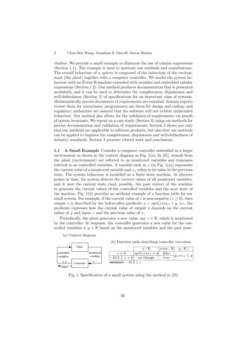
2 Chen-Wei Wang, Jonathan S. Ostroff, Simon Hudon

Outline. We provide a small example to illustrate the use of tabular expressions(Section 1.1). The example is used to motivate our methods and contributions.The overall behaviour of a system is composed of the behaviour of the environ-ment (the plant) together with a computer controller. We model the system be-haviour with an Event-B machine extended with modules and embedded tabularexpressions (Section 1.2). Our method produces documentation that is presentedmodularly, and it can be used to determine the completeness, disjointness andwell-definedness (Section 2) of specifications for an important class of systems.Mathematically precise documents of requirements are essential: domain expertsreview them for correctness; programmers use them for design and coding; andregulatory authorities are assured that the software will not exhibit unintendedbehaviour. Our method also allows for the validation of requirements via proofsof system invariants. We report on a case study (Section 3) using our methods forprecise documentation and validation of requirements. Section 3 shows not onlythat our methods are applicable to software products, but also that our methodscan be applied to improve the completeness, disjointness and well-definedness ofindustry standards. Section 4 presents related work and conclusions.

1.1 A Small Example Consider a computer controller embedded in a largerenvironment as shown in the context diagram in Fig. 1(a). In [21], stimuli fromthe plant (environment) are referred to as monitored variables and responsesreferred to as controlled variables. A variable such as z (in Fig. 1(a)) representsthe current value of a monitored variable and z-1 refers to its value in the previousstate. The system behaviour is modelled as a finite state machine. At discretepoints in time, the system detects the current values of all monitored variables,and it uses the current state (and, possibly, the past states) of the machineto generate the current values of the controlled variables and the next state ofthe machine. Fig. 1(b) provides an artificial example of a function table for oursmall system. For example, if the current value of z is non-negative (z ≥ 0), thenoutput x is described by the before-after predicate x = sqrt(z )∗x-1 + y , i.e., thepredicate expresses how the current value of output x depends on the currentvalues of y and input z and the previous value of x .

Periodically, the plant generates a new value, say z ∈ R, which is monitoredby the controller. In response, the controller generates a new value for the con-trolled variables x , y ∈ R based on the monitored variables and the past state.

(a) Context diagram

Plant

Controller zx, y

monitored variables

controlled variables

error

(b) Function table describing controller execution

x : R error : B y : R |z ≥ 0 sqrt(z )∗x-1 + y false

y-1∗x-1 ≤ y−43.2 ≤ z < 0 no change true

assume: −43.2 ≤ z

Fig. 1: Specification of a small system using the method in [21]

36

Precise Documentation and Validation of Requirements 3

Of course, a real system will have many more monitored and controlled variablesthan shown in Fig. 1(a).

The above system description is an idealized view of the system behaviourthat is suitable for a requirements document: outputs are generated instanta-neously once inputs are received. In later refinements, accuracy and timing tol-erances must be taken into account [23]. Also, we are dealing with systems wherewe do not have a detailed model of the plant. Our knowledge of the plant is lim-ited to monitored and controlled variables and constraints on these variables.

In most useful systems it will not be possible to describe the controller be-haviour using a single function. Instead, the requirements will include a numberof interacting functions, which themselves are represented by function tables. Asstated in [11, 20–22], the function tables must be complete and disjoint as for-malized in Fig. 3 (p4). Completeness ensures that all possible inputs are covered.Disjointness ensures that there are no conflicts in the outputs.

1.2 Our Method and Contributions Fig. 2(a) describes an Event-B [2]machine system with event execute that models the joint action of the plantand the controller. The machine declares the monitored and controlled variablesas well as their initial condition. The plant periodically generates new valuesfor the monitored variable z (using the any construct to non-deterministicallyassign a value to parameter r ∈ R). The function table describing the input-output behaviour of the controller is embedded in the action of the event. TheEvent-B notation is extended with queries and modules. The resulting machineprovides us with a mathematical description of the overall system behaviour,thus allowing us to validate the requirements by proving system invariants.

Queries (with pre/post conditions) such as sqrt in Fig. 2(b) are not directlysupported by function tables (usually based on total functions) and Event-B. Itis convenient to allow the use of partial functions (specified with preconditions).The precondition of a partial function captures in one place where the functioncan be applied meaningfully, thus providing a logical firewall between the spec-ifier and the client so that functions are not misused on meaningless inputs (seethe discussion on design-by-contract in [14]).

Our contributions are as follows:

(a) System

machine system use MATH--machine using module MATH

variablesx , y , z : Rerror : B

init x = 0∧ y = 0∧ z = 0event

execute any r when −43.2 ≤ rthen z := r || « Table 1(b) » end

(b) Type MATH

type MATHconst ε : Raxiom 0 < ε ≤ 0.001query sqrt(r : R) : R

require r ≥ 0ensure−ε ≤ r − Result2 ≤ ε0 ≤ Result

Fig. 2: Description of system consisting of plant and controller

37

4 Chen-Wei Wang, Jonathan S. Ostroff, Simon Hudon

1. Description of system behaviour via function tables embedded in a ma-chine. As described, the machine event execute in Fig. 2(a) provides a precisedescription of the system behaviour involving the joint action of the plant andthe controller. The event action refers to a function table that can be shown ascomplete and disjoint. This allows us to validate the requirements (see Item 4).

2. Queries and well-definedness. We provide a method for introducing queriesdefined via pre/post conditions, such as sqrt in Fig. 2(b). Queries facilitate theconstruction of complex expressions in events, invariants and function tables.A query introduces the possibility of its result being undefined if it is used ina context that does not satisfy its precondition. We thus develop a theory ofwell-definedness to ensure that the expressions (in function tables, guards andinvariants) that involve queries are well-defined. See Section 2 for more details.

3. Decomposition into modules and types. We allow variables and associatedqueries to be collected in modules. This is particularly useful when describingcomplex systems. If a module does not declare variables, then we call it a type(e.g. type MATH in Fig. 2(b)). Only a machine, e.g. system, may declare events.Modules do not declare any events, but only related variables, queries and in-variants. If module m2 uses module m1, then the queries and invariants of m2

may use the variables and queries of m1. In a large system, we partition the stateinto modules so as to allow a separation of concerns. We may always flatten amachine, as well as modules that it uses, into a single, larger machine.

4. Validation of requirements via proofs of invariants. To our knowledge,the literature does not discuss the proof of invariants in systems specified byfunction tables. These invariants may describe important system safety require-ments. Using our calculus of well-definedness, we can prove these invariants inthe framework developed above. Suppose we would like to prove the invariantJ (v) where v is the state variables of the system. As in Event-B, the proofobligation is J (v-1)∧Gexecute(v-1)∧BAexecute(v-1, v)⇒ J (v), where Gexecute isthe event guard and BAexecute is the before-after predicate of the event actionspecified by the function table.

5. E/R descriptions. In the case study, we retain informal English descrip-tions of system requirements (R-descriptions) and of relevant phenomena andconstraints on the environment (E-descriptions). Our queries and function ta-bles can be traced back to these descriptions.

OutputInput conditions r |C1(x ) C11(x ) R1(x , r)

C12(x ) R2(x , r)

C3(x ) R3(x , r)

assume: A

Given : P1 , C1(x )∧C11(x )

P2 , C1(x )∧C12(x )

P3 , C3(x )

Qi , Ri(x , r) for i ∈ 1 . . 3

(a) Meaning of Table : A ∧ (∀i ∈ 1 . . 3 • Pi ⇒Qi)(b) Completeness : A ∧ (∃i ∈ 1 . . 3 • Pi)(c) Disjointness : A ∧ (∀i , j ∈ 1 . . 3 | i 6= j • ¬(Pi ∧Pj ))(d) Well-definedness : D(A) ∧ (A ∧ (∀i ∈ 1 . . 3 • D(Pi)∧(Pi ⇒D(Qi)))

Fig. 3: Completeness, Disjointness and Well-definedness of tabular expressions

38

Precise Documentation and Validation of Requirements 5

As mentioned above in the first contribution, we embed the black-box func-tion table describing the controller in event execute (see Fig. 2(a)). The domainexperts may advise that there is an environmental constraint (−42.3 ≤ z ) on themonitored variable z , which we document as an E-description. We can constrainthe system behaviour accordingly via a guard (−42.3 ≤ r) for event execute.When analyzing the function table in Fig. 1(b) for completeness and disjoint-ness, we may add an assume clause with the relevant constraint on z .

Event execute defines the system behaviour as follows. The action of the plantis modelled with an any construct. The event generates an arbitrary value forparameter r constrained only by its guard. Because of the assignment z := r ,the event guard places constraint (−42.3 ≤ z ) on the plant monitored variable z .Instantaneously, the event updates the controlled variables x and y (modellingthe action of the controller) as specified by the function table in Fig. 1(b).

The domain experts might specify that given the controller specification, asystem safety property (0 ≤ x ∧ 0 ≤ y) holds in all states. We documentthis requirement as an R-description and express it as an invariant J (x , y , z ) ,(0 ≤ x ∧ 0 ≤ y). The event guard is Gexecute , −43.2 ≤ z and the before-after predicate is BAexecute , Gexecute ⇒ β, where β is the BA derived fromthe table in Fig. 1(b): β , (z ≥ 0 ⇒ x = Sqrt(z )∗x−1 + y) ∧ (−43.2 ≤ z <

0 ⇒ x = x−1) ∧ (y−1∗x−1 ≤ y). The proof obligation is thus (0 ≤ x-1 ∧ 0 ≤y-1)∧Gexecute ∧β ⇒ (0 ≤ x ∧ 0 ≤ y). In [18], we provide a calculational proofand show how it can be discharged automatically using the Z3 SMT solver [4].For further details and the Event-B notations used in this paper, refer to [18].

2 Well-definedness of Expressions involving Partial Functions

It is often useful to have queries whose values are not defined for all inputs. Forexample, the sqrt query shown in Fig. 2(b) has no meaningful results for negativenumbers. This raises the question of what status to give to expressions likesqrt(−1). In classical tabular expressions [19], all partial functions are totalizedby extending their ranges with a special value of undefinedness. This createsvarious problems when using standard theorem provers, which assume that allfunctions are total [18]. For example, in the Z3 SMT solver [4], the expression1/x = 1/x is a theorem, even though the expression is not well-defined if x = 0.

Given an expression exp, our extended report [17] provides a recursive def-inition of the predicate D(exp) which holds when exp is well-defined (based on[10]). The well-definedness of a query application q(x ) with the preconditionCq(x ) is defined as D(q(x )) , Cq(x ). For example, D(1/x = 1/x ) ≡ (x 6= 0).As shown in [17], whenever we are asked to prove predicate βq holds, where βqinvolves a query q , we need to discharge two proof obligations. First, we mustshow that D(βq) holds (this is usually relatively simple). Second, we must showthat βq holds. Both proofs can be conducted using a standard theorem proverthat treats all functions as total. In our framework, D(x/0 = x/0) is not a the-orem, and thus x/0 = x/0 cannot be proved. The D operator is used in Fig. 3(p4) to ensure that a function table using queries is well-defined.

39

6 Chen-Wei Wang, Jonathan S. Ostroff, Simon Hudon

(a) Context diagram

Pulse Software

IEEE-181

Pulse

Standard

blood cuffmeasuring

instruments

and filters

Patient

Plant

controlledvariables

monitoredvariables

report, error message,

warning message

swf

(sampled waveform)

(b) Black-Box Behaviour

Pulse Softwareswf e_msg

duration, durationp, durationn,y10, y50, y90,t10p, t50p, t90p,t10n, t50n, t90n

report

w_msg

(c) A Single Positive Pulse (IEEE-181)

(d) Is this a single positive pulse?

80

100

120

140

160

180

200

220

240

0 5 10 15 20 25 30 35

y10

y50

y90

y10

y50

y90

Fig. 4: The Pulse Software: System Boundary, Inputs and Outputs

3 Case Study: A Biomedical Device

We report on our recent work with an industrial partner. They provided codetaken from the software for a biomedical device that monitors blood pressurevia a cuff. Fig. 4(a) identifies the boundary of the pulse software (controller)and its operating environment (the plant). A reading from the device arrives asa sampled pulse representing blood pressure over time. Given the input pulse,the software is required to calculate parameters (see Fig. 4(c)) as defined by theIEEE-181 Standard on Transitions, Pulses, and Related Waveforms [1].

The input pulse swf ∈ SEQ [R] is a sequence of real numbers, represent-ing pressure levels (vertical y axis) versus time instants (horizontal x axis).In Fig. 4(b), given a sampled pulse, the software is required to produce threeoutputs: 1) a report listing parameters values that are well-defined; 2) an appro-priate error message, if any; and 3) an appropriate warning message, if any. Foroutput 1), the software calculates pulse parameters (see queries inside the boxof Fig. 4(b)) such as pulse and transition durations as defined by IEEE-181. Awarning or an error is reported on parameters whose values are not well-defined.

40

Precise Documentation and Validation of Requirements 7

Pulse Abb.

pulse duration duration10% level y1050% level y5090% level y90

Pos. Tran. Abb.

duration durationp10% instant t10p50% instant t50p90% instant t90p

Neg. Tran. Abb.

transition duration durationn10% instant t10n50% instant t50n90% instant t90n

Table 1: Abbreviations for Pulse and Transition Parameters

In the IEEE-181 standard, a single positive pulse (see Fig. 4(c)) is dividedinto a positive-going transition (one whose terminating level s2 is more positivethan its originating level s1), and into a negative-going transition (one whoseterminating level is more negative than its originating level). The standard spec-ifies that linear interpolation is used to obtain levels that occur in-between thesampled time instants. For each input pulse swf , the software must calculate thepulse duration, as well as the 10%, 50% and 90% levels. Moreover, for each (posi-tive or negative) transition of the pulse, the software must calculate its duration,as well as the 10%, 50% and 90% instants. Table 1 summarizes the abbreviationsthat we adopt for these parameters.

Our industrial partner was faced with various questions about their developedcode. They wanted to know how to increase confidence that their code wascorrect and at least satisfied the IEEE-181 standard. Pulses from ill patients(e.g. Fig. 4(d)) show significant variance from the classical shape (Fig. 4(c)).They found it difficult to write their code to deal with such variances, and toflag that the signal does not really represent a legitimate pulse (in some casestheir code produced spurious results). They wanted to know how they couldargue to certifying agencies, e.g. the FDA, that their code is safe and fit for use.

The IEEE-181 standard itself is ambiguous, thus sometimes leading to spu-rious calculations. For example, where there are multiple 10% and 90% instants,the standard specifies that we take the 10% and 90% instants that are closest tothe 50% instant of the standard.1. However, for some pulses this would result inan ordering t90p < t50p < t10p which gives a negative duration (t90p − t10p)for the positive-going transition. The linear interpolation formula in the stan-dard, besides being overly-complicated, does not include a description of itslimitations: it includes a division, whose denominator expression might be zero,without specifying what to do in cases where it is.2 More ambiguities and limi-tations both in our industrial partner’s code and in the IEEE-181 standard arediscussed in an extended report [17].

Our proposed methods help address the above issues. Precise documentationof requirements that is complete, disjoint and well-defined rules out issues ofambiguities and well-definedness (e.g. division by zero). For example, the lim-itations of the interpolation formula in IEEE-181 could have been addressed

1 Section 5.3.3.2 of IEEE-181: “If there is more than one reference level instant, thereference level closest to the 50% reference level instance (see 5.3.3.1) is used, unlessotherwise specified.” Obviously t90p − t10p < 0 represents an unusual waveform.Nevertheless, the software must deal with all inputs, however unusual.

2 Equations 5 and 6 on page 20 of IEEE-181 provide the interpolation formulas.

41

8 Chen-Wei Wang, Jonathan S. Ostroff, Simon Hudon

using preconditions of queries. Our version of the interpolation formula is total(see our abstract data type RFUN in Section 3.3). Given that the standard wasnot always clear, we recorded what we thought are relevant assumptions as E-descriptions (Section 3.1), which differentiate between valid and invalid signals,thus helping to remove ambiguities. R-descriptions (Section 3.2) describe therequired calculation of parameters for valid pulses and the errors or warnings forinvalid pulses. The complete specification is less than two pages (Fig. 6, p11 inSection 3.4 and Table 2, p12 in Section 3.5). Specifying and proving a systeminvariant such as t90p < t50p < t10p effectively validates the consistency of therequirements (see Section 3.7).

3.1 Atomic E-descriptions E-descriptions document environmental assump-tions and constraints on monitored variables. An atomic description consists oftwo parts: (1) the description number (e.g. ENV1) allowing for traceability in thedesign, the code, and acceptance tests; and (2) an informal English statement.

ENV1A valid pulse consists of at least 3 samples, has a unique maximumand each transition has at least one 50% instant.

ENV2The unique maximum partitions the waveform into a positive tran-sition and a negative transition. The 10%, 50% and 90% levels arethe same for both the positive and negative transitions.

3.2 Atomic R-descriptions Having defined what a valid input pulse is(ENV1), we now document the required system input-output behaviour by con-sidering three cases (ok, warning and error) each as an atomic R-description:

REQ3

ok: If the input pulse is valid and the 10% levels of both transitionsexist then output all the following parameters: (a) For the waveform:10%, 50% and 90% levels. (b) For each transition: 10%, 50% and 90%instants. (c) For each transition: the transition duration (i.e. timefrom the 10% instant to the 90% instant). (d) The pulse duration(time from the 50% instant of the positive transition to the 50%instant of the negative transition).

REQ4

Warning: If the input pulse is valid and at least one of the 10%levels is missing, output all the parameters except for the missing10% levels and instants (and associated transition duration) andissue a warning.

REQ5Error: If the input pulse is invalid then no parameters are calculatedand appropriate error messages are printed.

Furthermore, there may be multiple 50% instants, and IEEE-181 specifiesthat the first one must be selected. This is appropriate for the positive transitionbut not for the negative transition, in which case the last 50% seems moreappropriate (if the two transitions were meant to be treated symmetrically).The 10% and 90% will then be defined accordingly.

42

Precise Documentation and Validation of Requirements 9

REQ6When multiple 50% instants are present in the positive transition(respectively, negative transition), the first (respectively, the last)50% instant is selected.

REQ7 Output the 10% and 90% instants closest to the 50% instants

Finally, we document an important system inavariant about transitions:

REQ8- For positive transition: t10p < t50p < t90p

- For negative transition: t90n < t50n < t10n

3.3 Type RFUN for Linear Interpolation As mentioned earlier, the linearinterpolation formulas in IEEE-181 are not well-defined for all inputs. We couldadd a precondition to the formulas. However, we can do better. We can improvethe standard by making the formulas total. We provide a re-usable type RFUN(Fig. 5) that can be used to transform the sampled input swf : SEQ [R] into atotal, real-valued function wf : RFUN (see module waveform in Fig. 6, p11) thatagrees with swf on its sampled domain, and interpolates elsewhere.

type RFUN , (⋃

x , y : R | x ≤ y • [x , y ]→ R)query ubound , lbound (rf : RFUN ) : R --upper and lower bounds of the domain

axiom (∀rf : RFUN • dom(rf ) = [rf .lbound , rf .ubound ])queries

has(rf : RFUN ; x1, x2, y : R) : B , (∃x : dom(rf ) | x1 ≤ x ≤ x2 • rf (x ) = y)--does y occur between x1 and x2?

first (rf : RFUN ; x1, x2, y : R) : R , (↓ x : R | x1 ≤ x ≤ x2 ∧ rf (x ) = y • x )--1st instant of level y in interval [x1,x2]

require rf .has(x1, x2, y)seq2rfun(s : SEQ [R]) : RFUN --linear interpolation

ensure dom(Result) = [1, s.count ]∧ (∀ x : [1, s.count ] • Result(x ) = s(bxc)∗(bx + 1c − x ) + s(dxe)∗(x − bxc))

Fig. 5: Abstract data type for real-valued functions RFUN

In Fig. 5, by writing RFUN , (⋃

x , y : R | x ≤ y • [x , y ]→ R), we introduce anew data type RFUN that is synonymous with the set of total functions, each ofwhich has the real-valued closed interval [x , y ] as its domain, and the set of realnumbers as its range. The new type RFUN supports a query seq2rfun that con-verts from a finite sequence of real numbers (e.g. swf : SEQ [R]) to a continuousfunction. A real-valued instant in the domain of seq2rfun(swf ) is projected to a

43

10 Chen-Wei Wang, Jonathan S. Ostroff, Simon Hudon

value that is calculated using an improved version of linear interpolation3 that isfree from division-by-zero and avoids the need for case analysis. Given an RFUN(e.g. transformed from a sampled pulse sequence) as the first argument, queriesfirst and last calculate, respectively, the first and last instants where a givenlevel y occurs within some given closed interval [x1, x2]. Symbols ↓ and ↑ are theminimum and maximum operators, respectively, extended into quantifiers.

3.4 The Machine and its Modules Similar to Section 1.1, Fig. 6 (p11)describes a machine system with an event execute that models the joint actionof the plant and the controller. The machine declares a monitored variable (i.e.,swf ) and three controlled variables (e.g. variable report : S 7→ R containing thepulse and transition parameters, etc.).

The plant periodically generates a new value for the monitored variable swf ,and the controlled variables, e.g. report , are updated instantaneously accordingto the embedded function table (« Table 2 on page 12 ») describing the controllerbehaviour. We organize queries used in the function table into modules as follows:

system pulsepos_trans

neg_trans

waveform signalRFUN

SEQ[R]

The two rounded boxes denote abstract data types SEQ [G ]4 and RFUN . Thesquare box with a thick border denotes a machine and other square boxes denotemodules. Each arrow corresponds to a use clause in Fig. 6 (p11). We distributequeries that calculate the pulse and transition parameters into modules thatsystem uses, e.g. duration in the pulse module, t10p in the pos trans module,etc. In those modules we also declare queries that calculate the intermediateresults, e.g. ymax in the signal module. The result of each query is preciselydefined either by an equality expression (, . . . ) or by a post-condition (anensure clause). A module or a machine has access to variables and queries of allmodules it directly or indirectly uses. Consequently, machine system has accessto the monitored variable swf declared in module signal , and its embeddedfunction table (i.e. Table 2) has access to querie t10p in module pos trans.

A query may only be used in a context where its precondition (the requireclause) holds; otherwise, its result is not well-defined. For example, queries ymaxand t50p are only well-defined when, respectively, s3 and t50p? hold. We also usea require clause at the module level to specify constraint that is to be includedas part of the preconditions of all queries. For example, in the waveform module,each query should include the constraint s3∧ um as part of its precondition.

3 See the post-condition of query seq2rfun. Given a real t and a natural number n,bt + nc = btc + n. Thus bt + 1c = btc + 1. In the definition of seq2rfun(s)(t) thecoefficients always add up to one, i.e. (bt +1c− t)+(t−btc) = 1. This eliminates thepossibility of division by zero and avoids the case analysis in the IEEE-181 standard.Both swf and seq2rfun(swf ) agree on their projected levels from the integer domainof swf , i.e. swf = NC seq2rfun(swf ).

4 For the complete definition of type SEQ [G] , (⋃

n : N • 1..n → G) that supportsthe standard queries count , has, head , and tail , see our extended report [18].

44

Precise Documentation and Validation of Requirements 11

machine system use pulsevariables report , e msg , w msg : Sevent

executeany p ∈ SEQ [R] then swf := p || « Table 2 on page 12 » end

module pulse use pos trans, neg transqueries

duration : R , t50n − t50p--time between 50% instants of positive and negative transitions

require t50?

t50?: B , t50p?∧ t50n? --do both 50% instants exist?

t10?: B , t10p?∧ t10n? --do both 10% instants exist?

require t50p?∧ t50n?

error : B , ¬(s3∧ um ∧ t50?)

warning : B , ¬error ∧¬t10?

ok : B , s3∧ um ∧ t50?∧ t10?invariant

complete(〈error ,warning , ok〉)∧ disjoint(〈error ,warning , ok〉)ok ⇒ t10p?∧ t10n?∧ t50p?∧ t50n?∧ t90p?∧ t90n?∧ durationp?∧ durationn?ok ⇒ (t10p < t50p < t90p)∧(t90n < t50n < t10p)

module pos trans use waveformrequire t50p?queries

t10p : R , wf .last(1, t50p, y10)require t10p?

t90p : R , wf .first(t50p, tmax , y90)require t90p?

durationp : R , t90p − t10prequire durationp?

t10p?: B , wf .has(1, t50p, y10)

t90p?: B , wf .has(t50p, tmax , y90)

durationp?: B , t10p?∧ t90p?invariant

durationp?⇒ t10p < t50p < t90p

module neg trans use waveformrequire t50n?queries

t10n : R , wf .first(t50n,n, y10)require t10n?

t90n : R , wf .last(tmax , t50n, y90)require t90n?

durationn : R , (t90n − t10n)require durationn?

t10n?: B , wf .has(t50n,n, y10)

t90n?: B , wf .has(tmax , t50n, y90)

durationn?: B , t10n?∧ t90n?invariant

durationn?⇒ t90n < t50n < t10n

module signal use SEQ [R]variable swf : SEQ [R]queries

n : N , swf .count

s3: B , (n ≥ 3)--at least 3 samples?

ymax : R , (↑ i |1 ≤ i ≤ n • swf (i))--maximum level (s2 in IEEE-181)

require s3

ymin : R , (↓ i |1 ≤ i ≤ n • swf (i))--minimum level (s1 in IEEE-181)

require s3um : B, (#i |1 ≤ i ≤ n • swf (i) = ymax ) = 1--is there a unique maximum?

require s3

module waveform use signal, RFUNrequire s3∧ umqueries

y10: R , ymin + 0.1 ∗ amplitude

y50: R , ymin + 0.5 ∗ amplitude

y90: R , ymin + 0.9 ∗ amplitude

t50p : R , wf .first(1, tmax , y50)require t50p?

t50n : R , wf .last(tmax ,n, y50)require t50n?

wf : RFUN , seq2rfun(swf )

amplitude : R , ymax − ymin

t50p?: B , wf .has(1, tmax , y50)

t50n?: B , wf .has(tmax ,n, y50)tmax : R --instant for ymax

ensure 1 ≤ Result ≤ n∧wf (Result) = ymax

Fig. 6: System Specification: Machine, Modules, Variables, Queries, and Invari-ants

45

12 Chen-Wei Wang, Jonathan S. Ostroff, Simon Hudon

This tables is used in the context of module system in Fig.6 on p11 .

conditions on input e msg : 0..3 w msg : 0..2 report : S 7→ Rs3 um t50? t10? 0 0 format C− S1 C− S2

¬t10? ¬t10p? 0 1 format C− S2

¬t10n? 0 2 format C− S1

¬t50? 1 0 ∅¬um 2 0

¬s3 3 0

where S1 = {“t10p′′ 7→ t10p, “durationp′′ 7→ durationp}; similarly for S2 on neg. trans.

Table 2: Requirements (see Table 4 for conditions and Table 5 for messages)

p “duration”“y10”“y50”“y90”“t50p”“t90p”“t50n”“t90n”

format(p) duration y10 y50 y90 t50p t90p t50n t90n

Table 3: Formatting Pulse & Transition Parameters (“t10p” and “t10n” left out)

Ab. Meaning

s3 are there at least 3 samples?

um is there a unique maximum?

t50? do both t50% instants exist?

t10? do both t10% instants exist?

t10p? does t10p (positive transition in-stant for level y10) exist?

t10n? does t10n (negative transition in-stant for level y10) exist?

Table 4: Conditions

# Error

0 no error1 no 50% instant2 no unique maximum level3 input lacks 3 finite floats

# Warning

0 no warning1 No t10p instant, durationp2 No t10n instant, durationn

Table 5: Errors/Warnings

3.5 Using Module Queries in Function Tables Function Table 2 specifiesthe black-box relation between the outputs of the controller (the report of pulseparameters, error and warning messages) and its input (the sampled pulse swf ).As Table 2 is embedded as part of the action of event execute in machine systemits specification is facilitated by queries declared in modules that system uses.The table is complete, disjoint, and well-defined for any arbitrary pulse input.

The first row of Table 2 specifies the report for the ok condition of REQ3where the input is a valid pulse and all the pulse parameters can be calcu-lated and reported. There are no errors or warnings to be reported. In thiscase report = ((format C− S1) C− S2), where both report and format are partialfunctions of type S 7→ R and “C−” is the operator of function override. Functionformat is defined in Table 3, and its domain equals to names of parameters whosevalues are well-defined where there is no error (i.e. s3∧ um ∧ t50? holds). In thefirst row, parameters t10p, durationp, t10n, and durationn are well-defined andare thus added to the report. The two grey rows deal with the warning case ofREQ4. The remaining rows deal with the error case of REQ5.

The first invariant in module pulse (Fig. 6, p11) ensures that the booleanconditions ok , warning , and error are complete and disjoint. The second invari-ant ensures that where there are no errors or warnings, all the parameters are

46

Precise Documentation and Validation of Requirements 13

well-defined. The third invariant states the system safety property in REQ8 toensure the consistency of duration calculations.

3.6 Traceability The informal E-descriptions (Section 3.1) and R-descriptions(Section 3.2) are formalized as module queries and invariants (Fig. 6, p11), andentries in the tabular specification (Section 3.5). We discuss a number of exam-ples. For more details, see our extended report [18].

E-descriptions. For ENV1, in the pulse module, we define a Boolean query okwhose definition corresponds to what qualify as a valid input pulse. Furthermore,the last two invariants in module pulse specify that if the input pulse is valid, thenall queries that calculate the pulse and transition parameters are well-definedand the various instants appear in the right orders. For ENV2, in the waveformmodule, we define real-valued queries y10, y50, and y90 whose definitions areaccessible by modules pos trans and neg trans.

R-descriptions. For REQ3, we declare queries t50p and t50n in modulewaveform and all other parameters as queries in modules pos trans, neg trans,and pulse. For REQ6, in the waveform module, query t50p (and t50n) is definedto return the first (and the last) 50% instant. For REQ7, in the pos trans mod-ule, query t10p calculates the last, and hence the closest, instant with 10% levelbefore the 50% instant t50p. Similarly, query t90p calculates the 90% instantthat is closest to t50p by selecting the first one. Symmetric calculations applyto queries t10n and t90n in the neg trans module.

3.7 Validating Tabular Expressions via Proofs The process of decompos-ing queries into modules revealed the need to introduce REQ8 (on p9) assertingthat where two 10% (or 90%) instants are equally close to t50, e.g. the first in-stant occurs before t50 and the second occurs after t50, the appropriate instantshould be chosen on the basis that the 10%, 50% and 90% instants must be in dif-ferent orders for positive and negative transitions. The atomic requirement REQ8is declared as the invariant ok ⇒ (t10p < t50p < t90p)∧(t90n < t50n < t10n)in the pulse module (Fig. 6 on p11).

Tabular expressions (e.g. Table 2) and atomic requirements (e.g. REQ8) playdifferent roles. The tabular expression ensures that the input-output black-boxrelation is completely specified. However, it is not obvious from the tabular ex-pression that REQ8 holds as a global safety property. The modular specificationin Fig. 6 (p11) is used to prove that REQ8 holds as a logical consequence ofTable 2. This demonstrates the consistency between the modular specificationand the atomic description REQ8, thus an important component of require-ments validation. This proof follows from the invariants declared in the modulespos trans and neg trans. For example, in the positive transition module we havethe invariant durationp?⇒ t10p < t50p < t90p. Part of the proof of the aboveinvariant declared in the pos trans module is presented in Fig. 7.Remark. In the small system of Section 1.1, the new state depends on previousstates. In the pulse case study, the new state depends upon only new values ofthe monitored and controlled variables. The invariant proof obligation thus canbe discharged using axioms defining the queries.

47

14 Chen-Wei Wang, Jonathan S. Ostroff, Simon Hudon

Prove: t50p?∧ durationp? ⇒ (t10p < t50p)t10p < t50p

= 〈 def. of t10p in module positive in Fig. 6 (on p11) 〉wf .last(1, t50p, y10) < t50p

= 〈 def. of RFUN.last 〉(↑ t : R | 1 ≤ t ≤ t50p ∧wf (t) = y10 • t) < t50p

= 〈 < over ↑; trading 〉(∀t : R | 1 ≤ t ∧ t ≤ t50p ∧ t50p ≤ t • wf (t) 6= y10)

⇐ 〈 drop first conjunct in range; anti-symmetry of ≤; one point rule 〉wf (t50p) 6= y10

= 〈 wf (t50p) = y50; def. of t50p in waveform 〉¬(y50 = y10)

= 〈 def. of y50 and y10 in waveform 〉¬((ymin + 0.5 ∗ amplitude) = (ymin + 0.1 ∗ amplitude))

= 〈 arithmetic and amplitide 6= 0 〉true

Fig. 7: Proving a property of module positive that also validates REQ8

3.8 Using a SMT Solver to Discharge Proof Obligations SMT solverssuch as Z3 [4] allow us to check the satisfiability of first-order predicates involvingreal numbers. When proving the predicate P(x )⇒Q(x ) as a theorem, we checkthat there are no witnesses that satisfy the negation of the predicate, i.e. thereare no assignments to x that make P(x )∧¬Q(x ) true. Z3 will answer unsat ifthe negation of the predicate has no witnesses, meaning that P⇒Q is a theorem;sat if a counterexample is found; or unknown if no conclusions can be reached.

Using the Z3 SMT solver, we mechanized and discharged the invariant proofin Fig. 7 (p14) by checking the validity of each step. We represent steps in theproof structure like Fig. 7 as S0,S1, . . . ,Sn . Each step formula Si is formed byFi Ri Fi+1, where i ≥ 0, Fi and Fi+1 are predicates, and Ri is either an implica-tion or an equivalence. We check that all steps are valid and they hold together toentail H ` P . For example, in Fig. 7, S0 is (t10p < t50p) ≡ (wf .last(1, t50p, y10) <t50p), and the theorem we aim to prove is (t50p?∧ durationp?) ` (t10p < t50p).The following proof tree structure is encoded in Z3:

S0 ∧S1 ∧ . . .∧Sn−1 ` P

H ,S0 ∧S1 ∧ . . .∧Sn−1 ` Pmon

H ` S0 H ` S1 . . . H ` Sn−1

H ` S0 ∧S1 ∧ . . .∧Sn−1

split

H ` Pcut

We use three deduction rules: CUT introduces and proves a new assumption,MON(otonicity) drops some hypotheses, and SPLIT divides the proof of a con-junction into the proofs of its constituents. The bottom sequent in the proof treeis the target theorem. The leaves are sequents stating that the steps establishthe goal, and that the steps with their justifications are valid. We can ensurethat the goal and the steps are well-defined by checking the sufficient condition:D(P)∧D(F0)∧D(F1)∧ . . .∧D(Fn). See [18] for the Z3 script for proof in Fig. 7.

48

Precise Documentation and Validation of Requirements 15

4 Conclusion and Related Work

In this paper we present a method for specifying an important class of sys-tems. The overall behaviour of a system is composed of the behaviour of theenvironment (the plant) together with a computer controller. The informal re-quirements are given by E/R-descriptions. The E/R-descriptions are formalizedvia an Event-B-like machine that contains: 1) a set of system invariants obtainedfrom the R-descriptions; and 2) a function table specifying the input-output be-haviour of the controller. The function table uses queries organized in modules.Embedding function tables in an event system, and using queries organized inmodules, allow our framework to describe the system behaviour in a way thatsupports precise documentation and validation of requirements. The formal re-quirements are validated by proving that (a) the invariants are preserved; and(b) the controller specification is complete, disjoint, and well-defined, leveragingits tabular structure. Once validated, the tabular specification serves as the basisfor further design and implementation of the controller.

Using our method, the formal requirements for the biomedical device in thecase study is less than two pages (Fig. 6 on p11 and Table 2 on p12). The IEEE-181 standard can also be improved using our method of precise documentation.

Our method adopts well-established software engineering principles: the sep-aration between the controller and its operating environment using context dia-grams [9], the identification of monitored and controlled variables [8, 16, 6], andthe use of tabular expressions to capture black-box, input-output relations [20,11]. The theorem prover PVS has been used to provide tool support for tabularexpressions [11, 22, 5]. In PVS, partial functions are converted into total functionsusing predicate subtyping which generates type checking proof obligations.

Our calculus of well-definedness (Section 2 and [17]) extends Abrial’s work onmodel queries [3] to the specification context of tabular expressions. Authors of[12] also extend [3] to apply to equivalence rewriting. However, while our mainfocus is on supporting (formal) human reasoning (possibly validated by auto-mated tools), authors of [12] target more automated reasoning. More precisely,authors of [12] create a new syntactic category, a (one-directional) rewrite rule,in order to allow users to create theories and specify identities in the contextof those theories. This means that identities specified outside of such a theory(e.g., in a machine invariant or a guard) is not amenable to the same treatmentas those of the rewrite rules. To combine rewrite rules with logical inferencerules, authors of [12] provide a meta-theoretical justification. On the other hand,by basing our rewrite rules on a logical operator (i.e., the logical equivalence),rewriting is just one of the available inference rules. While substantial progresshas been made in mechanizing proofs, there are still many challenges [7].

Since our focus is on documentation, rather than on breaking new ground onthe semantics, we have not gone beyond the set of properties that can be provedin Event-B. For more expressive temporal properties, such as liveness, we mayapply our method within the UNITY framework [15].

49

16 Chen-Wei Wang, Jonathan S. Ostroff, Simon Hudon

References

1. IEEE standard for transitions, pulses, and related waveforms. IEEE Std 181-2011(Revision of IEEE Std 181-2003), pages 1–71, 2011.

2. J.-R. Abrial. Modeling in Event-B. Cambridge University Press, 2010.3. J.-R. Abrial and L. Mussat. On using conditional definitions in formal theories. In

ZB, LNCS 2272, pages 242 – 269, 2002.4. L. M. de Moura and N. Bjørner. Z3: An efficient smt solver. In TACAS, LNCS

4963, pages 337–340, 2008.5. C. Eles and M. Lawford. A tabular expression toolbox for matlab/simulink. In

NASA Formal Methods, volume LNCS 6617, pages 494–499, 2011.6. C. A. Gunter, E. L. Gunter, M. Jackson, and P. Zave. A Reference Model for

Requirements and Specifications. IEEE Software, 17(3):37–43, 2000.7. J. Hatcliff, G. T. Leavens, K. R. M. Leino, P. Muller, and M. Parkinson. Behavioral

interface specification languages. ACM Comput. Surv., 44(3):16:1–16:58, 2012.8. M. Jackson. Software Requirements & Specifications: a lexicon of practice, princi-

ples and prejudices. Addison-Wesley, 1995.9. M. Jackson. The operational principle and problem frames. In Reflections on the

Work of C. A. R. Hoare. Springer, 2010.10. Y. Jin and D. L. Parnas. Defining the meaning of tabular mathematical expressions.

Science of Computer Programming, 75(11):980–1000, 2010.11. M. Lawford, P. Froebel, and G. Moum. Application of tabular methods to the

specification and verification of a nuclear reactor shutdown system. Formal Methodsin System Design, 2004.

12. I. Maamria and M. Butler. Rewriting and well-definedness within a proof system.EPTCS, 43:49–64, 2010.

13. T. S. E. Maibaum and A. Wassyng. A product-focused approach to softwarecertification. IEEE Computer, 41(2):91–93, 2008.

14. B. Meyer. Object-Oriented Software Construction. Prentice Hall, 1997.15. J. Misra. A discipline of multiprogramming: programming theory for distributed

applications. Springer, 2001.16. J. S. Ostroff and R. F. Paige. The Logic of Software Design. Proc. IEE - Software,

147(3):72–80, 2000. The Logic of Software Design.17. J. S. Ostroff, C.-W. Wang, and S. Hudon. Precise documentation of requirements

and executable specifications. Tech Report CSE-2012-03, York University, 2012.18. J. S. Ostroff, C.-W. Wang, and S. Hudon. Precise documentation and validation

of requirements. Tech Report CSE-2013-08, York University, 2013.19. D. L. Parnas. Predicate logic for software engineering. IEEE Trans. Softw. Eng.,

19(9), 1993.20. D. L. Parnas and J. Madey. Functional Documentation for Computer Systems.

Science of Computer Programming, 25:41–61, 1995.21. A. Wassyng and M. Lawford. Lessons learned from a successful implementation of

formal methods in an industrial project. In FME, pages 133–153, 2003.22. A. Wassyng and M. Lawford. Software tools for safety-critical software develop-

ment. STTT, 8(4-5):337–354, 2006.23. A. Wassyng, M. Lawford, and X. Hu. Timing tolerances in safety-critical software.

In FM, pages 157–172, 2005.

50

Reflections on Verifying Software with Whiley

David J. Pearce and Lindsay Groves

Victoria University of WellingtonWellington, New Zealand{djp,lindsay}@ecs.vuw.ac.nz

Abstract. An ongoing challenge for computer science is the development of atool which automatically verifies that programs meet their specifications, and arefree from runtime errors such as divide-by-zero, array out-of-bounds and nulldereferences. Several impressive systems have been developed to this end, such asESC/Java and Spec#, which build on existing programming languages (e.g. Java,C#). Unfortunately, such languages were not designed for this purpose and thissignificantly hinders the development of practical verification tools for them. Forexample, soundness of verification in these tools is compromised (e.g. arithmeticoverflow is ignored). We have developed a programming language specificallydesigned for verification, called Whiley, and an accompanying verifying com-piler. In this paper, we reflect on a number of challenges we have encountered indeveloping a practical system.

1 Introduction

The idea of verifying that a program meets a given specification for all possible inputshas been studied for a long time. Hoare’s Verifying Compiler Grand Challenge was anattempt to spur new efforts in this area to develop practical tools [1]. A verifying com-piler “uses automated mathematical and logical reasoning to check the correctness ofthe programs that it compiles”. Hoare’s intention was that verifying compilers should fitinto the existing development tool chain, “to achieve any desired degree of confidence inthe structural soundness of the system and the total correctness of its more critical com-ponents”. For example, commonly occurring errors could be automatically eliminated,such as: division-by-zero, integer overflow, buffer overruns and null dereferences.

The first systems that could be reasonably considered as verifying compilers weredeveloped some time ago, and include that of King [2], Deutsch [3], the Gypsy Verifi-cation Environment [4] and the Stanford Pascal Verifier [5]. Following on from these,was the Extended Static Checker for Modula-3 [6]. Later, this became the ExtendedStatic Checker for Java (ESC/Java) — a widely acclaimed and influential work in thisarea [7]. Building on this success was the Java Modeling Language (and its associ-ated tooling) which provided a standard notation for specifying functions in Java [8, 9].More recently, the Spec# language [10–12] was developed on top of C#, whilst Dafnywas developed from scratch to simplify verification [13, 14].

Continuing this line of work, we are developing a verifying compiler for the Whileyprogramming language [15–18]. Whiley is an imperative language designed to sim-plify verification and to be suitable for safety-critical systems. For example, Whileyuses unbounded integer and rational arithmetic in place of e.g. IEEE 754 floating point

51

(which is notoriously difficult to reason about [19]). Likewise, pure (i.e. mathemat-ical) functions are distinguished from those which may have side-effects. Our goalis to develop a verifying compiler which can automatically establish a Whiley pro-gram as: correct with respect to its declared specifications; and, free from runtimeerror (e.g. divide-by-zero, array index-out-of-bounds, etc). More complex properties,such as establishing termination, are not considered (although would be interesting fu-ture work). Finally, the Whiley verifying compiler is released under an open source li-cense (BSD), can be downloaded from http://whiley.org and forked at http://github.com/DavePearce/Whiley/. Note that development of the languageand compiler is ongoing and should be considered a work-in-progress.

Contribution. The seminal works by Floyd [20], Hoare [21], Dijkstra [22], and othersprovide a foundation upon which to develop tools for verifying software. However, indeveloping a verifying compiler for Whiley, we have encountered some gaps betweentheory and practice. In this paper, we reflect on our experiences using Whiley to verifyprograms and, in particular, highlight a number of challenges we encountered.

2 Language Overview

We begin by exploring the Whiley language and highlighting some of the choices madein its design. For now, we stick to the basic issues of syntax, semantics and typing and, inthe following section, we will focus more specifically on using Whiley for verification.Perhaps one of our most important goals was to make the system as accessible as possi-ble. To that end, the language was designed to superficially resemble modern imperativelanguages (e.g. Python), and this decision has significantly affected our choices.

Overview. Languages like Java and C# permit arbitrary side-effects within methods andstatements. This presents a challenge when such methods may be used within specifi-cations. Systems like JML and Spec# require that methods used in specifications arepure (i.e. side-effect free). An important challenge here is the process of checking thata function is indeed pure. A significant body of research exists on checking functionalpurity in object-oriented languages (e.g. [23, 24]). Much of this relies on interprocedu-ral analysis, which is too costly for a verifying compiler. To address this, Whiley is ahybrid object-oriented and functional language which divides into a functional core andan imperative outer layer. Everything in the functional core can be modularly checkedas being side-effect free.

Value Semantics. The prevalence of pointers — or references — in modern program-ming languages (e.g. Java, C++, C#) has been a major hindrance in the development ofverifying compilers. Indeed, Mycroft recently argued that (unrestricted) pointers shouldbe “considered harmful” in the same way that Dijkstra considered goto harmful [25]. Toaddress this, all compound structures in Whiley (e.g. lists, sets, and records) have valuesemantics. This means they are passed and returned by-value (as in Pascal, MATLAB ormost functional languages). But, unlike functional languages (and like Pascal), valuesof compound types can be updated in place. Whilst this latter point may seem unimpor-tant, it serves a critical purpose: to give Whiley the appearance of a modern imperative

52

language when, in fact, the functional core of Whiley is pure. This goes towards ourgoal of making the language as accessible as possible.

Value semantics implies that updates to a variable only affect that variable, and thatinformation can only flow out of a function through its return value. Consider:

int f([int] xs):ys = xsxs[0] = 1...

Here, [int] represents a list of ints (i.e. a variable-length array). The semantics ofWhiley dictate that, having assigned xs to ys as above, the subsequent update to xs

does not affect ys. Arguments are also passed by value, hence xs is updated inside f()and this does not affect f’s caller. That is, xs is not a reference to a list of int; rather,it is a list of ints and assignments to it do not affect state visible outside of f().

Unbounded Arithmetic. Modern languages typically provide fixed-width numeric types,such as 32bit twos-complement integers, or 64-bit IEEE 754 floating point numbers.Such data types are notoriously difficult for an automated theorem prover to reasonabout [19]. Systems like JML and Spec# assume (unsoundly) that numeric types do notoverflow or suffer from rounding. To address this, Whiley employs unbounded integersand rationals in place of their fixed-width alternatives and, hence, does not suffer thelimitations of soundness discussed above.

Flow Typing & Unions. An unusual feature of Whiley is the use of a flow typing system(see e.g. [26, 27, 18]) coupled with union types (see e.g. [28, 29]). This gives Whileythe look-and-feel of a dynamically typed language (e.g. Python). For example, localvariables are never explicitly declared; rather, they are declared by assignment. To il-lustrate, we consider null references. These have been a significant source of error inlanguages like Java and C#. The issue is that, in such languages, one can treat nullablereferences as though they are non-null references [30] (Hoare calls this his billion dollarmistake [31]). Although many approaches have been proposed (e.g. [32–36]), Whiley’stype system provides an elegant solution:

int|null indexOf(string str, char c):...

[string] split(string str, char c):idx = indexOf(str,c)// idx has type null|intif idx is int:

// idx now has type intbelow = str[0..idx]above = str[idx..]return [below,above]

else:// idx now has type nullreturn [str]

Here, indexOf() returns the first index of a character in the string, or null if there isnone. The type int|null is a union type, meaning it is either an int or null. After the

53

assignment “idx = indexOf(str,c)” variable idx has type int|null. The systemensures null is never dereferenced because the type int|null cannot be treated as anint. Instead, one must first check it is an int using e.g. “idx is int” (similar toinstanceof in Java). Furthermore, Whiley’s flow type system automatically retypesvariables through such conditionals. In the example above, the variable idx is automat-ically retyped by “idx is int” to have type int on the true branch, and type null onthe false branch. This prevents the needs for explicit casts after a type test (as requiredin e.g. Java).

As another example, we consider unions of the same kind (e.g. a union of recordtypes, or a union of list types). These expose commonality and are called effectiveunions (e.g. an effective record type). In the case of a union of records, fields commonto all records are exposed:

define Circle as { int x, int y, int radius }define Rectangle as { int x, int y, int width, int height }define Shape as Circle | Rectangle

A Shape is either a Rectangle or a Circle (which are both record types). Anyvariable of type Shape exposes fields x and y because these are common to all cases.Finally, it’s interesting to note that the notion of an effective record type is similar, insome ways, to that of the common initial sequence found in C [37].

Recursive Data Types. Whiley provides recursive types which are similar to the abstractdata types found in functional languages (e.g. Haskell, ML, etc). For example:

define LinkedList as null | {int data, LinkedList next}

int length(LinkedList l):if l is null:

// l now has type nullreturn 0

else:// l now has type {int data, LinkedList next}return 1 + length(l.next)

Here, we again see how flow typing gives an elegant solution. More specifically, onthe false branch of the type test “l is null”, variable l is automatically retypedto {int data, LinkedList next} — thus ensuring the subsequent dereference ofl.next is safe. No casts are required as would be needed for a conventional impera-tive language (e.g. Java). Finally, like all compound structures, the semantics of Whileydictates that recursive data types are passed by value (or, at least, appear to be from theprogrammer’s perspective).

Performance. Many of our choices (e.g. value semantics and unbounded arithmetic)have a potentially detrimental effect on performance. Whilst this is a trade-off we ac-cept, there are existing techniques which can help. For example, we can use referencecounting to minimise unnecessary cloning of compound structures (see e.g. [38]). Fur-thermore, we can exploit the specifications that are an integral part of Whiley programs.That is, when the compiler can prove an integer will remain within certain bounds, it isfree to use a fixed-width type (e.g. a 32bit int).

54

3 Verification

A key goal of the Whiley project is to develop an open framework for research inautomated software verification. As such, we now explore verification in Whiley.

Example 1 — Preconditions and Postconditions. The following Whiley code defines afunction accepting a positive integer and returning a non-negative integer (i.e. naturalnumber):

int f(int x) requires x > 0, ensures $ >= 0 && $ != x:return x-1

Here, the function f() includes a requires and ensures clause which correspond(respectively) to its precondition and postcondition. In this context, $ represents thereturn value, and must only be used in the ensures clause. The Whiley compiler stati-cally verifies that this function meets its specification.

A slightly more unusual example is the following:

int f(int x) requires x >= 0, ensures 2*$ >= $:return x

In this case, we have two alternative (and completely equivalent) definitions for a nat-ural number. We can see that the precondition is equivalent to the postcondition bysubtracting $ from both sides. The Whiley compiler is able to reason that these areequivalent and statically verifies that this function is correct.

Example 2 — Conditionals. Variables in Whiley are described by their underlying typeand those constraints which are shown to hold. As the automated theorem prover learnsmore about a variable, it automatically takes this into consideration when checkingconstraints are satisfied. For example:

int abs(int x) ensures $ >= 0:if x >= 0:

return xelse:

return -x

The Whiley compiler statically verifies that this function always returns a non-negativeinteger. This relies on the compiler to reason correctly about the implicit constraintsimplied by the conditional. A similar, but slightly more complex example is that forcomputing the maximum of two integers:

int max(int x, int y)ensures $ >= x && $ >= y && ($==x || $==y):

if x > y:return x

else:return y

Again, the Whiley compiler statically verifies this function meets its specification. Here,the body of the function is almost completely determined by the specification — how-ever, in general, this it not the case.

55

Example 3 — Bounds Checking. An interesting example which tests the automatedtheorem prover more thoroughly is the following:

null|int indexOf(string str, char c):for i in 0..|str|:

if str[i] == c:return i

return null

The access str[i] must be shown as within the bounds of the list str. Here, the rangeconstructor X..Y returns a list of consecutive integers from X upto, but not including Y

(and, futhermore, if X >= Y then the empty list is returned). Hence, this function can-not cause an out-of-bounds error and the Whiley compiler statically verifies this.

In fact, the specification for indexOf() could be made more precise as follows:

null|int indexOf(string str, char c)ensures $ == null || (0 <= $ && $ < |str|):...

In this case, we are additionally requiring that, when the return value is an int, then itis a valid index into str. Again, the Whiley compiler statically verifies this is the case.

Example 4 — Loop Invariants. Another example illustrates the use of loop invariantsin Whiley:

int sum([int] list)requires all { item in list | item >= 0 },ensures $ >= 0:

r = 0for v in list where r >= 0:

r = r + vreturn r

Here, a bounded quantifier is used to enforce that sum() accepts a list of natural num-bers. Also, an explicit loop invariant has been given through a where clause. The keyconstraint is that summing a list of natural numbers yields a natural number (recall arith-metic is unbounded and does not overflow in Whiley). The Whiley compiler staticallyverifies that sum() does indeed meet this specification. The loop invariant is necessaryto help the compiler generate a sufficiently powerful verification condition to prove thefunction meets the post condition (more on this later).

Example 5 — Recursive Structures. The Whiley language supports invariants over re-cursive structures, as the following illustrates:

define Tree as null | Node

define Node as { int data, Tree lhs, Tree rhs } where(lhs == null || lhs.data < data) &&(rhs == null || rhs.data > data)

This defines something approximating the notion of an unbalanced binary search tree.Unfortunately, the invariant permits e.g. data < lhs.rhs.data for a given tree node

56

and, thus, is not sufficient to properly characterise binary search trees. Whilst our focusso far has been primarily on array programs and loop invariants, in the future we planto place more emphasis on handling recursive structures, such as binary search trees.

4 Hoare Logic

We now briefly review Hoare logic [21] and Dijkstra’s predicate transformers [22], be-fore examining in §5 a number of challenges we encountered putting them into practice.Hoare logic provides some important background to understanding how the Whiley ver-ifying compiler works, and why certain difficulties manifest themselves. Our discussionhere is necessarily brief and we refer to Frade and Pinto for an excellent survey [39].

4.1 Overview

The rules of Hoare logic are presented as judgements involving triples of the form:{p}

s{q}

. Here, p is the precondition, s the statement to be executed and q is thepostcondition. Figure 1 presents the rules of Hoare Logic which, following Whiley,we have extended to include explicit loop invariants. To better understand these rules,consider the following example:

{x ≥ 0

}x = x+ 1

{x > 0

}

Here we see that, if x ≥ 0 holds immediately before the assignment then, as expected,it follows that x > 0 holds afterwards. However, whilst this is intuitively true, it is notso obvious how this triple satisfies the rules of Figure 1. For example, as presented itdoes not immediately satisfy H-ASSIGN. However, rewriting the triple is helpful here:

{x+ 1 > 0

}x = x+ 1

{x > 0

}

The above triple clearly satisfies H-ASSIGN and, furthermore, we can obtain theoriginal triple from it via H-CONSEQUENCE (i.e. since x + 1 > 0 =⇒ x ≥ 0). Thefollowing illustrates a more complex example:

int f(int i) requires i >= 0, ensures $ >= 10:{i ≥ 0

}

while i < 10 where i >= 0:{i < 10 ∧ i ≥ 0

}

i = i + 1{i ≥ 0

}{i ≥ 10 ∧ i ≥ 0

}

return i

Here, we have provided the intermediate assertions which tie the Hoare triples together(note, these are not part of Whiley syntax). These assertions reflect the internal infor-mation a verifying compiler might use when establishing this function is correct.

57

{p[x/e]

}x = e

{p} (H-ASSIGN)

{p}s1

{r} {

r}s2

{q}

{p}s1; s2

{q} (H-SEQUENCE)

{p1}S{q1}

p2 =⇒ p1 q1 =⇒ q2{p2}s{q2} (H-CONSEQUENCE)

{p ∧ e1

}s1

{q}

{p ∧ ¬e1

}s2

{q}

{p}if e1 : s1 else : s2

{q}

(H-IF)

{e1 ∧ e2

}s{e2}

{e2}while e1 where e2 : s

{¬e1 ∧ e2

} (H-WHILE)

Fig. 1. Hoare Logic.

4.2 Verification Condition Generation

Automatic program verification is normally done with a verification condition genera-tor [7]. This converts the program source into a series of logical conditions — calledverification conditions — to be checked by the automated theorem prover. There aretwo basic approaches: propagate forward from the precondition; or, propagate back-wards from the postcondition. We now briefly examine these in more detail.

Weakest Preconditions. Perhaps the most common way to generated verification con-ditions is via the weakest precondition transformer [22]. This determines the weakestprecondition (written wp(s,q)) that ensures a statement s meets a given postcondi-tion q. Roughly speaking, this corresponds to propagating the postcondition backwardsthrough the statement. For example, consider verifying this triple:

{x ≥ 0

}x = x+ 1

{x > 0

}

Propagating x > 0 backwards through x = x+ 1 gives x+ 1 > 0 via H-ASSIGN.From this, we can generate a verification condition to check that the given preconditionimplies this calculated weakest precondition (i.e. x ≥ 0 =⇒ x+ 1 > 0). To under-stand this process better, let’s consider verifying a Whiley function:

int f(int x) requires x >= 0, ensures $ >= 0:x = x - 1return x

The implementation of this function does not satisfy its specification. Using weakestpreconditions to determine this corresponds to the following chain of reasoning:

x ≥ 0 =⇒ wp(x = x− 1, x ≥ 0)↪→ x ≥ 0 =⇒ x− 1 ≥ 0

↪→ false

Here, the generated verification condition is x ≥ 0 =⇒ wp(x = x− 1, x ≥ 0). This isthen reduced to a contradiction (e.g. by the automated theorem prover) which indicatesthe original program did not meet its specification.

58

Strongest Postconditions. By exploiting Floyd’s rule for assignment [20], an alterna-tive formulation of Hoare logic can be developed which propagates in a forward di-rection and, thus, gives a strongest postcondition transformer [40, 39]. This determinesthe strong postcondition (written sp(p,s)) that holds after a given statement s with pre-condition p. For example, propagating x = 0 forwards through x = x+ 1 yields x = 1.Using strongest postconditions to verify functions is similar to using weakest precon-ditions, except operating in the opposite direction. Thus, for a triple {p} s {q}, wegenerate the verification condition sp(p, s) =⇒ q. For example, consider:

{x = 0

}x = x+ 1

{x > 0

}

In this case, the generated verification condition will be x = 1 =⇒ x > 0, which canbe trivially established by an automated theorem prover.

5 Experiences

In the previous section, we outlined the process of automatic verification using Hoarelogic and Dijkstra’s predicate transformers. This was the starting point for developingour verifying compiler for Whiley. However, whilst Hoare logic provides an excellentfoundation for reasoning about programs, there remain a number of hurdles to overcomein developing a practical tool. We now reflect on our experiences in this endeavour usingexamples based on those we have encountered in practice.

5.1 Loop Invariants

The general problem of automatically determining loop invariants is a hard algorithmicchallenge (see e.g. [41–43]). However, we want to cover as many simple cases as pos-sible to reduce programmer burden. We now examine a range of simple cases that, inour experience, appear to occur frequently.

Challenge 1 — Loop Invariant Variables. From the perspective of a practical verifi-cation tool, the rule H-WHILE from Figure 1 presents something of a hurdle. This isbecause it relies on the programmer to completely specify the loop invariant even incases where this appears unnecessary. For example, consider the following Whileyprogram:

int f(int x) requires x > 0, ensures $ >= 10:i = 0while i < 10 where i >= 0:

i = i + xreturn i

Intuitively, we can see this program satisfies its specification. Unfortunately, this pro-gram cannot be shown as correct under the rules of Figure 1 because the loop invariantis too weak. Unfortunately, rule H-WHILE only considers those facts given in the loopcondition and the declared loop invariant — hence, all information about x is discarded.Thus, under H-WHILE, the verifier must assume that x could be negative within the loopbody — which may seem surprising because x is not modified by the loop!

59

We refer to x in the example above as a loop invariant variable. To verify thisprogram under rule H-WHILE, the loop invariant must be strengthened as follows:

int f(int x) requires x > 0, ensures $ >= 10:i = 0while i < 10 where i >= 0 && x >= 0:

i = i + xreturn i

Now, one may say the programmer made a mistake here in not specifying the loopinvariant well enough; however, our goal in developing a practical tool is to reduceprogrammer effort as much as possible. Therefore, in the Whiley verifying compiler,loop invariant variables are identified automatically so that the programmer does notneed to respecify their invariants.

Challenge 2 — Simple Synthesis. As mentioned above, generating loop invariants inthe general case is hard. However, there are situations where loop invariants can easilybe determined. The following illustrates an interesting example:

int sum([int] xs)requires all { x in xs | x >= 0 }, ensures $ >= 0:

i = 0r = 0while i < |xs| where r >= 0:

r = r + xs[i]i = i + 1

return r

This function computes the sum of a list of natural numbers, and returns a naturalnumber. The question to consider is: did the programmer specify the loop invariantproperly? Unfortunately, the answer again is: no. In fact, the loop invariant needs to bestrengthened as follows:

...while i < |xs| where r >= 0 && i >= 0:

r = r + xs[i]i = i + 1

return r

The need for this is frustrating as, intuitively, it is trivial to see that i >= 0 holdsthroughout. In the future, we aim to automatically synthesize simple loop invariantssuch as this.

Observation. The Whiley language also supports the notion of a constrained type asfollows:

define nat as int where $ >= 0

Here, the define statement includes a where clause constraining the permissiblevalues for the type ($ represents the variable whose type this will be). Thus, nat definesthe type of non-negative integers (i.e. the natural numbers).

60

An interesting aspect of Whiley’s design is that local variables are not explicitlydeclared. This gives Whiley the look-and-feel of a dynamically typed language andgoes towards our goal of making the language accessible. In fact, permitting variabledeclarations would provide an alternative solution to the above issue with sum():

int sum([int] xs)requires all { x in xs | x >= 0 }, ensures $ >= 0:

nat i = 0nat r = 0while i < |xs|:

r = r + xs[i]i = i + 1

return r

Here, variable declarations are used to restrict the permitted values of variables iand r throughout the function. Unfortunately, Whiley does currently not permit localvariable declarations and, hence, the above is invalid. In the future, we plan to supportthem for this purpose, allthough care is needed to integrate them with flow typing.

Challenge 3 — Loop Invariant Properties. Whilst our verifying compiler easily handlesloop invariant variables, there remain situations when invariants need to be needlesslyrespecified. Consider the following:

[int] add([int] v1, [int] v2)requires |v1| == |v2|, ensures |$| == |v1|:

i = 0while i < |v1| where i >= 0:

v1[i] = v1[i] + v2[i]i = i + 1

return v1

This example adds two vectors of equal size. Unfortunately, this again does notverify under the rule H-WHILE because the loop invariant is too weak. The key problemis that v1 is modified in the loop and, hence, our above solution for loop invariantvariables does not apply. Following rule H-WHILE, the verifying compiler can onlyreason about what is specified in the loop condition and invariant. Hence, it knowsnothing about the size of v1 after the loop. This means, for example, it cannot establishthat |v1| == |v2| holds after the loop. Likewise (and more importantly in this case),it cannot establish that the size of v1 is unchanged by the loop (which we refer to asa loop invariant property). Thus, it cannot establish that the size of the returned vectorequals that held in v1 on entry, and reports the function does not meet its postcondition.

In fact, it is possible to specify a loop invariant which allows the above function tobe verified by our compiler. Since v2 is a loop invariant variable and |v1| == |v2|

held on entry, we can use i >= 0 && |v1| == |v2| as the loop invariant.

Observation. The example above presents an interesting challenge that, by coincidence,can be resolved by exploiting a loop invariant variable. However, it raises a more generalquestion: how can we specify that the size of a list is loop invariant? Unfortunately, thisis impossible in the Whiley language developed thus far because it requires some notion

61

of a variable’s value before and after the loop body is executed. To illustrate, considerthe following hypothetical syntax in Whiley:

...while i < |v1| where i >= 0 && |v1‘| == |v1|:

v1[i] = v1[i] + v2[i]i = i + 1

return v1

Here, v1‘ represents the value of v1 on the previous iteration. Unfortunately, thissyntax is not yet supported in Whiley and, furthermore, its semantics are unclear. Forexample, on entry to the loop it’s unclear how |v1‘| == |v1| should be interpreted.

Challenge 4 — Overriding Invariants. In most cases, the loop condition and invariantare used independently to increase knowledge. However, in some cases, they need to beused in concert. The following illustrates:

[int] create(int count, int value)requires count >= 0, ensures |$| == count:

r = []i = 0while i < count:

r = r + [value]i = i + 1

return r

This example uses the list append operator (i.e. r + [value]) and is surprisinglychallenging. An obvious approach is to connect the size of r with i as follows:

...while i < count where |r| == i:

r = r + [value]i = i + 1

return r

Unfortunately, this is insufficient under the rule H-WHILE from Figure 1. This isbecause, after the loop is complete, the rule establishes the invariant and the negatedcondition. Thus, after the loop, we have i ≥ count ∧ |r| == i, but this is insufficientto establish that |r| == count. In fact, we can resolve this by using an overriding loopinvariant as follows:

...while i < count where i <= count && |r| == i:

r = r + [value]i = i + 1

return r

In this case, i ≥ count ∧ i ≤ count ∧ |r| == i holds after the loop, and the au-tomated theorem prover will trivially establish that |r| == count. We say that the loopinvariant overrides the loop condition because i <= count implies i < count.

62

5.2 Error ReportingError reporting is an important practical consideration for any verification tool, as wewant error messages which are as meaningful, and precise, as possible. We now considerhow the two approaches to verification condition generation affect this.

Weakest Preconditions. An unfortunate side-effect of operating in a backwards direc-tion, as wp(s, q) does, is that reporting useful errors in the source program is moredifficult. For example, consider this example which performs an integer division:

int f(int x) requires x > 0, ensures $ > 0:x = 1 / (x - 1)return x

This function contains a bug which can cause a division-by-zero failure (i.e. if x==1 onentry). Using wp(s, q), a single verification condition is generated for this example:

x > 0 =⇒ (x− 1 6= 0 ∧ 1

x− 1> 0) (1)

A modern automated theorem prover (e.g. [44, 45]) will quickly establish this condi-tion does not hold. At this point, the verifying compiler should report a helpful errormessage. Unfortunately, during the weakest precondition transform, information aboutwhere exactly the error arose was lost. To identify where the error occurred, there aretwo intrinsic questions we need to answer: where exactly in the program code does theerror arise? and, which execution path(s) give rise to the error? The wp(s, q) transformfails to answer both because it generates a single verification condition for the entirefunction which is either shown to hold, or not [46, 47]. One strategy for resolving thisissue is to embed attributes in the verification condition identifying where in the orig-inal source program particular components originated [7]. Unfortunately, this requiresspecific support from the automated theorem prover (which is not always available).

Strongest postconditions. Instead of operating in a backwards direction, our experiencesuggests it is inherently more practical to generate verification conditions in a forwardsdirection (and there is anecdotal evidence to support this [39]). Recall that this corre-sponds to generating strongest postconditions, rather than weakest preconditions. Thekey advantage is that verification conditions can be emitted at the specific points wherefailures may occur. In the above example, there are two potential failures: 1) 1/(x-1)should not cause division-by-zero; 2) the postcondition $ > 0 must be met. A forwardpropagating verification condition generator can generate separate conditions for eachpotential failure. For example, it can emit the following verification conditions:

x > 0 =⇒ x− 1 6= 0 (2)

x > 0 =⇒ 1

x− 1> 0 (3)

Each of these can be associated with the specific program point where it originatedand, in the case it cannot be shown, an error can be reported at that point. For example,since the first verification condition above does not hold, an error can be reported for thestatement x = 1/(x− 1). When generating verification conditions based on wp(s, q),it is hard to report errors at the specific point they arise because, at each point, only theweakest precondition for subsequent statements is known.

63

6 Related Work

Hoare provided the foundation for formalising work in this area with his seminal paperintroducing Hoare Logic [21]. This provides a framework for proving that a sequenceof statements meets its postcondition given its precondition. Unfortunately Hoare logicdoes not tell us how to construct such a proof; rather, it gives a mechanism for checkinga proof is correct. Therefore, to actually verify a program is correct, we need to constructproofs which satisfy the rules of Hoare logic.

The most common way to automate the process of verifying a program is with averification condition generator. As discussed in §4.2, such algorithms propagate infor-mation in either a forwards or backwards direction. However, the rules of Hoare logiclend themselves more naturally to the latter [39]. Perhaps for this reason, many toolschoose to use the weakest precondition transformer. For example, the widely acclaimedESC/Java tool computes weakest preconditions [7], as does the Why platform [48],Spec# [49], LOOP [50], JACK [51] and SnuggleBug [52]. This is surprising given thatit leads to fewer verification conditions and, hence, makes it harder to generate use-ful error messages (recall our discusion from §4.2). To workaround this, Burdy et al.embed path information in verification conditions to improve error reporting [51]. Asimilar approach is taken in ESC/Java, but requires support from the underlying auto-mated theorem prover [45]. Denney and Fischer extend Hoare logic to formalise theembedding of information within verification conditions [53]. Again, their objective isto provide useful error messages.

The Dafny language has been developed with similar goals in mind to Whiley [14].In particular, Dafny was designed to simplify verification and, to this end, makes similarchoices to Whiley. For example, all arithmetic is unbounded and a strong division ismade between functional and imperative constructs. Here, pure functions are supportedfor use in specifications and directly as code, whilst methods may have side-effects andcan describe pointer-based algorithms. These two aspects are comparable (respectively)to Whiley’s functional core and imperativer outer layer. Finally, Dafny supports explicitpre- and post-conditions for functions and methods which are discharged using Z3 [44].

7 Conclusion

In this paper, we reflected on our experiences using the Whiley verifying compiler. Inparticular, we identified a number of practical considerations for any verifying compilerwhich are not immediately obvious from the underlying theoretical foundations.

Acknowledgements: This work is supported by the Marsden Fund, administered by theRoyal Society of New Zealand.

References

1. C.A.R. Hoare. The verifying compiler: A grand challenge for computing research. JACM,50(1):63–69, 2003.

2. S. King. A Program Verifier. PhD thesis, Carnegie-Mellon University, 1969.3. L. Peter Deutsch. An interactive program verifier. Ph.d., University of California, 1973.

64

4. D. I. Good. Mechanical proofs about computer programs. In Mathematical logic and pro-gramming languages, pages 55–75, 1985.

5. D. C. Luckham, S. M. German, F. W. von Henke, R. A. Karp, P. W. Milne, D. C. Oppen,W. Polak, and W. L. Scherlis. Stanford pascal verifier user manual. Technical Report CS-TR-79-731, Stanford University, Department of Computer Science, 1979.

6. David L. Detlefs, K. Rustan M. Leino, Greg Nelson, and James B. Saxe. Extended staticchecking. SRC Research Report 159, Compaq Systems Research Center, 1998.

7. Cormac Flanagan, K. Rustan M. Leino, Mark Lillibridge, Greg Nelson, James B. Saxe, andRaymie Stata. Extended static checking for Java. In Proc. PLDI, pages 234–245, 2002.

8. Gary T. Leavens, Yoonsik Cheon, Curtis Clifton, Clyde Ruby, and David R. Cok. Howthe design of JML accommodates both runtime assertion checking and formal verification.Science of Computer Programming, 55(1-3):185–208, March 2005.

9. David R. Cok and Joseph Kiniry. ESC/Java2: Uniting ESC/Java and JML. In Proc. CASSIS,volume 3362 of LNCS, pages 108–128. Springer-Verlag, 2005.

10. Mike Barnett, K. Rustan, M. Leino, and Wolfram Schulte. The Spec# programming system:An overview. Technical report, Microsoft Research, 2004.

11. Mike Barnett, Robert DeLine, Manuel Fahndrich, K. Rustan M. Leino, and Wolfram Schulte.Verification of object-oriented programs with invariants. Journal of Object Technology,3(6):27–56, 2004.

12. Mike Barnett, Bor-Yuh Evan Chang, Robert DeLine, Bart Jacobs, and K. Rustan M. Leino.Boogie: A modular reusable verifier for object-oriented programs. In Proc. FMCO, pages364–387, 2006.

13. K. Rustan M. Leino. Dafny: An automatic program verifier for functional correctness. InProc. LPAR, LNCS. Springer-Verlag, 2010.

14. K. Rustan M. Leino. Developing verified programs with Dafny. In Proc. VSTTE, volume7152 of LNCS, pages 82–82. Springer-Verlag, 2012.

15. The whiley programming language, http://whiley.org.16. D. J. Pearce and L. Groves. Whiley: a platform for research in software verification. In Proc.

SLE, page (to appear), 2013.17. D. Pearce and J. Noble. Implementing a language with flow-sensitive and structural typing

on the JVM. Electronic Notes in Theoretical Computer Science, 279(1):47–59, 2011.18. D. J. Pearce. Sound and complete flow typing with unions, intersections and negations. In

Proc. VMCAI, pages 335–354, 2013.19. R. E. Bryant, D. Kroening, J. Ouaknine, S. A. Seshia, O. Strichman, and B. A. Brady. De-

ciding bit-vector arithmetic with abstraction. In Proc. TACAS, volume 4424 of LNCS, pages358–372. Springer-Verlag, 2007.

20. R. W. Floyd. Assigning meaning to programs. In Proc. AMS, volume 19, pages 19–31.American Mathematical Society, 1967.

21. C.A.R. Hoare. An axiomatic basis for computer programming. CACM, 12, 1969.22. Edsger W. Dijkstra. Guarded commands, nondeterminancy and formal derivation of pro-

grams. CACM, 18:453–457, 1975.23. Atanas Rountev. Precise identification of side-effect-free methods in Java. In Proc. ICSM,

pages 82–91. IEEE Computer Society, 2004.24. A. Salcianu and M. Rinard. Purity and side effect analysis for Java programs. In Proc.

VMCAI, pages 199–215, 2005.25. Alan Mycroft. Programming language design and analysis motivated by hardware evolution.

In Proc. SAS, pages 18–13. Springer-Verlag, 2007.26. Sam Tobin-Hochstadt and Matthias Felleisen. Logical types for untyped languages. In Proc.

ICFP, pages 117–128, 2010.27. A. Guha, C. Saftoiu, and S. Krishnamurthi. Typing local control and state using flow analysis.

In Proc. ESOP, pages 256–275, 2011.

65

28. Franco Barbanera and Mariangiola Dezani-Cian Caglini. Intersection and union types. In InProc. TACS, pages 651–674, 1991.

29. Atsushi Igarashi and Hideshi Nagira. Union types for object-oriented programming. Journalof Object Technology, 6(2), 2007.

30. B. C. Pierce. Types and Programming Languages. MIT Press, 2002.31. Tony Hoare. Null references: The billion dollar mistake, presentation at QCon, 2009.32. Manuel Fahndrich and K. Rustan M. Leino. Declaring and checking non-null types in an

object-oriented language. In Proc. OOPSLA, pages 302–312. ACM Press, 2003.33. Torbjorn Ekman and Gorel Hedin. Pluggable checking and inferencing of non-null types for

Java. Journal of Object Technology, 6(9):455–475, 2007.34. Patrice Chalin and Perry R. James. Non-null references by default in Java: Alleviating the

nullity annotation burden. In Proc. ECOOP, pages 227–247. Springer, 2007.35. Chris Male, David J. Pearce, Alex Potanin, and Constantine Dymnikov. Java bytecode veri-

fication for @NonNull types. In Proc. CC, pages 229–244, 2008.36. Laurent Hubert. A non-null annotation inferencer for Java bytecode. In Proc. PASTE, pages

36–42. ACM, 2008.37. ISO/IEC. international standard ISO/IEC 9899, programming languages — C, 1990.38. Nurudeen Lameed and Laurie J. Hendren. Staged static techniques to efficiently implement

array copy semantics in a MATLAB JIT compiler. In Proc. CC, pages 22–41, 2011.39. Maria Joao Frade and Jorge Sousa Pinto. Verification conditions for source-level imperative

programs. Computer Science Review, 5(3):252–277, 2011.40. Mike Gordon and Helene Collavizza. Forward with Hoare. In Reflections on the Work of

C.A.R. Hoare, History of Computing, pages 101–121. Springer-Verlag, 2010.41. R. Chadha and D. A. Plaisted. On the mechanical derivation of loop invariants. Journal of

Symbolic Computation, 15(5 & 6):705–744, 1993.42. K. Rustan M. Leino and Francesco Logozzo. Loop invariants on demand. In Proc. APLAS,

volume 3780 of LNCS, pages 119–134. Springer-Verlag, 2005.43. Carlo A. Furia and Bertrand Meyer. Inferring loop invariants using postconditions. CoRR,

abs/0909.0884, 2009.44. Leonardo de Moura and Nikolaj Bjørner. Z3: An efficient SMT solver. In Proc. TACAS,

pages 337–340, 2008.45. Detlefs, Nelson, and Saxe. Simplify: A theorem prover for program checking. JACM, 52,

2005.46. K. Rustan M. Leino, Todd D. Millstein, and James B. Saxe. Generating error traces from

verification-condition counterexamples. Science of Computer Programming, 55(1-3):209–226, 2005.

47. Ivan Jager and David Brumley. Efficient directionless weakest preconditions. TechnicalReport CMU-CyLab-10-002, Carnegie Mellon University, 2010.

48. Jean-Christophe Filliatre and Claude Marche. The Why/Krakatoa/Caduceus platform fordeductive program verification. In Proceedings of CAV, pages 173–177. Springer-Verlag,2007.

49. Mike Barnett and K. Rustan M. Leino. Weakest-precondition of unstructured programs. InProc. PASTE, pages 82–87. ACM Press, 2005.

50. B. Jacobs. Weakest pre-condition reasoning for Java programs with JML annotations. JLAP,58(1–2):61–88, 2004.

51. L. Burdy, A. Requet, and J.-L. Lanet. Java applet correctness: a developer-oriented approach.In Proc. FME, volume 2805 of LNCS, pages 422–439. Springer-Verlag, 2003.

52. Satish Chandra, Stephen J. Fink, and Manu Sridharan. Snugglebug: a powerful approach toweakest preconditions. In Proc. PLDI, pages 363–374. ACM Press, 2009.

53. Ewen Denney and Bernd Fischer. Explaining verification conditions. In Proc. AMAST,volume 5140 of LNCS, pages 145–159. Springer, 2008.

66

An UPPAAL Framework for Model Checking

Automotive Systems with FlexRay Protocol

Xiaoyun Guo1, Hsin-Hung Lin2, Kenro Yatake1, and Toshiaki Aoki1

1 School of Information ScienceJapan Advanced Institute of Science and Technology, Ishikawa, Japan

{xiaoyunguo,k-yatake,toshiaki}@jaist.ac.jp2 School of Information Science and Electrical Engineering

Kyushu University, Fukuoka, Japanh-lin@ait.kyushu-u.ac.jp

Abstract. This paper introduces a method and a framework for veri-fying automotive system designs using model checking. The frameworkis based on UPPAAL, a timed model checker, and focuses on checkingautomotive system designs with FlexRay communication protocol, a defacto standard of automotive communication protocols. The frameworkis composed of FlexRay model and application model where the formeris built by abstractions to the speci�cations of FlexRay protocol. In theframework, FlexRay model is reusable for di�erent application modelswith appropriate parameter settings. To the best of our knowledge, theframework is the �rst attempt on model checking automotive system de-signs considering communication protocols. Checking of core propertiesincluding timing properties are conducted to evaluate the framework.

1 Introduction

Automotive systems mainly adopt electronic control units (ECUs) to realize X-by-wire technology [10]. With the X-by-wire technology, requirements or func-tionalities which were not mechanically realizable are possible. Generally, ECUsin an automotive system follow communication protocols to communicate witheach other through one or multiple buses. Since communication protocols greatlya�ect the performance of an automotive system, protocols which can supporthigh transmission rate while still having reliability are demanded. Recently,FlexRay communication protocol is considered the de facto standard of automo-tive communication protocols [1, 13]. FlexRay supports high transmission rate upto 10Mbs while still having fault-tolerance abilities. These characteristics makeFlexRay especially suitable for safety critical systems.

Increasing requirements for safety, driving assistance, etc., result in morecomplexity in the development of automotive systems. More ECUs are requiredin automotive systems and hence the need for handling heavy communica-tions. Therefore, validation and veri�cation of automotive systems became muchharder. In industry, integration platform based solutions are proposed to supportautomotive system design processes [7, 15, 14]. Integration platforms provide vir-tual simulation and testing for automotive system designs and implementationsand thus save the cost of testing on devices. Although integration platforms

67

can perform early phase analysis, behavioral analysis as well as veri�cation ofdesign models is hard to conduct because simulation and testing only focus onspeci�c signals or nodes in a system. On the other hand, timed model checkingtechniques are proven e�ective on veri�cation of real time systems [9, 2]. There-fore, introducing timed model checking on verifying automotive system designsis considered appropriate and necessary.

This paper proposes a method for verifying design models of automotive sys-tems using timed model checking technique. The method considers automotivesystems with FlexRay protocol and focuses on communications between ECUs.Based on the method, a framework is implemented on UPPAAL, a timed modelchecker [3]. UPPAAL has a nice graphical user interface for precisely describingtime constrained behaviors and is widely used in verifying time critical systems.However, when considering automotive systems with FlexRay protocol, it is rec-ognized that the behaviors of FlexRay and tasks a�ect each other all the time.This phenomena is di�cult to be precisely modeled using primitive channel syn-chronizations provided by UPPAAL. Therefore, we model an automotive systemas the combination of FlexRay model and application model, where the formeris reusable with di�erent parameter settings of systems. Developers can buildan automotive system design on application model and verify it with FlexRaymodel plus proper parameter settings.

The proposed model will focus on veri�cation of design models, especially be-havior and timing related to message transmissions. Three steps of abstractionsare applied on the FlexRay communication protocol to remove parts and behav-iors not in focus, and then build FlexRay model. To evaluate the framework,experiments on simple systems are demonstrated to examine if the frameworkprecisely models the behavior of normal transmissions in FlexRay protocol andits ability of timing analysis for automotive system designs.

2 Related Work

Practically, automotive systems are tested and validated using integration plat-form solutions in the industry [7, 15, 14]. Integration platforms provide virtualenvironments for simulation and analysis of automotive systems. However, test-ing or simulation can only focus on speci�c signals or nodes in a system so thathigh level analyses such as behavioral analysis are di�cult. Compared to inte-grated platforms, our framework focuses on behavior analysis and veri�cationwith time, which makes up the above de�ciency. Also, to the best of our knowl-edge, the framework is the �rst attempt for veri�cation support of automotivesystem designs considering communication protocol.

Another important issue of automotive systems is scheduling or performanceanalysis which analyzes expected execution time of applications and sees whetherdeadlines can be met or not. For FlexRay protocol, dealing with dynamic seg-ments in FlexRay protocol is the most important as well as di�cult issue inapproaches of scheduling analysis [8, 17, 11, 16]. Though our work does not ex-plicitly consider scheduling analysis due to simpli�cation on ECUs, the frame-

68

���

����

��

��

����

���

���

����

��

��

����

���

���

����

��

��

����

���

��

(a) System example

��

������������

��

��

��

����������� ��

������

� � � � � �

��

������������

��

����������� ��

������

� � � � � �

����������� �����������

� � � � � � � � � � � � � � � � � � � � � � � � � � � ���� ��� ������

(b) Communication cycle example

Fig. 1. An example automotive system with FlexRay

work is similar to model-based scheduling analysis which has been proved usefulon other platforms [4, 5]. Therefore, we argue that scheduling analysis is alsopossible using our framework with some improvements.

For FlexRay protocol itself, correctness of FlexRay protocol is veri�ed in afew aspects. M. Gerke et al. veri�ed the physical layer of FlexRay and provedthe fault-tolerance guarantees in FlexRay [6]. J. Malinský and J. Novák veri�edthe start-up mechanism of FlexRay [12]. Based on the results of the above work,our framework assumes the correctness of the physical layer, i.e. encoding anddecoding of frames, and the start-up of FlexRay. As a result, we did not imple-ment physical layer and start up mechanism in FlexRay model and focus onlyon the behavior of abstracted frame transmissions.

3 Automotive Systems with FlexRay Protocol

In the speci�cation of FlexRay, the controller-host interface (CHI) is implemen-tation dependent. For veri�cation purpose, since di�erent implementations needdi�erent models, it is necessary to declare which implementation is consideredin this paper. In this section, an example of automotive system with FlexRayshown in Fig. 1 is introduced for demonstration.

As Fig. 1(a) shows, an automotive system consists of numbers of nodes con-nected to a bus for communications with each other. Each node consists of threeparts: an ECU, a controller-host interface (CHI), and a communication con-troller (CC). In each node, tasks of applications are running on the ECU andsend/receive data to/from bu�ers of the CHI. A CHI contains several bu�ersdesignated for speci�c data streams called frames in FlexRay. For every frame,

69

a sending and a receiving bu�er are speci�ed. The sending bu�er of a frame isimplemented in the CHI where the ECU of same node has tasks designated tosend data by the frame. The receiving bu�er of a frame is implemented in theCHI where the ECU of same node has tasks designated to receive data by theframe. When an automotive system is executing, the CC of a node counts thetime in each cycle and sends a frame from the corresponding bu�er to the busat the designated time. The CC also receives a frame and writes to the corre-sponding bu�er if the frame is designated to be received by the node. Note thatonly one frame is allowed to be sent and received at the same time. It shouldalso be noted that in a node, the status of the CC, i.e. current number of cycles,current number of slots, etc., is accessible to tasks in the ECU through the CHIand thus makes more complicated behaviors possible. In Fig. 1(a), The systemhas three nodes, Node1, Node2, and Node3. Six frames are de�ned and sendingbu�ers are speci�ed in the corresponding CHIs: m1 and m5 in CHI1, m2 andm4 in CHI2, m3 and m6 in CHI3

3.

Fig. 1(b) demonstrates a two cycle instance of communications of the sys-tem shown in Fig. 1(a). Communications in FlexRay are performed based onperiodic cycles. A cycle contains two time intervals with di�erent policies foraccessing the bus: static segment and dynamic segment4. The lengths of the twosegments are �xed in every cycle and the time in a cycle is counted using slots:static slots and dynamic slots. A static slot has �xed length de�ned by globalcon�guration parameter gdStaticSlot as a common time unit called macrotick(MT) for all nodes in a system and the length of a static segment of is de�nedby global con�guration parameter gNumberOfStaticSlots. On the other hand,dynamic slots are �exible and composed of several minislots. A minislot is thebasic unit of a dynamic segment and its length is de�ned by global con�gurationparameter gdMinislot as macroticks. The length of a dynamic segment is thende�ned by global con�guration parameter gNumberOfMinislots. The index of aframe should be de�ned to map with a slot number therefore a frame will besent at designated time interval, i.e. slot, in a cycle.

In Fig. 1(b), the index of a frame is set to the same slot number for conve-nience. Frame m1, m2, and m3 are set to static slots, slot 1, 2, and 3. Framem4, m5, and m6 are set to dynamic slots, slot 4, 5, and 6. In the static segmentof the �rst cycle, frame m1 and m3 are sent in slot 1 and slot 3. Though framem2 is not sent, the time interval of slot 2 is still elapsed with no transmission.In the dynamic segment of the �rst cycle, m4 and m6 are sent in slot 4 and slot6. Frame m4 has the length of four minislots and m6 has the length of sevenminislots. Slot 5 is not sent in �rst cycle but still occupies the time intervalof one minislot. When the maximum slot number is reached but the maximumminislot number is not, the time proceeds with no transmission till the end ofthe dynamic segment. The second cycle is similar where only m2 and m5 aresent.

3 Receiving bu�ers are not shown in the �gure.4 Here we ignore symbol window (SW) and network idle time (NIT). The former is optional andthe latter is for adjustment of cycle length. Both SW and NIT do not a�ect communications inautomotive system designs.

70

������

������

����

� ��� ���

���� ���

������� �����

���������������

���������

�� �������

����

���������

����

Fig. 2. The framework

4 The Framework

Fig. 2 shows the structure of the UPPAAL framework for veri�cation of automo-tive systems with FlexRay demonstrated in Section 3. The framework consistsof several parts: UPPAAL engine, FlexRay model, Application model, Con�gura-tion, and Properties. The parts of the framework are associated with three layers:base, communication, and application layers. The foundation of the frameworkis the UPPAAL model checker. FlexRay model which models the FlexRay pro-tocol is the main component of the communication layer. Application model

which represents the design model of an automotive system belongs to the ap-plication layer. Con�guration and Properties are associated to both communica-tion and application layers: Con�guration contains parameters relating to bothFlexRay and application models; Properties specify queries for veri�cation ofboth FlexRay and application models in UPPAAL. FlexRay model and applica-tion model, which are the main components of the framework, will be describedin Section 4.1 and Section 4.2 separately. Con�guration and Properties will bementioned within examples in Section 4.3 and Section 5.

4.1 FlexRay Model

The speci�cations of the FlexRay communication protocol include details of im-plementations on hardwares irrelevant to veri�cation of design models of automo-tive systems. Therefore, to build FlexRay model in our framework, abstractionsare needed to trim o� irrelevant parts and behaviors. Generally, the abstractionsare processes of modeling the speci�cations of the FlexRay protocol based onour understanding of the FlexRay protocol and our knowledge/experiences ofusing UPPAAL. We divide the processes of the abstractions into three steps: (1)essential component selection, (2) functionality reduction, and (3) state spacereduction. Fig. 3 shows the structure of the FlexRay model after the abstraction.The details of the three steps abstraction are described as follows.

Essential Component Selection For the purpose of verifying the designmodel of an automotive system, we only focus on functionalities relating tosending and receiving frames when building FlexRay model. The �rst step isthen to select essential and necessary components providing frame transmissionfunctionalities. Since we only focus on design level veri�cation, speci�cationsregarding low level behaviors such as clock synchronization and frame encod-ing/decoding are out of focus. We also assume that there is no noise interference

71

��

��

���

�������� ������

��

�

�����

�������� ���

���

������ �����

����

����

����

�

Fig. 3. The structure of FlexRay model

in transmissions5. Therefore, we only need three components in FlexRay proto-col: protocol operation control (POC), media access control (MAC), and frame

and symbol processing (FSP). POC monitors overall status of CC and managesother components.MAC is responsible for sending frames in corresponding send-ing bu�ers of CHI at speci�c times in each cycle. FSP is responsible for receivingframes and storing data to receiving bu�ers in CHI for tasks in ECUs to read.Besides POC, MAC, and FSP, we also need Timer which helps monitoring oftiming in each cycle and slot. Timer is not treated as a component in the spec-i�cations of the FlexRay protocol but we have to build it since timer is usedeverywhere in almost all components of a CC. The bus is implemented as avariable accessible to MAC and FSP. The sending/receiving of frames is thenrepresented by writing/reading data to/from the bus variable.

Functionality Reduction After the �rst step of the abstractions, the selectedcomponents POC, MAC, and FSP still have irrelevant behaviors which do notparticipate in activities related to frame transmissions. Also, the irrelevant be-haviors may still cooperate with components already removed in the �rst step ofthe abstractions. Therefore, the second step is to remove the irrelevant behav-iors and functionalities of the selected components. In the framework, we onlyfocus on regular transmissions of frames and therefore only the normal state ofPOC is meaningful and other states are ignored. Furthermore, we consider thatthe clock is synchronized between nodes and there is no external interference innormal transmissions. This results that some functionalities of CC become un-necessary for FlexRay model. For example, functionalities such as adjustmentsfor reactions on transmission errors, e.g. fault tolerance feature of the bus, canbe ignored. Also, similar functionalities mainly related to error managements inother components and CHI are ignored. Note that our most priority of model-ing the FlexRay protocol is to ful�ll the need of timing analysis, which is notrequired to consider situations with errors in the �rst place. Therefore, the mod-

5 Generally, FlexRay only captures and throws errors. An application has the responsibility tohandle errors thrown by FlexRay. Though not in the scope of this paper, if transmission errorsare of interest, they can be modeled by adding error situations/states explicitly in FlexRay model.

72

eling process is more like picking up the traces of successful frame transmissionsbut trimming o� error processing behaviors.

State Space Reduction After the above two steps of the abstractions, FlexRaymodel looks simple considering the number of explicit states and transitions.However, the complexity is still high and hardly acceptable since there are manyvariables especially clocks in FlexRay model. In some cases even the size of anapplication is not considered large, UPPAAL su�ers from state explosion whenchecking properties. Therefore, further abstraction is necessary to reduce thestate space while the behaviors of frame transmissions in the FlexRay protocolis still precisely modeled. By reviewing the above two steps of abstractions, recallthat there are two assumptions of FlexRay model in the framework: (1) all nodesare synchronized all the time; (2) there is no error during frame transmissions.With (1), all nodes start a cycle at the same time; with (2) all nodes �nish a cycleat the same time. That is, no node is going to be late because of transmissionerrors. Therefore, it is reasonable to conclude that we do not need a CC forevery node, i.e. one CC is enough. This helps us to remove the complicatedbehaviors which only synchronize the clocks of nodes of a system. Furthermore,we also cancel the process of counting minislots in dynamic segment and insteadcalculating the number of minislots directly using lengths of dynamic framesand related parameters. This helps avoiding small time zones not meaningful inchecking properties. Most properties concern the timing of the start and the endof a frame transmission but not in the middle of a frame transmission.

FlexRay model constructed after three steps of abstraction is shown in Fig. 4,where MAC is separated into MAC_static and MAC_dynamic. An examplewill be given in Section 4.3 for demonstrating how FlexRay model works incooperation with Application model explained in Section 4.2.

4.2 Application Model

Application model represents ECUs in an application and thus consists of multi-ple tasks. As shown in the upper part of Fig. 3, application model accesses thebu�ers in CHIs to communicate with CCs for sending/receiving frames. SinceApplication model tightly depends on actual automotive systems to be designedby developers, we leave most of the jobs to developers in building Application

model and give only simple directions on how to use FlexRay model of the frame-work.

Only one task in an ECU For simplicity, in this paper we build one modulein UPPAAL to represent one task and an ECU only has one task. Therefore wecan omit modeling of schedulers in ECUs. Developers have to build a schedulermodule when scheduling in an ECU is considered necessary.

Use of functions to access bu�ers in CHIs In an automotive systemwith FlexRay protocol, tasks in di�erent nodes cannot communicate directlybut through FlexRay protocol, i.e. FlexRay model of the framework. Therefore,when sending data, a task has to write data to the corresponding sending bu�er

73

start_up

cycle_start!

wait_for_cycle_end

x<=

startup_offset

vSS

.vCycleC

ounter<gC

ycleCounterM

ax

x:=0

cycle_end?

vSS

.vCycleC

ounter=1

cycle_end?vS

S.vC

ycleCounter+

+, x=

0

vSS

.vCycleC

ounter==

gCycleC

ounterMax vS

S.vC

ycleCounter<

=gC

ycleCounterM

ax

(a)POC

x<=

gdNIT

x==

gdNIT

cycle_end!

NIT

_start?

vSS

.vSlotC

ounter:=0,

x:=0

(b)NIT

Tim

er_ActionP

ointinitial

set_timerB

?T

imer_S

lotBoundary

end

x<=

tSlotA

ctionPoint

x:=0

x:=0

SlotS

tart!

set_timerA

?

SlotE

nd!

x:=0

x<=

tSlotB

oundary

x==

tSlotA

ctionPoint

x==

tSlotB

oundary

(c)Tim

er

wait_for_C

E_start

go?

wait_for_C

HIR

P

bus_status==

CE

_start

receive(),reset_bus_fram

e()

go?

go?check_fram

e_and_update_vSS

()

bus_status==

CH

IRP

&&

vSS

.ValidF

rame

bus_status==

CH

IRP

&&

!vSS

.ValidF

rame

(d)FSP

wait_for_the_static_slot_boundary

wait_for_the_action_point

SlotE

nd?

dyn_seg_start!

SlotS

tart?

x<=

frame_length

wait_cycle_start

wait_for_the_end_of_transm

ission

send_message

vSS

.vSlotC

ounter<gN

umberO

fStaticS

lots

x:=0

x:=0

tSlotA

ctionPoint:=

gdActionP

ointOffset,

tSlotB

oundary:=gdS

taticSlot,

x:=0

vSS

.vSlotC

ounter=1

set_timerA

!cycle_start?

bus_status=ID

LEbus_status=

CH

IRP

bus_status=C

E_start,

transmit()

vSS

.vSlotC

ounter++

BufferE

mpty()

!BufferE

mpty() &

&valid_fram

e_length()

x==

frame_length

vSS

.vSlotC

ounter>=

gNum

berOfS

taticSlots

(e)MACsta

tic

wait_for_the_end_of_activity1

wait_for_the_A

P_transm

ission_start

wait_for_the_end_of_dynam

ic_slot1end_of_dynam

ic_slot

wait_for_the_end_of_dynam

ic_segment

NIT

_start!

set_timerB

!

set_timerB

!

set_timerB

!

SlotE

nd?

!BufferE

mpty() &

&enough_m

inislots()

zMinislot<

gNum

berOfM

inislots

vSS

.vSlotC

ounter==

gNum

berOfS

taticSlots+

1 &&

tActionP

oint>tM

inislotActionP

oint

zMinislot=

=gN

umberO

fMinislots

start_of_dynamic_slot

end_of_dynamic_segm

ent

vSS

.vSlotC

ounter==

cSlotID

Max

gNum

berOfM

inislots>0

gNum

berOfM

inislots==

0

vSS

.vSlotC

ounter<cS

lotIDM

ax

bus_status=ID

LE

tSlotB

oundary:=adA

ctionPointD

ifference

zMinislot:=

0

vSS

.vSlotC

ounter++

tSlotB

oundary:=fram

e_length

bus_status=C

E_start,

transmit()

tSlotB

oundary:=tM

inislotActionP

oint,zM

inislot++

tSlotB

oundary:=gdM

inislot*(gNum

berOfM

inislots−zM

inislot),zM

inislot:=gN

umberO

fMinislots

bus_status=C

HIR

P

set_timerB

!

SlotE

nd?

SlotE

nd?

set_timerB

!

SlotE

nd?

tSlotB

oundary:=gdM

inislot,zM

inislot++

dyn_seg_start?

tSlotB

oundary:=C

omputeM

acrotick(),zM

inislot:=C

omputeM

inislot()

set_timerB

!

SlotE

nd?

NIT

_start!

vSS

.vSlotC

ounter++

zMinislot<

gNum

berOfM

inislotsvS

S.vS

lotCounter>

gNum

berOfS

taticSlots+

1 ortA

ctionPoint<

=tM

inislotActionP

oint

BufferE

mpty() or

!enough_minislots()

zMinislot=

=gN

umberO

fMinislots

(f)MACdynamic

Fig.4.Flex

Ray

model

74

in the CHI of the same node, and let the CC do the transmissions. When receiv-ing data, the process is similar but in the reverse order. To make things simple,we prepare functions for reading and writing data from and to speci�ed bu�er.Developers only need to put these functions as actions on transitions of tasksand insert proper parameters. The functions are de�ned as follows:

void write_msg_to_CHI(t_msg_slot msg, int value, int len);

int read_msg_from_CHI(t_msg_slot msg);

void clean_send_buffer_CHI(t_msg_slot msg);

void clean_receive_buffer_CHI(t_msg_slot msg);

Since we do not focus on the contents of the data in a frame, the data isrepresented simply by integer type and may be ignored. Note that msg of typeinteger is the index of a frame as well as the index of the corresponding bu�er;len is the length of the frame in macroticks. Note that reading the data froma bu�er does not clean up the bu�er so there are also functions for cleaningbu�ers. Developers have to clean a bu�er by themselves using bu�er cleaningfunctions.

4.3 Example

In this section, a simple sender/receiver example [18] will be demonstrated toshow how the design model of an automotive system built as Application model

looks like and how frames are transmitted by FlexRay model. This example con-sists of tasks having simple behaviors so that we can focus on reading/writingbu�ers, frame transmissions, and parameter settings of the system. Fig. 5 showsthe plan of assigning indexes of frames. There are ten messages/frames in-dexed from 1 to 10. The frames are used in �ve ECUs/tasks, Sender1, Sender2,Sender3, Sender4, and Receiver. Which task sends/receives which frame canbe easily recognized by directions of the arrows. For example, Sender1 is de-signed to send frames 1, 3, and 5, and Receiver is designated to receive allframes. Frames 1 to 6 are static frames and frames 7 to 10 are dynamic frames.

typedef int[1,cSlotIDMax] t_msg_slot;

const t_msg_slot msg1= 1;

...

const t_msg_slot msg10= 10;

As mentioned in section 4.2, the indexes of frames are the same as the in-dexes of bu�ers. Also, the indexes of frames indicate the slot numbers of thecommunication cycles in FlexRay model. Below shows the major parameters ofthe example. The unit of parameters is macrotick except the �rst four parame-ters.

int gCycleCounterMax=6; //max. number of cycle

int gNumberOfStaticSlots=6; //number of static segment slots

int gNumberOfMinislots=32; //number of dynamic segment minislots

int cSlotIDMax=10; //max. number of slot ID

int gdNIT=4; //period of NIT (in macrotick)

int gdActionPointOffset=2; //static offset

75

� � � � � � � � �

�� ����

��������

�� ���� �� ���� �� ����

��������

Fig. 5. Frame setting of the sender/receiver example (SR1)

int gdStaticSlot=5; //number of macroticks in a static slot

int gdMinislotActionPointOffset=1; //offset of minislot

int gdMinislot=3; //number of macroticks in a minislot

Fig.6 shows modules of Sender1, Sender3, and Receiver in Application

model, where Sender2 and Sender4 are similar and skipped. Note that go? is thereception of the urgent channel go. Urgent channel always sends a signal imme-diately without delay when a transition with go? is �red. For example, by usinggo?, Sender1 watches the status of related bu�ers and writes data to a bu�er im-mediately when the bu�er is detected empty. On the other hand, Sender3 sendsdynamic frames whose length vary from 18 to 20 macroticks. In the frameworkwe de�ne global variables to represent bu�ers (i.e. status of CHIs) and slot status(i.e. status of CCs). Application model can access the status of CHIs and CCsthrough global variables CHI_Buffer_send, CHI_Buffer_receive, and vSS.

typedef struct {

int[0,MaxDataValue] data;

int[0,pPayloadLengthDynMax] length;

} Buffer;

Buffer CHI_Buffer_send[cSlotIDMax+1]; //sending buffers

Buffer CHI_Buffer_receive[cSlotIDMax+1]; //receiving buffers

typedef struct{

int[0,gCycleCounterMax] vCycleCounter; //current cycle

int[0,cSlotIDMax] vSlotCounter; //current slot

} T_SlotStatus;

T_SlotStatus vSS; //slot status of CC

In this system, sending bu�ers can be considered always �lled for convenience.Therefore we may focus on the �ow of a static or dynamic frame transmissionin FlexRay model shown in Fig. 4. When the system starts, FlexRay modelstarts from POC. Like the ordering of segments in a communication cycle shownin Fig. 1(b), POC counts the number of cycles and activates MAC_static fortransmitting static frames in the static segment. When the static segment ends,MAC_static activates MAC_dynamic to start transmitting dynamic frames inthe dynamic segment. When the dynamic segment ends, NIT is activated andproceeds to the end of the current cycle, then POC takes control again to startanother cycle.

In the static segment, MAC_static calls Timer to set the times of the startand the end of a static slot. On the other hand, in dynamic segment,MAC_dynamic

76

value: int[5,5] value: int[3,3]

value: int[1,1]

go? go?

go?

CHI_Buffer_send[msg5].length == 0 CHI_Buffer_send[msg3].length == 0

CHI_Buffer_send[msg1].length == 0

write_msg_to_CHI(msg5, value, 2) write_msg_to_CHI(msg3, value, 2)

write_msg_to_CHI(msg1, value, 2)

(a) Sender1

len: int[18,20]

len: int[18,20]

go?

go?

CHI_Buffer_send[msg9].length == 0

CHI_Buffer_send[msg7].length == 0

write_msg_to_CHI(msg9, 59, len)

write_msg_to_CHI(msg7, 57, len)

(b) Sender3

go?CHI_Buffer_receive[vSS.vSlotCounter].length>0

clean_receive_buffer_CHI(vSS.vSlotCounter)

wait_for_receiving

(c) Receiver

Fig. 6. Selected tasks of the sender/receiver example (SR1)

has to see if there is a dynamic frame to be sent to decide the number of min-islots to proceed. If there is a dynamic frame to be sent, the frame is sent bywriting the data of the frame, which is the content of the corresponding send-ing bu�er, to the bus variable. The slot counter vSS.vSlotCounter is increasedby 1 and the minislot counter zMinislot is computed according to the lengthof the frame. If there is no dynamic frame to be sent, both zMinislot andvSS.vSlotCounter are just increased by 1. When the maximum slot numberis reached, the MAC_dynamic will just proceed the remaing minislots to themaximum number of minislots, and then end the dynamic segment. Note that inboth MAC_static and MAC_dynamic, the bus status is set to EC_start at thestart of a frame transmission and the bus is set to CHIRP when the transmissionends. As the receiving side of frame transmissions, FSP monitors bus status allthe time in a communication cycle and starts to receive a frame when CE_start

is detected. The end of a frame transmission is at the point that CHIRP is de-tected by FSP and the data of the received frame is written to the correspondingreceiving bu�er.

77

Table 1. CPU Time/State Space/Memory Usage in checking SR1

Query CPU Time States Explored Memory Usage

q1 1.8 sec. 343,821 27.5 MB

q2 14.2 sec. 1,121,950 107.3 MB

q3 14.5 sec. 1,118,872 112.1 MB

q4 4.8 sec. 470,860 106.0 MB

q5 7.2 sec. 470,860 106.7 MB

5 Evaluation of the Framework

In this section, the framework is evaluated by checking some properties on twoexample applications [18]. Firstly, the sender/receiver example (SR1) demon-strated in section 4.3 is used to verify core properties related to frame trans-missions of FlexRay protocol to see whether the framework is built right onthe scope of frame transmissions. Then we introduce another sender/receiverexample (SR2) to illustrate possible usage of the framework for timing analysis.Both examples are checked by using UPPAAL 4.1.14 on a machine of followingspeci�cations: Windows 8 with Intel i5 2.3GHz and 8GM RAM. Memory usageand CPU times in checking SR1 are listed in Table 1 6.

Is the framework built right? For SR1, we give and check some proper-ties/queries based on the speci�cations of the FlexRay protocol relating to frametransmissions. The results give the hints for evaluating whether FlexRay model

of the framework is built right, i.e. follows the speci�cations of the FlexRayprotocol in the scope of normal frame transmissions. Recall that the designsof the tasks in SR1 make it reasonable for us to keep the focus on only frametransmissions in FlexRay model. The checked queries are listed as follows:

q1. A<> forall (i:int[1,10]) (CHI_Buffer_send[i].length>0);

q2. (CHI_Buffer_send[1].length>0) --> (CHI_Buffer_send[1].length==0);

q3. (CHI_Buffer_send[1].length>0) --> (CHI_Buffer_receive[1].length>0);

q4. A[] forall (i:int[1,10]) ((CHI_Buffer_receive[i].length>0)

imply (vSS.vSlotCounter==i ));

q5. A[] forall (i:int[1,10]) forall (j:int[1,10])

(CHI_Buffer_receive[i].length>0 && CHI_Buffer_receive[j].length>0)

imply (j==i);

Queries q1, q2, q3 check basic functionalities considering the bu�ers in theCHI. q1 says all bu�ers in the system can be �lled with data, which means thetasks can successfully write messages to sending bu�ers. q2 says the data in asending bu�er will be erased/sent eventually. q3 says for a sending bu�er withdata, the corresponding receiving bu�er will be �lled, which means frames canbe correctly delivered by the CC. Since q1, q2, and q3 are all satis�ed7, wecan con�rm that the tasks do communicate through FlexRay model. That is,frame transmissions are performed by FlexRay model as expected in the taskdesigns in Application model. Then we check queries q4 and q5 considering the

6 We used verifyta in command-line with -u option7 For q2 and q3, all ten messages of indexes 1 to 10 are checked.

78

time of frame transmissions (slots). q4 says if a receiving bu�er has data, thecommunication cycle is in the interval of the corresponding slot, which meansframe transmissions are occurring in the right slot (time interval)8. q5 says thereis only one frame being sent in any slot. From the result that q4 and q5 are bothsatis�ed, we can con�rm that FlexRay model does follow the speci�cations of theFlexRay protocol regarding normal frame transmissions. Therefore, we concludethat we built the framework right under the scope of normal frame transmissionsof the FlexRay protocol.

How to check timing properties? One of the major characteristics of theframework is the ability to describe behaviors with time constraints. Here weintroduce another sender/receiver example (SR2) shown in Fig. 7 [18]. In thissystem, Sender sends a message periodically while Receiver receives a messageimmediately when the receiving bu�er is detected having data. Note that Senderchecks periodically if the sending bu�er is �lled and only writes data to the bu�erwhen the bu�er is empty. The major parameter settings are as follows:

int gCycleCounterMax=6; //max. number of cycle

int gNumberOfStaticSlots=3; //number of static segment slots

int gNumberOfMinislots=30; //number of dynamic segment minislots

int cSlotIDMax=6; //maximum number of slot ID

int gdNIT=2; //period of NIT (in macrotick)

int gdActionPointOffset=2; //static offset

int gdStaticSlot=10; // number of macroticks in a static slot

int gdMinislotActionPointOffset=2; //offset of minislot

int gdMinislot=5; // number of macroticks in a minislot

Though there is only one frame to be sent/received, the system is de�nedto have six slots including three static slots. Also, the only frame is set to slot1, i.e. the �rst static slot, and the length of the cycle of Sender is set to 100macroticks.

To write property of response time of msg1, we built Observer to monitorchanges in the sending bu�er of msg1. Observer moves from the initial state tostate buffered once the sending bu�er is written by Sender. Once the send-ing bu�er is cleaned by FlexRay model when the transmission starts, Observerimmediately moves to state sent and waits Receiver to send signal receive.The signal receive indicates that the transmission is �nished and the receivingbu�er is written with the data of the received frame. Note that Observer has twoclocks x and y where x starts counting at the time the sending bu�er is written,and y starts counting at the time the sending bu�er is cleaned. Therefore, byexamining the value of clock x at state received of Observer, we can know theresponse time (macrotick, MT) of msg1; by examining the value of clock y atstate received of Observer, we can know the frame transmission time of msg1.Now we can write some queries about the response times of msg1.

q1[Y]. A[] (observer.received imply observer.y == 5)

q2[Y]. E<> (observer.received && observer.x == 6)

8 Note that Receiver receives the data as soon as a receiving bu�er is �lled.

79

x<=0 cycle_endx<=cycle

x==0 x==cycle

x:=0wait_for_cycle

write_msg_to_CHI(msg1, 2, 5)

inital write_msg_to_CHI(msg1, 1, 5)

CHI_Buffer_send[msg1].length>0

CHI_Buffer_send[msg1].length==0

(a) Sender

wait_for_receiving

CHI_Buffer_receive[msg1].length>0

receive!

go?

clean_receive_buffer_CHI(vSS.vSlotCounter)

(b) Receiver

initial

receive?

buffered sent

received

y=0

go?

x=0, y=0

go?

x=0, y=0

CHI_Buffer_send[msg1].length>0 CHI_Buffer_send[msg1].length==0

(c) Observer

Fig. 7. Another sender/receiver example (SR2)

q3[N]. E<> (observer.received && observer.x < 6)

q4[Y]. E<> (observer.received && observer.x == 182)

q5[N]. E<> (observer.received && observer.x > 182)

Note that in each query, [Y] or [N] indicates the checking result of the queryas satis�ed or not satis�ed. The result of q1 shows that the frame transmissiontime of msg1 is 5MT, which exactly matches the setting of the length of msg1.The results of q2 and q3 show that the best case response time (BCRT) of msg1is 6MT, which is the sum of the frame length (5MT) and the static slot o�set(1MT). The results of q4 and q5 show that the best case response time (WCRT)of msg1 is 182MT, which is the sum of the lengths of the static segment (30MT),the dynamic segment (150MT) and the NIT (2MT).

Discussions In SR1, we focus on frame transmissions in FlexRay model andchecked some related properties. With the results, we conclude that the frame-work is built right in the scope of normal frame transmissions of the FlexRayprotocol. With only a few properties checked, one may doubt that it is not su�-cient to con�rm that FlexRay model of the framework conform to the speci�ca-tions of the FlexRay protocol. For this issue, we argue that since we only focuson normal frame transmissions of the FlexRay protocol, the checking results aresatis�able at current status of the framework. Furthermore, since the structureof the framework follows the structure of the speci�cations of the FlexRay proto-col, when we want to extend the functionalities of FlexRay model, current statusof FlexRay model can be a base to implement the extensions.

In SR2, the checking of the response times shows that the framework isable to check timing properties with the help of Observer. This is a common

80

technique for checking complex properties since UPPAAL only support simpletimed computational tree logic (TCTL) formulas. Also, to decide the value ofBCET and WCET to be �lled in a query, currently we have to guess accordingto the parameters of a system. This may result some trial and error, or we mayutilize some traditional timing analysis techniques.

For the feasibility of applying the framework in the industry, since in thispaper we only focus on building FlexRay model, the modeling of the tasks ina system is left to developers. Therefore, developers have to be familiar withthe usage of UPPAAL. Also, it is necessary to have a methodology of modelingtasks, which may be adopted from the experiences of the modeling on integratedplatforms. Another issue is the performance of the framework. From the resultsshown in Table 1, the state space is quite large considering that the systemof SR1 is very simple. The performance issue would be a major problem whenapplying the framework to industrial automotive system designs.

6 Conclusion and Future Work

In this paper, an UPPAAL framework for model checking automotive systemdesigns with FlexRay protocol is introduced and evaluated. The framework con-sists of FlexRay model and application model: the former is built by abstractionsto the FlexRay protocol and can be reused for di�erent applications with properparameter settings represented by global variables in UPPAAL. To the best ofour knowledge, the framework is the �rst attempt for model checking automo-tive system designs considering communication protocols. To evaluate the frame-work, we demonstrated two simple systems and checked some queries/properties.From the results, we conclude that the framework is built right in accordancewith normal frame transmissions of the FlexRay protocol and is able to checktiming properties.

In this paper, we showed that a reusable module on top of UPPAAL, i.e.FlexRay model, could be realized for veri�cation of applications with FlexRayprotocol. We argue that only providing a general purpose model checker is notsu�cient for verifying practical systems. Additional descriptions and mecha-nisms such as scheduling of tasks and emulation of hardware devices are usuallyneeded to precisely model and verify the behavior of practical systems. Further-more, these additional mechanisms are usually common for systems belongingto a speci�c application domain and are possible to be provided as reusableframeworks and libraries. Therefore, integrating such frameworks and librariesis crucial for promoting practical applications of model checkers in the industry.

Currently, the framework can only support scheduling analysis in systemsthat an ECU has only one task, or developers have to build scheduler modules,which is not easy. Therefore, we plan to add scheduler modules to support generalscheduling analysis. We also plan to conduct more experiments on practicalautomotive systems to discover more usages and possible improvements of theframework.

81

References

1. Altran Technologies: FlexRay Speci�cations Version 3.0.1 (2010)2. Bel Mokadem, H., Berard, B., Gourcu�, V., De Smet, O., Roussel, J-M.: Veri�ca-

tion of a Timed Multitask System With UPPAAL. IEEE Trans. on AutomationScience and Engineering, 7(4), 921�932 (2010)

3. Bengtsson, J., Larsen, K., Larsson, F., Pettersson, P., Yi, W.: UPPAAL - a ToolSuite for Automatic Veri�cation of Real-Time Systems. In: Hybrid Systems III,LNCS, vol.1066, pp.232�243. (1996)

4. Bøgholm, T., Kragh-Hansen, H., Olsen, P., Thomsen, B., Larsen, K.G.: Model-based Schedulability Analysis of Safety Critical Hard Teal-Time Java Programs.In: Proceedings of the 6th international workshop on Java technologies for real-timeand embedded systems (JTRES'08). pp.106�114. (2008)

5. David, A., Rasmussen, J.I., Larsen, K.G., Skou, A.: Model-based Framework forSchedulability Analysis Using Uppaal 4.1, pp.93�119. Computational Analysis,Synthesis, and Design of Dynamic Systems. (2009)

6. Gerke, M., Ehlers, R., Finkbeiner, B., Peter, H.J.: Model checking the FlexRayPhysical Layer Protocol. In: Proceedings of the 15th international conference onFormal methods for industrial critical systems (FMICS'10). pp.132�147. (2010)

7. Giusto, P., Ferrari, A., Lavagno, L., Brunel, J.Y., Fourgeau, E., Sangiovanni-Vincentelli, A.: Automotive Virtual Integration Platforms: Why's, What's, andHow's. In: IEEE International Conference on Computer Design: VLSI in Comput-ers and Processors. pp.370� 378. (2002)

8. Hagiescu, A., Bordoloi, U.D., Chakraborty, S., Sampath, P., Ganesan, P.V.V.,Ramesh, S.: Performance Analysis of FlexRay-Based ECU Networks. In: (DAC'07).pp.284�289. (2007)

9. Hessel, A., Larsen, K., Mikucionis, M., Nielsen, B., Pettersson, P., Skou, A.: Test-ing Real-Time Systems Using UPPAAL. In: Formal Methods and Testing, LNCS,vol.4949, pp.77�117. (2008)

10. Hiraoka, T., Eto, S., Nishihara, O., Kumamoto, H.: Fault Tolerant Design for X-By-Wire Vehicle. In: SICE'04 Annual Conference. vol.3, pp.1940�1945 vol.3 (2004)

11. Jung, K.H., Song, M.G., ik Lee, D., Jin, S.H.: Priority-Based Scheduling of Dy-namic Segment in FlexRay Network. In: International Conference on Control, Au-tomation and Systems (ICCAS'08). pp.1036�1041 (2008)

12. Malinský, J., Novák, J.: Veri�cation of FlexRay Start-Up Mechanism by TimedAutomata. Metrology and Measurement Systems 17(3), 461�480 (2010)

13. Navet, N., Song, Y., Simonot-Lion, F., Wilwert, C.: Trends in Automotive Com-munication Systems. Proceedings of the IEEE 93(6), 1204 �1223 (2005)

14. Qtronic GmbH, Germany: Virtual Integration and Test of Automotive ECUs. In:Automotive Testing Expo North America, ASAM Open Technology Forum (2011)

15. Sangiovanni-Vincentelli, A.: Electronic-System Design in the Automobile Industry.IEEE Micro 23(3), 8�18 (2003)

16. Tanasa, B., Bordoloi, U., Kosuch, S., Eles, P., Peng, Z.: Schedulability Analysisfor the Dynamic Segment of FlexRay: A Generalization to Slot Multiplexing. In:IEEE 18th Real-Time and Embedded Technology and Applications Symposium(RTAS'12). pp.185�194 (2012)

17. Zeng, H., Ghosal, A., Di Natale, M.: Timing Analysis and Optimization of FlexRayDynamic Segment. In: IEEE 10th International Conference on Computer and In-formation Technology (CIT'10). pp.1932�1939 (2010)

18. UPPAAL models used in this paper: https://github.com/h-lin/FTSCS2013

82

Early Analysis of Soft Error Effects forAerospace Applications Using Probabilistic

Model Checking

Khaza Anuarul Hoque1, Otmane Ait Mohamed1, Yvon Savaria2 and ClaudeThibeault3

1 Concordia University, Montreal, Canada{k hoque,ait}@ece.concordia.ca

2 Polytechnique Montreal, Montreal, Canadayvon.savaria@polymtl.ca

3 Ecole de Technologie Superieure, Montreal, Canadaclaude.thibeault@etsmtl.ca

Abstract. SRAM-based FPGAs are increasingly popular in the aero-space industry for their field programmability and low cost. However,they suffer from cosmic radiation induced Single Event Upsets (SEUs),commonly known as soft errors. In safety-critical applications, the de-pendability of the design is a prime concern since failures may havecatastrophic consequences. An early analysis of dependability and per-formance of such safety-critical applications can reduce the design effortand increases the confidence in design. This paper introduces a novelmethodology based on probabilistic model checking, to analyze the de-pendability and performability properties of safety-critical systems forearly design decisions. Starting from a high-level description of a model, aMarkov reward model is constructed from the Control Data Flow Graph(CDFG) of the system and a component characterization library target-ing FPGAs. Such an exhaustive model captures all the failures and re-pairs possible in the system within the radiation environment. We presenta case study on a benchmark circuit to illustrate the applicability of theproposed approach to demonstrate that a wide range of useful depend-ability and performability properties can be analyzed using our proposedmethodology.

1 Introduction

Dependability and performability are major concerns in safety-critical and mission-critical applications common in the aerospace industry. Electronic componentsare exposed to more intense cosmic rays when flying at high altitude. It hasbeen reported that long-haul aircrafts flying at airplane altitudes experience aneutron-flux roughly 500 times higher than that at ground level in the worst case[13]. For space missions the rate is much worse. Due to field programmability,absence of non-recurring engineering costs, low manufacturing costs and otheradvantages, SRAM-based FPGAs are increasingly attractive. Unfortunately, a

83

2 K. A. Hoque, O. A. Mohamed, Y. Savaria and C. Thibeault

great disadvantage of these devices is their sensitivity to radiation effects thatcan cause bit flips in memory elements and ionisation induced transient faultsin semiconductors, commonly known as soft errors and soft faults [21, 1]. There-fore, in aerospace industry, the possibility of cosmic radiation induced soft errorgrows dramatically at higher altitudes. However, an early analysis of depend-ability and performance impacts of such errors and faults on the design providesopportunities for the designer to develop more reliable and efficient designs andmay reduce the overall cost associated with the design effort. Our work aims atachieving these goals.

This paper proposes a means by which formal verification methods can beapplied at early design stages to analyze the dependability and performability ofreconfigurable systems. In particular, the focus is on probabilistic model checking[8]. Probabilistic model checking is used to verify the systems whose behavior isstochastic in nature. It is mainly based on the construction and analysis ofa probabilistic model, typically a Markov chain or a Markov process. Thesemodels are constructed in an exhaustive fashion. Indeed, the models explore allpossible states that might occur in a system. Probabilistic model checking canbe used to analyze a wide range of dependability and performability properties.In contrast, in discrete-event simulations, approximate results are generated byaveraging results from large number of random samples. Probabilistic modelchecking applies numerical computations to provide exact and accurate results.

To analyze a design at high level, we start from its Control Data Flow Graph(CDFG) [17] representation, obtained from a high-level description of the designexpressed using a language such as C++. The possible implementation optionsof the CDFG, with different sets of available components and their possiblefailures, fault recovery and repairs in the radiation environment are then modeledwith the PRISM modeling language [24]. The failure rate of the componentsare obtained from the first-order worst-case component characterization library.Since the FPGA repair mechanism known as scrubbing [5] is used in conjunctionwith another form of mitigation technique such as TMR [6] to increase thereliability, we demonstrate in this paper that rescheduling [4, 16] could be a goodalternative candidate in some cases compared to a redundancy-based solution.In the proposed methodology, we show how to use the PRISM model checkertool to model and evaluate dependability, performability and area trade-offsbetween available design options. Current work in this area either separate thedependability analysis from performance/area analysis, or do not analyze suchsafety-critical applications at early design stage. Commercial tools for reliabilityanalysis such as Isograph [15] cannot be used for performance evaluation ofsuch systems as they do not support Markov reward models [27]. Since theprobabilistic model checker PRISM allows reward modeling, our work overcomesthis limitation. The motivation of the work, the application area, the fault model,considered fault tolerance techniques and the use of probabilistic model checkingfor system analysis, makes our work unique.

The remainder of the paper is organized as follows. Section 2 reviews moti-vation and related works. Section 3 describes the background about soft error

84

Early Soft Error Analysis for Aerospace using Probabilistic Model Checking 3

effects, soft error mitigation techniques and probabilistic model checking. Theproposed methodology and modeling details are discussed in section 4, and insection 5, we present a case study using our proposed methodology. Section 6concludes the paper with future research directions.

2 Motivation and Related Work

Consider the CDFG of a synchronous dataflow DSP application shown in Figure1. Based on data dependencies, this application can be carried out in a mini-mum of three control steps using the CDFG-1 shown in Figure 2, with two addersand two multipliers. Such implementation provides a throughput of 1/3 = 0.33.Another alternative consists of implementing the application with only one mul-tiplier and two adders but in four control steps, as shown by CDFG-2 in Figure2. In that case the throughput is 0.25. Based on the priority of throughput orarea metric, the appropriate CDFG is selected.

+1 -2

*3

*5

+4

*6

Fig. 1: Sample CDFG

However, inclusion of a reliability metric based on a fault recovery mecha-nism can make the case more complex and difficult to evaluate. When a resourcefails (due to a configuration bit flip), an alternative schedule can be derived tocontinue the system operation using the remaining resources, most likely at alower throughput. For example, to maximize the throughput, CDFG-1 is imple-mented. For a single component failure, e.g. a multiplier, the application canbe rescheduled to implement CDFG-2 with lower throughput. Such fault toler-ance approach was introduced in [4, 12, 16] for fault-secure microarchitecturesand multiprocessors. For FPGA-based designs, such a fault recovery techniquecan be adopted as well and we explore the dependability, area and performancetrade-offs for such systems. We must mention that the controller for reschedulingthe operations is assumed to be fault-free. This controller can be implementedin a separate chip with proper fault-tolerance mechanisms. Considering the ex-ample again, we observe that, if another multiplier fails, the CDFG cannot berescheduled and the system fails to continue its operation. For FPGA-basedsafety-critical applications, systematic system failure at first occurrence of asoft-error is not acceptable. Scrubbing with partial reconfiguration capability [5]can repair bit-flips in the configuration memory without disrupting system op-erations. Scrubbing can be done at a specified rate meaning that there mightbe a period of time between the moment the upset occurs and the momentwhen it is repaired. That is why another form of mitigation is required, suchas a redundancy-based solution [6]. In this work, we use probabilistic modelchecking to evaluate the dependability and performability vs area trade-offs and

85

4 K. A. Hoque, O. A. Mohamed, Y. Savaria and C. Thibeault

demonstrate that in some cases, a redundancy-based solution might not be thebest choice as one may expect. Alternatively, for those cases, rescheduling inconjunction with scrubbing can be a good option.

+1 -2

*3

*5

+4

*6

+1 -2

*3

*4 +5

*6

CDFG-1 CDFG-2

Fig. 2: CDFGs scheduled over available resources

High-level synthesis algorithms such as forced-directed list scheduling [23]can generate different CDFGs depending on components availability. Switchingto another CDFG allows recovering from a failure while a system can continueits operation, possibly with a lower throughput. For many years, fault tolerancetechniques and reliability analysis of complex systems have been active researcharea both in academia and industry. In [29], the authors proposed a reliability-centric high-level synthesis approach to address soft errors. Their frameworkuses reliability characterization to select the most reliable implementation foreach operation fulfilling latency and area constraints. In addition, researchersdedicated lots of efforts in modeling the behavior of gracefully degradable large-scale systems using continuous-time Markov reward models [3, 14]. In [26], a casestudy is presented to measure the performance of a multiprocessor system using acontinuous-time Markov reward model. An approach for analyzing performance,area and reliability using a Markov reward model is presented in [19]. The au-thors used transistor lifetimes to model the reliability and performance, hencethe model is composed of non-repairable modules. Use of a non-formal com-mercial tool makes their approach quite rigid in terms of analysis. Moreover, intheir proposed approach, the reward calculation is manual, as the traditionalcommercial tools for reliability analysis do not support reward modeling.

Even though our model has similarities to performance analysis, our approachis more flexible because we use probabilistic model checking. Our work focuseson a different fault model: cosmic radiation induced configuration bit-flips inFPGAs. Since scrubbing is possible in FPGA designs, we also add repair to ourMarkov reward model. In consideration of the failure type, repair capability, useof a characterization library to model the system, the application of our work andour methodology is different from and novel when compared to all the relatedworks described above. To our knowledge, this is the first attempt to analyze thedependability and performance to area trade-offs for such safety-critical systemsat early design stage using probabilistic model checking.

86

Early Soft Error Analysis for Aerospace using Probabilistic Model Checking 5

3 Background

3.1 Soft Errors

In SRAM-based FPGAs, the configuration bitstream determines the routingand functionality of the design. However, a change in the value of one of theSRAM cells can potentially modify the functionality of the design and can leadto catastrophic consequences. The major reason for such inadvertent bit flipsin high-altitude is soft errors caused by cosmic radiation. When these particlesimpact a silicon substrate, they result in the generation of excess carriers, whichwhen deposited on the internal capacitances of a circuit node can result in anupset to the data value stored. The lowering of supply voltages and nodal ca-pacitances with recent technologies have increased the possibility of observingbit flips. Due to this increasing concern, there are several mitigation techniquesproposed for tackling the soft error problem.

A mainstream SEU repair technique in SRAM-based FPGAs is configura-tion scrubbing [11]. Scrubbing refers to the periodic readback of the FPGA’sconfiguration memory, comparing it to a known good copy, and writing backany corrections required. By periodically scrubbing a device, maximum limitsmay be placed on the period of time that a configuration error can be presentin a device. A variation to improve scrubbing is known as partial reconfiguration[5]. This is beneficial as it allows a system to repair bit-flips in the configurationmemory without disrupting its operations. Configuration scrubbing prevents thebuild-up of multiple configuration faults. Although scrubbing ensures that theconfiguration bitstream can remain relatively free of errors, over the long run,there is a period of time between the moment an upset occurs and the momentwhen it is repaired in which the FPGA configuration is incorrect. Thus the de-sign may not function correctly during that time. To completely mitigate theerrors caused by SEUs, scrubbing is used in conjunction with another form ofmitigation that masks the faults in the bitstream.

A scrub rate describes how often a scrub cycle should occur. It is denoted byeither a unit of time between scrubs, or a percentage (scrub cycle time dividedby the time between scrubs). There are direct relationships between scrubbingrate, device size, device reliability and device safety, hence the scrub rate shouldbe determined by the expected upset rate of the device for the given application.

3.2 Probabilistic Model Checking

Model checking [8] is a well established formal verification technique to verifythe correctness of finite-state systems. Given a formal model of the system tobe verified in terms of labelled state transitions and the properties to be verifiedin terms of temporal logic, the model checking algorithm exhaustively and au-tomatically explores all the possible states in a system to verify if the propertyis satisfiable or not. If not, a counterexample is generated. Probabilistic modelchecking deals with systems that exhibit stochastic behaviour, such as fault-tolerant systems. Probabilistic model checking is based on the construction and

87

6 K. A. Hoque, O. A. Mohamed, Y. Savaria and C. Thibeault

analysis of a probabilistic model of the system, typically a Markov chain. In thispaper, we focus on the continuous-time Markov chains (CTMCs) and Markovreward models [27], widely used for reliability and performance analysis.

A CTMC comprises a set of states S and a transition rate matrix R : S×S →R≥0. The rate R(s, s′) defines the delay before which a transition between statess and s′ takes place. If R(s, s′) 6= 0 then the probability that a transition between

the states s and s′ might take place within time t can be defined as 1−e−R(s,s′)×t.No transitions will take place if R(s, s′) = 0. Exponentially distributed delaysare suitable for modelling component lifetimes and inter-arrival times.

In the model-checking approach to performance and dependability analysis,a model of the system under consideration is required together with a desiredproperty or performance/dependability measure. In case of stochastic modelling,such models are typically CTMCs, while properties are usually expressed in someform of extended temporal logic such as Continuous Stochastic Logic (CSL) [2],a stochastic variant of the well-known Computational Tree Logic (CTL) [8]. Be-low are a number of illustrative examples with their natural language translation:

1. P≥0.98[♦ complete] - “The probability of the system eventually completingits execution successfully is at least 0.98”.

2. shutdown ⇒ P≥0.95[¬ fail U≤200 up] - “Once a shutdown has occurred,with probability 0.95 or greater, the system will successfully recover within 200hours and without any further failures occurring”.

Additional properties can be specified by adding the notion of rewards. Eachstate (and/or transition) of the model is assigned a real-valued reward, allowingqueries such as:

1. R = [♦ success] - “What is the expected reward accumulated before thesystem successfully terminates?”

Rewards can be used to specify a wide range of measures of interest, for exam-ple, the number of correctly delivered packets or the time that the system isoperational. Of course, conversely, the rewards can be considered as costs, suchas power consumption, expected number of failures, etc.

4 Proposed Methodology

In Figure 3, we present the proposed methodology, which reuses some elementsfrom a methodology proposed in [28], namely the CDFG extraction and the con-cept of using a characterization library (which was created with a different setof tools). We start from the dataflow graph of the application. Different toolssuch as GAUT [9], SUIF [10] etc. could be used to extract the dataflow graphfrom a high-level design description expressed using a language such as C++.As mentioned earlier, a CDFG can be implemented with different component

88

Early Soft Error Analysis for Aerospace using Probabilistic Model Checking 7

PRISM Model

PRISM MC

Characterization

Library

Results

Properties

Dataflow Graph

Configuration

CTMC

Fig. 3: Proposed methodology

allocations (design options). We will refer to the term design options as con-figurations in the rest of the paper. Upon a failure, if possible with availableresources, the CDFG is rescheduled for fault recovery and the system continuesits operation -that is reflected in the CTMC as the next states. For reschedulingthe CDFG with available components, a high-level synthesis algorithm, such asforced-directed list scheduling [23] can be used. To analyze each configuration, wemodel them with the PRISM modeling language. Such a model is described asa number of modules, each of which corresponds to a component of the system.Each module has a set of finite-ranged variables representing different types ofresources. The domain of the variables represent the number of available com-ponents of a specific resource. The whole model is constructed as the parallelcomposition of these modules. The behaviour of an individual module is speci-fied by a set of guarded commands. For a CTMC, as is the case here, it can berepresented in the following form:

[] <guard> → <rate> : <action> ;

The guard is a predicate over the variables of all the modules in the model. Theupdate comprises of rate and action. A rate is an expression which evaluates toa positive real number. The term action describes a transition of the module interms of how its variables should be updated. The interpretation of the commandis that if the guard is satisfied, then the module can make the correspondingtransition with that associated rate. A very simple command for a module withonly one variable z might be:

[] <z = 0> → 7.5 : <z’ = z + 1> ;

89

8 K. A. Hoque, O. A. Mohamed, Y. Savaria and C. Thibeault

which states that, if z is equal to 0, then it will be incremented by one andthis action occurs with rate 7.5. For another example, consider an applicationthat requires 2 adders and 2 multipliers and such a configuration in the PRISMmodeling language can be described as follows:

module adder

a : [0.. num_A] init num_A;

[] (a > 0) -> a*lambda_A : (a’ = a - 1);

[] (a < num_A) -> miu : (a’ = num_A);

endmodule

module mult

m : [0.. num_M] init num_M;

[] (m > 0) -> m*lambda_M : (m’ = m - 1);

[] (m < num_M) -> miu : (m’ = num_M);

endmodule

In the PRISM code above, num A and num M represent the number of adders and multi-pliers available in the initial state of the configuration. The lambda A and the lambda M

variable represents the associated failure rates of the adders and multipliers whereasmiu represents the repair rate. Each repair transition (scrub) leads back to the initialstate reflecting the scenario that the configuration bit flips have been repaired. Thevalue of lambda A and lambda M is obtained from a component characterization library,that will be explained later in the paper. PRISM then constructs, from this, the cor-responding probabilistic model, in this case a CTMC. The resulting CTMC for thisconfiguration is shown in Figure 4. PRISM also computes the set of all states whichare reachable from the initial state and identifies any deadlock states (i.e. reachablestates with no outgoing transitions). PRISM then parses one or more temporal logicproperties (e.g. in CSL) and performs model checking, determining whether the modelsatisfies each property.

4.1 Markov Model for Dependability

CTMC models are very commonly used for reliability and dependability modeling. Toanalyze each configuration, a separate CTMC is built with the help of the PRISMtool and a wide range of dependability properties are verified. For the FIR applicationin Figure 5, at a minimum, an adder and a multiplier pair is required for successfuloperation, hence any state that does not fulfill the minimum resource availability, islabeled as a failed state. At the end, the state labeled as all fail represents a state whereall the components in the system have failed due to soft errors one-by-one. The initialstate of the configuration has the maximum throughput and all the components arefunctional. The edges between the states represent transition rates. The assumptionsfor our model are defined as follows:

Assumption 1 : The time-to failure for a component due to a configuration bit flipis exponentially distributed. Exponential distribution is commonly used to model thereliability of systems where the failure rate is constant. The scrubbing behavior is

90

Early Soft Error Analysis for Aerospace using Probabilistic Model Checking 9

2A, 2M

1A, 2M

2A, 1M

2λA

2λM

1A, 1MAll Fail

(failed)

λM

2λM

2λA

µ

µ

2M

(failed)

1M

(failed)

2A

(failed)

1A

(failed)λM 2λA

λA 2λM

λM

λA

µ

µ

µ

µ

µ

µ

λA

Fig. 4: Sample Markov Model

assumed to follow Saleh’s probabilistic model [25], e.g. scrubbing interval is distributedexponentially with a rate 1/µ, where µ represents the scrub rate.

Assumption 2 : Only one component can fail at a time due to a soft error. This as-sumption is made to ensure the complexity in the Markov model is managable.

Assumption 3 : Cold spare components are used to provide redundancy and are activedonly when a same type of component fails. The cold spare components are only errorprone to cosmic radiation when they are active.

Assumption 4 : The reconfiguration and rescheduling times (i.e. the time taken forthe system to reschedule when a component fails and the time taken for repair viapartial reconfiguration) are extremely small compared to the times between failuresand repairs. The time required for rescheduling is at most few clock cycles and thetime required for scrubbing is only a few seconds, which is significantly smaller thanthe failure and repair rate.

Assumption 5 : All the states in the CTMC model can be classified into three types:operational, -where all the component are functional and the system has the highestthroughput; degraded, -where at least one of the components is faulty; and failed,-where the number of remaining non-faulty components is not sufficient to performsuccessful operation and hence has a throughput of 0. In PRISM, a formula can beused to classify such states as follows:

formula operational = (a = num A) & (m = num M) ;

4.2 Markov Reward Modeling

Markov chains can be augmented with rewards to specify additional qualitative mea-sures, known as a Markov Reward Model (MRM). In a Markov reward model, a rewardrate function or reward structure r(Xi) where X → R (R is a set of real numbers) isassociated with every state Xi such that r represents the performance of the systemwhen in state Xi. The transient performability is defined as the expected value of arandom variable defined in terms of a reward structure :

E[X(t)] =∑

Xi∈XPXi(t) ∗ r(Xi)

91

10 K. A. Hoque, O. A. Mohamed, Y. Savaria and C. Thibeault

A steady-state accumulated mean reward is obtained by integrating this function fromstart to an convergent time beyond which rewards are invariant. For performance anal-ysis, we use the throughput metric, hence each state in the MRM is augmented withassociated throughput (in a non-pipelined design, throughput is the inverse of latency).The throughput reward at each state in the CTMC is obtained using the forced-directedlist scheduling algorithm and all the failed states are augmented with a throughput re-ward of zero. In our MRM model, the area that is required, to implement the design onthe FPGA, is assumed to be invariant between the states for a specific configuration.The reason is, once the system is implemented on FPGA, the area is fixed and if a faultoccurs, then the system will be rescheduled. So only the control signals will change, notthe components. For overall reward calculation e.g. to evaluate the throughput-areatrade-offs for a configuration, we use the following equation:

Overall reward = (1/A) ∗ E[X]

In the above equation, A represent the area of the design and E[X] represents theexpected throughput. This equation is similar to [20] , however instead of calculatingthe reward up to a specified time-step, we use the notion of steady-state throughput.Such modeling can be considered as a direct optimization of throughput, area andreliability. Rewards can be weighted based on designer’s requirements. In the casestudy, the rewards are set to equal weight.

4.3 Characterization library

The reliability of a particular device can be calculated by multiplying the estimatednominal SEU failure rate that is expressed in failure-in-time per megabyte (FIT/Mb)and the number of critical bits. A bit that is important for the functionality of adesign can be categorized as a critical bit. For the analysis of critical bit, we followthe procedure from [7]. The components to be analyzed are implemented on Virtex-5xc5vlx50t device. According to Rosetta experiment [21] and the recent device reliabilityreport [30], a Virtex-5 device has a nominal SEU failure rate of 165 FIT/Mb.

The above failure rate estimation was done for atmospheric environment. At placeswith high elevation above the sea, the SEU rates can be three or four times higherthan at the sea-level. Long-haul aircrafts flying at altitudes near 40,000 feet along flightpaths above 60 ◦C latitude experience the greatest neutron flux of all flights, roughly500 times that of a ground-based observer in New York City [13]. However,resultsfrom the Rosetta experiment [21] for different altitude and latitude shows a worst-casederating factor of 561.70, and hence for commercial avionics applications the worst-casederating factor should be used.

Table 1: Characterization Library

Component No. of No. of MTBFLUTs essential bits (years)

Wallace Tree Multiplier 722 133503 9.22Booth Multiplier 650 130781 9.41

Brant-Kung adder 120 29675 41Kogge-Stone Adder 183 41499 30

92

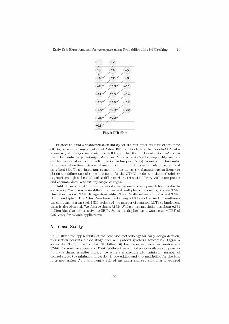
Early Soft Error Analysis for Aerospace using Probabilistic Model Checking 11

+1 +2

*3 +5*4

+6 +8*7

+9 +11*10

+12 +14*13

+15 +17*16

+18 +20*19

+21

+23

*22

Fig. 5: FIR filter

In order to build a characterization library for the first-order estimate of soft erroreffects, we use the bitgen feature of Xilinx ISE tool to identify the essential bits, alsoknown as potentially critical bits. It is well known that the number of critical bits is lessthan the number of potentially critical bits. More accurate SEU susceptibility analysiscan be performed using the fault injection techniques [22, 18], however, for first-orderworst-case estimation, it is a valid assumption that all the essential bits are consideredas critical bits. This is important to mention that we use the characterization library toobtain the failure rate of the components for the CTMC model and the methodologyis generic enough to be used with a different characterization library with more preciseand accurate data, without any major changes.

Table 1 presents the first-order worst-case estimate of component failures due tosoft errors. We characterize different adder and multiplier components, namely 32-bitBrent-kung adder, 32-bit Kogge-stone adder, 32-bit Wallace-tree multiplier and 32-bitBooth multiplier. The Xilinx Synthesis Technology (XST) tool is used to synthesizethe components from their HDL codes and the number of required LUTs to implementthem is also obtained. We observe that a 32-bit Wallace-tree multiplier has about 0.134million bits that are sensitive to SEUs. So this multiplier has a worst-case MTBF of9.22 years for avionic applications.

5 Case Study

To illustrate the applicability of the proposed methodology for early design decision,this section presents a case study from a high-level synthesis benchmark. Figure 5shows the CDFG for a 16-point FIR Filter [16]. For the experiments, we consider the32-bit Kogge-stone adders and 32-bit Wallace tree multipliers as available componentsfrom the characterization library. To achieve a schedule with minimum number ofcontrol steps, the minimum allocation is two adders and two multipliers for the FIRfilter application. At a minimum a pair of one adder and one multiplier is required

93

12 K. A. Hoque, O. A. Mohamed, Y. Savaria and C. Thibeault

for successful operation. The first part of the case study presents the dependabilityanalysis on different configurations. The later part of the case study focuses on theperformance-area trade-off analysis using overall reward calculation.

Table 2: Model construction statistics

Configuration No. of states No. of transitions Time (s)

2A 2M 9 24 0.0022A 3M 12 34 0.0023A 2M 12 34 0.0023A 3M 16 48 0.002

Table 2 shows the statistics and model construction time in PRISM for four differ-ent configurations. The first configuration consists of two adders and two multiplierswith no redundancy. The second and third configuration consists of one spare multiplierand one spare adder respectively used as redundant components (coldspare). Config-uration 4 is equipped with full component-level redundancy, with a spare of each typeof components. All the four configurations have approximately the same model gener-ation time around 0.002 seconds. Configuration 4 has maximum number of states andand maximum number of transitions in the generated Markov model.

Table 3: Configurations vs classes of states

Configurations Operational Degraded Failed(days) (days) (days)

2A 2M 3212.16 419.81 18.022A 3M 3212.16 434.64 3.203A 2M 3212.16 421.45 16.393A 3M 3212.16 436.28 1.55

Probabilistic model checking allows us to reason about the probability of occurrenceof an event or of reaching a state within a specific time period, or at any point oftime in the lifetime of the system. Such measures can be formalized using CSL as P

= ? ( F[t1, t2] "operational"), which must be read as follows: “the probability thatthe system is operational within the specified time-bound where [t1, t2] ∈ R”. In table3, we analyze the number of days the design spends in different classes of states fora mission time of 10 years with a scrub rate of 6 months. The first column of thetable shows the different configurations for evaluation. The second, third and fourthcolumn presents the number of days the design spends in different classes of states.All the configurations spend approximately similar number of days in operational state(rounded to 2 decimal points). Configuration 1 spends around 18 days in failed state.Interestingly, we observe that adding an extra adder as spare does not help muchwhereas adding an extra multiplier as spare significantly reduces the number daysspent in failed state. In configuration 4, the added spares for both adder and multiplierprovide the best result in terms of dependability. This is obvious but will cost morearea on the FPGA. Configuration 1 spends the least number of days in degraded stateand configuration 4 spends the highest number of days in degraded state. For manysafety-critical applications, low performance for a period of time is acceptable. Forsuch systems the number of days spent in failed state is a major concern and hence,configuration 4 and configuration 2 are the two best candidates.

94

Early Soft Error Analysis for Aerospace using Probabilistic Model Checking 13

Fig. 6: Failure Probability vs Scrub rate (days)

Table 4: Scrub rate vs Classes of states

Scrub rate Operational Degraded Failed(months) (days) (days) (days)

1 3567.06 82.87 0.064 3343.21 305.49 1.307 3151.41 494.09 4.4910 2985.99 654.35 9.65

Choice of scrub rate affects the dependability of the system. Table 4 shows theeffects of different scrub rates on configuration 2 for a mission time of 10 years. Fromthe experimental results, we observe that the increase in the scrub rate increases thenumber of days spent in failed and degraded states. Thus, it decreases the numberof days spent in operational state. For a scrub rate of 10 months, the system spendsaround 10 days in failed state whereas for a scrub rate of 4 months, the design spendsonly around 1 days in failed state. For a scrub rate of 1 month, the system spendonly around 1.5 hours in failed state. Such an analysis can help designers to choose aneffective scrub rate best suited for the application.

In figure 6 and table 5, we compare the four available configurations with respectto different scrub rates to calculate their failure probability for the same mission time.The experimental results show that for configuration 1, the failure probability variesfrom 0.020 to 0.145. Configuration 2 has a lower failure probability than configuration3 for all the scrub rates. The failure probability of configuration 4 for all different scrubrates shows the best result with associated extra area overhead.

Table 5: Scrub rate vs configurations

Scrub rate (Months) 2A 2M 2A 3M 3A 2M 3A 3M

1 0.020 0.002 0.019 3.36E-44 0.071 0.011 0.066 0.0047 0.111 0.022 0.104 0.01110 0.145 0.035 0.135 0.020

Steady state analysis of a design is useful to evaluate its dependability in the long-run. The steady-state properties can be formalized using CSL as S = ? [fail], whichmust be read as follows: “the long-run non-availability of the system”, i.e. the steady-

95

14 K. A. Hoque, O. A. Mohamed, Y. Savaria and C. Thibeault

state probability that the system is in failed state. The results of steady-state analysisis presented in table 6 for a scrub rate of 4 months. From the results, we observe thatconfiguration 2 is really an attractive alternative to configuration 4. On the other hand,configuration 1 and configuration 3 offer similar results (rounded to 2 decimal points)over the long-run.

Table 6: Steady state analysis

Class 2A 2M 2A 3M 3A 2M 3A 3M

Fail 0.002 3.86E-4 0.002 1.58E-4Degraded 0.084 0.086 0.084 0.086

Operational 0.913 0.913 0.913 0.913

For throughput-area trade-off analysis, Table 7 shows the long-run overall rewardcalculation for the configurations with a scrub rate of 4 months. The rewards are setupso that the area and expected throughput have equal weights. For every configuration,the maximum throughput is used to normalize the throughput for other states in theMarkov reward model. Similarly, the maximum area is used to normalize the other areavalues among different configurations. The normalized long-run expected throughputfor each configuration is shown in column 2. Column 3 shows the area of each config-uration and their normalized value is shown in column 4. Column 5 shows the overallarea-throughput reward for each configuration. The reward for each configuration iscalculated by multiplying the value of column 2 with the reciprocal of the normalizedarea. Based on the equal reward weighting, configuration 1, which has no redundancy(spare components), shows the best throughput-area reward. This indicates that theextra reliability provided by the redundancy is not always useful to suppress the ex-tra area overhead. However, rescheduling with scrubbing is good enough to serve as afault recovery and repair mechanism in such cases. Another important observation isthat adding a spare multiplier significantly improves the throughput-area reward, muchmore than adding a spare adder. It clearly show, how the inclusion of throughput-areametrics can influence design decisions toward solutions that differs from those result-ing from an analysis based on a dependability metric alone, as in Table 3. Such ananalysis, using the proposed methodology, can be very useful at early design stages fordesigners of safety-critical applications concerned with dependability, performance andarea constraints.

Table 7: Overall reward calculation

Configurations Expected Area Normalized OverallThroughput Area Reward

2A 2M 0.983 1710 0.667 1.462A 3M 0.991 2432 0.948 1.043A 2M 0.990 1834 0.715 1.393A 3M 0.999 2565 1.000 0.99

6 Conclusion

This paper illustrated how probabilistic model checking, a formal verification techniquewhich has already been applied to a wide range of domains, can be used to analyze

96

Early Soft Error Analysis for Aerospace using Probabilistic Model Checking 15

designs at early stage for avionic applications. The design options are modeled using aMarkov reward model, that captures the possible failures, recoveries and repairs possi-ble in high-altitude radiation environment. Afterwards, a wide range of properties areverified to evaluate the design options, in terms of throughput, area and dependability.Such analysis is useful to reduce the overall design cost and effort. A FIR filter casestudy demonstrated how the proposed methodology can be applied to drive the designprocess. Future works include automation of the process to generate the PRISM codefor a given configuration and to analyze designs in the presence of other kinds of faultssuch as Single-Event Functional Interrupts (SEFI).

7 Acknowledgments

This research work is a part of the AVIO-403 project financially supported by theConsortium for Research and Innovation in Aerospace in Quebec (CRIAQ), Fonds deRecherche du Quebec - Nature et Technologies (FRQNT) and the Natural Sciencesand Engineering Research Council of Canada (NSERC). The authors would also liketo thank Bombardier Aerospace, MDA Space Missions and the Canadian Space Agency(CSA) for their technical guidance and financial support.

References

1. P. Adell, G. Allen, G. Swift, and S. McClure. Assessing and mitigating radiationeffects in Xilinx SRAM FPGAs. In Radiation and Its Effects on Components andSystems (RADECS), 2008 European Conference on, pages 418–424, 2008.

2. C. Baier, J-P. Katoen, and H. Hermanns. Approximate symbolic model checkingof continuous-time markov chains (extended abstract), 1999.

3. M. D. Beaudry. Performance-related reliability measures for computing systems.Computers, IEEE Transactions on, C-27(6):540–547, 1978.

4. B. R. Borgerson and R. F. Freitas. A reliability model for gracefully degradingand standby-sparing systems. IEEE Trans. Comput., 24(5):517–525, May 1975.

5. A. Salazar C. Carmichael, M. Caffrey. Correcting Single-Event Upsets throughVirtex Partial Configuration (XAPP216 v1.0), Xilinx corporation, 2010.

6. C. Carmichael. Triple module redundancy design techniques for virtex FPGAs(XAPP197 v1.0.1), Xilinx corporation, 2006.

7. K. Chapman. Virtex-5 SEU critical bit information: Extending the cabability ofthe virtex-5 SEU controller, Xilinx corporation, 2010.

8. E. M. Clarke, E. A. Emerson, and A. P. Sistla. Automatic verification of finite-state concurrent systems using temporal logic specifications. ACM Transactionson Programming Languages and Systems, 8:244–263, 1986.

9. P. Coussy, C. Chavet, P. Bomel, D. Heller, E. Senn, and E. Martin. GAUT: A high-level synthesis tool for dsp applications. In P. Coussy and A. Morawiec, editors,High-Level Synthesis, pages 147–169. Springer Netherlands, 2008.

10. G. Aigner et al. The SUIF program representation. http://suif.stanford.edu/

suif/suif2/index.html, January 2010.

11. J. Heiner, B. Sellers, M. Wirthlin, and J. Kalb. FPGA partial reconfigurationvia configuration scrubbing. In Field Programmable Logic and Applications, 2009.FPL 2009. International Conference on, pages 99–104, 2009.

97

16 K. A. Hoque, O. A. Mohamed, Y. Savaria and C. Thibeault

12. I. Hong, M. Potkonjak, and R Karri. Heterogeneous BISR-approach using systemlevel synthesis flexibility. In Design Automation Conference 1998. Proceedings ofthe ASP-DAC ’98. Asia and South Pacific, pages 289–294, 1998.

13. C. Hu and S. Zain. NSEU mitigation in avionics applications (XAPP1073 (v1.0)may 17, 2010), October 2011.

14. R. Huslende. A combined evaluation of performance and reliability for degradablesystems. In Proceedings of the 1981 ACM SIGMETRICS conference on Measure-ment and modeling of computer systems, pages 157–164. ACM, 1981.

15. ISOGraph. http://www.isograph-software.com.16. R Karri and A. Orailoglu. High-level synthesis of fault-secure microarchitectures.

In Design Automation, 1993. 30th Conference on, pages 429–433, 1993.17. K.M. Kavi, B.P. Buckles, and U. Narayan Bhat. A formal definition of data flow

graph models. Computers, IEEE Transactions on, C-35(11):940–948, 1986.18. P. Kenterlis, N. Kranitis, A. M. Paschalis, D. Gizopoulos, and M. Psarakis. A

low-cost SEU fault emulation platform for SRAM-based FPGAs. In IOLTS, pages235–241, 2006.

19. V. V. Kumar, R. Verma, J. Lach, and J. Bechta Dugan. A markov reward model forreliable synchronous dataflow system design. In Dependable Systems and Networks,2004 International Conference on, pages 817–825, 2004.

20. V.V. Kumar and J. Lach. IC modeling for yield-aware design with variable defectrates. In Reliability and Maintainability Symposium, 2005. Proceedings. Annual,pages 489–495, 2005.

21. A. Lesea. Continuing experiments of atmospheric neutron effects on deep submi-cron integrated circuits (WP286 v1.1), October 2011.

22. W. Mansour and R. Velazco. SEU fault-injection in VHDL-based processors: Acase study. J. Electronic Testing, 29(1):87–94, 2013.

23. P. G. Paulin and J. P. Knight. Force-directed scheduling for the behavioral syn-thesis of asics. Computer-Aided Design of Integrated Circuits and Systems, IEEETransactions on, 8(6):661–679, 1989.

24. PRISM. http://www.prismmodelchecker.org.25. A.M. Saleh, J.J. Serrano, and J.H. Patel. Reliability of scrubbing recovery-

techniques for memory systems. Reliability, IEEE Transactions on, 39(1):114–122,1990.

26. R. M. Smith, K.S. Trivedi, and A.V. Ramesh. Performability analysis: measures,an algorithm, and a case study. Computers, IEEE Transactions on, 37(4):406–417,1988.

27. W. J. Stewart. Introduction to the numerical solution of Markov Chains. PrincetonUniversity Press, 1994.

28. C. Thibeault, Y. Hariri, S. R. Hasan, C. Hobeika, Y. Savaria, Y. Audet, and F. Z.Tazi. A library-based early soft error sensitivity analysis technique for SRAM-based FPGA design. J. Electronic Testing, 29(4):457–471, 2013.

29. S. Tosun, N. Mansouri, E. Arvas, and Yuan Xie. Reliability-Centric High-LevelSynthesis. In Proc. of DATE, 2005.

30. Device reliability report: Second quarter (UG116 v9.1), Xilinx corporation, 2012.

98

TTM/PAT: Specifying and VerifyingTimed Transition Models

Jonathan S. Ostroff1, Chen-Wei Wang1, Yang Liu2, Jun Sun3 and SimonHudon1

1 Department of Electrical Engineering and Computer Science, York University2 School of Computer Engineering, Nanyang Technological University

3 Singapore University of Technology and Design

Abstract. Timed Transition Models (TTMs) are event-based descrip-tions for specifying real-time systems in a discrete setting. We proposea convenient and expressive event-based textual syntax for TTMs anda corresponding operational semantics using labelled transition systems.A system is specified as a composition of module instances. Each modulehas a clean interface for declaring input, output, and shared variables.Events in a module can be specified, individually, as spontaneous, fair orreal-time. An event action specifies a before-after predicate by a set of(possibly non-deterministic) assignments and nested conditionals. TheTTM assertion language, linear-time temporal logic (LTL), allows ref-erences to event occurrences, including clock ticks (thus allowing for acheck that the behaviour is non-Zeno). We implemented a model checkerfor the TTM notation (using the PAT framework) that includes an editorwith static type checking, a graphical simulator, and a LTL verifier. Thetool automatically derives the tick transition and implicit event clocks,removing the burden of manual encoding them. The TTM tool performssignificantly better on a nuclear shutdown system than the manuallyencoded versions analyzed in [6].

Keywords: real-time systems, specification, verification, timed transi-tion models, fairness, model checking

1 Introduction

Checking the correctness of real-time systems is both challenging and importantfor industrial applications. In [6], the authors find it convenient to use a TimedTransition Model (TTM) to describe and verify a nuclear reactor shutdown sys-tem. A graphical statechart-based model checker for TTMs developed in [7] isno longer supported.

To verify the correctness of the shutdown system, authors of [6] manuallytranslate TTMs into timed automata and discrete transition systems, and per-form the real-time verification using, respectively, the Uppaal [5] and SAL [3]model checkers. Real-time models of substantial systems tend to be complex.The manual translation of a TTM to other formats (as in [6]) is time consumingand error prone, may introduce extra states or transitions in the process, andmakes it hard to trace the generated counterexamples back to the original model.

99

2 Jonathan S. Ostroff, Chen-Wei Wang, Yang Liu, Jun Sun and Simon Hudon

In this paper, we develop a new and convenient event-based notation forTTMs consisting of a textual syntax and formal operational semantics. Theone-step semantics allows us to use the PAT toolset [10, 9] to develop an explicitstate model checker for the new notation. The resulting model checker performssignificantly better than the manually encoded model using other tools, at thesame time bypassing the need to do manual translation. The new model checkerhas good support for type checking, visual simulation, and convenient counter-example traceability back to the model.

The event-based syntax also makes the language amenable to formal rea-soning using theorem proving in the spirit of Event-B [1] and compositionalreasoning. This provides a timed extension to the Event-B notation (although,in this paper, we do not consider refinement).

Outline and Contributions. This paper presents three main contributions. First,our new TTM notation allows for the description of a variety of discrete reactivesystems (see Section 2 for a pacemaker example) by cooperating modules thatcontain variables and events. Events have implicit clocks for imposing lower andupper time bounds on their occurrences. Our notation also supports sponta-neous, fair, and timed behaviours at both the event level and the system level.Timers are explicit clocks that may be used to constrain system behaviour.Second, we develop a formal operational semantics with digitization (see Sec-tion 3) that is amenable to automated tool support. Third, we implement theTTM/PAT tool for specifying and verifying TTMs (see Section 4 for its eval-uation). System properties can be expressed in the linear-time temporal logic(LTL) and may refer to timers and event occurrences (see Section 3 for repre-senting event occurrences as state predicates). The properties language directlysupports healthiness checks such as non-Zeno behaviour1 and the monotonicityof timers. More details on the tool and experimental data are discussed in anextended report [8], and the grammar of TTM textual syntax and the tool areavailable at https://wiki.eecs.yorku.ca/project/ttm/.

2 A Small Pacemaker Example

We use a small pacemaker example (similar to the one in [4]) to illustrate thereal-time features of TTMs. A cardiac pacemaker is an electronic device im-planted into the body to regulate the heart beat by delivering electrical stimuli(called paces) over leads with electrodes that are in contact with the heart. Thepacemaker may also detect (or sense) natural cardiac stimulations.

A pacemaker in the VVI mode operates in a timing cycle that begins witha ventricular pacing or sensing. The basis of the timing cycle is the lower rateinterval (LRI=1000ms): the maximum amount of time between two consecutiveventricular sensing. If the LRI elapses and no sensing has occurred since thebeginning of the cycle, a pace is delivered and the cycle is reset. On the otherhand, if a heart beat is sensed, the cycle is reset without delivering a pace.

1 In TTM/PAT we consider a discrete time domain, where there is an explicit transi-tion for the tick of a global clock. Zeno behaviour then denotes executions in whichthe tick transition does not occur infinitely often (i.e., at some point, time stops).

100

TTM/PAT: Specifying and Verifying Timed Transition Models 3

At the beginning of each cycle, there is a ventricular refractory period (VRP= 400ms): chaotic electrical activity that immediately follows a heart beat, andmay lead to spurious sensing that interferes with future pacing. Sensing is there-fore disabled during the VRP period. Once the VRP period is over, a ventricularsensing inhibits the pacing and resets the LRI, starting a new timing cycle.

In the VVI mode, hysteresis pacing can be enabled to delay pacing beyondthe LRI in order to give the heart a chance to resume the normal operation. Inthat case, the timing cycle is set to a larger value, namely the hysteresis rateinterval (HRI=1200ms). It becomes enabled after a natural heart beat has beensensed. In [4], hysteresis pacing is enabled after a ventricular sense is received,and disabled after a pacing signal is sent.

Using the textual syntax of TTM, we define constants and a timer t for thecardiac cycle as follows:

#define VRP 400;#define LRI 1000;#define HRI 1200;

timerst: 0..(HRI+1)

enabledinitend

share initializationsense: BOOL = falsepace: BOOL = false

end

Timer t has a range from zero to HRI+1, and it is initially zero and enabled.When the value of t reaches one beyond HRI + 1, it stops counting up and itsmonotonicity predicate, mono(t), becomes false. This predicate holds so long asthat timer t is ticking in synch with a tick of a global clock, and that it is notstopped or restarted (see Section 3). The tick transition is an implicit transi-tion (i.e., it is not given by the text of a TTM) representing the ticking of aglobal clock. The tick transition increments timers and implicit clocks associ-ated with events. We also defined shared variables sense and pace to represent,respectively, a ventricular sensing or pacing.

We declare a module template for the heart as follows:

module HEARTinterface

pace: share BOOLsense: share BOOL

localri : INT = HRIlast ri: INT = HRIpc: INT = 0

eventshbn[VRP, ∗] // natural heart beatwhen !pace && pc==0do sense := true,

ri := HRI,last ri:=ri,pc := 1

end

hbp[0,0] // paced heart beatwhen pace && VRP <= t && pc==0do pace := false,

ri := LRI ,last ri := ri,pc := 1

end

new cycle[0,0] // restart a new cyclewhen pc==1start tdo pc := 0end

101

4 Jonathan S. Ostroff, Chen-Wei Wang, Yang Liu, Jun Sun and Simon Hudon

The interface of module template HEART declares the access to shared variablessense and pace. The local variable ri (rate interval) is either HRI or LRI de-pending on whether hysteresis pacing is enabled. Likewise last ri records the lastvalue of the rate interval. They are auxiliary variables: they annotate the sys-tem state without affecting2 the behaviours and are used in LTL specifications.Variable pc (program counter) is used as a sequencing mechanism for events.

The heart module has a natural heartbeat (event hbn) and a paced heartbeat(event hbp). If there is a natural heart beat, then the sense flag is set, ri is set toHRI, and the last rate interval is also recorded in last ri. After the VRP period,it is also possible for a paced heart beat to occur if the pace flag is set. Thuspace ∧VRP ≤ t is part of the guard of the urgent event hbp[0, 0]. After either anatural or paced heart beat, the timer t is restarted by the new cycle event andthe cardiac cycle begins again.

A natural heart beat might occur at any time after the ventricle refractorydelay VRP, or it might never occur. Thus the lower time bound of hbn is VRPand the upper time bound is ∗ (i.e ∞). If the upper time bound is ∗ then wehave a spontaneous event (i.e., an event that is not urgent or forced to occur).We can thus accommodate a variety of fairness assumptions (discussed furtherin Section 3), including spontaneous events, just or compassionate events, andreal-time events that must occur between their lower and upper time bounds.An urgent event e[0, 0] is one that must occur before the next tick of the globalclock (provided its guard continuously remains true).

We formulate the requirements using linear time temporal logic (LTL) solelyin terms of the phenomena of the environment (i.e., the heart) as follows:

R1: �♦((H.hbn∨H.hbp) ∧ (V RP ≤ t ≤ HRI)).3 Infinitely often, a natural orpaced heart beat occurs between VRP and HRI time units from each other.

R2: �(H.hbn → (VRP ≤ t ≤ H.last ri)). A natural heartbeat occurs onlyin the closed interval [VRP, H.last ri] in the cardiac cycle. H.last ri recordsthe required rate interval in the heart for the last complete cycle, either LRIor HRI, depending upon whether hysteresis pacing has been properly enabled.Thus, �((H.last ri=LRI) ∨ (H.last ri=HRI)) also holds.

R3: �(H.hbp → (t = H.last ri)). A paced heart beat occurs only if the timert is at the relevant rate interval. The ventricle controller will have to estimateH.ri (which, as opposed to H.last ri, relates to the current cycle) in order toensure that the heart paces according to this requirement.

There is a concern that some event (either in the heart module or elsewhere)might illegally set the timer t to a value that makes the specification triviallytrue. Of course, in a small system, inspection of the TTMs (or timed automatain the case of Uppaal) might re-assure us that all is well. Nevertheless, it wouldbe advantageous to check that timers tick monotonically and uninterruptedly.Thus each TTM timer t must be equipped with a corresponding monotonicity

2 Variables ri and last ri are used in neither event guards nor the right hand side ofassignments to non-auxiliary variables

3 H.hbn designates the event hbn in module instance H. The same syntax works forlocal variables as well.

102

TTM/PAT: Specifying and Verifying Timed Transition Models 5

predicate mono(t) that holds so long as timer t is not stopped or restarted (seeSection 3). We may thus check (�♦H.new cycle)∧�(H.new cycle→ t = 0) and�(H.new cycle → mono(t)U( (H.hbn ∨H.hbp) ∧ (V RP ≤ t ≤ HRI) )), whichguarantee that there is an appropriate heart beat in each cardiac cycle.

When using events with upper time bound 0, we must provide a way ofchecking Zeno behaviour [7]. We can directly check that time always progresseswith the LTL formula �♦tick. The tick event is implicit. That is, it is automat-ically constructed by the tool with the precise semantics described in Section 3.The ability to refer to the occurrences of events in the TTM assertions makesit possible to specify the required behaviour more directly than in other tools,e.g. Uppaal. We now devise a ventricle controller whose cooperation with theheart will satisfy requirements R1 to R3.

module VENTRICLE CONTROLLERinterface

pace : share BOOLsense: share BOOL

localri : INT = HRI; pc: INT = 0

eventsvpace[0,0]when pc==0 && !sense && t==rido ri := LRI, pace := true, pc:= 1end

vsense[0,0]when pc==0 && sensedo ri := HRI, sense := false, pc :=1end

compute delay[1,1]when pc==1do pc:= 0end

end

The controller maintains its own estimate VC.ri of the heart’s rate interval H.ri,where VC and H are module instances that we construct below. We may nowcompose the heart together with the controller as follows:

instancesH = HEART

(share pace, share sense)VC = VENTRICLE CONTROLLER

(share pace, share sense)endcomposition

System = H || VCend

#define rt (t=H.last ri);#define t0 (t=0);#define wr VRP <= t && t <= HRI;#assert System |= [](H.hbp −> rt);#assert System |= []<>(H.new cycle && t0);#assert System |=

[](H.new cycle && t0 −>mono(t) U ((H.hbn || H.hbp) && wr));

#assert System |= []<>tick;

The above syntax is accepted by the TTM/PAT tool, and all the requirementsare verified in a few seconds. The syntax also allows us to compose an indexed setof instances. For example, in Fischer’s mutual exclusion algorithm (Section 4.2),we write:

composition fischer = || i: 1..n @ PROCESS(share x, share c, in i) end

More details on this example is discussed in an extended report [8].

103

6 Jonathan S. Ostroff, Chen-Wei Wang, Yang Liu, Jun Sun and Simon Hudon

3 TTM Syntax and Semantics

Section 2 provides an example of the new concrete textual syntax for TTMs. Inthis section, we provide a one-step operational semantics for TTMs.

3.1 Abstract Syntax. Following [7] and using the mathematical conven-tions of Event-B [1], we define the abstract syntax of a TTM module instanceMas a 5-tuple, i.e.,M = (V, s0, T, t0, E) where 1) V is a set of variable identifiers,declared local or in a module interface; 2) T is a set of timer identifiers; 3) E isa set of events that may change the state; 4) s0 ∈ STATE is the initial variableassignment, with STATE , V → VALUE; and 5) t0 ∈ TIME is the initialtimer assignment, with TIME , T → N.

Concrete syntax of event e:

event id [l,u] justwhen grdstart t1, t2stop t3, t4do v1 := exp1,

if condition then v2 := exp2else skip fi,v3 :: 1..4

end

Abstract syntax of the event e:

– e.id ∈ ID;– e.l ∈ N;– e.u ∈ N ∪ {∞}– e.fair ∈ {spontaneous, just, compassionate}– e.grd ∈ STATE× TIME→ BOOL;– e.start ⊆ T ;– e.stop ⊆ T ;– e.action ∈ STATE× TIME↔ STATE;

Fig. 1: Concrete and Abstract syntax of TTM events

We use an 8-tuple (id, l, u, fair, grd, start, stop, action) to define the abstractsyntax of an event e, and we use the dot notation “.” to access the fields, as shownon the right of Fig. 1. The string identifier of an event e is written as e.id. Theguard of event e, i.e., e.grd, is any Boolean expression in V and T . For example,on the left of Fig. 1, we have V = {v1, v2, v3, · · · } and T = {t1, t2, t3, t4, · · · }.Functions boundt ∈ T→N and type ∈ T→P(N) provide, respectively, the upperbound and the type of each timer. For example, if timer t1 is declared in theTTM as t1 : 0..5, then boundt(t1) = 5 and type(t1) = {0..6}. As will be detailedbelow, timers count up to one beyond the specified bound at which point theyremain fixed until they are restarted.

An event e must be taken between its lower time bound e.l and upper timebound e.u, provided that its guard e.grd remains true. The event action involvessimultaneous assignments to v1, v2, · · · . The notation v3 :: 1..4 is an example of ademonic assignment in which v3 takes any value from 1 to 4. All the assignmentsin the event action are applied simultaneously in one step.

In an assignment y := exp, the expression on the right may use primed (e.g.x′) and unprimed (e.g. x) state variables as well as the initial value of timers. Avariable with a prime refers to the variable’s value in the next state and a variablewithout prime refers to its value in the current state. The use of primed vari-ables in expressions allows for simpler and more expressive descriptions of state

104

TTM/PAT: Specifying and Verifying Timed Transition Models 7

changes. The state changes effected by an event e is described in the abstractsyntax by a before-after predicate e.action. The concrete syntax also allows forassignments to be embedded in (possibly nested) conditional statements.4

3.2 Formal Semantics. We provide a one-step operational semantics ofa TTM module instance M in LTS (Labelled Transition Systems).

Definition: LTS: Given a TTM module instance M, an LTS (Labelled Tran-sition System) is a 4-tuple L = (Π,π0,T,→) where 1) Π is a set of systemconfigurations; 2) π0 ∈ Π is an initial configuration; 3) T is a set of transitionsnames; and 4) → ⊆ Π ×T×Π is a transition relation.

We now describe the LTS semantics of TTMs. Let Eid , {e ∈ E • e.id}be the set of event names (identifiers). A configuration π ∈ Π is defined by a6-tuple (s, t,m, c, x, p). We explain each of the six components as follows:

• s ∈ STATE is a value assignment for all the variables of the system. The statecan be read and changed by any transition corresponding to an event in E.

• t ∈ TIME is a value assignment for the timers of the system. Events (andhence their corresponding transitions) may only start, stop and read timers. Aswill be discussed below, we introduce a special transition, called tick, which alsochanges the timers. Timers ti that are stopped have values boundt(ti) + 1.

•m ∈ T→BOOL records the status of monotonicity of each timer. Suppose evente1 in a TTM starts t1. In LTL we might write �( e1 ∧ t1 = 0 → ♦(q ∧ t1 ≤ 4) )(note that t1 = 0 is redundant) to specify that q becomes true within 4 timeunits of event e1 occurring. However, other events might stop or restart t1 beforeq is satisfied hence breaking the synchronicity between t1 and a global clock.5

Instead, we express the intended property as �( e1∧t1 = 0 → m(t1) U (q∧t1 ≤4) ). The expression m(t1) (standing for monotonicity of t1) holds in any statewhere t1 is not stopped or being reset. We explain monotonicity further below.

• c ∈ Eid → N ∪ {−1} is a value assignment for a clock implicitly associatedwith each event. These clocks are used to decide whether an event has beenenabled for long enough and whether it is urgent. An event e ∈ E is enabledwhen its clock’s value is between the event’s lower time bound (i.e., e.l) andits upper time bound (i.e., e.u). Furthermore, the type (or range) of c(e.id) is{−1, 0, ...e.u}. When an event’s clock is disabled, as opposed to the conventionused with timers, the clock’s value is −1.

4 With all the complexity of structures allowed by the syntax of actions, sequentialcomposition is not allowed. This is in an effort to make actions into specificationsrather than implementations. This would allow us to generalize TTMs to allow anEvent-B style of symbolic reasoning.

5 Suppose that event e2 also starts t1, that e3 establishes q and that the events occur

in the following order: π0e1→ π1

t1=0

tick3

→ π4t1=3

e2→ π5t1=0

tick2

→ π7t1=2

e3→ π8t1=2 ∧ q

· · · . This

execution satisfies the first LTL formula but does not satisfy the intended specifica-tion: when q becomes true, t1 = 2 but it is 5 ticks away from the last occurrence ofe1.

105

8 Jonathan S. Ostroff, Chen-Wei Wang, Yang Liu, Jun Sun and Simon Hudon

• x ∈ Eid ∪ {⊥} is used as a sequencing mechanism to ensure that each tran-sition e is immediately preceded by an e# transition whose only function isto update the monotonicity record m. For example, in the following execution

· · · e1→ π1x=⊥

e2#→ π2x=e2

e2→ π3x=⊥→ · · · , suppose in π1 the value of timer t2 is 3 and

that e2 restarts t2. Then, in π2, we have x = e2 ∧ t2 = 3 ∧ m(t2) = false. Inπ3, we have x = ⊥ ∧ t2 = 0 ∧ m(t2) = true. In order to record the breakingof monotonicity, the e2# transition sets m(t2) to false, which gets set back totrue in the next execution step. The precise effect of these transitions will bedescribed below.

• p ∈ Eid ∪ {tick,⊥} holds the name of the last event to be taken at eachconfiguration. It is ⊥ in the initial configuration as no event has yet occurred. Itallows us to refer to events in LTL formulas in order to state that they have justoccurred. For instance, in the formula above, (s, t,m, p) |= e1 ∧ t1 = 0 (whichreads: the configuration satisfies the formula) evaluates to p = e1 ∧ t(t1) = 0.

Given a flattened module instance M, the transitions of its correspondingLTS are given as T = Eid ∪ E# ∪ {tick}. As explained above, for each evente ∈ E, we introduce a monotonicity breaking transition e.id#. We thus defineE# , {e ∈ E • e.id#}. The tick transition represents one tick of a globalclock. Explicit timers and event lower and upper time bounds are described withrespect to this tick transition. We define the enabling condition of event e ∈ E ase.en , e.grd ∧ e.l ≤ e.c ≤ e.u, where e.c evaluates to c(e.id) in a configurationwhose clock component is c. Thus an event is enabled in a configuration thatsatisfies its guard and where the event’s implicit clock is between its lower andupper time bound.

The initial configuration is defined as π0 = (s0, t0,m0, c0,⊥,⊥), where s0and t0 come from the abstract syntax of the TTM. m0 and c0 are given by:

m0(ti) ≡ t0(ti) = 0

c0(ei.id) =

{0 (s0, t0) |= ei.grd

−1 (s0, t0) 6|= ei.grd

for each ti ∈ T and ei ∈ E. It is implicit in the above formula that m0(ti)depends only on whether or not ti is initially enabled (specified using the keywordenabledinit or disabledinit). If the keyword enabledinit is specified, t0(ti) =0; otherwise, if the keyword disabledinit is specified, t0(ti) = boundt(ti) + 1.

An execution σ of the LTS is an infinite sequence, alternating between con-figurations and transitions, written as π0

τ1→ π1τ2→ π2 → · · · where τi ∈ T and

πi ∈ Π. Below, we provide constraints on each one-step relation (πe→ π′) in

an execution. If an execution σ satisfies all these constraints then we call σ alegal execution. We let ΣL denote the set of all legal executions of the labelledtransition system L. The set ΣL provides a precise and complete definition ofthe behaviour of L. If a state-formula q holds in a configuration π, then we writeπ � q. In some formulas, such as guards, all the components of a configurationare not necessary. We express this by dropping some components of the config-uration on the left of the double turnstile (|=), as in (s0, t0) |= e.grd. Given a

106

TTM/PAT: Specifying and Verifying Timed Transition Models 9

temporal logic property ϕ and an LTS L, we write L � ϕ iff ∀σ ∈ ΣL • σ � ϕ.The three possible transition steps are:

(s, t,m, c,⊥, p) e#→ (s, t,m′, c, e, p) (3.1)

(s, t,m, c, e, p)e→ (s′, t′,m′, c′,⊥, e) (3.2)

(s, t,m, c,⊥, p) tick→ (s, t′,m′, c′,⊥, tick) (3.3)Each of the above transitions has side conditions which we now enumerate.

3.2.1 Taking e#. The monotonicity breaking transition e#, specified in Equa-tion 3.1 (p9), is taken only if (s, t, c) � e.en and the x-component of the config-uration is ⊥. For each t ∈ T , m′(t) ≡ t /∈ e.start ∧m(t). This ensures that, fortimer t, just before it is (re)started, m(t) = false. It is set back to true by theimmediately following event, e, and it remains true as long as t is not restartedand has not reached its upper bound. Transition e# modifies only m and x inthe configuration, and thus maintains the truth of (s, t, c) � e.en.

3.2.2 Taking e. The transition e, specified in Equation 3.2 (p9), is taken only if(s, t, c) � e.en and the x-component of the configuration is e. The component s′

of the next configuration in an execution is determined nondeterministically bye.action, which is a relation rather than a function. This means that any nextconfiguration that satisfies the relation can be part of a valid execution, i.e., s′ isonly constrained by (s, t, s′) ∈ e.action. The other components are constraineddeterministically. The following function tables specify the updates to m, t andc upon occurrence of transition e.

For each timer ti ∈ T m′(ti) t′(ti)

ti ∈ e.start ti ∈ e.stop impossibleti /∈ e.stop true 0

ti /∈ e.start ti ∈ e.stop false boundt(ti) + 1ti /∈ e.stop m(ti) t(ti)

For each event ei ∈ E c′(ei.id)

(s′, t′) 6|= ei.grd -1

(s′, t′) |= ei.grd(s, t) |= ei.grd ∧ ¬ei = e c(ei.id)(s, t) 6|= ei.grd ∨ ei = e 0

In the above, we start and stop the implicit clock of ei as a consequence ofexecuting e, according to whether ei.grd becomes true, is false (i.e., becomes orremains false) or remains true. Since event ei becomes enabled ei.l units afterits guard becomes true, this allows us to know when to consider ei as enabled,i.e., ready to be taken. As a special case, the implicit clock of event e (underconsideration) is restarted when e.grd remains true.

3.2.3 Taking tick. The tick transition, specified in Equation 3.3 (p9), is takenonly if ∀e ∈ E • c(e.id) < e.u and the x-component of the configuration is ⊥(thus preventing tick from intervening between any e# and e pair). For anytimer ti ∈ T , the updates to t′, m′ and c′ are:

107

10 Jonathan S. Ostroff, Chen-Wei Wang, Yang Liu, Jun Sun and Simon Hudon

t′(ti) = (t(ti) ↓ boundt(ti)) + 1

m′(ti) ≡ ¬ (t(ti) = boundt(ti)+1)

For each event e ∈ E c′(e.id)

(s′, t′) 6|= e.grd -1

(s′, t′) |= e.grd(s, t) 6|= e.grd 0(s, t) |= e.grd c(e.id) + 1

Thus, tick increments timers and implicit clocks to their upper bounds. Transi-tion tick also marks timers as non-monotonic when they reach their upper boundand reset clocks when the corresponding events are disabled.

3.2.4 Scheduling. So far, we have made no mention of scheduling: we con-strained executions so that the state changes in controlled ways, but a givenexecution may still make no progress. To make progress, we need to assumefairness. In the current implementation of TTM/PAT, the possible schedulingassumptions6 on TTM events are restricted to the following four:

1. Spontaneous event. Even when it is enabled, the event might never be taken.This is assumed when no fairness keyword is given and the upper time bound is* or unspecified.

2. Just event scheduling (also known as weak fairness [10]). For any executionσ ∈ ΣL, if an event e eventually becomes continuously enabled, it has to occurinfinitely many times, that is σ � ♦�e.en → �♦e. This is assumed whenthe keyword just is given next to the event and the upper time bound is * orunspecified. We use e.en and not e.grd in the fairness formula as the event canonly be taken e.l units after its guard became true.

3. Compassionate event scheduling (also known as strong fairness [10]). For anyexecution σ ∈ ΣL, if an event e becomes enabled infinitely many times, it hasto occur infinitely many times, that is σ � �♦e.en → �♦e. This is assumedwhen the keyword compassionate is given next to the event and the uppertime bound is * or unspecified.

4. Real-time event scheduling. The (finite) upper time bound (u) of the event eis taken as a deadline: if the event’s guard is true for u units of time, it has tooccur within u units of after the guard becomes true or after the last occurrenceof e. To achieve this effect, the event e is treated as just. Since tick will not occuras long as e is urgent (i.e., e.c = e.u), transition e will be forced to occur (unlesssome other event occurs and disables it).

To accurately model time, the tick transition is treated as compassionate inthe LTS. This ensures that time progresses except in cases of Zeno-behaviors (dis-cussed below). Spontaneous events cannot be used to establish liveness proper-ties. Justice and compassion are strong enough assumptions to establish livenessproperties but not real-time properties. Finally, real-time events can establishboth liveness and real-time properties.

The above semantics allows for Zeno behaviours which occur when there areloops involving events with zero upper time bound (i.e., e[0, 0]). We could bane[0, 0] events altogether, but that would eliminate behaviours that are feasibleand useful, e.g., where we describe a finite sequence of immediately urgent events

6 The scheduling assumptions are taken care of by the model-checking algorithms [10].

108

TTM/PAT: Specifying and Verifying Timed Transition Models 11

(not in a loop). We can check that the system is non-Zeno by checking that thesystem satisfies �♦tick.

The abstract TTM semantics provided above can be (and has been) im-plemented efficiently. For example, in the abstract semantics every event e ispreceded by a breaker of monotonicity e#. Most of the e# events do not changethe configuration monotonicity component m and can thus be safely omittedfrom the reachability graph thereby shrinking it.

3.3 Semantics of Module Composition. We have specified so far thesemantics of individual TTM machines. However, the TTM notation includes acomposition operator which was not discussed so far. The semantics of systemscomprising many machines is defined through flattening, i.e. by providing a singlemachine which, by definition, has the same semantics as the whole system.

Instantiation. When integrating modules in a system, they first have to be in-stantiated. This means that the interface variables of the module must be linkedto variables of the system it will be a part of. For example if we had a Philmodule with two shared variables, left fork and right fork , and two global forkvariables f1 and f2, we could instantiate them as:

instances p1 = Phil(share f1, share f2) ; p2 = Phil(share f2, share f1) end

This makes f1 the left fork of p1 and the right fork of p1, and makes f2 the leftfork of p2 and the right fork of p1. Philosopher p1 is therefore equivalent to themodule Phil with its references to left fork substituted by f1 and its referencesto right fork substituted by f2.

Composition. The composition m1||m2 is an associative and commutative func-tion of two module instances. Before flattening the composition, we rename thelocal variables and the events so that the name of each local variable will beunique across the whole system. The renaming is done in the variable declara-tions, in the expressions in events, and on the left-hand sides of assignments. Thisis strictly a syntactic change and does not affect the semantics of the instances.

We then proceed to creating the composite machine. Its local variables willbe the (disjoint) union of the local variables of the two instances. Its interfacevariables will be the (possibly non-disjoint) union of the interface variables ofboth instances with their mode (in, out, share) adjusted. The set of the eventsof the composition is the union of the set of events of both machines.

Iterated Composition. Iterated composition is the mechanism that allows us tocompose a number of similar instances without specifying each individually. Forexample, in the case of a network of processes, we may want to specify the pro-cesses once and instantiate them many times with a different process identifier.

system = || pid : PID @ Process(in pid)

where PID is the set of process identifiers. It allows us to change the numberof processes by just changing that set. In this case, if PID = 1..3, the above isequivalent to:

instances p1 = Process(in 1) ; p2 = Process(in 2) ; p3 = Process(in 3) endcomposition system = p1 || p2 || p3 end

109

12 Jonathan S. Ostroff, Chen-Wei Wang, Yang Liu, Jun Sun and Simon Hudon

Nuclear ReactorPressurePower Trip Relay

3s

2s Relay

Pressure

Power

DRT Shutdown Computerboth_hi[1,1] delay[29,29]

power_low[1,1] power_hi[1,1]relay:=open

delay[19,19]

power_hi[1,1]

power_low[1,1]relay:=close

State-Based Model of Controller

Fig. 2: DRT System: Context Diagram and Transition Diagram of Controller

4 Evaluation

In Section 4.1, we report on the performance of our new TTM model checker incomparison with the manual encoding in Uppaal and SAL in [6]. If the systemwas implemented directly in Uppaal (as opposed to using the manual encod-ing from a TTM), the Uppaal results would likely have been much better. Thissection merely shows that if a designer finds the TTM notation more conve-nient to use, then our new tool (1) saves the designer from the effort of manualtranslation, and from resulting error; and (2) performs better than the manuallyencoded version in other formats.

In Section 4.2, we address the current limitation of TTM/PAT, implementedusing digitization, by reporting on its performance on the Fischers mutual ex-clusion algorithm, in comparison with the symbolic model checkers Uppaal andRTS. Experiments were conducted on a 64-bit Windows 7 PC with Intel(R)Core(TM) i7 CPU 860 @ 2.80 GHz (16.0 GB RAM).

4.1 Delayed Reactor Trip System. The DRT (delayed reactor trip)shutdown system, analyzed in [6], is illustrated in Fig. 2. The old implementationof the DRT used timers, comparators and logic gates as shown on the left ofFig. 2. The new DRT system is to be implemented on a microprocessor systemwith a cycle time of 100ms. The system samples the inputs and passes througha block of control code every 0.1 seconds. A high-level state/event description(SPEC ) of the code that replaces the analogue system is shown on the right ofFig. 2 ([6]). When the reactor pressure and power exceed acceptable safety limitsin a specified way, we want the DRT control system to shut down the reactor.Otherwise, we want the control system to be reset to its initial monitoring state.

In [6], the SPEC level TTM description of the controller is refined into alower level PROG description that is closer to implemented code (in a cyclicexecutive). Translations to PVS are used to show that PROG refines SPEC.The reactor itself is represented by a TTM that can change the power and pres-sure levels arbitrarily every .1 seconds (1 tick of the clock), by using a demonicassignment setting them to either low or high. The system thus consists of the

110

TTM/PAT: Specifying and Verifying Timed Transition Models 13

Property Controller ModelTTM: �♦ tick

(s) Result

TTM/PAT

(s)

Uppaal

(s)SAL(s)

Fres:

SystemResponse

SPEC 11 × 11 13 25PROG 31 × 32 24 407SPECr 5 × 3 12 15PROGr 14 × 9 21 330

Fires:

InitializedSystem

Response

SPEC .5 X .4 .9 11PROG 1 X 1 1 20SPECr .3 X .2 .4 7PROGr .8 X .6 1 13

SPECr1||SPECr2 16 X 11 62 235PROGr1||PROGr2 109 X 70 76 >1h

Frec:

SystemRecovery

SPEC .3 × .08 .1 6PROG .8 × .2 .3 7SPECr .1 X .07 .2 4PROGr .3 X .07 .6 5

SPECr1||SPECr2 22 × .06 145 18PROGr1||PROGr2 142 × .1 11 >1h

Table 1: TTM/PAT vs. Uppaal vs. SAL: Delayed Reactor Trip System

controller (either SPEC or PROG) executing in parallel with plant (the reac-tor). The two essential properties that the system must satisfy are:

Response Formula Fres. Henceforth, if Power and Pressure simultaneouslyexceed their threshold values for at least 2 clock ticks, and 30 ticks later Powerexceeds its threshold for another 2 ticks, then within 30 to 32 ticks, open thereactor relay for at least 20 ticks.

Recovery Formula Frec. Henceforth, if the relay is open for 20 ticks, and afterthe 20th tick the power is low for at least 2 ticks, then the relay is closed beforethe 22nd tick.

With the help of an observer and timers, the response formula Fres is rep-resented in LTL by a liveness property �p → ♦q where p and q use timers tocapture the timed response (see [6] for the details). Likewise, the recovery for-mula Frec can be reduced to a safety property �¬(Tw = 2∧relay = open) whereTw is a timer describing a state in which the power has returned to normal for2 ticks of the clock, but the relay is still open.

Both SPEC and PROG did not satisfy Fres due to an error in the observer.Thus, verification of Fres should produce counterexamples in any model checker.Also, it was discovered that there was an error in the controller (in both SPECand PROG) as the recovery property was not satisfied. The revised and correcteddescriptions of the controller are SPECr and PROGr, respectively, whose re-sponse property is referred to as Fires.

To generate large reachability graphs, multiple controllers were run in paral-lel. For example, in checking the response property Fires on PROGr1||PROGr2,the TTM tool explored 421,442 states and 821,121 transitions (in 70 seconds).These systems and their LTL specifications (some valid and some invalid) pro-vide a rich set of examples to test the performance of the various model checkers.

111

14 Jonathan S. Ostroff, Chen-Wei Wang, Yang Liu, Jun Sun and Simon Hudon

Property Result n Uppaal

(s)

PAT/RTSTTM/PAT

(s)clock zone

(s)

digitization

(s)

non-zenoness:�♦ tick X

4

not directly supported

.55 46 317 2308 >1h

P1 mutual exclusion:� (c ≤ 1)

X

4 .04 .12 .08 .265 .1 .2 .4 1.96 .8 2 3 147 14 21 28 1048 563 250 244 7689 >1h 2918 >1h >1h

P2 liveness:�(request→ ♦wait) X

4 .06 .07 .1 .35 .2 .3 .8 36 4 3 6 247 181 29 58 1778 >1h 307 >1h >1h

P3 liveness:�(request→ ♦cs) ×

4 .2 .06 .09 .015 .2 .3 .9 .016 .3 3 19 .037 .2 70 942 .048 .2 2277 >1h .03

Table 2: TTM/PAT vs. RTS/PAT vs. Uppaal: Fischer’s Algorithm

In [6], the TTMs were manually encoded into the Uppaal and SAL model check-ers. The authors of [6] show that, in general, Uppaal performed better than SALgiven its real-time features. The manual encoding of TTMs into Uppaal andSAL is itself a time-consuming process. This is where the new TTM/PAT toolis useful as the encoding is automatic. What about performance? In Table 1,we compare TTM/PAT to the encodings in SAL and Uppaal for response andrecovery, and for the various versions of the controller. The 4th column labelled“Result” has a checkmark where the LTL property is valid; otherwise, the modelchecker produces a counterexample. The 3rd column provides the time it takesto check for non-Zeno behaviour in the TTM tool (not supported in the othertools). In general, TTM/PAT significantly outperforms both encodings in SALand in Uppaal. There is only one exception in the second row for Fres. TTM/-PAT finds the formula invalid in 9 seconds versus 18 seconds for Uppaal (notshown in the table) where a counterexample is not requested. However, it takesTTM/PAT 32 seconds to find the counterexample versus 24 seconds for Uppaal.

4.2 Fischer’s Mutual Exclusion Algorithm. TTM/PAT is an explicitstate tool for discrete systems. The expectation was that it would perform well inthe category of explicit state model checkers. Nevertheless, it was expected thatsymbolic checkers (using timed automata) such as Uppaal would outperform it.In addition, Uppaal is continuous time (although timing constants in Uppaal areintegers) whereas TTMs are discrete time. Nevertheless, the assertion notation of

112

TTM/PAT: Specifying and Verifying Timed Transition Models 15

Assertion TCTL of Uppaal LTL of TTM/PAT

Henceforth p S |= A� p S |= � p

Eventually p S |= A♦ p S |= ♦ pWhenever p, eventually q S |= p −→ q S |= � (p→ (♦ q))Infinitely often p S |= true −→ p S |= �♦ pReferring to a state M.state pc = state

Non-Zenoness × S |= �♦ tickp until q × S |= p U qq releases p × S |= q R p

Nesting of temporal operators × e.g., � (♦ p→ (pUq))Referring to occurrences of event e × e

Timer t has increased monotonically × mono (t)

Eventually henceforth p × S |= ♦� p

S possibly maintains p S |= E� p inverse of S |= ♦ (¬p)S possibly reaches p S |= E♦ p S reaches p

Nesting of path quantifiers × ×∀♦ ∀� p × ×

Table 3: TTM vs. Uppaal: Language of Assertions

TTMs is more expressive than Uppaal (see Section 5 and Table 3) and its event-based syntax is amenable to formal reasoning and compositional reasoning.

A comparison was performed in [9] between RTS (a PAT plugin) and Uppaalusing the Fischer’s mutual exclusion algorithm. We compare the performance ofthe TTM/PAT tool to RTS and Uppaal using the same example. For a propercomparison of the three tools, many more examples would be needed.

Our experiment shows that, in determining that properties P1 (a safetyproperty) and P2 (a liveness property stating that a process requesting accessto its critical section leads it to wait) are valid, the clock zone mode of RTSis faster than Uppaal (see Table 2). The speed of TTM/PAT is within a factorbetween 3 and 4 of the digitization mode of RTS. TTM/PAT is almost as fast asUppaal in producing counterexamples for property P3 (expressing the starvationfreedom property). Results in Table 2 (with n the number of processes put inparallel) suggest that the techniques used in clock zones of RTS and those ofUppaal would provide enhancements for more efficient verification of TTMs.

5 Conclusion

In this paper we provide a convenient, expressive textual syntax for event-basedTTMs and its operational semantics, used to build the TTM/PAT tool as a plug-in of the PAT framework. The TTM assertion language, linear-time temporallogic (LTL), allows references to event occurrences, including clock ticks (thusallowing for a check that the behaviour is non-Zeno). Tool support includes aneditor with static type checking, a graphical simulator, and a LTL verifier. TheTTM tool performs significantly better on a nuclear shutdown system than themanually encoded versions in Uppaal and SAL.

The TTM tool is an explicit state model checker (with a discrete time do-main) that has comparable performance to the digitization mode of RTS [9] (see

113

16 Jonathan S. Ostroff, Chen-Wei Wang, Yang Liu, Jun Sun and Simon Hudon

end of Section 4). We can improve the performance of the tool by consideringa continuous time domain and using symbolic analysis, e.g., the clock zone al-gorithms of RTS or the timed automata of Uppaal. In either case, this wouldcome at the cost of expressiveness. Table 3 shows that Uppaal’s TCTL asser-tion language is less expressive than that of TTM notation. There are temporalproperties such as ♦�p that can be specified and verified in TTM/PAT but notin Uppaal. Also, non-Zenoness and timer monotinicity can be checked directlyin the TTM assertion language. In RTS, the construct “P within [l, u]”, whichforces process P to terminate between l and u units of time, is not supportedby the clock zone algorithms; the lower time bound is the problematic part toimplement. Also, RTS does not allow explicit timers which are important forverifying global timing properties.

The TTM/PAT tool already supports an assume-guarantee style of compo-sitional reasoning (discussed in an extended report [8]). The use of LTL bettersupports compositional reasoning than branching time logic [11]. Event actionsspecified as before-after predicates allow us, in the future, to enhance composi-tional reasoning using axiomatic methods (as in [2]).

In future work, we intend to explore the clock zone algorithms of RTS asthese are already directly available in the PAT toolset. We also intend to explorethe use of SMT solvers for axiomatic reasoning about TTMs. We expect that theuse of before-after predicates, for specifying the semantics of events in TTMs,will facilitate this type of formal reasoning.

References

1. Jean-Raymond Abrial. Modeling in Event-B. Cambridge University Press, 2010.2. K. Mani Chandy and Jayadev Misra. Parallel Program Design—a Foundation.

Addison-Wesley, 1989.3. Leonardo de Moura, Sam Owre, Harald Ruess, John Rushby, N. Shankar, Maria

Sorea, and Ashish Tiwari. SAL 2. In CAV, LNCS 3114, pages 496–500, 2004.4. Eunkyoung Jee, Insup Lee, and Oleg Sokolsky. Assurance cases in model-driven

development of the pacemaker software. In ISoLA 2010: Part II, volume 6416 ofLNCS, pages 343–356. Springer, 2010.

5. Kim G. Larsen, Paul Pettersson, and Wang Yi. Uppaal in a Nutshell. InternationalJournal on Software Tools for Technology Transfer, 1(1–2):134–152, 1997.

6. Mark Lawford, Vera Pantelic, and Hong Zhang. Towards integrated verification oftimed transition models. Fundamenta Informaticae, 70(1,2):75–110, 2006.

7. Jonathan S. Ostroff. Composition and refinement of discrete real-time systems.ACM Transaction on Software Engineering Methodology, 8(1):1–48, 1999.

8. Jonathan S. Ostroff, Chen-Wei Wang, and Simon Hudon. TTM/PAT: A Tool forModelling and Verifying Timed Transition Models. Tech Report CSE-2013-05,York University, 2013.

9. Jun Sun, Yang Liu, Jin Song Dong, Yan Liu, Ling Shi, and Etienne Andre. Mod-eling and verifying hierarchical real-time systems using stateful timed CSP. ACMTransaction on Software Engineering Methodology, 22(1):3:1–3:29, 2013.

10. Jun Sun, Yang Liu, Jin Song Dong, and Jun Pang. PAT: Towards Flexible Verifi-cation under Fairness. In CAV, LNCS 5643, pages 709 – 714, 2009.

11. Moshe Y. Vardi. Branching vs. linear time: Final showdown. In TACAS, LNCS2031, pages 1–22, 2001.

114

On the cloud-enabled refinement checking ofrailway signalling interlockings

Andrew Simpson and Jaco Jacobs

Department of Computer Science, University of OxfordWolfson Building, Parks Road, Oxford OX1 3QD

United Kingdom

Abstract. Railway signalling systems have received a great deal of at-tention from the formal methods community. One reason for this is thatthe domain is relatively accessible; another is that the safety analyses tobe undertaken are often highly parallelizable. In this paper we describe a‘cloud interface’ for the refinement checker, Failures Divergences Refine-ment (FDR), which has been motivated and validated by an approachto the modelling and analysis of railway signalling interlockings.

1 Introduction

Railway signalling systems have received a great deal of attention from the for-mal methods community. Early contributions include those of Hansen [1], Mor-ley [2], and Haxthausen and Peleska [3]. More recent contributions include thoseof Kanso et al. [4], James and Roggenbach [5], and Haxthausen et al. [6]. Inmany ways, this level of attention is unsurprising. First, the domain is relativelyaccessible, enabling researchers to comprehend the problem at hand, and com-municate their intentions and solutions to a receptive audience. Another reasonfor this is the fact that the safety-criticality of the domain is attractive to for-mal methods researchers [7]. The body of work is substantial: one only has toconsider the FMERail contributions from the late 1990s,1 the fact that suchapplications are considered a success story for the formal methods community(see, for example, [8]), and the forthcoming 2013 Workshop on a Formal MethodsBody of Knowledge for Railway Control and Safety Systems.2 We would arguethat another reason for this relative success is that the safety analyses that canbe undertaken are — depending on the model and the approach used — oftenhighly parallelizable. To this end, decomposition approaches have been proposedby Winter and Robinson [9] and Simpson et al. [10], as well as others.

In this paper we revisit the contribution of [10] — which utilised Communi-cating Sequential Processes (CSP) [11, 12] and the associated refinement checkerFailures Divergences Refinement (FDR) [13, 14] — as a means of motivatingand validating a cloud-enabled approach to refinement checking. Specifically,we utilise the open source Eucalyptus framework [15] to demonstrate how the

1 See http://www2.imm.dtu.dk/˜dibj/fmerail/fmerail/.2 See http://ssfmgroup.wordpress.com/.

115

theoretical decomposition approach described in [10] can be made practical —enabling the checking of systems consisting of billions of states in a matter ofminutes.

The structure of the remainder of this paper is as follows. In Section 2 weprovide necessarily brief introductions to CSP, FDR, and our case study. Then,in Section 3, we discuss our cloud-enabled interface for FDR. We present ourcase study in Section 4. Finally, in Section 5, we summarise our contribution,and outline our plans for future work in this area.

2 On CSP, FDR, and GDL

2.1 CSP and FDR

The language of CSP is a notation for describing the behaviour of concurrently-evolving objects, or processes, in terms of their interaction with their environ-ment. This interaction is modelled in terms of events: abstract, instantaneous,synchronisations that may be shared between several processes. We denote theset of all events within a given context as Σ; we can also give consideration tothe alphabet of a process — the events that it can perform.

We use compound events to represent communication. The event name c.xmay represent the communication of a value x on a channel named c. At theevent level, no distinction is made between input and output : the willingnessto engage in a variety of similar events — the readiness to accept input — ismodelled at the process level; the same is true of output, which corresponds toan insistence upon a particular event from a range of possibilities.

A process describes the pattern of availability of certain events. The prefixprocess e → P is ready to engage in event e; should this event occur, thesubsequent behaviour is that of the process P .

An external (or deterministic) choice of processes P 2 Q is resolved throughinteraction with the environment — the first event to occur will determine thesubsequent behaviour. If this event was possible for only one of the two alter-natives, then the choice will go on to behave as that process. If it was possiblefor both, then the choice becomes non-deterministic. This form of choice existsin an indexed form: 2 i : I • P(i) is an external choice between processes P(i),

where i ranges over the (finite) indexing set I .We may denote input in one of two ways. The process c?x → P is willing

initially to accept any value (of the appropriate type) on channel c. Alternatively,if we wish to restrict the set of possible input values to a subset of the typeassociated with the channel c, then we may write 2 x : X • c.x → P .

There are various flavours of parallel combinations, but in this paper we limitourselves to only one: we write P ‖ Q to denote that the component processesP and Q cooperate upon the events appearing in the alphabets of both P andQ , with the events falling outside the intersection occurring independently.

The standard notion of refinement for CSP processes, which is defined in [16],is based upon the failures/divergences model of CSP. In this model, each process

116

is associated with a set of behaviours: tuples of sequences and sets that recordthe occurrence and availability of events.

The traces of a process P , denoted traces [P ], are finite sequences of eventsin which that process may participate in that order ; the failures of P , denotedfailures [P ], are pairs of the form (tr ,X ), such that tr is a trace of P and X isa set of events which may be refused by P after the trace tr has been observed.(We shall not concern ourselves with divergences.)

We write P vM Q when the process Q refines the process P under the modelM : Q is ‘at least as good as’ P . With respect to failures, the formal definitionis as follows:

P vF Q ⇔ traces [[Q ]] ⊆ traces [[P ]] ∧ failures [[Q ]] ⊆ failures [[P ]]

It is the relationship that exists between refinement and parallel compositionthat makes the combination of CSP and FDR an attractive choice for the taskat hand: namely, it allows us to decompose large problems into a larger numberof smaller ones. In the following, we rely upon the fact that, if we know thatP vF Q holds, then — provided that R has nothing to say about the events ofP (that is to say, that its alphabet doesn’t contain any of those events) — wecan conclude that P vF Q ‖ R holds also.

The refinement checker FDR — which utilises the machine-readable dialectof CSP, CSPM (see, for example, [17]) — uses this theory of refinement toinvestigate whether a potential design meets its specification.

2.2 Solid State Interlocking

Given the safety-critical nature of railway interlockings, it is important to beable to guarantee a range of safety properties. The complexity of automatingthis task is characterised by Ferrari et al. thus:

“It is a well known fact that interlocking systems, due to their inherentcomplexity related to the high number of variables involved, are notamenable to automatic verification, typically incurring the state spaceexplosion problem.” [18]

Following [10], we consider Solid State Interlocking (SSI) [19] as a case study.SSI is a computer-based control system, the system software of which can bedivided into generic and specific components. The latter (our concern) variesbetween locations and describes the signalling functions for that particular in-stance. We shall use the simple junction of Figure 1 to illustrate a manageable(but still meaningful) subset of the components of interest.

The track is divided into segments by track circuits (TAA, etc.), with eachcircuit being fitted with a detection device that informs the interlocking if aspecific segment is occupied (o) or clear (c). Sets of points help trains navigatejunctions and can be either controlled normal (cn) or controlled reverse (cr).As an example (and with respect to Figure 1), if a train is travelling over trackcircuit TAK towards track circuit TAJ and points P204 are in controlled reverse

117

TAE

TAD

TAC

TAB

TAA

TAK

TAJ

TAH

TAG

TAF

P202

P203

P201

P204

S10S11

S12

S14

S13

S15

S20S21

S22

S24

S25

S23

TBA

TCA

Fig. 1. The Open Alvey interlocking

position, then the train will follow the section of track covering track circuitTCA. Conversely, if points P204 are in the controlled normal position, the trainwill continue along track circuit TAJ towards TAH. Boolean checks may beperformed on a set of points: these checks indicate whether it is free to moveinto the controlled normal (free to go normal) or controlled reverse (free to goreverse) directions. A set of points is controlled free to go normal (cfn) if itis free to go normal or if it is already in controlled normal; a set of points iscontrolled free to go reverse (cfr) if it is free to go reverse or if it is already incontrolled reverse. A signal grants a requesting train entry onto the particularsection of track that is under its control. Signal S11, for example, is concernedwith track circuits TAD, TAC and TBA. A route is a section of track betweentwo signals: route R13 is the section of track between the entry signal S13 andthe exit signal S21, running over three track circuits (TAB, TAA and TAK) andone set of points (P201). A route can be requested (req), set (s), or unset (xs).Subroutes are sections of routes associated with track circuits; there may existseveral subroutes over a particular track circuit. Track circuit TAB, for example,has three entry / exit points (TAA, TAC and TBA), which are labelled clockwisefrom a 12:00 position. Entry (or exit) from (or to) circuit TBA is labelled A,entry (exit) from (to) TAC is labelled B, and C is associated with entry (exit)from (to) TAA. Subroute UAB AC is associated with track circuit TAB, withentry from track circuit TBA and exit at track circuit TAA. A subroute caneither be locked (l) or free (f).

The Geographic Data Language (GDL) [20] describes conditions for settingroutes, releasing subroutes, etc. We restrict ourselves to a subset of GDL in thefollowing.

118

As an example, route R14 runs from signal S14 over track circuits TAD andTAE and points P202. The condition for setting this route is written

Q14 if P202 cfn UAE AB f UAD AB fthen R14 s P202 cn UAD BA l UAE BA l

This tests if points P202 are controlled free to go normal and if subroutesUAE AB and UAD AB are free. If they are, the route can be set: points P202are set to controlled normal, and subroutes UAD BA and UAE BA are locked.

Our second type of conditional check pertains to subroutes becoming free.Consider again route R14. When this route is set, subroutes UAD BA andUAE BA are both locked. The condition for releasing UAE BA is written

UAE BA f if TAE c UAD BA f UAD CA f

Here, UAE BA becomes free when track circuit TAE is clear, and subroutesUAD BA and UAD CA are both free.

There are minor variations on this pattern. For example, for UAD BA tobecome free, track circuit TAD must be clear and route R14 must be unset:

UAD BA f if TAD c R14 xs

In [21] a number of safety invariants are listed, including:

1. If a route is set, then all of its subroutes are locked.2. For every track circuit, at most one of subroutes passing over it should be

locked for a route at any time.3. If a subroute over a track circuit containing points is locked for a route, then

the points are correctly aligned with that subroute.4. If a track circuit containing points are occupied, then the points are locked.5. If a subroute is locked for a route, then all subroutes ahead of it on that

route are also locked.

In [10, 21] an approach to the modelling, decomposition and analysis of GDLrepresentations is described. By taking advantage of the relationship that existsbetween refinement and process composition in the failures model of CSP (asoutlined in Section 2.1), it is shown how safety checks of potentially billions ofstates might be decomposed into hundreds of thousands of checks of hundreds orthousands of states — giving rise to the potential for a parallelized refinement-checking process. In the following, we show how that largely theoretical processhas been made practical via a cloud-enabled interface for FDR.

3 A cloud-enabled FDR

3.1 Eucalyptus

Cloud computing — an aggregate of multi-core, multi-processor, distributedcompute nodes — enables access to a range of configurable and reliable comput-ing resources that can scale on demand, which, from an automated verificationperspective, is extremely desirable. The nature of such activity is bursty: largequantities of computing resources, particularly memory and processing power,

119

are required only when checks are being executed. It follows that the notion ofhaving significant quantities of resources available ‘on demand’ sits comfortablywith automated verification: it provides a viable approach to alleviate the statespace explosion problem and has the potential to increase throughput. The no-tion of computing resources as a utility that can be provisioned and relinquishedas needed is a powerful one: it creates the illusion of infinite computing resources,available on-demand, with no prior commitment as to how long they are used.Moreover, when the computing resources are no longer required, they can bereleased without incurring any penalties.

Cloud computing provision is typically characterised as one of Infrastructureas a Service (IaaS), Platform as a Service (PaaS), and Software as a Service(SaaS). The first of these is our concern, with the core idea being that com-puting resources should behave like physical hardware. Users select, control andconfigure an entire virtualised server, consisting of the operating system ker-nel, plus all required applications and data; administrative tasks are typicallyautomated. By having computing instances at such a low level we place fewlimitations on the software that can ultimately be deployed in this context.

Eucalyptus is an open source cloud computing platform that provides anAPI for provisioning, managing and relinquishing virtual machines in an IaaScloud [15]. A virtual machine, or instance, runs on top of a hypervisor, whichprovides the capabilities necessary in order to provide an isolated computingenvironment. When a user wishes to start a new instance in the Eucalyptus cloud,they do so using a pre-defined machine image, which includes the operatingsystem and any other pre-built software required. It is possible to customisethese, create a new image, and then launch the instance using the custom image;this is a Eucalyptus Machine Image (EMI).

Eucalyptus is composed of several components that interact through SOAPinterfaces. These components are: node controllers (NC in Figure 2), which con-trol VM-related activities on a compute node; cluster controllers (CC), whichmanage the node controllers within their clusters; storage controllers (SC), whichcan be attached to an instance file system as a volume; Walrus, a service thatprovides a mechanism for cloud-based persistent storage; and the cloud controller(CLC), which facilitates the management of the cloud as a whole.

3.2 A cloud interface for FDR

Parallel model checking techniques typically partition the state space. Our ap-proach involves partitioning the problem not at the level of the state space, butat the level of a particular model. Conceptually, then, we have a CSP model, witha requirement being that the model is such that it allows for checks (expressedas refinements) to be broken down into several, smaller refinements. Once thispartitioning is achieved, the refinement checks can then be allocated to a farmof processors to be either confirmed or refuted. (We readily acknowledge thatonly certain classes of problem will be amenable to such an approach. In par-ticular, its relevance is limited to safety properties; liveness properties could notbe checked in this way.)

120

SERVER 1C

CLCCC

SC

Walrus

SERVER 2

NCVM VM

VM VM

Fig. 2. Eucalyptus set-up

Thus, our process is as follows.

1. Take as input a text file containing a CSP problem description.2. Automatically derive process definitions from the input file.3. Automatically extract appropriate process definitions and generate refine-

ment checks by composing the process definitions relevant to the particularrefinement check.

4. Distribute the refinement checks to compute nodes (each running a serverversion of FDR).

5. Collect the results and display the end result.

Our case study is characteristic of a problem that can be decomposed intoindependent refinement checks and then distributed to various processing nodes:input to the model checker is a text file representing data for a particular railwayinterlocking; the CSP model is then automatically derived (along with refinementchecks) to assert various safety conditions. These checks can then be distributedto the various processing nodes.

Eucalyptus is used to provide the private infrastructure as a service cloud.3

The set-up of Figure 2 consists of two physical machines: the first server is con-figured as the cloud controller, cluster controller, Walrus and storage controller;the second is configured as a node controller capable of booting virtual instances.While this is a relatively straightforward set-up, the approach can be scaled toincorporate as many node controllers as necessary.

The node controllers host the virtual instances which boot the machine imagecontaining the FDR binary. Sitting above FDR is the software used to coordinatethe scheduling of refinement checks and the processing of results. We utilise asingle master node and several slave nodes. The role of the master node is to dis-tribute refinements to, and collect results from, slaves. Additionally, the masternode is responsible for processing the input file, deriving suitable process defini-tions, and then extracting the relevant processes in order to form refinements;these are then distributed to the slave nodes.3 We use the Ubuntu Enterprise Cloud, which uses KVM as the default hypervisor.

121

A job consists of the relevant CSP code and a refinement to check; jobs arestored in a jobqueue. The available pool of slaves are stored in a slavepool — acircular list of slaves, keeping a record of whether the slave has been allocated ajob. The master node cycles through the list of slaves in a round-robin fashion. Ifa slave has been previously allocated a job, it checks whether the job is complete.If it is, the result is saved and the slave’s state is marked as idle; if it is not, theslave is simply added to the back of the list, to be checked on the next cycle.Alternatively, if a slave is free and there are jobs in the job queue, the slave isallocated the next available job, and its state is set to busy. A slave node simplywaits for a job from the master. Additionally, it responds to periodic statusrequests (from the master) as to whether a refinement check is complete or not.

The basic pseudocode executed on the master node is shown below.

while (length(jobQueue) > 0)

{

slave = slavepool.pop()

if (slave.isBusy()) /*refinement check assigned*/

{

refinement = slave.getRefinement()

if (refinement.complete())

{

result = refinement.getResult()

resultQueue.append(result)

slave.reset()

slavepool.append(slave)

}

else

{

/*not done*/

slavepool.append(slave)

}

}

else /*slave is idle*/

{

if (length(jobQueue>0))

{

job = jobQueue.pop()

slave.assignJob(job)

}

}

}

Four types of data are of interest to us: application data (the binary of themodel checker, and any other associated applications or scripts); input data(CSPM scripts describing concurrent interactions of processes along with re-finements we wish to prove or refute); non-persistent application-generated data

122

(data required only for as long as the CSPM script is loaded and a refinementcheck is executed); and persistent application-generated data (the result of arefinement check (and, if appropriate, counter-examples)).

4 The case study

We have used the approach of Section 3 to model various interlockings; as ameans of illustration, we consider the model of [21] and the example of Figure 1.

4.1 Translating GDL into CSP

To translate (ASCII-based) GDL models to CSPM , we have used the lexicalanalyser and parser generator PLY (a lex–yacc parsing tool for Python).4

During the parsing phase, we record semantic information regarding theGDL: this is used to construct process definitions and to decide which pro-cesses need to be combined for a particular refinement check. In particular, werecord: the set of track circuits, Circuit ; the set of sets of points, Points; theset of routes, Route; and the set of subroutes, Subroute. In addition, we build asyntax tree that relates the various interlocking components; we also constructvarious functions that relate different interlocking components. For example, thefollowing functions relate track circuits to the subroutes associated with them,return the set of all sets of points associated with a given route, and map eachroute to its constituent sequence of subroutes, respectively:

subroutesOfCircuit : Circuit → P SubroutepointsOfRoute : Route → P PointssubroutesOfRoute : Route → seq Subroute

The translation tool reads the whole file and then translates it, which involvesbuilding tree structures. Once all the input is parsed we can then transform thisinto corresponding CSP process definitions.

4.2 The CSP model

The components involved in setting route R14 are the subroutes UAE AB,UAD AB, UAD BA and UAE BA, and points P202. The process R14truecharacterises the preconditions for setting route R14: points P202 should becontrolled free to go normal, and subroutes UAD AB and UAE AB should befree. If any of the conditions necessary to set the route becomes false, thenthe process state is updated and the process subsequently behaves as R14false.Should there be a request to set the route, points P202 are locked in the con-trolled normal position, UAD BA and UAE BA are both locked, and route R14is set. The process R14false models when it is not possible to set route R14, i.e.when one or more of the conditional checks evaluates to false. The variable x

4 See http://www.dabeaz.com/ply.

123

represents the state of points P202 (controlled free to go normal or not); y andz are concerned with the states of subroutes UAE AB and UAD AB (free orlocked). Changes in state for P202, UAE AB and UAD AB may be observed.Once all conditions are met, the process behaves as R14true.

R14true =routeState.R14.req → pointPosition.P202.cn →

subrouteState.UAD BA.l → subrouteState.UAE BA.l →routeState.R14.s → R14true

2

pointState.P202.cfn.false → R14false(false, f , f )2

subrouteState.UAE AB .l → R14false(true, l , f )2

subrouteState.UAD AB .l → R14false(true, f , l)

R14false(x , y , z ) =if x = true ∧ y = f ∧ z = f then R14trueelse (pointState.P202.cfn?i → R14false(i , y , z )

2

subrouteState.UAE AB?i → R14false(x , i , z )2

subrouteState.UAD AB?i → R14false(x , y , i) )

In the process UAE BAlocked , variable x represents the state of track circuitTAE, and y and z represent the states of UAD BA and UAD CA respectively.If the conditions are met, the subroute can be freed and the process then behavesas UAE BAfree. The process also allows changes to the relevant components,updating the relevant variable accordingly.

UAE BAlocked(x , y , z ) =if x = c ∧ y = f ∧ z = f then

subrouteState.UAE BA.f → UAE BAfree(x , y , z )else ( circuitState.TAE?i → UAE BAlocked(i , y , z )

2

subrouteState.UAD BA?i → UAE BAlocked(x , i , z )2

subrouteState.UAD CA?i → UAE BAlocked(x , y , i) )

UAE BAfree(x , y , z ) =subrouteState.UAE BA.l → UAE BAlocked(x , y , z )2

circuitState.TAE?i → UAE BAfree(i , y , z )2

subrouteState.UAD BA?i → UAE BAfree(x , i , z )2

subrouteState.UAD CA?i → UAE BAfree(x , y , i)

124

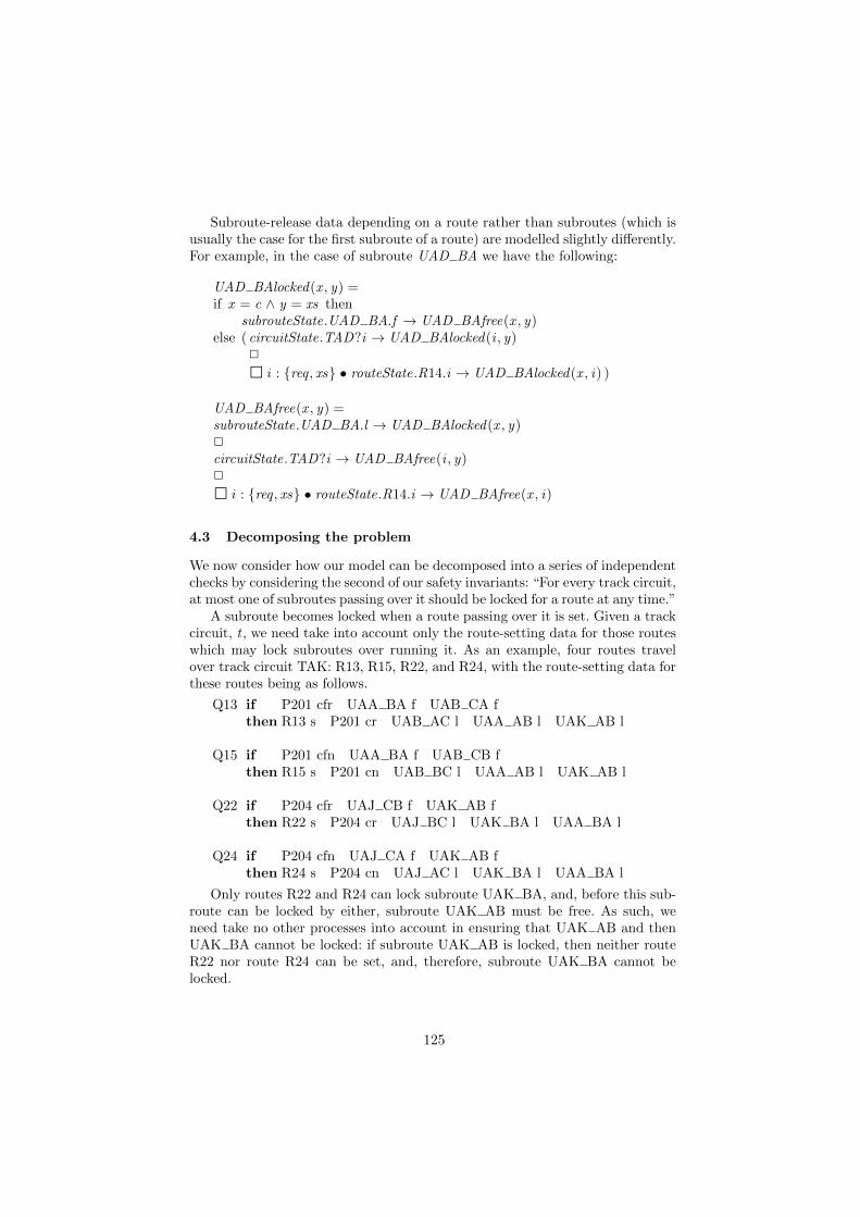
Subroute-release data depending on a route rather than subroutes (which isusually the case for the first subroute of a route) are modelled slightly differently.For example, in the case of subroute UAD BA we have the following:

UAD BAlocked(x , y) =if x = c ∧ y = xs then

subrouteState.UAD BA.f → UAD BAfree(x , y)else ( circuitState.TAD?i → UAD BAlocked(i , y)

2

2 i : {req , xs} • routeState.R14.i → UAD BAlocked(x , i) )

UAD BAfree(x , y) =subrouteState.UAD BA.l → UAD BAlocked(x , y)2

circuitState.TAD?i → UAD BAfree(i , y)2

2 i : {req , xs} • routeState.R14.i → UAD BAfree(x , i)

4.3 Decomposing the problem

We now consider how our model can be decomposed into a series of independentchecks by considering the second of our safety invariants: “For every track circuit,at most one of subroutes passing over it should be locked for a route at any time.”

A subroute becomes locked when a route passing over it is set. Given a trackcircuit, t , we need take into account only the route-setting data for those routeswhich may lock subroutes over running it. As an example, four routes travelover track circuit TAK: R13, R15, R22, and R24, with the route-setting data forthese routes being as follows.

Q13 if P201 cfr UAA BA f UAB CA fthen R13 s P201 cr UAB AC l UAA AB l UAK AB l

Q15 if P201 cfn UAA BA f UAB CB fthen R15 s P201 cn UAB BC l UAA AB l UAK AB l

Q22 if P204 cfr UAJ CB f UAK AB fthen R22 s P204 cr UAJ BC l UAK BA l UAA BA l

Q24 if P204 cfn UAJ CA f UAK AB fthen R24 s P204 cn UAJ AC l UAK BA l UAA BA l

Only routes R22 and R24 can lock subroute UAK BA, and, before this sub-route can be locked by either, subroute UAK AB must be free. As such, weneed take no other processes into account in ensuring that UAK AB and thenUAK BA cannot be locked: if subroute UAK AB is locked, then neither routeR22 nor route R24 can be set, and, therefore, subroute UAK BA cannot belocked.

125

Examining the conditions for routes R13 and R15 to be set, we see that beforeeither route can be set, subroute UAA BA must be free. The subroute-releasedata for this subroute is given by

UAA BA f if TAA c UAK BA f

It follows that we need take into account only processes representing route-setting data for routes R13 and R15, and subroute-release data for subrouteUAA BA to ensure that UAK BA and then UAK AB cannot be locked.

In this case, then, only five processes need to be considered to ensure thatsafety invariant 1 holds for track circuit TAK. The justification for this is basedupon the fact that the events with which we are concerned can only ever occurwith the co-operation of processes representing route-setting data for routesR13, R15, R22 and R24. Composition with further processes will only serve toreduce the set of possible behaviours for these components, while expanding thestate space of the check to be performed. Thus, the task of checking this safetyinvariant reduces to one of tractable size — as shown in Table 1. (Track circuitsTAE and TAF do not appear as they are both associated with exactly one route.)The automation of this dependency-establishing process is at the heart of ourapproach.

4.4 Safety invariants in CSP

We now demonstrate how we can model safety invariants. We illustrate this viathe first of our invariants: if a route is set, then all of its subroutes are locked.

For any route r , we define

U = {u : Subroute | u ∈ set(subroutesOfRoute(r))}

where set converts a sequence into a set.We represent the invariant as a process thus:

S1(r ,U , locked) =if locked = U then

2 u : locked • subrouteState.u.f → S1(r ,U , locked \ {u})2

2 routeState.r .s → routeState.r .xs → S1(r ,U , locked)

else

2 u : U \ locked • subrouteState.u.l → S1(r ,U , locked ∪ {u})2

2 u : locked • subrouteState.u.f → S1(r ,U , locked \ {u})

It is clear that we can only set a route r when all the subroutes along that routeare locked; we also require the route to become unset before any associatedsubroutes can become free.

With respect to our CSP model, we need to derive a suitable implementa-tion process, which, as per the previous subsection, involves extracting relevant

126

Track circuit States

TAA 14592TAB 3532TAC 232TAD 3312TAG 3312TAH 232TAJ 3532TAK 14592TBA 232TCA 232

Table 1. The complexity of verifying invariant 2 for our simple interlocking

process descriptions from the GDL and then combining them using parallel com-position. The following determines the necessary processes to be composed forr ∈ Route.

1. Include the processes representing route-setting data for r .2. Consider all processes related to subroute-release data for each subroute

along r , i.e. for each element in the set set(subroutesOfRoute(r)).3. The process Train(r , subroutesOfRoute(r), pointsOfRoute(r)) models a train

moving along route r .

It is the first of these steps — “include the processes representing route settingdata for r” — that allows us to decompose the checking of safety invariant 1into smaller, independent checks. Consider, for example, route R10A, where

set (subroutesOfRoute (R10A)) = {UAB CA,UBA BA}

Combining the above, we have

I1 (R10A) =R10A ‖ UAB CA ‖ UBA BA ‖ Train(R10A, 〈TAB ,TBA〉, {P201})

as the implementation process for safety invariant 1 and route R10A. Via FDR,we can verify

S1 (R10A, {UAB CA,UBA BA}, {UAB CA,UBA BA}) vF I1 (R10A)

Crucially, as all of the relevant communications are present, it follows that

S1 (R10A, {UAB CA,UBA BA}, {UAB CA,UBA BA}) vF System

By verifying similar refinements for the other routes, we can assert that safetyinvariant 1 holds for that interlocking. The proof of this relies on the fact that allrelevant behaviours relevant to the verification of the safety invariant for router can be observed in the implementation process I1 (r) (see [21]).

127

The round-trip execution times for checking each of the 16 routes of Figure 1are typically in the range 3–5 seconds; this results in a cumulative time of under 1minute to check this safety invariant for the example interlocking, which consistsof 4.84662992×1022 states;5 the cumulative times for the other safety invariantsare of a similar order.

5 Conclusions

We have described how a cloud-enabled interface for FDR gives rise to a meansof parallelized safety checks on railway interlockings. For the sake of readabil-ity, we have based our account on a relatively simple scenario; [21] shows howthe theoretical approach — which we have now made practical — is scalableto ‘real-life’ interlockings. We have concentrated on CSP and FDR, rather thanother approaches, as the relationship between parallel composition and refine-ment means that it is feasible to decompose large problems into smaller ones inan elegant fashion — making it an exceptional candidate for a cloud computingstyle approach.

One of the biggest challenges of model checking in a practical setting ishandling the enumeration of the state space in an efficient manner. Variousapproaches to alleviate the state space explosion problem are known from theliterature: partial order reduction techniques (see, for example, [22]) are one ap-proach; the local search approach proposed by Roscoe et al. [23], whereby statesspaces are partitioned into ‘blocks’, is another. An experimental parallel imple-mentation of FDR is described in [24]: states are randomly allocated betweendifferent computing nodes using a hash function; the state space is explored usinga breadth-first search algorithm, and at the end of each level successor states areexchanged between the compute nodes. An alternative approach is that taken byFDR Explorer [25], whereby an API “makes possible to create optimised CSPcode to perform refinement checks that are more space or time efficient, enablingthe analysis of more complex and data-intensive specifications.”

Our approach involves partitioning the problem not at the level of the statespace, but at the level of the CSP model — which means it is applicable onlyin certain contexts, with one being the scenario considered in this paper. Allof the refinement checks are generated automatically and subsequently sent toslave nodes for processing. There are clearly limitations, though. Crucially, werely upon the existence of models being of a form that can be decomposed intosmaller subproblems; once this partitioning is done, the refinement checks canthen be allocated to a farm of processors to either be confirmed or refuted. Whiledeconstructing the problem at the model level in the way that we have done canwork for safety properties, it is of no use when considering liveness properties,for example.

The initial prototype implementation of the software that schedules thechecks between processing nodes can be extended in several ways. At the mo-

5 12 track circuits, 4 points, 16 routes and 30 subroutes, giving rise to 212×44×316×230

states.

128

ment, there is a single point of failure: should the master node die, there wouldbe no way to schedule more refinement checks or to collect the results. Anotherpoint to consider would be the costing model used by the cloud provider: giventhat virtual instances are priced per hour, if many of the refinement checks aresimilar (as per the case study of this paper), we can try and optimise the costby considering the execution time of a single check. The most pressing item offuture work, however, is the consideration of further case studies — with a viewto identifying other classes of problems that may benefit from this approach.Initial ares of interest in this respect are asynchronous hardware circuits andautomatic test case generation.

Acknowledgements

The authors would like to thank the anonymous reviewers for their helpful com-ments and constructive criticisms.

References

1. Hansen, K.M.: Validation of a railway interlocking model. In Naftalin, M., Denvir,T., Bertran, M., eds.: Proceedings of the 2nd International Symposium of FormalMethods Europe (FME 1994). Volume 873 of Lecture Notes in Computer Science.Springer (1994) 582–601

2. Morley, M.J.: Safety in railway signalling data: a behavioural analysis. In Joyce,J., Seger, C., eds.: Proceedings of the 6th Annual Workshop on Higher Order Logicand its Applications. Volume 780 of Lecture Notes in Computer Science. Springer(1994) 465–474

3. Haxthausen, A.E., Peleska, J.: Formal development and verification of a distributedrailway control system. IEEE Transaction on Software Engineering 26(8) (2000)687–701

4. Kanso, K., Moller, F., Setzer, A.: Automated verification of signalling principlesin railway interlocking systems. Electronic Notes in Theoretical Computer Science250(2) (2009) 19–31

5. James, P., Roggenbach, M.: Automatically verifying railway interlockings usingSAT-based model checking. In: Proceedings of the 10th International Workshopon Automated Verification of Critical Systems (AVoCS 2010), Electronic Commu-nication of the European Association of Software Science and Technology volume35 (2010)

6. Haxthausen, A.E., Peleska, J., Kinder, S.: A formal approach for the constructionand verification of railway control systems. Formal Aspects of Computing 23(2)(2011) 191–219

7. Fantechi, A., Fokkink, W., Morzenti, A.: Some trends in formal methods applica-tions to railway signalling. In Gnesi, S., Margaria, T., eds.: Formal Methods forIndustrial Critical Systems: A Survey of Applications. John Wiley & Sons (2013)63–82

8. Bacherini, S., Fantechi, A., Tempestini, M., Zingoni, N.: A story about formalmethods adoption by a railway signaling manfacturer. In Misra, J., Nipkow, T.,Sekerinski, E., eds.: Proceedings of the 14th International Symposium on FormalMethods (FM 2006). Volume 4085 of Lecture Notes in Computer Science. Springer(2006) 179–189

129

9. Winter, K., Robinson, N.J.: Modelling large interlocking systems and model check-ing small ones. In Oudshoorn, M., ed.: Proceedings of the 26th Australasian Com-puter Science Conference (ACSC 2003), Australian Computer Science Communi-cations volume 16 (2003) 309–316

10. Simpson, A.C., Woodcock, J.C.P., Davies, J.W.M.: The mechanical verification ofSolid State Interlocking geographic data. In Groves, L., Reeves, S., eds.: Proceed-ings of Formal Methods Pacific 1997. Springer (1997) 223–242

11. Hoare, C.A.R.: Communicating Sequential Processes. Prentice Hall (1985)12. Roscoe, A.W.: Understanding Concurrent Systems. Springer-Verlag (2010)13. Roscoe, A.W.: Model checking CSP. In Roscoe, A.W., ed.: A Classical Mind:

Essays in Honour of C. A. R. Hoare. Prentice Hall (1994)14. Roscoe, A.W., Gardiner, P.H.B., Goldsmith, M.H., Hulance, J.R., Jackson, D.M.,

Scattergood, J.B.: Hierarchical compression for model-checking CSP or how tocheck 1020 dining philosophers for deadlock. In: Proceedings of the First Inter-national Workshop on Tools and Algorithms for the Construction and Analysisof Systems (TACAS 1995). Volume 1019 of Lecture Notes in Computer Science.Springer (1995) 133–152

15. Nurmi, D., Wolski, R., Grzegorczyk, C., Obertelli, G., Soman, S., Youseff, L.,Zagorodnov, D.: The Eucalyptus open-source cloud-computing system. In: Pro-ceedings of the 9th IEEE/ACM International Symposium on Cluster Computingand the Grid (CCGRID 2009). (2009) 124–131

16. Brookes, S.D., Roscoe, A.W.: An improved failures model for communicatingprocesses. In Brookes, S.D., Roscoe, A.W., Winskel, G., eds.: Proceedings of theNSF-SERC Seminar on Concurrency. Volume 197 of Lecture Notes in ComputerScience. Springer (1985) 281–305

17. Roscoe, A.W.: The Theory and Practice of Concurrency. Prentice Hall (1997)18. Ferrari, A., Magnani, G., Grasso, D., Fantechi, A.: Model checking interlocking

control tables. In: Proceedings of Formal Methods for Automation and Safetyin Railway and Automotive Systems 2010 (FORMS/FORMAT 2010). Springer(2011) 107–115

19. Cribbens, A.: Solid State Interlocking (SSI): An integrated electronic signallingsystem for mainline railways. IEE Proceedings 134(3) (1987) 148–158

20. British Rail Research: SSI data preparation guide. Published by British RailwaysBoard. ELS-DOC-3080, Issue K of SSI8003-INT and supplements (1990)

21. Simpson, A.C.: Safety through security. DPhil thesis, Oxford University Comput-ing Laboratory (1996)

22. Godefroid, P.: Partial-Order Methods for the Verification of Concurrent Systems:An Approach to the State-Explosion Problem. Springer-Verlag (1996)

23. Roscoe, A.W., Armstrong, P.J., Pragyesh: Local search in model checking. In:Proceedings of the 7th International Symposium on Automated Technology forVerification and Analysis (ATVA 2009). Volume 5799 of Lecture Notes in ComputerScience., Springer (2009) 22–38

24. Goldsmith, M.H., Martin, J.M.R.: The parallelisation of FDR. In: Proceedings ofWorkshop on Parallel and Distributed Model Checking (PDMC 2002). (2002)

25. Freitas, L., Woodcock, J.C.P.: FDR Explorer. Formal Aspects of Computing21(1–2) (2009) 133–154

130

Counterexample Generation forHybrid Automata

Johanna Nellen1, Erika Abraham1, Xin Chen1, and Pieter Collins2

1 RWTH Aachen University, Germany2 Maastricht University, The Netherlands

Abstract. The last decade brought us a whole range of over-approxima-tive algorithms for the reachability analysis of hybrid automata, a widelyused modeling language for systems with combined discrete-continuousbehavior. Besides theoretical results, there are also some tools availablefor proving safety in the continuous time domain. However, if a givenset of critical states is found to be reachable, these tools do not providecounterexamples for models beyond timed automata.This paper investigates the question whether and how available toolscan be used to generate counterexamples, even if this functionality isnot directly supported. Using the tools SpaceEx and Flow*, we discusspossibilities to solve our task with and without modifying the tools’source code, report on the effort and the efficiency of implementation, andpropose a simulation-based approach for the validation of the resulting(possibly spurious) counterexamples.

1 Introduction

Hybrid systems are systems that exhibit both continuous and discrete behavior.Typical examples are physical systems regulated by discrete controllers, e.g., au-tomotive control systems or controlled chemical plants. Hybrid systems are oftenmodeled as hybrid automata [1], for which the reachability problem is undecid-able. Despite undecidability and driven by the fact that most hybrid systemsin industrial context are safety-critical, a lot of effort was put into the devel-opment of reachability analysis techniques for hybrid automata. State-of-the-arttools like SpaceEx [2] and Flow* [3] try to compute an over-approximation ofthe reachable state space and can therefore be used to prove safety, i.e., thata given set of unsafe states cannot be reached from a set of initial states in agiven model. However, if the over-approximation of the reachable states containsunsafe states then no conclusive answer can be given.

Counterexamples in form of system runs leading to unsafe states would beextremely valuable, even if they are spurious, i.e., if they were considered in theanalysis but are not possible in the given model. For safe models they couldhelp to reduce the approximation error in the analysis efficiently, whereas forunsafe models they could provide important information about the source ofthe critical system behavior. Counterexamples would enable the application of

131

counterexample-guided abstraction refinement (CEGAR) techniques and couldalso play an important role in controller synthesis.

Unfortunately, none of the available tools for hybrid automata reachabilityanalysis with continuous time domain computes counterexamples. It is surprisingsince internally they possess sufficient information to generate at least a coarseover-approximation of a counterexample in form of a sequence of jumps (i.e.,changes in the discrete part of the system state), augmented with time intervalsover-approximating the time durations between the jumps. In this paper we

1. examine whether it is possible to either use augmented system models or toextract information from the output of the SpaceEx tool such that we cansynthesize over-approximations of counterexamples;

2. study how the efficiency can be improved by extending the functionality ofthe Flow* tool internally, i.e., by making modifications to the source code;

3. develop a simulation-based approach to validate the counterexample over-approximations, i.e., to determine unsafe paths in the over-approximation.

We have chosen SpaceEx and Flow* for our experiments because on the onehand SpaceEx is one of the most popular hybrid automata reachability analysistools and on the other hand some of the authors belong to the implementationteam of Flow*, i.e., the modification of the source code of Flow* could bedone safely. Unfortunately, counterexample generation without tool extension isunsatisfactory: we need either expensive additional analysis runs for enlargedsystems or parsing hidden information from debug output. The results demon-strate the need to extend the functionality of available analysis tools to gener-ate counterexamples internally. However, even if that task is done, the resultsstrongly over-approximate counterexamples, whose existence can be indicatedbut not proven. Thus we need novel methods to refine and validate the results,posing highly challenging problems in both theory and practice.

Related work In this paper we focus on reachability analysis techniques forcontinuous-time hybrid automata that apply a fixed-point-based forward-reach-ability iteration [1]. Such algorithms need two main ingredients: (a) A tech-nique to represent state sets and to compute certain operations on them likeunion, intersection, Minkowski sum, etc. All the available tools work with over-approximative representations and computations. Popular approaches use eithergeometric objects like hyperrectangles [4], polyhedra [5–9], zonotopes [10, 11],orthogonal polyhedra [12] or ellipsoids [13], or symbolic representations like sup-port functions [14, 15] or Taylor models [16, 17]. The choice of the representationis crucial, as it strongly influences the approximation error and the efficiencyof the computations. (b) A method to compute one-step-successors of state setsboth for continuous flow and discrete jumps. A flowpipe is an over-approximationof the states that are reachable from a given initial set of states by letting timeprogress within a certain maximal time horizon. To compute a flowpipe, themaximal time horizon is often divided into smaller intervals and the flowpipe isrepresented as a (finite) union of state sets (flowpipe segments), each coveringone of the smaller intervals [5].

132

The analysis tools HyTech [6], PHAVer [7] and the Multi-Parametric Tool-box [8] use convex polyhedra for the over-approximative representation of statesets, SpaceEx [2] additionally allows the usage of support functions. In [18], thestate sets are over-approximated by level sets. The tool d/dt [19] uses grid pavingas over-approximations. MATISSE [20] over-approximates state sets by zono-topes. The MATLAB Ellipsoidal Toolbox [21] supports the over-approximativerepresentation of sets by ellipsoids, Flow* by Taylor models. In Ariadne [22],the state sets may be over-approximated by Taylor models or grid pavings. Incontrast to the other tools, Flow*, HyTech, PHAVer, Ariadne and d/dt alsosupport the analysis of non-linear hybrid automata (with non-linear differentialequations).

None of these tools supports the generation of counterexamples. There aresome works [23, 24] related to counterexample generation for hybrid systems, butthey are mostly devoted to CEGAR approaches for restricted classes of hybridautomata like, e.g., (initialized) rectangular automata.

Outline After some preliminaries in Section 2, we describe in the Sections 3and 4 how we can compute over-approximations of counterexamples for unsafemodels, whose validation is discussed in Section 5. Section 6 concludes the paper.

2 Preliminaries

ont = 1t ≤ 22

offt = −0.5t ≥ 18

t ≥ 21

t ≤ 19

t = 20

Fig. 1. The thermostat example

By N, Z and R we denote the set of all natu-ral (with 0), integer and real numbers, respec-tively, by R≥0 the non-negative reals, and useN>0 = N\{0}. For some n ∈ N>0, let Var ={x1, . . ., xn} be an ordered set of variables overR. We use the notation x = (x1, . . ., xn), anddenote by Var ′ and ˙Var the renamed vari-able sets {x′1, . . ., x′n} and {x1, . . ., xn}, respec-tively. Given a real-arithmetic formula φ overVar, its satisfaction set is JφK = {v ∈ Rn | φ[v/x] = true}; we call φ convex if JφKis convex. Let Φ(Var) be the set of all quantifier-free convex real-arithmetic for-mulas (so-called predicates) over Var. A predicate is linear if it can be expressedin linear real arithmetic.

Definition 1 (Syntax of hybrid automata). A hybrid automaton (HA)is a tuple H = (Loc,Var,Edge,Dyn, Inv, Init) with the following components:

– Loc is a finite set of locations or modes.– Var = {x1, . . ., xn} is a finite ordered set of variables over R. A valuation v =

(v1, . . ., vn) ∈ Rn defines for each i = 1, . . ., n the value vi for xi. A state is amode-valuation pair σ = (l, v) ∈ Loc× Rn = Σ.

– Edge ⊆ Loc×Φ(Var∪Var ′)×Loc is a finite set of edges. For an edge e = (l, φ, l′) ∈Edge we call l (l′) the source (target) mode of e and φ its transition relation.

– Dyn : Loc→ Φ(Var ∪ ˙Var) assigns a dynamics to each mode.– Inv : Loc→ Φ(Var) assigns an invariant to each mode.– Init : Loc→ Φ(Var) specifies the initial valuations for each mode.

133

(x1x2

)=

(v1v2

)and

(v1v2

)=

(−1.8 −0.2−0.2 −1.8

)(v1v2

)+

(b1b2

)in each location

with b1, b2 as specified inside the location, c = 0.7017

`1b1 = 1 b2 = 0x1 ∈ [0, 1]∧x2 ∈ [0, 1]

`2b1 = −1 b2 = 0x1 ∈ [2, 3]∧x2 ∈ [0, 1]

`3b1 = −1 b2 = 0x1 ∈ [3, 4]∧x2 ∈ [0, 1]

`4b1 = 0 b2 = 1x1 ∈ [0, 1]∧x2 ∈ [1, 2]

`5b1 = −c b2 = cx1 ∈ [1, 2]∧x2 ∈ [1, 2]

`6b1 = −c b2 = −c

x1 ∈ [2, 3]∧x2 ∈ [1, 2]

`7b1 = −c b2 = −c

x1 ∈ [3, 4]∧x2 ∈ [1, 2]

`8b1 = −1 b2 = 0x1 ∈ [1, 2]∧x2 ∈ [2, 3]

`9b1 = 0 b2 = −1x1 ∈ [2, 3]∧x2 ∈ [2, 3]

`10b1 = 0 b2 = −1x1 ∈ [3, 4]∧x2 ∈ [2, 3]

`11b1 = 0 b2 = −1x1 ∈ [0, 1]∧x2 ∈ [3, 4]

`12b1 = −1 b2 = 0x1 ∈ [1, 2]∧x2 ∈ [3, 4]

`13b1 = 0 b2 = −1x1 ∈ [2, 3]∧x2 ∈ [3, 4]

`14b1 = 0 b2 = −1x1 ∈ [3, 4]∧x2 ∈ [3, 4]

x1 ∈ [3, 3.8],x2 ∈ [3, 4],v1 ∈ [−0.1, 0.1],v2 ∈ [−0.8,−0.5]

x1 = 3∧v1 ≥ 0

x1 = 1∧v1 ≥ 0

x1 = 2∧v1 ≥ 0

x1 = 3∧v1 ≥ 0

x1 = 2∧v1 ≥ 0

x1 = 3∧v1 ≥ 0

x1 = 1∧v1 ≥ 0

x1 = 2∧v1 ≥ 0

x1 = 3∧v1 ≥ 0

x1 = 3∧v1 ≤ 0

x1 = 1∧v1 ≤ 0

x1 = 2∧v1 ≤ 0

x1 = 3∧v1 ≤ 0

x1 = 2∧v1 ≤ 0

x1 = 3∧v1 ≤ 0

x1 = 1∧v1 ≤ 0

x1 = 2∧v1 ≤ 0

x1 = 3∧v1 ≤ 0

x2 = 3∧v2 ≤ 0

x2 = 3∧v2 ≤ 0

x2 = 3∧v2 ≤ 0

x2 = 2∧v2 ≤ 0

x2 = 2∧v2 ≤ 0

x2 = 2∧v2 ≤ 0

x2 = 1∧v2 ≤ 0

x2 = 1∧v2 ≤ 0

x2 = 1∧v2 ≤ 0

x2 = 3∧v2 ≥ 0

x2 = 3∧v2 ≥ 0

x2 = 3∧v2 ≥ 0

x2 = 2∧v2 ≥ 0

x2 = 2∧v2 ≥ 0

x2 = 2∧v2 ≥ 0

x2 = 1∧v2 ≥ 0

x2 = 1∧v2 ≥ 0

x2 = 1∧v2 ≥ 0

Fig. 2. The navigation benchmark

Since we do not use the parallel composition of hybrid automata in this paper,for simplicity we skipped composition-relevant parts in the above definition.

A toy example of a thermostat is depicted graphically in Figure 1. The rect-angles represent modes; their names, dynamics and invariants are specified insidethe rectangle. Initial valuations are specified on an incoming edge of a given modewithout a source mode; a missing incoming edge stays for the initial conditionfalse. Figure 2 shows the navigation benchmark [25], which we use later on forexperiments. It models an object moving in the R2 plane. The velocity (v1, v2)of the object depends on its position (x1, x2) in a grid. For some experiments weadd a parameter ε to the navigation benchmark to enlarge the satisfaction setsof guards and invariants by replacing all upper bounds ub (lower bounds lb) byub + ε (lb− ε).

Definition 2 (Semantics of hybrid automata). The operational semanticsof a HA H = (Loc,Var,Edge,Dyn, Inv, Init) with Var = {x1, . . ., xn} is given bythe rules of Figure 3. The first rule specifies time evolution (time steps), thesecond one discrete mode changes (jumps).

134

l ∈ Loc v, v′ ∈ Rn t ∈ R≥0 f : [0, t]→ Rndifferentiable f = dfdt

f(0) = v f(t) = v′ ∀t′ ∈ [0, t]. f(t′) ∈ JInv(l)K ∧ (f(t′), f(t′)) ∈ JDyn(l)KTime

(l, v)t→ (l, v′)

l, l′ ∈ Loc v, v′ ∈ Rn v ∈ JInv(l)K v′ ∈ JInv(l′)K e = (l, φ, l′) ∈ Edge (v, v′) ∈ JφKJump

(l, v)e→ (l′, v′)

Fig. 3. Operational semantics rules for hybrid automata

Let →=⋃

t∈R≥0

t→ ∪⋃e∈Edgee→. A path of H is a (finite or infinite) se-

quence (l0, v0) → (l1, v1) → . . .. For an initial path we additionally requirev0 ∈ JInit(l0)K. A state (l, v) ∈ Σ is called reachable in H if there is an initialpath (l0, v0)→ (l1, v1)→ . . . of H and an index i ≥ 0 such that (li, vi) = (l, v).

Please note that each reachable state (l, v) of H can be reached via an initial

path of H of the form (l0, v0)t0→ (l0, v

′0)

e0→ . . .(ln−1, vn−1)tn−1→ (ln−1, v′n−1)

en−1→(ln, vn)

tn→ (ln, v′n) = (l, v) with alternating time steps and jumps for some n ∈ N.

In the following we consider only paths of this form.A trace e0, e1, . . . describes a sequence of jumps with ei ∈ Edge such that the

target mode of ei equals the source mode of ei+1 for all i ∈ N. If we can assumethat there is at most one jump between each mode pair, we also identify tracesby the sequence l0, l1, . . . of modes visited. Such a trace represents the set of all

paths (l0, v0)t′′0→ (l0, v

′0)

e0→ (l1, v1)t′′1→ (l1, v

′1)

e1→ . . .. We say that those paths arecontained in the symbolic path.

A timed trace e0, [t0, t′0], e1, [t1, t

′1], . . . annotates a trace e0, e1, . . . with time

intervals and represents the set of all paths (l0, v0)t′′0→ (l0, v

′0)

e0→ (l1, v1)t′′1→

(l1, v′1)

e1→ . . . with t′′i ∈ [ti, t′i] for all i ∈ N. We say that e0, [t0, t

′0], e1, [t1, t

′1], . . .

is a timed trace of the represented paths, which are contained in the timed trace.Given a HA H and a set B of unsafe states of H, the reachability problem

poses the question whether the intersection of B with the reachable state setof H is empty, i.e., whether H is safe. If H is unsafe, a counterexample is aninitial path of H leading to an unsafe state from B. For models with weakerexpressivity, for example hybrid automata defined by linear predicates and con-stant derivatives (i.e., dynamics of the form

∧x∈Var x = cx with cx ∈ Z for all

x ∈Var), the bounded reachability problem is decidable and, for unsafe models,counterexamples can be generated (e.g., by bounded model checking using SMTsolving with exact arithmetic). However, the computation of counterexamplesfor general hybrid automata is hard. Theoretically, it could be done by (incom-plete) under-approximative reachability computations, but currently there areno techniques available for this task.

In this paper we propose an approach to generate and refine presumablecounterexamples, which are timed traces that might contain a counterexample;if a presumable counterexample does not contain any counterexample then wesay that it is spurious.

135

3 Generating Traces for Presumable Counterexamples

Existing hybrid automata analysis tools like SpaceEx offer as output optionseither the computed over-approximation of the reachable state space, its in-tersection with the unsafe states, or just the answer whether unsafe states arereachable or not (in the over-approximation). However, in contrast to tools fordiscrete automata, none of the tools for hybrid automata provides counterexam-ples.

In this section we show how a trace explaining the reachability of unsafe statescan be computed. We present three different approaches: The first approach aug-ments hybrid automata with auxiliary variables to make observations about thecomputation history of the analysis. The second approach can be used if theanalysis tool outputs sufficient information about the paths that have been pro-cessed during the analysis. The third approach suggests to implement some newfunctionalities efficiently in existing tools. In our experiments we used SpaceExv0.9.7c, VMware server, and the latest Flow* version but with the proposedextensions.

3.1 Approach I: Model Augmentation

We extend the model with new variables to make book-keeping about tracesthat lead to unsafe states in the reachability analysis. First we augment themodel and analyze the augmented system to observe the number of jumps untilan unsafe state is reached. Then we augment and analyze an unrolled model toobserve unsafe traces.

Determining the counterexample length We augment the model and analyze it togain information about the length of paths leading to unsafe states. We introducea counter tr with initial value 0, define tr=0 in each mode, and let each jumpincrease the counter value by one.

However, the unboundedness of tr would render the fixed-point analysis tobe non-terminating. To bound tr from above, we define a constant maxtr andeither extend the invariants or the edge guards to forbid higher values.

The value of maxtr should be guessed, and in case the analysis of the aug-mented model reports safety, increased. A possible guess could be the number ofiterations during the fixed-point analysis of the original model, which is reportedby SpaceEx and specifies how many times the tool computed a (time+jump) suc-cessor of a state set. To get a smaller value (and thus shorter counterexampleswith less computational effort), the reachability analysis could be stopped whenan unsafe state is reached. Unfortunately, SpaceEx does not offer this option.

Definition 3 (Guard and invariant augmentation). Let H = (Loc,Var,Edge, Dyn, Inv, Init) be a HA and maxtr ∈ N. The guard augmentation of H isthe HA Hguard = (Loc,Var ∪ {tr},Edge′,Dyn′, Inv, Init ′) with

– Edge′ = {(l, (φ ∧ tr ≤ maxtr − 1 ∧ tr′=tr+1), l′) | (l, φ, l′) ∈ Edge};– Dyn′(l) = (Dyn(l) ∧ tr=0) for each l ∈ Loc;– Init ′(l) = (Init(l) ∧ tr=0) for each l ∈ Loc.

136

ont=1 ∧ tr=0

t≤22

offt=− 0.5 ∧ tr=0

t≥18

t≥21 ∧ tr≤maxtr−1 ∧ tr′=tr+1

t≤19 ∧ tr≤maxtr−1 ∧ tr′=tr+1t=20∧tr=0

ont=1 ∧ tr=0

t≤22 ∧ tr≤maxtr

offt=− 0.5 ∧ tr=0t≥18 ∧ tr≤maxtr

t≥21 ∧ tr′=tr+1

t≤19 ∧ tr′=tr+1t=20∧tr=0

Fig. 4. The guard (left) and the invariant (right) augmentation of the thermostat model

The invariant augmentation of H is the HA Hinv = (Loc,Var ∪ {tr},Edge′′,Dyn′, Inv ′′, Init ′) with Dyn′ and Init ′ as above and

– Edge′′ = {(l, (φ ∧ tr′=tr+1), l′) | (l, φ, l′) ∈ Edge};– Inv ′′(l) = (Inv(l) ∧ tr ≤ maxtr) for each l ∈ Loc.

Figure 4 illustrates the augmentation on the thermostat example. Note that,apart from restricting the number of jumps, the above augmentation does notmodify the original system behavior. The size of the state space is increasedby the factor maxtr+1, since the value domain of tr is [0,maxtr] ⊆ N for theconstant maxtr.

When we analyze the augmented model, SpaceEx returns for each mode inthe over-approximated set of reachable unsafe states an over-approximation [l, u]for the values of tr.

Since tr takes integer values only, the lower and upper bounds are not ap-proximated, i.e., during analysis both after l and after u (over-approximative)jump computations unsafe states were reached, but we do not have any infor-mation about the values inbetween. Therefore we fix the number k, describingthe length of counterexamples we want to generate, to be either l or u.

We made some experiments for the thermostat example with unsafe states t ≤19, and for the navigation benchmark with unsafe states (x1, x2) ∈ [1, 2]× [0, 1].Table 1 compares for different maxtr values the number of SpaceEx iterations, therunning times, and the resulting tr values for the original models, the guard andthe invariant augmentations. For the same number of iterations, the augmentedmodels need in average some more (but still comparable) time for the analysisthan the original models; the invariant and guard augmentations seem to besimilar in terms of running time.

Trace encoding In order to observe the traces leading to unsafe states, we needto remember the jumps in the order of their occurrences. We achieve this byunrolling the transition relation of the original model k times, where k is thecounterexample length determined in the previous step.

We could define the unrolling by copying each mode k + 1 and each edge ktimes, and let the ith copy of an edge connect the ith-copy of the source modewith the (i + 1)st copy of the target mode. To remember the jumps taken, weintroduce k auxiliary variables tr1, . . ., trk and store on the ith copy of an edgethe edge’s identity in tri. Such an unrolling would cause a polynomial increasein the size of the model.

137

Table 1. Evaluation of the guard and invariant augmentations with a sampling timeof 0.1 and a time horizon of 30

model augment. maxtr #iter. fixed point running time [secs] tr

thermostat none - 5/11/31 no/no/no 0.11/0.24/0.69 -example guard 4/10/30 5/11/31 yes/yes/yes 0.25/0.65/2.15 [1, 4]/[1, 10]/[1, 30]

invar. 4/10/30 5/11/31 yes/yes/yes 0.30/0.78/2.53 [1, 4]/[1, 10]/[1, 30]

navigation none - 29/168/3645 no/no/no 1.54/8.63/1598.63 -benchmark guard 4/10/30 29/168/3645 yes/yes/yes 1.92/12.25/2088.88 [4, 4]/[4, 10]/[4, 30]

invar. 4/10/30 29/168/3160 yes/yes/yes 2.06/13.02/1466.08 [4, 4]/[4, 10]/[4, 30]

navigation2 none - 32/524 no/no 7.55/254.91 -benchmark, guard 4/10 32/524 yes/yes 7.55/284.19 [4, 4]/[4, 10]ε = 0.1 invar. 4/10 32/524 yes/yes 7.35/293.88 [4, 4]/[4, 10]

However, in such an unrolling there might be different traces leading to thesame mode. SpaceEx would over-approximate these trace sets by a mode-wiseclosure, such that we cannot extract them from the result. E.g., for two tracesl1, l2, l4, l5, l7 and l1, l3, l4, l6, l7, resp., also the trace l1, l2, l4, l6, l7 would be in-cluded in the over-approximation. Therefore, we copy each mode as many timesas the number of different traces of length up to k leading to it. This yields anexponential growth in k for the number of locations and transitions.

We augment the unrolled model to observe the traces to unsafe states. In anaive encoding, we identify edges e1, . . ., ed by numbers 1, . . ., d, and introducenew variables tri for i=1, . . ., k to store the edges taken.

We also define an advanced encoding which needs less auxiliary variables. Ifthe domain of a variable includes [0, |Edge|n] for some n ∈ N then we can useit to store a sequence of n edges: Each time an edge is taken, we multiply thecurrent value by |Edge| and add the identity of the taken edge. This way we need⌈kn

⌉auxiliary variables to encode a path of length k.

Definition 4 (k-unrolling, trace encoding). Assume a HA H = (Loc,Var,Edge,Dyn, Inv, Init) with an ordered set {e1, . . ., ed} of edges. The k-unrolling ofH is the HA Hu = (Locu,Varu,Edgeu,Dynu, Invu, Initu) with

– Locu =⋃

i=1,...,k+1 Loci;– Varu =Var;– Edgeu = {((l1, . . ., li), φ, (l1, . . ., li, li+1)) | 1 ≤ i ≤ k ∧ (li, φ, li+1) ∈ Edge};– Dynu(l1, . . ., li) = Dyn(li) for all (l1, . . ., li) ∈ Locu;– Invu(l1, . . ., li) = Inv(li) for all (l1, . . ., li) ∈ Locu;– Initu(l1, . . ., li) = Init(li) for i = 1 and false otherwise, for all (l1, . . ., li) ∈ Locu.

The naive trace encoding of H with depth k is the HA H1 = (Locu,Var1,Edge1,Dyn1, Invu, Init1) with

– Var1 =Var ∪ {tr1, . . ., trk};– Edge1 = {((l1, . . ., li), φ ∧ tr′i=j, (l1, . . ., li, li+1)) | 1 ≤ i ≤ k ∧ ej=(li, φ, li+1) ∈ Edge};– Dyn1(l1, . . ., li) = Dynu(l1, . . ., li) ∧

∧kj=1 trj = 0 for all (l1, . . ., li) ∈ Locu;

– Init1(l1, . . ., li) = Initu(l1, . . ., li) ∧∧k

j=1 trj = 0 for all (l1, . . ., li) ∈ Locu.

Let n ∈ N>0 such that [0, dn] is included in the domain of each tri and letz=d kne. The advanced trace encoding of H with depth k is the HA H2 =

138

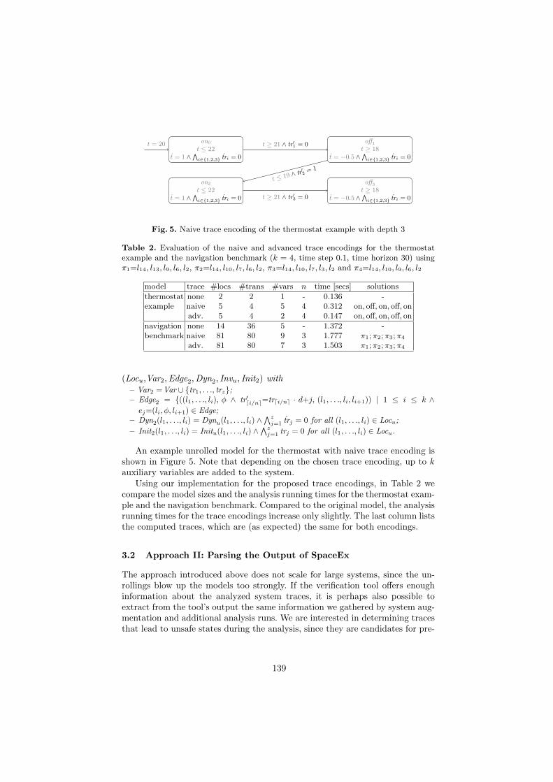
on0

t ≤ 22t = 1 ∧∧

i∈{1,2,3} tri = 0

off1

t ≥ 18t = −0.5 ∧∧

i∈{1,2,3} tri = 0

on2

t ≤ 22t = 1 ∧∧

i∈{1,2,3} tri = 0

off3

t ≥ 18t = −0.5 ∧∧

i∈{1,2,3} tri = 0

t ≥ 21 ∧ tr′1 = 0

t ≤ 19 ∧ tr′2

= 1

t ≥ 21 ∧ tr′3 = 0

t = 20

Fig. 5. Naive trace encoding of the thermostat example with depth 3

Table 2. Evaluation of the naive and advanced trace encodings for the thermostatexample and the navigation benchmark (k = 4, time step 0.1, time horizon 30) usingπ1=l14, l13, l9, l6, l2, π2=l14, l10, l7, l6, l2, π3=l14, l10, l7, l3, l2 and π4=l14, l10, l9, l6, l2

model trace #locs #trans #vars n time [secs] solutions

thermostat none 2 2 1 - 0.136 -example naive 5 4 5 4 0.312 on, off, on, off, on

adv. 5 4 2 4 0.147 on, off, on, off, on

navigation none 14 36 5 - 1.372 -benchmark naive 81 80 9 3 1.777 π1;π2;π3;π4

adv. 81 80 7 3 1.503 π1;π2;π3;π4

(Locu,Var2,Edge2,Dyn2, Invu, Init2) with– Var2 =Var ∪ {tr1, . . ., trz};– Edge2 = {((l1, . . ., li), φ ∧ tr′di/ne=trdi/ne · d+j, (l1, . . ., li, li+1)) | 1 ≤ i ≤ k ∧ej=(li, φ, li+1) ∈ Edge;

– Dyn2(l1, . . ., li) = Dynu(l1, . . ., li) ∧∧z

j=1 trj = 0 for all (l1, . . ., li) ∈ Locu;

– Init2(l1, . . ., li) = Initu(l1, . . ., li) ∧∧z

j=1 trj = 0 for all (l1, . . ., li) ∈ Locu.

An example unrolled model for the thermostat with naive trace encoding isshown in Figure 5. Note that depending on the chosen trace encoding, up to kauxiliary variables are added to the system.

Using our implementation for the proposed trace encodings, in Table 2 wecompare the model sizes and the analysis running times for the thermostat exam-ple and the navigation benchmark. Compared to the original model, the analysisrunning times for the trace encodings increase only slightly. The last column liststhe computed traces, which are (as expected) the same for both encodings.

3.2 Approach II: Parsing the Output of SpaceEx

The approach introduced above does not scale for large systems, since the un-rollings blow up the models too strongly. If the verification tool offers enoughinformation about the analyzed system traces, it is perhaps also possible toextract from the tool’s output the same information we gathered by system aug-mentation and additional analysis runs. We are interested in determining tracesthat lead to unsafe states during the analysis, since they are candidates for pre-

139

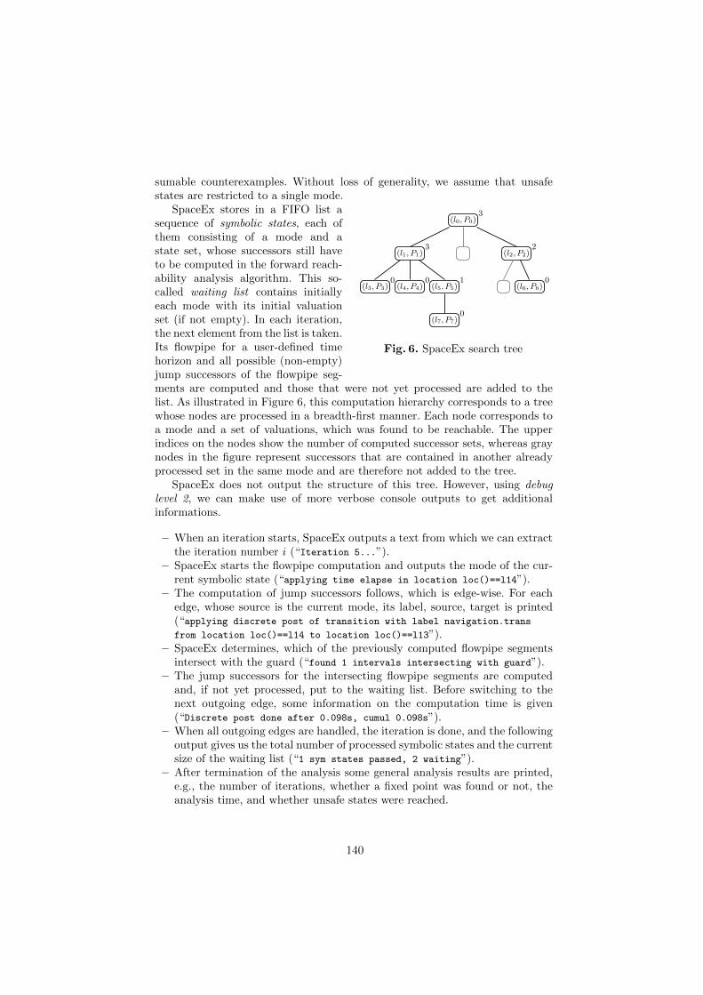
sumable counterexamples. Without loss of generality, we assume that unsafestates are restricted to a single mode.

(l0, P0)3

(l1, P1)3

(l2, P2)2

(l4, P4)0

(l3, P3)0

(l5, P5)1

(l6, P6)0

(l7, P7)0

Fig. 6. SpaceEx search tree

SpaceEx stores in a FIFO list asequence of symbolic states, each ofthem consisting of a mode and astate set, whose successors still haveto be computed in the forward reach-ability analysis algorithm. This so-called waiting list contains initiallyeach mode with its initial valuationset (if not empty). In each iteration,the next element from the list is taken.Its flowpipe for a user-defined timehorizon and all possible (non-empty)jump successors of the flowpipe seg-ments are computed and those that were not yet processed are added to thelist. As illustrated in Figure 6, this computation hierarchy corresponds to a treewhose nodes are processed in a breadth-first manner. Each node corresponds toa mode and a set of valuations, which was found to be reachable. The upperindices on the nodes show the number of computed successor sets, whereas graynodes in the figure represent successors that are contained in another alreadyprocessed set in the same mode and are therefore not added to the tree.

SpaceEx does not output the structure of this tree. However, using debuglevel 2, we can make use of more verbose console outputs to get additionalinformations.

– When an iteration starts, SpaceEx outputs a text from which we can extractthe iteration number i (“Iteration 5...”).

– SpaceEx starts the flowpipe computation and outputs the mode of the cur-rent symbolic state (“applying time elapse in location loc()==l14”).

– The computation of jump successors follows, which is edge-wise. For eachedge, whose source is the current mode, its label, source, target is printed(“applying discrete post of transition with label navigation.trans

from location loc()==l14 to location loc()==l13”).– SpaceEx determines, which of the previously computed flowpipe segments

intersect with the guard (“found 1 intervals intersecting with guard”).– The jump successors for the intersecting flowpipe segments are computed

and, if not yet processed, put to the waiting list. Before switching to thenext outgoing edge, some information on the computation time is given(“Discrete post done after 0.098s, cumul 0.098s”).

– When all outgoing edges are handled, the iteration is done, and the followingoutput gives us the total number of processed symbolic states and the currentsize of the waiting list (“1 sym states passed, 2 waiting”).

– After termination of the analysis some general analysis results are printed,e.g., the number of iterations, whether a fixed point was found or not, theanalysis time, and whether unsafe states were reached.

140

If we would succeed to re-construct the search tree (or at least the involvedmode components and their hierarchy) using the above information, we couldextract traces that lead to unsafe states in the tree.

The good news is that from the above outputs we can extract quite someinformation regarding the search tree, such that in some cases we can constructcounterexamples. The bad news is that it is not sufficient to reconstruct alldetails. E.g., since the waiting list size is reported after each iteration, we candetermine the number of new waiting list elements added during the last iteration(the new list size minus the old list size minus 1). If this number equals thetotal number of all intersecting intervals over all analyzed edges then we candetermine the mode components of the waiting list elements. However, if someof the successors are already processed and therefore not added to the queuethen we cannot know for sure which sets were added. For example, if out of twosets having the same mode component only one was added to the queue, thenwe cannot know which of them. To avoid wrong guesses, those cases are skippedand not considered further in our implementation.

Without model augmentation, it is not possible to restrict the SpaceEx searchto paths of a given length, therefore we cannot directly compare this methodto the results of Table 2. We made experiments with the navigation benchmarkusing the debug output D2 of SpaceEx. For 50 iterations, with a computationtime of 32.28 seconds we found 11 traces that end in an unsafe state in model2. When considering only 25 iterations, the computation time is 12.69 secondsand only 4 traces are found. The increase of running time for using SpaceExwith debug level D2 instead of the default value medium was negligible in ourexperiments.

A single analysis run suffices to extract traces of counterexamples thus thismethod seems to be superior to the augmentation approaches if the analysis toolcommunicates enough information about the system traces. However, if not allrelevant details are accessible, not all traces can be rebuilt safely.

3.3 Approach III: Extending the Functionality of Flow*

Extracting information from the textual output of a tool is an overhead, sincethe information was already computed during analysis. Moreover, it might beimprecise if we do not have access to all needed information.

Instead, we could generate counterexample traces on-the-fly by attaching toeach symbolic state in the waiting queue the trace that lead to it during thesearch. The waiting queue initially contains initial symbolic states, to which weattach themselves. If we add a new symbolic state with location l as a successorof another symbolic state, then we attach to the new state the path of thepredecessor state extended with the jump whose successor the new state is. Thereachability computation will stop when the tree is complete till depth k (themaximal jump depth). Next, Flow* intersects each tree node with the unsafeset. If a non-empty intersection is detected, the tool dumps the trace attachedto the unsafe node.

141

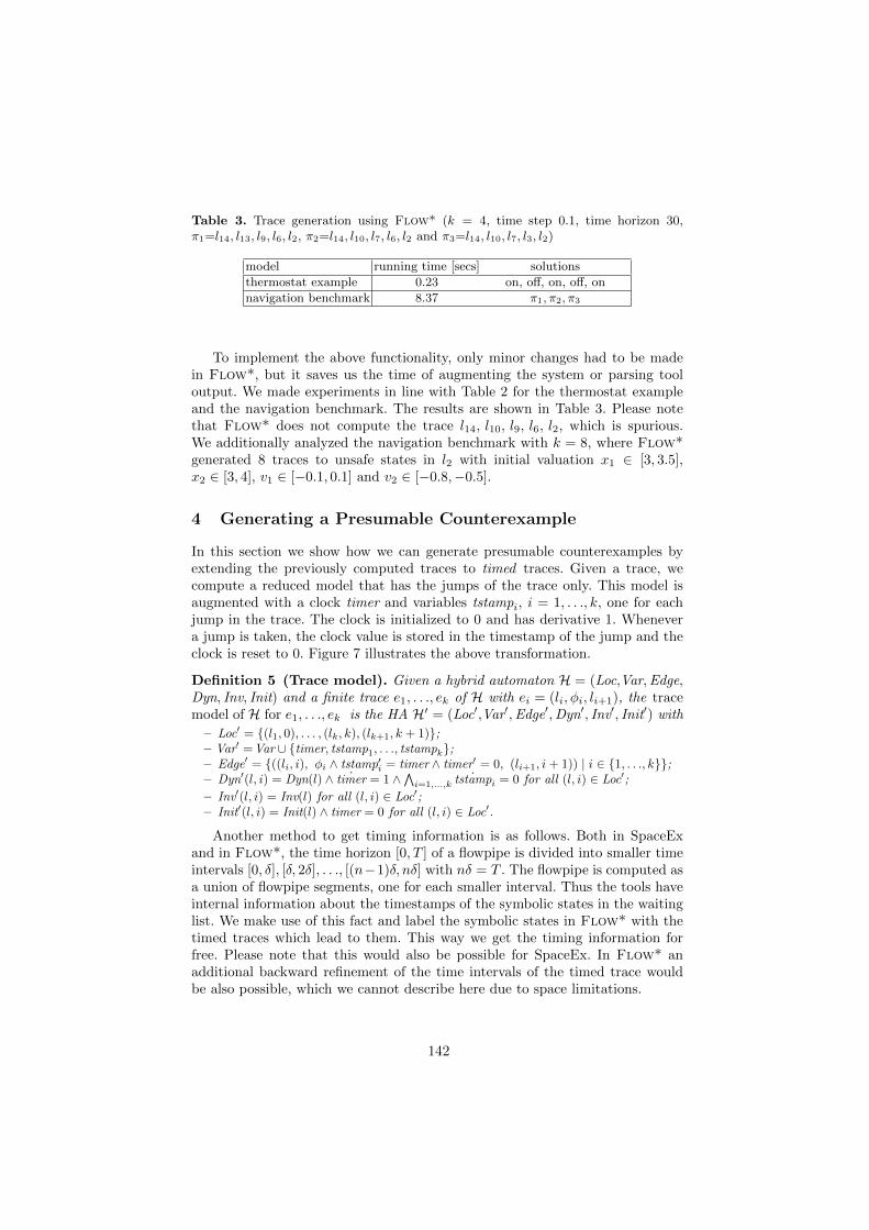
Table 3. Trace generation using Flow* (k = 4, time step 0.1, time horizon 30,π1=l14, l13, l9, l6, l2, π2=l14, l10, l7, l6, l2 and π3=l14, l10, l7, l3, l2)

model running time [secs] solutions

thermostat example 0.23 on, off, on, off, on

navigation benchmark 8.37 π1, π2, π3

To implement the above functionality, only minor changes had to be madein Flow*, but it saves us the time of augmenting the system or parsing tooloutput. We made experiments in line with Table 2 for the thermostat exampleand the navigation benchmark. The results are shown in Table 3. Please notethat Flow* does not compute the trace l14, l10, l9, l6, l2, which is spurious.We additionally analyzed the navigation benchmark with k = 8, where Flow*generated 8 traces to unsafe states in l2 with initial valuation x1 ∈ [3, 3.5],x2 ∈ [3, 4], v1 ∈ [−0.1, 0.1] and v2 ∈ [−0.8,−0.5].

4 Generating a Presumable Counterexample

In this section we show how we can generate presumable counterexamples byextending the previously computed traces to timed traces. Given a trace, wecompute a reduced model that has the jumps of the trace only. This model isaugmented with a clock timer and variables tstampi, i = 1, . . ., k, one for eachjump in the trace. The clock is initialized to 0 and has derivative 1. Whenevera jump is taken, the clock value is stored in the timestamp of the jump and theclock is reset to 0. Figure 7 illustrates the above transformation.

Definition 5 (Trace model). Given a hybrid automaton H = (Loc,Var,Edge,Dyn, Inv, Init) and a finite trace e1, . . ., ek of H with ei = (li, φi, li+1), the tracemodel of H for e1, . . ., ek is the HA H′ = (Loc′,Var′,Edge′,Dyn′, Inv′, Init′) with

– Loc′ = {(l1, 0), . . . , (lk, k), (lk+1, k + 1)};– Var′ =Var ∪ {timer, tstamp1, . . ., tstampk};– Edge′ = {((li, i), φi ∧ tstamp′i = timer ∧ timer′ = 0, (li+1, i+ 1)) | i ∈ {1, . . ., k}};– Dyn′(l, i) = Dyn(l) ∧ ˙timer = 1 ∧∧i=1,...,k

˙tstampi = 0 for all (l, i) ∈ Loc′;– Inv′(l, i) = Inv(l) for all (l, i) ∈ Loc′;– Init′(l, i) = Init(l) ∧ timer = 0 for all (l, i) ∈ Loc′.

Another method to get timing information is as follows. Both in SpaceExand in Flow*, the time horizon [0, T ] of a flowpipe is divided into smaller timeintervals [0, δ], [δ, 2δ], . . ., [(n−1)δ, nδ] with nδ = T . The flowpipe is computed asa union of flowpipe segments, one for each smaller interval. Thus the tools haveinternal information about the timestamps of the symbolic states in the waitinglist. We make use of this fact and label the symbolic states in Flow* with thetimed traces which lead to them. This way we get the timing information forfree. Please note that this would also be possible for SpaceEx. In Flow* anadditional backward refinement of the time intervals of the timed trace wouldbe also possible, which we cannot describe here due to space limitations.

142

on0

t ≤ 22

t = 1 ∧ ˙timer = 1∧∧i∈{1,...,3} ˙tstampi = 0

off1

t ≥ 18

t = 1 ∧ ˙timer = 1∧∧i∈{1,...,3} ˙tstampi = 0

on2

t ≤ 22

t = 1 ∧ ˙timer = 1∧∧i∈{1,...,3} ˙tstampi = 0

off3

t ≥ 18

t = 1 ∧ ˙timer = 1∧∧i∈{1,...,n} ˙tstampi = 0

t ≥ 21 ∧ tstamp′1 = timer

∧timer′ = 0

t ≤ 19 ∧ tstamp′2

= timer

∧timer′ = 0

t ≥ 21 ∧ tstamp′3 = timer

∧timer′ = 0

t = 20 ∧ timer = 0∧∧

i∈{1,...,n} tstampi = 0

Fig. 7. Trace model of the thermostat example for k = 3

Table 4. Comparison of the timed traces for the navigation benchmark computed bySpaceEx and Flow* (k = 4, time step 0.1, time horizon 30, traces from Table 2 and3)

Initial states: l14, x1 ∈ [3.0, 3.8], x2 ∈ [3.0, 4.0], v1 ∈ [−0.1, 0.1], v2 ∈ [−0.8,−0.5]

SpaceEx result in 6.46s:π1 : l14, [0.0, 0.6], l13, [0.0,1.4], l9, [1.5,1.8], l6, [2.3, 2.5], l2π2 : l14, [0.0, 1.9], l10, [1.5, 1.9], l7, [0.2, 2.5], l6, [0.0, 2.4], l2π3 : l14, [0.0, 1.9], l10, [1.5, 1.9], l7, [2.3, 2.5], l3, [0.0, 1.0], l2π4 : l14, [0.0, 1.9], l10, [0.0, 0.6], l9, [0.9, 1.4], l6, [0.0, 0.0], l2Flow* result in 8.37s:π1 : l14, [0.000,0.566], l13, [0.000, 1.420], l9, [1.531, 1.880], l6, [2.421,2.422], l2π2 : l14, [0.000,1.854], l10, [1.534,1.836], l7, [0.310,2.371], l6, [0.000,2.385], l2π3 : l14, [0.000,1.854], l10, [1.534,1.836], l7, [2.415,2.416], l3, [0.000,0.912], l2

Table 4 shows some experimental results for the navigation benchmark. Wecompute timed extensions of the previously computed counterexample traces tobuild presumable counterexamples. The running times include for Flow* a com-plete reachability analysis up to jump depth 4, and for SpaceEx the generation ofthe traces with Approach II and extracting timing information by building andanalyzing the trace models. Both tools have their advantages: SpaceEx computesthe results faster, Flow* gives sometimes better refinements.

5 Simulation

To gain counterexamples, we identifying some suitable candidate initial statesfrom the initial state set and refine the timed trace by restricting the timinginformations to the chosen state. Then we apply simulation heuristically to findconcrete counterexamples contained in the refined timed traces.

The task of finding initial state candidates for simulation is non-trivial, sincethe timed traces over-approximate counterexamples, such that not all initialstates lead to unsafe states within the given time bounds. W.l.o.g. we assumethat the initial set is given as a hyperrectangle (otherwise we over-approximatethe initial set by a hyperrectangle and use in the following the conjunction of

143

the hyperrectangle with the initial set). We obtain single initial state candidatesby applying a binary search on the initial set combined with an analysis runto check whether the unsafe states are still reachable. As long as unsafe statescan be reached from a hyperrectangle and in at least one dimension its width islarger than a specified parameter ε, the corner points of the hyperrectangle areadded to the set of initial state candidates and the interval is splitted (in onedimension in the middle). The binary search stops if either the specified numberof candidates are computed or if all hyperrectangles reached the minimal width.

The user can choose between a depth- (DFS) and a breadth-first search (BFS)to generate initial state candidates. DFS computes closely lying points fast, BFSsearches for widely spread points at a higher computation time.

For the trace l14, l10, l7, l6, l2 of the navigation benchmark, our implemen-tation needs 19ms to create the trace model. For the DFS SpaceEx has to berun 42 times until 10 points from the initial set from which the unsafe state l2is reachable are computed. The corresponding computation time is 7.14s. TheBFS finds the first 10 points within 29.90s and 133 SpaceEx calls.

Given a set of initial state candidates, we use adaptive step-size numeri-cal simulation to validate timed traces as counterexamples. Please note that forlinear differential equations the initial value problem is solvable, i.e., we can com-pute for each state the (unique) state reachable from it in time δ; however, sinceexponential function values must be determined, the computation is still notexact. The simulation starts at the initial state candidates, whereas the visitedmodes and the flow durations are restricted to the specifications in the timedtrace. Non-determinism (at which time point a jump is taken) is handled byselecting a homogeneously distributed set of time points from the given allowedtime interval and branching the simulation for each selected time point. How-ever, these time points are dynamically adapted in certain cases, for examplewhen otherwise edge guards or invariants would not be satisfied. We also de-veloped some optimizations, which we cannot describe here in detail, to reducethe number of simulations needed. The basic idea is to stop simulation branchesthat cannot lead to unsafe states as early as possible.

Table 5 shows the simulation results for some timed traces, each with a singleinitial state. Note that we find counterexamples (i.e., we reach the maximal jumpdepth) only in the two middle cases. We additionally run SpaceEx analyses withthe given initial point for the first trace and could not reach the bad state witha time step of 0.001, i.e., the first timed trace is spurious. The last trace was notcomputed by Flow* and is therefore spurious.

6 Conclusion and Future Work

In this paper we described an approach to find presumable counterexamples forhybrid automata based on existing reachability tools. Next we plan to improveour method by (1) a backward refinement of the time intervals on timed paths,(2) a rigorous simulation technique for hybrid automata, (3) giving a betterheuristics to select the initial points for simulation and (4) use several tools

144

Table 5. Simulation results for the navigation benchmark with ε-enlargingπ1 = l14, [0.0, 0.2], l13, [0.0, 0.4], l9, [1.5, 1.6], l6, [2.4, 2.5], l2

with initial state (3.0084472656250005, 3.21875,−0.1,−0.8)π2 = l14, [1.834, 1.835], l10, [1.779, 1.78], l7, [1.934, 1.936], l6, [0.511, 0.514], l2

with initial state (3.2, 4.0, 0.1,−0.5)π3 = l14, [0.000, 0.001], l10, [1.569, 1.570], l7, [2.429, 2.431], l3, [0.514, 0.517], l2

with initial state (3.8, 3.0,−0.1,−0.8)π4 = l14, [0.0, 0.1], l10, [0.0, 0.5], l9, [1.0, 1.3], l6, [2.3, 2.5], l2

with initial state (3.0125, 3.0,−0.1,−0.8)

timed trace step size ε reached jump depth #simulated paths unsafe time [secs]

π1 0.0005 0.0005 2 128 · 108 0 20.910.05 0.5 3 128 0 04.26

π2 0.0005 0.5 4 964 > 50 14.82

π3 0.0005 0.05 4 96 > 50 14.440.0005 0.0005 4 96 50 10.51

π4 0.0005 0.0005 2 480 · 108 0 15.460.05 0.05 3 480 0 07.88

and take the best results to minimize the overestimation in a presumable coun-terexample. Preliminary results suggest that the function calculus of the toolAriadne can be used to validate counterexamples.

References

1. Alur, R., Courcoubetis, C., Halbwachs, N., Henzinger, T.A., Ho, P., Nicollin, X.,Olivero, A., Sifakis, J., Yovine, S.: The algorithmic analysis of hybrid systems.Theor. Comput. Sci. 138 (1995) 3–34

2. Frehse, G., Le Guernic, C., Donze, A., Lebeltel, R.R.O., Ripado, R., Girard, A.,Dang, T., Maler, O.: SpaceEx: Scalable verification of hybrid systems. In: Proc.of CAV’11. Volume 6806 of LNCS., Springer (2011) 379–395

3. Chen, X., Abraham, E., Sankaranarayanan, S.: Flow*: An analyzer for non-linearhybrid systems. In: Proc. of CAV’13. Volume 8044 of LNCS., Springer (2013)258–263

4. Stursberg, O., Krogh, B.H.: Efficient representation and computation of reachablesets for hybrid systems. In: Proc. of HSCC’03. Volume 2623 of LNCS., Springer(2003) 482–497

5. Chutinan, A., Krogh, B.H.: Computing polyhedral approximations to flow pipes fordynamic systems. In: Proc. of CDC’98 (volume 2), IEEE Press (1998) 2089–2094

6. Henzinger, T.A., Ho, P., Wong-Toi, H.: HyTech: A model checker for hybrid sys-tems. Software Tools for Technology Transfer 1 (1997) 110–122

7. Frehse, G.: PHAVer: Algorithmic verification of hybrid systems past HyTech. In:Proc. of HSCC’05. Volume 3414 of LNCS., Springer (2005) 258–273

8. Kvasnica, M., Grieder, P., Baotic, M.: Multi-parametric toolbox (MPT) (2004)http://control.ee.ethz.ch/∼mpt/.

9. Chen, X., Abraham, E.: Choice of directions for the approximation of reachablesets for hybrid systems. In: Proc. of EUROCAST’11. Volume 6927 of LNCS.,Springer (2011) 535–542

145

10. Kuhn, W.: Zonotope dynamics in numerical quality control. In: MathematicalVisualization: Algorithms, Applications and Numerics. Springer (1998) 125–134

11. Girard, A.: Reachability of uncertain linear systems using zonotopes. In: Proc. ofHSCC’05. Volume 3414 of LNCS., Springer (2005) 291–305

12. Bournez, O., Maler, O., Pnueli, A.: Orthogonal polyhedra: Representation andcomputation. In: Proc. of HSCC’99. Volume 1569 of LNCS., Springer (1999) 46–60

13. Kurzhanski, A.B., Varaiya, P.: On ellipsoidal techniques for reachability analysis.Optimization Methods and Software 17 (2000) 177–237

14. Le Guernic, C.: Reachability Analysis of Hybrid Systems with Linear ContinuousDynamics. PhD thesis, Universite Joseph Fourier (2009)

15. Le Guernic, C., Girard, A.: Reachability analysis of hybrid systems using supportfunctions. In: Proc. of CAV’09. Volume 5643 of LNCS., Springer (2009) 540–554

16. Chen, X., Abraham, E., Sankaranarayanan, S.: Taylor model flowpipe constructionfor non-linear hybrid systems. In: Proc. of RTSS’12, IEEE Computer Society (2012)183–192

17. Collins, P., Bresolin, D., Geretti, L., Villa, T.: Computing the evolution of hy-brid systems using rigorous function calculus. In: Proc. of ADHS’12, IFAC-PapersOnLine (2012)

18. Mitchell, I., Tomlin, C.: Level set methods for computation in hybrid systems. In:Proc. of HSCC’00. Volume 1790 of LNCS., Springer (2000) 310–323

19. Asarin, E., Dang, T., Maler, O.: The d/dt tool for verification of hybrid systems.In: Proc. of CAV’02. Volume 2404 of LNCS., Springer (2002) 365–370

20. Girard, A., Pappas, G.J.: Approximation metrics for discrete and continuous sys-tems. IEEE Transactions on Automatic Control 52 (2007) 782–798

21. Kurzhanskiy, A., Varaiya, P.: Ellipsoidal toolbox. Technical report, EECS, UCBerkeley (2006)

22. Balluchi, A., Casagrande, A., Collins, P., Ferrari, A., Villa, T., Sangiovanni-Vincentelli, A.L.: Ariadne: A framework for reachability analysis of hybrid au-tomata. In: Proc. of MTNS’06. (2006)

23. Prabhakar, P., Duggirala, P.S., Mitra, S., Viswanathan, M.: Hybrid automata-based CEGAR for rectangular hybrid systems. In: Proc. of VMCAI’13. Volume7737 of LNCS., Springer (2013) 48–67

24. Duggirala, P.S., Mitra, S.: Abstraction refinement for stability. In: Proc. of IC-CPS’11, IEEE (2011) 22–31

25. Fehnker, A., Ivancic, F.: Benchmarks for hybrid systems verification. In: Proc. ofHSCC’04. Volume 2993 of LNCS., Springer (2004) 326–341

146

Compositional Nonblocking Verificationwith Always Enabled Events and Selfloop-only Events

Colin Pilbrow Robi Malik

Department of Computer Science, University of Waikato, Hamilton, New Zealandcolinpilbrow@gmail.com robi@waikato.ac.nz

Abstract. This paper proposes to improve compositional nonblocking verifica-tion through the use of always enabled and selfloop-only events. Compositionalverification involves abstraction to simplify parts of a system during verification.Normally, this abstraction is based on the set of events not used in the remain-der of the system, i.e., in the part of the system not being simplified. Here, it isproposed to exploit more knowledge about the system and abstract events eventhough they are used in the remainder of the system. Abstraction rules from previ-ous work are generalised, and experimental results demonstrate the applicabilityof the resulting algorithm to verify several industrial-scale discrete eventsystemmodels, while achieving better state-space reduction than before.

1 Introduction

The nonblocking propertyis a weak liveness property commonly used insupervisorycontrol theoryof discrete event systems to express the absence of livelocks or dead-locks [6, 24]. This is a crucial property of safety-criticalcontrol systems, and with theincreasing size and complexity of these systems, there is anincreasing need to verifythe nonblocking property automatically. The standard method to check whether a sys-tem is nonblocking involves the explicit composition of allthe automata involved, andis limited by the well-knownstate-space explosionproblem.Symbolic model checkinghas been used successfully to reduce the amount of memory required by representingthe state space symbolically rather than enumerating it explicitly [2].

Compositional verification[11, 29] is an effective alternative that can be used in-dependently of or in combination with symbolic methods. Compositional verificationworks by simplifying individual automata of a large synchronous composition, gradu-ally reducing the state space of the system and allowing muchlarger systems to be ver-ified in the end. When applied to the nonblocking property, compositional verificationrequires very specific abstraction methods [10,19]. A suitable theory is laid out in [20],where it is argued that abstractions used in nonblocking verification should preservea process-algebraic equivalence calledconflict equivalence. Various abstraction rulespreserving conflict equivalence have been proposed and implemented [10,19,22,27].

Conflict equivalence is the most general process equivalence for use in composi-tional nonblocking verification [20]. If a part of a system isreplaced by a conflict equiv-alent abstraction, the nonblocking property is guaranteedto be preserved independentlyof the other components of the system. While this is easy to understand and implement,

147

more simplification is possible by considering the other system components. This pa-per proposes simplification rules that take into account that certain events are alwaysenabled or only selfloops in the rest of the system, and showshow this additional infor-mation can achieve further state-space reduction.

In the following, Section 2 introduces the background of nondeterministic automata,the nonblocking property, and conflict equivalence. Next, Section 3 describes compo-sitional verification and always enabled and selfloop-onlyevents. Section 4 presentssimplification rules that exploit such events, and Section 5shows how these events arefound algorithmically. Afterwards, Section 6 presents theexperimental results, and Sec-tion 7 adds concluding remarks. Further details and formal proofs of technical resultswill be available in [23].

2 Preliminaries

2.1 Events and Languages

Event sequences and languages are a simple means to describediscrete system be-haviours [6, 24]. Their basic building blocks areevents, which are taken from a finitealphabetA. In addition, two special events are also used, thesilent eventτ and thetermination eventω. These are never included in an alphabetA unless mentioned ex-plicitly using notation such asAτ = A∪{τ}, Aω = A∪{ω}, andAτ ,ω = A∪{τ,ω}.

A∗ denotes the set of all finitetracesof the form σ1σ2 · · ·σn of events fromA,including theempty traceε. Theconcatenationof two tracess, t ∈ A∗ is written asst.A subsetL ⊆ A∗ is called alanguage. The natural projection P: A∗

τ ,ω → A∗ω is the

operation that deletes all silent (τ) events from traces.

2.2 Nondeterministic Automata

System behaviours are modelled using finite automata. Typically, system models aredeterministic, but abstraction may result in nondeterminism.

Definition 1. A (nondeterministic)finite automatonis a tupleG= 〈A ,Q,→,Q◦〉whereA is a finite set ofevents, Q is a finite set ofstates, → ⊆ Q×Aτ ,ω ×Q is thestatetransition relation, andQ◦ ⊆ Q is the set ofinitial states.

The transition relation is written in infix notationxσ→ y, and is extended to traces

s∈ A∗τ ,ω in the standard way. For state setsX,Y ⊆ Q, the notationX

s→Y meansxs→ y

for somex ∈ X andy ∈ Y, andXs→ y meansx

s→ y for somex ∈ X. Also, Xs→ for a

state or state setX denotes the existence of a statey∈ Q such thatXs→ y.

The termination eventω /∈ A denotes completion of a task and does not appearanywhere else but to mark such completions. It is required that states reached byωdo not have any outgoing transitions, i.e., ifx

ω→ y then there does not existσ ∈ Aτ ,ω

such thatyσ→. This ensures that the termination event, if it occurs, is always the final

event of any trace. The traditional set ofterminalstates isQω = {x∈ Q | xω→} in this

notation. For graphical simplicity, states inQω are shown shaded in the figures of thispaper instead of explicitly showingω-transitions.

148

To support silent events, another transition relation⇒⊆ Q×A∗ω ×Q is introduced,

wherexs⇒ y denotes the existence of a tracet ∈A∗

τ ,ω such thatP(t) = sandxt→ y. That

is, xs→ y denotes a path withexactlythe events ins, while x

s⇒ y denotes a path withan arbitrary number ofτ events shuffled with the events ofs. Notations such asX

s⇒Yandx

s⇒ are defined analogously to→.

Definition 2. Let G = 〈AG,QG,→G,Q◦G〉 and H = 〈AH ,QH ,→H ,Q◦

H〉 be two auto-mata. Thesynchronous compositionof G andH is

G‖H = 〈AG∪AH ,QG×QH ,→,Q◦H ×Q◦

H〉 , (1)

where

– (xG,xH)σ→ (yG,yH) if σ ∈ (AG∩AH)∪{ω}, xG

σ→G yG, andxHσ→H yH ;

– (xG,xH)σ→ (yG,xH) if σ ∈ (AG\AH)∪{τ} andxG

σ→G yG;– (xG,xH)

σ→ (xG,yH) if σ ∈ (AH \AG)∪{τ} andxHσ→H yH .

Automata are synchronised using lock-step synchronisation [13]. Shared events (in-cludingω) must be executed by all automata synchronously, while other events (includ-ing τ) are executed independently.

2.3 The Nonblocking Property

The key liveness property in supervisory control theory is thenonblockingproperty. Anautomaton is nonblocking if, from every reachable state, a terminal state can be reached;otherwise it isblocking. When more than one automaton is involved, it also is commonto use the termsnonconflictingandconflicting.

Definition 3. [20] An automatonG= 〈A ,Q,→,Q◦〉 is nonblockingif, for every state

x∈ Q and every traces∈ A∗ such thatQ◦ s⇒ x, there exists a tracet ∈ A∗ such thatxtω⇒.

Two automataG andH arenonconflictingif G‖H is nonblocking.

To reason about conflicts in a compositional way, the notion of conflict equivalenceis developed in [20]. According to process-algebraic testing theory, two automata areconsidered as equivalent if they both respond in the same wayto tests [7]. Forcon-flict equivalence, a test is an arbitrary automaton, and theresponseis the observationwhether the test composed with the automaton in question is nonblocking or not.

Definition 4. [20] Two automataG andH areconflict equivalent, written G≃conf H,if, for any automatonT, G‖T is nonblocking if and only ifH ‖T is nonblocking.

3 Compositional Verification

When verifying whether a composed system of automata

G1‖G2‖ · · · ‖Gn , (2)

149

is nonblocking, compositional methods [10, 19] avoid building the full synchronouscomposition immediately. Instead, individual automataGi are simplified and replacedby smaller conflict equivalent automataHi ≃conf Gi . If no simplification is possible, asubsystem of automata(G j) j∈J is selected and replaced by its synchronous composi-tion, which then may be simplified.

The soundness of this approach is justified by thecongruenceproperties [20] ofconflict equivalence. For example, ifG1 in (2) is replaced byH1 ≃conf G1, then byconsideringT = G2 ‖ · · · ‖Gn in Def. 4, it follows that the abstracted systemH1 ‖T =H1‖G2‖ · · · ‖Gn is nonblocking if and only if the original system (2) is.

Previous approaches for compositional nonblocking verification [10, 19] are basedon local events. A componentG1 in a system such as (2) typically contains some eventsthat appear only inG1 and not in the remainderT = G2 ‖ · · · ‖Gn of the system. Theseevents are called local and are abstracted using hiding, i.e., they are replaced by thesilent eventτ. Conflict equivalence usesτ as a placeholder for events not used else-where, and in this setting is the coarsest conflict-preserving abstraction [20].

Yet, in practice, the remainderT =G2‖· · ·‖Gn is known. This paper proposes waysto use additional information aboutT to inform the simplification ofG1 and producebetter abstractions. In addition to using theτ events, it can be examined how otherevents are used byT. There are two kinds of events that are easy to detect:alwaysenabledevents andself loop-onlyevents.

Definition 5. Let G= 〈A ,Q,→,Q◦〉 be an automaton. An eventσ ∈ A is always en-

abledin G, if for every statex∈ Q it holds thatxσ⇒.

An event is always enabled in an automaton if it can be executed from every state—possibly after some silent events. If during compositionalverification, an event is foundto be always enabled in every automaton except the one being simplified, this event hassimilar properties to a silent event. Several abstraction methods that exploit silent eventsto simplify automata can be generalised to exploit always enabled events also.

Definition 6. Let G= 〈A ,Q,→,Q◦〉 be an automaton. An eventσ ∈ A is selfloop-only

in G, if for every transitionxσ→ y it holds thatx= y.

Selfloopsare transitions that have the same start and end states. An event is selfloop-only if it only appears on selfloop transitions. As the presence of selfloops does notaffect the nonblocking property, the knowledge that an event is selfloop-only can helpto simplify the system beyond standard conflict equivalence. In the following definition,conflict equivalence is generalised by considering setsE andSof events that are alwaysenabled or selfloop-only in the rest of the system, i.e., in the testT.

Definition 7. Let G andH be two automata, and letE andS be two sets of events.GandH areconflict equivalentwith respect toE andS, written G ≃E,S H, if for everyautomatonT such thatE is a set of always enabled events inT andS is a set of selfloop-only events inT, it holds thatG‖T is nonblocking if and only ifH ‖T is nonblocking.

Clearly, standard conflict equivalence implies conflict equivalence with respect toE andS, as the latter considers fewer testsT. Yet, both equivalences have the sameuseful properties for compositional nonblocking verification. The following results areimmediate from the definition.

150

G

PSfrag

0 1

2 3

τ

α

α β

βη

H

2 3

01

α

α

β

βη

T 0

1

αβη

G‖T (0,0)(1,0)

(1,2)

τ

α

H ‖T (0,0)

(1,2)

α

Fig. 1.Two automataG andH such thatG≃{η}, /0 H but notG≃conf H.

Proposition 1. Let G andH be two automata.

(i) G≃conf H if and only if G≃ /0, /0 H.(ii) If E ⊆ E′ andS⊆ S′ thenG≃E,S H impliesG≃E′,S′ H.

Proposition 2. LetG1, . . . ,Gn andH1 be automata such thatG1 ≃E,S H1, whereE andSare sets of events that respectively are always enabled and selfloop-only forG2‖· · ·‖Gn.ThenG1‖ · · · ‖Gn is nonblocking if and only ifH1‖G2‖ · · · ‖Gn is nonblocking.

Prop. 1 confirms that conflict equivalence with respect toE andS is coarser thanstandard conflict equivalence and considers more automata as equivalent. Thus, themodified equivalence has the potential to achieve better abstraction. At the same time,Prop. 2 shows that the modified equivalence can be used in the same way as standardconflict equivalence to replace automata in compositional verification, provided thatsuitable event setsE andScan be determined.

Example 1. AutomataG andH in Fig. 1 arenot conflict equivalent as demonstratedby the test automatonT. On the one hand,G‖T is blocking because the state(1,0)is reachable byτ from the initial state(0,0), and(1,0) is a deadlock state, becauseGdisables eventα in state 1 andT disables eventsβ andη in state 0. On the other hand,H ‖T is nonblocking.

Note thatη is not always enabled inT since 0η⇒T does not hold. In composition

with a testT that hasη always enabled,G will be able to continue from state 1, andHwill be able to continue from state 01. It follows from Prop. 4below thatG≃{η}, /0 H.

4 Simplification Rules

To exploit conflict equivalence in compositional verification, it is necessary to algorith-mically compute a conflict equivalent abstraction of a givenautomaton. Several abstrac-tion rules are known for standard conflict equivalence [10,19]. This section generalisessome of these and proposes four computationally feasible rules to simplify automataunder the assumption of always enabled and selfloop-only events. Before that, Subsec-tion 4.1 introduces general terminology to describe all abstractions.

4.1 Automaton Abstraction

A common method to simplify an automaton is to construct itsquotientmodulo anequivalence relation. The following definitions are standard.

151

An equivalence relationis a binary relation that is reflexive, symmetric and transi-tive. Given an equivalence relation∼ on a setQ, theequivalence classof x ∈ Q withrespect to∼, denoted[x], is defined as[x] = {x′ ∈ Q | x′ ∼ x}. An equivalence relationon a setQ partitionsQ into the setQ/∼= { [x] | x∈ Q} of its equivalence classes.

Definition 8. Let G= 〈A ,Q,→,Q◦〉 be an automaton, and let∼⊆ Q×Q be an equiv-alence relation. Thequotient automaton G/∼ of G with respect to∼ is G/∼ = 〈A,

Q/∼ ,→/∼ ,Q◦〉, whereQ◦ = { [x◦] | x◦ ∈ Q◦ } and→/∼= {([x],σ , [y]) | xσ→ y}.

When constructing a quotient automaton, classes of equivalent states in the originalautomaton are combined ormergedinto a single state. A common equivalence relationto construct quotient automata isobservation equivalenceor weak bisimulation[21].

Definition 9. [21] Let G= 〈A ,Q,→,Q◦〉 be an automaton. A relation≈ ⊆ Q×Q isanobservation equivalencerelation onG if, for all statesx1,x2 ∈ Q such thatx1 ≈ x2

and all tracess∈ A∗ω the following conditions hold:

(i) if x1s⇒ y1 for somey1 ∈ Q, then there existsy2 ∈ Q such thaty1 ≈ y2 andx2

s⇒ y2;(ii) if x2

s⇒ y2 for somey2 ∈ Q, then there existsy1 ∈ Q such thaty1 ≈ y2 andx1s⇒ y1.

Two states are observation equivalent if they have got exactly the same sequencesof enabled events, leading to equivalent successor states.Observation equivalence isa well-known equivalence with efficient algorithms that preserves all temporal logicproperties [5]. In particular, an observation equivalent abstraction is conflict equivalentto the original automaton.

Proposition 3. [19] Let G be an automaton, and let≈ be an observation equivalencerelation onG. ThenG≃conf G/≈.

A special case of observation equivalence-based abstraction is τ-loop removal. Iftwo states are mutually connected by sequences ofτ-transitions, it follows from Def. 9that these states are observation equivalent, so by Prop. 3 they can be merged preservingconflict equivalence. This simple abstraction results in aτ-loop freeautomaton, i.e., anautomaton that does not contain any proper cycles ofτ-transitions.

Definition 10. Let G = 〈A ,Q,→,Q◦〉 be an automaton.G is τ-loop free, if for every

pathxt→ x with t ∈ {τ}∗ it holds thatt = ε.

While τ-loop removal and observation equivalence are easy to compute and pro-duce good abstractions, there are conflict equivalent automata that are not observationequivalent. Several other relations are considered for conflict equivalence [10,19].

Definition 11. [10] Let G = 〈A ,Q,→,Q◦〉 be an automaton. Theincoming equiva-lencerelation∼inc ⊆ Q×Q is defined such thatx∼inc y if,

(i) Q◦ ε⇒ x if and only if Q◦ ε⇒ y;(ii) for all statesw∈ Q and all eventsσ ∈ A it holds thatw

σ⇒ x if and only if wσ⇒ y.

Two states are incoming equivalent if they have got the same incoming transitionsfrom the exactly same source states. (This is different fromreverse observation equiv-alence, which acceptsequivalentrather than identical states.) Incoming equivalencealone is not enough for conflict-preserving abstraction. Itis combined with other con-ditions in the following.

152

4.2 Enabled Continuation Rule

The Enabled Continuation Rule is a generalisation of the Silent Continuation Rule [10],which allows to merge incoming equivalent states in aτ-loop free automaton providedthey have both have an outgoingτ-transition. The reason for this is that, if a state hasan outgoingτ-transition, then the other outgoing transitions are “optional” [10] for atest that is to be nonblocking with this automaton. Only continuations from states with-out furtherτ-transitions must be present in the test. Using always enabled events, thecondition onτ-transitions can be relaxed: it also becomes possible to merge incomingequivalent states if they have outgoing always enabled transitions instead ofτ.

Rule 1 (Enabled Continuation Rule).In a τ-loop free automaton, two states that areincoming equivalent and both have an outgoingalways enabledor τ-transition are con-flict equivalent and can be merged.

Example 2. Consider automatonG in Fig. 1 with E = {η}. States 0 and 1 are both“initial” since they both can be reached silently from the initial state 0. This is enoughto satisfy∼inc in this case, since neither state is reachable by any event other thanτ.Moreover,G has noτ-loops, state 0 has an outgoingτ-transition, and state 1 has anoutgoing always enabled eventη . Thus, by the Enabled Continuation Rule, states 0and 1 inG are conflict equivalent and can be merged into state 01 as shown in H.

Note that states 0 and 1 are not observation equivalent because 0α→ 2 while state 1

has no outgoingα-transition. The Silent Continuation Rule [10] also is not applicablebecause state 1 has no outgoingτ-transition. Only with the additional information thatη is always enabled, it becomes possible to merge states 0 and 1.

Proposition 4. Let G= 〈A,Q,→G,Q◦〉 be aτ-loop free automaton, letE ⊆ A, and let∼⊆ Q×Q be an equivalence relation such that∼⊆∼inc, and for allx,y∈ Q such that

x∼ y it holds that eitherx= y or xη1⇒ andy

η2⇒ for some eventsη1,η2 ∈ E∪{τ}. ThenG≃E, /0 G/∼.

Prop. 4 confirms that the nonblocking property of the system is preserved under thegeneralised silent continuation rule, provided thatE is a set of always enabled eventsfor the remainder of the system.

4.3 Only Silent Incoming Rule

The Only Silent Incoming Rule [10] is a combination of observation equivalence andthe Silent Continuation Rule. Since the Silent Continuation Rule has been generalisedto use always enabled events, the Only Silent Incoming Rule can as well.

The original Only Silent Incoming Rule [10] makes it possible to remove a statewith only τ-transitions incoming and merge it into its predecessors, provided that theremoved state has got at least one outgoingτ-transition. Again, the requirement for anoutgoingτ-transition can be relaxed to allow an always enabled transition also.

Rule 2 (Only Silent Incoming Rule).If a τ-loop free automaton has a stateq with onlyτ-transitions entering it, and an always enabled orτ-transition outgoing from stateq,then all transitions outgoing fromq can can be copied to originate from the states withτ-transitions toq. Afterwards, theτ-transitions toq can be removed.

153

G 0 1

2 3τ

τα α

ββ

γ

η

G′ 0 1

2 3a

3b

τ

τ

αα

α

ββ

γη

η

H 0 1

2

αα α

ββ

γ

ηη

Fig. 2. Example of application of the Only Silent Incoming Rule.

G0 1

2 3τ

α α

β

η

H0 1

2 3

α

β H ′0

⊥α ,β

Fig. 3.Example of application of the Limited Certain Conflicts Rule.

Example 3. In Fig. 2 it holds thatG≃{η}, /0 H. State 3 inG has onlyτ-transitions in-coming and the always enabled eventη outgoing. This state can be removed in twosteps. First, state 3 is split into two observation equivalent states 3a and 3b in G′, andafterwards the Silent Continuation Rule is applied to mergethese states into their in-coming equivalent predecessors, resulting inH. Note that states 1, 2, and 3 are notobservation equivalent because of theβ - andγ-transitions from states 1 and 2.

Proposition 5. Let G= 〈A,Q,→G,Q◦〉 be aτ-loop free automaton, and letE ⊆ A. Let

q ∈ Q such thatqη→G for someη ∈ E∪{τ}, and for each transitionx

σ→G q it holdsthatσ = τ. Further, letH = 〈A,Q,→H ,Q◦〉 with

→H = {(x,σ ,y) | xσ→G y andy 6= q} ∪ {(x,σ ,y) | x

τ→G qσ→G y} . (3)

ThenG≃E, /0 H.

It is shown in [10] that the Only Silent Incoming Rule can be expressed as a com-bination of observation equivalence and the Silent Continuation Rule as suggested inExample 3. The same argument can be used to prove Prop. 5.

4.4 Limited Certain Conflicts Rule

If an automaton contains blocking states, i.e., states fromwhere no state with anω-transition can be reached, then a lot of simplification is possible. Once a blocking stateis reached, all further transitions are irrelevant. Therefore, all blocking states can bemerged into a single state, and all their outgoing transitions can be deleted [18].

In fact, this rule does not only apply to blocking states. Forexample, consider state 3in automatonG in Fig. 3. Despite the fact that 3

ω→, i.e., 3 is a terminal state, if state 3is ever reached, the composed system is necessarily blocking, as nothing can prevent itfrom executing the silent transition 3

τ→ 2 to the blocking state 2. State 3 is a state ofcertain conflicts, and such states can be treated like blocking states for the purpose ofabstraction.

154

It is possible to calculate all states of certain conflicts, but the algorithm to do thisis exponential in the number of states of the automaton to be simplified [18]. To reducethe complexity, the Limited Certain Conflicts Rule [10] approximates the set of certainconflicts. If a state has aτ-transition to a blocking state, then the source state alsois a state of certain conflicts. This can be extended to include always enabled events,because if an always enabled transition takes an automaton to a blocking state, thennothing can disable this transition and the composed systemis necessarily blocking.

Rule 3 (Limited Certain Conflicts Rule). If an automaton contains an always enabledor τ-transition to a blocking state, then the source state of this transition is a state ofcertain conflicts, and all its outgoing transitions can be deleted.

Example 4. Consider automatonG in Fig. 3 with E = {η}. States 1, 2, and 3 arestates of certain conflicts. State 2 is already blocking, andstates 1 and 3 have aτ- oran always enabledη-transition to the blocking state 2. All outgoing transitions fromthese states are removed, including theω-transitions from states 1 and 3. This results inautomatonH. Now state 3 is unreachable and can be removed, and states 1 and 2 can bemerged using observation equivalence to createH ′. It holds thatG≃{η}, /0 H ≃conf H ′.

Proposition 6. Let G = 〈A,Q,→G,Q◦〉 be an automaton andE ⊆ A, let q ∈ Q be a

blocking state, and letpη→ q for someη ∈ E∪{τ}. Furthermore, letH = 〈A,Q,→H ,

Q◦〉 where→H = {(x,σ ,y) ∈→ | x 6= p}. ThenG≃E, /0 H.

Prop. 6 confirms that a state with aτ- or always enabled transitions to some otherblocking state can also be made blocking, by deleting all outgoing transitions (includ-ing ω) from it. The Limited Certain Conflicts Rule should be applied repeatedly, as thedeletion of transitions may introduce new blocking states and thus new certain conflicts.

4.5 Selfloop Removal Rule

The final abstraction rule concerns selfloop-only events. To verify nonblocking, it isenough to check if every state in the final synchronous composition of all automata canreach a terminal state. Selfloops in the final synchronous composition have no effect onthe blocking nature of the system, since any path between twostates passes the samestates if all selfloops are removed from the path. So, the final synchronous compositionis nonblocking if and only if it is nonblocking with all selfloops removed.

Based on this observation, if an event is known to be selfloop-only in all automataexcept the one being simplified, then selfloops with that event can be added or removedfreely to the automaton being simplified.

Rule 4 (Selfloop Removal Rule).If an eventλ is selfloop-only in all other automata,

then selfloop transitionsqλ→ q can be added to or removed from any stateq.

This rule can be used to remove selfloops and save memory, sometimes reducingthe amount of shared events or allowing other rules to be used. If an event only appearson selfloops in all automata, then it can be removed entirely. Furthermore, the additionof selfloops to certain states may also be beneficial.

155

G1 0

12 β

β

λ

λ

G2 0

12

β

β

λ

G3 0

12 β

β

λ

λ

G4 01

2

βλ G5 01

2

β

Fig. 4. Example of the removal and addition of selfloops.

Example 5. Fig. 4 shows a sequence of conflict-preserving changes to an automatoncontaining the selfloop-only eventλ . First, theλ -selfloop inG1 is removed to createG2.In G2, states 0 and 1 are close to observation equivalent, as they both have aβ -transitionto state 2; however 0 has aλ -transition to 1 and 1 does not. Yet, it is possible to add aλ -selfloop to state 1 and createG3. Now states 0 and 1 are observation equivalent andcan be merged to createG4. Finally, theλ -selfloop inG4 is removed to createG5.

Proposition 7. Let G = 〈A,Q,→G,Q◦〉 and H = 〈A,Q,→H ,Q◦〉 be automata with→H =→G∪{(q,λ ,q)} for someλ ∈ A. ThenG≃ /0,{λ} H.

Prop. 7 shows that the addition of a single selfloop preserves conflict equivalence.it can be applied in reverse to remove selfloops, and it can beapplied repeatedly to addor remove several selfloops in an automaton or in the entire system.

The implementation in Section 6 uses selfloop removal whenever applicable todelete as many selfloops as possible. In addition, observation equivalence has beenmodified to assume the presence of selfloops for all selfloop-only events in all states,so as to achieve the best possible state-space reduction.

5 Finding Always Enabled and Selfloop-only Events

While the simplification rules in Section 4 are straightforward extensions of knownrules for standard conflict equivalence [10], their application requires the knowledgeabout always enabled and selfloop-only events. Assume the system (2) encounteredduring compositional verification is

G1‖G2‖ · · · ‖Gn , (4)

and automatonG1 is to be simplified. Then it is necessary to know always enabledand selfloop-only events inT = G2 ‖ · · · ‖Gn. For each component automatonGi , suchevents are easy to detect based on Def. 5 and 6. It also is a direct consequence of thedefinitions that these properties carry over to the synchronous product.

Proposition 8. Let G1 andG2 be two automata. If an eventσ is always enabled (orselfloop-only) inG1 andG2, thenσ is always enabled (or selfloop-only) inG1‖G2.

Given Prop. 8, an event can be considered as always enabled orselfloop-only ifit has this property for every automaton in (4) except the automaton being simplified.When checking the individual automata, selfloop-only events are easily found by check-ing whether an event in question only appears on selfloop transitions. For always en-abled events, it is checked whether the event in question is enabled in every state, butadditional considerations can help to find more always enabled events.

156

G0 1

⊥τα

η G′

0 1

⊥τα

η

η

Fig. 5.Finding an always enabled event.

Example 6. Consider automatonG in Fig. 5. It clearly holds that 0η→, and 1

τ→ 0η→

and thus 1η⇒. Althoughη is not enabled in state⊥, this state is a blocking state and the

set of enabled events for blocking states is irrelevant—it isknown [18] thatG is conflictequivalent toG′. Thenη can be considered as always enabled inG′ and thus also inG.

By definition, an always enabled eventη must be possible in every state of the envi-ronmentT, except for blocking states according to Example 6. However, this conditionis stronger than necessary, asη typically is not always possible in the automatonGbeing simplified. This observation leads toconditionallyalways enabled events.

Definition 12. Let G= 〈A,QG,→G,Q◦G〉 andT = 〈A,QT ,→T ,Q◦

T〉 be two automata.An eventσ ∈ A is conditionally always enabledfor G in T, if for all s∈ A∗ such thatQ◦

Gsσ⇒G and all statesxT ∈ QT such thatQ◦

Ts⇒T xT , it holds thatxT

σ⇒T .

An event is conditionally always enabled if the environmentT enables it in all stateswhere it is possible in the automatonG to be simplified. The following Prop. 9 showsthat the result of compositional nonblocking verification is also preserved with eventsthat are only conditionally always enabled.

Proposition 9. Let G, H, andT be automata, and letE andS be event sets such thatG ≃E,S H, andE is a set of conditionally always enabled events forG in T, andS isa set of selfloop-only events forT. ThenG‖T is nonblocking if and only ifH ‖T isnonblocking.

Conditionally always enabled events can be used like general always enabled events,but they are more difficult to find. To check the condition of Def. 12, it is necessary toexplore the state space ofG‖T, which has the same complexity as a nonblocking check.Yet, the condition is similar tocontrollability [6], which can often be verified quickly byanincremental controllability check[4]. The incremental algorithm gradually composessome of the automata of the system (4) until it can be ascertained whether or not a givenevent is conditionally always enabled. In many cases, it gives a positive or negativeanswer after composing only a few automata.

By running the incremental controllability check for a short time, some condition-ally always enabled events can be found, while for others thestatus remains inconclu-sive. Fortunately, it is not necessary to find all always enabled events. If the status of anevent is not known, it can be assumed that this event isnotalways enabled. The result ofnonblocking verification will still be correct, although itmay not use the best possibleabstractions. It is enough to only consider events as alwaysenabled or selfloop-only, ifthis property can be established easily.

157

6 Experimental Results

The compositional nonblocking verification algorithm has been implemented in thediscrete event systems tool Waters/Supremica [1], which isfreely available for down-load [28]. The software is further developed from [19] to support always enabled andselfloop-only events.

The new implementation has been used to evaluate the algorithm by applying it tothe all models used for evaluation in [19] with at least 5·107 reachable states. The testsuite includes complex industrial models and case studies from various application areassuch as manufacturing systems, communication protocols, and automotive electronics.The following list gives some details about these models.

aip Model of the automated manufacturing system of the Atelier Inter-etablissementde Productique [3]. The tests consider three early versions(aip0) based on [15],and a more detailed version (aip1) according to [26], which has been modified fora parametrisable number of pallets.

fencaiwon09 Model of a production cell in a metal-processing plant [9]. The supervi-sors in this model are handwritten and differ slightly from the synthesised original.

ftechnik Flexible production cell model based on [16].profisafe PROFIsafe field bus protocol model [17]. The task consideredhere is to ver-

ify nonblocking of the communication partners and the network in input-slave con-figuration with sequence numbers ranging up to 4, 5, and 6.

tbed Model of a toy railroad system [14] in three different designs.tip3 Model of the interaction between a mobile client and event-based servers of a

Tourist Information System [12].verriegel Car central locking system, originally from the KORSYS project [25].6link Models of a cluster tool for wafer processing [30].

Compositional verification repeatedly chooses a small set of automata, composesthem, applies abstraction rules to the synchronous composition, and replaces the com-posed automata with the result. This is repeated until the remaining automata are con-sidered too large, or there are only two automata left. The last two automata are notsimplified, because it is easier to check the nonblocking property directly by explicitlyconstructing and exploring the synchronous composition.

A key aspect for a compositional verification algorithm is the way how automataare selected to be composed. The implementation consideredhere follows a two-stepapproach [10]. In the first step, somecandidatesets of automata are formed, and inthe second a most promising candidate is selected. For each event σ in the model, acandidate is formed consisting of all automata withσ in their alphabet. Among thesecandidates, the candidate with the smallest estimated number of states after abstractionis selected. The estimate is obtained by multiplying the product of the state numbersof the automata forming the candidate with the ratio of the numbers of events in thesynchronous composition of the candidate after and before removing any local events.This strategy is calledMustL/MinS [10,19].

After identification of a candidate, its automata are composed, and then a sequenceof abstraction rules is applied to simplify it. First,τ-loops (Def. 10) and observation

158

equivalent redundant transitions [8] are removed from the automaton. This is followedby the Only Silent Incoming Rule (Prop. 5), the Only Silent Outgoing Rule [10], theLimited Certain Conflicts Rule (Prop. 6), Observation Equivalence (Prop. 3), the Non-α Determinisation Rule [19], the Active Events Rule [10], andthe Silent ContinuationRule (Prop. 4).

During simplification, all selfloops with selfloop-only events are deleted, and ob-servation equivalence and the removal of observation equivalent redundant transitionsexploit selfloop-only events for further simplification. Furthermore, the Only Silent In-coming Rule, the Limited Certain Conflicts Rule, and the Silent Continuation Ruletake always enabled events into account. For the experiments, the detection of alwaysenabled events and selfloop-only events can be turned on andoff separately, producingfour strategiesNone(no special events),SL (selfloop-only events),AE (always enabledevents), andSL/AE (selfloop-only and always enabled events).

The strategiesAE and SL/AE consider events as always enabled if they are al-ways enabled in every automaton except the one being simplified. Two further strategiesSL/AE 〈200〉 andSL/AE 〈1000〉 also search for events that are conditionally alwaysenabled. This is done using an incremental controllabilitycheck [4] that tries to com-pose an increasing part of the model until it is known whetheror not an event is alwaysenabled, or until a state limit of 200 or 1000 states is exceeded; in the latter case, thecheck is abandoned and the event is assumed to be not always enabled.

For each model, Table 1 shows the total number of reachable states in the syn-chronous composition (Size) if known, and whether or not themodel is nonblock-ing (Res). Then it shows for each strategy, the number of states in the largest au-tomaton encountered during abstraction (Peak States), thenumber of states in the syn-chronous composition explored after abstraction (Final States), and the total verificationtime (Time). The best result in each category is highlightedin bold.

In some cases, compositional nonblocking verification terminates early, either be-cause all reachable states of all automata are known to be terminal, or because someautomaton has no reachable terminal states left. In these cases, the final synchronouscomposition is not constructed and the final states number isshown as 0.

All experiments are run on a standard desktop computer usinga single core 3.3 GHzCPU and 8 GB of RAM. The experiments are controlled by state limits. If during ab-straction the synchronous composition of a candidate has more than 100,000 states, itis discarded and another candidate is chosen instead. The state limit for the final syn-chronous composition after abstraction is 108 states. If this limit is exceeded, the run isaborted and the corresponding table entries are left blank.

The results in Table 1 demonstrate that compositional verification can check thenonblocking property of systems with up to 1014 states in a matter of seconds. Theexploitation of always enabled and selfloop-only events reduces the peak or final statenumbers in many cases. This is important as these numbers arethe limiting factors incompositional verification.

Unfortunately, the runtimes rarely improve as the smaller state numbers are out-weighed by the effort to find always enabled and selfloop-only events. The search hasto be repeated after each abstraction step, because each abstraction can produce newalways enabled or selfloop-only events, and the cost increases with the number of steps

159

Table 1.Experimental results.

None SL AEPeak Final Time Peak Final Time Peak Final Time

Model Size Res states states [s] states states [s] states states [s]

aip0aip 1.02·109 yes 1090 5 1.2 1090 5 1.3 1090 5 1.3aip0alps 3.00·108 no 18 16 0.2 18 16 0.2 18 16 0.3aip0tough 1.02·1010 no 96049 19833682 82.696049 17066874 47.196049 19829534 76.2aip1efa〈3〉 6.88·108 yes 40290 1878708 12.5 40290 1878708 12.740290 1878708 13.2aip1efa〈16〉 9.50·1012 no 65520 13799628 21.8 65520 13799628 22.065520 13799628 22.3aip1efa〈24〉 1.83·1013 no 6384 13846773 18.1 6384 13846773 18.1 6384 13846773 18.4fencaiwon09 1.03·108 yes 10421 105 2.3 10421 105 2.410421 105 2.4fencaiwon09b 8.93·107 no 10421 81 1.910421 81 1.9 10421 81 2.0ftechnik 1.21·108 no 172 0 0.3 172 0 0.3 172 0 0.4profisafe i4 yes 74088 409 84.2profisafe i5 yes 98304 57888 68.5profisafe i6 yes 55296 148284 51.2tbed ctct 3.94·1013 no 43825 0 14.1 43825 0 14.243825 0 16.3tbed hisc 5.99·1012 yes 1757 33 2.4 1757 33 2.4 1705 33 2.6tbed valid 3.01·1012 yes 50105 3839 9.5 50105 3580 9.750105 2722 10.3tip3 2.27·1011 yes 6399 173 3.1 6399 173 3.2 12303 153 4.5tip3 bad 5.25·1010 no 1176 14 0.9 1254 14 0.9 1176 0 1.1verriegel3 9.68·108 yes 3303 2 1.6 3303 2 1.3 3349 2 1.7verriegel3b 1.32·109 no 1764 0 1.0 1764 0 1.1 1795 0 1.1verriegel4 4.59·1010 yes 2609 2 1.3 2609 2 1.4 2644 2 1.3verriegel4b 6.26·1010 no 1764 0 1.1 1764 0 1.2 1795 0 1.26linka 2.45·1014 no 64 0 0.4 64 0 0.4 64 0 0.46linki 2.75·1014 no 61 0 0.3 61 0 0.3 61 0 0.36linkp 4.43·1014 no 32 0 0.3 32 0 0.3 32 0 0.36linkre 6.21·1013 no 118 12 0.5 118 12 0.5 106 0 0.5

SL/AE SL/AE 〈200〉 SL/AE 〈1000〉Peak Final Time Peak Final Time Peak Final Time

Model Size Res states states [s] states states [s] states states [s]

aip0aip 1.02·109 yes 1090 5 1.2 892 5 24.5 892 5 31.9aip0alps 3.00·108 no 18 16 0.3 18 16 1.4 18 16 1.4aip0tough 1.02·1010 no 96049 17063170 46.096049 17063170 46.7 96049 17063170 105.8aip1efa〈3〉 6.88·108 yes 40290 1878708 13.232980 1726127 17.231960 1707905 40.8aip1efa〈16〉 9.50·1012 no 65520 13799628 22.265520 13799628 28.965520 13799628 48.0aip1efa〈24〉 1.83·1013 no 6384 13846773 18.2 5313 13846773 23.8 5292 13846773 42.3fencaiwon09 1.03·108 yes 10421 105 2.410421 105 3.510421 78 6.3fencaiwon09b 8.93·107 no 10421 81 1.910421 62 3.4 10421 62 5.7ftechnik 1.21·108 no 172 0 0.4 172 0 4.3 172 0 5.4profisafe i4 yes 49152 9864 67.2 49152 9864 630.2 49152 9864 2873.7profisafe i5 yes 98304 12070 71.9 98304 12070 1181.6 98304 12070 2969.0profisafe i6 yes 52224 628131 84.952224 628131 1830.252224 628131 4179.5tbed ctct 3.94·1013 no 43825 0 16.543825 0 20.843825 0 43.6tbed hisc 5.99·1012 yes 1705 33 2.5 1705 33 23.6 1705 138 90.1tbed valid 3.01·1012 yes 50105 2621 10.0 50105 2621 14.6 50105 2621 28.3tip3 2.27·1011 yes 12303 153 4.512303 153 6.012303 149 6.4tip3 bad 5.25·1010 no 1231 0 1.1 1231 0 2.9 1231 0 3.7verriegel3 9.68·108 yes 3349 2 1.4 2644 2 6.0 2644 2 9.7verriegel3b 1.32·109 no 1795 0 1.2 1795 0 5.8 1795 0 8.4verriegel4 4.59·1010 yes 2644 2 1.5 2644 2 8.6 2644 2 15.4verriegel4b 6.26·1010 no 1795 0 1.4 1795 0 8.2 1795 0 13.26linka 2.45·1014 no 64 0 0.4 64 0 2.2 64 0 2.76linki 2.75·1014 no 61 0 0.3 61 0 1.7 61 0 2.06linkp 4.43·1014 no 32 0 0.3 32 0 1.7 32 0 2.06linkre 6.21·1013 no 106 0 0.5 106 0 2.3 106 0 2.7

160

and events. Conditionally always enabled events can produce better abstractions, but ittakes a lot of time to find them.

There are also cases where the state numbers increase with always enabled and self-loop-only events. A decrease in the final state number after simplification can come atthe expense of increase in the peak state number during simplification. With more pow-erful simplification algorithms, larger automata may fall under the state limits. Also, dif-ferent abstractions may trigger different candidate selections in following steps, whichare not always optimal. In some cases, the merging of states may prevent observationequivalence from becoming applicable in later steps.

Yet, the large PROFIsafe models [17] can only be verified compositionally with self-loop-only events. By adding always enabled and selfloop-only events to the availabletools, it becomes possible to solve problems that are not solvable otherwise.

7 Conclusions

It has been shown how conflict-preserving abstraction can beenhanced by taking intoaccount additional information about the context in which an automaton to be abstractedis used. Specifically,always enabledandselfloop-onlyevents are easy to discover andhelp to produce simpler abstractions. Experimental results demonstrate that these spe-cial events can make it possible to verify the nonblocking property of more complexdiscrete event systems. In future work, it is of interest whether the algorithms to detectand use always enabled and selfloop-only events can be improved, and whether otherconflict-preserving abstraction methods can also be generalised.

References

1. Akesson, K., Fabian, M., Flordal, H., Malik, R.: Supremica—an integrated environment forverification, synthesis and simulation of discrete event systems. In: Proc. 8th Int. Workshopon Discrete Event Systems, WODES ’06. pp. 384–385. Ann Arbor, MI, USA (Jul 2006)

2. Baier, C., Katoen, J.P.: Principles of Model Checking. MIT Press(2008)3. Brandin, B., Charbonnier, F.: The supervisory control of the automated manufacturing sys-

tem of the AIP. In: Proc. Rensselaer’s 4th Int. Conf. Computer Integrated Manufacturing andAutomation Technology. pp. 319–324. Troy, NY, USA (1994)

4. Brandin, B.A., Malik, R., Malik, P.: Incremental verification and synthesis of discrete-eventsystems guided by counter-examples. IEEE Trans. Control Syst. Technol. 12(3), 387–401(May 2004)

5. Brookes, S.D., Rounds, W.C.: Behavioural equivalence relations induced by program-ming logics. In: Proc. 16th Int. Colloquium on Automata, Languages, andProgramming,ICALP ’83. LNCS, vol. 154, pp. 97–108. Springer (1983)

6. Cassandras, C.G., Lafortune, S.: Introduction to Discrete EventSystems. Springer, 2 edn.(2008)

7. De Nicola, R., Hennessy, M.C.B.: Testing equivalences for processes. Theoretical Comput.Sci. 34(1–2), 83–133 (Nov 1984)

8. Eloranta, J.: Minimizing the number of transitions with respect to observation equivalence.BIT 31(4), 397–419 (1991)

9. Feng, L., Cai, K., Wonham, W.M.: A structural approach to the non-blocking supervisorycontrol of discrete-event systems. Int. J. Adv. Manuf. Technol. 41, 1152–1168 (2009)

161

10. Flordal, H., Malik, R.: Compositional verification in supervisory control. SIAM J. Controland Optimization 48(3), 1914–1938 (2009)

11. Graf, S., Steffen, B.: Compositional minimization of finite state systems. In: Proc. 1990Workshop on Computer-Aided Verification. LNCS, vol. 531, pp. 186–196. Springer (Jun1990)

12. Hinze, A., Malik, P., Malik, R.: Interaction design for a mobile context-aware system usingdiscrete event modelling. In: Proc. 29th Australasian Computer ScienceConf., ACSC ’06.pp. 257–266. Hobart, Australia (2006)

13. Hoare, C.A.R.: Communicating Sequential Processes. Prentice-Hall (1985)14. Leduc, R.J.: PLC Implementation of a DES Supervisor for a Manufacturing Testbed: An

Implementation Perspective. Master’s thesis, Dept. of Electrical Engineering, University ofToronto, ON, Canada (1996),http://www.cas.mcmaster.ca/~leduc

15. Leduc, R.J.: Hierarchical Interface-based Supervisory Control. Ph.D. thesis, Dept. of Electri-cal Engineering, University of Toronto, ON, Canada (2002),http://www.cas.mcmaster.

ca/~leduc

16. Lewerentz, C., Linder, T.: Case Study “Production Cell”, LNCS, vol. 891. Springer (1995)17. Malik, R., Muhlfeld, R.: A case study in verification of UML statecharts: the PROFIsafe

protocol. J. Universal Computer Science 9(2), 138–151 (Feb 2003)18. Malik, R.: The language of certain conflicts of a nondeterministic process. Working Paper

05/2010, Dept. of Computer Science, University of Waikato, Hamilton, New Zealand (2010)19. Malik, R., Leduc, R.: Compositional nonblocking verification using generalised nonblocking

abstractions. IEEE Trans. Autom. Control 58(8), 1–13 (Aug 2013)20. Malik, R., Streader, D., Reeves, S.: Conflicts and fair testing. Int.J. Found. Comput. Sci.

17(4), 797–813 (2006)21. Milner, R.: Communication and concurrency. Series in Computer Science, Prentice-Hall

(1989)22. Pena, P.N., Cury, J.E.R., Lafortune, S.: Verification of nonconflict of supervisors using ab-

stractions. IEEE Trans. Autom. Control 54(12), 2803–2815 (2009)23. Pilbrow, C.: Compositional nonblocking verification with always enabled events and self-

loop-only events. Honours project report, Dept. of Computer Science, University of Waikato(2013), to appear

24. Ramadge, P.J.G., Wonham, W.M.: The control of discrete event systems. Proc. IEEE 77(1),81–98 (Jan 1989)

25. KORSYS Project:http://www4.in.tum.de/proj/korsys/26. Song, R.: Symbolic Synthesis and Verification of Hierarchical Interface-based Supervisory

Control. Master’s thesis, Dept. of Computing and Software, McMaster University, Hamilton,ON, Canada (2006),http://www.cas.mcmaster.ca/~leduc

27. Su, R., van Schuppen, J.H., Rooda, J.E., Hofkamp, A.T.: Nonconflict check by using se-quential automaton abstractions based on weak observation equivalence. Automatica 46(6),968–978 (Jun 2010)

28. Supremica:http://www.supremica.org, the official website for the Supremica project29. Valmari, A.: Compositionality in state space verification methods. In: Proc. 18th Int. Conf.

Application and Theory of Petri Nets. LNCS, vol. 1091, pp. 29–56. Springer, Osaka, Japan(Jun 1996)

30. Yi, J., Ding, S., Zhang, M.T., van der Meulen, P.: Throughputanalysis of linear cluster tools.In: Proc. 3rd Int. Conf. Automation Science and Engineering, CASE 2007. pp. 1063–1068.Scottsdale, AZ, USA (Sep 2007)

162

Formalizing and Verifying Function Blocksusing Tabular Expressions and PVS

Linna Pang, Chen-Wei Wang, Mark Lawford, Alan Wassyng

McMaster Centre for Software Certification, McMaster University, Canada L8S 4K1{pangl,wangcw,lawford,wassyng}@mcmaster.ca

Abstract. Many industrial control systems use programmable logic con-trollers (PLCs) since they provide a highly reliable, off-the-shelf hardwareplatform. On the programming side, function blocks (FBs) are reusablecomponents provided by the PLC supplier that can be combined to im-plement the required system behaviour. A higher quality system may berealized if the FBs are pre-certified to be compliant with an internationalstandard such as IEC 61131-3. We present an approach to formalizing FBrequirements using tabular expressions, and to verifying the correctnessof the FBs implementations in the PVS proof environment. We appliedour approach to the example FBs of IEC 61131-3 and identified issues inthe standard: ambiguous behavioural descriptions, missing assumptions,and erroneous implementations.

Keywords: critical systems, formal specification, formal verification,function blocks, tabular expressions, IEC 61131-3, PVS

1 Introduction

Many industrial control systems have replaced traditional analog equipment bycomponents that are based upon programmable logic controllers (PLCs) to ad-dress increasing market demands for high quality [1]. Function blocks (FBs) arebasic design units that implement the behaviour of a PLC, where each FB is areusable component for building new, more sophisticated components or systems.The search for higher quality may be realized if the FBs are pre-certified withrespect to an international standard such as IEC 61131-3 [8, 9]. Standards suchas DO-178C (in the aviation domain) and IEEE 7-4.3.2 (in the nuclear domain)list acceptance criteria of mission- or safety-critical systems for practitioners tocomply with. Two important criteria are that 1) the system requirements areprecise and complete; and that 2) the system implementation exhibits behaviourthat conforms to these requirements. In one of its supplements, DO-178C ad-vocates the use of formal methods to construct, develop, and reason about themathematical models of system behaviours.

Tabular expressions [20, 21] are a way to document system requirement thathave proven to be both practical and effective in industry [13, 25]. PVS [18]is a non-commercial theorem prover, and provides an integrated environmentwith mechanized support for writing specifications using tabular expressions and

163

2 Linna Pang, Chen-Wei Wang, Mark Lawford, Alan Wassyng

(higher-order) predicates, and for (interactively) proving that implementationssatisfy the tabular requirements using sequent-style deductions. In this paper wereport on using tabular expressions to formalize the requirements of FBs and onusing PVS to verify their correctness (with respect to tabular requirements).

As a case study, we have formalized1 23 of 29 FBs listed in IEC 61131-3 [8, 9],an important standard with over 20 years of use on critical systems running onPLCs. There are two compelling reasons for formalizing the existing behaviouraldescriptions of FBs supplied by IEC 61131-3. First, formal descriptions such astabular expressions force tool vendors and users of FBs to have the same inter-pretations of the expected system behaviours. Second, formal descriptions areamenable to mechanized support such as PVS to verify the conformance of can-didate implementations to the high-level, input-output requirements. CurrentlyIEC 61131-3 lacks an adequate, formal language for describing the behavioursof FBs and for arguing about their correctness. Unfortunately, IEC 61131-3 usesFB descriptions that are too close to the level of hardware implementations.For the purpose of this paper, we focus on FBs that are described in the morecommonly used languages of structured text (ST) and function block diagrams(FBDs). Note that two versions of IEC 61131-3 are cited here. The earlier ver-sion [8] has been in use since 2003. Most of the work reported on in this paperrelates to this version. When the new version [9] was issued, we expected to findthat the problems we had discovered in the earlier version had been corrected.However, we found that many of the example FBs had been removed from thestandard and the remaining FBs are still problematic.

Logical ImplicationVerification in PVS

Logical Implication Verification in PVS

By Tabular Expressions

(1)

FBD Implementation

ST Implementation

Natural Language Description

IEC 61131-3 Standard

FBD Specification ST SpecificationEquivalence

PVS Verification Environment

FB Requirements

Correctness,consistency

Correctness,consistency

Formalization

Formalization

Formalization

Manual translation

PVS verification

Fig. 1: Framework

We now summarize our approach and contributions with reference to Fig. 1.As shown on the left, a function block will typically have a natural languagedescription of the block behaviour accompanied by a detailed implementation in

1 PVS files are available at http://www.cas.mcmaster.ca/˜lawford/papers/

FTSCS2013. All verifications are conducted using PVS 5.0.

164

Formalizing and Verifying FBs using Tabular Expressions and PVS 3

the ST or FBD description, or in some cases both. Based upon all of this infor-mation we create a black box tabular requirements specification in PVS for thebehaviour of the FB as described in Sec. 3.2. The ST and FBD implementationsare formalized as predicates in PVS, again making use of tables, as described inSec. 3.1. In the case when there are two implementations for an FB, one in FBDand the other in ST, we attempt to prove their (functional) equivalence in PVS.For any implementation we attempt to prove the correctness and consistencywith respect to the FB requirements in PVS (Sec. 4).

Using our approach, we have identified a number of issues in IEC 61131-3and suggest resolutions (Sec. 5), which are summarized below:

1. The behaviour of the pulse timer is characterized through a timing diagramwith at least two scenarios unspecified.

2. The description of the sr block (a set-dominant latch) lacks an explicit timedelay on the intermediate values being computed and fed back. By introduc-ing a delay FB, we verified the correctness of sr.

3. The description of the up-down counter ctud permits unintuitive behaviours.We eliminate them by incorporating a relation on its three inputs (i.e., lowlimit, high limit, and preset value) in the tabular requirement of ctud.

4. The description of the limits alarm block allows the low limit and high limitalarms to be tripped simultaneously. We resolve this by explicitly constrain-ing the two hysteresis zones to be both disjoint and ordered.

5. The ST and FBD implementations for the stack int block (stack of inte-gers) failed the equivalence proof. We identified a missing FB in the FBDimplementation, and then discharged the proof.

We will discuss issues (1), (2), and (3) in further detail in Sec. 5. Details ofthe remaining issues that we omit are available in an extended report [19]. Inthe next section we discuss background materials: the IEC 61131-3 Standard,tabular expressions, and PVS.

2 Preliminaries

2.1 IEC 61131-3 Standard Function Blocks Programmable logic con-trollers (PLCs) are digital computers that are widely utilized in real-time andembedded control systems. In the light of unifying the syntax and semantics ofprogramming languages for PLCs, the International Electrotechnical Commit-tee (IEC) first published IEC 61131-3 in 1993 with revisions in 2003 [8] and2013 [9]. The issues of ambiguous behaviours, missing assumptions, and erro-neous behavioural descriptions that we found have not been resolved in thelatest edition.

We applied our methodology to the standard functions and function blockslisted in Annex F of IEC 61131-3 (1993). FBs are more flexible than standardfunctions in that they allow internal states, feedback paths and time-dependentbehaviours. We distinguish between basic and composite FBs: the former consistof standard functions only, while the latter can be constructed from standard

165

4 Linna Pang, Chen-Wei Wang, Mark Lawford, Alan Wassyng

functions and any other pre-developed basic or composite FBs. We focus on twoprogramming languages that are covered in IEC 61131-3 for writing behaviouraldescriptions of FBs: structured text (ST) and function block diagrams (FBDs).ST syntax is block structured and resembles that of Pascal, while FBDs visualizeinter-connections or data flows between inputs and outputs of block components.

Fig. 2 shows the FBD of the limits alarm block, consisting of declarationsof inputs and outputs, and the definition of computation. An alarm monitorsthe quantity of some variable x, subject to a low limit l and a high limit h,with the hysteresis band of size eps. The body definition visualizes how ultimateand intermediate outputs are computed, e.g., output ql is obtained by computingHYSTERESIS(l + (eps / 2.0), x, eps). There are five internal component blocksof limits alarm: addition (+), subtraction(−), division (/), logical disjunction(≥ 1), and the hysteresis effect (hysteresis). The internal connectives are w1, w2

and w3. The precise input-output tabular requirement is discussed in Sec. 3.2.

(* DECLARATION *)+--------+|LIMITS_ || ALARM |

REAL --|h qh|-- BOOLREAL |x q|-- BOOLREAL --|l ql|-- BOOLREAL --|eps |

+--------+

INPUTS:h : high limitx : variable valuel : low limiteps: hysteresis

OUTPUTS:qh : high flagq : alarm outputql : low flag

(* FBD of BODY DEFINITION *)HIGH_ALARM

+------------+| HYSTERESIS |

x------------------------+--|xin1 q|--+----------qh+---+ w2| | | |

h----------------| - |------|xin2 | |+---| | | | | || +---+ | | | |+--------------|eps | | +-----+

+---+w1| | +------------+ +--| >=1 |eps --| / |--| | | |--q2.0 --| | | | LOW_ALARM +--| |

+---+ | | +------------+ | +-----+| +---+ w3| | HYSTERESIS | |

l ---------------| + |------|xin1 q|--+-----------ql| | | | | |+---| | +--|xin2 || +---+ | |+--------------|eps |

+------------+

Fig. 2: Limits alarm standard declaration and FBD implementation [8]

2.2 Tabular Expressions Tabular expressions [20, 21] (a.k.a. function ta-bles) are an effective approach to describing conditionals and relations, thusideal for documenting many system requirements. They are arguably easier tocomprehend and to maintain than conventional mathematical expressions. Tab-ular expressions have well-defined formal semantics (e.g., [10]), and they areuseful both in inspections and in testing and verification [25]. For our purpose ofcapturing the input-output requirements of function blocks in IEC 61131-3, thetabular structure in Fig. 3 suffices: the input domain and the output range arepartitioned into rows of, respectively, the first column (for input conditions) andthe second column (for output results). The input column may be sub-dividedto specify sub-conditions.We may interpret the above tabular structure as a list of “if-then-else” pred-icates or logical implications. Each row defines the input circumstances under

166

Formalizing and Verifying FBs using Tabular Expressions and PVS 5

ResultCondition f

C1

C1.1 res1C1.2 res2. . . . . .C1.m resm. . . . . .

Cn resn

IF C1

IF C1.1 THEN f = res1ELSEIF C1.2 THEN f = res2...

ELSEIF C1.m THEN f = resmELSEIF ...

ELSEIF Cn THEN f = resn

Fig. 3: Semantics of Horizontal Condition Table (HCT)

which the output f is bound to a particular result value. For example, the firstrow corresponds to the predicate (C1 ∧ C1.1 ⇒ f = res1), and so on. In docu-menting input-output behaviours using horizontal condition tables (HCTs), weneed to reason about their completeness and disjointness. Suppose there is nosub-condition, completeness ensures that at least one row is applicable to everyinput, i.e., (C1 ∨ C2 ∨ · · · ∨ Cn ≡ True). Disjointness ensures that the rows donot overlap, e.g., (i 6= j ⇒ ¬(Ci ∧ Cj)). Similar constraints apply to the sub-conditions, if any. These properties can often be easily checked automaticallyusing SMT solvers or a theorem prover such as PVS [6].

2.3 PVS Prototype Verification System (PVS) [18] is an interactive environ-ment for writing specifications and performing proofs. The PVS specificationlanguage is based on classical higher-order logic. The syntactic constructs thatwe use the most are “if-then-else” predicates and tables, which we will explainas we use them. An example of using tabular expressions to specify and verifythe Darlington Nuclear Shutdown System (SDS) in PVS can be found in [13].

PVS has a powerful interactive proof checker to perform sequent-style deduc-tions. The completeness and disjointness properties are generated automaticallyas Type Correctness Conditions (TCCs) to be discharged. We will discuss afound issue (Sec. 5) where the ST implementation supplied by IEC 61131-3 isformalized as a PVS table but its disjointness TCC failed to be discharged. Inthis paper we omit proof details that are available in an extended report [19].

As PLCs are commonly used in real-time systems, time modelling is a criticalaspect in our formalization. We consider a discrete-time model in which a timeseries consists of equally spaced sample times or “ticks”in PVS:

delta_t: posrealtime: TYPE+ = nonneg_realtick: TYPE = {t: time | EXISTS (n: nat): t = n * delta_t}

Constant delta_t is a positive real number. Here time is the set of non-negativereal numbers, and tick is the set of time sample times [7].

3 Formalizing Function Blocks using Tabular Expressions

Below we present a formal approach to defining standard functions and functionblocks in IEC 61131-3 using tabular expressions.

167

6 Linna Pang, Chen-Wei Wang, Mark Lawford, Alan Wassyng

3.1 Formalizing IEC 61131-3 Function Block Implementations Weperform formalization at levels of standard functions, basic function blocks (FBs),and composite FBs. Similar to [4], we formulate each standard function or func-tion block as a predicate, characterizing its input-output relation.

Standard Functions. IEC 61131-3 defines eight groups of standard functions,including: 1) data type conversion; 2) numerical; 3) arithmetic; 4) bit-string; 5)selection and comparison; 6) character string; 7) time and date types; and 8)enumerated data types. In general, we formalize the behaviour of a standardfunction f as a Boolean function:

f(i1, i2, . . . , im, o1, o2, . . . , on) : bool ≡ R(i1, i2, . . . , im, o1, o2, . . . , on)

where predicate R characterizes the precise relation on the m inputs and then outputs of standard function f . Our formalization covers both timed anduntimed behaviours of standard functions. As an example of a timed function,consider function move that takes as inputs an enabling condition en and aninteger in, and that outputs an integer out. The behaviour of move is time-dependent: at the very first clock tick, out is initialized to zero; otherwise, attime instant t (t > 0), out is either equal to in at time t, if condition en holds att, or otherwise out is equal to in at time t − α ∗ δ (α = 1, 2, . . . ) where en waslast enabled (i.e., a case of “no change” for out). More precisely, we translate theinput-output relation of function move into PVS:

move(en:[tick->bool],i,out:[tick->int])(t:tick): bool =FORALL t: out(t) = IF t = 0 THEN 0

ELSE TABLE +-------------------------+| en(t) | i(t) ||

+-------------------------+

| NOT en(t)| out(pre(t)) ||+-------------------------+ ENDTABLE

ENDIF

We characterize the temporal relation between in and out as a universal quan-tification over discrete time instants. Functions [tick->bool] and [tick->int]capture the input and output values at different time instants. The behaviour ateach time instant t is expressed as an IF...THEN...ELSE...ENDIF statement.Construct TABLE...ENDTABLE that appears in the ELSE branch exemplifies theuse of tabular expressions as part of a predicate. The main advantage of embed-ding tables in predicates is that the PVS prover will generate proof obligationsfor completeness and disjointness accordingly.

Untimed behaviour, on the other hand, abstracts from the input-output re-lation at the current time instant, which makes first-order logic suffice for theformalization. For example, consider the standard function add that is used as aninternal component of the FB limits alarm (see Fig. 2), which has the obviousformalization: add(in1, in2, out : int) : bool ≡ out = in1 + in2. Incorporatingthe output value out as part of the function parameters makes it possible toformalize basic FBs with internal states, or composite FBs. For basic FBs with

168

Formalizing and Verifying FBs using Tabular Expressions and PVS 7

no internal states, we formalize them as function compositions of their internalblocks. As a result, we also support a version of add that returns an integervalue: add(in1, in2 : int) : int = in1 + in2.

Basic Function Blocks. A basic function block (FB) is an abstraction com-ponent that consists of standard functions. When all internal components of abasic FB are functions, and there are no intermediate values to be stored, weformalize the output as the result of a functional composition of the internalfunctions. For example, given FB weigh, which takes as inputs a gross weight gwand a tare weight tw and returns the net weight nw, we formalize weigh by defin-ing the output nw as nw = int2bcd(subtract(bcd2int(gross), tare)), where int2bcdand bcd2int are standard conversion functions between binary-coded decimalsand integers. On the other hand, to formalize a basic FB that has internal statesto be stored, we take the conjunction of the predicates that formalize its internalfunctions. We formalize composite FBs in a similar manner.

Composite Function Block. Each composite FB contains as componentsstandard functions, basic FBs, or other pre-developed composite FBs. For exam-ple, limits alarm (Sec. 2) is a composite FB consisting of standard functions andtwo instances of the pre-developed composite FB hysteresis. Our formalizationof each component as a predicate results in compositionality : a predicate thatformalizes a composite FB is obtained by taking the conjunction of those thatformalize its components. IEC 61131-3 uses structured texts (ST) and functionblock diagrams (FBD) to describe composite FBs.Remark. Predicates that formalize basic or composite FBs represent their black-box input-output relations. Since we use function tables in PVS to specify thesepredicates, their behaviours are deterministic. This allows us to easily composetheir behaviours using logical conjunction. The conjunction of deterministic com-ponents is functionally deterministic.

Formalizing Composite FB Implementation: ST. We translate an STimplementation supplied by IEC 61131-3 into its equivalent expression in PVS.We illustrate (parts of2) our ST-to-PVS translation using concrete examples.

Pattern 1 illustrates that we transform sequential compositions (;) into log-ical conjunctions (&). We write a−1 to denote the value of variable a at theprevious time tick (i.e., before the current function block is executed). In gen-eral, we constrain the relationship between each variable v and v−1 to formalizethe effect of its containing function block.

# ST expressions PVS predicates

1 basic assignmentsa := a + b; c := NOT (a > 0) a = a−1 + b & c = NOT (a > 0)

Pattern 2 illustrates that we reconstruct conditional statement by taking theconjunction of the assignment effect of each variable; each variable assignmentis formalized via a tabular expression. How variables are used in the tables isused to derive the order of evaluation. For example, b is evaluated before c tocompute c = a+ b.

2 Other translation patterns can be found in [19].

169

8 Linna Pang, Chen-Wei Wang, Mark Lawford, Alan Wassyng

2 conditional assignments

IF z THENb := c * 3; c := a + b;

ELSEb := b + c; e := b - 1;

END_IF

b = TABLE | z | c−1 * 3 ||

| NOT z | b−1 + c ||

ENDTABLE &c = TABLE | z | a + b ||

| NOT z | c−1 ||

ENDTABLE &e = TABLE | NOT z | b - 1 ||

| z | e−1 ||

ENDTABLE

For the above example, an “if-then-else” conditional that returns the conjunc-tion of the variable update predicates more closely correspond to the originalST implementation may instead be used. In general though when assignmentconditions become more complicated, we feel it is clearer to isolate the updateof each variable.

Pattern 3 illustrates that we translate each invocation of a function block FBinto an instantiation of its formalizing predicate FB_REQ, where the return valueof FB (i.e., FB.output) is incorporated as an argument of FB_REQ.

3 function block invocations, reuse

FB1(in_1 := a, in_2 := b);

FB2(in_1 := FB1.output);out := FB2.output;

FB1_REQ(a, b, fb1_out) &

FB2_REQ(fb1_out, fb2_out) &

out = fb2_out

Formalizing Composite FB Implementation: FBD. To illustrate the caseof formalizing a FBD implementation supplied by IEC 61131-3, let us considerthe following FBD of a composite FB and its formalizing predicate in Fig. 4:

B1 B

2

B3

B4

i1

i2

o1

w1

w3

w2

o2

FBD IMPL(i1, i2, o1, o2)≡ ∃w1, w2, w3•

B1 REQ(i2, w1)∧ B2 REQ(w1, w3, w2)∧ B3 REQ(i1, w2, o1)∧ B4 REQ(o1, w3, o2)

Fig. 4: Composite FB implementation in FBD and its formalizing predicate

Fig. 4 consists of four internal blocks, B1, B2, B3, and B4, that are alreadyformalized (i.e., their formalizing predicates B1 REQ, . . . , B4 REQ exist). Thehigh-level requirement (as opposed to the implementation supplied by IEC 61131-3) for each internal FB constrains upon its inputs and outputs, documented bytabular expressions (see Sec. 3.2). To describe the overall behaviour of the abovecomposite FB, we take advantage of our formalization being compositional. Inother words, we formalize a composite FB by existentially quantifying over the

170

Formalizing and Verifying FBs using Tabular Expressions and PVS 9

list of its inter-connectives (i.e., w1, w2 and w3), such that the conjunction ofpredicates that formalize the internal components hold.

For example, we formalize the FBD implementation of block limits alarm(Sec. 2) as a predicate LIMITS_ALARM_IMPL in PVS:

LIMITS_ALARM_IMPL(h,x,l,eps,qh,q,ql)(t): bool =FORALL t:EXISTS (w1,w2,w3):div(eps(t),2.0,w1(t)) & sub(h(t),w1(t),w2(t)) &

add(l(t),w1(t),w3(t)) & disj(qh(t),ql(t),q(t)) &

HYSTERESIS_req_tab(x,w2,w1,qh)(t) & HYSTERESIS_req_tab(w3,x,w1,ql)(t)

We observe that predicate LIMITS_ALARM_IMPL, as well as those for the internalcomponents, all take a time instant t ∈ tick as a parameter. This is to accountfor the time-dependent behaviour, similar to how we formalized the standardfunction move in the beginning of this section.

The above predicates that formalize the internal components, e.g., predicateHYSTERESIS_req_tab, do not denote those translated from the ST implementa-tion of IEC 61131-3. Instead, as one of our contributions, we provide high-level,input-output requirements that are missing from IEC 61131-3 (to be discussedin the next section). Such formal, compositional requirement are developed forthe purpose of formalizing and verifying sophisticated, composite FBs.

3.2 Formalizing Requirements of Function Blocks As stated, IEC 61131-3 supplies low-level, implementation-oriented ST or FBD descriptions for func-tion blocks. For the purpose of verifying the correctness of the supplied imple-mentation, it is necessary to obtain requirements for FBs that are both complete(on the input domain) and disjoint (on producing the output). Tabular expres-sions (in PVS) are an excellent notation for describing such requirements. Ourmethod for deriving the tabular, input-output requirement for each FB is topartition its input domain into equivalence classes, and for each such input con-dition, we consider what the corresponding output from the FB should be.

As an example, we consider the requirement for function block limits alarm(Sec. 2). The expected input-output behaviour and its tabular requirement(which constrains the relation between inputs x, h, l, eps and outputs q, qh,ql) is depicted in Fig. 5. Our formalization process revealed the need for twomissing assumptions from IEC 61131-3: eps > 0 and l + eps < h − eps. Theyallow us to ensure that the two hysteresis zones [l, l + eps] and [h − eps, h] arenon-empty, disjoint and ordered [19].

Let predicates f_qh, f_ql, and f_q be those that formalize, respectively, thetable for qh, ql and q, we then translate the above requirement into PVS as:

LIMITS_ALARM_REQ(h,x,l,eps,qh,q,ql)(t): bool =f_qh(x,h,eps,qh)(t) & f_ql(x,l,eps,ql)(t) & f_q(qh,ql,q)(t)

By using the function definitions of q, qh and ql, we can verify the correctnessof the FBD implementation of limits alarm, formalized as the predicate above.This process can be generalized to verify other FBDs in IEC 61131-3.

171

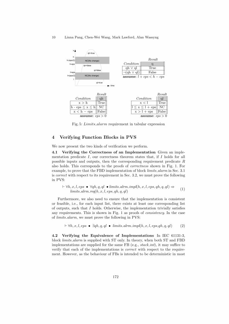
10 Linna Pang, Chen-Wei Wang, Mark Lawford, Alan Wassyng

time

h

h-(eps/2)

qh=true

NC(No change)

l

l+(eps/2)

h-eps

l+eps

qh=false

ql=false

ql=true

NC(No change)

x

ResultCondition q

qh ∨ ql True

¬(qh ∨ ql) False

assume: l + eps < h− eps

ResultCondition qh

x > h True

h - eps ≤ x ≤ h NC

x < h − eps False

assume: eps > 0

ResultCondition ql

x < l True

l ≤ x ≤ l + eps NC

x > l + eps False

assume: eps > 0

Fig. 5: Limits alarm requirement in tabular expression

4 Verifying Function Blocks in PVS

We now present the two kinds of verification we perform.

4.1 Verifying the Correctness of an Implementation Given an imple-mentation predicate I, our correctness theorem states that, if I holds for allpossible inputs and outputs, then the corresponding requirement predicate Ralso holds. This corresponds to the proofs of correctness shown in Fig. 1. Forexample, to prove that the FBD implementation of block limits alarm in Sec. 3.1is correct with respect to its requirement in Sec. 3.2, we must prove the followingin PVS:

` ∀h, x, l, eps • ∀qh, q, ql • limits alrm impl(h, x, l, eps, qh, q, ql)⇒limits alrm req(h, x, l, eps, qh, q, ql)

(1)

Furthermore, we also need to ensure that the implementation is consistentor feasible, i.e., for each input list, there exists at least one corresponding listof outputs, such that I holds. Otherwise, the implementation trivially satisfiesany requirements. This is shown in Fig. 1 as proofs of consistency. In the caseof limits alarm, we must prove the following in PVS:

` ∀h, x, l, eps • ∃qh, q, ql • limits alrm impl(h, x, l, eps,qh, q, ql) (2)

4.2 Verifying the Equivalence of Implementations In IEC 61131-3,block limits alarm is supplied with ST only. In theory, when both ST and FBDimplementations are supplied for the same FB (e.g., stack int), it may suffice toverify that each of the implementations is correct with respect to the require-ment. However, as the behaviour of FBs is intended to be deterministic in most

172

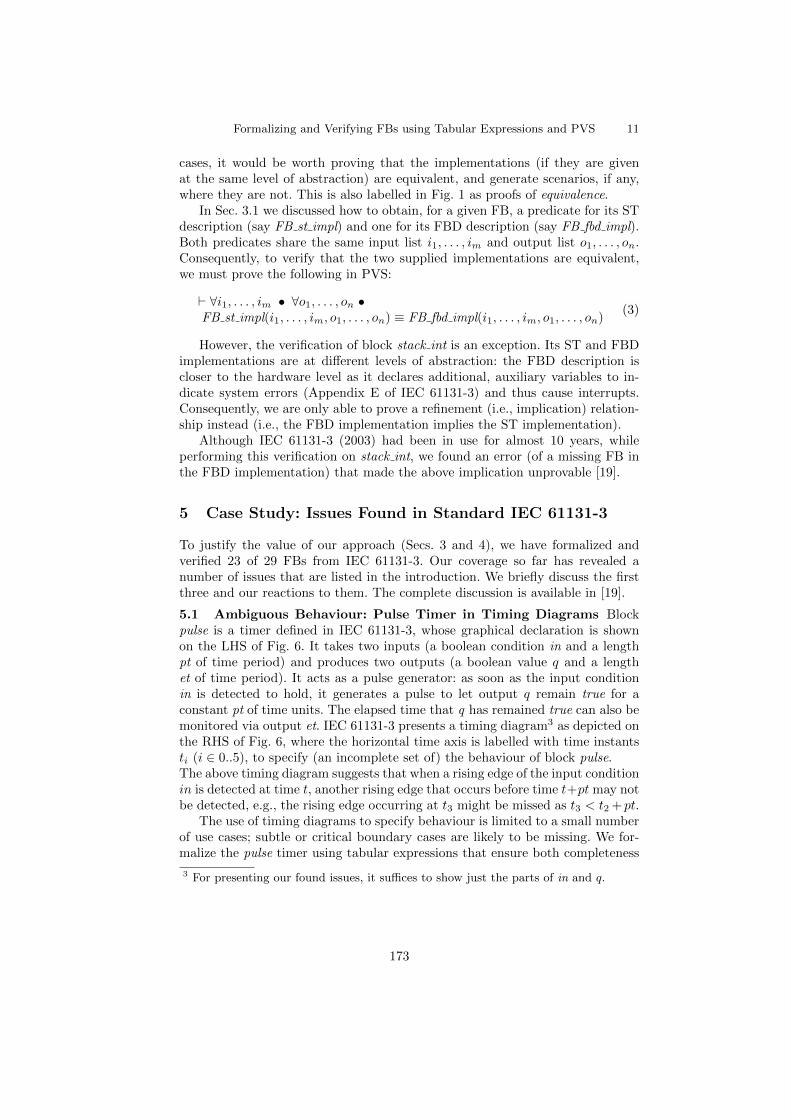
Formalizing and Verifying FBs using Tabular Expressions and PVS 11

cases, it would be worth proving that the implementations (if they are givenat the same level of abstraction) are equivalent, and generate scenarios, if any,where they are not. This is also labelled in Fig. 1 as proofs of equivalence.

In Sec. 3.1 we discussed how to obtain, for a given FB, a predicate for its STdescription (say FB st impl) and one for its FBD description (say FB fbd impl).Both predicates share the same input list i1, . . . , im and output list o1, . . . , on.Consequently, to verify that the two supplied implementations are equivalent,we must prove the following in PVS:

` ∀i1, . . . , im • ∀o1, . . . , on •FB st impl(i1, . . . , im, o1, . . . , on) ≡ FB fbd impl(i1, . . . , im, o1, . . . , on)

(3)

However, the verification of block stack int is an exception. Its ST and FBDimplementations are at different levels of abstraction: the FBD description iscloser to the hardware level as it declares additional, auxiliary variables to in-dicate system errors (Appendix E of IEC 61131-3) and thus cause interrupts.Consequently, we are only able to prove a refinement (i.e., implication) relation-ship instead (i.e., the FBD implementation implies the ST implementation).

Although IEC 61131-3 (2003) had been in use for almost 10 years, whileperforming this verification on stack int, we found an error (of a missing FB inthe FBD implementation) that made the above implication unprovable [19].

5 Case Study: Issues Found in Standard IEC 61131-3

To justify the value of our approach (Secs. 3 and 4), we have formalized andverified 23 of 29 FBs from IEC 61131-3. Our coverage so far has revealed anumber of issues that are listed in the introduction. We briefly discuss the firstthree and our reactions to them. The complete discussion is available in [19].

5.1 Ambiguous Behaviour: Pulse Timer in Timing Diagrams Blockpulse is a timer defined in IEC 61131-3, whose graphical declaration is shownon the LHS of Fig. 6. It takes two inputs (a boolean condition in and a lengthpt of time period) and produces two outputs (a boolean value q and a lengthet of time period). It acts as a pulse generator: as soon as the input conditionin is detected to hold, it generates a pulse to let output q remain true for aconstant pt of time units. The elapsed time that q has remained true can also bemonitored via output et. IEC 61131-3 presents a timing diagram3 as depicted onthe RHS of Fig. 6, where the horizontal time axis is labelled with time instantsti (i ∈ 0..5), to specify (an incomplete set of) the behaviour of block pulse.The above timing diagram suggests that when a rising edge of the input conditionin is detected at time t, another rising edge that occurs before time t+pt may notbe detected, e.g., the rising edge occurring at t3 might be missed as t3 < t2 + pt.

The use of timing diagrams to specify behaviour is limited to a small numberof use cases; subtle or critical boundary cases are likely to be missing. We for-malize the pulse timer using tabular expressions that ensure both completeness

3 For presenting our found issues, it suffices to show just the parts of in and q.

173

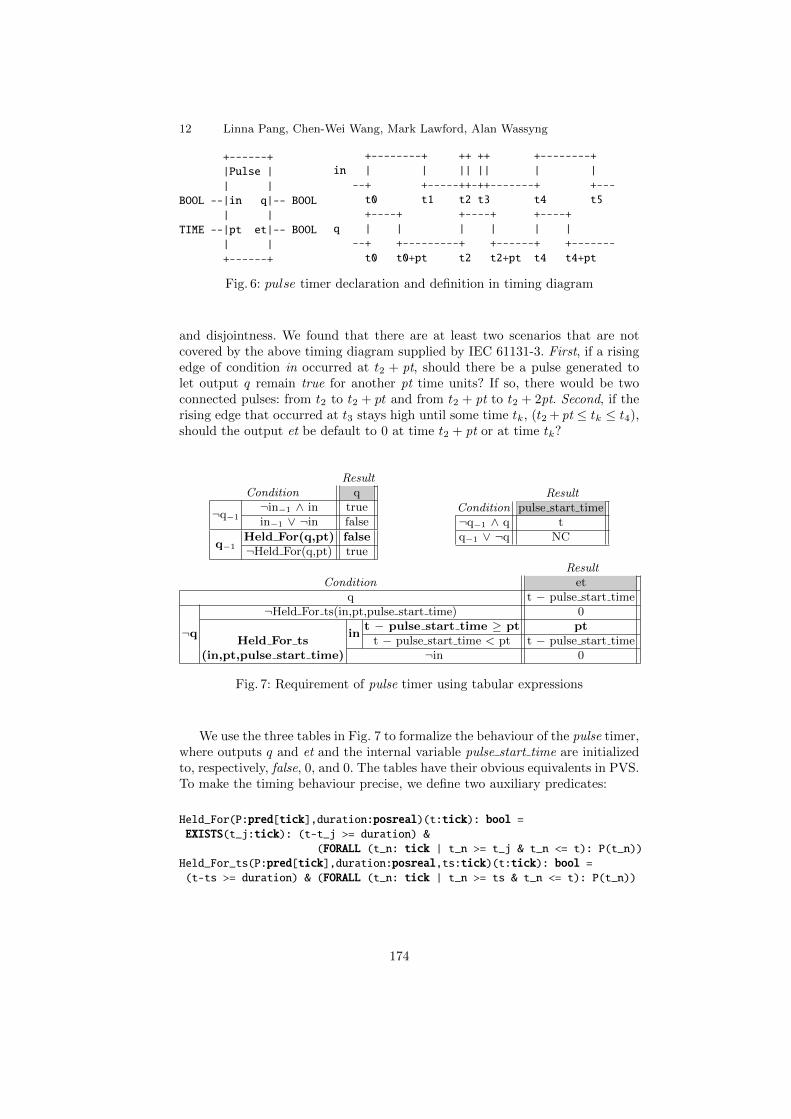
12 Linna Pang, Chen-Wei Wang, Mark Lawford, Alan Wassyng

+------+

|Pulse |

| |

BOOL --|in q|-- BOOL

| |

TIME --|pt et|-- BOOL

| |

+------+

+--------+ ++ ++ +--------+

in | | || || | |

--+ +-----++-++-------+ +---

t0 t1 t2 t3 t4 t5

+----+ +----+ +----+

q | | | | | |

--+ +---------+ +------+ +-------

t0 t0+pt t2 t2+pt t4 t4+pt

Fig. 6: pulse timer declaration and definition in timing diagram

and disjointness. We found that there are at least two scenarios that are notcovered by the above timing diagram supplied by IEC 61131-3. First, if a risingedge of condition in occurred at t2 + pt, should there be a pulse generated tolet output q remain true for another pt time units? If so, there would be twoconnected pulses: from t2 to t2 + pt and from t2 + pt to t2 + 2pt. Second, if therising edge that occurred at t3 stays high until some time tk, (t2 + pt ≤ tk ≤ t4),should the output et be default to 0 at time t2 + pt or at time tk?

ResultCondition q

¬q−1¬in−1 ∧ in truein−1 ∨ ¬in false

q−1Held For(q,pt) false¬Held For(q,pt) true

ResultCondition pulse start time¬q−1 ∧ q tq−1 ∨ ¬q NC

ResultCondition et

q t − pulse start time

¬q¬Held For ts(in,pt,pulse start time) 0

Held For tsin

t − pulse start time ≥ pt ptt − pulse start time < pt t − pulse start time

(in,pt,pulse start time) ¬in 0

Fig. 7: Requirement of pulse timer using tabular expressions

We use the three tables in Fig. 7 to formalize the behaviour of the pulse timer,where outputs q and et and the internal variable pulse start time are initializedto, respectively, false, 0, and 0. The tables have their obvious equivalents in PVS.To make the timing behaviour precise, we define two auxiliary predicates:

Held_For(P:pred[tick],duration:posreal)(t:tick): bool =EXISTS(t_j:tick): (t-t_j >= duration) &

(FORALL (t_n: tick | t_n >= t_j & t_n <= t): P(t_n))Held_For_ts(P:pred[tick],duration:posreal,ts:tick)(t:tick): bool =(t-ts >= duration) & (FORALL (t_n: tick | t_n >= ts & t_n <= t): P(t_n))

174

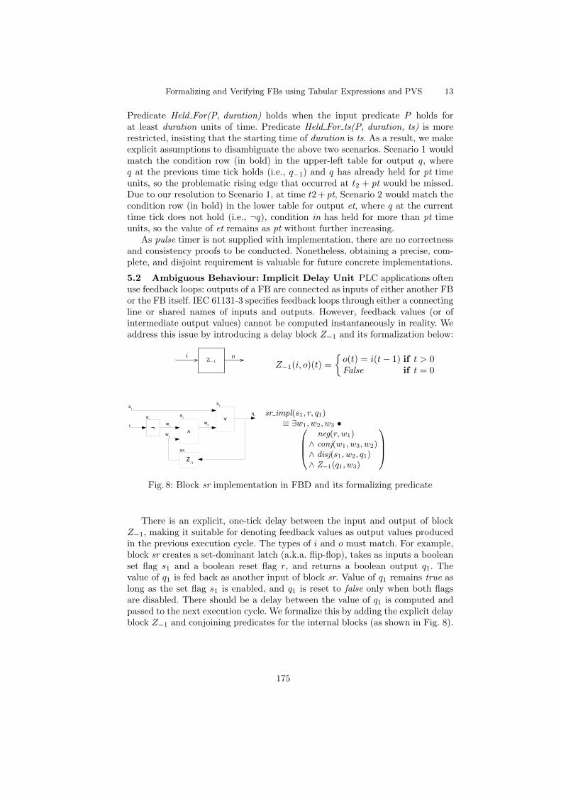
Formalizing and Verifying FBs using Tabular Expressions and PVS 13

Predicate Held For(P, duration) holds when the input predicate P holds forat least duration units of time. Predicate Held For ts(P, duration, ts) is morerestricted, insisting that the starting time of duration is ts. As a result, we makeexplicit assumptions to disambiguate the above two scenarios. Scenario 1 wouldmatch the condition row (in bold) in the upper-left table for output q, whereq at the previous time tick holds (i.e., q−1) and q has already held for pt timeunits, so the problematic rising edge that occurred at t2 + pt would be missed.Due to our resolution to Scenario 1, at time t2 + pt, Scenario 2 would match thecondition row (in bold) in the lower table for output et, where q at the currenttime tick does not hold (i.e., ¬q), condition in has held for more than pt timeunits, so the value of et remains as pt without further increasing.

As pulse timer is not supplied with implementation, there are no correctnessand consistency proofs to be conducted. Nonetheless, obtaining a precise, com-plete, and disjoint requirement is valuable for future concrete implementations.

5.2 Ambiguous Behaviour: Implicit Delay Unit PLC applications oftenuse feedback loops: outputs of a FB are connected as inputs of either another FBor the FB itself. IEC 61131-3 specifies feedback loops through either a connectingline or shared names of inputs and outputs. However, feedback values (or ofintermediate output values) cannot be computed instantaneously in reality. Weaddress this issue by introducing a delay block Z−1 and its formalization below:

Z�1i o

Z−1(i, o)(t) =

{o(t) = i(t− 1) if t > 0False if t = 0

¬˄

˅

Z-1

s1

r

q1

w1

B3

B2B

1

w3

w2

B4

sr impl(s1, r, q1)≡ ∃w1, w2, w3 •

neg(r, w1)∧ conj(w1, w3, w2)∧ disj(s1, w2, q1)∧ Z−1(q1, w3)

Fig. 8: Block sr implementation in FBD and its formalizing predicate

There is an explicit, one-tick delay between the input and output of blockZ−1, making it suitable for denoting feedback values as output values producedin the previous execution cycle. The types of i and o must match. For example,block sr creates a set-dominant latch (a.k.a. flip-flop), takes as inputs a booleanset flag s1 and a boolean reset flag r, and returns a boolean output q1. Thevalue of q1 is fed back as another input of block sr. Value of q1 remains true aslong as the set flag s1 is enabled, and q1 is reset to false only when both flagsare disabled. There should be a delay between the value of q1 is computed andpassed to the next execution cycle. We formalize this by adding the explicit delayblock Z−1 and conjoining predicates for the internal blocks (as shown in Fig. 8).

175

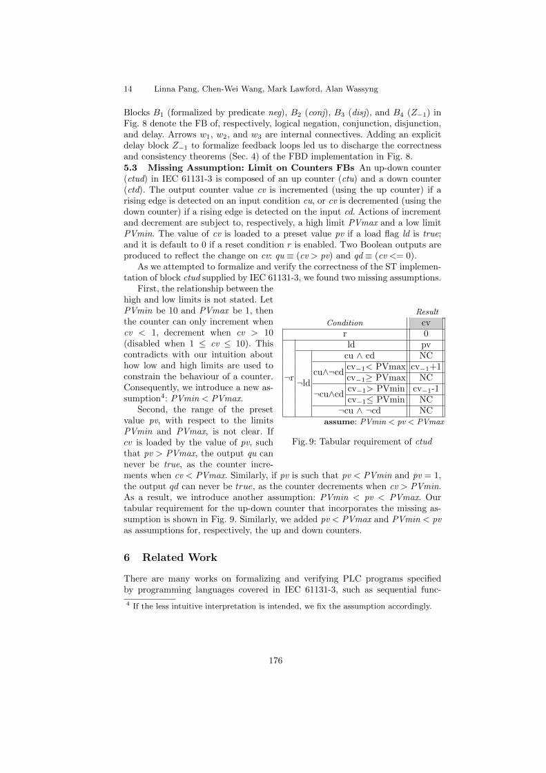
14 Linna Pang, Chen-Wei Wang, Mark Lawford, Alan Wassyng

Blocks B1 (formalized by predicate neg), B2 (conj), B3 (disj), and B4 (Z−1) inFig. 8 denote the FB of, respectively, logical negation, conjunction, disjunction,and delay. Arrows w1, w2, and w3 are internal connectives. Adding an explicitdelay block Z−1 to formalize feedback loops led us to discharge the correctnessand consistency theorems (Sec. 4) of the FBD implementation in Fig. 8.5.3 Missing Assumption: Limit on Counters FBs An up-down counter(ctud) in IEC 61131-3 is composed of an up counter (ctu) and a down counter(ctd). The output counter value cv is incremented (using the up counter) if arising edge is detected on an input condition cu, or cv is decremented (using thedown counter) if a rising edge is detected on the input cd. Actions of incrementand decrement are subject to, respectively, a high limit PVmax and a low limitPVmin. The value of cv is loaded to a preset value pv if a load flag ld is true;and it is default to 0 if a reset condition r is enabled. Two Boolean outputs areproduced to reflect the change on cv: qu ≡ (cv > pv) and qd ≡ (cv <= 0).

As we attempted to formalize and verify the correctness of the ST implemen-tation of block ctud supplied by IEC 61131-3, we found two missing assumptions.

Result

Condition cvr 0

¬r

ld pv

¬ld

cu ∧ cd NC

cu∧¬cdcv−1< PVmax cv−1+1cv−1≥ PVmax NC

¬cu∧cdcv−1> PVmin cv−1-1cv−1≤ PVmin NC

¬cu ∧ ¬cd NCassume: PVmin < pv < PVmax

Fig. 9: Tabular requirement of ctud

First, the relationship between thehigh and low limits is not stated. LetPVmin be 10 and PVmax be 1, thenthe counter can only increment whencv < 1, decrement when cv > 10(disabled when 1 ≤ cv ≤ 10). Thiscontradicts with our intuition abouthow low and high limits are used toconstrain the behaviour of a counter.Consequently, we introduce a new as-sumption4: PVmin < PVmax.

Second, the range of the presetvalue pv, with respect to the limitsPVmin and PVmax, is not clear. Ifcv is loaded by the value of pv, suchthat pv > PVmax, the output qu cannever be true, as the counter incre-ments when cv < PVmax. Similarly, if pv is such that pv < PVmin and pv = 1,the output qd can never be true, as the counter decrements when cv > PVmin.As a result, we introduce another assumption: PVmin < pv < PVmax. Ourtabular requirement for the up-down counter that incorporates the missing as-sumption is shown in Fig. 9. Similarly, we added pv < PVmax and PVmin < pvas assumptions for, respectively, the up and down counters.

6 Related Work

There are many works on formalizing and verifying PLC programs specifiedby programming languages covered in IEC 61131-3, such as sequential func-

4 If the less intuitive interpretation is intended, we fix the assumption accordingly.

176

Formalizing and Verifying FBs using Tabular Expressions and PVS 15

tion charts (SFCs). Some approaches choose the environment of model checking:e.g., to formalize a subset of the language of instruction lists (ILs) using timedautomata, and to verify real-time properties in Uppaal [15]; to automaticallytransform SFC programs into the synchronous data flow language of Lustre,amenable to mechanized support for checking properties [12]; to transform FBDspecifications to Uppaal formal models to verify safety applications in the in-dustrial automation domain [23]; to provide the formal operational semanticsof ILs which is encoded into the symbolic model checker Cadence SMV, andto verify rich behavioural properties written in linear temporal logic (LTL) [5];and to provide the formal verification of a safety procedure in a nuclear powerplant (NPP) in which a verified Coloured Petri Net (CPN) model is derived byreinterpretation from the FBD description [17]. There is also an integration ofSMV and Uppaal to handle, respectively, untimed and timed SFC programs [2].

Some other approaches adopt the verification environment of a theoremprover: e.g., to check the correctness of SFC programs, automatically gener-ated from a graphical front-end, in Coq [3]; and to formalize PLC programsusing higher-order logic and to discharge safety properties in HOL [24]. Theseworks are similar to ours in that PLC programs are formalized and supportedfor mechanized verifications of implementations. An algebra approach for PLCprograms verification is presented in [22]. In [14], a trace function method (TFM)based approach is presented to solve the same problem as ours.

Our work is inspired by [16] in that the overall system behaviour is defined bytaking the conjunction of those of internal components (circuits in [16] or FBs inour case). Our resolutions to the timing issues of the pulse timer are consistentwith [11]. However, our approach is novel in that 1) we also obtain tabularrequirements to be checked against, instead of writing properties directly for thechosen theorem prover or model checker; and 2) our formalization makes it easierto comprehend and to reason about properties of disjointness and completeness.

7 Conclusion and Future Work

We present an approach to formalizing and verifying function blocks (FBs) usingtabular expressions and PVS. We identified issues concerning ambiguity, missingassumptions, and erroneous implementations in the IEC 61131-3 standard ofFBs. As future work, we will apply the same approach to the remaining FBs inIEC 61131, and possibly to IEC 61499 that fits well with distributed systems.

References

1. Bakhmach, E., O.Siora, Tokarev, V., Reshetytskyi, S., Kharchenko, V., Bezsalyi,V.: FPGA - based technology and systems for I&C of existing and advanced reac-tors. International Atomic Energy Agency p. 173 (2009), IAEA-CN-164-7S04

2. Bauer, N., Engell, S., Huuck, R., Lohmann, S., Lukoschus, B., Remelhe, M., Sturs-berg, O.: Verification of PLC programs given as sequential function charts. In:Integration of Software Specification Techniques for Applications in Engineering,LNCS, vol. 3147, pp. 517–540. Springer Berlin Heidelberg (2004)

177

16 Linna Pang, Chen-Wei Wang, Mark Lawford, Alan Wassyng

3. Blech, J.O., Biha, S.O.: On formal reasoning on the semantics of PLC using Coq.CoRR abs/1301.3047 (2013)

4. Camilleri, A., Gordon, M., Melham, T.: Hardware verification using higher-orderlogic. Tech. Rep. UCAM-CL-TR-91, Cambridge Univ. Computer Lab (1986)

5. Canet, G., Couffin, S., Lesage, J.J., Petit, A., Schnoebelen, P.: Towards the auto-matic verification of plc programs written in instruction list. In: IEEE InternationalConference on Systems, Man and Cybernetics. pp. 2449–2454 (2000)

6. Eles, C., Lawford, M.: A tabular expression toolbox for Matlab/Simulink. In:NASA Formal Methods. pp. 494–499 (2011)

7. Hu, X., Lawford, M., Wassyng, A.: Formal verification of the implementability oftiming requirements. In: FMICS. LNCS, vol. 5596, pp. 119–134. Springer (2009)

8. IEC: 61131-3 Ed. 2.0 en:2003: Programmable Controllers — Part 3: ProgrammingLanguages. International Electrotechnical Commission (2003)

9. IEC: 61131-3 Ed. 3.0 en:2013: Programmable Controllers — Part 3: ProgrammingLanguages. International Electrotechnical Commission (2013)

10. Jin, Y., Parnas, D.L.: Defining the meaning of tabular mathematical expressions.Science of Computer Programming 75(11), 980 – 1000 (2010)

11. John, K.H., Tiegelkamp, M.: IEC 61131-3: Programming Industrial AutomationSystems Concepts and Programming Languages, Requirements for ProgrammingSystems, Decision-Making Aids. Springer, 2nd edn. (2010)

12. Kabra, A., Bhattacharjee, A., Karmakar, G., Wakankar, A.: Formalization of se-quential function chart as synchronous model in Lustre. In: NCETACS. pp. 115–120 (2012)

13. Lawford, M., McDougall, J., Froebel, P., Moum, G.: Practical application of func-tional and relational methods for the specification and verification of safety criticalsoftware. In: Proc. of AMAST 2000. LNCS, vol. 1816, pp. 73–88. Springer (2000)

14. Liu, Z., Parnas, D., Widemann, B.: Documenting and verifying systems assembledfrom components. Frontiers of Computer Science in China 4(2), 151–161 (2010)

15. Mader, A., Wupper, H.: Timed automaton models for simple programmable logiccontrollers. In: ECRTS. pp. 114–122. IEEE (1999)

16. Melham, T.: Abstraction mechanisms for hardware verification. In: VLSI Specifica-tion, Verification and Synthesis. pp. 129–157. Kluwer Academic Publishers (1987)

17. Nemeth, E., Bartha, T.: Formal verification of safety functions by reinterpretationof functional block based specifications. In: FMICS, pp. 199–214. Springer (2009)

18. Owre, S., Rushby, J.M., Shankar, N.: PVS: A Prototype Verification System. In:CADE. LNCS, vol. 607, pp. 748–752 (1992)

19. Pang, L., Wang, C.W., Lawford, M., Wassyng, A.: Formalizing and verifying func-tion blocks using tabular expressions and PVS. Tech. Rep. 11, McSCert (Aug 2013)

20. Parnas, D.L., Madey, J.: Functional documents for computer systems. Science ofComputer Programming 25(1), 41–61 (1995)

21. Parnas, D.L., Madey, J., Iglewski, M.: Precise documentation of well-structuredprograms. IEEE Transactions on Software Engineering 20, 948–976 (1994)

22. Roussel, J.M., Faure, J.: An algebraic approach for PLC programs verification. In:6th International Workshop on Discrete Event Systems. pp. 303–308 (2002)

23. Soliman, D., Thramboulidis, K., Frey, G.: Transformation of function block dia-grams to Uppaal timed automata for the verification of safety applications. AnnualReviews in Control (2012)

24. Volker, N., Kramer, B.J.: Automated verification of function block-based industrialcontrol systems. Science of Computer Programming 42(1), 101 – 113 (2002)

25. Wassyng, A., Janicki, R.: Tabular expressions in software engineering. In: Proceed-ings of ICSSEA’03. vol. 4, pp. 1–46. Paris, France (2003)

178

Parametric Schedulability Analysis of FixedPriority Real-Time Distributed Systems

Youcheng Sun1, Romain Soulat2, Giuseppe Lipari1,2, Etienne Andre3, andLaurent Fribourg2

1 Scuola Superiore Sant’Anna, Pisa, Italy2 LSV, ENS Cachan & CNRS, France

3 Universite Paris 13, Sorbonne Paris Cite, LIPN, CNRS, Villetaneuse, France

Abstract. In this paper, we address the problem of parametric schedu-lability analysis of distributed real-time systems scheduled by fixed pri-ority. We propose two different approaches to parametric analysis. Thefirst one is a novel analytic technique that extends single-processor sen-sitivity analysis to the case of distributed systems. The second approachis based on model checking of Parametric Stopwatch Automata (PSA):we generate a PSA model from a high-level description of the system,and then we apply the Inverse Method to obtain all possible behavioursof the system. Both techniques have been implemented in two softwaretools, and they have been compared with classical holistic analysis ontwo meaningful test cases. The results show that the analytic methodprovides results similar to classical holistic analysis in a very efficientway, whereas the PSA approach is slower but covers the entire space ofsolutions.

1 Introduction and motivation

Designing and analysing distributed real-time systems is a very challenging task.The main source of complexity arises from the large number of parameters to con-sider: tasks priorities, computation times and deadlines, synchronisation, prece-dence and communication constraints, etc. Finding the optimal values for theparameters is not easy and often a small change in one parameter may com-pletely change the behaviour of the system and even compromise its correctness.For these reasons, designers are looking for analysis methodologies that allowincremental design and exploration of the parameter space.

Task computation times are particularly important parameters. In modernprocessor architectures, it is very difficult to precisely compute worst-case com-putation times of tasks, thus estimations derived by previous executions are oftenused in the analysis. However, estimations may turn out to be optimistic, hencean error in the estimation of a worst-case execution time may compromise theschedulability of the entire system.

In this paper we investigate the problem of doing parametric analysis of real-time distributed systems scheduled by fixed priority. We consider an application

179

modelled by a set of pipelines (also called transactions in [20]), where eachpipeline is a sequence of periodic tasks to be executed in order, and all tasksin a pipeline must complete before an end-to-end deadline. We consider that allprocessors in the distributed system are connected by one or more CAN bus [13],a network standard used in automotive applications.

The first contribution of the paper (Section 4) is to propose a new methodfor doing parametric analysis of the system, using the worst-case computationtimes of the tasks as parameters. The method extends the sensitivity analysisproposed by Bini et al. [9] by considering distributed systems and non-preemptivescheduling.

The proposed analytical method is not exact, as it sometimes overestimatesthe interference of higher priority tasks and of previous tasks in the pipelineon the response time of a task. Therefore, the second contribution of the paper(Section 5) is to propose also an exact schedulability analysis by modelling adistributed real-time system as a set of parametric timed automata; then weapply a model checking methodology using the Inverse Method [7, 14].

Finally, in Section 6 we compare these two approaches with the Mast tool[16, 17], a state-of the art tool for classical schedulability analysis. Comparison isperformed on two case studies from the research literature on which we measuredrun-time and effectiveness of the three analyses. Results show that the analyticalapproach can very efficiently compute the feasible space of parameters with agood precision.

2 Related Work

Many research papers have already addressed the problem of parametric schedu-lability analysis, especially on single processor systems. Bini and Buttazzo [9]proposed an analysis of fixed priority single processor systems, which is used asa basis for this paper.

Parameter sensitivity can be also be carried out by repeatedly applying clas-sical schedulability tests, like the holistic analysis [20]. One example of this ap-proach is used in the Mast tool [16], in which it is possible to compute the slack(i.e. the percentage of variation) with respect to one parameter for single pro-cessor and for distributed systems by applying binary search in that parameterspace [20].

A similar approach is followed by the SymTA/S tool [18], which is basedon the event-stream model [21]. Another interesting approach is the ModularPerformance Analysis (MPA) [24], which is based on Real-Time Calculus. Inboth cases, the analysis is compositional, therefore less complex than the holisticanalysis. Nevertheless, these approaches are not fully parametric, in the sensethat it is necessary to repeat the analysis for every combination of parametervalues in order to obtain the schedulability region.

Model checking of parametric timed automata (PTA) or parametric stop-watch automata (PSA) can be used for parametric schedulability analysis [12].In particular, thanks to generality of the PTA and PSA modelling language, it is

180

possible to model a larger class of constraints, and perform parametric analysison many different variables, for example task offsets. This approach has beenrecently extended to distributed real-time systems [19].

Also grounded on PTA and PSA is the Inverse Method [7], applied in par-ticular to schedulability analysis [14]. This method is very general because itpermits to perform analysis on any system parameter. However, this generalitymay be paid in terms of complexity of the analysis.

In this paper, we aim at performing fully parametric analysis of real-timedistributed systems. We first present extensions of the methods proposed in [9] tothe case of distributed real-time systems. We also present a model of a distributedreal-time systems using PSA, and compare the two approaches against classicalanalysis in Mast.

3 System Model

We consider distributed real-time systems consisting of several computationalnodes, each one hosting one single processor, which are connected by one ormore shared networks. Without loss of generality, from now on we will use theterm task to denote both tasks and messages, and the term processor to denoteboth processors and networks.

A distributed real-time system consists of a set of task pipelines {P1, . . . ,Pn}to be executed on a set of processors. A pipeline is a chain of tasks Pj ={τ j1 , . . . , τ jn} to be executed in order, and each task is allocated on one (pos-sibly different) processor. In order to simplify the notation, in the following wesometimes drop the pipeline superscript when there is no possibility of misinter-pretation.

A pipeline is assigned two fixed parameters: T j is the pipeline period andDje2e is the end-to-end deadline. This means that all tasks of the pipeline are

activated together every T j units of time; and all tasks should be completedwithin a time interval of Dj

e2e.A task in the pipeline can be a piece of code to be executed on a processor

or a message to be sent over a network. More precisely, a real-time periodic taskis a tuple τi = (Ci, Ti, Di, Ri, qi, pi, Ji).

This task model contains the following fixed parameters:

– Ti is the task period. All tasks in the same pipeline have period equal to thepipeline period T ;

– Di is the task relative deadline;– qi is the task priority; the larger qi, the higher the priority;– pi is the index of the processor (or network) on which the task executes.

Also, a task is characterised by the following free parameters (variables):

– Ci is the worst-case computation time (or worst-case transmission time, incase it models a message). It is the worst-case time the task needs to com-plete one periodic instance when executed alone on a dedicated processor

181

(or network). In this paper we want to characterise the schedulability of adistributed system in the space of the computation times, so Ci is a freeparameter.

– Ri is the task worst-case response time, i.e. the worst case finishing time ofany task instance relative to the activation of its pipeline.

– Ji is the task worst-case activation jitter, i.e. the greatest time since itsactivation that a task must wait for all preceding tasks to complete theirexecution.

Every task activation is an instance (or job) of the task. We denote the kthinstance of task τi as τi,k. An instance τi,k of a task in the pipeline can startexecuting only after the corresponding instance of the preceding task τi−1,k hascompleted. Finally, the last task in the pipeline must complete every instancebefore De2e units of time from its pipeline’s activation. For a job τi,k we definethe following notation:

– ai,k is τi,k’s arrival time (coincident with the activation time of the pipeline).– si,k is the start time of the instance, i.e. the first time the instance executes

on the processor.– fi,k is the job’s finishing time.– ri,k the task release time. The first task of a pipeline is released immediately

at the time of its arrival r0,k = a0,k; successive tasks are released at thefinishing time of the preceding tasks: ri,k = fi−1,k. The following relationshipholds: ∀i, k a0,k = ai,k ≤ ri,k ≤ si,k < fi,k

– The maximum difference between arrival and release time is the worst-caseactivation jitter of the task: Ji = maxk(ri,k − ai,k).

– The maximum difference between finishing time and arrival time is the worst-case response time of the task: Ri = maxk(fi,k − ai,k).

Parameters Ri and Ji depend on the other tasks parameters and on the schedul-ing policy according to a complex set of equations. Of course, they cannot beconsidered parameters that the programmer can modify: nevertheless, for ourpurposes it is useful to consider them as variables to help us write the set ofconstraints that define the schedulability space (the exact role of such variableswill be detailed in Section 4.3).

A scheduling algorithm is fully preemptive if the execution of a lower priorityjob can be suspended at any instant by the release of a higher priority job,which is then executed in its place. A scheduling algorithm is non-preemptive ifa lower priority job, once it has started executing, can complete its executionregardless of the release of higher priority jobs. In this paper, we consider fullypreemptive fixed priority scheduling for processors, and non-preemptive fixedpriority scheduling for networks.

4 Analytic Method

In this section we present a novel method for parametric analysis of distributedsystem. The method extends the sensitivity analysis by Bini et al. [22, 9] toinclude jitter and deadline parameters.

182

In Sections 4.1 and 4.2, we only consider the scheduling of independent peri-odic tasks in a single processor. Then, in Section 4.3, we extend the schedulabilityanalysis to distributed systems.

4.1 Preemptive Tasks with Constrained Deadlines

There are many ways to test the schedulability of a set of real-time periodictasks scheduled by fixed priority on a single processor. In the following, we willuse the test proposed by Seto et al. [22] because it is amenable to parametricanalysis of computation times, jitters and deadlines.

The original theorem was formulated for tasks with deadlines equal to peri-ods. For the moment, we generalise it to tasks with constrained deadlines (i.e.Di ≤ T ), while in Section 4.2 we deal with unconstrained deadlines, jitter andnon-preemptive scheduling.

Definition 1. The set of scheduling points Pi−1(t) for a task τi is the set of allvectors corresponding to multiples of the period of any task τj with priority higherthan τi, until the maximum possible value of the deadline. It can be computed as

follows. Let ηj(t) =⌈tTj

⌉, and let ηi−1(t) be the corresponding vector of i − 1

elements with j = 0, . . . , i− 1. Then:

Pi−1(t) = {ηi−1(t)} ∪ {ηi−1(kTh) | 0 < kTh < t, h < i} (1)

Theorem 1 ([22]). Consider a system of periodic tasks {τ1, . . . , τn} with con-strained deadlines and zero jitter, executed on a single processor by a fixed pri-ority preemptive scheduler. Assume all tasks are ordered in decreasing order ofpriorities, with τ1 being the highest priority task.

Task τi is schedulable if and only if:

∃n ∈ Pi−1(Di)

Ci +i−1∑

j=1

njCj ≤ nkTk ∀k = 1, . . . , i− 1

Ci +i−1∑

j=1

njCj ≤ Ri

Ri ≤ Di

(2)

where n is a vector of i−1 integers, and Pi−1(Di) is the set of scheduling points.

Notice that, with respect to the original formulation, we have separated the caseof k = i from the rest of the inequalities and we introduced variable Ri.

The theorem allows us to only consider sets of linear inequalities, becausethe non-linearity has been encoded in the variables nj . Each vector n definesa convex region (maybe empty) with variables C1, . . . , Ci and R1, . . . , Ri. The“exists” quantifier means that the region for each task τi is the union of convexregions, hence it may be non-convex. Since we have to check the schedulability of

183

all tasks, we must intersect all such regions to obtain the final region of schedu-lable parameters. The resulting system is a disjunction of sets of conjunctions ofinequalities. Geometrically, this corresponds to a non-convex polyhedron in thespace of the variables C and R of tasks.

It is worth to note that, using this formulation, we can compute the responsetime of a task by simply minimising the corresponding variable Ri under theconstraints of Equation (2). As an example, consider the following task set (thesame as in [10]): τ1 = (C = 1, T = 3), τ2 = (C = 2, T = 8), τ3 = (C = 4, T = 20),in decreasing order of priority, to be scheduled by preemptive fixed priorityscheduling on a single processor.

We consider the response time R3 as a parameter and set up the system ofinequalities according to Equation (2). After reduction of the non-useful con-straints, we obtain 12 ≤ R3 ≤ 20. Therefore, the response time is R3 = 12,which is the same that can be obtained by classical response time analysis.

4.2 Extensions to the Model

We now extend Seto’s test to unconstrained deadlines and variable jitters, andnon-preemptive scheduling. Non-preemptive scheduling can be modelled by con-sidering an initial blocking time, due to the fact that a task cannot preemptlower-priority executing tasks.

The worst case response time for a non preemptive task τi can be found inits longest i-level active period [11]. An i-level active period Li is an interval[a, b) such that the amount of processing that needs to be performed due tojobs with priority higher than or equal to τi (including τi itself) is larger than0 for all t ∈ (a, b), and equal to 0 at instants a and b. The longest Li can befound by computing the lowest fixed point of a recursive function. Notice that,by considering non-preemption and tasks with deadline greater than periods, theworst-case response time may be found in any instance of the active period, notnecessarily in the first one (as with the classical model of constrained deadlinepreemptive tasks).

Unfortunately, the longest busy period cannot be computed when tasks haveparametric worst-case computation times. However, under the assumption thatthere is at least an idle-time in the hyperperiod (i.e. its utilisation is strictly lessthan 100%) a sufficient feasibility test can be derived by computing the worst-case response time for every instance of the task set in the hyperperiod Hn.Therefore, we can extend our model as follows.

Theorem 2. A non preemptive task τi is schedulable if ∀h = 1, . . . , HnTi , ∃n ∈Pi−1((h− 1)Ti +Di) such that

– Bi + (h− 1)Ci +i−1∑j=1

njCj ≤ nlTl − Jl ∀l = 1, . . . , i− 1;

– Bi + (h− 1)Ci +i−1∑j=1

njCj ≤ (h− 1)Ti +Ri − Ci − Ji;– Ri ≤ Di and Bi ≤ Cj − 1 for all j > i.

184

Proof. See [23].

Term Bi is an additional internal variable used to model the blocking time thata task suffers from lower priority tasks. It is possible to avoid the introductionof this additional variable by substituting it in the inequalities with a simpleFourier-Motzkin elimination.

Notice that the introduction of unconstrained deadlines adds a great amountof complexity to the problem. In particular, the number of non-convex regions tointersect is now O(

∑ni=1

HnTi

), which is dominated by O(nHn). So, the proposedproblem representation is pseudo-polynomial in the size of the hyperperiod. How-ever, in real applications, we expect the periods to have “nice” relationships: forexample, in many cases engineers choose periods that are multiples of each oth-ers. Therefore, we expect the set of inequalities to have manageable size forrealistic problems.

4.3 Distributed Systems

Until now, we have considered the parametric analysis of independent tasks onsingle processor systems, with computation times, response times, blocking timesand jitters as free variables.

One key observation is that a precedence constraint between two consecutivetasks τi and τi+1 in the same pipeline can be expressed as Ri ≤ Ji+1. Thisrelationship derives directly from the definition of response time and jitter inSection 3. Using this elementary property, we can now build the parametricspace for a distributed system as follows.

1. For each processor and network, we build the constraint system of Theo-rem 2. Notice that the set of constraints for the individual single processorsystems are independent of each other (because they are constraints on dif-ferent tasks).

2. For each pipeline Pa:– two successive tasks τai and τai+1 must fulfil the constraint Rai ≤ Jai+1;– for the initial task we impose Ja1 = 0.

Such pipeline constraints must intersect the combined system to producethe final system of constraints. However, simply adding the above precedenceconstraints can lead to pessimistic solutions. In fact, if two tasks from the samepipeline are assigned to the same processor, the interference they may cause oneach other and on the other tasks may be limited.

Suppose τai and τaj are allocated to the same processor and qai > qaj . Then,τai can at most interfere with the execution of a job from τaj a number of times

equal to ξ =⌈max{0,Dae2e−Ta}

Ta

⌉. So, we impose that ∀n ∈ Pj−1, ni ≤ ξ.

The analytic method proposed in this section has been implemented in asoftware tool, called RTScan, which is based on the PPL (Parma PolyhedraLibrary) [8], a library specifically designed and optimised to represent and op-erate on polyhedra. The library efficiently operates on rational numbers with

185

arbitrary precision: therefore, in this work we make the assumption that all vari-ables (computations times, response times and jitter) are defined in the domainof rationals (rather than reals).

We observed that the complexity of the methodology for generating the pa-rameter space strongly depends on the number of free parameters considered inthe analysis. Therefore, as a preliminary step, the tool requires the user to se-lect a subset of the computation times on which the analysis will be performed,whereas the other parameters will be assigned fixed values. During constructionof the polyhedron we have to keep Ri, Ji and Bi for each task as variables.Therefore, the number of variables to be managed is nV = 4 ·N + F , where Nis the number of tasks and F is the number of variables to analyse. At the end,we can eliminate the Ri, Ji and Bi variables, hence the final space consists ofF dimensions. An evaluation of this tool and of the run-time complexity of theanalysis will be presented in Section 6.

The analytic method described so far is not exact. In fact, when dealing withpipelines in a distributed system we may sometimes overestimate the interferenceof higher priority-tasks on lower priority ones. For this reason, we now presentan exact parametric analysis based on PSA and model checking.

5 The Inverse Method Approach

5.1 Parametric Timed Automata with Stopwatches

Timed automata are finite-state automata augmented with clocks, i.e., real-valued variables increasing uniformly, that are compared within guards and in-variants with timing delays [3]. Parametric timed automata (PTA) [4] extendtimed automata with parameters, i.e., unknown constants, that can be used inguards and invariants. We will use here an extension of PTA with stopwatches [2],where clocks can be stopped in some control states of the automaton.

Given a set X of clocks and a set U of parameters, a constraint C over Xand U is a conjunction of linear inequalities on X and U1. Given a parametervaluation (or point) π, we write π |= C when the constraint where all parameterswithin C have been replaced by their value as in π is satisfied by a non-emptyset of clock valuations.

Definition 2. A parametric timed automaton with stopwatches (PSA) A is(Σ,Q, q0, X, U,K, I, slope,→) with Σ a finite set of actions, Q a finite set oflocations, q0 ∈ Q the initial location, X a set of h clocks, U a set of parameters,K a constraint over U , I the invariant assigning to every q ∈ Q a constraintover X and U , slope : Q→ {0, 1}h assigns a constant slope to every location, and→ a step relation consisting of elements (q, g, a, ρ, q′), where q, q′ ∈ Q, a ∈ Σ,ρ ⊆ X is the set of clocks to be reset, and the guard g is a constraint over Xand U .1 Note that this is a more general form than the strict original definition of PTA [4];

since most problems for PTA are undecidable anyway, this has no practical incidence,and increases the expressiveness of the formalism.

186

The semantics of a PSA A is defined in terms of states, i.e., pairs (q, C)where q ∈ Q and C is a constraint over X and U . Given a point π, we saythat a state (q, C) is π-compatible if π |= C. Runs are alternating sequences ofstates and actions, and traces are time-abstract runs, i.e., alternating sequencesof locations and actions. The trace set of A corresponds to the traces associatedwith all the runs of A. Given A and π, we denote by A[π] the (non-parametric)timed stopwatch automaton where each occurrence of a parameter has beenreplaced by its constant value as in π. Details can be found in, e.g., [7].

The Inverse Method for PSA [7] exploits the knowledge of a reference point oftiming values for which the good behaviour of the system is known. The methodsynthesises automatically a dense space of points around the reference point, forwhich the discrete behaviour of the system, that is the set of all the admissiblesequences of interleaving events, is guaranteed to be the same.

The Inverse Method IM proceeds by exploring iteratively longer runs fromthe initial state. When a π-incompatible state is met (that is a state (q, C) suchthat π 6|= C), a π-incompatible inequality J is selected within the projectionof C onto U . This inequality is then negated, and the analysis restarts with amodel further constrained by ¬J . When a fixpoint is reached, that is when noπ-incompatible state is found and all states have their successors within the setof reachable states, the intersection of all the constraints onto the parameters isreturned.

Although the principle of IM shares similarities with sensitivity analysis, IMproceeds by iterative state space exploration. Furthermore, its result comes underthe form of a fully parametric constraint, in contrast to sensitivity analysis. Byrepeatedly applying the method, we are able to decompose the parameter spaceinto a covering set of “tiles”, which ensure a uniform behaviour of the system:it is sufficient to test only one point of the tile in order to know whether or notthe system behaves correctly on the whole tile. This is known as the behaviouralcartography [5].

5.2 Modelling the System Using Parametric Stopwatch Automata

Timed Automata with Stopwatches have been used for modelling schedulingproblems in the past. Our model technique is similar to [2, 1], except that wemodel pipelines of tasks, and that we use PSA for obtaining the space of feasiblecomputation times. In the current implementation, we only model pipelines withend-to-end deadlines no larger than their periods. This allows us to simplify themodel and reduce the complexity of the analysis. The extension to deadlineslarger than the period is discussed at the end of the section.

We illustrate our model with the help of an example of two pipelines P1,P2

with P1 = {τ1, τ2}, P2 = {τ3, τ4}, p(τ1) = p(τ4) = p1, p(τ2) = p(τ3) = p2,p1 being a preemptive processor and p2 being non-preemptive. We have thatq1 > q4 and q3 > q2.

Figure 1 shows the PSA model of a pipeline. A pipeline is a sequence of tasksthat are to be executed in order: when a task completes its instance, it instantlyreleases the next task in the pipeline. Since we assume constrained deadlines,

187

once every task in the pipeline has completed, the pipeline waits for the nextperiod to start. This PSA contains one local clock xP1 , one parameter T1 (thepipeline’s period), and synchronises on 5 actions: “τ1 release”, “τ1 completed”,“τ2 release”, “τ2 completed”, and “P1 restart”. The order of these events imposesthat task τ1 must be entirely executed before task τ2. The initialisation of thepipeline’s local clock xP1 and the invariant xP1 ≤ T1 ensure that the pipeline’sexecution terminates within its period T1. The guard xP1 == T1 ensures thatthe pipeline restarts after exactly T1 units of time.

τ1 waitingurgent

τ1 released

τ2 waitingurgent

τ2 releasedP1 completexP1 ≤ T1

τ1 release

τ1 completed

τ2 release

τ2 completed

xP1 == T1

P1 restartxP1 := 0

Fig. 1. PSA modelling a pipeline P1 with two tasks τ1, τ2

Figure 2 shows the model of a preemptive processor with 2 tasks τ1 and τ4,where task τ1 has higher priority over task τ4. The processor starts by beingidle, waiting for a task release. As soon as a request has been received (e.g.action “τ4 release”), it moves to one of the states where the corresponding taskis running (“τ4 running”). If it receives another release request (“τ1 release”),it moves to the state corresponding to the higher priority task running (“τ1release, τ4 released”). The fact that τ1 does not execute anymore is modelled bythe blocking of the clock xτ4 corresponding to task τ4. Moreover, while a taskexecutes, the scheduler automaton checks if the corresponding pipeline missesits deadline (e.g. guard xP1 > D1

e2e, where D1e2e is τ1’s deadline). In the case of a

deadline miss, the processor moves to a special failure state (“deadline missed”)and stops any further computation.

The model of a non-preemptive processor is very similar to the model ofpreemptive processor: the central state in Figure 2 which accounts for the factthat τ4 is stopped when τ1 is released, in the non-preemptive case must not stopτ4, but simply remember that τ1 has been released, so that we can move to thetop state when τ4 completes its instance.

We use the Imitator software tool [6] implementing the behavioural car-tography, to perform the analysis of the PSA. The tool takes as input a textualdescription of the PSA and an interval of values for each parameter, which canbe seen as a hypercube in |U | dimensions, with |U | the number of parameters.Then, it explores the hypercube of values using IM , and it outputs a set of tiles.

For each tile, Imitator derives whether the corresponding system behaviouris valid (i.e. no deadline miss is present), which corresponds to a good tile,or invalid (at least one deadline miss has been found), which corresponds toa bad tile. Every behaviour can be regarded as a set of traces of the system.

188

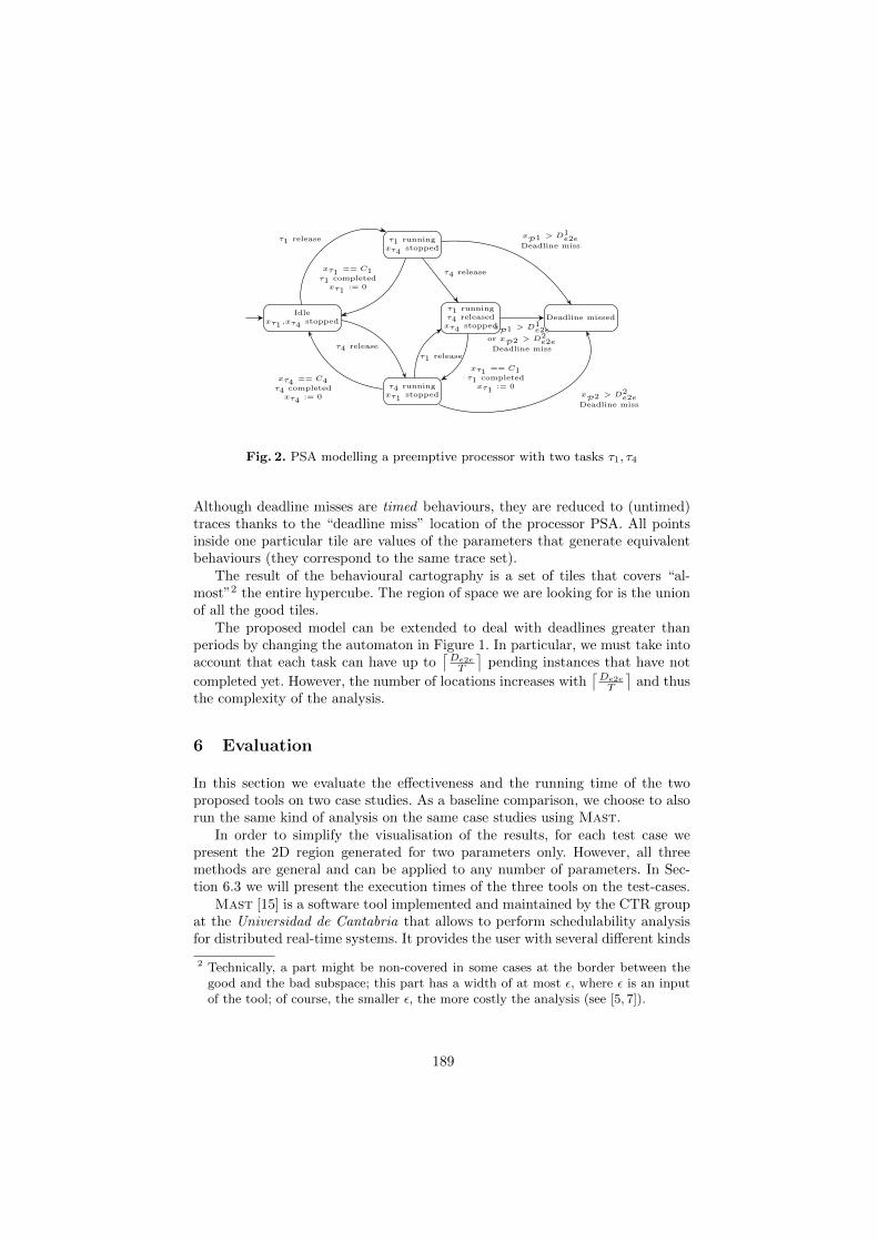
Idlexτ1 ,xτ4 stopped

τ1 runningxτ4

stopped

τ4 runningxτ1

stopped

τ1 runningτ4 releasedxτ4

stoppedDeadline missed

τ1 release

τ4 release

xτ1== C1

τ1 completedxτ1 := 0

τ4 release

xP1 > D1e2e

Deadline miss

xτ4 == C4τ4 completedxτ4

:= 0

τ1 release

xP2 > D2e2e

Deadline miss

xτ1 == C1τ1 completedxτ1

:= 0

xP1 > D1e2e

or xP2 > D2e2e

Deadline miss

Fig. 2. PSA modelling a preemptive processor with two tasks τ1, τ4

Although deadline misses are timed behaviours, they are reduced to (untimed)traces thanks to the “deadline miss” location of the processor PSA. All pointsinside one particular tile are values of the parameters that generate equivalentbehaviours (they correspond to the same trace set).

The result of the behavioural cartography is a set of tiles that covers “al-most”2 the entire hypercube. The region of space we are looking for is the unionof all the good tiles.

The proposed model can be extended to deal with deadlines greater thanperiods by changing the automaton in Figure 1. In particular, we must take intoaccount that each task can have up to

⌈De2eT

⌉pending instances that have not

completed yet. However, the number of locations increases with⌈De2eT

⌉and thus

the complexity of the analysis.

6 Evaluation

In this section we evaluate the effectiveness and the running time of the twoproposed tools on two case studies. As a baseline comparison, we choose to alsorun the same kind of analysis on the same case studies using Mast.

In order to simplify the visualisation of the results, for each test case wepresent the 2D region generated for two parameters only. However, all threemethods are general and can be applied to any number of parameters. In Sec-tion 6.3 we will present the execution times of the three tools on the test-cases.

Mast [15] is a software tool implemented and maintained by the CTR groupat the Universidad de Cantabria that allows to perform schedulability analysisfor distributed real-time systems. It provides the user with several different kinds

2 Technically, a part might be non-covered in some cases at the border between thegood and the bad subspace; this part has a width of at most ε, where ε is an inputof the tool; of course, the smaller ε, the more costly the analysis (see [5, 7]).

189

Table 1. Test case 1; all numbers in“ticks”

Pipeline/Task T De2e Tasks C q p

τ1 20 20 – free 9 1

P 1 150 150

τ11 free 3 1τ12 10 9 2τ13 8 5 3τ14 15 2 2τ15 25 2 1

τ2 30 30 – 6 9 3

τ3 200 200 – 40 2 3

0

5

10

15

20

0 10 20 30 40 50 60 70 80 90

C1

C1

1

0

5

10

15

20

0 10 20 30 40 50 60 70 80 90

C1

C1

1

0

5

10

15

20

0 10 20 30 40 50 60 70 80 90

C1

C1

1

0

5

10

15

20

0 10 20 30 40 50 60 70 80 90

C1

C1

1

0

5

10

15

20

0 10 20 30 40 50 60 70 80 90

C1

C1

1

0

5

10

15

20

0 10 20 30 40 50 60 70 80 90

C1

C1

1

0

5

10

15

20

0 10 20 30 40 50 60 70 80 90

C1

C1

1

0

5

10

15

20

0 10 20 30 40 50 60 70 80 90

C1

C1

1

0

5

10

15

20

0 10 20 30 40 50 60 70 80 90

C1

C1

1

0

5

10

15

20

0 10 20 30 40 50 60 70 80 90

C1

C1

1

0

5

10

15

20

0 10 20 30 40 50 60 70 80 90

C1

C1

1

0

5

10

15

20

0 10 20 30 40 50 60 70 80 90

C1

C1

1

0

5

10

15

20

0 10 20 30 40 50 60 70 80 90

C1

C1

1

0

5

10

15

20

0 10 20 30 40 50 60 70 80 90

C1

C1

1

0

5

10

15

20

0 10 20 30 40 50 60 70 80 90

C1

C1

1

0

5

10

15

20

0 10 20 30 40 50 60 70 80 90

C1

C1

1

0

5

10

15

20

0 10 20 30 40 50 60 70 80 90

C1

C1

1

0

5

10

15

20

0 10 20 30 40 50 60 70 80 90

C1

C1

1

0

5

10

15

20

0 10 20 30 40 50 60 70 80 90

C1

C1

1

0

5

10

15

20

0 10 20 30 40 50 60 70 80 90

C1

C1

1

0

5

10

15

20

0 10 20 30 40 50 60 70 80 90

C1

C1

1

0

5

10

15

20

0 10 20 30 40 50 60 70 80 90

C1

C1

1

0

5

10

15

20

0 10 20 30 40 50 60 70 80 90

C1

C1

1

0

5

10

15

20

0 10 20 30 40 50 60 70 80 90

C1

C1

1

0

5

10

15

20

0 10 20 30 40 50 60 70 80 90

C1

C1

1

0

5

10

15

20

0 10 20 30 40 50 60 70 80 90

C1

C1

1

0

5

10

15

20

0 10 20 30 40 50 60 70 80 90

C1

C1

1

0

5

10

15

20

0 10 20 30 40 50 60 70 80 90

C1

C1

1

0

5

10

15

20

0 10 20 30 40 50 60 70 80 90

C1

C1

1

0

5

10

15

20

0 10 20 30 40 50 60 70 80 90

C1

C1

1

0

5

10

15

20

0 10 20 30 40 50 60 70 80 90

C1

C1

1

0

5

10

15

20

0 10 20 30 40 50 60 70 80 90

C1

C1

1

0

5

10

15

20

0 10 20 30 40 50 60 70 80 90

C1

C1

1

0

5

10

15

20

0 10 20 30 40 50 60 70 80 90

C1

C1

1

0

5

10

15

20

0 10 20 30 40 50 60 70 80 90

C1

C1

1

0

5

10

15

20

0 10 20 30 40 50 60 70 80 90

C1

C1

1

0

5

10

15

20

0 10 20 30 40 50 60 70 80 90

C1

C1

1

0

5

10

15

20

0 10 20 30 40 50 60 70 80 90

C1

C1

1

0

5

10

15

20

0 10 20 30 40 50 60 70 80 90

C1

C1

1

0

5

10

15

20

0 10 20 30 40 50 60 70 80 90

C1

C1

1

0

5

10

15

20

0 10 20 30 40 50 60 70 80 90

C1

C1

1

0

5

10

15

20

0 10 20 30 40 50 60 70 80 90

C1

C1

1

0

5

10

15

20

0 10 20 30 40 50 60 70 80 90

C1

C1

1

0

5

10

15

20

0 10 20 30 40 50 60 70 80 90

C1

C1

1

0

5

10

15

20

0 10 20 30 40 50 60 70 80 90

C1

C1

1

0

5

10

15

20

0 10 20 30 40 50 60 70 80 90

C1

C1

1

0

5

10

15

20

0 10 20 30 40 50 60 70 80 90

C1

C1

1

0

5

10

15

20

0 10 20 30 40 50 60 70 80 90

C1

C1

1

0

5

10

15

20

0 10 20 30 40 50 60 70 80 90

C1

C1

1

0

5

10

15

20

0 10 20 30 40 50 60 70 80 90

C1

C1

1

0

5

10

15

20

0 10 20 30 40 50 60 70 80 90

C1

C1

1

0

5

10

15

20

0 10 20 30 40 50 60 70 80 90

C1

C1

1

0

5

10

15

20

0 10 20 30 40 50 60 70 80 90

C1

C1

1

0

5

10

15

20

0 10 20 30 40 50 60 70 80 90

C1

C1

1

0

5

10

15

20

0 10 20 30 40 50 60 70 80 90

C1

C1

1

0

5

10

15

20

0 10 20 30 40 50 60 70 80 90

C1

C1

1

0

5

10

15

20

0 10 20 30 40 50 60 70 80 90

C1

C1

1

0

5

10

15

20

0 10 20 30 40 50 60 70 80 90

C1

C1

1

0

5

10

15

20

0 10 20 30 40 50 60 70 80 90

C1

C1

1

0

5

10

15

20

0 10 20 30 40 50 60 70 80 90

C1

C1

1

0

5

10

15

20

0 10 20 30 40 50 60 70 80 90

C1

C1

1

0

5

10

15

20

0 10 20 30 40 50 60 70 80 90

C1

C1

1

0

5

10

15

20

0 10 20 30 40 50 60 70 80 90

C1

C1

1

0

5

10

15

20

0 10 20 30 40 50 60 70 80 90

C1

C1

1

0

5

10

15

20

0 10 20 30 40 50 60 70 80 90

C1

C1

1

0

5

10

15

20

0 10 20 30 40 50 60 70 80 90

C1

C1

1

0

5

10

15

20

0 10 20 30 40 50 60 70 80 90

C1

C1

1

0

5

10

15

20

0 10 20 30 40 50 60 70 80 90

C1

C1

1

0

5

10

15

20

0 10 20 30 40 50 60 70 80 90

C1

C1

1

0

5

10

15

20

0 10 20 30 40 50 60 70 80 90

C1

C1

1

0

5

10

15

20

0 10 20 30 40 50 60 70 80 90

C1

C1

1

0

5

10

15

20

0 10 20 30 40 50 60 70 80 90

C1

C1

1

0

5

10

15

20

0 10 20 30 40 50 60 70 80 90

C1

C1

1

0

5

10

15

20

0 10 20 30 40 50 60 70 80 90

C1

C1

1

0

5

10

15

20

0 10 20 30 40 50 60 70 80 90

C1

C1

1

0

5

10

15

20

0 10 20 30 40 50 60 70 80 90

C1

C1

1

0

5

10

15

20

0 10 20 30 40 50 60 70 80 90

C1

C1

1

0

5

10

15

20

0 10 20 30 40 50 60 70 80 90

C1

C1

1

0

5

10

15

20

0 10 20 30 40 50 60 70 80 90

C1

C1

1

0

5

10

15

20

0 10 20 30 40 50 60 70 80 90

C1

C1

1

0

5

10

15

20

0 10 20 30 40 50 60 70 80 90

C1

C1

1

0

5

10

15

20

0 10 20 30 40 50 60 70 80 90

C1

C1

1

0

5

10

15

20

0 10 20 30 40 50 60 70 80 90

C1

C1

1

0

5

10

15

20

0 10 20 30 40 50 60 70 80 90

C1

C1

1

0

5

10

15

20

0 10 20 30 40 50 60 70 80 90

C1

C1

1

0

5

10

15

20

0 10 20 30 40 50 60 70 80 90

C1

C1

1

0

5

10

15

20

0 10 20 30 40 50 60 70 80 90

C1

C1

1

0

5

10

15

20

0 10 20 30 40 50 60 70 80 90

C1

C1

1

0

5

10

15

20

0 10 20 30 40 50 60 70 80 90

C1

C1

1

0

5

10

15

20

0 10 20 30 40 50 60 70 80 90

C1

C1

1

0

5

10

15

20

0 10 20 30 40 50 60 70 80 90

C1

C1

1

0

5

10

15

20

0 10 20 30 40 50 60 70 80 90

C1

C1

1

0

5

10

15

20

0 10 20 30 40 50 60 70 80 90

C1

C1

1

0

5

10

15

20

0 10 20 30 40 50 60 70 80 90

C1

C1

1

0

5

10

15

20

0 10 20 30 40 50 60 70 80 90

C1

C1

1

0

5

10

15

20

0 10 20 30 40 50 60 70 80 90

C1

C1

1

0

5

10

15

20

0 10 20 30 40 50 60 70 80 90

C1

C1

1

0

5

10

15

20

0 10 20 30 40 50 60 70 80 90

C1

C1

1

0

5

10

15

20

0 10 20 30 40 50 60 70 80 90

C1

C1

1

0

5

10

15

20

0 10 20 30 40 50 60 70 80 90

C1

C1

1

0

5

10

15

20

0 10 20 30 40 50 60 70 80 90

C1

C1

1

0

5

10

15

20

0 10 20 30 40 50 60 70 80 90

C1

C1

1

0

5

10

15

20

0 10 20 30 40 50 60 70 80 90

C1

C1

1

0

5

10

15

20

0 10 20 30 40 50 60 70 80 90

C1

C1

1

0

5

10

15

20

0 10 20 30 40 50 60 70 80 90

C1

C1

1

0

5

10

15

20

0 10 20 30 40 50 60 70 80 90

C1

C1

1

0

5

10

15

20

0 10 20 30 40 50 60 70 80 90

C1

C1

1

0

5

10

15

20

0 10 20 30 40 50 60 70 80 90

C1

C1

1

0

5

10

15

20

0 10 20 30 40 50 60 70 80 90

C1

C1

1

0

5

10

15

20

0 10 20 30 40 50 60 70 80 90

C1

C1

1

0

5

10

15

20

0 10 20 30 40 50 60 70 80 90

C1

C1

1

0

5

10

15

20

0 10 20 30 40 50 60 70 80 90

C1

C1

1

0

5

10

15

20

0 10 20 30 40 50 60 70 80 90

C1

C1

1

0

5

10

15

20

0 10 20 30 40 50 60 70 80 90

C1

C1

1

0

5

10

15

20

0 10 20 30 40 50 60 70 80 90

C1

C1

1

0

5

10

15

20

0 10 20 30 40 50 60 70 80 90

C1

C1

1

0

5

10

15

20

0 10 20 30 40 50 60 70 80 90

C1

C1

1

0

5

10

15

20

0 10 20 30 40 50 60 70 80 90

C1

C1

1

0

5

10

15

20

0 10 20 30 40 50 60 70 80 90

C1

C1

1

0

5

10

15

20

0 10 20 30 40 50 60 70 80 90

C1

C1

1

0

5

10

15

20

0 10 20 30 40 50 60 70 80 90

C1

C1

1

0

5

10

15

20

0 10 20 30 40 50 60 70 80 90

C1

C1

1

0

5

10

15

20

0 10 20 30 40 50 60 70 80 90

C1

C1

1

0

5

10

15

20

0 10 20 30 40 50 60 70 80 90

C1

C1

1

0

5

10

15

20

0 10 20 30 40 50 60 70 80 90

C1

C1

1

0

5

10

15

20

0 10 20 30 40 50 60 70 80 90

C1

C1

1

0

5

10

15

20

0 10 20 30 40 50 60 70 80 90

C1

C1

1

0

5

10

15

20

0 10 20 30 40 50 60 70 80 90

C1

C1

1

0

5

10

15

20

0 10 20 30 40 50 60 70 80 90

C1

C1

1

0

5

10

15

20

0 10 20 30 40 50 60 70 80 90

C1

C1

1

0

5

10

15

20

0 10 20 30 40 50 60 70 80 90

C1

C1

1

0

5

10

15

20

0 10 20 30 40 50 60 70 80 90

C1

C1

1

0

5

10

15

20

0 10 20 30 40 50 60 70 80 90

C1

C1

1

0

5

10

15

20

0 10 20 30 40 50 60 70 80 90

C1

C1

1

0

5

10

15

20

0 10 20 30 40 50 60 70 80 90

C1

C1

1

0

5

10

15

20

0 10 20 30 40 50 60 70 80 90

C1

C1

1

0

5

10

15

20

0 10 20 30 40 50 60 70 80 90

C1

C1

1

0

5

10

15

20

0 10 20 30 40 50 60 70 80 90

C1

C1

1

0

5

10

15

20

0 10 20 30 40 50 60 70 80 90

C1

C1

1

0

5

10

15

20

0 10 20 30 40 50 60 70 80 90

C1

C1

1

0

5

10

15

20

0 10 20 30 40 50 60 70 80 90

C1

C1

1

0

5

10

15

20

0 10 20 30 40 50 60 70 80 90

C1

C1

1

0

5

10

15

20

0 10 20 30 40 50 60 70 80 90

C1

C1

1

0

5

10

15

20

0 10 20 30 40 50 60 70 80 90

C1

C1

1

0

5

10

15

20

0 10 20 30 40 50 60 70 80 90

C1

C1

1

0

5

10

15

20

0 10 20 30 40 50 60 70 80 90

C1

C1

1

0

5

10

15

20

0 10 20 30 40 50 60 70 80 90

C1

C1

1

0

5

10

15

20

0 10 20 30 40 50 60 70 80 90

C1

C1

1

0

5

10

15

20

0 10 20 30 40 50 60 70 80 90

C1

C1

1

0

5

10

15

20

0 10 20 30 40 50 60 70 80 90

C1

C1

1

0

5

10

15

20

0 10 20 30 40 50 60 70 80 90

C1

C1

1

0

5

10

15

20

0 10 20 30 40 50 60 70 80 90

C1

C1

1

0

5

10

15

20

0 10 20 30 40 50 60 70 80 90

C1

C1

1

0

5

10

15

20

0 10 20 30 40 50 60 70 80 90

C1

C1

1

0

5

10

15

20

0 10 20 30 40 50 60 70 80 90

C1

C1

1

0

5

10

15

20

0 10 20 30 40 50 60 70 80 90

C1

C1

1

0

5

10

15

20

0 10 20 30 40 50 60 70 80 90

C1

C1

1

0

5

10

15

20

0 10 20 30 40 50 60 70 80 90

C1

C1

1

0

5

10

15

20

0 10 20 30 40 50 60 70 80 90

C1

C1

1

0

5

10

15

20

0 10 20 30 40 50 60 70 80 90

C1

C1

1

0

5

10

15

20

0 10 20 30 40 50 60 70 80 90

C1

C1

1

0

5

10

15

20

0 10 20 30 40 50 60 70 80 90

C1

C1

1

0

5

10

15

20

0 10 20 30 40 50 60 70 80 90

C1

C1

1

0

5

10

15

20

0 10 20 30 40 50 60 70 80 90

C1

C1

1

0

5

10

15

20

0 10 20 30 40 50 60 70 80 90

C1

C1

1

0

5

10

15

20

0 10 20 30 40 50 60 70 80 90

C1

C1

1

0

5

10

15

20

0 10 20 30 40 50 60 70 80 90

C1

C1

1

0

5

10

15

20

0 10 20 30 40 50 60 70 80 90

C1

C1

1

0

5

10

15

20

0 10 20 30 40 50 60 70 80 90

C1

C1

1

0

5

10

15

20

0 10 20 30 40 50 60 70 80 90

C1

C1

1

0

5

10

15

20

0 10 20 30 40 50 60 70 80 90

C1

C1

1

0

5

10

15

20

0 10 20 30 40 50 60 70 80 90

C1

C1

1

0

5

10

15

20

0 10 20 30 40 50 60 70 80 90

C1

C1

1

0

5

10

15

20

0 10 20 30 40 50 60 70 80 90

C1

C1

1

0

5

10

15

20

0 10 20 30 40 50 60 70 80 90

C1

C1

1

0

5

10

15

20

0 10 20 30 40 50 60 70 80 90

C1

C1

1

0

5

10

15

20

0 10 20 30 40 50 60 70 80 90

C1

C1

1

0

5

10

15

20

0 10 20 30 40 50 60 70 80 90

C1

C1

1

0

5

10

15

20

0 10 20 30 40 50 60 70 80 90

C1

C1

1

0

5

10

15

20

0 10 20 30 40 50 60 70 80 90

C1

C1

1

0

5

10

15

20

0 10 20 30 40 50 60 70 80 90

C1

C1

1

0

5

10

15

20

0 10 20 30 40 50 60 70 80 90

C1

C1

1

0

5

10

15

20

0 10 20 30 40 50 60 70 80 90

C1

C1

1

0

5

10

15

20

0 10 20 30 40 50 60 70 80 90

C1

C1

1

0

5

10

15

20

0 10 20 30 40 50 60 70 80 90

C1

C1

1

0

5

10

15

20

0 10 20 30 40 50 60 70 80 90

C1

C1

1

0

5

10

15

20

0 10 20 30 40 50 60 70 80 90

C1

C1

1

0

5

10

15

20

0 10 20 30 40 50 60 70 80 90

C1

C1

1

0

5

10

15

20

0 10 20 30 40 50 60 70 80 90

C1

C1

1

0

5

10

15

20

0 10 20 30 40 50 60 70 80 90

C1

C1

1

0

5

10

15

20

0 10 20 30 40 50 60 70 80 90

C1

C1

1

0

5

10

15

20

0 10 20 30 40 50 60 70 80 90

C1

C1

1

0

5

10

15

20

0 10 20 30 40 50 60 70 80 90

C1

C1

1

0

5

10

15

20

0 10 20 30 40 50 60 70 80 90

C1

C1

1

0

5

10

15

20

0 10 20 30 40 50 60 70 80 90

C1

C1

1

0

5

10

15

20

0 10 20 30 40 50 60 70 80 90

C1

C1

1

0

5

10

15

20

0 10 20 30 40 50 60 70 80 90

C1

C1

1

0

5

10

15

20

0 10 20 30 40 50 60 70 80 90

C1

C1

1

0

5

10

15

20

0 10 20 30 40 50 60 70 80 90

C1

C1

1

0

5

10

15

20

0 10 20 30 40 50 60 70 80 90

C1

C1

1

0

5

10

15

20

0 10 20 30 40 50 60 70 80 90

C1

C1

1

0

5

10

15

20

0 10 20 30 40 50 60 70 80 90

C1

C1

1

0

5

10

15

20

0 10 20 30 40 50 60 70 80 90

C1

C1

1

0

5

10

15

20

0 10 20 30 40 50 60 70 80 90

C1

C1

1

0

5

10

15

20

0 10 20 30 40 50 60 70 80 90

C1

C1

1

0

5

10

15

20

0 10 20 30 40 50 60 70 80 90

C1

C1

1

0

5

10

15

20

0 10 20 30 40 50 60 70 80 90

C1

C1

1

0

5

10

15

20

0 10 20 30 40 50 60 70 80 90

C1

C1

1

0

5

10

15

20

0 10 20 30 40 50 60 70 80 90

C1

C1

1

0

5

10

15

20

0 10 20 30 40 50 60 70 80 90

C1

C1

1

0

5

10

15

20

0 10 20 30 40 50 60 70 80 90

C1

C1

1

0

5

10

15

20

0 10 20 30 40 50 60 70 80 90

C1

C1

1

0

5

10

15

20

0 10 20 30 40 50 60 70 80 90

C1

C1

1

0

5

10

15

20

0 10 20 30 40 50 60 70 80 90

C1

C1

1

0

5

10

15

20

0 10 20 30 40 50 60 70 80 90

C1

C1

1

0

5

10

15

20

0 10 20 30 40 50 60 70 80 90

C1

C1

1

0

5

10

15

20

0 10 20 30 40 50 60 70 80 90

C1

C1

1

0

5

10

15

20

0 10 20 30 40 50 60 70 80 90

C1

C1

1

0

5

10

15

20

0 10 20 30 40 50 60 70 80 90

C1

C1

1

0

5

10

15

20

0 10 20 30 40 50 60 70 80 90

C1

C1

1

0

5

10

15

20

0 10 20 30 40 50 60 70 80 90

C1

C1

1

0

5

10

15

20

0 10 20 30 40 50 60 70 80 90

C1

C1

1

0

5

10

15

20

0 10 20 30 40 50 60 70 80 90

C1

C1

1

0

5

10

15

20

0 10 20 30 40 50 60 70 80 90

C1

C1

1

0

5

10

15

20

0 10 20 30 40 50 60 70 80 90

C1

C1

1

0

5

10

15

20

0 10 20 30 40 50 60 70 80 90

C1

C1

1

0

5

10

15

20

0 10 20 30 40 50 60 70 80 90

C1

C1

1

0

5

10

15

20

0 10 20 30 40 50 60 70 80 90

C1

C1

1

0

5

10

15

20

0 10 20 30 40 50 60 70 80 90

C1

C1

1

0

5

10

15

20

0 10 20 30 40 50 60 70 80 90

C1

C1

1

0

5

10

15

20

0 10 20 30 40 50 60 70 80 90

C1

C1

1

0

5

10

15

20

0 10 20 30 40 50 60 70 80 90

C1

C1

1

0

5

10

15

20

0 10 20 30 40 50 60 70 80 90

C1

C1

1

0

5

10

15

20

0 10 20 30 40 50 60 70 80 90

C1

C1

1

0

5

10

15

20

0 10 20 30 40 50 60 70 80 90

C1

C1

1

0

5

10

15

20

0 10 20 30 40 50 60 70 80 90

C1

C1

1

0

5

10

15

20

0 10 20 30 40 50 60 70 80 90

C1

C1

1

0

5

10

15

20

0 10 20 30 40 50 60 70 80 90

C1

C1

1

0

5

10

15

20

0 10 20 30 40 50 60 70 80 90

C1

C1

1

0

5

10

15

20

0 10 20 30 40 50 60 70 80 90

C1

C1

1

0

5

10

15

20

0 10 20 30 40 50 60 70 80 90

C1

C1

1

0

5

10

15

20

0 10 20 30 40 50 60 70 80 90

C1

C1

1

0

5

10

15

20

0 10 20 30 40 50 60 70 80 90

C1

C1

1

0

5

10

15

20

0 10 20 30 40 50 60 70 80 90

C1

C1

1

0

5

10

15

20

0 10 20 30 40 50 60 70 80 90

C1

C1

1

0

5

10

15

20

0 10 20 30 40 50 60 70 80 90

C1

C1

1

0

5

10

15

20

0 10 20 30 40 50 60 70 80 90

C1

C1

1

0

5

10

15

20

0 10 20 30 40 50 60 70 80 90

C1

C1

1

0

5

10

15

20

0 10 20 30 40 50 60 70 80 90

C1

C1

1

0

5

10

15

20

0 10 20 30 40 50 60 70 80 90

C1

C1

1

0

5

10

15

20

0 10 20 30 40 50 60 70 80 90

C1

C1

1

0

5

10

15

20

0 10 20 30 40 50 60 70 80 90

C1

C1

1

0

5

10

15

20

0 10 20 30 40 50 60 70 80 90

C1

C1

1

0

5

10

15

20

0 10 20 30 40 50 60 70 80 90

C1

C1

1

0

5

10

15

20

0 10 20 30 40 50 60 70 80 90

C1

C1

1

0

5

10

15

20

0 10 20 30 40 50 60 70 80 90

C1

C1

1

0

5

10

15

20

0 10 20 30 40 50 60 70 80 90

C1

C1

1

0

5

10

15

20

0 10 20 30 40 50 60 70 80 90

C1

C1

1

0

5

10

15

20

0 10 20 30 40 50 60 70 80 90

C1

C1

1

0

5

10

15

20

0 10 20 30 40 50 60 70 80 90

C1

C1

1

0

5

10

15

20

0 10 20 30 40 50 60 70 80 90

C1

C1

1

0

5

10

15

20

0 10 20 30 40 50 60 70 80 90

C1

C1

1

0

5

10

15

20

0 10 20 30 40 50 60 70 80 90

C1

C1

1

0

5

10

15

20

0 10 20 30 40 50 60 70 80 90

C1

C1

1

0

5

10

15

20

0 10 20 30 40 50 60 70 80 90

C1

C1

1

0

5

10

15

20

0 10 20 30 40 50 60 70 80 90

C1

C1

1

0

5

10

15

20

0 10 20 30 40 50 60 70 80 90

C1

C1

1

0

5

10

15

20

0 10 20 30 40 50 60 70 80 90

C1

C1

1

0

5

10

15

20

0 10 20 30 40 50 60 70 80 90

C1

C1

1

0

5

10

15

20

0 10 20 30 40 50 60 70 80 90

C1

C1

1

0

5

10

15

20

0 10 20 30 40 50 60 70 80 90

C1

C1

1

0

5

10

15

20

0 10 20 30 40 50 60 70 80 90

C1

C1

1

0

5

10

15

20

0 10 20 30 40 50 60 70 80 90

C1

C1

1

0

5

10

15

20

0 10 20 30 40 50 60 70 80 90

C1

C1

1

0

5

10

15

20

0 10 20 30 40 50 60 70 80 90

C1

C1

1

0

5

10

15

20

0 10 20 30 40 50 60 70 80 90

C1

C1

1

0

5

10

15

20

0 10 20 30 40 50 60 70 80 90

C1

C1

1

0

5

10

15

20

0 10 20 30 40 50 60 70 80 90

C1

C1

1

0

5

10

15

20

0 10 20 30 40 50 60 70 80 90

C1

C1

1

0

5

10

15

20

0 10 20 30 40 50 60 70 80 90

C1

C1

1

0

5

10

15

20

0 10 20 30 40 50 60 70 80 90

C1

C1

1

0

5

10

15

20

0 10 20 30 40 50 60 70 80 90

C1

C1

1

0

5

10

15

20

0 10 20 30 40 50 60 70 80 90

C1

C1

1

0

5

10

15

20

0 10 20 30 40 50 60 70 80 90

C1

C1

1

0

5

10

15

20

0 10 20 30 40 50 60 70 80 90

C1

C1

1

0

5

10

15

20

0 10 20 30 40 50 60 70 80 90

C1

C1

1

0

5

10

15

20

0 10 20 30 40 50 60 70 80 90

C1

C1

1

0

5

10

15

20

0 10 20 30 40 50 60 70 80 90

C1

C1

1

0

5

10

15

20

0 10 20 30 40 50 60 70 80 90

C1

C1

1

0

5

10

15

20

0 10 20 30 40 50 60 70 80 90

C1

C1

1

0

5

10

15

20

0 10 20 30 40 50 60 70 80 90

C1

C1

1

0

5

10

15

20

0 10 20 30 40 50 60 70 80 90

C1

C1

1

0

5

10

15

20

0 10 20 30 40 50 60 70 80 90

C1

C1

1

0

5

10

15

20

0 10 20 30 40 50 60 70 80 90

C1

C1

1

0

5

10

15

20

0 10 20 30 40 50 60 70 80 90

C1

C1

1

0

5

10

15

20

0 10 20 30 40 50 60 70 80 90

C1

C1

1

0

5

10

15

20

0 10 20 30 40 50 60 70 80 90

C1

C1

1

Fig. 3. TC1: Schedulability regions pro-duced by RTScan (hatched), Mast (red,below), and Imitator (green, above)

of analysis. For our purposes, we have selected the “Offset Based analysis” [20],an improvement over classical holistic analysis that takes into account some ofthe relationships between tasks belonging to the same pipeline.

6.1 Test Case 1

The first test case (TC1) has been adapted from [20] (we reduced the computa-tion times of some tasks to position the system in a more interesting schedula-bility region). It consists of three simple periodic tasks and one pipeline, runningon two processors (p1 and p3), connected by a CAN bus (p2). The parametersare listed in Table 1. The pipeline models a remote procedure call from processor1 to processor 3. All tasks have deadlines equal to periods, and also the pipelinehas end-to-end deadline equal to its period. Only two messages are sent on thenetwork, and according to our optimisation rule for building parametric space, ifthe pipeline is schedulable, they cannot interfere with each other. We performedparametric schedulability analysis with respect to C1 and C1

1 .

The resulting regions of schedulability from the three tools are reported inFigure 3. In this particular test, RTScan dominates Mast. After some debug-ging, we discovered that the analysis algorithm currently implemented in Mastdoes not consider the fact that the two messages τ12 and τ14 cannot interfere witheach other, and instead considers a non-null blocking time on the network.

As expected, the region computed by Imitator dominates the other twotools. This means that there is much space for improvement in the analysis evenfor such simple systems.3

3 By zooming in the figure, it looks like in some very small areas, the region producedby RTScan goes over the region produced by Imitator. However, remember thatboth tools only deal with integer numbers; that small region does not contain anyinteger point.

190

Table 2. Test case 2: periods and dead-lines are in milliseconds, computationtimes in micro-seconds.

Pipeline T De2e Tasks C q p

P 1 200(30)

200

τ11 4,546 10 1τ12 445 10 2τ13 9,091 10 4τ14 445 9 2τ15 free 9 1

P 2 3,000 1,000

τ21 free 9 4τ22 889 8 2τ23 44,248 10 3τ24 889 7 2τ25 22,728 8 1

0

50000

100000

150000

200000

250000

0 200000 400000 600000 800000 1e+06

C1 5

C2

1

0

50000

100000

150000

200000

250000

0 200000 400000 600000 800000 1e+06

C1 5

C2

1

0

50000

100000

150000

200000

250000

0 200000 400000 600000 800000 1e+06

C1 5

C2

1

0

50000

100000

150000

200000

250000

0 200000 400000 600000 800000 1e+06

C1 5

C2

1

0

50000

100000

150000

200000

250000

0 200000 400000 600000 800000 1e+06

C1 5

C2

1

0

50000

100000

150000

200000

250000

0 200000 400000 600000 800000 1e+06

C1 5

C2

1

0

50000

100000

150000

200000

250000

0 200000 400000 600000 800000 1e+06

C1 5

C2

1

0

50000

100000

150000

200000

250000

0 200000 400000 600000 800000 1e+06

C1 5

C2

1

0

50000

100000

150000

200000

250000

0 200000 400000 600000 800000 1e+06

C1 5

C2

1

0

50000

100000

150000

200000

250000

0 200000 400000 600000 800000 1e+06

C1 5

C2

1

0

50000

100000

150000

200000

250000

0 200000 400000 600000 800000 1e+06

C1 5

C2

1

0

50000

100000

150000

200000

250000

0 200000 400000 600000 800000 1e+06

C1 5

C2

1

0

50000

100000

150000

200000

250000

0 200000 400000 600000 800000 1e+06

C1 5

C2

1

0

50000

100000

150000

200000

250000

0 200000 400000 600000 800000 1e+06

C1 5

C2

1

0

50000

100000

150000

200000

250000

0 200000 400000 600000 800000 1e+06

C1 5

C2

1

0

50000

100000

150000

200000

250000

0 200000 400000 600000 800000 1e+06

C1 5

C2

1

0

50000

100000

150000

200000

250000

0 200000 400000 600000 800000 1e+06

C1 5

C2

1

0

50000

100000

150000

200000

250000

0 200000 400000 600000 800000 1e+06

C1 5

C2

1

0

50000

100000

150000

200000

250000

0 200000 400000 600000 800000 1e+06

C1 5

C2

1

0

50000

100000

150000

200000

250000

0 200000 400000 600000 800000 1e+06

C1 5

C2

1

0

50000

100000

150000

200000

250000

0 200000 400000 600000 800000 1e+06

C1 5

C2

1

0

50000

100000

150000

200000

250000

0 200000 400000 600000 800000 1e+06

C1 5

C2

1

0

50000

100000

150000

200000

250000

0 200000 400000 600000 800000 1e+06

C1 5

C2

1

0

50000

100000

150000

200000

250000

0 200000 400000 600000 800000 1e+06

C1 5

C2

1

0

50000

100000

150000

200000

250000

0 200000 400000 600000 800000 1e+06

C1 5

C2

1

0

50000

100000

150000

200000

250000

0 200000 400000 600000 800000 1e+06

C1 5

C2

1

0

50000

100000

150000

200000

250000

0 200000 400000 600000 800000 1e+06

C1 5

C2

1

0

50000

100000

150000

200000

250000

0 200000 400000 600000 800000 1e+06

C1 5

C2

1

0

50000

100000

150000

200000

250000

0 200000 400000 600000 800000 1e+06

C1 5

C2

1

0

50000

100000

150000

200000

250000

0 200000 400000 600000 800000 1e+06

C1 5

C2

1

0

50000

100000

150000

200000

250000

0 200000 400000 600000 800000 1e+06

C1 5

C2

1

0

50000

100000

150000

200000

250000

0 200000 400000 600000 800000 1e+06

C1 5

C2

1

0

50000

100000

150000

200000

250000

0 200000 400000 600000 800000 1e+06

C1 5

C2

1

0

50000

100000

150000

200000

250000

0 200000 400000 600000 800000 1e+06

C1 5

C2

1

0

50000

100000

150000

200000

250000

0 200000 400000 600000 800000 1e+06

C1 5

C2

1

0

50000

100000

150000

200000

250000

0 200000 400000 600000 800000 1e+06

C1 5

C2

1

0

50000

100000

150000

200000

250000

0 200000 400000 600000 800000 1e+06

C1 5

C2

1

0

50000

100000

150000

200000

250000

0 200000 400000 600000 800000 1e+06

C1 5

C2

1

0

50000

100000

150000

200000

250000

0 200000 400000 600000 800000 1e+06

C1 5

C2

1

0

50000

100000

150000

200000

250000

0 200000 400000 600000 800000 1e+06

C1 5

C2

1

0

50000

100000

150000

200000

250000

0 200000 400000 600000 800000 1e+06

C1 5

C2

1

0

50000

100000

150000

200000

250000

0 200000 400000 600000 800000 1e+06

C1 5

C2

1

0

50000

100000

150000

200000

250000

0 200000 400000 600000 800000 1e+06

C1 5

C2

1

0

50000

100000

150000

200000

250000

0 200000 400000 600000 800000 1e+06

C1 5

C2

1

0

50000

100000

150000

200000

250000

0 200000 400000 600000 800000 1e+06

C1 5

C2

1

0

50000

100000

150000

200000

250000

0 200000 400000 600000 800000 1e+06

C1 5

C2

1

0

50000

100000

150000

200000

250000

0 200000 400000 600000 800000 1e+06

C1 5

C2

1

0

50000

100000

150000

200000

250000

0 200000 400000 600000 800000 1e+06

C1 5

C2

1

0

50000

100000

150000

200000

250000

0 200000 400000 600000 800000 1e+06

C1 5

C2

1

0

50000

100000

150000

200000

250000

0 200000 400000 600000 800000 1e+06

C1 5

C2

1

0

50000

100000

150000

200000

250000

0 200000 400000 600000 800000 1e+06

C1 5

C2

1

0

50000

100000

150000

200000

250000

0 200000 400000 600000 800000 1e+06

C1 5

C2

1

0

50000

100000

150000

200000

250000

0 200000 400000 600000 800000 1e+06

C1 5

C2

1

0

50000

100000

150000

200000

250000

0 200000 400000 600000 800000 1e+06

C1 5

C2

1

0

50000

100000

150000

200000

250000

0 200000 400000 600000 800000 1e+06

C1 5

C2

1

0

50000

100000

150000

200000

250000

0 200000 400000 600000 800000 1e+06

C1 5

C2

1

0

50000

100000

150000

200000

250000

0 200000 400000 600000 800000 1e+06

C1 5

C2

1

0

50000

100000

150000

200000

250000

0 200000 400000 600000 800000 1e+06

C1 5

C2

1

0

50000

100000

150000

200000

250000

0 200000 400000 600000 800000 1e+06

C1 5

C2

1

0

50000

100000

150000

200000

250000

0 200000 400000 600000 800000 1e+06

C1 5

C2

1

0

50000

100000

150000

200000

250000

0 200000 400000 600000 800000 1e+06

C1 5

C2

1

0

50000

100000

150000

200000

250000

0 200000 400000 600000 800000 1e+06

C1 5

C2

1

0

50000

100000

150000

200000

250000

0 200000 400000 600000 800000 1e+06

C1 5

C2

1

0

50000

100000

150000

200000

250000

0 200000 400000 600000 800000 1e+06

C1 5

C2

1

0

50000

100000

150000

200000

250000

0 200000 400000 600000 800000 1e+06

C1 5

C2

1

0

50000

100000

150000

200000

250000

0 200000 400000 600000 800000 1e+06

C1 5

C2

1

0

50000

100000

150000

200000

250000

0 200000 400000 600000 800000 1e+06

C1 5

C2

1

0

50000

100000

150000

200000

250000

0 200000 400000 600000 800000 1e+06

C1 5

C2

1

0

50000

100000

150000

200000

250000

0 200000 400000 600000 800000 1e+06

C1 5

C2

1

0

50000

100000

150000

200000

250000

0 200000 400000 600000 800000 1e+06

C1 5

C2

1

0

50000

100000

150000

200000

250000

0 200000 400000 600000 800000 1e+06

C1 5

C2

1

0

50000

100000

150000

200000

250000

0 200000 400000 600000 800000 1e+06

C1 5

C2

1

0

50000

100000

150000

200000

250000

0 200000 400000 600000 800000 1e+06

C1 5

C2

1

0

50000

100000

150000

200000

250000

0 200000 400000 600000 800000 1e+06

C1 5

C2

1

0

50000

100000

150000

200000

250000

0 200000 400000 600000 800000 1e+06

C1 5

C2

1

0

50000

100000

150000

200000

250000

0 200000 400000 600000 800000 1e+06

C1 5

C2

1

0

50000

100000

150000

200000

250000

0 200000 400000 600000 800000 1e+06

C1 5

C2

1

0

50000

100000

150000

200000

250000

0 200000 400000 600000 800000 1e+06

C1 5

C2

1

0

50000

100000

150000

200000

250000

0 200000 400000 600000 800000 1e+06

C1 5

C2

1

0

50000

100000

150000

200000

250000

0 200000 400000 600000 800000 1e+06

C1 5

C2

1

0

50000

100000

150000

200000

250000

0 200000 400000 600000 800000 1e+06

C1 5

C2

1

0

50000

100000

150000

200000

250000

0 200000 400000 600000 800000 1e+06

C1 5

C2

1

0

50000

100000

150000

200000

250000

0 200000 400000 600000 800000 1e+06

C1 5

C2

1

0

50000

100000

150000

200000

250000

0 200000 400000 600000 800000 1e+06

C1 5

C2

1

0

50000

100000

150000

200000

250000

0 200000 400000 600000 800000 1e+06

C1 5

C2

1

0

50000

100000

150000

200000

250000

0 200000 400000 600000 800000 1e+06

C1 5

C2

1

0

50000

100000

150000

200000

250000

0 200000 400000 600000 800000 1e+06

C1 5

C2

1

0

50000

100000

150000

200000

250000

0 200000 400000 600000 800000 1e+06

C1 5

C2

1

0

50000

100000

150000

200000

250000

0 200000 400000 600000 800000 1e+06

C1 5

C2

1

0

50000

100000

150000

200000

250000

0 200000 400000 600000 800000 1e+06

C1 5

C2

1

0

50000

100000

150000

200000

250000

0 200000 400000 600000 800000 1e+06

C1 5

C2

1

0

50000

100000

150000

200000

250000

0 200000 400000 600000 800000 1e+06

C1 5

C2

1

0

50000

100000

150000

200000

250000

0 200000 400000 600000 800000 1e+06

C1 5

C2

1

0

50000

100000

150000

200000

250000

0 200000 400000 600000 800000 1e+06

C1 5

C2

1

0

50000

100000

150000

200000

250000

0 200000 400000 600000 800000 1e+06

C1 5

C2

1

0

50000

100000

150000

200000

250000

0 200000 400000 600000 800000 1e+06

C1 5

C2

1

0

50000

100000

150000

200000

250000

0 200000 400000 600000 800000 1e+06

C1 5

C2

1

0

50000

100000

150000

200000

250000

0 200000 400000 600000 800000 1e+06

C1 5

C2

1

0

50000

100000

150000

200000

250000

0 200000 400000 600000 800000 1e+06

C1 5

C2

1

0

50000

100000

150000

200000

250000

0 200000 400000 600000 800000 1e+06

C1 5

C2

1

0

50000

100000

150000

200000

250000

0 200000 400000 600000 800000 1e+06

C1 5

C2

1

0

50000

100000

150000

200000

250000

0 200000 400000 600000 800000 1e+06

C1 5

C2

1

0

50000

100000

150000

200000

250000

0 200000 400000 600000 800000 1e+06

C1 5

C2

1

0

50000

100000

150000

200000

250000

0 200000 400000 600000 800000 1e+06

C1 5

C2

1

0

50000

100000

150000

200000

250000

0 200000 400000 600000 800000 1e+06

C1 5

C2

1

0

50000

100000

150000

200000

250000

0 200000 400000 600000 800000 1e+06

C1 5

C2

1

0

50000

100000

150000

200000

250000

0 200000 400000 600000 800000 1e+06

C1 5

C2

1

0

50000

100000

150000

200000

250000

0 200000 400000 600000 800000 1e+06

C1 5

C2

1

0

50000

100000

150000

200000

250000

0 200000 400000 600000 800000 1e+06

C1 5

C2

1

0

50000

100000

150000

200000

250000

0 200000 400000 600000 800000 1e+06

C1 5

C2

1

0

50000

100000

150000

200000

250000

0 200000 400000 600000 800000 1e+06

C1 5

C2

1

0

50000

100000

150000

200000

250000

0 200000 400000 600000 800000 1e+06

C1 5

C2

1

0

50000

100000

150000

200000

250000

0 200000 400000 600000 800000 1e+06

C1 5

C2

1

0

50000

100000

150000

200000

250000

0 200000 400000 600000 800000 1e+06

C1 5

C2

1

0

50000

100000

150000

200000

250000

0 200000 400000 600000 800000 1e+06

C1 5

C2

1

0

50000

100000

150000

200000

250000

0 200000 400000 600000 800000 1e+06

C1 5

C2

1

0

50000

100000

150000

200000

250000

0 200000 400000 600000 800000 1e+06

C1 5

C2

1

0

50000

100000

150000

200000

250000

0 200000 400000 600000 800000 1e+06

C1 5

C2

1

0

50000

100000

150000

200000

250000

0 200000 400000 600000 800000 1e+06

C1 5

C2

1

0

50000

100000

150000

200000

250000

0 200000 400000 600000 800000 1e+06

C1 5

C2

1

0

50000

100000

150000

200000

250000

0 200000 400000 600000 800000 1e+06

C1 5

C2

1

0

50000

100000

150000

200000

250000

0 200000 400000 600000 800000 1e+06

C1 5

C2

1

0

50000

100000

150000

200000

250000

0 200000 400000 600000 800000 1e+06

C1 5

C2

1

0

50000

100000

150000

200000

250000

0 200000 400000 600000 800000 1e+06

C1 5

C2

1

0

50000

100000

150000

200000

250000

0 200000 400000 600000 800000 1e+06

C1 5

C2

1

0

50000

100000

150000

200000

250000

0 200000 400000 600000 800000 1e+06

C1 5

C2

1

0

50000

100000

150000

200000

250000

0 200000 400000 600000 800000 1e+06

C1 5

C2

1

0

50000

100000

150000

200000

250000

0 200000 400000 600000 800000 1e+06

C1 5

C2

1

0

50000

100000

150000

200000

250000

0 200000 400000 600000 800000 1e+06

C1 5

C2

1

0

50000

100000

150000

200000

250000

0 200000 400000 600000 800000 1e+06

C1 5

C2

1

0

50000

100000

150000

200000

250000

0 200000 400000 600000 800000 1e+06

C1 5

C2

1

0

50000

100000

150000

200000

250000

0 200000 400000 600000 800000 1e+06

C1 5

C2

1

0

50000

100000

150000

200000

250000

0 200000 400000 600000 800000 1e+06

C1 5

C2

1

0

50000

100000

150000

200000

250000

0 200000 400000 600000 800000 1e+06

C1 5

C2

1

0

50000

100000

150000

200000

250000

0 200000 400000 600000 800000 1e+06

C1 5

C2

1

0

50000

100000

150000

200000

250000

0 200000 400000 600000 800000 1e+06

C1 5

C2

1

0

50000

100000

150000

200000

250000

0 200000 400000 600000 800000 1e+06

C1 5

C2

1

0

50000

100000

150000

200000

250000

0 200000 400000 600000 800000 1e+06

C1 5

C2

1

0

50000

100000

150000

200000

250000

0 200000 400000 600000 800000 1e+06

C1 5

C2

1

0

50000

100000

150000

200000

250000

0 200000 400000 600000 800000 1e+06

C1 5

C2

1

0

50000

100000

150000

200000

250000

0 200000 400000 600000 800000 1e+06

C1 5

C2

1

0

50000

100000

150000

200000

250000

0 200000 400000 600000 800000 1e+06

C1 5

C2

1

0

50000

100000

150000

200000

250000

0 200000 400000 600000 800000 1e+06

C1 5

C2

1

0

50000

100000

150000

200000

250000

0 200000 400000 600000 800000 1e+06

C1 5

C2

1

0

50000

100000

150000

200000

250000

0 200000 400000 600000 800000 1e+06

C1 5

C2

1

0

50000

100000

150000

200000

250000

0 200000 400000 600000 800000 1e+06

C1 5

C2

1

0

50000

100000

150000

200000

250000

0 200000 400000 600000 800000 1e+06

C1 5

C2

1

0

50000

100000

150000

200000

250000

0 200000 400000 600000 800000 1e+06

C1 5

C2

1

0

50000

100000

150000

200000

250000

0 200000 400000 600000 800000 1e+06

C1 5

C2

1

0

50000

100000

150000

200000

250000

0 200000 400000 600000 800000 1e+06

C1 5

C2

1

0

50000

100000

150000

200000

250000

0 200000 400000 600000 800000 1e+06

C1 5

C2

1

0

50000

100000

150000

200000

250000

0 200000 400000 600000 800000 1e+06

C1 5

C2

1

0

50000

100000

150000

200000

250000

0 200000 400000 600000 800000 1e+06

C1 5

C2

1

0

50000

100000

150000

200000

250000

0 200000 400000 600000 800000 1e+06

C1 5

C2

1

0

50000

100000

150000

200000

250000

0 200000 400000 600000 800000 1e+06

C1 5

C2

1

0

50000

100000

150000

200000

250000

0 200000 400000 600000 800000 1e+06

C1 5

C2

1

0

50000

100000

150000

200000

250000

0 200000 400000 600000 800000 1e+06

C1 5

C2

1

0

50000

100000

150000

200000

250000

0 200000 400000 600000 800000 1e+06

C1 5

C2

1

0

50000

100000

150000

200000

250000

0 200000 400000 600000 800000 1e+06

C1 5

C2

1

0

50000

100000

150000

200000

250000

0 200000 400000 600000 800000 1e+06

C1 5

C2

1

0

50000

100000

150000

200000

250000

0 200000 400000 600000 800000 1e+06

C1 5

C2

1

0

50000

100000

150000

200000

250000

0 200000 400000 600000 800000 1e+06

C1 5

C2

1

0

50000

100000

150000

200000

250000

0 200000 400000 600000 800000 1e+06

C1 5

C2

1

0

50000

100000

150000

200000

250000

0 200000 400000 600000 800000 1e+06

C1 5

C2

1

0

50000

100000

150000

200000

250000

0 200000 400000 600000 800000 1e+06

C1 5

C2

1

0

50000

100000

150000

200000

250000

0 200000 400000 600000 800000 1e+06

C1 5

C2

1

0

50000

100000

150000

200000

250000

0 200000 400000 600000 800000 1e+06

C1 5

C2

1

0

50000

100000

150000

200000

250000

0 200000 400000 600000 800000 1e+06

C1 5

C2

1

0

50000

100000

150000

200000

250000

0 200000 400000 600000 800000 1e+06

C1 5

C2

1

0

50000

100000

150000

200000

250000

0 200000 400000 600000 800000 1e+06

C1 5

C2

1

0

50000

100000

150000

200000

250000

0 200000 400000 600000 800000 1e+06

C1 5

C2

1

0

50000

100000

150000

200000

250000

0 200000 400000 600000 800000 1e+06

C1 5

C2

1

0

50000

100000

150000

200000

250000

0 200000 400000 600000 800000 1e+06

C1 5

C2

1

0

50000

100000

150000

200000

250000

0 200000 400000 600000 800000 1e+06

C1 5

C2

1

0

50000

100000

150000

200000

250000

0 200000 400000 600000 800000 1e+06

C1 5

C2

1

0

50000

100000

150000

200000

250000

0 200000 400000 600000 800000 1e+06

C1 5

C2

1

0

50000

100000

150000

200000

250000

0 200000 400000 600000 800000 1e+06

C1 5

C2

1

0

50000

100000

150000

200000

250000

0 200000 400000 600000 800000 1e+06

C1 5

C2

1

0

50000

100000

150000

200000

250000

0 200000 400000 600000 800000 1e+06

C1 5

C2

1

0

50000

100000

150000

200000

250000

0 200000 400000 600000 800000 1e+06

C1 5

C2

1

0

50000

100000

150000

200000

250000

0 200000 400000 600000 800000 1e+06

C1 5

C2

1

0

50000

100000

150000

200000

250000

0 200000 400000 600000 800000 1e+06

C1 5

C2

1

0

50000

100000

150000

200000

250000

0 200000 400000 600000 800000 1e+06

C1 5

C2

1

0

50000

100000

150000

200000

250000

0 200000 400000 600000 800000 1e+06

C1 5

C2

1

0

50000

100000

150000

200000

250000

0 200000 400000 600000 800000 1e+06

C1 5

C2

1

0

50000

100000

150000

200000

250000

0 200000 400000 600000 800000 1e+06

C1 5

C2

1

0

50000

100000

150000

200000

250000

0 200000 400000 600000 800000 1e+06

C1 5

C2

1

0

50000

100000

150000

200000

250000

0 200000 400000 600000 800000 1e+06

C1 5

C2

1

0

50000

100000

150000

200000

250000

0 200000 400000 600000 800000 1e+06

C1 5

C2

1

0

50000

100000

150000

200000

250000

0 200000 400000 600000 800000 1e+06

C1 5

C2

1

0

50000

100000

150000

200000

250000

0 200000 400000 600000 800000 1e+06

C1 5

C2

1

0

50000

100000

150000

200000

250000

0 200000 400000 600000 800000 1e+06

C1 5

C2

1

0

50000

100000

150000

200000

250000

0 200000 400000 600000 800000 1e+06

C1 5

C2

1

0

50000

100000

150000

200000

250000

0 200000 400000 600000 800000 1e+06

C1 5

C2

1

0

50000

100000

150000

200000

250000

0 200000 400000 600000 800000 1e+06

C1 5

C2

1

0

50000

100000

150000

200000

250000

0 200000 400000 600000 800000 1e+06

C1 5

C2

1

0

50000

100000

150000

200000

250000

0 200000 400000 600000 800000 1e+06

C1 5

C2

1

0

50000

100000

150000

200000

250000

0 200000 400000 600000 800000 1e+06

C1 5

C2

1

0

50000

100000

150000

200000

250000

0 200000 400000 600000 800000 1e+06

C1 5

C2

1

0

50000

100000

150000

200000

250000

0 200000 400000 600000 800000 1e+06

C1 5

C2

1

0

50000

100000

150000

200000

250000

0 200000 400000 600000 800000 1e+06

C1 5

C2

1

0

50000

100000

150000

200000

250000

0 200000 400000 600000 800000 1e+06

C1 5

C2

1

0

50000

100000

150000

200000

250000

0 200000 400000 600000 800000 1e+06

C1 5

C2

1

0

50000

100000

150000

200000

250000

0 200000 400000 600000 800000 1e+06

C1 5

C2

1

0

50000

100000

150000

200000

250000

0 200000 400000 600000 800000 1e+06

C1 5

C2

1

0

50000

100000

150000

200000

250000

0 200000 400000 600000 800000 1e+06

C1 5

C2

1

0

50000

100000

150000

200000

250000

0 200000 400000 600000 800000 1e+06

C1 5

C2

1

0

50000

100000

150000

200000

250000

0 200000 400000 600000 800000 1e+06

C1 5

C2

1

0

50000

100000

150000

200000

250000

0 200000 400000 600000 800000 1e+06

C1 5

C2

1

0

50000

100000

150000

200000

250000

0 200000 400000 600000 800000 1e+06

C1 5

C2

1

0

50000

100000

150000

200000

250000

0 200000 400000 600000 800000 1e+06

C1 5

C2

1

0

50000

100000

150000

200000

250000

0 200000 400000 600000 800000 1e+06

C1 5

C2

1

0

50000

100000

150000

200000

250000

0 200000 400000 600000 800000 1e+06

C1 5

C2

1

0

50000

100000

150000

200000

250000

0 200000 400000 600000 800000 1e+06

C1 5

C2

1

0

50000

100000

150000

200000

250000

0 200000 400000 600000 800000 1e+06

C1 5

C2

1

0

50000

100000

150000

200000

250000

0 200000 400000 600000 800000 1e+06

C1 5

C2

1

0

50000

100000

150000

200000

250000

0 200000 400000 600000 800000 1e+06

C1 5

C2

1

0

50000

100000

150000

200000

250000

0 200000 400000 600000 800000 1e+06

C1 5

C2

1

0

50000

100000

150000

200000

250000

0 200000 400000 600000 800000 1e+06

C1 5

C2

1

0

50000

100000

150000

200000

250000

0 200000 400000 600000 800000 1e+06

C1 5

C2

1

0

50000

100000

150000

200000

250000

0 200000 400000 600000 800000 1e+06

C1 5

C2

1

0

50000

100000

150000

200000

250000

0 200000 400000 600000 800000 1e+06

C1 5

C2

1

0

50000

100000

150000

200000

250000

0 200000 400000 600000 800000 1e+06

C1 5

C2

1

0

50000

100000

150000

200000

250000

0 200000 400000 600000 800000 1e+06

C1 5

C2

1

0

50000

100000

150000

200000

250000

0 200000 400000 600000 800000 1e+06

C1 5

C2

1

0

50000

100000

150000

200000

250000

0 200000 400000 600000 800000 1e+06

C1 5

C2

1

0

50000

100000

150000

200000

250000

0 200000 400000 600000 800000 1e+06

C1 5

C2

1

0

50000

100000

150000

200000

250000

0 200000 400000 600000 800000 1e+06

C1 5

C2

1

0

50000

100000

150000

200000

250000

0 200000 400000 600000 800000 1e+06

C1 5

C2

1

0

50000

100000

150000

200000

250000

0 200000 400000 600000 800000 1e+06

C1 5

C2

1

0

50000

100000

150000

200000

250000

0 200000 400000 600000 800000 1e+06

C1 5

C2

1

0

50000

100000

150000

200000

250000

0 200000 400000 600000 800000 1e+06

C1 5

C2

1

0

50000

100000

150000

200000

250000

0 200000 400000 600000 800000 1e+06

C1 5

C2

1

0

50000

100000

150000

200000

250000

0 200000 400000 600000 800000 1e+06

C1 5

C2

1

0

50000

100000

150000

200000

250000

0 200000 400000 600000 800000 1e+06

C1 5

C2

1

0

50000

100000

150000

200000

250000

0 200000 400000 600000 800000 1e+06

C1 5

C2

1

0

50000

100000

150000

200000

250000

0 200000 400000 600000 800000 1e+06

C1 5

C2

1

0

50000

100000

150000

200000

250000

0 200000 400000 600000 800000 1e+06

C1 5

C2

1

0

50000

100000

150000

200000

250000

0 200000 400000 600000 800000 1e+06

C1 5

C2

1

0

50000

100000

150000

200000

250000

0 200000 400000 600000 800000 1e+06

C1 5

C2

1

0

50000

100000

150000

200000

250000

0 200000 400000 600000 800000 1e+06

C1 5

C2

1

0

50000

100000

150000

200000

250000

0 200000 400000 600000 800000 1e+06

C1 5

C2

1

0

50000

100000

150000

200000

250000

0 200000 400000 600000 800000 1e+06

C1 5

C2

1

0

50000

100000

150000

200000

250000

0 200000 400000 600000 800000 1e+06

C1 5

C2

1

0

50000

100000

150000

200000

250000

0 200000 400000 600000 800000 1e+06

C1 5

C2

1

0

50000

100000

150000

200000

250000

0 200000 400000 600000 800000 1e+06

C1 5

C2

1

0

50000

100000

150000

200000

250000

0 200000 400000 600000 800000 1e+06

C1 5

C2

1

0

50000

100000

150000

200000

250000

0 200000 400000 600000 800000 1e+06

C1 5

C2

1

0

50000

100000

150000

200000

250000

0 200000 400000 600000 800000 1e+06

C1 5

C2

1

0

50000

100000

150000

200000

250000

0 200000 400000 600000 800000 1e+06

C1 5

C2

1

0

50000

100000

150000

200000

250000

0 200000 400000 600000 800000 1e+06

C1 5

C2

1

0

50000

100000

150000

200000

250000

0 200000 400000 600000 800000 1e+06

C1 5

C2

1

0

50000

100000

150000

200000

250000

0 200000 400000 600000 800000 1e+06

C1 5

C2

1

0

50000

100000

150000

200000

250000

0 200000 400000 600000 800000 1e+06

C1 5

C2

1

0

50000

100000

150000

200000

250000

0 200000 400000 600000 800000 1e+06

C1 5

C2

1

0

50000

100000

150000

200000

250000

0 200000 400000 600000 800000 1e+06

C1 5

C2

1

0

50000

100000

150000

200000

250000

0 200000 400000 600000 800000 1e+06

C1 5

C2

1

0

50000

100000

150000

200000

250000

0 200000 400000 600000 800000 1e+06

C1 5

C2

1

0

50000

100000

150000

200000

250000

0 200000 400000 600000 800000 1e+06

C1 5

C2

1

0

50000

100000

150000

200000

250000

0 200000 400000 600000 800000 1e+06

C1 5

C2

1

0

50000

100000

150000

200000

250000

0 200000 400000 600000 800000 1e+06

C1 5

C2

1

0

50000

100000

150000

200000

250000

0 200000 400000 600000 800000 1e+06

C1 5

C2

1

Fig. 4. Schedulability regions for testcase 2a, produced by RTScan (hatched),Mast (red), and Imitator (green)

6.2 Test Case 2

The second test case is taken from [24]. It consists of two pipelines on 3 pro-cessors (with id 1, 3 and 4) and one network (with id 2). We actually considertwo versions of this test case: in the first version (a) pipeline P 1 is periodic withperiod 200ms and end-to-end deadline equal to the period. In the second ver-sion (b), the period of the first pipeline is reduced to 30ms (as in the originalspecification in [24]). The full set of parameters is reported in Table 2, whereall values are expressed in microseconds. We perform parametric analysis on C1

5

and C21 .

For version (a) we run all tools and we report the regions of schedulability inFigure 4. Once again Imitator dominates the other two. Also, Mast dominatedRTScan. The reason is due to the offset-based analysis methodology used inMast, which reduces the interference on one task from other tasks belonging tothe same pipeline.

For version (b) we run only RTScan and Mast, because in the currentversion we only model constrained deadline systems with Imitator. The resultsfor version (b) are reported in Figure 5. In this case, Mast dominates RTScan.Again, this is due to the fact that Mast implements the offset-based analysis.

6.3 Execution Times

Before looking at the execution times of the three tools in the three differenttest cases, it is worth to discuss some details about their implementation.

Imitator produces a disjunction of convex regions. However, these regionsare typically small and disjoints. Moreover, to produce a region, Imitator needsto start from a candidate point on which to call IM , and then move to close-byregions. One key factor here is how this search is performed. Currently, Imita-tor searches for a candidate point in the neighbourhood of the current region.This is a very general strategy that works for any kind of PSA. However, the

191

0

5000

10000

15000

20000

25000

30000

0 1e+05 2e+5 3e+5 4e+5 5e+5 6e+5 7e+5 8e+5

C1 5

C2

1

0

5000

10000

15000

20000

25000

30000

0 1e+05 2e+5 3e+5 4e+5 5e+5 6e+5 7e+5 8e+5

C1 5

C2

1

0

5000

10000

15000

20000

25000

30000

0 1e+05 2e+5 3e+5 4e+5 5e+5 6e+5 7e+5 8e+5

C1 5

C2

1

0

5000

10000

15000

20000

25000

30000

0 1e+05 2e+5 3e+5 4e+5 5e+5 6e+5 7e+5 8e+5

C1 5

C2

1

0

5000

10000

15000

20000

25000

30000

0 1e+05 2e+5 3e+5 4e+5 5e+5 6e+5 7e+5 8e+5

C1 5

C2

1

0

5000

10000

15000

20000

25000

30000

0 1e+05 2e+5 3e+5 4e+5 5e+5 6e+5 7e+5 8e+5

C1 5

C2

1

0

5000

10000

15000

20000

25000

30000

0 1e+05 2e+5 3e+5 4e+5 5e+5 6e+5 7e+5 8e+5

C1 5

C2

1

0

5000

10000

15000

20000

25000

30000

0 1e+05 2e+5 3e+5 4e+5 5e+5 6e+5 7e+5 8e+5

C1 5

C2

1

0

5000

10000

15000

20000

25000

30000

0 1e+05 2e+5 3e+5 4e+5 5e+5 6e+5 7e+5 8e+5

C1 5

C2

1

0

5000

10000

15000

20000

25000

30000

0 1e+05 2e+5 3e+5 4e+5 5e+5 6e+5 7e+5 8e+5

C1 5

C2

1

0

5000

10000

15000

20000

25000

30000

0 1e+05 2e+5 3e+5 4e+5 5e+5 6e+5 7e+5 8e+5

C1 5

C2

1

0

5000

10000

15000

20000

25000

30000

0 1e+05 2e+5 3e+5 4e+5 5e+5 6e+5 7e+5 8e+5

C1 5

C2

1

0

5000

10000

15000

20000

25000

30000

0 1e+05 2e+5 3e+5 4e+5 5e+5 6e+5 7e+5 8e+5

C1 5

C2

1

0

5000

10000

15000

20000

25000

30000

0 1e+05 2e+5 3e+5 4e+5 5e+5 6e+5 7e+5 8e+5

C1 5

C2

1

0

5000

10000

15000

20000

25000

30000

0 1e+05 2e+5 3e+5 4e+5 5e+5 6e+5 7e+5 8e+5

C1 5

C2

1

0

5000

10000

15000

20000

25000

30000

0 1e+05 2e+5 3e+5 4e+5 5e+5 6e+5 7e+5 8e+5

C1 5

C2

1

0

5000

10000

15000

20000

25000

30000

0 1e+05 2e+5 3e+5 4e+5 5e+5 6e+5 7e+5 8e+5

C1 5

C2

1

0

5000

10000

15000

20000

25000

30000

0 1e+05 2e+5 3e+5 4e+5 5e+5 6e+5 7e+5 8e+5

C1 5

C2

1

0

5000

10000

15000

20000

25000

30000

0 1e+05 2e+5 3e+5 4e+5 5e+5 6e+5 7e+5 8e+5

C1 5

C2

1

0

5000

10000

15000

20000

25000

30000

0 1e+05 2e+5 3e+5 4e+5 5e+5 6e+5 7e+5 8e+5

C1 5

C2

1

0

5000

10000

15000

20000

25000

30000

0 1e+05 2e+5 3e+5 4e+5 5e+5 6e+5 7e+5 8e+5

C1 5

C2

1

0

5000

10000

15000

20000

25000

30000

0 1e+05 2e+5 3e+5 4e+5 5e+5 6e+5 7e+5 8e+5

C1 5

C2

1

0

5000

10000

15000

20000

25000

30000

0 1e+05 2e+5 3e+5 4e+5 5e+5 6e+5 7e+5 8e+5

C1 5

C2

1

0

5000

10000

15000

20000

25000

30000

0 1e+05 2e+5 3e+5 4e+5 5e+5 6e+5 7e+5 8e+5

C1 5

C2

1

0

5000

10000

15000

20000

25000

30000

0 1e+05 2e+5 3e+5 4e+5 5e+5 6e+5 7e+5 8e+5

C1 5

C2

1

0

5000

10000

15000

20000

25000

30000

0 1e+05 2e+5 3e+5 4e+5 5e+5 6e+5 7e+5 8e+5

C1 5

C2

1

0

5000

10000

15000

20000

25000

30000

0 1e+05 2e+5 3e+5 4e+5 5e+5 6e+5 7e+5 8e+5

C1 5

C2

1

0

5000

10000

15000

20000

25000

30000

0 1e+05 2e+5 3e+5 4e+5 5e+5 6e+5 7e+5 8e+5

C1 5

C2

1

0

5000

10000

15000

20000

25000

30000

0 1e+05 2e+5 3e+5 4e+5 5e+5 6e+5 7e+5 8e+5

C1 5

C2

1

0

5000

10000

15000

20000

25000

30000

0 1e+05 2e+5 3e+5 4e+5 5e+5 6e+5 7e+5 8e+5

C1 5

C2

1

0

5000

10000

15000

20000

25000

30000

0 1e+05 2e+5 3e+5 4e+5 5e+5 6e+5 7e+5 8e+5

C1 5

C2

1

0

5000

10000

15000

20000

25000

30000

0 1e+05 2e+5 3e+5 4e+5 5e+5 6e+5 7e+5 8e+5

C1 5

C2

1

0

5000

10000

15000

20000

25000

30000

0 1e+05 2e+5 3e+5 4e+5 5e+5 6e+5 7e+5 8e+5

C1 5

C2

1

0

5000

10000

15000

20000

25000

30000

0 1e+05 2e+5 3e+5 4e+5 5e+5 6e+5 7e+5 8e+5

C1 5

C2

1

0

5000

10000

15000

20000

25000

30000

0 1e+05 2e+5 3e+5 4e+5 5e+5 6e+5 7e+5 8e+5

C1 5

C2

1

0

5000

10000

15000

20000

25000

30000

0 1e+05 2e+5 3e+5 4e+5 5e+5 6e+5 7e+5 8e+5

C1 5

C2

1

0

5000

10000

15000

20000

25000

30000

0 1e+05 2e+5 3e+5 4e+5 5e+5 6e+5 7e+5 8e+5

C1 5

C2

1

0

5000

10000

15000

20000

25000

30000

0 1e+05 2e+5 3e+5 4e+5 5e+5 6e+5 7e+5 8e+5

C1 5

C2

1

0

5000

10000

15000

20000

25000

30000

0 1e+05 2e+5 3e+5 4e+5 5e+5 6e+5 7e+5 8e+5

C1 5

C2

1

0

5000

10000

15000

20000

25000

30000

0 1e+05 2e+5 3e+5 4e+5 5e+5 6e+5 7e+5 8e+5

C1 5

C2

1

0

5000

10000

15000

20000

25000

30000

0 1e+05 2e+5 3e+5 4e+5 5e+5 6e+5 7e+5 8e+5

C1 5

C2

1

0

5000

10000

15000

20000

25000

30000

0 1e+05 2e+5 3e+5 4e+5 5e+5 6e+5 7e+5 8e+5

C1 5

C2

1

0

5000

10000

15000

20000

25000

30000

0 1e+05 2e+5 3e+5 4e+5 5e+5 6e+5 7e+5 8e+5

C1 5

C2

1

0

5000

10000

15000

20000

25000

30000

0 1e+05 2e+5 3e+5 4e+5 5e+5 6e+5 7e+5 8e+5

C1 5

C2

1

0

5000

10000

15000

20000

25000

30000

0 1e+05 2e+5 3e+5 4e+5 5e+5 6e+5 7e+5 8e+5

C1 5

C2

1

0

5000

10000

15000

20000

25000

30000

0 1e+05 2e+5 3e+5 4e+5 5e+5 6e+5 7e+5 8e+5

C1 5

C2

1

0

5000

10000

15000

20000

25000

30000

0 1e+05 2e+5 3e+5 4e+5 5e+5 6e+5 7e+5 8e+5

C1 5

C2

1

0

5000

10000

15000

20000

25000

30000

0 1e+05 2e+5 3e+5 4e+5 5e+5 6e+5 7e+5 8e+5

C1 5

C2

1

0

5000

10000

15000

20000

25000

30000

0 1e+05 2e+5 3e+5 4e+5 5e+5 6e+5 7e+5 8e+5

C1 5

C2

1

0

5000

10000

15000

20000

25000

30000

0 1e+05 2e+5 3e+5 4e+5 5e+5 6e+5 7e+5 8e+5

C1 5

C2

1

0

5000

10000

15000

20000

25000

30000

0 1e+05 2e+5 3e+5 4e+5 5e+5 6e+5 7e+5 8e+5

C1 5

C2

1

0

5000

10000

15000

20000

25000

30000

0 1e+05 2e+5 3e+5 4e+5 5e+5 6e+5 7e+5 8e+5

C1 5

C2

1

0

5000

10000

15000

20000

25000

30000

0 1e+05 2e+5 3e+5 4e+5 5e+5 6e+5 7e+5 8e+5

C1 5

C2

1

0

5000

10000

15000

20000

25000

30000

0 1e+05 2e+5 3e+5 4e+5 5e+5 6e+5 7e+5 8e+5

C1 5

C2

1

0

5000

10000

15000

20000

25000

30000

0 1e+05 2e+5 3e+5 4e+5 5e+5 6e+5 7e+5 8e+5

C1 5

C2

1

0

5000

10000

15000

20000

25000

30000

0 1e+05 2e+5 3e+5 4e+5 5e+5 6e+5 7e+5 8e+5

C1 5

C2

1

0

5000

10000

15000

20000

25000

30000

0 1e+05 2e+5 3e+5 4e+5 5e+5 6e+5 7e+5 8e+5

C1 5

C2

1

0

5000

10000

15000

20000

25000

30000

0 1e+05 2e+5 3e+5 4e+5 5e+5 6e+5 7e+5 8e+5

C1 5

C2

1

0

5000

10000

15000

20000

25000

30000

0 1e+05 2e+5 3e+5 4e+5 5e+5 6e+5 7e+5 8e+5

C1 5

C2

1

0

5000

10000

15000

20000

25000

30000

0 1e+05 2e+5 3e+5 4e+5 5e+5 6e+5 7e+5 8e+5

C1 5

C2

1

0

5000

10000

15000

20000

25000

30000

0 1e+05 2e+5 3e+5 4e+5 5e+5 6e+5 7e+5 8e+5

C1 5

C2

1

0

5000

10000

15000

20000

25000

30000

0 1e+05 2e+5 3e+5 4e+5 5e+5 6e+5 7e+5 8e+5

C1 5

C2

1

0

5000

10000

15000

20000

25000

30000

0 1e+05 2e+5 3e+5 4e+5 5e+5 6e+5 7e+5 8e+5

C1 5

C2

1

0

5000

10000

15000

20000

25000

30000

0 1e+05 2e+5 3e+5 4e+5 5e+5 6e+5 7e+5 8e+5

C1 5

C2

1

0

5000

10000

15000

20000

25000

30000

0 1e+05 2e+5 3e+5 4e+5 5e+5 6e+5 7e+5 8e+5

C1 5

C2

1

0

5000

10000

15000

20000

25000

30000

0 1e+05 2e+5 3e+5 4e+5 5e+5 6e+5 7e+5 8e+5

C1 5

C2

1

0

5000

10000

15000

20000

25000

30000

0 1e+05 2e+5 3e+5 4e+5 5e+5 6e+5 7e+5 8e+5

C1 5

C2

1

0

5000

10000

15000

20000

25000

30000

0 1e+05 2e+5 3e+5 4e+5 5e+5 6e+5 7e+5 8e+5

C1 5

C2

1

0

5000

10000

15000

20000

25000

30000

0 1e+05 2e+5 3e+5 4e+5 5e+5 6e+5 7e+5 8e+5

C1 5

C2

1

0

5000

10000

15000

20000

25000

30000

0 1e+05 2e+5 3e+5 4e+5 5e+5 6e+5 7e+5 8e+5

C1 5

C2

1

0

5000

10000

15000

20000

25000

30000

0 1e+05 2e+5 3e+5 4e+5 5e+5 6e+5 7e+5 8e+5

C1 5

C2

1

0

5000

10000

15000

20000

25000

30000

0 1e+05 2e+5 3e+5 4e+5 5e+5 6e+5 7e+5 8e+5

C1 5

C2

1

0

5000

10000

15000

20000

25000

30000

0 1e+05 2e+5 3e+5 4e+5 5e+5 6e+5 7e+5 8e+5

C1 5

C2

1

0

5000

10000

15000

20000

25000

30000

0 1e+05 2e+5 3e+5 4e+5 5e+5 6e+5 7e+5 8e+5

C1 5

C2

1

0

5000

10000

15000

20000

25000

30000

0 1e+05 2e+5 3e+5 4e+5 5e+5 6e+5 7e+5 8e+5

C1 5

C2

1

0

5000

10000

15000

20000

25000

30000

0 1e+05 2e+5 3e+5 4e+5 5e+5 6e+5 7e+5 8e+5

C1 5

C2

1

0

5000

10000

15000

20000

25000

30000

0 1e+05 2e+5 3e+5 4e+5 5e+5 6e+5 7e+5 8e+5

C1 5

C2

1

0

5000

10000

15000

20000

25000

30000

0 1e+05 2e+5 3e+5 4e+5 5e+5 6e+5 7e+5 8e+5

C1 5

C2

1

0

5000

10000

15000

20000

25000

30000

0 1e+05 2e+5 3e+5 4e+5 5e+5 6e+5 7e+5 8e+5

C1 5

C2

1

0

5000

10000

15000

20000

25000

30000

0 1e+05 2e+5 3e+5 4e+5 5e+5 6e+5 7e+5 8e+5

C1 5

C2

1

0

5000

10000

15000

20000

25000

30000

0 1e+05 2e+5 3e+5 4e+5 5e+5 6e+5 7e+5 8e+5

C1 5

C2

1

0

5000

10000

15000

20000

25000

30000

0 1e+05 2e+5 3e+5 4e+5 5e+5 6e+5 7e+5 8e+5

C1 5

C2

1

0

5000

10000

15000

20000

25000

30000

0 1e+05 2e+5 3e+5 4e+5 5e+5 6e+5 7e+5 8e+5

C1 5

C2

1

0

5000

10000

15000

20000

25000

30000

0 1e+05 2e+5 3e+5 4e+5 5e+5 6e+5 7e+5 8e+5

C1 5

C2

1

0

5000

10000

15000

20000

25000

30000

0 1e+05 2e+5 3e+5 4e+5 5e+5 6e+5 7e+5 8e+5

C1 5

C2

1

0

5000

10000

15000

20000

25000

30000

0 1e+05 2e+5 3e+5 4e+5 5e+5 6e+5 7e+5 8e+5

C1 5

C2

1

0

5000

10000

15000

20000

25000

30000

0 1e+05 2e+5 3e+5 4e+5 5e+5 6e+5 7e+5 8e+5

C1 5

C2

1

0

5000

10000

15000

20000

25000

30000

0 1e+05 2e+5 3e+5 4e+5 5e+5 6e+5 7e+5 8e+5

C1 5

C2

1

0

5000

10000

15000

20000

25000

30000

0 1e+05 2e+5 3e+5 4e+5 5e+5 6e+5 7e+5 8e+5

C1 5

C2

1

0

5000

10000

15000

20000

25000

30000

0 1e+05 2e+5 3e+5 4e+5 5e+5 6e+5 7e+5 8e+5

C1 5

C2

1

0

5000

10000

15000

20000

25000

30000

0 1e+05 2e+5 3e+5 4e+5 5e+5 6e+5 7e+5 8e+5

C1 5

C2

1

0

5000

10000

15000

20000

25000

30000

0 1e+05 2e+5 3e+5 4e+5 5e+5 6e+5 7e+5 8e+5

C1 5

C2

1

0

5000

10000

15000

20000

25000

30000

0 1e+05 2e+5 3e+5 4e+5 5e+5 6e+5 7e+5 8e+5

C1 5

C2

1

0

5000

10000

15000

20000

25000

30000

0 1e+05 2e+5 3e+5 4e+5 5e+5 6e+5 7e+5 8e+5

C1 5

C2

1

0

5000

10000

15000

20000

25000

30000

0 1e+05 2e+5 3e+5 4e+5 5e+5 6e+5 7e+5 8e+5

C1 5

C2

1

0

5000

10000

15000

20000

25000

30000

0 1e+05 2e+5 3e+5 4e+5 5e+5 6e+5 7e+5 8e+5

C1 5

C2

1

0

5000

10000

15000

20000

25000

30000

0 1e+05 2e+5 3e+5 4e+5 5e+5 6e+5 7e+5 8e+5

C1 5

C2

1

0

5000

10000

15000

20000

25000

30000

0 1e+05 2e+5 3e+5 4e+5 5e+5 6e+5 7e+5 8e+5

C1 5

C2

1

0

5000

10000

15000

20000

25000

30000

0 1e+05 2e+5 3e+5 4e+5 5e+5 6e+5 7e+5 8e+5

C1 5

C2

1

0

5000

10000

15000

20000

25000

30000

0 1e+05 2e+5 3e+5 4e+5 5e+5 6e+5 7e+5 8e+5

C1 5

C2

1

0

5000

10000

15000

20000

25000

30000

0 1e+05 2e+5 3e+5 4e+5 5e+5 6e+5 7e+5 8e+5

C1 5

C2

1

0

5000

10000

15000

20000

25000

30000

0 1e+05 2e+5 3e+5 4e+5 5e+5 6e+5 7e+5 8e+5

C1 5

C2

1

0

5000

10000

15000

20000

25000

30000

0 1e+05 2e+5 3e+5 4e+5 5e+5 6e+5 7e+5 8e+5

C1 5

C2

1

0

5000

10000

15000

20000

25000

30000

0 1e+05 2e+5 3e+5 4e+5 5e+5 6e+5 7e+5 8e+5

C1 5

C2

1

0

5000

10000

15000

20000

25000

30000

0 1e+05 2e+5 3e+5 4e+5 5e+5 6e+5 7e+5 8e+5

C1 5

C2

1

0

5000

10000

15000

20000

25000

30000

0 1e+05 2e+5 3e+5 4e+5 5e+5 6e+5 7e+5 8e+5

C1 5

C2

1

0

5000

10000

15000

20000

25000

30000

0 1e+05 2e+5 3e+5 4e+5 5e+5 6e+5 7e+5 8e+5

C1 5

C2

1

0

5000

10000

15000

20000

25000

30000

0 1e+05 2e+5 3e+5 4e+5 5e+5 6e+5 7e+5 8e+5

C1 5

C2

1

0

5000

10000

15000

20000

25000

30000

0 1e+05 2e+5 3e+5 4e+5 5e+5 6e+5 7e+5 8e+5

C1 5

C2

1

0

5000

10000

15000

20000

25000

30000

0 1e+05 2e+5 3e+5 4e+5 5e+5 6e+5 7e+5 8e+5

C1 5

C2

1

0

5000

10000

15000

20000

25000

30000

0 1e+05 2e+5 3e+5 4e+5 5e+5 6e+5 7e+5 8e+5

C1 5

C2

1

0

5000

10000

15000

20000

25000

30000

0 1e+05 2e+5 3e+5 4e+5 5e+5 6e+5 7e+5 8e+5

C1 5

C2

1

0

5000

10000

15000

20000

25000

30000

0 1e+05 2e+5 3e+5 4e+5 5e+5 6e+5 7e+5 8e+5

C1 5

C2

1

0

5000

10000

15000

20000

25000

30000

0 1e+05 2e+5 3e+5 4e+5 5e+5 6e+5 7e+5 8e+5

C1 5

C2

1

0

5000

10000

15000

20000

25000

30000

0 1e+05 2e+5 3e+5 4e+5 5e+5 6e+5 7e+5 8e+5

C1 5

C2

1

0

5000

10000

15000

20000

25000

30000

0 1e+05 2e+5 3e+5 4e+5 5e+5 6e+5 7e+5 8e+5

C1 5

C2

1

0

5000

10000

15000

20000

25000

30000

0 1e+05 2e+5 3e+5 4e+5 5e+5 6e+5 7e+5 8e+5

C1 5

C2

1

0

5000

10000

15000

20000

25000

30000

0 1e+05 2e+5 3e+5 4e+5 5e+5 6e+5 7e+5 8e+5

C1 5

C2

1

0

5000

10000

15000

20000

25000

30000

0 1e+05 2e+5 3e+5 4e+5 5e+5 6e+5 7e+5 8e+5

C1 5

C2

1

0

5000

10000

15000

20000

25000

30000

0 1e+05 2e+5 3e+5 4e+5 5e+5 6e+5 7e+5 8e+5

C1 5

C2

1

0

5000

10000

15000

20000

25000

30000

0 1e+05 2e+5 3e+5 4e+5 5e+5 6e+5 7e+5 8e+5

C1 5

C2

1

0

5000

10000

15000

20000

25000

30000

0 1e+05 2e+5 3e+5 4e+5 5e+5 6e+5 7e+5 8e+5

C1 5

C2

1

0

5000

10000

15000

20000

25000

30000

0 1e+05 2e+5 3e+5 4e+5 5e+5 6e+5 7e+5 8e+5

C1 5

C2

1

0

5000

10000

15000

20000

25000

30000

0 1e+05 2e+5 3e+5 4e+5 5e+5 6e+5 7e+5 8e+5

C1 5

C2

1

0

5000

10000

15000

20000

25000

30000

0 1e+05 2e+5 3e+5 4e+5 5e+5 6e+5 7e+5 8e+5

C1 5

C2

1

0

5000

10000

15000

20000

25000

30000

0 1e+05 2e+5 3e+5 4e+5 5e+5 6e+5 7e+5 8e+5

C1 5

C2

1

0

5000

10000

15000

20000

25000

30000

0 1e+05 2e+5 3e+5 4e+5 5e+5 6e+5 7e+5 8e+5

C1 5

C2

1

0

5000

10000

15000

20000

25000

30000

0 1e+05 2e+5 3e+5 4e+5 5e+5 6e+5 7e+5 8e+5

C1 5

C2

1

0

5000

10000

15000

20000

25000

30000

0 1e+05 2e+5 3e+5 4e+5 5e+5 6e+5 7e+5 8e+5

C1 5

C2

1

0

5000

10000

15000

20000

25000

30000

0 1e+05 2e+5 3e+5 4e+5 5e+5 6e+5 7e+5 8e+5

C1 5

C2

1

0

5000

10000

15000

20000

25000

30000

0 1e+05 2e+5 3e+5 4e+5 5e+5 6e+5 7e+5 8e+5

C1 5

C2

1

0

5000

10000

15000

20000

25000

30000

0 1e+05 2e+5 3e+5 4e+5 5e+5 6e+5 7e+5 8e+5

C1 5

C2

1

0

5000

10000

15000

20000

25000

30000

0 1e+05 2e+5 3e+5 4e+5 5e+5 6e+5 7e+5 8e+5

C1 5

C2

1

0

5000

10000

15000

20000

25000

30000

0 1e+05 2e+5 3e+5 4e+5 5e+5 6e+5 7e+5 8e+5

C1 5

C2

1

0

5000

10000

15000

20000

25000

30000

0 1e+05 2e+5 3e+5 4e+5 5e+5 6e+5 7e+5 8e+5

C1 5

C2

1

0

5000

10000

15000

20000

25000

30000

0 1e+05 2e+5 3e+5 4e+5 5e+5 6e+5 7e+5 8e+5

C1 5

C2

1

0

5000

10000

15000

20000

25000

30000

0 1e+05 2e+5 3e+5 4e+5 5e+5 6e+5 7e+5 8e+5

C1 5

C2

1

0

5000

10000

15000

20000

25000

30000

0 1e+05 2e+5 3e+5 4e+5 5e+5 6e+5 7e+5 8e+5

C1 5

C2

1

0

5000

10000

15000

20000

25000

30000

0 1e+05 2e+5 3e+5 4e+5 5e+5 6e+5 7e+5 8e+5

C1 5

C2

1

0

5000

10000

15000

20000

25000

30000

0 1e+05 2e+5 3e+5 4e+5 5e+5 6e+5 7e+5 8e+5

C1 5

C2

1

0

5000

10000

15000

20000

25000

30000

0 1e+05 2e+5 3e+5 4e+5 5e+5 6e+5 7e+5 8e+5

C1 5

C2

1

0

5000

10000

15000

20000

25000

30000

0 1e+05 2e+5 3e+5 4e+5 5e+5 6e+5 7e+5 8e+5

C1 5

C2

1

0

5000

10000

15000

20000

25000

30000

0 1e+05 2e+5 3e+5 4e+5 5e+5 6e+5 7e+5 8e+5

C1 5

C2

1

0

5000

10000

15000

20000

25000

30000

0 1e+05 2e+5 3e+5 4e+5 5e+5 6e+5 7e+5 8e+5

C1 5

C2

1

0

5000

10000

15000

20000

25000

30000

0 1e+05 2e+5 3e+5 4e+5 5e+5 6e+5 7e+5 8e+5

C1 5

C2

1

0

5000

10000

15000

20000

25000

30000

0 1e+05 2e+5 3e+5 4e+5 5e+5 6e+5 7e+5 8e+5

C1 5

C2

1

0

5000

10000

15000

20000

25000

30000

0 1e+05 2e+5 3e+5 4e+5 5e+5 6e+5 7e+5 8e+5

C1 5

C2

1

0

5000

10000

15000

20000

25000

30000

0 1e+05 2e+5 3e+5 4e+5 5e+5 6e+5 7e+5 8e+5

C1 5

C2

1

0

5000

10000

15000

20000

25000

30000

0 1e+05 2e+5 3e+5 4e+5 5e+5 6e+5 7e+5 8e+5

C1 5

C2

1

0

5000

10000

15000

20000

25000

30000

0 1e+05 2e+5 3e+5 4e+5 5e+5 6e+5 7e+5 8e+5

C1 5

C2

1

0

5000

10000

15000

20000

25000

30000

0 1e+05 2e+5 3e+5 4e+5 5e+5 6e+5 7e+5 8e+5

C1 5

C2

1

0

5000

10000

15000

20000

25000

30000

0 1e+05 2e+5 3e+5 4e+5 5e+5 6e+5 7e+5 8e+5

C1 5

C2

1

0

5000

10000

15000

20000

25000

30000

0 1e+05 2e+5 3e+5 4e+5 5e+5 6e+5 7e+5 8e+5

C1 5

C2

1

0

5000

10000

15000

20000

25000

30000

0 1e+05 2e+5 3e+5 4e+5 5e+5 6e+5 7e+5 8e+5

C1 5

C2

1

0

5000

10000

15000

20000

25000

30000

0 1e+05 2e+5 3e+5 4e+5 5e+5 6e+5 7e+5 8e+5

C1 5

C2

1

0

5000

10000

15000

20000

25000

30000

0 1e+05 2e+5 3e+5 4e+5 5e+5 6e+5 7e+5 8e+5

C1 5

C2

1

0

5000

10000

15000

20000

25000

30000

0 1e+05 2e+5 3e+5 4e+5 5e+5 6e+5 7e+5 8e+5

C1 5

C2

1

0

5000

10000

15000

20000

25000

30000

0 1e+05 2e+5 3e+5 4e+5 5e+5 6e+5 7e+5 8e+5

C1 5

C2

1

0

5000

10000

15000

20000

25000

30000

0 1e+05 2e+5 3e+5 4e+5 5e+5 6e+5 7e+5 8e+5

C1 5

C2

1

0

5000

10000

15000

20000

25000

30000

0 1e+05 2e+5 3e+5 4e+5 5e+5 6e+5 7e+5 8e+5

C1 5

C2

1

0

5000

10000

15000

20000

25000

30000

0 1e+05 2e+5 3e+5 4e+5 5e+5 6e+5 7e+5 8e+5

C1 5

C2

1

0

5000

10000

15000

20000

25000

30000

0 1e+05 2e+5 3e+5 4e+5 5e+5 6e+5 7e+5 8e+5

C1 5

C2

1

0

5000

10000

15000

20000

25000

30000

0 1e+05 2e+5 3e+5 4e+5 5e+5 6e+5 7e+5 8e+5

C1 5

C2

1

0

5000

10000

15000

20000

25000

30000

0 1e+05 2e+5 3e+5 4e+5 5e+5 6e+5 7e+5 8e+5

C1 5

C2

1

0

5000

10000

15000

20000

25000

30000

0 1e+05 2e+5 3e+5 4e+5 5e+5 6e+5 7e+5 8e+5

C1 5

C2

1

0

5000

10000

15000

20000

25000

30000

0 1e+05 2e+5 3e+5 4e+5 5e+5 6e+5 7e+5 8e+5

C1 5

C2

1

0

5000

10000

15000

20000

25000

30000

0 1e+05 2e+5 3e+5 4e+5 5e+5 6e+5 7e+5 8e+5

C1 5

C2

1

0

5000

10000

15000

20000

25000

30000

0 1e+05 2e+5 3e+5 4e+5 5e+5 6e+5 7e+5 8e+5

C1 5

C2

1

0

5000

10000

15000

20000

25000

30000

0 1e+05 2e+5 3e+5 4e+5 5e+5 6e+5 7e+5 8e+5

C1 5

C2

1

0

5000

10000

15000

20000

25000

30000

0 1e+05 2e+5 3e+5 4e+5 5e+5 6e+5 7e+5 8e+5

C1 5

C2

1

0

5000

10000

15000

20000

25000

30000

0 1e+05 2e+5 3e+5 4e+5 5e+5 6e+5 7e+5 8e+5

C1 5

C2

1

0

5000

10000

15000

20000

25000

30000

0 1e+05 2e+5 3e+5 4e+5 5e+5 6e+5 7e+5 8e+5

C1 5

C2

1

0

5000

10000

15000

20000

25000

30000

0 1e+05 2e+5 3e+5 4e+5 5e+5 6e+5 7e+5 8e+5

C1 5

C2

1

0

5000

10000

15000

20000

25000

30000

0 1e+05 2e+5 3e+5 4e+5 5e+5 6e+5 7e+5 8e+5

C1 5

C2

1

0

5000

10000

15000

20000

25000

30000

0 1e+05 2e+5 3e+5 4e+5 5e+5 6e+5 7e+5 8e+5

C1 5

C2

1

0

5000

10000

15000

20000

25000

30000

0 1e+05 2e+5 3e+5 4e+5 5e+5 6e+5 7e+5 8e+5

C1 5

C2

1

0

5000

10000

15000

20000

25000

30000

0 1e+05 2e+5 3e+5 4e+5 5e+5 6e+5 7e+5 8e+5

C1 5

C2

1

0

5000

10000

15000

20000

25000

30000

0 1e+05 2e+5 3e+5 4e+5 5e+5 6e+5 7e+5 8e+5

C1 5

C2

1

0

5000

10000

15000

20000

25000

30000

0 1e+05 2e+5 3e+5 4e+5 5e+5 6e+5 7e+5 8e+5

C1 5

C2

1

0

5000

10000

15000

20000

25000

30000

0 1e+05 2e+5 3e+5 4e+5 5e+5 6e+5 7e+5 8e+5

C1 5

C2

1

0

5000

10000

15000

20000

25000

30000

0 1e+05 2e+5 3e+5 4e+5 5e+5 6e+5 7e+5 8e+5

C1 5

C2

1

0

5000

10000

15000

20000

25000

30000

0 1e+05 2e+5 3e+5 4e+5 5e+5 6e+5 7e+5 8e+5

C1 5

C2

1

0

5000

10000

15000

20000

25000

30000

0 1e+05 2e+5 3e+5 4e+5 5e+5 6e+5 7e+5 8e+5

C1 5

C2

1

0

5000

10000

15000

20000

25000

30000

0 1e+05 2e+5 3e+5 4e+5 5e+5 6e+5 7e+5 8e+5

C1 5

C2

1

0

5000

10000

15000

20000

25000

30000

0 1e+05 2e+5 3e+5 4e+5 5e+5 6e+5 7e+5 8e+5

C1 5

C2

1

0

5000

10000

15000

20000

25000

30000

0 1e+05 2e+5 3e+5 4e+5 5e+5 6e+5 7e+5 8e+5

C1 5

C2

1

0

5000

10000

15000

20000

25000

30000

0 1e+05 2e+5 3e+5 4e+5 5e+5 6e+5 7e+5 8e+5

C1 5

C2

1

0

5000

10000

15000

20000

25000

30000

0 1e+05 2e+5 3e+5 4e+5 5e+5 6e+5 7e+5 8e+5

C1 5

C2

1

0

5000

10000

15000

20000

25000

30000

0 1e+05 2e+5 3e+5 4e+5 5e+5 6e+5 7e+5 8e+5

C1 5

C2

1

0

5000

10000

15000

20000

25000

30000

0 1e+05 2e+5 3e+5 4e+5 5e+5 6e+5 7e+5 8e+5

C1 5

C2

1

0

5000

10000

15000

20000

25000

30000

0 1e+05 2e+5 3e+5 4e+5 5e+5 6e+5 7e+5 8e+5

C1 5

C2

1

0

5000

10000

15000

20000

25000

30000

0 1e+05 2e+5 3e+5 4e+5 5e+5 6e+5 7e+5 8e+5

C1 5

C2

1

0

5000

10000

15000

20000

25000

30000

0 1e+05 2e+5 3e+5 4e+5 5e+5 6e+5 7e+5 8e+5

C1 5

C2

1

0

5000

10000

15000

20000

25000

30000

0 1e+05 2e+5 3e+5 4e+5 5e+5 6e+5 7e+5 8e+5

C1 5

C2

1

0

5000

10000

15000

20000

25000

30000

0 1e+05 2e+5 3e+5 4e+5 5e+5 6e+5 7e+5 8e+5

C1 5

C2

1

0

5000

10000

15000

20000

25000

30000

0 1e+05 2e+5 3e+5 4e+5 5e+5 6e+5 7e+5 8e+5

C1 5

C2

1

0

5000

10000

15000

20000

25000

30000

0 1e+05 2e+5 3e+5 4e+5 5e+5 6e+5 7e+5 8e+5

C1 5

C2

1

0

5000

10000

15000

20000

25000

30000

0 1e+05 2e+5 3e+5 4e+5 5e+5 6e+5 7e+5 8e+5

C1 5

C2

1

0

5000

10000

15000

20000

25000

30000

0 1e+05 2e+5 3e+5 4e+5 5e+5 6e+5 7e+5 8e+5

C1 5

C2

1

0

5000

10000

15000

20000

25000

30000

0 1e+05 2e+5 3e+5 4e+5 5e+5 6e+5 7e+5 8e+5

C1 5

C2

1

0

5000

10000

15000

20000

25000

30000

0 1e+05 2e+5 3e+5 4e+5 5e+5 6e+5 7e+5 8e+5

C1 5

C2

1

0

5000

10000

15000

20000

25000

30000

0 1e+05 2e+5 3e+5 4e+5 5e+5 6e+5 7e+5 8e+5

C1 5

C2

1

0

5000

10000

15000

20000

25000

30000

0 1e+05 2e+5 3e+5 4e+5 5e+5 6e+5 7e+5 8e+5

C1 5

C2

1

0

5000

10000

15000

20000

25000

30000

0 1e+05 2e+5 3e+5 4e+5 5e+5 6e+5 7e+5 8e+5

C1 5

C2

1

0

5000

10000

15000

20000

25000

30000

0 1e+05 2e+5 3e+5 4e+5 5e+5 6e+5 7e+5 8e+5

C1 5

C2

1

0

5000

10000

15000

20000

25000

30000

0 1e+05 2e+5 3e+5 4e+5 5e+5 6e+5 7e+5 8e+5

C1 5

C2

1

0

5000

10000

15000

20000

25000

30000

0 1e+05 2e+5 3e+5 4e+5 5e+5 6e+5 7e+5 8e+5

C1 5

C2

1

0

5000

10000

15000

20000

25000

30000

0 1e+05 2e+5 3e+5 4e+5 5e+5 6e+5 7e+5 8e+5

C1 5

C2

1

0

5000

10000

15000

20000

25000

30000

0 1e+05 2e+5 3e+5 4e+5 5e+5 6e+5 7e+5 8e+5

C1 5

C2

1

0

5000

10000

15000

20000

25000

30000

0 1e+05 2e+5 3e+5 4e+5 5e+5 6e+5 7e+5 8e+5

C1 5

C2

1

0

5000

10000

15000

20000

25000

30000

0 1e+05 2e+5 3e+5 4e+5 5e+5 6e+5 7e+5 8e+5

C1 5

C2

1

0

5000

10000

15000

20000

25000

30000

0 1e+05 2e+5 3e+5 4e+5 5e+5 6e+5 7e+5 8e+5

C1 5

C2

1

0

5000

10000

15000

20000

25000

30000

0 1e+05 2e+5 3e+5 4e+5 5e+5 6e+5 7e+5 8e+5

C1 5

C2

1

0

5000

10000

15000

20000

25000

30000

0 1e+05 2e+5 3e+5 4e+5 5e+5 6e+5 7e+5 8e+5

C1 5

C2

1

0

5000

10000

15000

20000

25000

30000

0 1e+05 2e+5 3e+5 4e+5 5e+5 6e+5 7e+5 8e+5

C1 5

C2

1

0

5000

10000

15000

20000

25000

30000

0 1e+05 2e+5 3e+5 4e+5 5e+5 6e+5 7e+5 8e+5

C1 5

C2

1

0

5000

10000

15000

20000

25000

30000

0 1e+05 2e+5 3e+5 4e+5 5e+5 6e+5 7e+5 8e+5

C1 5

C2

1

0

5000

10000

15000

20000

25000

30000

0 1e+05 2e+5 3e+5 4e+5 5e+5 6e+5 7e+5 8e+5

C1 5

C2

1

0

5000

10000

15000

20000

25000

30000

0 1e+05 2e+5 3e+5 4e+5 5e+5 6e+5 7e+5 8e+5

C1 5

C2

1

0

5000

10000

15000

20000

25000

30000

0 1e+05 2e+5 3e+5 4e+5 5e+5 6e+5 7e+5 8e+5

C1 5

C2

1

0

5000

10000

15000

20000

25000

30000

0 1e+05 2e+5 3e+5 4e+5 5e+5 6e+5 7e+5 8e+5

C1 5

C2

1

0

5000

10000

15000

20000

25000

30000

0 1e+05 2e+5 3e+5 4e+5 5e+5 6e+5 7e+5 8e+5

C1 5

C2

1

0

5000

10000

15000

20000

25000

30000

0 1e+05 2e+5 3e+5 4e+5 5e+5 6e+5 7e+5 8e+5

C1 5

C2

1

0

5000

10000

15000

20000

25000

30000

0 1e+05 2e+5 3e+5 4e+5 5e+5 6e+5 7e+5 8e+5

C1 5

C2

1

0

5000

10000

15000

20000

25000

30000

0 1e+05 2e+5 3e+5 4e+5 5e+5 6e+5 7e+5 8e+5

C1 5

C2

1

0

5000

10000

15000

20000

25000

30000

0 1e+05 2e+5 3e+5 4e+5 5e+5 6e+5 7e+5 8e+5

C1 5

C2

1

0

5000

10000

15000

20000

25000

30000

0 1e+05 2e+5 3e+5 4e+5 5e+5 6e+5 7e+5 8e+5

C1 5

C2

1

0

5000

10000

15000

20000

25000

30000

0 1e+05 2e+5 3e+5 4e+5 5e+5 6e+5 7e+5 8e+5

C1 5

C2

1

0

5000

10000

15000

20000

25000

30000

0 1e+05 2e+5 3e+5 4e+5 5e+5 6e+5 7e+5 8e+5

C1 5

C2

1

0

5000

10000

15000

20000

25000

30000

0 1e+05 2e+5 3e+5 4e+5 5e+5 6e+5 7e+5 8e+5

C1 5

C2

1

0

5000

10000

15000

20000

25000

30000

0 1e+05 2e+5 3e+5 4e+5 5e+5 6e+5 7e+5 8e+5

C1 5

C2

1

0

5000

10000

15000

20000

25000

30000

0 1e+05 2e+5 3e+5 4e+5 5e+5 6e+5 7e+5 8e+5

C1 5

C2

1

0

5000

10000

15000

20000

25000

30000

0 1e+05 2e+5 3e+5 4e+5 5e+5 6e+5 7e+5 8e+5

C1 5

C2

1

0

5000

10000

15000

20000

25000

30000

0 1e+05 2e+5 3e+5 4e+5 5e+5 6e+5 7e+5 8e+5

C1 5

C2

1

0

5000

10000

15000

20000

25000

30000

0 1e+05 2e+5 3e+5 4e+5 5e+5 6e+5 7e+5 8e+5

C1 5

C2

1

0

5000

10000

15000

20000

25000

30000

0 1e+05 2e+5 3e+5 4e+5 5e+5 6e+5 7e+5 8e+5

C1 5

C2

1

0

5000

10000

15000

20000

25000

30000

0 1e+05 2e+5 3e+5 4e+5 5e+5 6e+5 7e+5 8e+5

C1 5

C2

1

0

5000

10000

15000

20000

25000

30000

0 1e+05 2e+5 3e+5 4e+5 5e+5 6e+5 7e+5 8e+5

C1 5

C2

1

0

5000

10000

15000

20000

25000

30000

0 1e+05 2e+5 3e+5 4e+5 5e+5 6e+5 7e+5 8e+5

C1 5

C2

1

0

5000

10000

15000

20000

25000

30000

0 1e+05 2e+5 3e+5 4e+5 5e+5 6e+5 7e+5 8e+5

C1 5

C2

1

0

5000

10000

15000

20000

25000

30000

0 1e+05 2e+5 3e+5 4e+5 5e+5 6e+5 7e+5 8e+5

C1 5

C2

1

0

5000

10000

15000

20000

25000

30000

0 1e+05 2e+5 3e+5 4e+5 5e+5 6e+5 7e+5 8e+5

C1 5

C2

1

0

5000

10000

15000

20000

25000

30000

0 1e+05 2e+5 3e+5 4e+5 5e+5 6e+5 7e+5 8e+5

C1 5

C2

1

0

5000

10000

15000

20000

25000

30000

0 1e+05 2e+5 3e+5 4e+5 5e+5 6e+5 7e+5 8e+5

C1 5

C2

1

0

5000

10000

15000

20000

25000

30000

0 1e+05 2e+5 3e+5 4e+5 5e+5 6e+5 7e+5 8e+5

C1 5

C2

1

0

5000

10000

15000

20000

25000

30000

0 1e+05 2e+5 3e+5 4e+5 5e+5 6e+5 7e+5 8e+5

C1 5

C2

1

0

5000

10000

15000

20000

25000

30000

0 1e+05 2e+5 3e+5 4e+5 5e+5 6e+5 7e+5 8e+5

C1 5

C2

1

0

5000

10000

15000

20000

25000

30000

0 1e+05 2e+5 3e+5 4e+5 5e+5 6e+5 7e+5 8e+5

C1 5

C2

1

0

5000

10000

15000

20000

25000

30000

0 1e+05 2e+5 3e+5 4e+5 5e+5 6e+5 7e+5 8e+5

C1 5

C2

1

0

5000

10000

15000

20000

25000

30000

0 1e+05 2e+5 3e+5 4e+5 5e+5 6e+5 7e+5 8e+5

C1 5

C2

1

0

5000

10000

15000

20000

25000

30000

0 1e+05 2e+5 3e+5 4e+5 5e+5 6e+5 7e+5 8e+5

C1 5

C2

1

0

5000

10000

15000

20000

25000

30000

0 1e+05 2e+5 3e+5 4e+5 5e+5 6e+5 7e+5 8e+5

C1 5

C2

1

0

5000

10000

15000

20000

25000

30000

0 1e+05 2e+5 3e+5 4e+5 5e+5 6e+5 7e+5 8e+5

C1 5

C2

1

0

5000

10000

15000

20000

25000

30000

0 1e+05 2e+5 3e+5 4e+5 5e+5 6e+5 7e+5 8e+5

C1 5

C2

1

0

5000

10000

15000

20000

25000

30000

0 1e+05 2e+5 3e+5 4e+5 5e+5 6e+5 7e+5 8e+5

C1 5

C2

1

0

5000

10000

15000

20000

25000

30000

0 1e+05 2e+5 3e+5 4e+5 5e+5 6e+5 7e+5 8e+5

C1 5

C2

1

0

5000

10000

15000

20000

25000

30000

0 1e+05 2e+5 3e+5 4e+5 5e+5 6e+5 7e+5 8e+5

C1 5

C2

1

0

5000

10000

15000

20000

25000

30000

0 1e+05 2e+5 3e+5 4e+5 5e+5 6e+5 7e+5 8e+5

C1 5

C2

1

0

5000

10000

15000

20000

25000

30000

0 1e+05 2e+5 3e+5 4e+5 5e+5 6e+5 7e+5 8e+5

C1 5

C2

1

0

5000

10000

15000

20000

25000

30000

0 1e+05 2e+5 3e+5 4e+5 5e+5 6e+5 7e+5 8e+5

C1 5

C2

1

0

5000

10000

15000

20000

25000

30000

0 1e+05 2e+5 3e+5 4e+5 5e+5 6e+5 7e+5 8e+5

C1 5

C2

1

0

5000

10000

15000

20000

25000

30000

0 1e+05 2e+5 3e+5 4e+5 5e+5 6e+5 7e+5 8e+5

C1 5

C2

1

0

5000

10000

15000

20000

25000

30000

0 1e+05 2e+5 3e+5 4e+5 5e+5 6e+5 7e+5 8e+5

C1 5

C2

1

0

5000

10000

15000

20000

25000

30000

0 1e+05 2e+5 3e+5 4e+5 5e+5 6e+5 7e+5 8e+5

C1 5

C2

1

0

5000

10000

15000

20000

25000

30000

0 1e+05 2e+5 3e+5 4e+5 5e+5 6e+5 7e+5 8e+5

C1 5

C2

1

0

5000

10000

15000

20000

25000

30000

0 1e+05 2e+5 3e+5 4e+5 5e+5 6e+5 7e+5 8e+5

C1 5

C2

1

0

5000

10000

15000

20000

25000

30000

0 1e+05 2e+5 3e+5 4e+5 5e+5 6e+5 7e+5 8e+5

C1 5

C2

1

0

5000

10000

15000

20000

25000

30000

0 1e+05 2e+5 3e+5 4e+5 5e+5 6e+5 7e+5 8e+5

C1 5

C2

1

0

5000

10000

15000

20000

25000

30000

0 1e+05 2e+5 3e+5 4e+5 5e+5 6e+5 7e+5 8e+5

C1 5

C2

1

0

5000

10000

15000

20000

25000

30000

0 1e+05 2e+5 3e+5 4e+5 5e+5 6e+5 7e+5 8e+5

C1 5

C2

1

0

5000

10000

15000

20000

25000

30000

0 1e+05 2e+5 3e+5 4e+5 5e+5 6e+5 7e+5 8e+5

C1 5

C2

1

0

5000

10000

15000

20000

25000

30000

0 1e+05 2e+5 3e+5 4e+5 5e+5 6e+5 7e+5 8e+5

C1 5

C2

1

0

5000

10000

15000

20000

25000

30000

0 1e+05 2e+5 3e+5 4e+5 5e+5 6e+5 7e+5 8e+5

C1 5

C2

1

0

5000

10000

15000

20000

25000

30000

0 1e+05 2e+5 3e+5 4e+5 5e+5 6e+5 7e+5 8e+5

C1 5

C2

1

0

5000

10000

15000

20000

25000

30000

0 1e+05 2e+5 3e+5 4e+5 5e+5 6e+5 7e+5 8e+5

C1 5

C2

1

0

5000

10000

15000

20000

25000

30000

0 1e+05 2e+5 3e+5 4e+5 5e+5 6e+5 7e+5 8e+5

C1 5

C2

1

0

5000

10000

15000

20000

25000

30000

0 1e+05 2e+5 3e+5 4e+5 5e+5 6e+5 7e+5 8e+5

C1 5

C2

1

0

5000

10000

15000

20000

25000

30000

0 1e+05 2e+5 3e+5 4e+5 5e+5 6e+5 7e+5 8e+5

C1 5

C2

1

0

5000

10000

15000

20000

25000

30000

0 1e+05 2e+5 3e+5 4e+5 5e+5 6e+5 7e+5 8e+5

C1 5

C2

1

0

5000

10000

15000

20000

25000

30000

0 1e+05 2e+5 3e+5 4e+5 5e+5 6e+5 7e+5 8e+5

C1 5

C2

1

0

5000

10000

15000

20000

25000

30000

0 1e+05 2e+5 3e+5 4e+5 5e+5 6e+5 7e+5 8e+5

C1 5

C2

1

0

5000

10000

15000

20000

25000

30000

0 1e+05 2e+5 3e+5 4e+5 5e+5 6e+5 7e+5 8e+5

C1 5

C2

1

0

5000

10000

15000

20000

25000

30000

0 1e+05 2e+5 3e+5 4e+5 5e+5 6e+5 7e+5 8e+5

C1 5

C2

1

0

5000

10000

15000

20000

25000

30000

0 1e+05 2e+5 3e+5 4e+5 5e+5 6e+5 7e+5 8e+5

C1 5

C2

1

0

5000

10000

15000

20000

25000

30000

0 1e+05 2e+5 3e+5 4e+5 5e+5 6e+5 7e+5 8e+5

C1 5

C2

1

0

5000

10000

15000

20000

25000

30000

0 1e+05 2e+5 3e+5 4e+5 5e+5 6e+5 7e+5 8e+5

C1 5

C2

1

0

5000

10000

15000

20000

25000

30000

0 1e+05 2e+5 3e+5 4e+5 5e+5 6e+5 7e+5 8e+5

C1 5

C2

1

0

5000

10000

15000

20000

25000

30000

0 1e+05 2e+5 3e+5 4e+5 5e+5 6e+5 7e+5 8e+5

C1 5

C2

1

0

5000

10000

15000

20000

25000

30000

0 1e+05 2e+5 3e+5 4e+5 5e+5 6e+5 7e+5 8e+5

C1 5

C2

1

0

5000

10000

15000

20000

25000

30000

0 1e+05 2e+5 3e+5 4e+5 5e+5 6e+5 7e+5 8e+5

C1 5

C2

1

0

5000

10000

15000

20000

25000

30000

0 1e+05 2e+5 3e+5 4e+5 5e+5 6e+5 7e+5 8e+5

C1 5

C2

1

0

5000

10000

15000

20000

25000

30000

0 1e+05 2e+5 3e+5 4e+5 5e+5 6e+5 7e+5 8e+5

C1 5

C2

1

0

5000

10000

15000

20000

25000

30000

0 1e+05 2e+5 3e+5 4e+5 5e+5 6e+5 7e+5 8e+5

C1 5

C2

1

0

5000

10000

15000

20000

25000

30000

0 1e+05 2e+5 3e+5 4e+5 5e+5 6e+5 7e+5 8e+5

C1 5

C2

1

0

5000

10000

15000

20000

25000

30000

0 1e+05 2e+5 3e+5 4e+5 5e+5 6e+5 7e+5 8e+5

C1 5

C2

1

0

5000

10000

15000

20000

25000

30000

0 1e+05 2e+5 3e+5 4e+5 5e+5 6e+5 7e+5 8e+5

C1 5

C2

1

0

5000

10000

15000

20000

25000

30000

0 1e+05 2e+5 3e+5 4e+5 5e+5 6e+5 7e+5 8e+5

C1 5

C2

1

0

5000

10000

15000

20000

25000

30000

0 1e+05 2e+5 3e+5 4e+5 5e+5 6e+5 7e+5 8e+5

C1 5

C2

1

0

5000

10000

15000

20000

25000

30000

0 1e+05 2e+5 3e+5 4e+5 5e+5 6e+5 7e+5 8e+5

C1 5

C2

1

0

5000

10000

15000

20000

25000

30000

0 1e+05 2e+5 3e+5 4e+5 5e+5 6e+5 7e+5 8e+5

C1 5

C2

1

0

5000

10000

15000

20000

25000

30000

0 1e+05 2e+5 3e+5 4e+5 5e+5 6e+5 7e+5 8e+5

C1 5

C2

1

0

5000

10000

15000

20000

25000

30000

0 1e+05 2e+5 3e+5 4e+5 5e+5 6e+5 7e+5 8e+5

C1 5

C2

1

0

5000

10000

15000

20000

25000

30000

0 1e+05 2e+5 3e+5 4e+5 5e+5 6e+5 7e+5 8e+5

C1 5

C2

1

0

5000

10000

15000

20000

25000

30000

0 1e+05 2e+5 3e+5 4e+5 5e+5 6e+5 7e+5 8e+5

C1 5

C2

1

0

5000

10000

15000

20000

25000

30000

0 1e+05 2e+5 3e+5 4e+5 5e+5 6e+5 7e+5 8e+5

C1 5

C2

1

0

5000

10000

15000

20000

25000

30000

0 1e+05 2e+5 3e+5 4e+5 5e+5 6e+5 7e+5 8e+5

C1 5

C2

1

0

5000

10000

15000

20000

25000

30000

0 1e+05 2e+5 3e+5 4e+5 5e+5 6e+5 7e+5 8e+5

C1 5

C2

1

0

5000

10000

15000

20000

25000

30000

0 1e+05 2e+5 3e+5 4e+5 5e+5 6e+5 7e+5 8e+5

C1 5

C2

1

0

5000

10000

15000

20000

25000

30000

0 1e+05 2e+5 3e+5 4e+5 5e+5 6e+5 7e+5 8e+5

C1 5

C2

1

Fig. 5. Schedulability regions for test case2b, produced by RTScan (grey, below)and Mast (red, above)

Table 3. Execution times of the tools

Test Case RTScan Mast Imitator

1 0.27s 7 s 19min422a 0.47s 40min13 2h082b 1min11 33min19 –

particular structure of schedulability problems would probably require an ad-hocexploration algorithm.

Mast can perform sensitivity analysis on one parameter (called slack compu-tation in the tool), using binary search on a possible interval of values. Therefore,to run the experiments, we performed a cycle on all values of one parameter (witha predefined step) and we asked Mast to compute the interval of feasible valuesfor the other parameter.

All experiments have been performed on an Intel Core I7 quad-core processor(800 MHz per processor) with 8 GiB of RAM. The execution times of the toolsin the three test cases are reported in Table 3. RTScan is the fastest methodin all test-cases. In test case 2b, the execution time of RTScan is much largerthan the one obtained from test case 2a. This is due to the fact that in test case2b one pipeline has end-to-end deadline greater than the period, and thereforeRTScan needs to compute many more inequalities (for all points in the hyper-period). Finally, Imitator is the slowest of the three and does not scale wellwith the size of the problem. We observed that the tool spends a few secondsfor computing the schedulability region around each point. However, the regionsare quite small, and there are many of them: for example, in test case 2a Im-itator analysed 257 regions. Also, the tool spends a large amount of time insearching for neighbourhood points. We believe that some improvement in thecomputation time of Imitator can be achieved by coming up with a differentexploration strategy more specialised to our problem.

We also evaluated the scalability of RTScan with respect to the number ofparameters. To do this, we run the tool on test case 2b with a varying number ofparameters. The computation time went from 1min11 for F = 2 parameters, upto 20min15 for the case of F = 6. With F = 6, the memory used by our programtook a peak utilisation of 7.2 GiB, close to the memory limit of our PC. However,we believe that 6 parameters are sufficient for many practical engineering uses.

192

7 Conclusions and Future Work

In this paper we presented two different approaches to perform parametric anal-ysis of distributed real-time systems: one based on analytic methods of classicschedulability analysis; the other one based on model checking of PSA. We com-pared the two approached with classical holistic analysis.

The results are promising, and we plan to extend this work along differentdirections. Regarding the analytic method, we want to enhance the analysisincluding static and dynamic offsets, following the approach of [20]. Also, wewant to test the scalability of our approach on industrial test-cases.

As of Imitator, we plan to improve the algorithm to explore the param-eters space: a promising idea is to use the analytic method to find an initialapproximation of the feasible space, and then extend the border of the spaceusing PSA.

Acknowledgements

We would like to express our gratitude to Michael Gonzalez Harbour and JuanM. Rivas, from the Universidad de Cantabria, for their support to installing andusing the Mast tool.

The research leading to these results has received funding from the EuropeanUnion Seventh Framework Programme (FP7/2007-2013) under grant agreementNo. 246556.

References

1. Y. Abdeddaım, E. Asarin, and O. Maler. Scheduling with timed automata. Theo-retical Computer Science, 354(2):272–300, 2006.

2. Y. Adbeddaım and O. Maler. Preemptive job-shop scheduling using stopwatchautomata. In TACAS, volume 2280 of Lecture Notes in Computer Science, pages113–126. Springer-Verlag, 2002.

3. R. Alur and D. L. Dill. A theory of timed automata. Theoretical Computer Science,126(2):183–235, 1994.

4. R. Alur, T. A. Henzinger, and M. Y. Vardi. Parametric real-time reasoning. InSTOC, pages 592–601. ACM, 1993.

5. E. Andre and L. Fribourg. Behavioral cartography of timed automata. In RP,volume 6227 of Lecture Notes in Computer Science, pages 76–90. Springer, 2010.

6. E. Andre, L. Fribourg, U. Kuhne, and R. Soulat. IMITATOR 2.5: A tool foranalyzing robustness in scheduling problems. In FM, volume 7436 of Lecture Notesin Computer Science, pages 33–36. Springer, 2012.

7. E. Andre and R. Soulat. The Inverse Method. FOCUS Series in Computer En-gineering and Information Technology. ISTE Ltd and John Wiley & Sons Inc.,2013.

8. R. Bagnara, P. M. Hill, and E. Zaffanella. The Parma Polyhedra Library: Toward acomplete set of numerical abstractions for the analysis and verification of hardwareand software systems. Science of Computer Programming, 72(1–2):3–21, 2008.

193

9. E. Bini. The Design Domain of Real-Time Systems. PhD thesis, Scuola SuperioreSant’Anna, 2004.

10. E. Bini and G. C. Buttazzo. Schedulability analysis of periodic fixed prioritysystems. IEEE Transactions on Computers, 53(11):1462–1473, 2004.

11. R. J. Bril, J. J. Lukkien, and W. F. J. Verhaegh. Worst-case response time anal-ysis of real-time tasks under fixed-priority scheduling with deferred preemptionrevisited. In ECRTS, pages 269–279. IEEE Computer Society, 2007.

12. A. Cimatti, L. Palopoli, and Y. Ramadian. Symbolic computation of schedulabilityregions using parametric timed automata. In RTSS, pages 80–89, 2008.

13. R. I. Davis, A. Burns, R. J. Bril, and J. J. Lukkien. Controller area network(can) schedulability analysis: Refuted, revisited and revised. Real-Time Systems,35:239–272, 2007.

14. L. Fribourg, D. Lesens, P. Moro, and R. Soulat. Robustness analysis for schedulingproblems using the inverse method. In TIME, pages 73–80. IEEE Computer SocietyPress, 2012.

15. M. Gonzalez Harbour, J. J. Gutierrez Garcia, J. C. Palencia Gutierrez, and J. M.Drake Moyano. Mast: Modeling and analysis suite for real time applications. InECRTS, pages 125–134, 2001.

16. M. Gonzalez Harbour, J. Gutierrez, J. Palencia, and J. Drake. MAST: Modelingand analysis suite for real-time applications. In ECRTS, 2001.

17. Grupo de Computadores y Tiempo Real, Universidad de Cantabria. MAST: Mod-eling and analysis suite for real-time applications. http://mast.unican.es/.

18. R. Henia, A. Hamann, M. Jersak, R. Racu, K. Richter, and R. Ernst. System levelperformance analysis – the SymTA/S approach. Computers and Digital Tech-niques, IEE Proceedings -, 152(2):148 – 166, 2005.

19. T. T. H. Le, L. Palopoli, R. Passerone, and Y. Ramadian. Timed-automata basedschedulability analysis for distributed firm real-time systems: a case study. Inter-national Journal on Software Tools for Technology Transfer, 15(3):211–228, 2013.

20. J. C. Palencia and M. Gonzalez Harbour. Schedulability analysis for tasks withstatic and dynamic offsets. In RTSS, pages 26–37, 1998.

21. K. Richter and R. Ernst. Event model interfaces for heterogeneous system analysis.In DATE, pages 506–513. IEEE Computer Society, 2002.

22. D. Seto, D. P. Lehoczky, and L. Sha. Task period selection and schedulability inreal-time systems. In RTSS, 1998.

23. Y. Sun, R. Soulat, G. Lipari, E. Andre, and L. Fribourg. Parametric schedulabilityanalysis of fixed priority real-time distributed systems. Research Report LSV-13-03, Laboratoire Specification et Verification, ENS Cachan, France, 2013.

24. E. Wandeler, L. Thiele, M. Verhoef, and P. Lieverse. System architecture evalua-tion using modular performance analysis: a case study. International Journal onSoftware Tools for Technology Transfer, 8(6):649–667, 2006.

194

Model Based Testing fromControlled Natural Language Requirements

Gustavo Carvalho1, Flavia Barros1,Florian Lapschies2, Uwe Schulze2, and Jan Peleska2

1 Universidade Federal de Pernambuco - Centro de Informatica, 50740-560, Brazil{ghpc,fab}@cin.ufpe.br

2 Universitat Bremen, Dep. of Mathematics and Computer Science, 28209, Germany{florian,uschulze,jp}@informatik.uni-bremen.de

Abstract. Model Based Testing (MBT) techniques usually take as in-put models that are not available in the very beginning of a development.Therefore, its use is postponed. In this work we present an approach toMBT that takes as input requirements described in a Controlled NaturalLanguage. Initially, the requirements are syntactically analyzed accord-ing to a domain specific language for describing system requirements,and their informal semantics is depicted based on the Case Grammartheory. Then, the requirements semantics is automatically representedas a Transition Relation, which provides formal basis for MBT, and testcases are generated with the support of a solver. Our approach was evalu-ated considering four examples from different domains. Within seconds,our approach generated 94% of the test vectors manually written byspecialists. Moreover, considering a mutant-based strength analysis, ourapproach yielded a mutation score between 54% and 98%.

Keywords: Natural Language, Case Grammar, Solver, Test Case

1 Introduction

During the last fifty years, we have witnessed a significant increase of embeddedHW-SW components in critical systems. Clearly, this trend goes along withincreased software size and complexity, and strongly impacts critical systems’safety and reliability. Currently, many researchers are focusing on how to achievethe safety and reliability levels required for these systems. Some approachesto deal with such a problem rely on Model Based Testing (MBT) techniques.However, these techniques usually take as input models (e. g., state diagrams)that are usually not yet available in the very beginning of the system developmentproject. In the initial phases, only high-level and textual requirement descriptionsare usually available. Therefore, the use of MBT is postponed.

To enable early MBT, we propose NAT2TESTIMR—an approach to gen-erate test cases from requirements described in Controlled Natural Language(CNL) based on the RT-Tester3 Internal Model Representation (IMR) [12]. The

3 http://www.verified.de

195

2 G. Carvalho, F. Barros, F. Lapschies, U. Schulze, J. Peleska

requirements can describe temporal properties besides functional behaviour. Weopt for receiving textual requirements as input instead of a graphical notationbecause the former is usually available first and in some industries it is requiredto have textual descriptions for certification purposes.

Initially, our approach parses the textual system requirements to evaluatetheir conformance with the CNL structure. Our CNL (the SysReq-CNL) is anon-ambiguous and precise subset of the English language. After parsing, ourapproach provides a semantic interpretation for the requirements, using verbcase frames as semantic representation [1]. This idea was first developed by theauthors in a previous work [5], and this paper extends our original ideas. Fromthe case frames, the requirements’ semantics are mapped into an internal modelrepresentation whose formal semantics is given by means of a transition relation.Based on this model, our approach generates test vectors with the support ofthe RT-Tester and its SMT solver. This whole process is fully automated bysupporting tools. The tests generated by NAT2TESTIMR provide means forearly testing/simulation of models at design level.

To evaluate our proposal, we applied it to four examples from different do-mains: (i) a Vending Machine (a toy example); (ii) a control system for SafetyInjection in a Nuclear Power Plant (publicly available [8]); (iii) one exampleprovided by Embraer4 (a Brazilian aircraft manufacturer); and (iv) part of theTurn Indicator System [11] of today’s Mercedes vehicles (publicly available5).

The NAT2TESTIMR approach was evaluated from three perspective: (i) per-formance; (ii) automatically generated versus manually written test vectors (byEmbraer); and (iii) mutant-based strength analysis. Within seconds, our ap-proach generated 94% of the test vectors manually written by Embraer spe-cialists. Moreover, considering a mutant-based strength analysis, our approachyielded a mutation score between 54% and 98%.

Therefore, the main contributions of this work are: (1) an MBT approach forgenerating tests from textual requirements, (2) a formal representation of caseframes by means of a transition relation, and (3) empirical evaluations of ourapproach considering four examples from different domains.

Section 2 describes how requirements are parsed and how verb case framesare inferred. Section 3 explains how case frames are represented by means ofa transition relation, and how tests can be generated. Section 4 presents thetool support for our approach. Section 5 analyzes empirical evidence. Section 6addresses related work, and Section 7 presents conclusions and future work.

2 Syntactic / Semantic Analyses

Here, we use Natural Language Processing (NLP) for parsing each system re-quirement according to our CNL (SysReq-CNL). For each valid requirement,the parser returns the corresponding syntax tree (ST). As described later, caseframes give semantic meaning for each obtained ST.

4 http://www.embraer.com/en-us/pages/home.aspx5 http://www.mbt-benchmarks.org

196

Model Based Testing from Controlled Natural Language Requirements 3

2.1 The SysReq-CNL

A Controlled Natural Language is a subset of an existing natural language thatuses a restricted set of grammar rules and a predefined lexicon containing theapplication domain vocabulary. In general, CNLs are specially designed to avoidtextual complexity and ambiguity. The SysReq-CNL was created for editingunambiguous requirements for critical systems. It is defined by a CFG, and alexicon containing the application domain vocabulary.

The lexicon entries are classified into lexical classes (also known as PartsOf Speech—POS [1]). In this work, we consider the following commonly usedlexical classes: determiners (DET ), nouns (NSING for singular and NPLURfor plural), adjectives (ADJ ), adverbs (ADV ), verb inflections (for example,VBASE—base form, VPRE3RD—for 3rd person in present form), conjunctions(CNJ ), prepositions (PREP) and numbers (NUMBER).

The SysReq-CNL grammar (see Figure 1) conveys the syntactic rules usedby the CNL-Parser to generate the requirements corresponding syntax trees.Words in uppercase denote terminal symbols, and a “;” delimits the end of eachproduction. Here, terminal symbols correspond to lexical classes.

Requirement→ ConditionalClause COMMA ActionClause;

ConditionalClause→ CONJ AndCondition;

AndCondition→ AndCondition COMMA AND OrCondition | OrCondition;

OrCondition→ OrCondition OR Condition| Condition;

Condition→ NounPhrase V erbPhraseCondition;

ActionClause→ NounPhrase V erbPhraseAction;

NounPhrase→ DET? ADJ ∗ Noun+;

Noun→ NSING | NPLUR;

V erbPhraseCondition→ V erbCondition NOT?ComparativeTerm? V erbComplement;

V erbCondition→ (VPRE3RD | VTOBE PRE3 | VTOBE PRE |VTOBE PAST3 | VTOBE PAST);

ComparativeTerm→ (COMP (OR NOT? COMP)?);

V erbPhraseAction→ SHALL (V erbActionV erbComplement | COLON V erbActionV erbComplement (COMMA V erbActionV erbComplement)+);

V erbAction→ VBASE;

V erbComplement→ V ariableState? PrepositionalPhrase∗;V ariableState→ (NounPhrase | ADV | ADJ | NUMBER);

PrepositionalPhrase→ PREP V ariableState;

Fig. 1. Grammar for System Requirements.

The grammar start symbol is Requirement, which is composed by a Con-ditionalClause and an ActionClause. Thus, the requirements have the form ofaction statements guarded by conditions. A ConditionalClause begins with aconjunction, and then its structure is similar to a Conjunctive Normal Form(CNF). The conjunctions are delimited by a COMMA and the AND keyword,whereas the disjunctions are delimited by the OR keyword. An ActionClause

197

4 G. Carvalho, F. Barros, F. Lapschies, U. Schulze, J. Peleska

begins with a NounPhrase (nouns eventually preceded by a determiner and ad-jectives) followed by a VerbPhraseAction, which describes action statements.

This concise grammar is able to represent requirements written using severaldifferent sentence formations, and it is not restricted to one specific applicationdomain. We have successfully applied the SysReq-CNL in the different domainsconsidered in this work. The requirement REQ-007 is a typical requirement fromthe Turn Indicator System adhering to the SysReq-CNL.

REQ-007: When the voltage is greater than 80, and the flashing timer is greaterthan or equal to 220, and the left indication lights are off, and the right indicationlights are off, and the flashing mode is left flashing or the flashing mode is left tipflashing, the lights controller component shall: assign ‘on’ to the left indicationlights, assign ‘off’ to the right indication lights, reset the flashing timer.

In the Embraer context, the requirements originally written by their Re-quirements Team are similar to the format imposed by the SysReq-CNL. Inwhat follows, we present a typical requirement written by Embraer Team, andthe corresponding form, rewritten to adhere to the SysReq-CNL.

Original: The Priority Logic Function shall assign value 0 (zero) to CommandIn-Control output when: left Priority Button is not pressed AND right PriorityButton is not pressed AND left Command is on neutral position AND rightCommand is on neutral position.Rewritten: When the left priority button is not pressed, and the right prioritybutton is not pressed, and the left command is on neutral position, and the rightcommand is on neutral position, the Priority Logic Function shall assign 0 tothe Command-In-Control output.

2.2 The Case Frames Notation

We follow the Case Grammar linguistic theory [1] to represent Natural Language(NL) semantic meaning. In this theory, a sentence is not analysed in terms ofthe syntactic categories or grammatical functions, but in terms of the semantic(thematic) roles played by each word/group of words in the sentence.

The obtained semantic representation is then mapped into an internal modelwhose formal semantics is given by means of a transition relation. The thematicroles semantic representation frees the process of generating the internal modelfrom depending upon the SysReq-CNL syntactic rules. Thus, if the CNL evolvesto capture new syntactic structures without changing the underlying semantics,the process of generating the internal model will not change.

Within the Case Grammar theory, each verb is associated to specific thematicroles (TR), which form the verb’s Case Frame (CF). Thus, a CF is a structurewith slots (representing thematic roles) to be filled in by sentence elements. Rolesmay be obligatory or optional in a CF. In our work, each verb in the Lexiconis associated to a CF. We consider 9 TRs6: (1) Action (ACT), the action that

6 The adopted nomenclature was inspired by [1].

198

Model Based Testing from Controlled Natural Language Requirements 5

shall be performed if the conditions are satisfied. (2) Agent (AGT), entity whoperforms the action. (3) Patient (PAT), entity who is affected by the action.(4) To Value (TOV), the Patient value after action completion. (5) ConditionAction (CAC), the action that concerns each Condition Patient. (6) ConditionPatient (CPT), the element associated with each condition. (7) Condition FromValue (CFV), each Condition Patient previous value. (8) Condition To Value(CTV), each Condition Patient value that satisfies the condition. (9) ConditionModifier (CMD), some modifier related to the condition, e. g., a negation. TheTR Condition Modifier was defined by us, whereas the others are defined in therelated literature. Table 1 shows CFs corresponding to REQ-007.

The verb case frames are inferred from the syntax trees returned by theparser. This is done by visiting the syntax trees searching for particular pat-terns. For instance, the agent (AGT) always corresponds to the terminals ofthe NounPhrase that is a child of an ActionClause. Sometimes the ST struc-ture is insufficient, and the patterns are dependent on the verb being used. Forinstance, consider the patient thematic role (PAT), and the verbs change andassign. For the verb change, we might have the following sentence structure:“. . . shall change something from old value to new value”. However, when theverb assign is used, we have: “. . . shall assign new value to something”. In bothcases, the patient is something, but depending on the verb being used, this el-ement appears in different parts of the sentence and of the corresponding ST.Thus, in this case, we need specific rules governed by each verb.

Currently, we consider the verbs: to add, to assign, to be, to become, to change,to reset, and to subtract. It is worth mentioning that they are sufficient to writeall requirements (51 in total) of the examples considered in this work. Thesepatterns were initially defined for the Embraer example, and then they wereapplied without changes to the other three examples.

3 Generation of Test Vectors

In our approach, system behavior is internally modeled by state machines, cap-tured in the RT-Tester Internal Model Representation (IMR). For generating testcases with associated test data, the concurrent state machine semantics is rep-resented by means of a transition relation Φ associating pre-states of locations,variables and current time with post-states. Below we describe the IMR, howstate machines are inferred from the case frames, and how we use the transitionrelation for generating concrete test data.

3.1 Internal Model Representation

The system model is arranged in hierarchical components c ∈ C, so that a partialfunction pC : C 6→ C mapping each component but the root cr to its parent isdefined [12]. Each component may declare variables, and hierarchic scope rulesare applied in name resolution. Interfaces between Test Environment (TE) andSystem Under Test (SUT) as well as global model variables are declared on the

199

6 G. Carvalho, F. Barros, F. Lapschies, U. Schulze, J. Peleska

Table 1. Example of Case Frames.

Condition #1—Main Verb (CAC): isCPT: the voltage CFV: - CMD: greater than CTV: 80Condition #2—Main Verb (CAC): isCPT: the flashing timer CFV: - CMD: greater than

or equal toCTV: 220

Condition #3—Main Verb (CAC): isCPT: the flashing mode CFV: - CMD: - CTV: left flashingOR—Main Verb (CAC): isCPT: the flashing mode CFV: - CMD: CTV: left tip flashingCondition #4—Main Verb (CAC): areCPT: the left

indication lightsCFV: - CMD: - CTV: off

Condition #5—Main Verb (CAC): areCPT: the right

indication lightsCFV: - CMD: - CTV: off

Action #1—Main Verb (ACT): assignAGT: the lights

controller componentTOV: on PAT: the left

indication lightsAction #2—Main Verb (ACT): assignAGT: the lights

controller componentTOV: off PAT: the right

indication lightsAction #3—Main Verb (ACT): resetAGT: the lights

controller componentTOV: - PAT: the flashing

timer

level of cr. All variables are typed. When parsing the model the scope rules areapplied to all expressions and unique variable symbol names are used from thenon. Therefore we can assume that all variable names are unique and taken froma symbol set V with pairwise disjoint subsets I,O, T ⊂ V denoting TE→ SUTinputs, SUT→ TE outputs and timers, respectively.

Each leaf component is associated with a state machine s ∈ SM , where SMdenotes the set of all state machines which are part of the model. State machinesare composed of locations (also called control states) ` ∈ L(s) and transitions(τ = (`, g, α, `′) ∈ Σ(s) ⊆ L(s) × G × A × L(s)) connecting source and targetlocations ` and `′, respectively. Transition component g ∈ Bexpr(V ) denotes theguard condition of τ , which is a Boolean expression over symbols from V . Fortimer symbols t ∈ T occurring in g we only allow Boolean conditions elapsed(t, c)with constants c. Intuitively speaking, elapsed(t, c) evaluates to true if at leastc time units have passed since t’s most recent reset. Transition component αdenotes a set of value assignments to variables in V , according to expressionsformed by variables of V. A transition without assignments is associated with anempty set α = ∅. For more detailed definitions, refer to the RT-Tester technicalreport [12]. Code 1 presents the Turn Indicator System IMR (later described).

3.2 From Case Frames to State Machines

Concerning the internal model representation, we extract components and statemachines from the case frames. Recall that the Agent (AGT) role representswho performs the action. Thus, for each different AGT we create a parallelcomponent. Each system component comprises a state machine with a singlelocation, and, based on the case frames, we infer self-transitions.

200

Model Based Testing from Controlled Natural Language Requirements 7

Code 1. IMR of the Turn Indicator System.1 SYSTEM { IMR { TOPLEVEL COMPONENT IMR {2 ATTRIBUTES {3 ATTRIBUTE o ld th e eme rg ency f l a sh i ng {SYMBOLTYPE: GlobalVar TYPE: in t }4 . . .

5 ATTRIBUTE the emergency f l a sh ing {SYMBOLTYPE: InputVar TYPE: in t }6 ATTRIBUTE the f l a sh ing mode {SYMBOLTYPE: OutputVar TYPE: in t }7 ATTRIBUTE th e f l a s h i n g t ime r {SYMBOLTYPE: GlobalVar TYPE: c lock}8 . . .

9 }10 SUT COMPONENT IMR.SUT. the f lashing mode component { SC−LOCATIONS {11 LOCATION NAME: I n i t i a l { EMANATING TRANSITIONS {12 [ 0 ] [ t rue ] / . . . −−−> the f lashing mode component L0

13 }}14 LOCATION NAME: the f lashing mode component L0 { EMANATING TRANSITIONS { . . . }}15 }}16 SUT COMPONENT IMR.SUT. th e l i g h t s c on t r o l l e r c omponen t { SC−LOCATIONS {17 LOCATION NAME: I n i t i a l { EMANATING TRANSITIONS {18 [ 3 3 ] [ t rue ] / . . . −−−> t h e l i gh t s c on t r o l l e r c omponen t L0

19 }}20 LOCATION NAME: th e l i gh t s c on t r o l l e r c omponen t L0 { EMANATING TRANSITIONS {21 . . .

22 [ 6 0 ] [ ( ( ( ( ( ( IMR. the vo l t ag e > 80) &&

23 ( ( t imeTick − IMR. t h e f l a s h i n g t ime r ) >= 220)) &&

24 ( (IMR. the f l a sh ing mode == 0) | | (IMR. the f l a sh ing mode == 4) ) ) &&

25 (IMR. t h e l e f t i n d i c a t i o n l i g h t s == 0)) &&

26 (IMR. t h e r i g h t i n d i c a t i o n l i g h t s == 0)) &&

27 ( (IMR. t h e l e f t i n d i c a t i o n l i g h t s != 1)

28 | | (IMR. t h e r i g h t i n d i c a t i o n l i g h t s != 0 ) ) ) ]

29 / . . . −−−> t h e l i gh t s c on t r o l l e r c omponen t L0

30 . . .

31 }}32 }}33 }}}

To illustrate this, consider the requirement REQ-007. We extract the tran-sition: τ = (`i, gi,j , αi,j , `i), where `i represents the location of the ith statemachine, which is the one corresponding to the the lights controller component.The guard of this transition is [v > 80∧elapsed(ft, 220)∧ ll = 0∧ rl = 0∧ (fm =0 ∨ fm = 4)], where v represents the voltage, ft the flashing timer, ll the leftindication lights, rl the right indication lights, and fm the flashing mode. Besidesthat, off is represented as 0, on as 1, left flashing as 0, and left tip flashing as 4.Moreover, the actions associated with this transition are {(ll , 1), (rl , 0), (ft , 0)}.See Code 1—this transition is presented in lines 22–29.

This code is not human-readable since it is a hidden artefact, which is au-tomatically generated by our approach, whose purpose is to provide means forgeneration of tests. Despite that, using the RT-Tester infrastructure it would bepossible to derive a readable UML model from it, but it is outside of the scopeof this work.

To extract transitions like the one just presented, and to create the IMR fromthe case frames, we rely upon three main algorithms: (1) identify variables, (2)identify transitions, and (3) create the internal model representation.

In the IMR, variables are of three possible kinds: input, output and globalvariables (see Code 1, lines 2–9). Besides that, we support the following datatypes: Integer, Floating point numbers, Boolean and Clock (timers). We considerinputs as variables provided to the SUT by the testing environment; their valuescannot be modified by the system. Thus, a variable is classified as an input if

201

8 G. Carvalho, F. Barros, F. Lapschies, U. Schulze, J. Peleska

Algorithm 1: Identify Variablesinput : caseFrameListoutput : varList

1 for cf ∈ caseFrameList do2 for andCond ∈ cf do3 for orCond ∈ andCond do4 varName = orCond.CPT;5 var = varList.find(varName);6 if var == null then7 var = new Var(varName);8 if “timer” ∈ varName then

var.setKind(GLOBAL);9 else var.setKind(INPUT);

10 varList.add(var);

11 value = orCond.CTV;12 var.addPossibleValue(value);13 action = orCond.CAC;14 if isPastTense(action) then

var.hasOldVersion = true;

15 for action ∈ cf do16 varName = action.PAT;17 var = varList.find(varName);18 if var == null then19 var = new Var(varName);20 if “timer” ∈ varName then

var.setKind(GLOBAL);21 else var.setKind(OUTPUT);22 varList.add(var);

23 else if var.kind == INPUT then24 var.setKind(OUTPUT);

25 value = action.TOV;26 if “reset” ∈ action.ACT then value = 0;27 var.addPossibleValue(value);

28 for var ∈ varList do29 if var.hasOldVersion then30 oldVarName = “ old” + var.name;31 oldVar = new Var(oldVarName);32 oldVar.setKind(GLOBAL);33 oldVar.setType(var.type);34 varList.add(oldVar);

Algorithm 2: Identify Transitionsinput : caseFrameListoutput : transMap

1 for cf ∈ caseFrameList do2 guard = generateGuard(cf);3 stmtMap = generateStatements(cf);4 for stmtKey ∈ stmtMap.keys do5 transList = transMap.find(stmtKey);6 if transKey == null then7 init trans;8 trans.setGuard(guard);9 trans.addStmts(

stmtMap[stmtKey]);10 transList = new List();11 transList.add(trans);12 transMap.add(stmtKey,

transList);

13 else14 hasSimilarTransition = false;15 for trans ∈ transList do16 if guard == trans.guard then17 trans.addStmts(

stmtMap[stmtKey]);18 hasSimilarTransition

= true;19 break;

20 if !hasSimilarTransition then21 init trans;22 trans.setGuard(guard);23 trans.addStmts(

stmtMap[stmtKey]);24 transList.add(trans);

Algorithm 3: Create the IMRinput : varList, transMapoutput : topCmp

1 init topCmp;2 for var ∈ varList do topCmp.addVar(var);3 init SUT;4 topCmp.add(SUT);5 init TE;6 topCmp.add(TE);7 for transKey ∈ transMap.keys do8 init l0;9 for trans ∈ transMap[transKey] do

10 specialGuard =avoidLivelock(trans.guard);

11 trans.setGuard(trans.guard ∧specialGuard);

12 l0.addTransition(l0, trans);

13 cmp = new Component(transKey);14 cmp.addLocation(l0);15 SUT.add(cmp);

and only if it appears only in conditions. All other variables, except the oneswhose type is a clock, are classified as outputs. Clock variables (timers) arealways classified as global variables. To distinguish between timers and othersvariables, we require the former to have the word “timer” as a suffix.

Our algorithm for identifying variables (Algorithm 1) iterates over the listof case frames (line 1) analyzing each condition (lines 2–3), which comprises aconjunction of disjunctions, and each action (line 15). When analyzing condi-tions, we extract variables from the Condition Patient (CPT) role. For example,Table 1 shows that the voltage is the CPT of the first condition. Thus, if thecorresponding variable has not yet been identified (lines 5–6), we create a newvariable considering the CPT content, besides replacing the white spaces by an

202

Model Based Testing from Controlled Natural Language Requirements 9

underscore (line 7). So, in this case, we create the variable the voltage, previouslyillustrated as v. If the variable is a timer, it is created as a global variable (line8). Otherwise, the variable described by the CPT role is created as an input (line9). Then we add the created variable to the list of identified variables (line 10).

To infer the type of the variable we analyze the value associated with it inthe case frame, which is the content of the Condition To Value (CTV) role.For instance, the variable the voltage is associated with the value 80 in thefirst condition of REQ-007 (see Table 1). Thus, the algorithm extracts the CTVcontent (line 11), and adds it to a list of values already identified (line 12).

The addPossibleValue is responsible for invoking the algorithm updateType(omitted here due to space restrictions), which is responsible for inferring andupdating the variable type. Briefly speaking, variables associated with valuesare classified as integers or floating point numbers. Variables whose possiblevalue is true or false are classified as Booleans. Variables related to other wordsare classified as integers, considering the enumeration of possible values. Forexample, the variable the left indication lights is associated with the values off,on (see Table 1). In this case, this variable is classified as an integer where offis mapped to 0, and on is mapped to 1.

Lines 13–14 inspect the Condition Action (CAC) role to identify conditionsreferring to the old (previous) state of the variable. This occurs when a verb inthe past tense is used (e. g., the voltage was 80 describes the situation wherethe voltage was 80 in the previous system state). To deal with this situation,we create a special variable, named by adding the prefix old to the variablename, which is responsible for storing the variable value in the previous systemstate (lines 28–34). As “old variables” are neither inputs nor outputs, they arealways classified as global. For the previous example, we create the variableold the voltage. Lines 15–27 behave analogously to the previous explanations.

The differences are: (1) the variables are identified from the Patient (PAT) role;(2) if a variable was already identified as an input its kind is updated to outputdue to the reason presented in the beginning of this subsection; and (3) thevariable value is the content of the To Value (TOV) role, excluding the casewhen the reset verb is used (the TOV is empty and we shall consider the value0 as the possible value—see the last action of Table 1).

From the case frames we also extract transitions (see Code 1, lines 11–14,lines 17–31). They are associated with the respective Agent (AGT) roles repre-senting system components (one component per agent—see Code 1, lines 10, 16).The algorithm for identifying transitions (Algorithm 2) iterates over each caseframe (line 1) and returns a mapping of components to their self-transitions (out-put transMap). For each case frame, the algorithm extracts a guard expression(line 2) and statements (line 3). The generateGuard algorithm (not presentedhere) transverses recursively the conjunction of disjunctions of each case frameand returns the transition guard according to the IMR format. Besides identify-ing statements according to the IMR format, the algorithm generateStatementsgroups the identified statements by their respective agents. For example, all ac-tions of the requirement REQ-007 are performed by the same agent—the lights

203

10 G. Carvalho, F. Barros, F. Lapschies, U. Schulze, J. Peleska

controller component (see Table 1). Thus, in this case all statements of REQ-007are grouped by the same agent.

For each different agent (line 4) we analyze if some transition has already beenidentified with respect to this system component (lines 5–6). If it has not, wecreate a new transition (line 7) considering the guard (line 8) and the respectivestatements (line 9), we create a list of transitions for this component (line 10), weadd the created transition to this list (10), and we finally group this list by thecomponent being considered (line 12). If transitions have already been identifiedto the component (line 13), we merge the actions of transitions whenever theyhave the same guard (lines 14–19). Otherwise, we create a new transition, andwe add it to the list of transitions of this component (lines 20–24).

The third algorithm (Algorithm 3) is responsible for assembling the variablesand transitions into one IMR top component (output topCmp), which comprisesall parallel system components. First of all we initialize this top component (line1), and add all variables to it (line 2). Then, we define that this top componenthas two main subcomponents: the System Under Test (SUT) model (lines 3–4),and the Testing Environment (TE) model (line 5–6). In this work, as we focuson the SUT specification, the TE model is an empty component.

For each different agent (line 7), we create the single location l0 of the respec-tive state machine (line 8). Then, we add the transitions associated to this agentas self-transitions of this location (lines 9–12). Considering the semantics of theIMR, which is detailed in Section 3.3, to avoid a livelock in the SUT specification(the indefinite execution of transitions without time passing), we augment eachtransition guard stating that it shall be performed if and only if the transitionhas some side effect (it changes the value of some SUT variable—lines 10–11).Finally, we create a system component (line 13), we add this single location tothe component state machine (line 14), and we define this component as a SUTsubcomponent (line 15). After performing these three algorithms we obtain amodel of our system requirements according to the IMR notation.

3.3 Transition Relation

For generating test cases with associated test data, the model behavior is for-mally encoded by means of a transition relation Φ. We describe transition re-lations relating pre- and post-states by means of first order predicates over un-primed and primed symbols from BCS ∪ V ∪ {t}, where BCS =def

⋃s∈SM L(s)

(“BCS” stands for “basic control states”). The unprimed symbols refer to thesymbol value in the pre-state, and the primed symbols to post-state values. Thevariables with prefix “ old” are interpreted as unprimed symbols.

The transition relation distinguishes between discrete transitions ΦD andtimed transitions (also called delay transitions) ΦT , allowing the model executiontime t to advance and inputs to change, while the basic configuration, internal(excluding the special “old” variables) and output variables remain frozen. Thedelay transition is also responsible for updating the variables with prefix “ old”.Thus, before changing the value of inputs, it copies the current value of each

204

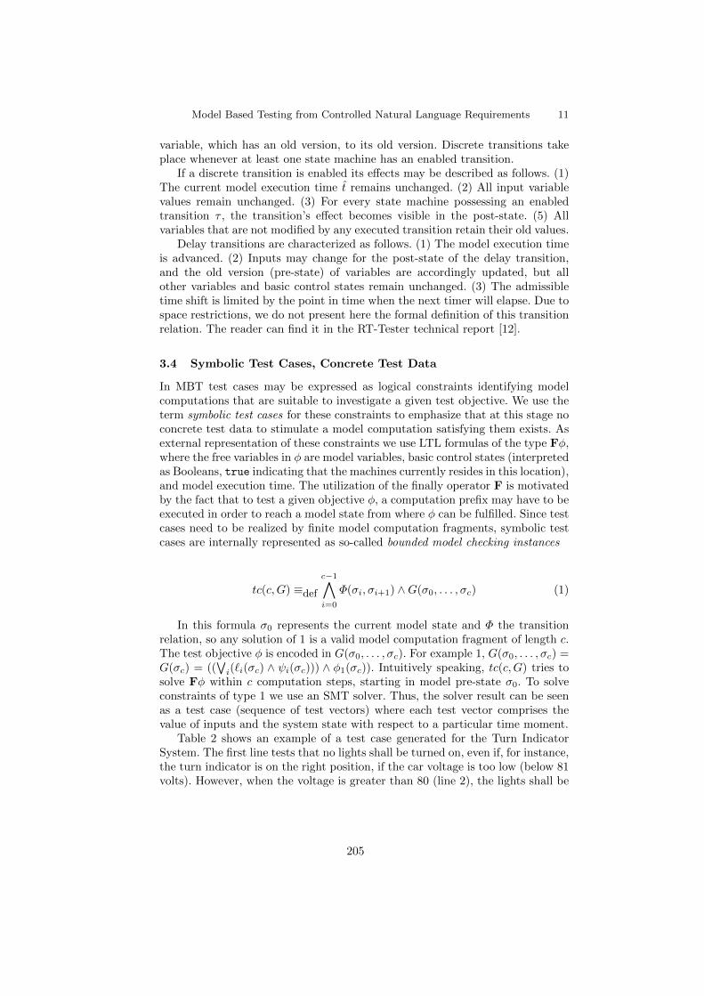
Model Based Testing from Controlled Natural Language Requirements 11

variable, which has an old version, to its old version. Discrete transitions takeplace whenever at least one state machine has an enabled transition.

If a discrete transition is enabled its effects may be described as follows. (1)The current model execution time t remains unchanged. (2) All input variablevalues remain unchanged. (3) For every state machine possessing an enabledtransition τ , the transition’s effect becomes visible in the post-state. (5) Allvariables that are not modified by any executed transition retain their old values.

Delay transitions are characterized as follows. (1) The model execution timeis advanced. (2) Inputs may change for the post-state of the delay transition,and the old version (pre-state) of variables are accordingly updated, but allother variables and basic control states remain unchanged. (3) The admissibletime shift is limited by the point in time when the next timer will elapse. Due tospace restrictions, we do not present here the formal definition of this transitionrelation. The reader can find it in the RT-Tester technical report [12].

3.4 Symbolic Test Cases, Concrete Test Data

In MBT test cases may be expressed as logical constraints identifying modelcomputations that are suitable to investigate a given test objective. We use theterm symbolic test cases for these constraints to emphasize that at this stage noconcrete test data to stimulate a model computation satisfying them exists. Asexternal representation of these constraints we use LTL formulas of the type Fφ,where the free variables in φ are model variables, basic control states (interpretedas Booleans, true indicating that the machines currently resides in this location),and model execution time. The utilization of the finally operator F is motivatedby the fact that to test a given objective φ, a computation prefix may have to beexecuted in order to reach a model state from where φ can be fulfilled. Since testcases need to be realized by finite model computation fragments, symbolic testcases are internally represented as so-called bounded model checking instances

tc(c,G) ≡def

c−1∧

i=0

Φ(σi, σi+1) ∧G(σ0, . . . , σc) (1)

In this formula σ0 represents the current model state and Φ the transitionrelation, so any solution of 1 is a valid model computation fragment of length c.The test objective φ is encoded in G(σ0, . . . , σc). For example 1, G(σ0, . . . , σc) =G(σc) = ((

∨i(`i(σc) ∧ ψi(σc))) ∧ φ1(σc)). Intuitively speaking, tc(c,G) tries to

solve Fφ within c computation steps, starting in model pre-state σ0. To solveconstraints of type 1 we use an SMT solver. Thus, the solver result can be seenas a test case (sequence of test vectors) where each test vector comprises thevalue of inputs and the system state with respect to a particular time moment.

Table 2 shows an example of a test case generated for the Turn IndicatorSystem. The first line tests that no lights shall be turned on, even if, for instance,the turn indicator is on the right position, if the car voltage is too low (below 81volts). However, when the voltage is greater than 80 (line 2), the lights shall be

205

12 G. Carvalho, F. Barros, F. Lapschies, U. Schulze, J. Peleska

turned on based on the turn indicator position (in this case, left position), andthe light shall remain on for 340ms, and off for 220ms, periodically.

Table 2. Example of Test Case.

TIME (ms) Voltage Emergency Button Turn Indicator Left Lights Right Lights0 80 off right off off

7918 81 off left on off8258 81 off left off off8478 81 off left on off

Note that symbolic test cases are not necessarily satisfiable, since some goalsG(σ0, . . . , σc) in the bounded model checking instance (1) may not admit a solu-tion, if they are generated by a purely syntactic evaluation of the IMR structure.

4 Tool Platform

The NAT2TESTIMR approach is fully supported by tools. The CNLParser isthe tool that receives the system requirements and, for each valid requirementwith respect to the SysReq-CNL, returns the corresponding ST. Next, the CF-Generator tool provides a semantic interpretation for each ST, using verb caseframes (CF) as semantic representation. After that, the tool IMR-Generatortranslates the case frames into the IMR.

Then, we use RT-Tester, a tool developed by Verified Systems InternationalGmbH in cooperation with the last author’s team at the University of Bremen,which operates on the IMR and outputs test cases with concrete test data. Op-tionally, the tool also generates the test procedures executing these test casesin software or system testing (hardware-in-the-loop) environments. To check theSUT responses against the test model (IMR), RT-Tester generates test oraclesfrom the given model. These run concurrently with the SUT, permanently check-ing SUT outputs against expected value changes and associated points in time.

5 Empirical Analyses

The NAT2TESTIMR approach was evaluated in four different examples. TheVending Machine (VM) example is an adaptation of the Coffee Machine pre-sented in [7]. The machine outputs weak coffee (within 10 and 30 seconds afterthe user request) if the user selects coffee too quickly (i. e., within 30 secondsafter inserting a coin), otherwise it outputs strong coffee. This example is aninteresting one since its behavior is highly dependent on time constraints. TheNuclear Power Plant Control (NPP) is a simplified version of a control systemfor safety injection in a nuclear power plant (NPP) as described in [8]. The Pri-ority Command Function (PC) was provided by Embraer. It comprises a systemthat decides whether the pilot or copilot will have priority in controlling theairplane side sticks based on their position and on a priority button. The Turn

206

Model Based Testing from Controlled Natural Language Requirements 13

Indicator System(TIS) is a simplification of the specification that is currentlyused by Daimler for automatically deriving test cases, concrete test data andtest procedures. In 2011, Daimler allowed the publication of this specification toserve as a “real-world” benchmark supporting research of MBT techniques. Oursimplification results in a size reduction of the original model presented in [11],but serves well as a proof of concept, because it still represents a safety-criticalsystem portion with real-time and concurrent aspects. Considering these exam-ples, we evaluated the NAT2TESTIMR approach from three perspectives: (i)performance; (ii) automatically generated versus manually written tests (onlyfor the Embraer example); and (iii) mutant-based strength analysis. All filesrelated to the empirical analyses (textual specification, case frames, IMR, testcases, and Java code) are publicly available7, except for the files related to theEmbraer example due to disclosure restrictions.

5.1 Results and Analyses

Table 3 summarizes the data collected. As it can be seen, the TIS is the largestexample: 1,124 words and 21 requirements, which comprises 600 thematic roles,whereas the other examples (VM, NPP, and PC) have an average of 320 words, 10requirements, and 182 thematic roles. As a consequence of its complexity, moresymbolic test cases are identified to the TIS example (193) when compared to theVM, NPP, and PC examples (62, 64, and 54 symbolic test cases, respectively).

The time measurements were done on an average configuration computer.The figures indicate that the time required to process (parse) the requirementsand identify the thematic roles is linear with respect to the specification size.Furthermore, these two tasks are performed in order of seconds. Differently, thetime required to generate the test cases from the obtained IMR had a sharperincrease with respect to the specification size. The most complex and largerspecification (TIS) required about 92 seconds, whereas the three other examplesneeded no more than a few seconds. Despite that, the total time required toapply the NAT2TESTIMR strategy is within 2 minutes in the worst case (TIS).As the RT-Tester infrastructure has already proven to scale up for the full TIS[11], we believe our strategy might scale as well since it reuses the RT-Testerinfrastructure and only adds a small overhead to process the requirements.

To evaluate the meaningfulness of the generated test vectors we compared thevectors generated by our approach with the ones manually written by Embraerspecialists. This analysis was not done for the other examples since we did nothave access to test vectors manually written for them. Our strategy generated 16of the 17 test vectors considered by the specialists (94.12%). The single missingvector exercises a system behavior that is already tested by other test vectors,and the strategies of the RT-Tester solver did not consider it. To evaluate thetest cases (sequence of test vectors) strength (ability to detect errors) we usemutation operators since it yields statistically trustworthy comparison of testcases strength in a controlled and systematic way [2]. Therefore, we created a

7 http://www.mbt-benchmarks.org

207

14 G. Carvalho, F. Barros, F. Lapschies, U. Schulze, J. Peleska

Table 3. Empirical Results of NAT2TESTIMR.

VM NPP PC TISGeneral Information

Words: 353 331 276 1,124Requirements: 11 11 8 21Thematic roles: 191 184 172 600Symbolic test cases: 62 64 54 193Covered symbolic test cases: 20 (32.26%) 48 (75.00%) 44 (81.48%) 121 (62.69%)

Time PerformanceTime to parse the requirements 0.59s 0.41s 0.03s 0.92sTime to identify thematic roles: 0.02s 0.03s 0.02s 0.05sTime to generate IMR and test cases: 1.07s 2.66s 0.95s 92.90sTotal time: 1.68s 3.10s 1.00s 93.87s

Vector Generation Precision AnalysisGenerated × manual vectors - - 16 (94.12%) -

Mutant-Based Strength AnalysisJava (LOC): 57 46 34 226Mutants generated: 364 317 144 1,126Mutation score: 54.67% 69.04% 87.50% 98.05%

“correct” (at least with respect to our tests) Java implementation (224 non-blank lines of code (LOC) in the largest case—TIS, and 34 LOC in the smallestcase—PC) for each example.

This implementation was created solely from the natural language require-ments, and we avoided any design decision that could not be inferred from therequirements. In other words, the abstract level of the Java specification is similarto the requirements one. Furthermore, it is important to note that the Java codewas created with the purpose of assessing our strategy, and in a real environmentthey would not be available yet, since we are generating test from initial andhigh-level requirements. We used the µJava tool [9] considering 12 method-levelmutation operators for generating mutants. This tool created between 144, and1,126 compiled mutants. Afterwards, we manually instrumented the Java code,and ran the test cases generated by the NAT2TESTIMR approach. From thesemutants, 54.67% were killed in the worst case (VM), whereas 98.05% were killedin the best case (TIS). It is worthy mentioning that the score obtained for thetest cases manually written by Embraer is 91.67%—near the NAT2TESTIMR

score (87.50%). We assumed a conservative approach [2] for analysis of largenumbers of mutants: we consider that all mutants are non-equivalent mutants.Therefore, these figures might be higher if equivalent mutants are identified anddiscarded.

The mutation score variation is justified by the number and percentage ofsymbolic test cases covered by the RT-Tester standard MC/DC coverage strat-egy, which was considered in all examples. As described in Section 3.4, sometimesonly a small number of the automatically generated symbolic test cases are satis-fiable, and thus a small number of test vectors are generated8. When it happens,in this case it is necessary to write user-defined test objectives to guide the testgeneration process, and thus generate more test vectors. As this approach is de-

8 In the tests described by Table 3, test data for all feasible symbolic test cases couldbe generated in an automated way.

208

Model Based Testing from Controlled Natural Language Requirements 15

pendent upon each example and user expertise, we did not consider it. As shownin Table 3, the lowest mutation score is related to the lowest number/coverageof symbolic test cases, and the symbolic test cases not covered are indeed notsatisfiable. Considering these results, the NAT2TESTIMR approach seems to bea reasonable alternative for generating test cases from CNL requirements. De-spite the promising results, some threats to validity might apply to our analyses.The main one concerns external validity: we considered few examples (small tomedium size), and thus we cannot generalize our results to other examples.

6 Related Work

Previous works [3, 16, 13] have already addressed the generation of tests fromNL specifications. Differently from this work, they do not impose a standard-ized way of writing as our SysReq-CNL does. Moreover, these works requireuser interaction during the process, whereas we do not. However, the strategyproposed in [13] is capable of generating tests for more concrete specifications(embedded with design decisions). We consider only high-level specifications. Theworks [4, 10, 15] provide a standardize way of writing requirements, but they donot deal with timed specifications and they generate non-executable test cases.However, the test generation of [10] is proved sound, whereas ours is not. Thework [14] considers time but within more limited requirement structures. In [5](NAT2TESTSCR) we use a transformation from CNL to the SCR notation in[5] and apply the T-VEC tool for generating tests. Differently, this paper uses anovel semantic encoding of the CNL behavior in the form of a timed transitionrelation. This new approach can handle time in a natural way, whereas in [5]auxiliary construction based on counters had to be applied.

7 Conclusion

This paper presented NAT2TESTIMR: an MBT technique based on natural lan-guage requirements. The requirements are syntactically analyzed according toour CNL, and their informal semantics is captured based on the Case Gram-mar theory. Then, the requirements semantics is automatically mapped into aTransition Relation, which provides the formal basis for MBT. Concrete testcases with associated data are generated with the support of an SMT solver.Our approach was evaluated considering four examples from different domains.Within seconds, it generated 94% of the test vectors manually written by spe-cialists. Moreover, considering a mutant-based strength analysis, our approachyielded a mutation score between 54% (worst case) and 98% (best case). Despitethe promising results, our approach is tailored for generating tests for high-levelrequirements of the form of action statements guarded by conditions, and thusother MBT techniques should be considered when testing more concrete speci-fications. Therefore, the tests generated by NAT2TESTIMR provide means forearly testing/simulation of models at design level. As future work we plan to(1) create a hierarchical IMR instead of our current flat structure, in order to

209

16 G. Carvalho, F. Barros, F. Lapschies, U. Schulze, J. Peleska

enhance the performance of our approach (we plan to consider the results of[6] for this purpose), and (2) extend of our approach for textual specification oftesting environments.

Acknowledgments. We thank Augusto Sampaio for his valuable advice. Thiswork has been partially funded by the EU FP7 COMPASS project (no.287829).

References

1. Allen, J.: Natural Language Understanding. Benjamin/Cummings (1995)2. Andrews, J.H., Briand, L.C., Labiche, Y.: Is mutation an appropriate tool for

testing experiments? In: International Conference on Software Engineering. pp.402–411. ACM, New York, NY, USA (2005)

3. Boddu, R., Guo, L., Mukhopadhyay, S., Cukic, B.: RETNA: from requirements totesting in a natural way. In: International Requirements Engineering (2004)

4. Brottier, E., Baudry, B., Traon, Y.L., Touzet, D., Nicolas, B.: Producing a globalrequirement model from multiple requirement specifications. In: International En-terprise Distributed Object Computing Conference. pp. 390–. USA (2007)

5. Carvalho, G., Falcao, D., Barros, F., Sampaio, A., Mota, A., Motta, L., Black-burn, M.: Test case generation from natural language requirements based on SCRspecifications. In: ACM Symposium on Applied Computing (2013)

6. Grieskamp, W., Gurevich, Y., Schulte, W., Veanes, M.: Generating finite statemachines from abstract state machines. Softw. Eng. Notes 27(4), 112–122 (2002)

7. Larsen, K., Mikucionis, M., Nielsen, B.: Online Testing of Real-time Systems usingUppaal: Status and Future Work. In: Dagstuhl Seminar Proceedings volume 04371:Perspectives of Model-Based Testing (2004)

8. Leonard, E.I., Heitmeyer, C.L.: Program synthesis from formal requirements spec-ifications using APTS. Higher Order Symbol. Comput. 16, 63–92 (March 2003)

9. Ma, Y.S., Offutt, J., Kwon, Y.R.: Mujava: an automated class mutation system:Research articles. Softw. Test. Verif. Reliab. 15(2), 97–133 (Jun 2005)

10. Nogueira, S., Sampaio, A., Mota, A.: Test generation from state based use casemodels. Formal Aspects of Computing 1, 1–50 (2012)

11. Peleska, J., Honisch, A., Lapschies, F., Loding, H., Schmid, H., Smuda, P., Vorobev,E., Zahlten, C.: A real-world benchmark model for testing concurrent real-time sys-tems in the automotive domain. In: Wolff, B., Zaidi, F. (eds.) Testing Software andSystems. Proceedings of the 23rd IFIP WG 6.1 International Conference, ICTSS2011. LNCS, vol. 7019, pp. 146–161. IFIP WG 6.1, Springer, Heidelberg (2011)

12. Peleska, J., Vorobev, E., Lapschies, F., Zahlten, C.: Automated model-based test-ing with RT-Tester. Tech. rep., Universitat Bremen (2011)

13. Santiago Jnior, V., Vijaykumar, N.L.: Generating model-based test cases fromnatural language requirements for space application software. Software QualityJournal 20, 77–143 (2012)

14. Schnelte, M.: Generating test cases for timed systems from controlled natural lan-guage specifications. In: International Conference on System Integration and Reli-ability Improvements. pp. 348–353 (2009)

15. Sinha, A., Jr., S.M.S., Paradkar, A.: Text2Test: Automated inspection of naturallanguage use cases. In: International Conference on Software Testing, Verificationand Validation. pp. 155–164. IEEE Computer Society, Washington (2010)

16. Sneed, H.: Testing against natural language requirements. In: International Con-ference on Quality Software. pp. 380 –387 (2007)

210

Refinement Tree and Its Patterns: a GraphicalApproach for Event-B Modeling

Kriangkrai Traichaiyaporn and Toshiaki Aoki

School of Information ScienceJapan Advanced Institute of Science and Technology (JAIST), Japan

{kriangkrai.tr, toshiaki}@jaist.ac.jp

Abstract. Event-B is a famous formal approach for verifying the re-quirements specification of safety-critical systems. Even though Event-Bis a good formal approach which is successful in applying to several prac-tical case studies, we think that additional methods are needed to apply itto the safety critical systems. Once we identify the requirements, Event-B allows us to formally describe the requirements. However, Event-Bdoes not explicitly support analysing and elaborating requirements them-selves. Although refinement mechanisms provided by Event-B is usefulto stepwise model concrete requirements from abstract ones, guideline ofthe refinements is not provided. This paper aims to propose a refinementtree diagram and its refinement patterns to provide the requirementsanalysis and elaboration, and the guideline for Event-B. The diagramand the patterns are partially derived from the KAOS method, a goal-oriented requirements engineering method. The utility of the diagramand the patterns is successfully shown by applying them to three prac-tical case studies.

1 Introduction

In the development of safety-critical systems, most of the typical approaches, toguarantee that the systems are sufficiently safe, start from ensuring the correct-ness of requirements specifications. Formal methods are recommended for ver-ifying the correctness by the functional safety standards such as ISO26262 [8].It is common that the requirements specifications are too complex to be for-mally verified all at once. Thus, refinement techniques are applied to reducedthe complexity by stepwise transforming an abstract specification into a con-crete specification. Among the refinement techniques, the refinement mechanismprovided by Event-B is a more flexible one comparing to the related languagessuch as Z [15] and VDM [9].

Event-B [3] is a formal specification language for modeling and verifyingsystem requirements through the refinement mechanism. Event-B has been suc-cessfully applied to several practical safety-critical systems. Some examples are atrain controller system [16], hybrid systems [17], and a metro system [14]. Event-B can be regarded as a method for correct-by-construction system development.

211

Even though Event-B is a good formal approach which is successful in apply-ing to several practical case studies, it lacks some methods, which are necessaryfor the practical development of the safety-critical systems. This paper focuseson dealing with two issues in Event-B. Firstly, Event-B provides no method foranalyzing and elaborating requirements specifications. The method is needed tospecify essential information of the safety-critical systems. Without sufficientlyspecifying the information, it is impossible to justify that a system is safe. Sec-ondly, there is no guideline for using the refinement mechanism in Event-B effec-tively. Given that a complicated system is being modeled in Event-B, designersand developers of the system might have no idea how to organize the refinementsteps which is a source of difficulty in the usage of refinement [2].

In this paper, we aim to fulfil what Event-B lacks by proposing a refinementtree diagram and its refinement patterns. The refinement tree diagram is tographically show the steps of refinement of the modeled specification in the formof tree structure. The diagram is designed in a way that it can be easily trans-formed into the Event-B specification. The refinement patterns are proposed inaddition to the diagram to guide the refinement of the Event-B specification.The diagram along with the patterns are created by adapting the concepts fromthe goal model and the goal refinement patterns of the KAOS method [19].

The KAOS method is a goal-oriented requirements engineering method foranalyzing and elaborating requirements. Its core model, the goal model, is cre-ated through the notion of goal refinement. The goal refinement provides a nearerway to how human stepwise refines requirements and is, thus, easy to understand.The KAOS method includes a set of goal refinement patterns to efficiently refinegoals by following the frequently-used refinement tactics. Seeing that the KAOSmethod provides what we need to fulfil Event-B, we apply the KAOS method toEvent-B. However, the formal semantics of the KAOS method and the formalspecification of Event-B are different. Their notions of refinement are differentas well. Consequently, instead of directly using the goal model, we propose therefinement tree diagram and the refinement patterns based on the goal modeland the goal refinement patterns.

The refinement tree diagram and the refinement patterns are applied to modelthree practical safety-critical case studies. From the case studies, we find thatwe can specify the necessary information, such as behavior, inputs, and output,through the refinement tree diagram in a similar manner to the KAOS method.Furthermore, the refinement patterns can guide the way to stepwise refine thespecifications of the case studies well. Therefore, we conclude that the refinementtree and the refinement patterns can complement Event-B.

The remainder of this paper is organized as follows. Section 2 overviewsEvent-B and the KAOS method. Section 3 explains the motivation behind thecreation of the refinement tree diagram. Section 4 and 5 describe the refinementtree diagram and its patterns respectively. Section 6 briefly demonstrates theapplication of our diagram and patterns on three case studies, and the results.Relevant issues from the results are discussed in Section 7. Related works arediscussed in Section 8. Finally, Section 9 concludes this paper.

212

2 Background

This section provides a short overview of Event-B and the KAOS method.

2.1 Event-B

Event-B [3] is a formal specification language for modeling specification of sys-tems. The language is based on first-order predicate logic and discrete transitionsystems. The main feature of Event-B is its refinement mechanism to incremen-tally constructing a specification from an abstract one into a concrete one.

A specification described in Event-B may be divided into a static part calledthe context, and a dynamic part called the machine. In this paper, we simplyassume that there is some context and do not mention it explicitly. Machines arefor describing behavioral properties of the specifications. Machines contain all ofthe state variables. Types and properties of the variables are declared throughinvariants in a form of the predicate. The values of the variables can be changedby the execution of events.

From an abstract machine containing a collection of variables, invariants, andevents, the refinement mechanism of Event-B allows us to refine the abstractmachine into a concrete machine by adding new variables, adding new events,rewriting events description to handle new variables, strengthening the guards,and so on. To explicitly associate the abstract machine and the concrete machine,a term ‘refines’ following with the name of the abstract machine is written in thedescription of the concrete machine. Even though there are many ways to refinea machine, they are restricted by the syntactic rules and the proof obligationsof Event-B. This is for preventing the description of the concrete machine fromcontradicting the description of the abstract machine.

Describing a specification in Event-B is always in a top-down style. TheEvent-B specification always start from describing the most abstract machinecalled ‘initial machine’. Then, the initial machine is gradually refined into thefirst refinement, the second refinement, and so on.

An event in a machine can be represented by the following form:

evt = refines a_evt anyp when G with W then S end

where a_evt is the name of the abstract event, p denotes internal parametersof the event, G is a predicate denoting guards, and S denotes the actions thatupdate some variables ands can be executed only when G holds. When we refinean abstract event, some variables of that event might be disappeared in itsconcrete event.W denotes witnesses that are additional elements in the concreteevent for indicating the disappeared variables and their values. Again, the term‘refines’ is written in the description of the concrete event to explicitly associateit with the corresponding abstract event. In the semantics of Event-B, if anevent does not have the term ‘refines’ in its description, it means that the eventimplicitly refine an event named skip, which is a blank event.

213

2.2 The KAOS method

KAOS (‘Knowledge Acquisition in autOmated Specification’ or ‘Keep All Ob-jects Satisfied’) [19] is a goal-oriented requirements engineering method withseveral UML-like models. The central model of the KAOS method is the goalmodel to show relationships among goals of a system in a tree structure.

The goal model consists of a refinement graph expressing how higher-levelgoals are refined into lower-level ones and, conversely, how lower-level goals con-tribute to higher-level goals. The higher-level goals are in general strategic andcoarse-grained whereas lower-level goals are technical and fine-grained. In a re-finement graph, a node represents a goal, and an AND-refinement link relatesa parent goal to a set of sub-goals. A parent goal must be satisfied when all ofits sub-goals are satisfied. The relationship between a parent goal and the set ofits sub-goals is called goal refinement. The process of goal refinement is intuitiveand can drive the analysis and elaboration of requirements. Formally, all goalscan be represented in linear temporal logic.

An effective way to construct a goal model is by reusing goal refinementpatterns [6]. The goal refinement patterns are frequently used patterns for re-fining a goal into sub-goals. Each pattern suggests specific refinements for in-stantiation to the specifics of the modeled system. For examples, the milestone-driven refinement pattern is for establishing a necessary intermediate step (amilestone condition) for reaching a target condition from a current condition,and the decomposition-by-case refinement pattern is to introduce different casesfor reaching a target condition. This pattern also checks that all possible casesare determined in the decomposition, and they are disjoint. The two examplesrefinement patterns are shown in Figure 1. Parameters are used in each patternfor representing conditions. Ones can instantiate a pattern by replacing each pa-rameter with a corresponding condition from the modeled system. The patternsare proved to be complete and consistent in term of the linear temporal logic.

Achieve[TargetCondition

If CurrentCondition]

Achieve[TargetCondition

If CurrentCondition]

Achieve[MilestoneCondition If CurrentCondition]

Achieve[MilestoneCondition If CurrentCondition]

Achieve[TargetCondition

If MilestoneCondition]

Achieve[TargetCondition

If MilestoneCondition]

(a) milestone-driven pattern

Achieve[TargetCondition]Achieve[TargetCondition]

Achieve[TargetCondition1

If Case1]

Achieve[TargetCondition1

If Case1]

Achieve[TargetCondition2

If Case2]

Achieve[TargetCondition2

If Case2]

If TargetCondition1or TargetCondition2

then TargetCondition

If TargetCondition1or TargetCondition2

then TargetCondition

Case1 XOR Case2Case1 XOR Case2

(b) decomposition-by-case pattern

Fig. 1. KAOS goal refinement patterns

In the context of the KAOS method, the pattern:

Achieve[TargetCondition (If CurrentCondition)]

214

prescribes goals where some target properties must be eventually satisfied in thefuture after a current condition is satisfied. The current condition can sometimesbe omitted in the pattern.

3 Motivation

The motivation behind this work comes from what we find in the existing worksapplying Event-B to practical case studies. An example is the work describingin [1], which is about the formalization of hybrid systems in Event-B. The hybridsystems are very important in the development of embedded systems where apiece of software, the controller, is supposed to manage an external situation,the environment. It is usual to find that most safety-critical systems are relatedto the hybrid systems. One hybrid system described in the article is about asystem controlling trains to provide safe moves of the trains. A preliminary studyis performed before the system is modeled in Event-B. From the preliminarystudy, some necessary invariants of the system are found, and the informationneeded for deciding the current acceleration of a train is specified. Withoutthe preliminary study, those necessary information cannot be specified. This canpotentially cause the system to be unsafe. The preliminary study is undoubtedlycrucial, but no systematical way for the preliminary study has been proposedfor Event-B.

Another notice from [1] is that even though the work focused on the hybridsystems, all of its examples have distinct ways to refine the system specificationsin Event-B. The advantage of the refinement mechanism is that it provide alot of (but limited) ways to refine an Event-B machine for widely supportingvarious kinds of systems. Unfortunately, the refinement mechanism is usuallypoorly used because it is not easy to decide how to organize the constructionsteps [2]. A guideline for the refinement is needed.

We find that the KAOS method provides the goal model to analyze andelaborate requirements through the intuitive notions of refinement, i.e. the goalrefinement. Besides, we think the requirements analysis and elaboration can beregarded as the preliminary study. Therefore, we plan to apply the goal modelto fulfil what Event-B lacks, that is, the systematical preliminary study and theguideline for using Event-B refinement.

Ideally, the most straightforward way to apply the goal model to Event-B isby using the goal model to model a system and then directly create an Event-Bspecification based on the goal model. However, the logic behind the two ap-proaches are different, i.e. the linear temporal logic and the first-order predicatelogic. In addition, their semantics of refinement are different. Goal refinementmeans that when all sub-goals are satisfied, then their parent goal is satisfied.The refinement mechanism is that a concrete machine preserves the propertiesdescribed in the abstract machine. Thus, it is difficult to directly apply the goalmodel to Event-B. As a result, we rather propose the refinement tree diagram toassist constructing and refining Event-B machines. The refinement tree diagramis similar to the goal model, but it can be transformed into Event-B specification.

215

Then, we propose a set of refinement patterns to help users to efficiently con-struct a refinement tree diagram similar to how the goal refinement patterns ofKAOS guide the construction of the goal model. Some of our refinement patternsare derived from the goal refinement patterns.

4 The Refinement Tree Diagram

Refinement tree diagram is a diagram showing refinements of event from a se-quence of refinements of Event-B machines in the form of tree. We design therefinement tree diagram in a way that it can graphically support:

– Demonstrating the refinements of events– Justifying new events and invariants of a machine– Separation of steps of refinement– Transformation to Event-B specification

Each node of the refinement tree diagram represents either an event or aninvariant. Arrows represent refinements of events and are used for separatingsteps of refinement. Lines among the nodes represent associations among thecomponents. An example of the refinement tree is shown in Figure 2. Throughthis example, all the details about the refinement tree diagram are graduallyexplained in the following subsections.

[Before >]

skip

Evt1When Q=TRUEThen R:=TRUE

Evt1When Q=TRUEThen R:=TRUE

Evt2When P=TRUEThen Q:=TRUE

Evt2When P=TRUEThen Q:=TRUE

Evt2When P=TRUEThen Q:=TRUE

Evt2When P=TRUEThen Q:=TRUE

Evt1_1When Q=TRUE and P=TRUEThen R=TRUE

Evt1_1When Q=TRUE and P=TRUEThen R=TRUE

Evt1_2When Q=TRUEThen R:=TRUE and P:=FALSE

Evt1_2When Q=TRUEThen R:=TRUE and P:=FALSE

If R=TRUE and P=FALSE then Q=TRUE

If R=TRUE and P=FALSE then Q=TRUE

Fig. 2. An example refinement tree diagram

4.1 Nodes

In the refinement tree diagram, a parallelogram represents an Event-B event,a trapezoid represents an Event-B invariant. Note that the description writtenin the parallelogram strictly follows the way the event is described in Event-Bspecification as explained in Section 2.1.

216

Each node representing either an event or an invariant is described by usingnatural language. The natural language acts as identifiers for formal descriptionsin Event-B . Even if it acts only as the identifiers, the meaning of the naturallanguage should correspond to the formal specification. Therefore, the naturallanguage that can be used in the diagram is limited to what the first-orderpredicate logic of Event-B can describe. For examples, if a predicate in Event-Bis written as (P = TRUE ∧ Q = TRUE) ⇒ R = FALSE where P , Q, R areBoolean variables, one possible identifier of this predicate in the natural languageis “If P and Q become true then R becomes false”. This is up to what P , Q, Rrepresent in the specification.

From Figure 2, the event skip acts as the root of the refinement tree diagramand it is always the root of all refinement tree diagrams. Excluding the root,the example has five events; Evt1, Evt2, Evt1_1, Evt1_2, and Evt2; and aninvariant. Note that there are two events written with the same descriptions.Both of them have the same name: Evt2.

4.2 Refinements of Events

A refinement of event is represented by an arrow with a small circle. The circle isfor linking all concrete events refining the same abstract event. Here, we specifythat ‘refinement of event’ means there are some changes in the description of aconcrete event comparing to its abstract event. If the description of a concreteevent is the same with its abstract event, we regard it as a ‘copy’ of the abstractevent. In this case, the arrow directly links two events to show the copy. Becauseabstract events belong to an abstract machine and concrete events belong to aconcrete machine, the arrow can separate level of the refinement tree diagram.

The level of the refinement tree diagram containing only the root is calledthe zeroth level. The zeroth level acts only as a root and is not necessary tobe transformed into Event-B specification. The subsequents levels are called thefirst level, the second level, and so on. They respectively correspond to the initialmachine, the first refinement, and so on in Event-B.

From Figure 2, the first level contains the events Evt1 and Evt2, where Evt1refines the root. The events of the first level must always refine the root, exceptthe event which can be linked with another event by some kinds of relationship.In the bottom level, Evt2 is a copy of Evt2 from the higher level, so theirdescriptions are the same. Evt1_1 and Evt1_2 refine Evt1. The bottom levelalso contains an invariant.

Both the refinement and the copy of event can be written into Event-B spec-ification as ‘refines’ relationships between abstract events and concrete events.Each event in an upper level must be pointed by at least one arrow from thesubsequent level, since Event-B does not allow any abstract events to be missingin the concrete machine.

217

4.3 Relationships among Events and Invariants

Here, we clearly separate the links showing relationships between events and thelinks showing relationships between events and invariants. They are representedby plain lines and dashed lines respectively. In facts, these relationships are notshown in the original Event-B. We define the relationships to support justifyingnew events and invariants of a machine in the refinement tree diagram. Theevents and invariants which are linked by the plain lines and the dashed linesmust be only in the same level of the refinement tree diagram.

In the context of this paper, ‘new’ events mean the events added to a concretemachine without explicitly refining an event from the abstract event. When thenew events are added to a machine, it might be unclear how the new eventsinteract with other events. The plain lines, linking two or more events, are definedfor the refinement tree diagram to show the interaction among new events andothers. The types of the relationship should also be written on the lines. Forexample, Evt2 and Evt1 in Figure 2 are linked by a ‘before’ relationship, whichmeans that Evt2 is necessary to be executed before Evt1. This is because theactions of Evt2 can trigger the guards of Evt1. Another type of relationshipused in this paper is the ‘parallel’ relationship. The events linked by the parallelrelationship means that they can interleave each other in the execution.

Invariants are needed for restricting possible values of variables. Thus, invari-ants also restrict the possible results of events. Conversely, events might provideus some ideas about important invariants needed to be include in a specification.These relationships between events and invariants can be shown in a refinementtree diagram through dashed lines between them as seen in Figure 2, whichcontains a link from an invariant to the event Evt1_2. For convention, if aninvariant is related to a set of concrete events which refines the same abstractevent, it should link with the small circle representing the refinement rather thanlinking with all the related events.

4.4 Transformation to Event-B specification

Since we allow using natural language to be identifiers of the Event-B descrip-tions for events and invariants and the descriptions always contain variables, sowe need to know all variables and data structure which can represent data andartifacts of a modeled system. In this paper, we assume that all needed variableshave been specified before creating a refinement tree diagram. Some approachesthat can be used for specifying the variables are the class diagram of KAOS [19]and the UML-B [13].

Regardless of how variables and data structures are specified, the transfor-mation from a refinement tree diagram into Event-B specifications can be donethrough the following principles:

– All events and invariants within the same level of a tree must be written inthe description of the same Event-B machine.

218

– Two consecutive levels of a refinement tree diagram means that the lowerlevel is a concrete machine refines the abstract machine from the upper level.This refinement relationship must be written in the concrete machine as theclause refines followed by the abstract machine’s name.

– An event in a refinement tree diagram contains the terms any, when, with,and then. Since these terms are directly derived from how an event is de-scribed in Event-B. Each term written in a parallelogram can directly mapto the corresponding terms of an event in Event-B.

– Each arrow from an abstract event to a concrete event can be representedin Event-B specification through the term refines followed by the name ofthe abstract event.

The example in Figure 2 can be easily transformed into two Event-B ma-chines. We assume that the variables P , Q, and R are Boolean variables. Thefollowings are parts of the machines which are derived from the example.

Initial machine:

Evt2 =when P = TRUEthen Q := TRUE end

Evt1 =when Q = TRUEthen R := TRUE end

First refinement:

Evt2 = refines Evt2

when P = TRUE then Q := TRUE end

Evt1_1 = refines Evt1

when Q = TRUE ∧ P = TRUE then R := TRUE end

Evt1_2 = refines Evt1

when Q = TRUE then R := TRUE ∧ P := FALSE end

Invariant :R = TRUE ∧ P = FALSE ⇒ Q = TRUE

5 The Refinement Patterns

An efficient way to create a goal model is by using the goal refinement pat-terns. We follow this concept by creating a set of refinement patterns for therefinement tree diagram. The refinement patterns are generic patterns to refinean abstract event into a set of concrete events with some invariants. Some re-finement patterns are derived from the frequent ways to refine a machine foundin the existing Event-B specifications created by others. Some refinement pat-terns are derived from the goal refinement patterns, since they are intuitiveand complete. At the moment, we have 4 patterns in total. Our original pat-terns are phase-decomposition refinement pattern and event-forking refinementpattern. The KAOS-based patterns are derived from the milestone-driven refine-ment pattern and the decomposition-by-case pattern as described in Section 2.2.The descriptions of each pattern can be found in the following subsections.

219

5.1 The phase-decomposition refinement pattern

...

skipskip

PHASE_1When guards of PHASE_1Then go to PHASE_2

PHASE_1When guards of PHASE_1Then go to PHASE_2

PHASE_2When guards of PHASE_2Then go to PHASE_3

PHASE_2When guards of PHASE_2Then go to PHASE_3

PHASE_NWhen guards of PHASE_NThen go to PHASE_1

PHASE_NWhen guards of PHASE_NThen go to PHASE_1

Fig. 3. The phase-decomposition-refinement pattern

The phase-decomposition refinement pattern (Figure 3) divides abstract be-havior of a system into two or more phases. One phase is represented by oneevent. Only the transition from one phase to another is described in each event.The flow of transitions is in the form of a cycle for iterative behavior of thesystem. This pattern is applicable for modeling an initial specification in Event-B. The possible phases used for dividing behavior of a system are: input phaseand decision phase. The input phase is for monitoring inputs of the system. Thedecision phase is for making a decision based on the inputs.

5.2 The event-forking refinement pattern

[parallel]Event_1When guardThen action_1

Event_1When guardThen action_1

Event_2When guardThen action_2

Event_2When guardThen action_2

Event_1_1When guardThen action_1_1

Event_1_1When guardThen action_1_1

Event_1_2When guardThen action_1_2

Event_1_2When guardThen action_1_2

Event_2_1When guardThen action_2_1

Event_2_1When guardThen action_2_1

Event_2_2When guardThen action_2_2

Event_2_2When guardThen action_2_2

Fig. 4. The event-forking refinement pattern

This pattern (Figure 4) is for describing environmental behavior which isusually non-deterministic and can behave in an arbitrary order. Inputs of asystem can be regarded as this kind of behavior. Thus, this pattern is applicableto describe the input phase of the system. We call the creation of a group ofarbitrarily ordering events as event forking. One event denotes one input. Theevent forking can be introduced to Event-B at both the higher level throughthe parallel relationship, and the lower level through the refinements withoutchanging the guards.

220

5.3 The milestone-driven refinement pattern

This pattern is for decomposing an abstract event into the sequences of two ormore concrete events. The decomposition is done by introducing intermediatesteps (milestones) between the guard and action of the abstract event. Figure 5shows the simplified form of the pattern, introducing just one intermediate stepto an abstract event. An invariants appearing in the pattern is to ensure thatafter one event is executed, its action can trigger the next event to form asequence of events.

5.4 The decomposition-by-case refinement pattern

This pattern is for refining an abstract into two or more concrete events fordealing with all possible cases of states of variables. One concrete event is sup-posed to deal with one case. This is to determine that which actions should beexecuted for each of the cases. Thus, this pattern is usually used in the decisionphase. It can also be used in the input phase, if there are some restrictions oninputs which needs to be determine case-by-case. An invariant included in thepattern is to ensure that all possible cases are determined, and they are disjoint.Figure 6 shows a simplified form of this pattern which contains only two cases.

[Before>]

EVTWhen guardThen action

EVTWhen guardThen action

EVT_MWhen guardThen action_M andsubphase_M:=TRUE

EVT_MWhen guardThen action_M andsubphase_M:=TRUE

EVTWhen guard_M and subphase_M=TRUEThen action

EVTWhen guard_M and subphase_M=TRUEThen action

If guard_M and subphase_M=TRUE

then guard

If guard_M and subphase_M=TRUE

then guard

Fig. 5. The milestone-driven refine-ment pattern

EventWhen guardThen action

EventWhen guardThen action

Event_C1When guard and case1Then action1

Event_C1When guard and case1Then action1

Event_C2When guard and case2Then action2

Event_C2When guard and case2Then action2

If guard then (case1 xor case2)

If guard then (case1 xor case2)

Fig. 6. The decomposition-by-case re-finement pattern

6 Case Studies

Since our objective of this research is about the practical usage of Event-B, weutilized our model in action on three examples derived from a real-world context.The examples can show the practical utility of the refinement tree diagram alongwith its patterns. The examples varied on their size and types of systems in orderto increase confidence in the utility of our approach.

Our approach was applied to a powered sliding door, an automatic gatecontroller, and Electrical Power Steering (EPS) system. The powered slidingdoor is derived from part 10 of ISO26262 [8]. The powered sliding door is a

221

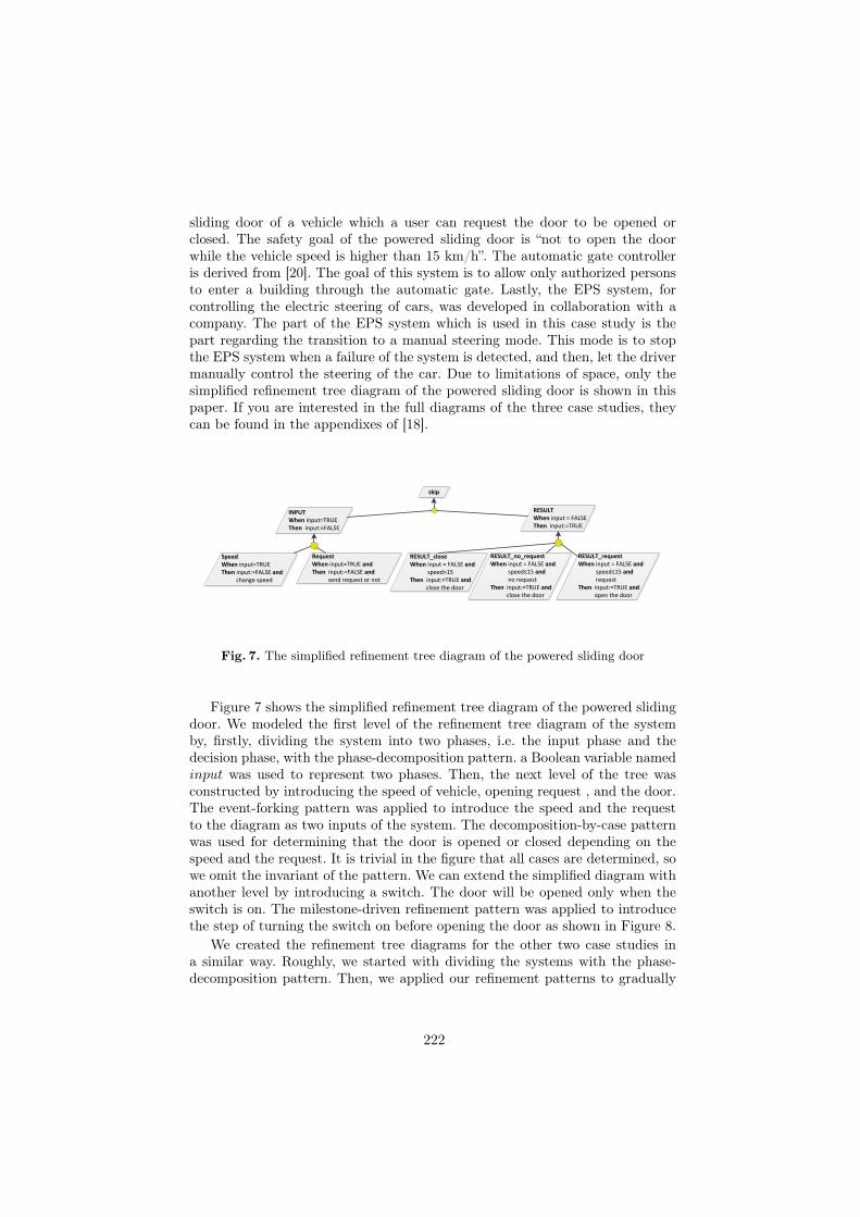
sliding door of a vehicle which a user can request the door to be opened orclosed. The safety goal of the powered sliding door is “not to open the doorwhile the vehicle speed is higher than 15 km/h”. The automatic gate controlleris derived from [20]. The goal of this system is to allow only authorized personsto enter a building through the automatic gate. Lastly, the EPS system, forcontrolling the electric steering of cars, was developed in collaboration with acompany. The part of the EPS system which is used in this case study is thepart regarding the transition to a manual steering mode. This mode is to stopthe EPS system when a failure of the system is detected, and then, let the drivermanually control the steering of the car. Due to limitations of space, only thesimplified refinement tree diagram of the powered sliding door is shown in thispaper. If you are interested in the full diagrams of the three case studies, theycan be found in the appendixes of [18].

skipskip

INPUTWhen input=TRUE Then input:=FALSE

INPUTWhen input=TRUE Then input:=FALSE

RESULTWhen input = FALSEThen input:=TRUE

RESULTWhen input = FALSEThen input:=TRUE

SpeedWhen input=TRUEThen input:=FALSE and change speed

SpeedWhen input=TRUEThen input:=FALSE and change speed

RequestWhen input=TRUE andThen input:=FALSE and send request or not

RequestWhen input=TRUE andThen input:=FALSE and send request or not

RESULT_closeWhen input = FALSE and speed>15Then input:=TRUE and close the door

RESULT_closeWhen input = FALSE and speed>15Then input:=TRUE and close the door

RESULT_no_requestWhen input = FALSE and speed≤15 and no requestThen input:=TRUE and close the door

RESULT_no_requestWhen input = FALSE and speed≤15 and no requestThen input:=TRUE and close the door

RESULT_requestWhen input = FALSE and speed≤15 and requestThen input:=TRUE and open the door

RESULT_requestWhen input = FALSE and speed≤15 and requestThen input:=TRUE and open the door

Fig. 7. The simplified refinement tree diagram of the powered sliding door

Figure 7 shows the simplified refinement tree diagram of the powered slidingdoor. We modeled the first level of the refinement tree diagram of the systemby, firstly, dividing the system into two phases, i.e. the input phase and thedecision phase, with the phase-decomposition pattern. a Boolean variable namedinput was used to represent two phases. Then, the next level of the tree wasconstructed by introducing the speed of vehicle, opening request , and the door.The event-forking pattern was applied to introduce the speed and the requestto the diagram as two inputs of the system. The decomposition-by-case patternwas used for determining that the door is opened or closed depending on thespeed and the request. It is trivial in the figure that all cases are determined, sowe omit the invariant of the pattern. We can extend the simplified diagram withanother level by introducing a switch. The door will be opened only when theswitch is on. The milestone-driven refinement pattern was applied to introducethe step of turning the switch on before opening the door as shown in Figure 8.

We created the refinement tree diagrams for the other two case studies ina similar way. Roughly, we started with dividing the systems with the phase-decomposition pattern. Then, we applied our refinement patterns to gradually

222

[Before>]

RESULT_requestRESULT_request

switch_onWhen input = FALSE and speed≤15 and requestThen speed_checked:=TRUE and switch is on

switch_onWhen input = FALSE and speed≤15 and requestThen speed_checked:=TRUE and switch is on

RESULT_requestWhen speed_checked=TRUE and switch is onThen input:=TRUE and door is opened and speed_checked=FALSE

RESULT_requestWhen speed_checked=TRUE and switch is onThen input:=TRUE and door is opened and speed_checked=FALSE

If speed_checked=TRUEand switch is on thenspeed≤15 and request

If speed_checked=TRUEand switch is on thenspeed≤15 and request

Fig. 8. Turning the switch on to open the door

introduce new inputs and concepts into subsequent levels of their trees. However,some nodes in some levels of their diagrams had to be determined manually. Mostof the manual events are the events which the variables in their descriptions arereplaced by new variables.

The full refinement tree diagrams of the powered sliding door, the automaticgate controller, and the EPS system have 4 levels, 5 levels, and 8 levels respec-tively. To discuss about the results, we counted the total number of events fromall levels of each resulted diagram. Those number are presented in Table 1. Here,we divided the events into two types according to their sources. ‘Manual’ meansthat the events are obtained manually, whereas ‘Patterns’ refers to the eventsthat are derived from the refinement patterns. Note that the number of thecopying events are omitted here. This is because the copying events are easilyderived and, thus, are irrelevant to the difficulty of the refinement.

Table 1. Number of events from the case studies according to sources of creation

Case study Manual Patterns TotalPowered Sliding Door 0 (0%) 19 (100%) 19

Automatic Gate Controller 8 (34.8%) 15 (65.2%) 23EPS System 18 (32.7%) 37 (67.3%) 55

7 Discussion

From Table 1, we found that, at least, around two-thirds of the events in theresulted refinement tree diagrams can be derived from our proposed refinementpatterns. The ‘Manual’ events were mostly for the replacement of variables withthe new ones. This kind of refinement can be regarded as vertical refinement forenriching the structure of a model to bring it closer to an implementation struc-ture [5]. Seeing that our approach focuses on specifying necessary information

223

for the safety requirements specification and the vertical refinement is just a sup-plement to the identified necessary information. Thus, it was acceptable that thepatterns cannot handle the vertical refinement at the moment. Therefore, we canconclude that the patterns are sufficient for modeling requirements specificationof the safety-critical systems. Besides, the applicability of the patterns did notdecrease when the specification was bigger. This fact can be discussed from thepercentage of the pattern-derived events of the automatic gate controller andthe EPS system that did not decrease much, even if the the EPS system was alot larger. As a result, the patterns are scalable.

In our experience modeling the case studies, we found that it was easy to jus-tify and structure Event-B specifications by using the refinement tree diagram.This was because the relationships among components of the specifications weregraphically shown. The concepts of the requirements analysis and elaborationand how to structurally stepwise refine the specifications were also provided bythe patterns, which were sufficient and scalable. We conclude that the refine-ment tree diagram and its patterns can fulfil what Event-B lacks as described inSection 3.

Since the mechanism of the goal refinement is designed for decomposing a goalinto two or more sub-goals, one-to-one refinement, i.e. a goal is decomposed intoa single sub-goal, rarely occurs in KAOS. However, the one-to-one refinementis possible in Event-B, e.g. we can just adding guards and/or actions into anevent for dealing with new variables of a concrete specification. Consequently, thenotations of the refinement tree diagram cannot handle the one-to-one refinementwell. This leads to the difficulty to create refinement patterns for the one-to-onerefinement in the form of the refinement tree. The incompetency to well handlethe one-to-one refinement is the current limitation of our approach. Actually,the vertical refinement are often the one-to-one refinement.

8 Related Work

There are many approaches aiming to use the capabilities of the KAOS methodto guide Event-B modeling. All of them focus on the direct application of thegoal model to Event-B, whereas our approach presents a new diagram basedon the goal model. The approach in [11] directly applied the goal refinementpatterns of KAOS to model a specification in Event-B. A way to describe andprove the KAOS goal refinement patterns in Event-B was defined. However, dueto the differences between KAOS and Event-B, it is not possible to representand prove all the goal refinement patterns in Event-B. This approach limits thecreation of a goal model to the application of only the compatible goal refinementpatterns. Rather, our approach provides a wider way to use patterns to guide therefinement by allowing the adaptation of the goal refinement patterns and thecreation of new patterns for Event-B itself. The approaches described in [4, 12]avoided the differences between the two frameworks by using only the leaf goalsof the goal model for modeling an initial specification in Event-B. This canbe done by regarding one leaf achieve goal as an event and/or an invariant.

224

Then, developers have to use other approaches to refine the initial specificationfurther. From this, the goal refinement does not relate to Event-B refinement.While, our approach uses the whole proposed diagram to model an initial Event-B specification along with the subsequent refinement steps.

We defined the refinement patterns of the refinement tree diagram for assist-ing the Event-B modeling. In [7], Hoang, Furst, and Abrial proposed that it ispossible to create design patterns for Event-B. They proved this fact by propos-ing provably-correct design pattern for a synchronous communication protocoland applied it to model another synchronous communication protocol. The pur-pose of the creation of their design patterns is to efficiently model a specificationin Event-B by reusing the existing Event-B specifications, which is similar toour purposes. Hence, this work supports the creation of our refinement patterns.Nonetheless, the refinements in their patterns are mostly the vertical refinementwhich are different from the refinements in our refinement patterns.

In 2012, Kobayashi and Honiden [10] proposed an approach to plan whatmodels are constructed in each abstraction level of Event-B. The advantage ofthis approach is that it can calculate how well a plan can mitigate the complexityof a specification. This calculation is useful for selecting a plan from a set ofplans. However, to make a set of plans, their approach needs that all details ofa system, such as behavior, are already identified before the calculation. Ourapproach lacks such calculation, but it is able to identify the necessary details,together with the guideline for Event-B refinement. Thus, their work and ourapproach can complement each other.

9 Conclusion

By observing the applications of Event-B in modeling specification of the safety-critical systems, we found that Event-B lacks the requirements analysis andelaboration, and the guideline for its refinement mechanism. To deal with theissues, we adapted the concepts of the goal model and the goal refinement pat-terns from the KAOS method to create the refinement tree diagram and therefinement patterns. The refinement tree diagram can graphically demonstratethe relationships among components of an Event-B specification. Thus, it is eas-ier to understand and justify the specification. The diagram was useful becauseit can be directly transformed into Event-B specifications. The refinement pat-terns were capable to guide how to stepwise refine Event-B specifications. Then,we successfully applied the refinement tree diagram and the patterns to threecase studies to model and verify them in Event-B. Therefore, the refinementtree diagram and the refinement patterns can complement Event-B. We believethat the approach described in this paper can encourage the use of the formalmethods like Event-B in the practical development of the safety-critical systems.

References

1. Jean-Raymond Abrial, Wen Su, and Huibiao Zhu. Formalizing hybrid systemswith Event-B. In Abstract State Machines, Alloy, B, VDM, and Z, pages 178–193.

225

Springer, 2012.2. J.R. Abrial. Formal methods in industry: achievements, problems, future. In

Proceedings of the 28th international conference on Software engineering, pages761–768. ACM, 2006.

3. J.R. Abrial. Modeling in Event-B: system and software engineering. CambridgeUniversity Press, 2010.

4. Benjamin Aziz, Alvaro Arenas, Juan Bicarregui, Christophe Ponsard, and PhilippeMassonet. From goal-oriented requirements to Event-B specifications. In FirstNasa formal method symposium (NFM 2009), Moffett Field, California , USA,April 2009.

5. Kriangsak Damchoom and Michael Butler. Applying event and machine decompo-sition to a flash-based filestore in Event-B. In Formal Methods: Foundations andApplications, pages 134–152. Springer, 2009.

6. Robert Darimont and Axel Van Lamsweerde. Formal refinement patterns for goal-driven requirements elaboration. ACM SIGSOFT Software Engineering Notes,21(6):179–190, 1996.

7. Thai Son Hoang, A Furst, and J-R Abrial. Event-B patterns and their tool support.In Software Engineering and Formal Methods, 2009 Seventh IEEE InternationalConference on, pages 210–219. IEEE, 2009.

8. CD ISO. 26262, road vehicles–functional safety, 2011.9. Cliff B Jones. Systematic software development using VDM, volume 2. Prentice

Hall Englewood Cliffs, 1990.10. T. Kobayashi and S. Honiden. Towards refinement strategy planning for Event-B.

arXiv preprint arXiv:1210.7036, 2012.11. Abderrahman Matoussi, Frédéríc Gervais, and Régine Laleau. A goal-based ap-

proach to guide the design of an abstract Event-B specification. In Engineering ofComplex Computer Systems (ICECCS), 2011 16th IEEE International Conferenceon, pages 139–148. IEEE, 2011.

12. Christophe Ponsard and Xavier Devroey. Generating high-level Event-B systemmodels from KAOS requirements models. In Actes du XXIIème Congrès INFOR-SID, pages 317–332, Lille, France, 2011.

13. Mar Yah Said, Michael Butler, and Colin Snook. Language and tool support forclass and state machine refinement in UML-B. In FM 2009: Formal Methods, pages579–595. Springer, 2009.

14. R. Silva. Lessons learned/sharing the experience of developing a metro system casestudy. arXiv preprint arXiv:1210.7030, 2012.

15. J Michael Spivey. The Z notation, volume 1992. Prentice Hall New York, 1989.16. W. Su, J.R. Abrial, R. Huang, and H. Zhu. From requirements to development:

methodology and example. Formal Methods and Software Engineering, pages 437–455, 2011.

17. W. Su, J.R. Abrial, and H. Zhu. Complementary methodologies for developinghybrid systems with Event-B. Formal Methods and Software Engineering, pages230–248, 2012.

18. Kriangkrai Traichaiyaporn. Modeling correct safety requirements using KAOS andEvent-B. Master’s thesis, School of Information Science, Japan Advanced Instituteof Science and Technology (JAIST), 2013. http://hdl.handle.net/10119/11496.

19. A. Van Lamsweerde. Requirements engineering: from system goals to UML modelsto software specifications, volume 3. Wiley, 2009.

20. D. Zowghi and V. Gervasi. On the interplay between consistency, completeness,and correctness in requirements evolution. Information and Software Technology,45(14):993–1009, 2003.

226

Formal Semantics and Analysis of Timed Rebecain Real-Time Maude

Zeynab Sabahi-Kaviani1, Ramtin Khosravi1, Marjan Sirjani2,1,Peter Csaba Olveczky3, and Ehsan Khamespanah1

1 School of Electrical and Computer Engineering, University of Tehran2 School of Computer Science, Reykjavik University

3 Department of Informatics, University of Oslo

Abstract. The actor model is one of the main models for distributedcomputation. Timed Rebeca is a timed extension of the actor-based mod-eling language Rebeca. Although Rebeca is supported by a rich verifica-tion toolset, Timed Rebeca has not had an executable formal semantics,and has therefore had limited support for formal analysis. In this paper,we provide a formal semantics of Timed Rebeca in Real-Time Maude.We have automated the translation from Timed Rebeca to Real-TimeMaude, allowing Timed Rebeca models to be automatically analyzed us-ing Real-Time Maude’s reachability analysis tool and timed CTL modelchecker. This enables a formal model-based methodology which combinesthe convenience of intuitive modeling in Timed Rebeca with formal ver-ification in Real-Time Maude. We illustrate this methodology with acollision avoidance protocol for wireless networks.

1 Introduction

The importance of formal modeling and analysis for ensuring the dependabilityand correctness of safety-critical systems has long been acknowledged. How-ever, the lack of formal modeling languages close to programming and modelinglanguages used by practitioners has limited the use of formal methods. TimedRebeca [1] is an actor-based [2] modeling language that extends the Rebeca lan-guage [17] to support the modeling of distributed real-time systems. Becauseof its Java-like syntax and its simple and intuitive message-driven and object-based computational model, Timed Rebeca is an easy-to-learn language for sys-tem developers, thereby bridging the gap between formal methods and practicalsoftware engineering.

Although Rebeca is supported by a rich model checking toolset [15], modelchecking of Timed Rebeca models has not been supported until now. Eventhough Timed Rebeca has an SOS semantics, it lacks an executable formal se-mantics that would enable automated analysis methods such as simulation andtemporal logic model checking.

However, providing an executable formal semantics for Timed Rebeca is quitechallenging. For example, since Timed Rebeca has a rich expression/statementlanguage that allows the values of state variables to grow beyond any bound,

227

and since the message queues can become arbitrarily long, Timed Rebeca cannotbe translated into popular real-time formalisms such as, e.g., timed automata.

In this paper, we provide a formal Real-Time Maude semantics for TimedRebeca. Real-Time Maude [12] is a specification formalism and analysis tool forreal-time systems based on rewriting logic [11]. With its natural time model andexpressive formalism, which is particularly suitable for formally specifying dis-tributed real-time systems in an object-oriented way, Real-Time Maude shouldbe ideally suited for this challenging task. Real-Time Maude is supported by ahigh-performance toolset providing a spectrum of analysis methods, includingsimulation through timed rewriting, reachability analysis, and (untimed) lineartemporal logic model checking as well as timed CTL model checking.

We have automated the translation from Timed Rebeca to Real-Time Maude,so that the user gets Real-Time Maude simulation and model checking of his/herTimed Rebeca model for free. Furthermore, such formal analysis is being inte-grated into the Rebeca toolset. This would of course not be very useful if theuser would need to understand the Real-Time Maude representation of his/herTimed Rebeca model, and/or would need to define state properties in Real-TimeMaude, in order to model check his/her Timed Rebeca model. We have thereforetaken advantage of Real-Time Maude’s support for parametric state propositionsto predefine useful generic state propositions, so that the user can define his/her(possibly timed) temporal logic properties without having to know Real-TimeMaude or understand how the mapping from Timed Rebeca works.

Altogether, this enables a formal model-engineering methodology that com-bines the convenience of modeling in an intuitive actor language with Java-likesyntax with formal verification in Real-Time Maude. We illustrate this method-ology with a collision avoidance protocol case study.

The rest of the paper is structured as follows. Section 2 briefly introducesTimed Rebeca and Real-Time Maude. Section 3 explains the Real-Time Maudeformalization of the Timed Rebeca semantics. Section 4 defines some usefulgeneric atomic state propositions that allows the user to easily define his/hertemporal logic formulas without knowing Real-Time Maude. Section 5 illustratesour methodology on a collision avoidance protocol. Finally, Section 6 discussesrelated work and Section 7 gives some concluding remarks.

2 Preliminaries

2.1 Timed Rebeca

Since Timed Rebeca is an extension of the Rebeca modeling language, we firstintroduce Rebeca and then explain Timed Rebeca in more detail.

Rebeca [17] is a pure actor-based modeling language suitable for specifyingdistributed systems. Rebeca is supported by a rich model checking toolset [15].

A Rebeca model consists of a set of actors (called rebecs) that communicateasynchronously by message passing. Each actor maintains a queue of messagesthat it has received but not yet processed. An actor repeatedly takes a message

228

Model ::= Class∗ Main

Main ::= main { InstanceDcl∗ }InstanceDcl ::= className rebecName(〈rebecName〉∗) : (〈literal〉∗);

Class ::= reactiveclass className { KnownRebecs Vars Constr MsgSrv∗ }KnownRebecs ::= knownrebecs { VarDcl∗ }

Vars ::= statevars { VarDcl∗ }VarDcl ::= type 〈v〉+;

Constr ::= className methodName(〈type v〉∗) { Stmt∗ }MsgSrv ::= msgsrv methodName(〈type v〉∗) { Stmt∗ }

Stmt ::= v = e; | v =?(e1, . . . , en) | Send ; | if (e) { Stmt∗ } [else { Stmt∗ }] |delay(e); | for (Stmt1; e; Stmt2) { Stmt∗ }

Send ::= rebecName.methodName(〈e〉∗) [after(e)] [deadline(e)]

Fig. 1. Abstract syntax of Timed Rebeca. Angle brackets 〈...〉 are used as meta paren-thesis. Identifiers className, rebecName, methodName, v, literal , and type denote classname, rebec name, method name, variable, literal, and type, respectively; and e de-notes an (arithmetic or boolean) expression. In for loops, Stmt1 is the initializationstatement, e2 is a boolean expression (the loop execution condition), and Stmt2 is theupdate statement (executed after each iteration).

from the beginning of its queue and executes the corresponding message server,which may involve sending messages to other actors and changing the actor’s lo-cal state. Execution is non-preemptive: the actor does not take the next messagefrom its queue before the running message server is finished.

A Rebeca specification defines a number of reactive classes and a main block.A reactive class defines an actor type and its behavior as well as its relationshipto other actors. The body of a reactive class definition has three sections: knownrebecs, state variables, and message servers. A rebec can only send messages toits known rebecs. The local state of a rebec is given by the values of its statevariables. The type of state variables can be integer types, Boolean, and arrays.

The message servers specify how the rebecs respond to incoming messages.They may have parameters and may define local variables. The body of a messageserver consists of a number of statements, including assignments, conditionals,loops, and sending messages. The expressions contains common arithmetic andlogical operators. The nondeterministic assignment v =?(e1, . . . , ek) nondeter-ministically assigns (the current evaluation of) one of the expressions ei to thevariable v. Each class has a constructor (with the same name as the class) whichinitializes the state variables of its instances.

Timed Rebeca [1] is a timed extension of Rebeca whose abstract syntax isgiven in Fig. 1. The following timed features have been added for specifyingdistributed real-time systems:

229

– delay is a statement used to model computation times. Since we assume thatthe execution times of the other statements to be zero, the computation timemust be specified by the modeler using the delay statement.

– after is a time tag attached to a message and defines the earliest time themessage can be served, relative to the time when the message was sent.

– deadline is a time tag attached to a message which determines the expirationtime of the messages, relative to the time when the message was sent.

When a message with tag after t is sent, it is added to the set of undeliveredmessages and resides there until t time units have elapsed. Then, it is delivered,i.e., appended to the receiving rebec’s message queue. The messages in a rebec’squeue are therefore ordered according to their delivery time (if the deliverytime of two messages are the same, the order in which they are delivered isselected nondeterministically). If the deadline of a message is reached, regardlessof whether it is delivered or not, the message is purged. A rebec takes a messagefrom its queue as soon as it can (i.e., when it has finished processing the previousmessage, and there are some messages in the queue).

Figure 2 shows a Timed Rebeca model of a simple thermostat system com-posed of two actors t and h of reactive classes Thermostat and Heater, respec-tively. The actors are instantiated in the main block; e.g., Heater h(t):();

creates an instance h of Heater, passing t as its known rebec, and invokingits constructor (with empty parameter list). The goal of the system is to keepthe temperature between 25 and 30 degrees. The Thermostat actor checks thetemperature every 5 time units, by sending a checkTemp message to itself (line19). If the temperature is not in the acceptable range, it sends the Heater actorh the proper on or off message, which expires after 20 time units (lines 16 and18). It takes two time units for the heater to turn itself on or off. The heateralso models the change in the environment by nondeterministically changing thetemperature by 1 to 3 degrees every 10 time units (lines 47-49), and sending thedelta to the heater (line 50).

2.2 Real-Time Maude

Real-Time Maude [13, 12] extends the rewriting-logic-based Maude language andtool [5] to support the formal specification and analysis of real-time systems. AReal-Time Maude timed module is a tuple (Σ,E,IR,TR), where:

− (Σ,E) is a membership equational logic [5] theory where Σ is an algebraicsignature, declaring the sorts, subsorts, and functions of the system, and Ea set of confluent and terminating conditional equations. (Σ,E) specifies thesystem’s states as an algebraic data type, and must contain a specificationof a sort Time modeling the (discrete or dense) time domain.

− IR is a set of (possibly conditional) labeled instantaneous rewrite rules spec-ifying the system’s instantaneous (i.e, zero-time) local transitions, writtenwith syntax rl [l] : u => v, where l is a label. Such a rule specifies a one-step transition from an instance of the term u to the corresponding instanceof the term v. The rules are applied modulo the equations E.

230

1 reactiveclass Thermostat {

2 knownrebecs {

3 Heater heater;

4 }

5 statevars {

6 int period;

7 int temp;

8 }

9 Thermostat() {

10 period = 5;

11 temp = 25;

12 self.checkTemp();

13 }

14 msgsrv checkTemp() {

15 if (temp >= 30)

16 heater.off() deadline(20);

17 if (temp <= 25)

18 heater.on() deadline(20);

19 self.checkTemp()

after(period);

20 }

21 msgsrv changeTemp(int delta) {

22 temp = temp + delta;

23 }

24 }

26 reactiveclass Heater {

27 knownrebecs {

28 Thermostat thermostat;

29 }

30 statevars {

31 boolean on;

32 int delta;

33 }

34 Heater() {

35 on = false;

36 self.run();

37 }

38 msgsrv on() {

39 delay(2);

40 on = true;

41 }

42 msgsrv off() {

43 delay(2);

44 on = false;

45 }

46 msgsrv run(){

47 delta = ?(1,2,3);

48 if (on == false)

49 delta = -1 * delta;

50 thermostat.changeTemp(delta);

51 self.run() after(10);

52 }

53 }

55 main {

56 Thermostat t(h):();

57 Heater h(t):();

58 }

Fig. 2. The Timed Rebeca model for a simple thermostat/heater system.

− TR is a set of (usually conditional) tick rules, written with syntax crl [l] :

{t} => {t′} in Time τ if cond, that model time elapse. { } is a built-inconstructor of sort GlobalSystem, and τ is a term of sort Time that denotesthe duration of the rewrite.

The initial state must be a ground term of sort GlobalSystem and must bereducible to a term of the form {u} using the equations in the specification.

The Real-Time Maude syntax is fairly intuitive. A function symbol f in Σis declared with the syntax op f : s1 ... sn -> s, where s1...sn are the sortsof its arguments, and s is its result sort. Equations are written with syntaxeq u = v, and ceq u = v if cond for conditional equations. The mathemati-cal variables in such statements are declared with the keywords var and vars.An equation f(ti, . . . , tn) = t with the owise (for “otherwise”) attribute canbe applied to a subterm f(. . .) only if no other equation with left-hand sidef(u1, . . . , un) can be applied.

A class declaration class C | att1 : s1, ... , attn : sn declares aclass C with attributes att1 to attn of sorts s1 to sn, respectively. An objectof class C is represented as a term < O : C | att1 : val1 ,..., attn : valn >

231

where O, of sort Oid is the object’s identifier, and where val1 to valn arethe current values of the attributes att1 to attn. The state is a term of sortConfiguration, and has the structure of a multiset of objects and messages,with multiset union denoted by a juxtaposition operator that is declared asso-ciative and commutative, so that rewriting is multiset rewriting.

The dynamic behavior of concurrent object systems is axiomatized by spec-ifying each of its transition patterns by a rewrite rule. For example, the rule

rl [l] :

m(O,W)

< O : C | a1 : X, a2 : O’, a3 : Z >

=>

< O : C | a1 : X + W, a2 : O’, a3 : Z >

dly(m’(O’),X) .

defines a parameterized family of transitions in which a message m, with param-eters O and W, is read and consumed by an object O of class C. The transitionschange the attribute a1 of the object O and send a new message m’(O’) withdelay X.

Formal Analysis. The Real-Time Maude tool provides a spectrum of analysismethods, including:

– timed rewriting that simulates one behavior of the system up to certainduration from an initial state;

– timed search analyzes whether a state matching a state pattern is reachablefrom the initial state within a certain time interval;

– model checking to check whether each possible behavior from the initial statesatisfies a temporal logic formula. Real-Time Maude extends Maude’s lin-ear temporal logic model checker. State proposition are terms of sort Prop,and their semantics should be given by (possibly conditional) equations ofthe form {statePattern} |= prop = b, for a b a term of sort Bool, whichdefines the state proposition prop to hold in a state {t} if {t} |= prop evalu-ates to true. A temporal logic formula is constructed by state propositionsand temporal logic operators such as True, False, ∼ (negation), /\, \/, ->(implication), [] (“always”), <> (“eventually”), and U (“until”). The time-bounded model checking command has the syntax mc {t} |=t ϕ in time

<= τ . for initial state {t} and temporal logic formula ϕ. Real-Time Maudehas also recently been equipped with a model checker for timed computationtree logic (TCTL) properties [10].

3 Real-Time Maude Semantics of Timed Rebeca

This section explains how we have formalized the semantics of Timed Rebeca inReal-Time Maude in an object-oriented style.

232

Specifying the Static Parts. In the Real-Time Maude semantics of a TimedRebeca model we need to keep track of (i) the declarations of the (messageservers of the) reactive classes; (ii) the rebecs in their current states; and (iii)the set of as-yet undelivered messages.

Since the message servers do not change dynamically, we do not need to carrythem around in the state. Instead, the message servers are modeled by a function

op msgServer : ClassName MsgHeader -> Statements .

where msgServer(c, m) defines the code to be executed by a rebec of reactiveclass c when it treats a message with header m. The sort Statements is astraight-forward representation of the body of a message server. For example, inour thermostat example, msgServer(Thermostat, Thermostat) equals

(period := 5) ; (temp := 25) ;

(sendSelf checkTemp with noArg deadline INF after 0)

and msgServer(Thermostat, checkTemp) equals

(if( temp >= 30 ) then (send off with noArg to "heater" deadline 20 after 0)) ;

(if( temp <= 25 ) then (send on with noArg to "heater" deadline 20 after 0)) ;

(sendSelf checkTemp with noArg deadline INF after 5)

We also have a function formalParams such that formalParams(c, m) returnsthe list of the formal parameters of the message server for m in reactive class c.

We mostly omit the details of how basic Rebeca statements (e.g., assignmentsand evaluation of expressions) are formalized in Real-Time Maude, and referto [3] for a thorough treatment of the Real-Time Maude formalization of theevaluation of expressions in a fairly sophisticated language. The only expressionwe mention is due to the possibility of having nondeterministic assignments. Weformalize the expression list ? (e1, e2, . . . , en) in a nondeterministic assignmentas a list e1 ? e2 ? . . . ? en using the following list data type:

sort NDExpr . subsort Expr < NDExpr .

op nil : -> NDExpr .

op _?_ : NDExpr NDExpr -> NDExpr [assoc id: nil] .

Since nil is the identity element for lists, Maude considers l and nil ? l andl ? nil to be identical lists. In particular, a single expression e is considered byMaude to be identical to the lists nil ? e and e ? nil and nil ? e ? nil.

The state of the Real-Time Maude representation of a Timed Rebeca modelis a multiset consisting of one Rebec object for each rebec in the system and onemessage for each message in the set of undelivered messages.

A rebec is modeled by an object instance of the following class Rebec:

class Rebec | stateVars : Valuation, queue : MsgList,

classId : ClassName, toExecute : Statements,

knownRebecs : KnownList .

where stateVars represents the state variables of the rebec and the formal pa-rameters of the message server being treated, together with their current values,as a set of terms of the form var-name |-> value; queue is a ‘::’-separated list

233

of messages representing the message queue of the rebec; classId is the nameof the reactive class of the rebec; toExecute denotes the remaining statementsthe rebec has to execute (and is noStatements if the rebec is not executing amessage server); and knownRebecs denotes the “known rebecs” of the rebec.

For example, the following term models the rebec "t" of class Thermostat

right after completing its constructor. Its state variables have the values 5 and25, there is only one message in its queue (sent by itself), and the rebec is notexecuting any message server.

< "t" : Rebec | stateVars : (’period |-> 5) (’temp |-> 25),

queue : (checkTemp with noArg from "t" to "t" deadline INF),

classId : Thermostat,

toExecute : noStatements,

knownRebecs : (Heater heater --> "h") >

Communication between rebecs takes place when a rebec sends a messageto another rebec (or to itself). The message is put into the multiset of undeliv-ered messages until its message delay ends. It is then delivered to the receiver’smessage queue. Delivered messages are modeled using the constructor

msg _with_from_to_deadline_ : MsgHeader Valuation Oid Oid TimeInf -> Msg .

A delivered message therefore contains a header (the message name), its argu-ments, the id of the sender rebec, the id of the receiver, and the time remaininguntil the expiration (deadline) of the message. Delayed messages have the formdly(m, t), where m is a message as above and t is the remaining delay of themessage, and where dly(m, 0) is considered to be identical to m [12].

Instantaneous Transitions. We next formalize the instantaneous actions of aTimed Rebeca rebec using rewrite rules. We show 9 of the 16 rewrite rules thatdefine our semantics of the Timed Rebeca.

In the following rule, an idle rebec takes the first message from its queue andstarts executing the statements in the corresponding message server by puttingthose statements into its toExecute attribute. Some additional bookkeeping isalso required: the formal parameters of the message server must be initialized tothe values in the message and added to the state variables; to clean up at theend of the execution, we add a new statement removeVars to execute after thestatements in the message server have been executed:4

rl [takeMessage] :

< O : Rebec | stateVars : SVARS,

queue : (M with VAL from O’ deadline DL) :: MSGLIST,

classId : C, toExecute : noStatements >

=>

< O : Rebec | stateVars : SVARS VAL (’sender |-> O’),

queue : MSGLIST,

toExecute : msgServer(C, M) ; removeVars(VAL (’sender |-> O’)) > .

4 In this paper we follow the Maude convention that variables are written with (only)capital letters, and do not show the variable declarations.

234

Because of the possibility of having nondeterministic assignments, the rewriterule modeling (both deterministic and nondeterministic) assignment is interest-ing. The following rule uses pattern matching and the fact that the list con-catenation operator ? is declared to be associate and to have identity nil tonondeterministically select any possibly expression EX from a list of expressions.This rule also covers deterministic assignment, since the list variables LIST1 andLIST2 may both match the empty list nil. In addition, the rebec updates itstoExecute attribute to only execute the remaining statements:

rl [detAndNondetAssignment] :

< O : Rebec | stateVars : (VAR |-> VAL) SVARS,

toExecute : (VAR := LIST1 ? EX ? LIST2) ; STMTLIST >

=>

< O : Rebec | stateVars : (VAR |-> evalExp(EX, (VAR |-> VAL) SVARS)) SVARS,

toExecute : STMTLIST > .

We next describe the semantics of loops for (init; cond; update){body},where init is a statement executed once in the beginning, cond is a Booleanexpression that must be true to continue the iterations, update is a statementexecuted after each iteration, and body is a statement list executed in each iter-ation. The semantics of loops is formalized in a standard “unfolding” style:

rl [forLoop] :

< O : Rebec | toExecute : for(INIT, COND, UPDATE, BODY) ; STMTLIST >

=>

< O : Rebec | toExecute : INIT ; iterate(COND, UPDATE, BODY) ; STMTLIST > .

rl [iterate] :

< O : Rebec | stateVars : SVARS,

toExecute : iterate(COND, UPDATE, BODY) ; STMTLIST >

=>

< O : Rebec | toExecute : if evalBoolExp(COND, SVARS) then

BODY ; UPDATE ; iterate(COND, UPDATE, BODY) ; STMTLIST

else STMTLIST fi > .

If the first statement is a send statement, the rebec creates a delayed messagewhich is added to the undelivered message soup.

rl [sendMessage] :

< O : Rebec | stateVars : SVARS,

toExecute : (send M with ARGS to REC deadline DL after AFT)

; STMTLIST , knownRebecs : (CN NK --> RCVR) NL >

=>

< O : Rebec | toExecute : STMTLIST >

dly(M with getVals(ARGS, SVARS, formalParams(CN,M)) from O to RCVR

deadline evalIntExp(DL,SVARS),

evalIntExp(AFT,SVARS)) .

Both DL and AFT are expressions evaluated using evalIntExp in the contextof the current variable assignment SVARS. The created message is added to thesystem configuration; when its remaining delay becomes 0, the message becomes“undelayed” as explained above, and can be received by the intended recipient,which puts the message into its message queue:

235

rl [readMessage] :

(M with ARGS from O to O’ deadline DL )

< O’ : Rebec | queue : MSGLIST >

=>

< O’ : Rebec | queue : MSGLIST :: (M with ARGS from O deadline DL) > .

Another interesting case is the execution of a delay statement, which istreated as follows: When the rebec encounters the delay statement, it evalu-ates the delay expression using the current values of the variables. Once it hasdone that, it leaves the delay statement in the beginning of its toExecute at-tribute until the remaining delay becomes 0, when the rebec just continues withthe next statement. Decreasing the remaining delay is done by the tick rule be-low. The following rules then, respectively, evaluate the delay expression at thebeginning of the delay, and finish the delay when the remaining delay is 0:

crl [evaluateDelayExpression] :

< O : Rebec | stateVars : SVARS, toExecute : delay(EX) ; STMTLIST >

=>

< O : Rebec | toExecute : delay(evalIntExp(EX, SVARS)) ; STMTLIST >

if not (EX :: Int) .

rl [endDelay] :

< O : Rebec | toExecute : delay(0) ; STMTLIST >

=>

< O : Rebec | toExecute : STMTLIST > .

Timed Behavior. The following “standard” object-oriented tick rule [12] isused to model time advance until the next time when something must “happen”:

var SYSTEM : Configuration .

crl [tick] : {SYSTEM} => {elapsedTime(SYSTEM, mte(SYSTEM))} in time mte(SYSTEM)

if mte(SYSTEM) > 0 .

The variable SYSTEM matches the entire state of the system. The function mte

(maximal t ime elapse) determines how much time can advance in a given state.If an instantaneous rule is enabled, it must be executed immediately; therefore,mte of a state must be zero when an instantaneous rule is enabled in that state.

The function mte is the minimum of the mte of each rebec and each messagein the soup. As mentioned above, the mte must be 0 when the rebec has astatement to execute which does not have the form delay(i), for an integer i;in the latter case, the mte equals i. If there are no statements to be executed,the mte equals 0 if the rebec has a message in its queue, and equals the infinityvalue INF if the message queue is empty:

op mte : Configuration -> TimeInf [frozen (1)] .

eq mte(none) = INF .

eq mte(dly(M, T) CONF) = min(T, mte(CONF)) .

ceq mte(OBJECT CONF) = min(mte(OBJECT), mte(CONF)) if CONF =/= none .

eq mte(< O : Rebec | toExecute : noStatements, queue : empty >) = INF .

eq mte(< O : Rebec | toExecute : delay(T) ; STMTLIST >) = T .

eq mte(< O : Rebec | >) = 0 [owise] .

236

The function elapsedTime models the effect of time elapse on a state asfollows: The effect of time elapse on a rebec is that the remaining time until themessage deadline is decreased according to the elapsed time for each messagein the queue. Furthermore, the remaining delay of a delay statement being ex-ecuted is also decreased according to the elapsed time. For messages travelingbetween rebecs, their remaining delays and deadline are decreased according tothe elapsed time. In both cases, if the deadline expires before the message istreated, the message is purged (i.e., becomes the empty configuration none):

op elapsedTime : Configuration Time -> Configuration [frozen (1)] .

eq elapsedTime(none, T) = none .

eq elapsedTime(dly(M with ARGS from O to O’ deadline T1, T2) CONF, T)

= (if T2 <= T1 then dly(M with ARGS from O to O’ deadline (T1 - T), T2 - T)

else none fi) elapsedTime(CONF, T) .

eq elapsedTime(< O : Rebec | toExecute : STMTLIST, queue : MSGLIST > CONF, T)

= < O : Rebec | toExecute : decreaseDelay(STMTLIST, T),

queue : decreaseDeadline(MSGLIST, T) > elapsedTime(CONF, T) .

op decreaseDelay : StatementList Time -> StatementList .

eq decreaseDelay(delay(T1) ; STMTLIST, T) = delay(T1 - T) ; STMTLIST .

eq decreaseDelay(STMTLIST, T) = STMTLIST [owise] .

op decreaseDeadlines : MsgList Time -> MsgList .

eq decreaseDeadlines(nil, T) = nil .

eq decreaseDeadlines((M with ARGS from O to O’ deadline T1) :: MSGLIST, T)

= (if T <= T1 then (M with ARGS from O to O’ deadline T1 - T) else none fi)

decreaseDeadlines(MSGLIST, T) .

4 Formal Analysis of Timed Rebeca Models

We have automated the translation of Timed Rebeca models to Real-TimeMaude. The translator is currently being integrated into RMC (Rebeca ModelChecker) [15] to support Real-Time Maude simulation, reachability analysis,and untimed LTL and timed CTL model checking of Timed Rebeca modelsfrom within the Rebeca toolset. To allow the Timed Rebeca modeler to definehis/her LTL and TCTL formulas without having to know anything about theReal-Time Maude representation of his/her model, and without having to knowhow to define atomic state propositions in Real-Time Maude, we have predefineda number of useful generic atomic propositions. LTL and TCTL formulas canthen be defined using these propositions and the usual logical operators suchas ~ (not), /\ (conjunction), etc., linear temporal logic operators such as []

(always), <> (eventually), etc., and timed CTL operators such as AG (always),AF[<= than t] (always reachable within time t), etc.

We have defined atomic propositions on the state variables of the rebecs.The value of a state variable can be compared to constants of the same typeusing common relational operators such as is (equality) and <=. For example,the proposition variable of rebec <= value holds if the current value of thestate variable variable in the rebec rebec is less than or equal to value:

ops _of_is_ _of_<=_ _of_<_ ... : IntVar Oid Int -> Prop .

237

eq {CONF < O : Rebec | stateVars : (V |-> I) VAL >} |= V of O is J = I == J .

eq {CONF < O : Rebec | stateVars : (V |-> I) VAL >} |= V of O <= J = I <= J .

As an example, temp of "h" <= 30 is true if the temp state variable of therebec h is less than or equal to 30.

Likewise, we have defined generic propositions o hasSent m to o′, denotingthat rebec o has sent a message with header m to the rebec o′ and that themessage is still in the network; and o hasReceived m from o′ (the message withheader m is already in o’s queue), and the more generic o hasReceived m:

ops _hasSent_to_ _hasReceived_from_ : Oid MsgHeader Oid -> Prop .

eq {CONF dly((MN with VAL from O to O’ deadline T), T’)}

|= O hasSent MN to O’ = true .

eq {CONF < O : Rebec | queue : ML1 :: (MN with VAL from O’ to O deadline T) :: ML2 >}

|= O hasReceived MN from O’ = true .

op _hasReceived_ : Oid MsgHeader -> Prop [ctor] .

eq {CONF < O : Rebec | queue : ML1 :: (MN with VAL from O’ to O deadline T) :: ML2 >}

|= O hasReceived MN = true .

We can now easily define temporal logic properties of our Timed Rebeca models:

[] ((temp of "t" >= 30) -> <> (on of "h" is false))

5 Case Study: A Collision Avoidance Protocol

This section illustrates our modeling and verification methodology on the IEEE802.11 RTS/CTS protocol for collision avoidance in wireless networks [7]. Whena node decides to send data to another node, it sends a Request to Send (RTS)message to the destination node, which is expected to reply with a Clear to Send(CTS) message. Other nodes in the network which receive RTS or CTS messageswait for a certain amount of time, making the medium free for the two communi-cating nodes. This mechanism also solves the hidden node problem, which occurswhen two nodes want to send data to the same node. The destination node isin the range of both senders, but the senders are out of the range of each other(hence, unaware of each other’s decision to send a message). In the protocol, thedestination node sends a CTS message to only one of the senders. The othersender waits for a random amount of time, and then sends an RTS message tothe destination node. Furthermore, this protocol solves the exposed node problemas well, where two adjacent nodes send data to two different destination nodes,so that the interference of data transfer of adjacent senders results in messagecollision. The problem is solved by preventing the senders from sending dataafter receiving the CTS message from other sender nodes.

We have analyzed the following properties of our Timed Rebeca model:

– Collision freedom: there are not data messages from two different senders atthe same time.

– Starvation avoidance: A node that wants to send data to any destinationwill eventually be able to do so.

238

– Delivery time bound: There must be an upper time bound on the data trans-fer to a node that is not in the radio transmission range of the sender; thistime bound depends on the network topology and delays.

Our model uses the reactive classes Node and RadioTransfer. Each Node

knows a RadioTransfer rebec, which is responsible for broadcasting its messagesto all nodes in the node’s transmission range. To transmit data, the sender sendsan RTS message to the receiver (through its RadioTransfer rebec) and waitsfor the response. When an RTS message is delivered, the receiver checks wetherthe network is busy. If so, it sends an RTS message to itself after a randombackOff (modeled by a nondeterministic choice among the values {2, 3, 4}). Ifthe receiver is not the target of the message, it marks the status of the networkas busy. Otherwise, it sends a CTS message to the sender. Receiving an RTSmessage is handled by the following message server:

msgsrv rcvRTS(byte sndr, byte rcvr) {

if (rcvr == id)

if (channelIdle) radioTransfer.passCTS(id, sndr);

else self.rcvRTS(sndr,rcvr) after(backOff);

else

channelIdle = false;

}

When a node receives a CTS message, it checks whether it is the target of themessage. If so, it sends its data. If not, it sets the network status to idle:

msgsrv rcvCTS(byte sndr,byte rcvr) {

if (rcvr == id) self.sendData();

else channelIdle = true;

}

We have performed the analysis on a 2.53 GHz Intel processor with 2GBRAM, running Ubuntu 10.10. The case examined has four nodes in a ring topol-ogy (each node has two adjacent nodes in its communication range). We haveanalyzed different transmission topologies to also analyze the hidden node andthe exposed node problems.

To verify collision freedom, we must ensure that no two messages with differ-ent senders exist in radio transfer range, which can be verified for all behaviorsup to time 1000 using the following model checking command:

(mc initState |=t

[] ~ ( (("node1" hasSent passData) /\ ("node2" hasSent passData))

\/ (("node2" hasSent passData) /\ ("node3" hasSent passData))

\/ (("node3" hasSent passData) /\ ("node4" hasSent passData))

\/ (("node4" hasSent passData) /\ ("node1" hasSent passData)) )

in time <= 1000 .)

The model checking result reported by Real-Time Maude in 5 minutes was true.To analyze starvation freedom we use the following command, which states

that each node will eventually (within time 1000) be able to send a data message:

239

(mc initState |=t (<> ("node1" hasSent passData to "radioTransfer1")) /\

(<> ("node2" hasSent passData to "radioTransfer2")) /\

(<> ("node3" hasSent passData to "radioTransfer3")) /\

(<> ("node4" hasSent passData to "radioTransfer4")) in time <= 1000 .)

This model checking command returns a counterexample, since the protocolsuffers from starvation.

To analyze whether the upper time bound for a transmission from node 1to node 3 via node 2 is less than t, we can use the TCTL formula ∀�(s12 →∀♦≤tr32), where s12 is true if node 1 has just sent a message to node 2, and r32is true if node 3 has just received the message from node 2. This can be verifiedusing the following command for t = 6:

(mc-tctl initState |= AG ( ("node1" hasSent passData to "node2") implies

(AF[<= than 6] ("node3" hasRcv rcvData from "node2")) ) .)

The protocol fails to satisfy this property, because of the starvation. But changingAF to EF makes the property hold; i.e., for all possible behaviors from the initialstate, there exists a path where the transmission can take place in less than 6time units. Model checking this property took around 20 hours.

6 Related Work

Timed Actor Models. Although there are some actor-based modeling languagesfor real-time systems, their lack of effective analysis tools is a significant obstacleto applying formal verification to real systems. In some cases, assertion-basedverification is suggested to analyze invariance and other safety properties. How-ever, there is need for more general verification methods, such as model checkingliveness properties and other (timed or untimed) temporal logic properties.

One real-time actor-based modeling language is RTSynchronizer [16]. Theformalism specifies the model in terms of a number of actors and a global syn-chronizer which simulates the timed behavior of the actors. Each actor is ex-tended with timing assumptions which are used by the synchronizer to figureout the ready-to-execute messages of the actor. In contrast with the “pure” ac-tor language Timed Rebeca, the computation in RTSynchronizer takes placethrough interactions between the synchronizer and the actors. RTSynchronizerprovides limited verification by placing the desired invariant properties in thebody of the actors, but this approach does not support the model checking ofmore general temporal logic properties. (See also below.)

Creol is an actor-based language for modeling concurrent objects enriched bysynchronization patterns and type system [8]. Jaghouri et al. add timing featuresto Creol in [4], where they also develop a schedulability analysis technique, but,again, there is no support for temporal logic verification of such models.

Work on Timed Rebeca. Aceto et al. in [1] suggested a mapping from Timed Re-beca models to Erlang for simulation (but not further formal analysis) purposes.A semantics based on floating-time transition system was recently proposed for

240

Timed Rebeca [9]. Schedulability and deadlock-freedom can be checked efficientlyusing this semantics, but no state-based property can be verified.

Real-Time Maude as a Semantic Framework. Because of its expressiveness andnatural object-oriented model of distributed real-time systems, Real-Time Maudehas proved to be a suitable semantic framework in which a number of formalmodeling languages have been given a formal semantics. Examples of such mod-eling languages include Ptolemy II discrete-event models, the Orc web orches-tration language, subsets and synchronous versions of the avionics modelingstandard AADL, timed model transformation frameworks, and so on (see [14]for an overview). However, the only work on Real-Time Maude semantics fortimed actor languages is the work by Ding et al. [6] on the above-mentionedquite different RTSynchronizer model. Unfortunately, no details about the Real-Time Maude semantics are given in [6], and it seems that their work does notdefine the semantics for the entire language, but only for the case study of aSimplex architecture modeled using RTSynchronizer. Furthermore, no attemptsat temporal logic model checking were performed in [6].

7 Conclusion

Using Real-Time Maude, we have defined the first executable formal semantics ofTimed Rebeca. This enables a wide range of formal analysis methods for TimedRebeca models, including simulation, reachability analysis, and both timed anduntimed temporal logic model checking. We have integrated such Real-TimeMaude analysis of Timed Rebeca models into the Rebeca toolset, and have de-fined a number of useful atomic propositions, allowing the Timed Rebeca user todefine her desired properties without knowing Real-Time Maude. We illustratedsuch verification of Timed Rebeca models on a collision avoidance protocol.

Since Timed Rebeca, with its Java-like syntax and simple and intuitive actor-based communication model, should be easy to learn and use for people unfa-miliar with formal methods, our work bridges the gap between practitioners andformal methods, since it enables a model-engineering methodology that com-bines the convenience of Timed Rebeca modeling with powerful formal analysisin Real-Time Maude.

We have focused on providing a clean and intuitive semantics. If states en-countered during the execution of a message server do not matter for the prop-erties we are interested in, we could significantly optimize the semantics by exe-cuting together, in one step, all the statements in a message server. This wouldsignificantly reduce the number of interleavings and would drastically improvethe model checking performance. Finally, although the counterexamples fromthe Real-Time Maude analyses should be fairly easy to understand, we shouldnevertheless provide them in terms of the Timed Rebeca model.

241

References

1. Aceto, L., Cimini, M., Ingolfsdottir, A., Reynisson, A.H., Sigurdarson, S.H., Sir-jani, M.: Modelling and simulation of asynchronous real-time systems using TimedRebeca. In: Proc. FOCLASA’11. EPTCS, vol. 58 (2011)

2. Agha, G.: ACTORS – a model of concurrent computation in distributed systems.MIT Press series in artificial intelligence, MIT Press (1990)

3. Bae, K., Olveczky, P.C., Feng, T.H., Lee, E.A., Tripakis, S.: Verifying hierarchicalPtolemy II discrete-event models using Real-Time Maude. Science of ComputerProgramming 77(12), 1235–1271 (2012)

4. de Boer, F.S., Chothia, T., Jaghoori, M.M.: Modular schedulability analysis ofconcurrent objects in Creol. In: Proc. FSEN’09. LNCS, vol. 5961. Springer (2009)

5. Clavel, M., Duran, F., Eker, S., Lincoln, P., Martı-Oliet, N., Meseguer, J., Talcott,C.: All About Maude – A High-Performance Logical Framework, LNCS, vol. 4350.Springer (2007)

6. Ding, H., Zheng, C., Agha, G., Sha, L.: Automated verification of the dependabilityof object-oriented real-time systems. In: Proc. WORDS Fall. IEEE (2003)

7. IEEE Standard for Information Technology - Specific Requirements Part 11: Wire-less LAN Medium Access Control (MAC) and Physical Layer (PHY). IEEE Std802.11e-2005 (Amendment to IEEE Std 802.11, 1999 Edition (Reaff 2003)) (2005)

8. Johnsen, E.B., Owe, O.: An asynchronous communication model for distributedconcurrent objects. Software and System Modeling 6(1), 39–58 (2007)

9. Khamespanah, E., Sabahi, Z., Khosravi, R., Sirjani, M., Izadi, M.: Timed-rebecaschedulability and deadlock-freedom analysis using floating-time transition system.In: AGERE!’12, SPLASH Workshops. ACM (2012)

10. Lepri, D., Abraham, E., Olveczky, P.C.: Timed CTL model checking in real-timemaude. In: Proc. WRLA’12. LNCS, vol. 7571. Springer (2012)

11. Meseguer, J.: Conditioned rewriting logic as a united model of concurrency. The-oretical Computer Science 96(1), 73–155 (1992)

12. Olveczky, P.C., Meseguer, J.: Semantics and pragmatics of Real-Time Maude.Higher-Order and Symbolic Computation 20(1-2), 161–196 (2007)

13. Olveczky, P.C., Meseguer, J.: The Real-Time Maude tool. In: Proc. TACAS’08.LNCS, vol. 4963. Springer (2008)

14. Olveczky, P.C.: Semantics, simulation, and formal analysis of modeling languagesfor embedded systems in Real-Time Maude. In: Formal Modeling: Actors, OpenSystems, Biological Systems. LNCS, vol. 7000. Springer (2011)

15. Rebeca Language Home Page. http://www.rebeca-lang.org16. Ren, S., Agha, G.: RTsynchronizer: Language support for real-time specifications

in distributed systems. In: Proc. LCT-RTS’95. ACM (1995)17. Sirjani, M., Movaghar, A., Shali, A., de Boer, F.S.: Modeling and verification of

reactive systems using Rebeca. Fundam. Inform. 63(4), 385–410 (2004)

242

A Strand Space Approach to Provable Anonymity

Yongjian Li1,3 and Jun Pang2

1 State Key Laboratory of Computer Science, Institute of Software,Chinese Academy of Sciences

2 Faculty of Science, Technology and Communication, University of Luxembourg3 College of Information Engineering, Capital Normal University, Beijing, China

Abstract. We formalize in the strand space theory the notion of prov-able anonymity. Bundle in a strand space is used to formalize a sessionof a protocol. Behaviors of an observer can then be formalized as ex-tensions of a bundle. Reinterpretation function can be naturally derivedfrom the mapping from one message term of an edge of a bundle in astrand space to that in another strand space. We formally define ob-servational equivalence on bundles and use it to formalise anonymityproperties. The novelty of our theory lies in the observational model andthe construction of reinterpretation functions in the strand space theory.We build our theory in Isabelle/HOL to achieve a mechanical frameworkfor the analysis of anonymity protocols.

1 Introduction

Nowadays, people are getting used to carry out their daily activities throughnetworked distributed systems, e.g., online social networks, location-based ap-plication, providing electronic services to users. In these systems, people becomemore and more concerned about their privacy and how their personal informa-tion have been used. Anonymity is one of the desired properties of such systems,referring to the ability of a user to own some data or take some actions withoutbeing tracked down. For example, a user wants to keep anonymous when visitinga particular website or posting a message on a public bulletin board.

Due to its subtle nature, anonymity has been the subject of many researchpaper. For instance, the proposed definitions aim to capture different aspectsof anonymity (either possibilistic [1–5] or probabilistic [6–11]). Formal verifica-tion of anonymity has been applied to a number of application domains, in-cluding electronic voting [12, 13], electronic cash protocols [14], file sharing [15,16] and electronic healthcare [17]. However, automatic approaches to the for-mal verification of anonymity have mostly focused on the model checking ap-proach on systems with fixed configurations [1, 6, 4, 9], while theorem provingseems to be a more suitable approach when dealing with systems of infinite statespaces [18]. In this paper, we extend our previous effort on formalising provableanonymity in a powerful general-purpose theorem prover, Isabelle/HOL [19], tosemi-automatically verify anonymity properties.

243

In the epistemic framework of provable anonymity [3], the notion of obser-vational equivalence of traces plays an important role. Essentially, two tracesare considered equivalent if an intruder cannot distinguish them. The distin-guishing ability of the intruder is formalized as the ability to distinguish twomessages, which is in turn based on message structures and relations betweenrandom looking messages. The notion of reinterpretation function is central inthe provable anonymity framework – proving two traces equivalent essentially isboiled down to prove the existence of a reinterpretation function. Our formaliza-tion [20] of provable anonymity in Isabelle/HOL relies on inductive definitionsof message distinguishability and observational equivalence on traces observedby the intruder. This makes our theory differ from its original proposal.

Our main contribution of this paper is twofold: a proposal of formalizingprovable anonymity in the strand space theory [21–23] and its implementationin a theorem prover. We briefly discuss the novelties of our work below:

– We define an observational model of a passive intruder, meaning that theintruder does not actively modify the messages or inject new messages. Theintruder only analyzes or synthesizes new messages to tell the difference be-tween his observation on sessions. These analyzing and synthesizing actionsare naturally represented by extensions of a bundle by adding separationand decryption (or concatenation and encryption) actions.

– We propose a notion of reinterpretation mapping, which can be naturallyderived from the mapping from one message term of an edge of a bundle ina strand space to that in another strand space. Intuitively, a reinterpretationmapping requires that the relation, composed of the corresponding messagepairs, should be single valued. Furthermore, such a reinterpretation mappingshould remain valid after applying the analyzing and synthesizing extensionoperations of a bundle. Combining the concepts of reinterpretation mappingwith that of extensions of a bundle, we propose an (adapted) definition ofobservational equivalence between two sessions, which are represented by abundle in two strand spaces. Thus in the framework, we naturally incorporatethe concept of reinterpretation function which is extensively used in [3].

– We proceed to formalize anonymity properties, i.e., sender anonymity andunlinkability, in an epistemic framework as in [3]. We then define the se-mantics of an anonymity protocol, e.g., Onion Routing [24, 25], in the strandspace theory, and formally prove that the protocol realizes sender anonymityand unlinkability.

– We build our theory in Isabelle/HOL [19] to have a mechanical frameworkfor the analysis of anonymity protocols. We illustrate the feasibility of themechanical framework through the case study on Onion Routing.

In this paper, we assume readers have some knowledge with Isabelle/HOLsyntax and present our formalization directly without elaborated explanation.Notably, a function in Isabelle/HOL syntax is usually defined in a curried forminstead of a tuple form, that is, we often use the notation f x y to stand forf(x, y). We also use the notation [[A1;A2; ...;An]] =⇒ B to mean that withassumptions A1, . . . , An, we can derive a conclusion B.

244

2 Preliminaries

The basic notations and terminologies are mainly taken from [23].

2.1 Messages

The set of messages is defined using the BNF notation:

h ::= Agent A | Nonce N | Key K | MPair h1 h2 | Crypt K h

where A is an element from a set of agents, N from a set of nonces, and K froma set of keys. Here we use K−1 to denote the inverse key of K. MPair h1 h2 iscalled a composed message. Crypt K h represents the encryption of message hwith K. We use the free encryption assumption, where Crypt K h = Crypt K ′ h′

if and only if K = K ′ and h = h′. The set of all messages is denoted by Messages.Terms of the form Agent A, Nonce N , or Key K are said to be atomic. The setof all atomic messages is denoted by Atoms. A message h is a text message ifh 6= Key K for any K. The set of all atomic text messages is denoted by T.

In an asymmetric-key protocol model, an agent A has a public key pubK A,which is known to all agents, and a private key priK A. pubK A is the inversekey of priK A ((priK A)−1 = pubK A), and vice versa. In a symmetric-key model,each agent A has a symmetric key shrK A. The inverse key of shrK A is itself((shrK A)−1 = shrK A). We also assume that (1) asymmetric keys and symme-try keys are disjoint; (2) the functions shrK, pubK and priK are injective, e.g.,if shrK A = shrK A′ then A = A′. The public key, private key, and shared keyof an agent are long-term because the agent holds them forever. In contrast,some keys are created and used only in a session by some agents, and thesekeys are short-term. In the following, we abbreviate Crypt K h as {|h|}K , andMPair h1 . . .MPair hn−1 hn as {|h1, . . . , hn−1, hn|}. Such abbreviations are sup-ported in Isabelle by syntax translation [19]. In order to reduce the number of{| or |} for readability, we abbreviate Crypt K (MPair h1 . . .MPair hn−1 hn) as{|h1, . . . , hn−1, hn|}K in this paper.

2.2 Strands and Strand Space

Actions. The set of actions that agents can take during an execution of aprotocol include send and receive actions. We denote send and receive actionsby a set of two signs Sign = {+,−}, respectively.Events. An event is a pair (σ, t), where σ ∈ Sign and t ∈ Messages.Strands and strand spaces. A protocol defines a sequence of events for eachagent’s role. A strand represents a sequence of an agent’s actions in a particularprotocol run, and is an instance of a role. A strand space is a mapping from astrand set Σ to a trace SP : Σ ⇒ (Sign×Messages) list.

– A node is a pair (s, i), with s ∈ Σ and 0 ≤ i < length (SP s). We usen ∈ strand s to denote that a node n = (s, i) belongs to the strand s. Theset of all nodes in SP is denoted as Domain SP . Namely, Domain SP={(s, i).s ∈ Σ ∧ i < length (SP s)}.

245

– If n = (s, i) and (SP s)!i = (σ, g), where (SP s)!i means the i-th element inthe strand s. Then we define strand SP n, index SP n, term SP n and sign nto be the strand, index, term and sign of the node n respectively, namelystrand SP n = s, index SP n = i, term n SP = g and sign n = σ. A node ispositive if it has sign +, and negative if it has sign −.

– If n, n′ ∈ Domain SP , the relation n⇒SP n′ holds between nodes n and n′

if n = (s, i) and n′ = (s, i+1). This represents event occurring on n followedby that occurring on n′.

– If n, n′ ∈ Domain SP , the relation n →SP n′ holds for nodes n and n′ ifstrand SP n 6= strand SP n′, term SP n = term SP n′, sign SP n = +and sign SP n′ = −. This represents that n sends a message and n′ receivesthe message. Note that we place an additional restriction on the relation →than that in [21, 22], we require strand SP n 6= strand SP n′, i.e., n and n′

are in different strands, which means that actions of sending or receiving amessage can only occur between different strands.

– A term g originates in a strand space from a node n ∈ Domain SP iffsign SP n = + and g < term SP n, and whenever n′ precedes n on the samestrand, g 6< term SP n′. We write it originate SP g n.

– A term g uniquely originates in a strand space from node n iff g originateson a unique node n. Nonces and other freshly generated terms are usuallyuniquely originated. We write it uniqOrig SP g n.

Bundles. A bundle b = (Nb, Eb) in a strand space SP is a finite subgraph ofthe graph (Domain SP, (→SP ∪ ⇒SP )), representing a protocol execution undersome configuration. Nb is the set of nodes, and Eb is the set of the edges incidentwith the nodes in Nb, and the following properties hold:

– b is an acyclic finite graph;– If the sign of a node n is −, and n ∈ Nb, then there is a unique positive noden′ such that n′ ∈ Nb, n

′ →SP n and (n′, n) ∈ Eb;– If n′ ⇒SP n and n ∈ b, then n′ ∈ Nb and (n′, n) ∈ Eb.

The set of all the bundles in a strand space SP is denoted as bundles SP .Causal precedence. Let b be a graph, we define m ≺b n for (m,n) ∈ E+

b , andm �b n for (m,n) ∈ E∗

b . ≺b and �b represent causal precedence between nodes.From the definition of a bundle b in a strand space SP , we can derive that

it is a casually well-founded graph [21, 22].

Lemma 1. For a bundle b in a strand space SP , b is casually well-foundedgraph, and every non-empty subset of the nodes in it has ≺b-minimal members.

2.3 Intruder model

We discuss anonymity properties based on observations of the intruder. TheDolev-Yao intruder model [26] is considered standard in the field of formal sym-bolic analysis of security protocols – all messages sent on the network are read bythe intruder; all received messages on the network are created or forwarded by

246

the intruder; the intruder can also remove messages from the network. However,in the analysis of anonymity protocols, often a weaker attacker model is assumed– the intruder is passive in the sense that he observes all network traffic, butdoes not actively modify the messages or inject new messages – the intrudergets a message issued by an agent from the network, then stores it for trafficanalysing, and forwards it directly to its intended destination. In the strandspace model, the above behavior is typically modelled by a Tee strand. Fur-thermore, the copied messages are only used internally for checking observationequivalence between protocol sessions.

In the study of the anonymity, we are more interested in the observationalequivalence between sessions. A session is modeled by a bundle in a strand space.Observational equivalence between two session bundles is modelled by comparingthe similarity between bundles which are extended from the above two bundlesby analyzing and synthesizing actions. The observational equivalence holds if aone-to-one mapping always holds between the corresponding extended bundles.

2.4 Protocol Modeling using Strands

A protocol usually contains several roles, such as initiators, responders andservers. The sequence of actions of each regular agent acting some role in aprotocol session is pre-defined by the protocol and represented as a parameter-ized strand. Parameters usually include agent names and nonces. Informally, wedenote a parameter strand acting some role by role[parameter list ]. The strandsof the legitimate agents are referred to as regular strands.

A bundle can also contain penetrator strands. We explain them in moredetails in the next section. We now use the Onion Routing protocol [24, 25](see Figure 1) as an example to illustrate the modelling strategy using strands.In this figure, we abbreviate Agent A as A, Nonce N as N , and pubK A asPKA. This figure uses the case when the threshold k of the router is 2, i.e.,when the router has received two messages, then it turns into the status offorwarding messages after peeling the received messages. There are four roles inthis protocol: OnionInit1, OnionInit2, OnionRouter and OnionRecv. The strandsof these roles are defined below:

– OnionInit1 SP s A M Y N ′ N , if the agent acting the role is A and the traceof s in the strand space SP is [(+, {| N ′, Y, {| N |}pubK Y |}pubK M )].

– OnionInit2 SP s A M N , if the agent acting the role is A and the trace of sin the strand space SP is [(+, {|N |}pubK M )].

– OnionRouter SP s M k, if the agent acting the role is M and the trace of sin the strand space SP satisfies:(∀ i.0 ≤ i < k −→ ((∃ N ′ N Y.term SP (s, i) = {| N ′, Y, {| N |}pubK Y |}pubK M )∨ ( ∃ N.term SP (s, i) = {|N |}pubK M ))) ∧( ∀i.k ≤ i < length (SP s) −→ (∃ N N ′ Y j.(0 < j < k∧ term SP (s, j) ={| N ′, Y, {| N |}pubK Y |}pubK M ∧term SP (s, i) = {|N |}pubK Y ))).

– OnionRecv SP s Y N , if the trace of s in the strand space SP is [(−, {|N |}pubK Y )].

247

A

B

M

Y0

Y1

Fig. 1. Onion routing with k = 2.

2.5 Penetrator

The symbol bad denotes the set of all penetrators. If an agent is not in the set bad,then it is regular. The strands of the penetrators are referred to as penetratorstrands. If a strand is not a penetrator one, it is referred to as a regular strand.We say a node is regular if it is at a regular strand.

There is a set of messages known to all penetrators initially, denoted as initKP,containing agent names, public keys of all agents, private keys of all penetrators,and symmetric keys initially shared between the penetrators and the server.

In the classic strand space theory, a penetrator can intercept messages andgenerate messages that are computable from its initial knowledge and the mes-sages it intercepts. These actions are modeled by a set of penetrator strands,and they represent atomic deductions. More complex deduction actions can beformed by connecting several penetrator strands together.

Definition 1. A penetrator’ trace relative to initKP is one of the following,where initKP is the initial knowledge of penetrator:

– text message - M a: [(+, a)], where a ∈ T and a ∈ initKP.– issuing known key - K K ′ : [(+,Key K ′)], where Key K ′ ∈ initKP.– concatenation - C g h : [(−, g), (−, h), (+, {|g, h|})].– separation - S g h: [(−, {|g, h|}), (+, g), (+, h)].– encryption - E h K: [(−,Key K), (−, h), (+, {|h|}K)].– decryption - D h K: [(−,Key K−1), (−, {|h|}K), (+, h)].– Flush - F g: [(−, g)].– Tee - T g: [(−, g) , (+, g) , (+, g)].

Roughly speaking, penetrator strands can represent two kinds of actions:analyzing messages (a combination of K and D strands, or just a separationstrand); synthesizing messages (a combination of K and E strands, or just aconcatenation strand). Tee strand is just for copying a message.

A bundle can be extended by adding more penetrator actions to a new bundle.The set of extended bundles of a bundle b in a strand space SP is inductively

248

defined in Isabelle/HOL below. Intuitively, a bundle in a strand space is a formalrepresentation of a protocol session. If a bundle b′ ∈ extendByAnalz SP b (orb′ ∈ extendBySynth SP b), then b′ contains the same behaviors of regular agentsas those in session b. However, b′ contains more information which is revealedby the penetrator’s analyzing (or synthesizing) actions.

In our framework, in order to check the observational equivalence betweentwo bundles, we not only need to compare the correspondence of messages intwo sessions, but also need to check the the correspondence of messages in twosessions which are extended from the original two sessions.

inductive set extendByAnalz:: strand space ⇒ graph ⇒ graph set

for SP::strand space and b::graph where

itSelf: b ∈ bundles SP =⇒ b ∈ extendByAnalz SP b;

| Add Decrypt: [[ b’ ∈ extendByAnalz SP b;

Is K strand SP ks; (ks,0) /∈ (nodes b’);

Is D strand SP s; (s,0) /∈ (nodes b’);

(s,1) /∈ (nodes b’); (s,2) /∈ (nodes b’);

(ks,0) → SP (s,0); n ∈ nodes b’; n → SP (s,1) ]]=⇒ extendGraphByAdd1 (extendGraphByAdd2 b’ ks)

s (ks,0) n ∈ extendByAnalz SP b

| Add SepOrTee: [[ b’ ∈ extendByAnalz SP b;

Is Sep strand SP s ∨ Is Tee strand SP s;

(node sign SP n) = +; n ∈ (nodes b’);

n → SP (s,0); (s,0) /∈ (nodes b’);

(s,1) /∈ (nodes b’); (s,2) /∈ (nodes b’) ]]=⇒ extendGraphByAdd3 b’ s n ∈ extendByAnalz SP b

inductive set extendBySynth:: strand space ⇒ graph ⇒ graph set

for SP::strand space and b::graph where

itSelf: b ∈ bundles SP =⇒ b ∈ extendBySynth SP b

| Add Encrypt: [[ b’ ∈ extendBySynth SP b;

Is K strand SP ks; (ks,0) /∈ (nodes b’);

Is E strand SP s; (s,0) /∈ (nodes b’);

(s,1) /∈ (nodes b’);(s,2) /∈ (nodes b’);

(ks,0) → SP (s,0); n ∈ nodes b’; n → SP (s,1) ]]=⇒ extendGraphByAdd1 (extendGraphByAdd2 b’ ks)

s (ks,0) n ∈ extendBySynth SP b

| Add Cat: [[ b’ ∈ extendBySynth SP b;

Is Cat strand SP s; (s,0) /∈ (nodes b’);

(s,1) /∈ (nodes b’);(s,2) /∈ (nodes b’);

n ∈ nodes b’; n → SP (s,0); n’ ∈ nodes b’;

n’ → SP (s,1); n 6= n’

]] =⇒ extendGraphByAdd1 b’ s (ks,0) n ∈ extendBySynth SP b

| Add Tee: [[ b’ ∈ extendBySynth SP b;

Is Tee strand SP s; (node sign SP n) = +;

n ∈ (nodes b’); n → SP (s,0);

(s,0) /∈ (nodes b’); (s,1) /∈ (nodes b’);

(s,2) /∈ (nodes b’) ]] =⇒ extendGraphByAdd3 b’ s n ∈ extendBySynth SP b

249

3 Message Reinterpretation and ObservationalEquivalence on Bundles

We give a definition of message mapping from terms of a node set in a strandspace to those of nodes in another strand space as follows:

mapping:: strand space ⇒ strand space ⇒ (node set) ⇒ ( msgPair set)

where mapping SP SP’ NodeSet

≡ {p. ∃n. n∈ NodeSet ∧ p= (term SP n, term SP’ n )}

Then we can naturally derive a definition from messages of a node set ofa bundle in a strand space to those in another strand space. A session whichis modeled by a bundle b in a strand space SP , is said to be reinterpreted toanother which is modeled by b in another strand space SP ′, if the followingconditions hold:

– Let r = mapping SP SP ′ (nodes b), single valued r guarantees that an agentcannot reinterpret any message differently.

– The casual relation of b in strand space SP is the same as that of b in SP ′.– For a message pair (m,m′) ∈ r, ifm is an atomic message, thenm = m′. This

means that an agent can uniquely identify a plain-text message he observes.An agent can only reinterpret the encrypted messages.

The corresponding formalization of Reinterp in Isabelle/HOL is given below.

Reinterp::graph ⇒ strand space ⇒ strand space ⇒ bool where

Reinterp b SP SP’ ≡let r= mapping SP SP’ (nodes b) in

single valued r ∧( ∀ n1 n2. (n1 → SP n2) −→ (n1 → SP’ n2 )) ∧( ∀ n1 n2. ( n1 ⇒ SP n2) −→ ( n1 ⇒ SP’ n2 )) ∧( ∀ n. n ∈ nodes b

−→ ofAgent SP (strand n)= ofAgent SP’ (strand n)) ∧( ∀ m m’. Is atom m −→ (m,m’) ∈ r −→ m = m’)

Next lemma says that b is also a bundle in SP ′ if b is a bundle in SP andReinterp b SP SP ′.

Lemma 2. [[Reinterp b SP SP ′; b ∈ bundles SP ]]=⇒ b ∈ bundles SP ′

With the concepts of reinterpretation and the extensions of bundles, we canformalize the definition of observational equivalence between sessions as follows:

obsEquiv::graph ⇒ strand space ⇒ strand space ⇒ bool where

obsEquiv b SP SP’ ≡∀ b’ b’’. b’ ∈ (extendByAnalz SP b ) −→b’’ ∈ (extendBySynth SP b’ )−→( b’ ∈ extendByAnalz SP’ b ∧b’’ ∈ extendBySynth SP’ b’ ∧ Reinterp b’ SP SP’)

250

This definition obsEquiv means that for any extension b′ of the bundle b,the reinterpretation relation will be kept between the two sessions which aremodelled by b′ in strand space SP and SP ′ respectively.

Remark 1. The intuition behind the above definition is that messages in twosessions look the same to an agent if they are the same for the messages theagent understands and if a message in one sequence looks like a random bit-string to the agent, then the corresponding message in the other sequence alsolooks like a random bit-string. In detail,

1. For a plain-text, if the agent observes it in an action of a session, then heshould observe the exact same message in the corresponding action of theother session.

2. A message looks like a random bit-string if the decryption key is not pos-sessed by the agent. Then the corresponding message should also be like arandom bit-string, which means that it is also a message encrypted by a keywhose inverse key is not possessed by the observer.

3. The reinterpretation should be preserved by the synthesizing and analyz-ing operations on the observed messages. In the strand space theory, theseoperations are modelled by the penetrator strands, thus the preservationis checked by comparing the corresponding messages mapping from an ex-tended session to another extended session which are extended by the samesimilar penetrator strand.

In the work of Garcia et al. [3], a reinterpretation function between two mes-sage sequences is used as a underlining concept. In our work, the single-valuedrequirement of the message mapping between two bundles gives a sufficient con-dition for the existence of a reinterpretation function. Moreover, the bundleextensions give a mechanical way to derive the reinterpretation function.

4 Anonymity Properties

Using the observational equivalence relations over a set of possible observationequivalent bundles, we can formally introduce epistemic operators [3] as follows:

diamond :: graph ⇒ strand space set⇒ strand space

⇒ assertONBundle ⇒ bool where

diamond b SPS SP Assert ≡ ∃ SP’. SP’ ∈ SPS

∧ ((obsEquiv b SP SP’) ∧ Assert b SP’)

box :: graph ⇒ strand space set ⇒ strand space

⇒ assertONBundle ⇒ bool where

box b SPS SP Assert ≡∀ SP’ ∈ SPS. (obsEquiv b SP SP’) −→ (Assert b SP’)

Intuitively, b |= � bs ϕ means that for any bundle b′ in bs, if b′ is obser-vationally equivalent to b, then b′ satisfies the assertion ϕ. On the other hand,

251

b |= 3 trs ϕ means that there is a bundle b′ in trs, b′ is observationally equiva-lent to b and b′ satisfies the assertion ϕ. Now we can formulate some informationhiding properties in our epistemic language. We use the standard notion of ananonymity set: it is a collection of agents among which a given agent is notidentifiable. The larger this set is, the more anonymous an agent is.

Suppose that b is a bundle of a protocol in which a message m is originatedby some agent. We say that b provides sender anonymity w.r.t. the anonymityset AS and a set of possible runs if it satisfies:

origInBundle::agent ⇒ msg ⇒ graph ⇒ strand space ⇒ bool where

origInBundle A g b SP ≡∃ n. n ∈ nodes b ∧ originate SP g n

senderAnonymity::agent set ⇒ msg ⇒ graph

⇒ strand space set⇒ strand space ⇒ bool where

senderAnonymity AS g b SPS SP ≡( ∀ X. X:AS −→ diamond b SPS SP (origInBundle X g))

Here, AS is the set of agents who are under consideration, and SPS is the setof all the strand spaces where b represents a protocol session. Intuitively, thisdefinition means that each agent in AS can originate g in a session which isrepresented by b in SP . Therefore, this means that B cannot be sure of anyonewho originates this message in the session.

5 A Case Study: Onion Routing

Onion Routing [24, 25] provides both sender and receiver anonymity for com-munication over the Internet and servers as the basis of the Tor network [27].Its main idea is based on Chaum’s mix cascades [28] that messages in OnionRouting have a layered encryption (thus called onions) and travel from sourceto destination via a sequence of proxies (called onion routers). Each onion routercan decrypt (or peel) one layer of a received message and forward the remainderto the next onion router. To disguise the relations between incoming and outgo-ing messages, an onion router collect incoming messages until it has received kmessages, permutes the messages and sends in batch to their intended receivers.

5.1 Modeling Onion Routing

We model a simplified version of Onion Routing with only one onion router asdone in [3]. We assume a set of users AS and one router M , with M /∈ AS. Wealso assume that each agent can send a message before the router M launches abatch of forwarding process, and the router does not accept any message whenit is forwarding. We define its initiator and receiver and router strands. Forinstance, we define the two kinds of an initiator strands as follows:

252

is initiator1::strand space ⇒ sigma ⇒ agent ⇒ agent ⇒ nat

⇒ nat ⇒ bool where

is initiator1 SP s M Y N0 N ≡(SP s)=[(+, (Crypt (pubEK M) {|(Nonce N0),(Agent Y),

Crypt (pubEK Y) (Nonce N)|}))]∧uniqOrig (Nonce N) (s,0)

∧uniqOrig (Nonce N0) (s,0)

is initiator2::strand space ⇒ sigma ⇒ agent ⇒ nat ⇒ bool where

is initiator2 SP s M N ≡(SP s)=[(+, Crypt (pubEK M) (Nonce N) )]

∧uniqOrig (Nonce N) (s,0)

Next we define the strands in a strand space of onion protocol to be the unionof the above kinds strands and penetrator strands.

onionStrandSpec:: agent ⇒ strand space ⇒ bool where

onionStrandSpec M SP≡∀ s. (Is penetrator strand SP s ∨(∃ Y N0 N. is initiator1 SP s M Y N0 N) ∨(∃ N. is initiator2 SP s M N) ∨( ∃ k. is router SP s M k ∧ (ofAgent SP s=M)) ∨( ∃ Y N. is recv SP s Y N)

onionStrandSpaces::agent ⇒ strand space set where

onionStrandSpaces M≡={SP. onionStrandSpec M SP}

5.2 An overview of our proof strategy

In the following sections, we will formalize and prove the anonymity propertiesof Onion Routing. Due to the complexity of the epistemic operators in propertydefinitions, the proof is rather envolved. We give an overview of our formalizationand the main proof steps.

We will formalize the sender anonymity of Onion Routing in the view of aSpy for a session w.r.t. a set of honest agents and all possible equivalent bun-dles. Consider a session, which is modelled by a bundle b in a strand space SP ,according to the definitions of epistemic operators, which are used in the defini-tion of sender anonymity, we need to construct another strand space SP ′ whichsatisfies the following two conditions:

(1) SP ′ is still an Onion routing strand space.

(2) b in strand space SP is observationally equivalent to b in SP ′. That isto say, obsEquiv b SP SP ′. In order to show this, by the definition ofobsEquiv, we need to prove that for any bundle b′ ∈ extendByAnalz SP b,b′′ ∈ extendBySynth SP ′ b′ and Reinterp b′′ SP SP ′.

Whether two sessions are observationally equivalent for a protocol depends onthe knowledge of the intruder after his observation of the two sessions. Therefore,

253

we need to discuss some secrecy upon on the intruder’s knowledge. We introducea new predicate:

nonLeakMsg g M ≡ ∀ B N0 N.(g = (Crypt (pubK M){|Nonce N0,Agent B,Crypt (pubK B)(Nonce N)|})) −→ (B /∈ bad ∨ N0 6= N)

Formally, nonLeakMsg m M specifies that if a message m has the form ofCrypt (pubK M) {|Nonce N0,Agent B,Crypt (pubK B)(Nonce N)|}, then eitherB /∈ bad or N0 6= N . This specifies a non-leakage condition of nonce part N0

in a message of the aforementioned form which is sent to the router even if itsnonce part N is forwarded to the intruder.

5.3 Message swapping

In this section, we present a method for the construction of an observationallyequivalent session.

The swap function. We define a function swapMsg g h msg, which swapsg with h if either g or h occurs in msg. Then we extend the swap operationnaturally to events (applying to the message field of an event) and to strandspace (applying to the message field of every event in a strand).

primrec swapMsg::msg ⇒ msg ⇒ msg ⇒ msg where

swapMsg g h (Nonce na) =

(if (g=(Nonce na)) then h else if (h=(Nonce na))

then g else (Nonce na)) |

swapMsg g h (Agent A ) =

(if (g=(Agent A)) then h else if (h=(Agent A))

then g else (Agent A)) |

swapMsg g h (Crypt K m ) =

(if (g= (Crypt K m )) then h else if (h= (Crypt K m ))

then g else (Crypt K (swapMsg g h m)))

swapSignMsg::msg ⇒ msg ⇒ (Sign × msg) ⇒ (Sign × msg) where

swapSignMsg g h sMsg ≡ (fst sMsg, swapMsg g h (snd sMsg))

definition swapStrandSpace::msg ⇒ msg ⇒ strand space ⇒ strand space

where swapStrandSpace g h SP ≡(%s. if ((Is D strand SP s)

∧ (node term SP (s,1)=g ∨ node term SP (s,1)=h))

then [(-,node term SP (s,0) ),

(-,swapMsg g h (node term SP (s,1)) ),

(+,plainTxt (swapMsg g h (node term SP (s,1)))) ]

else if ((Is E strand SP s)

∧ (node term SP (s,2)=g ∨ node term SP (s,2)=h))

then [(-,node term SP (s,0) ),

(-,plainTxt (swapMsg g h (node term SP (s,2)))),

(+,swapMsg g h (node term SP (s,2)))]

else (map (swapSignMsg g h) (SP s)))

254

Here plainTxt g is a function which returns the plain text of g which is ofan encrypted form. E.g., plainTxt {|Nonce N |}pubK Y = Nonce N . We emphasizethat g and h are two messages of encrypted form when we use the definitionswapStrandSpace g h SP in this work.

In strand space SP , if message g(h) is uniquely originated in node n(n′), g(h)is not a subterm of h(g), n(n′) is in Domain SP , then g(h) is uniquely originatedin node n′(n). Here we also assume that g(h) is an encrypted message.

Lemma 3. [[uniqOrig SP g n; ¬g < h; ¬h < g; uniqOrig SP h n′; ofEncryptForm g;ofEncryptForm h; n ∈ Domain SP ; n′ ∈ Domain SP ]]=⇒ uniqOrig (swapStrandSpace g h SP ) g n′

swap g h SP is an Onion Strand Space. This is stated as a lemma below.

Lemma 4. [[SP ∈ onionStrandSpaces M ; term SP (s, 0) = g; term SP (s′, 0) =h; is initiator M SP s g; is initiator M SP s′ h]]=⇒ (swapStrandSpace g h SP ) ∈ onionStrandSpaces,where is initiator M SP s g ≡ (∃Y N0 N. is initiator1 M SP s Y N0 N ∧ g =Crypt (pubK M){|Nonce N0,Agent B,Crypt (pubK B) (Nonce N)|})∨(∃N. is initiator2 SP s M N ∧ g = Crypt (pubEK M) (Nonce N).

Alignment properties. Now we first define a predicate, initBundle SP b ≡b ∈ bundles SP ∧ (∀s.(∃i.(s, i) ∈ nodes b) −→ is regular strand SP s∨Tee SP s).We can show that the relation, r = mapping SP SP ′ nodes b, which is composedof the corresponding message pairs of two sessions, which are modelled by b inSP and b in swapStrandSpace g h SP respectively, is single valued. Here we alsoassume that initBundle SP b.

Lemma 5. [[b ∈ bundles SP ; SP ∈ onionStrandSpaces M ; term SP (s, 0) = g;term SP (s′, 0) = h; is initiatorM SP s g; is initiatorM SP s′ h; initBundle SP b;SP ′ = swapStrandSpace g h SP ; r = mapping SP SP ′ (nodes b)]]=⇒ Reinterp b SP SP ′

After applying analyzing operations pairwise on b, we can extend b to b′, letSP ′ = (swapStrandSpace g h SP ), then we also have b′′ ∈ extendsByAnalz b′SP ′

and Reinterp b′′ SP SP ′. After applying synthesizing operations pairwise on theb′ in Lemma 5, we obtain another bundle b′′, let r = mapping SP SP ′ nodes b′, ifM is not in bad, and both nonLeakMsg g M and nonLeakMsg h M , then we alsohave b′′ ∈ extendsBySynth b′(swapStrandSpace g h SP ) and Reinterp b′′ SP SP ′.

Observational equivalence between b and swap g h b. Next we showthat b in SP is observationally equivalent to b in swap g h SP if the followingconstraints are satisfied: g = {|Nonce n0,Agent Y, {|Nonce n|}pubK Y |}pubK M , g issent to the router, and h is also sent to the router M , and both g and h satisfythe nonLeakMsg conditions.

255

Lemma 6. [[SP ∈ onionStrandSpaces M ; b ∈ bundles SP ; initBundle SP b;g = Crypt (pubEK M){|(Nonce N0), (Agent Y ), (Crypt (pubEK Y ) (Nonce N))|};term SP n = g; n ∈ nodes b; term SP n′ = h; n′ ∈ nodes b; M /∈ bad;nonLeakMsg g M ; nonLeakMsg h M ; is initiatorM SP (strand n) g; is initiatorMSP (strand n′) h]] =⇒ obsEquiv b SP (swap g h SP )

5.4 Proving anonymity properties

Let us give two preliminary definitions: the senders in a bundle, and a predicatenonLeakBundle b M specifying that b is a bundle where each honest agent sendsa message m which satisfies nonLeakMsg m b.

sendersInBundle::strand space ⇒ graph ⇒ agent set

where sendersInBundle SP b ≡{A.∃ s. ofAgent SP s= A ∧ (s,0) ∈ nodes b

((∃ Y n0 n. is initiator1 SP s M Y n0 n ) ∨(∃ n. is initiator2 SP s M n ))}

nonLeakBundle::strand space ⇒ graph⇒ agent⇒bool

where nonLeakBundle SP b M ≡∀ g n n’. ((n → SP n’) ∧ n’ ∈ nodes b ∧ofAgent SP (strand n) /∈ bad ) −→ nonLeakMsg g M

Message g is forwarded to B by the router M , and is originated by somehonest agent, and the bundle in SP satisfies nonLeakBundle SP b M , then thehonest agent who originates g cannot be observed. Namely, the sender anonymityholds for the intruder w.r.t. the honest agents who send messages to M in thesession modeled by b. This is summarized by the following theorem.

Theorem 1. [[SP ∈ onionStrandSpacesM ; b ∈ bundles SP ; g = Crypt (pubEK B)(Nonce N); n ∈ nodes b; sign SP n = − ; regularOrig (Nonce N) b SP ;term SP n = g; nonLeakBundle SP b M ; M /∈ bad]] =⇒ senderAnonymity(sendersInBundle SP b− bad) (Nonce N) b (onionStrandSpaces M) SP

6 Conclusion and Future Work

We presented a strand space approach to provable anonymity and formally im-plemented it in the theorem prover Isabelle/HOL. In order to do this, we ex-tended the classical strand space theory. We built the concept of a protocolsession based on the notion of “bundle” in a strand space. In the classical strandspace theory, secrecy and authentication are studied by focusing individual ses-sions. However, two protocol sessions are needed in order to decide observationalequivalence according to the adversary’s knowledge obtained in the two sepa-rate sessions – in our extended strand space theory, they are represented by asimilar bundle in two different strand spaces. Moreover, an observer needs tocompare corresponding messages to decide the equivalence of two sessions based

256

on his knowledge. In the strand space theory, knowledge deduction actions arerepresented by penetrator strands. Therefore, we proposed two kinds of bundleextensions: analyzing and synthesizing extensions, which improve the deductionability of an observer. In the end, we proposed a natural definition on reinter-pretation relation between two sessions. Essentially, the two compared sessionsshould have the same topological relation, and the message mapping of the twosessions should be single-valued. Combining reinterpretation relation and bundleextensions, we arrived at the key concept of observational equivalence betweensessions. Based on this, we defined the semantics of anonymity properties inan epistemic framework and formally proved sender anonymity for the OnionRouting protocol. In the future, we plan to extend the whole theory to activeintruders in the style of Dolev-Yao [26], and perform more case studies.

Acknowledgments. The first author, Yongjian Li, was supported by a grant61170073 from the National Natural Science Foundation of China.

References

1. Schneider, S., Sidiropoulos, A.: CSP and anonymity. In: Proc. 4th EuropeanSymposium on Research in Computer Security. Volume 1146 of LNCS., Springer(1996) 198–218

2. Hughes, D., Shmatikov, V.: Information hiding, anonymity and privacy: A modularapproach. Journal of Computer Security 12(1) (2004) 3–36

3. Garcia, F.D., Hasuo, I., Pieters, W., van Rossum, P.: Provable anonymity. In: Proc.3rd Workshop on Formal Methods in Security Engineering, ACM (2005) 63–72

4. Chothia, T., Orzan, S.M., Pang, J., Torabi Dashti, M.: A framework for automat-ically checking anonymity with µCRL. In: Proc. 2nd Symposium on TrustworthyGlobal Computing. Volume 4661 of LNCS., Springer (2007) 301–318

5. Arapinis, M., Chothia, T., Ritter, E., Ryan, M.D.: Analysing unlinkability andanonymity using the applied pi calculus. In: Proc. 23rd IEEE Computer SecurityFoundations Symposium, IEEE CS (2010) 107–121

6. Shmatikov, V.: Probabilistic model checking of an anonymity system. Journal ofComputer Security 12(3/4) (2004) 355–377

7. Halpern, J.Y., O’Neill, K.R.: Anonymity and information hiding in multiagentsystems. Journal of Computer Security 13(3) (2005) 483–514

8. Bhargava, M., Palamidessi, C.: Probabilistic anonymity. In: Proc. 16th Conferenceon Concurrency Theory. Volume 3653 of LNCS., Springer (2005) 171–185

9. Deng, Y., Palamidessi, C., Pang, J.: Weak probabilistic anonymity. In: Proc. 3rdWorkshop on Security Issues in Concurrency. Volume 180 of ENTCS. (2007) 55–76

10. Chen, X., Pang, J.: Measuring query privacy in location-based services. In: Proc.2nd ACM Conference on Data and Application Security and Privacy, ACM Press(2012) 49–60

11. Chen, X., Pang, J.: Protecting query privacy in location-based services. GeoInfor-matica (2013) To appear.

12. Delaune, S., Kremer, S., Ryan, M.D.: Verifying privacy-type properties of electronicvoting protocols. Journal of Computer Security 17(4) (2009) 435–487

13. Jonker, H.L., Mauw, S., Pang, J.: A formal framework for quantifying voter-controlled privacy. Journal of Algorithms in Cognition, Informatics and Logic64(2-3) (2009) 89–105

257

14. Luo, L., Cai, X., Pang, J., Deng, Y.: Analyzing an electronic cash protocol us-ing applied pi-calculus. In: Proc. 5th Conference on Applied Cryptography andNetwork Security. Volume 4521 of LNCS., Springer (2007) 87–103

15. Yan, L., Sere, K., Zhou, X., Pang, J.: Towards an integrated architecture for peer-to-peer and ad hoc overlay network applications. In: Proc. 10th Workshop onFuture Trends in Distributed Computing Systems, IEEE CS (2004) 312–318

16. Chothia, T.: Analysing the mute anonymous file-sharing system using the pi-calculus. In: Proc. 26th Conference on Formal Methods for Networked and Dis-tributed Systems. Volume 4229 of LNCS. (2006) 115–130

17. Dong, N., Jonker, H.L., Pang, J.: Formal analysis of privacy in an eHealth protocol.In: Proc. 17th European Symposium on Research in Computer Security. Volume7459 of LNCS., Springer (2012) 325–342

18. Kawabe, Y., Mano, K., Sakurada, H., Tsukada, Y.: Theorem-proving anonymityof infinite state systems. Information Processing Letters 101(1) (2007) 46–51

19. Nipkow, T., Paulson, L.C., Wenzel, M.: Isabelle/HOL - A Proof Assistant forHigher-Order Logic. LNCS 2283. Springer (2002)

20. Li, Y., Pang, J.: An inductive approach to provable anonymity. In: Proc. 6thConference on Availability, Reliability and Security, IEEE CS (2011) 454–459

21. Javier Thayer, F., Herzog, J.C., Guttman, J.D.: Strand spaces: Why is a securityprotocol correct? In: Proc. 19th IEEE Symposium on Security and Privacy, IEEECS (1998) 96–109

22. Javier Thayer, F., Herzog, J.C., Guttman, J.D.: Strand spaces: Proving securityprotocols correct. Journal of Computer Security 7(1) (1999) 191–230

23. Li, Y., Pang, J.: An inductive approach to strand spaces. Formal Aspects ofComputing 25(4) (2013) 465–501

24. Goldschlag, D.M., Reed, M.G., Syverson, P.F.: Hiding routing information. In:Proc. 1st Workshop on Information Hiding. Volume 1774 of LNCS., Springer (1996)137–150

25. Syverson, P.F., Goldschlag, D.M., Reed, M.G.: Anonymous connections and onionrouting. In: Proc. 18th IEEE Symposium on Security and Privacy, IEEE (1997)44–54

26. Dolev, D., Yao, A.: On the security of public key protocols. IEEE Transactionson Information Theory 29(12) (1983) 198–208

27. Dingledine, R., Mathewson, N., Syverson, P.F.: Tor: The second-generation onionrouter. In: Proc. 13th USENIX Security Symposium. (2004) 303–320

28. Chaum, D.L.: Untraceable electronic mail, return addresses, and digitalpseudonyms. Communications of the ACM 24(2) (1981) 84–90

258

Creating Visualisations of Formal Models ofInteractive Medical Devices

Judy Bowen, Steve Jones, and Steve Reeves

The University of Waikato,Hamilton, New Zealand

{jbowen,stevej,stever}@cs.waikato.ac.nz

Abstract. Creating formal models of interactive medical devices, suchas infusion pumps, allows us to perform important checks to ensure thatboth the functionality of the device and its interaction possibilities cor-rectly support requirements. As these are safety-critical devices errorscan be fatal. We often want to be able to demonstrate aspects of be-haviour from the models to medical practitioners, bio-technicians, devicemanufacturers etc. who are not typically familiar with the languages andnotations of our models. The best way to communicate with these peo-ple is via simulations of the device, however developing such simulationsis time-consuming and can itself be error-prone. In this paper we de-scribe ongoing work which looks at ways of creating visualisations andsimulations directly from the formal models as a way of addressing thisproblem.

Keywords: Formal models, Z, presentation models, safety-critical in-teractive systems

1 Introduction

Creating formal models of safety-critical interactive systems allows us to verifythe behaviour of systems, ensure that they correctly meet requirements and thatthey will behave as expected in all circumstances. Recently we have been usinginteractive system modelling techniques to describe interactive medical devices,such as syringe and infusion pumps. These devices are prolific in medical settingsin both New Zealand and the rest of the world, and there is ongoing work toensure their safety, and find better ways of regulating new devices.

Whilst we have been able to use our models in a variety of different ways [3,4] as a method of communication with practitioners they are not effective. Thisis due to the formal notations and tools which support them which do not lendthemselves to being easily understood by those outside of the computer sciencedomain.

We have therefore become increasingly interested in finding ways of creatingvisualisations of the models, and this has also led to work on creating simulationsfrom the models.

259

2 Adding Visualisations to Formal Models of Interactive Medical Devices

2 Overview of the Models

The models we use to describe the medical devices are presentation models,Presentation Interaction Models (PIMs) and a formal specification of the sys-tem functionality written in the Z language [9]. Presentation models and PIMswere originally developed as a way of formalising design artefacts and user in-terfaces of interactive systems in general [2] so that when combined with a Zspecification they provide a formal description of the entire system and interac-tion possibilities.

More recently we have been using these models to describe modal interactivemedical devices and using them to investigate the devices themselves, as well asto describe safety requirements [4]. A presentation model is used to describe theinteractive components (widgets) of the device and their behaviours in all possi-ble modes. The PIM is used to describe the navigational possibilities between themodes of the device (it is typically described as a state transition diagram witheach mode represented by a state and transitions labelled with the behaviourswhich lead to the transition) and as such gives meaning to the interactive be-haviours. A relation is then created between functional behaviours describedin the presentation model and corresponding operations of the Z specificationwhich provides the formal meaning to these.

The combination of these models, therefore, provides a complete, and formal,description of the device. This enables us to use them as the basis for a completesimulation of a device which is accurate with respect to the models.

3 Adding Visualisations to ProB

Fig. 1. Visualisation of some state in ProB

ProB [10] is a model-checking, animation and visualisation tool widely usedfor investigating formal models of systems in many languages.

A common and simple sort of state space visualisation can be used to seehow the state changes via a display of a state machine in graph form, but thissimple-minded visualisation (available in ProB) becomes unusable very quicklybecause models of real systems tend to contain a large number of states and thegraph gets extremely dense with states and transitions and it is typically notable to provide clear details for users.

For us, visualisation is a process of presenting the current state of an infusionpump, for example, to the user by using some images which create a visualisationthat looks somewhat like the display unit of the actual pump.

260

Visualising Medical Device Models 3

ProB has a mode of use (usually called ProZ) which supports Z specifica-tions, written in the usual LATEX style, and which uses the fuzz type checker forparsing and checking the inputs. In order to add visualisation to a standard Zmodel some work is needed. One more schema, called ProZ settings, has to beadded to any existing Z model, and this schema has to declare and use a visu-alisation function which ProB expects to see in order to link the current stateobservations with the correct graphical elements. For example, this function willmake sure that when the current volume being modelled is 3ml then the namesof the graphical elements that go to make up this picture are output by thisvisualisation function. As the state observations change, the values of this vi-sualisation function change in-step, making sure that the appropriate graphicalelements are always displayed.

While merely animating (i.e. showing the values of the various componentsof the state textually) a model in ProZ can be used for investigation, and evento take a user through the model by seeing state components and their valuesand see how these change as operations are used, it still is not ideal for mostusers. In Figure 1 we see a visualisation of a state of the model which is designedto replicate the display of the actual device being modelled. This has achievedtwo things: much of the detail in the animation has been abstracted away, whichmakes the state easier to comprehend; and the visualisation looks somethinglike the actual pump display, which makes the modelling more acceptable, andunderstandable, to more users.

4 Developing Online Simulations from Models

While the visualisations we can add to ProB are useful as a way of enhancing themodel checking process, there is still a mismatch between this visualisation andthe typical expectations of the user (in this context the “user” is the person weare communicating with who does not have any expertise in software modellingor models). The visualisation is a simplified version of the display component onlyrather than looking anything like the device itself. Just as device manufacturersmake use of simulations of devices as a training aide (although typically theirbehaviour is restricted to a subset of all behaviours 1) our aim is to similarly usesimulations as a communication means. However, as our purpose is to explainbehaviours of models of the system rather than the device itself, we want touse the models to derive the simulation. In this way we can be sure that thesimulation behaves exactly as the models do (highlighting any problems themodelling process has identified) whilst at the same time appearing recognisableto users.

There are two possible scenarios when creating such simulations. If our mod-els are of a new, unimplemented device (as is the case where the product devel-opment is model-driven) we can either use design prototypes (which have beendeveloped during the design process to date) or if such a prototype does not

1 See for example http://www.mckinleymed.co.uk/training/t34/

261

4 Adding Visualisations to Formal Models of Interactive Medical Devices

exist we can create a generic interface with an appearance which is familiar tousers of infusion and syringe pumps. If, however, we are working with modelsof existing devices then we will use images of the actual device as the startingpoint for the simulation.

A similar approach has been taken by the CHIMed group [5] who have ex-tended PVSio [6] (the simulation component of the PVS proof system [8]) asa mechanism to support the rapid prototyping of device UIs. Masci et al. havedeveloped PVSio-web [7] which is an open source tool. They have used a gen-eral architecture with the aim of allowing PVSio-web to be used as the basisfor extending other verification tools. One of our goals is to integrate the ProBvisualisations into this tool enabling similar rapid prototyping from our ownspecifications.

Our first step towards this has been to investigate the creation of a similarweb-based tool which uses a subset of our models as the input in the mannerdescribed above. We have developed a web-based tool (developed using HTML5and Javascript) which allows the user to upload an image of an interactive deviceand then upload a model to associate with it. The user then selects the widgetsof the device from the image by dragging the mouse to highlight the relevantarea, once the widgets have been defined they can be associated with the widgetdescriptions from the model which include the name and behaviours of the widgetin the different modes. Once complete the user can then save the definition andchange from edit mode to simulate mode and interact with the simulation toexperiment with the behaviours defined in the models.

5 Experimental Interfaces on Android Devices

In previous work we experimented with the automatic generation of applicationsfor the Android platform from the formal models described earlier [1]. We de-veloped a tool that parses a model and creates a default user interface for theAndroid application such that it implements the interactive behaviours definedin the model. Subsequently we extended this tool so that a developer can refinethe user interface to be generated by defining its layout and configuring the userinterface components that it contains.

Recently we have adapted this work to generate Android-based simulationsof medical devices from their models. These simulations typically run on a touch-screen tablet computer, and display a high-resolution image of the device withinteractive regions that correspond to the device’s physical controls. User inter-action with these regions causes the simulation to transition between states asdefined in the models. The visual representation is updated accordingly to, forexample, modify the content of its display screen, turn lights on/off etc.

This approach offers a number of benefits. Changes to the device models,such as the behaviour of a button, are immediately reflected in the automati-cally reconfigured simulation. This allows rapid investigation of alternative de-signs, ensures that the simulation is always consistent with the model, and doesnot require any programming by the device developer. The portability of the

262

Visualising Medical Device Models 5

device means that testing of the device’s interaction design can take place withtarget users in the target environment. Additionally, the simulation can be in-strumented to capture user interaction data for analysis. We will shortly addressdynamic modification of the simulated device’s user interface to enable rapid pro-totyping and immediate integration of user feedback. These changes will thenbe propagated to the underlying models so that the two remain consistent.

6 Conclusions and Future Work

In this paper we have given an overview of a project to develop visualisations of,and simulations from, formal models of interactive medical devices. The threeapproaches described here are all part of ongoing work and will continue to bedeveloped and enhanced in the future. Our aim is to have a suite of tools whichenable us to derive simulations from models on a variety of different platformswhich can then also be used as UI development tools as well as be able tovisualise models as a method of communicating with medical practitioners andbiomedical technicians.

References

1. Bowen, Judy and Hinze, Annika. Supporting Mobile Application Development withModel-Driven Emulation. Electronic Communications of the EASST, volume 45,ISSN: 1863-2122, 2011.

2. Bowen, J., Reeves, S. Formal Models for Informal GUI Designs. In proceedings of 1stInternational Workshop on Formal Methods for Interactive Systems, Macau SARChina, 31 October 2006, Electronic Notes in Theoretical Computer Science, col,183, 57-72, Elsevier, 2006.

3. Bowen, J. and Reeves, S. Modelling User Manuals of Modal Medical Devices andLearning from the Experience. In proceedings of ACM EICS 2012, 4th InternationalConference on Engineering Interactive Systems, Copenhagen, June, 2012.

4. Bowen, J. and Reeves, S. Modelling Safety Properties of Interactive Medical Sys-tems. In proceedings of ACM EICS 2013, 5th International Conference on Engineer-ing Interactive Systems, London, June, 2013.

5. Engineering and Physical Sciences Research Council. CHI+MED: Multidisciplinarycomputer-human interaction research for the design and safe use of interactive med-ical devices, EPSRC reference: EP/G059063/1, 2011

6. Munoz, C. Rapid prototyping in PVS. Technical report NIA Report No. 2003-03,NASA/CR-2003-212418, National Institute of Aerospace, 2003.

7. Oladimeji, P., Masci, P., Curzon, P., Thimbleby, H. PVSio-web: a tool for rapidprototyping device user interfaces in PVS, In proceedings of FMIS2013, London,June, 2013.

8. Owre, S., Rajan, S., Rushby, J., Shankar, N., Srivas, M. PVS: Combining Specifica-tion, Proof Checking, and Model Checking. In CAV96. LNCS 1102. Springer BerlinHeidelberg, 1996.

9. ISO/IEC 13568. Information Technology–Z Formal Specification Notation—Syntax,Type System and Semantics, first edition, Prentice Hall, 2002.

10. http://www.stups.uni-duesseldorf.de/ProB/index.php5/The_ProB_

Animator_and_Model_Checker

263

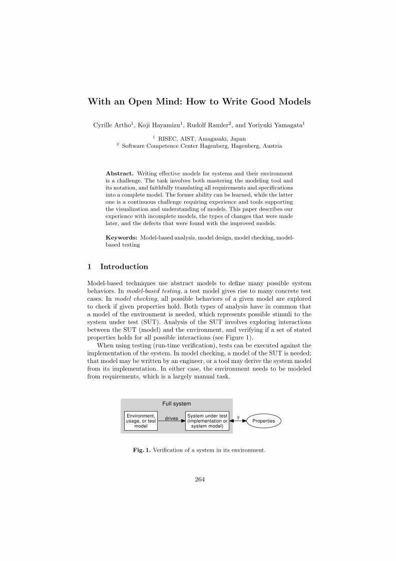
With an Open Mind: How to Write Good Models

Cyrille Artho1, Koji Hayamizu1, Rudolf Ramler2, and Yoriyuki Yamagata1

1 RISEC, AIST, Amagasaki, Japan2 Software Competence Center Hagenberg, Hagenberg, Austria

Abstract. Writing effective models for systems and their environmentis a challenge. The task involves both mastering the modeling tool andits notation, and faithfully translating all requirements and specificationsinto a complete model. The former ability can be learned, while the latterone is a continuous challenge requiring experience and tools supportingthe visualization and understanding of models. This paper describes ourexperience with incomplete models, the types of changes that were madelater, and the defects that were found with the improved models.

Keywords: Model-based analysis, model design, model checking, model-based testing

1 Introduction

Model-based techniques use abstract models to define many possible systembehaviors. In model-based testing, a test model gives rise to many concrete testcases. In model checking, all possible behaviors of a given model are exploredto check if given properties hold. Both types of analysis have in common thata model of the environment is needed, which represents possible stimuli to thesystem under test (SUT). Analysis of the SUT involves exploring interactionsbetween the SUT (model) and the environment, and verifying if a set of statedproperties holds for all possible interactions (see Figure 1).

When using testing (run-time verification), tests can be executed against theimplementation of the system. In model checking, a model of the SUT is needed;that model may be written by an engineer, or a tool may derive the system modelfrom its implementation. In either case, the environment needs to be modeledfrom requirements, which is a largely manual task.

Full system

Environment,usage, or test

model

System under test(implementation or

system model)

drivesProperties

?

Fig. 1. Verification of a system in its environment.

264

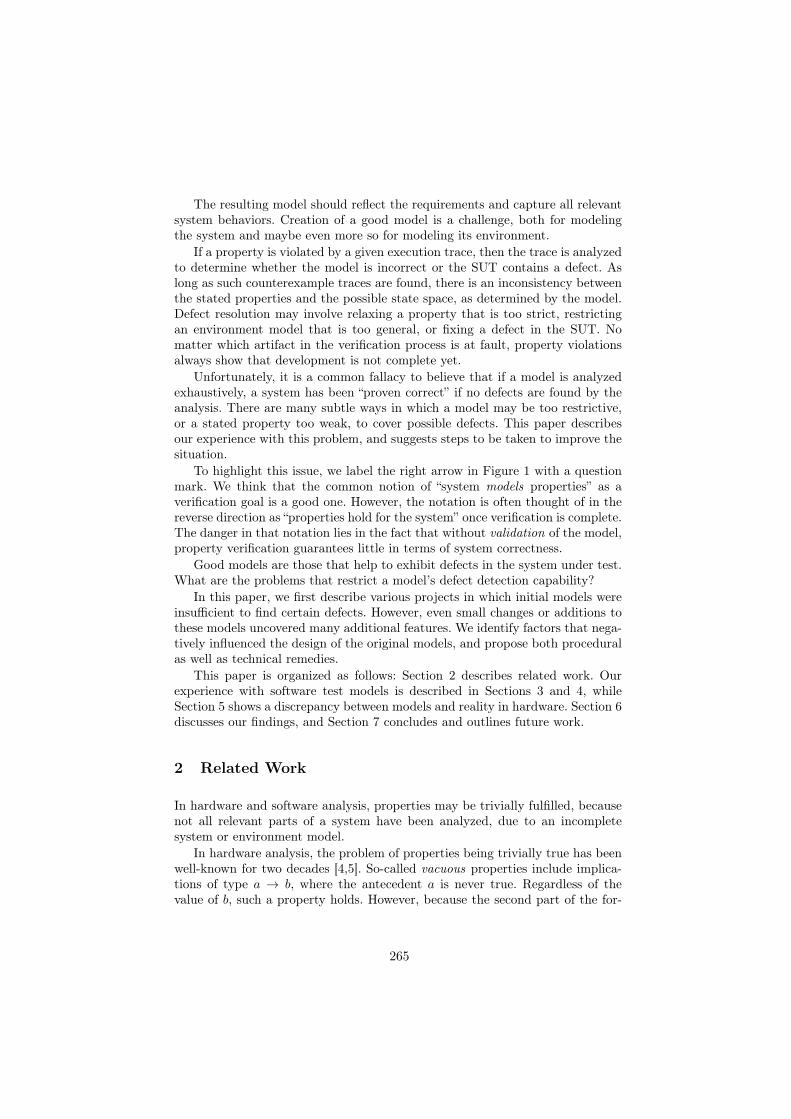
The resulting model should reflect the requirements and capture all relevantsystem behaviors. Creation of a good model is a challenge, both for modelingthe system and maybe even more so for modeling its environment.

If a property is violated by a given execution trace, then the trace is analyzedto determine whether the model is incorrect or the SUT contains a defect. Aslong as such counterexample traces are found, there is an inconsistency betweenthe stated properties and the possible state space, as determined by the model.Defect resolution may involve relaxing a property that is too strict, restrictingan environment model that is too general, or fixing a defect in the SUT. Nomatter which artifact in the verification process is at fault, property violationsalways show that development is not complete yet.

Unfortunately, it is a common fallacy to believe that if a model is analyzedexhaustively, a system has been “proven correct” if no defects are found by theanalysis. There are many subtle ways in which a model may be too restrictive,or a stated property too weak, to cover possible defects. This paper describesour experience with this problem, and suggests steps to be taken to improve thesituation.

To highlight this issue, we label the right arrow in Figure 1 with a questionmark. We think that the common notion of “system models properties” as averification goal is a good one. However, the notation is often thought of in thereverse direction as “properties hold for the system” once verification is complete.The danger in that notation lies in the fact that without validation of the model,property verification guarantees little in terms of system correctness.

Good models are those that help to exhibit defects in the system under test.What are the problems that restrict a model’s defect detection capability?

In this paper, we first describe various projects in which initial models wereinsufficient to find certain defects. However, even small changes or additions tothese models uncovered many additional features. We identify factors that nega-tively influenced the design of the original models, and propose both proceduralas well as technical remedies.

This paper is organized as follows: Section 2 describes related work. Ourexperience with software test models is described in Sections 3 and 4, whileSection 5 shows a discrepancy between models and reality in hardware. Section 6discusses our findings, and Section 7 concludes and outlines future work.

2 Related Work

In hardware and software analysis, properties may be trivially fulfilled, becausenot all relevant parts of a system have been analyzed, due to an incompletesystem or environment model.

In hardware analysis, the problem of properties being trivially true has beenwell-known for two decades [4,5]. So-called vacuous properties include implica-tions of type a → b, where the antecedent a is never true. Regardless of thevalue of b, such a property holds. However, because the second part of the for-

265

mula becomes irrelevant, this case of an “antecedent failure” is likely not whatthe modeler intended [4].

For temporal logics, so-called zeno-timelocks describe cases where parts of amodel would have to execute infinitely fast (being subject to an infinite numberof transitions in a finite amount of time) for a property to hold [8]. Such timelocksoften relate to a problem in the way parts of a system are modeled [9].

More recently, a different case, parts of a property that are unsatisfiable perse, has been investigated [20]. This property can be used to “debug” a specifica-tion, i. e., to analyze why a specification does not hold. There is emerging workin the field of diagnosing model checker specifications using scenarios to analyzethe model [17].

In software testing, modified condition/decision coverage (MC/DC) and sim-ilar test coverage criteria try to ensure that each part of a complex conditionalstatement is actually relevant for the outcome of a test suite [1,26]. For each loca-tion in the software code where compound conditionals exist, MC/DC demandsthat, among other criteria, each condition in a decision is shown to indepen-dently affect the outcome of the decision [26]. If a condition has no effect on theoutcome of a decision, it is likely incorrect (too weak) or redundant. The appli-cation of coverage criteria on the model level is emerging work, with only a fewrelatively simple coverage criteria such as state, transition, and path coverage,being commonly used so far [1].

Work investigating how human developers write test sequences has foundthat there is a bias towards designing a test case up to a “critical” operationthat is expected to possibly fail, but not beyond [10,18]. In particular, test casesare often designed to cover possible exceptions, but tend to stop at the firstexception. This bias was confirmed in our case studies for designing models fornetwork libraries [2,3] and is described in more depth below.

Finally, the problem of model validation is also well known in model-drivenengineering [6]. In that case, the model cannot be verified but only validated;recent work suggests generating questions about model properties as a form ofsanity check [6].

3 Modeling the Java Network Library with Modbat

Even in widely used commercial software such as the Java platform [15], theofficial specification and documentation is written in English and not availableas a fully rigorous formal document. This may give rise to ambiguities. In ourexperience, the biggest challenge in using the given specification was that manydetails are implicit, making it difficult to create a faithful model that also coversall relevant behaviors.

3.1 Setting

This section concerns the use of Modbat, a model-based test tool [2], for veri-fying a custom implementation of the java.nio network application program-ming interface (API) [15]. This network library allows the use of non-blocking

266

input/output (I/O) operations. Unlike blocking operations, which suspend thecurrent thread until the full result is obtained, non-blocking variants return aresult immediately; however, the result may be incomplete, requiring that theoperation be retried for completion.

The goal of this project was to test conformance of a custom version of thejava.nio library [3] w. r. t. the official documentation [15]. The custom imple-mentation of the java.nio library is designed to run on Java PathFinder [25],which requires a model implementation of code that interacts with the environ-ment [3]. When using Modbat on this library, the model replaces the environmentand generates calls to the API of the SUT.

Modbat uses an extended finite state machine [23] as its underlying model.State transitions are labeled with actions that are defined as program code(functions implemented in Scala [14]). This program code can directly executethe system under test (in our case, parts of the Java API). In addition to that,Modbat also supports exception handling, by allowing a declaration of possibleexceptions that may result by (failed) actions. Finally, Modbat supports non-blocking I/O by allowing the specification of alternative target states to coverboth the successful and the failed (incomplete) outcome of non-blocking I/O.

open configureBlocking

bound

bind

err

accept:NotYetBoundException

closed

closenon-bl. accept

(failed)

connected

bl. acceptnon-bl. accept(successful)

closeclose

read

accept:ClosedChannelException

close

Fig. 2. Initial model for java.nio server API.

We have modeled the usage of the key classes ServerSocketChannel andSocketChannel with Modbat (see Figure 2 for the server case). Both APIs havein common that a channel object first needs to be created by calling open.Our models take the resulting state as the initial state. In the server case, thecreated object represents the ability to accept incoming connections; the object

267

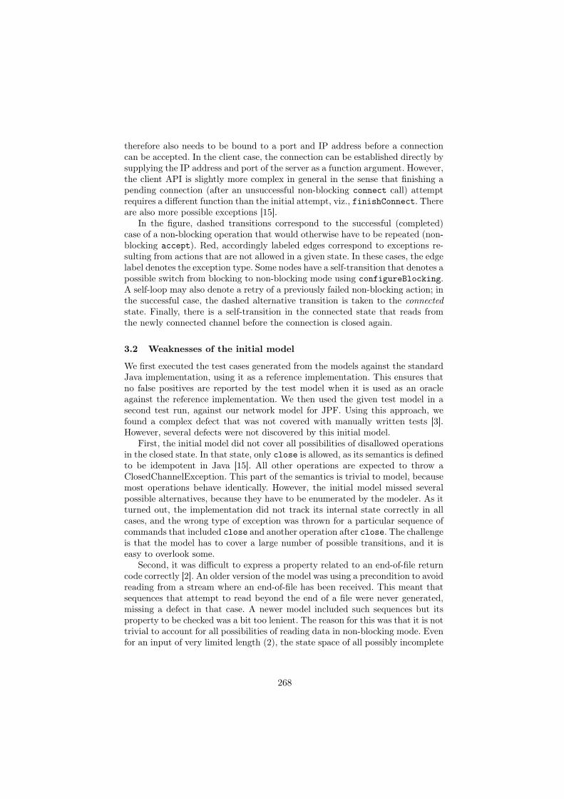
therefore also needs to be bound to a port and IP address before a connectioncan be accepted. In the client case, the connection can be established directly bysupplying the IP address and port of the server as a function argument. However,the client API is slightly more complex in general in the sense that finishing apending connection (after an unsuccessful non-blocking connect call) attemptrequires a different function than the initial attempt, viz., finishConnect. Thereare also more possible exceptions [15].

In the figure, dashed transitions correspond to the successful (completed)case of a non-blocking operation that would otherwise have to be repeated (non-blocking accept). Red, accordingly labeled edges correspond to exceptions re-sulting from actions that are not allowed in a given state. In these cases, the edgelabel denotes the exception type. Some nodes have a self-transition that denotes apossible switch from blocking to non-blocking mode using configureBlocking.A self-loop may also denote a retry of a previously failed non-blocking action; inthe successful case, the dashed alternative transition is taken to the connectedstate. Finally, there is a self-transition in the connected state that reads fromthe newly connected channel before the connection is closed again.

3.2 Weaknesses of the initial model

We first executed the test cases generated from the models against the standardJava implementation, using it as a reference implementation. This ensures thatno false positives are reported by the test model when it is used as an oracleagainst the reference implementation. We then used the given test model in asecond test run, against our network model for JPF. Using this approach, wefound a complex defect that was not covered with manually written tests [3].However, several defects were not discovered by this initial model.

First, the initial model did not cover all possibilities of disallowed operationsin the closed state. In that state, only close is allowed, as its semantics is definedto be idempotent in Java [15]. All other operations are expected to throw aClosedChannelException. This part of the semantics is trivial to model, becausemost operations behave identically. However, the initial model missed severalpossible alternatives, because they have to be enumerated by the modeler. As itturned out, the implementation did not track its internal state correctly in allcases, and the wrong type of exception was thrown for a particular sequence ofcommands that included close and another operation after close. The challengeis that the model has to cover a large number of possible transitions, and it iseasy to overlook some.

Second, it was difficult to express a property related to an end-of-file returncode correctly [2]. An older version of the model was using a precondition to avoidreading from a stream where an end-of-file has been received. This meant thatsequences that attempt to read beyond the end of a file were never generated,missing a defect in that case. A newer model included such sequences but itsproperty to be checked was a bit too lenient. The reason for this was that it is nottrivial to account for all possibilities of reading data in non-blocking mode. Evenfor an input of very limited length (2), the state space of all possibly incomplete

268

connected

read() == 0

read_1read() == 1

read() == 0

read_2read() == 1

read() == 0

eofread() == -1

read() == -1

Fig. 3. Model of end-of-file semantics; dashed transitions are incomplete reads.

read operations that eventually lead to the end-of-file is quite large (see Figure 3).The property was initially written programmatically, and the code did not trackthe internal state strictly enough under all possible circumstances; Figure 4 showshow a unit test that includes repeated calls to readByte and checks the result ina case where the input has length 2. Most of the code, including a counter anda flag, is devoted to expressing the property. As Figure 3 shows, a finite-statemachine can express the property much more succinctly [2].

SocketChannel sc = connect();sc.configureBlocking(false);int n = 0;boolean eof = false;while (n < 4) {

int read = readByte(sc);if (eof) assert (read == -1); // ensure no 0 non-bl. read after EOFif (read == -1) eof = true;if (read != 0) { // ignore non-bl. zero-reads

if (n++ < 2) { // read data twiceassert (read == 1);

} else { // always read EOF after thatassert (read == -1);

} } }sc.close();

Fig. 4. Unit test including the end-of-file property.

Third, the initial model was also limited in that it included an error state forall cases where an exception has occurred [2]. This limits test cases to executeonly up to a possible exception, but not beyond it. The reasoning behind this isthat a well-behaved user of a library never triggers an exception due to incor-rect use, of the types specified in the model. However, a component (an objectprovided by the SUT) can usually survive an incorrect command by refusingto execute it and throwing an exception instead. Because of this, it is possibleto continue a test beyond such a step, issuing more correct or incorrect com-mands. This situation tends to be overlooked when modeling the environmentof a system. Earlier case studies have shown that this is a common human biasin testing [10,18], and this has also carried over to modeling. While there in-deed exist common cases where an object cannot be used after an exception has

269

been thrown, this is not the case for incorrect operations used on communicationchannels.3 In the updated server model (see Figure 5), a trace can include otheroperations (or the same one) after a given operation resulted in an exception.

open configureBlocking accept: NotYetBoundException

bound

bind

closed

closenon-bl. accept

(failed)

connected

bl. acceptnon-bl. accept(successful)

closeclose

read bind, accept, read, configureBlocking: ClosedChannelException

close

Fig. 5. Improved model for java.nio server API.

3.3 Summary

We found three problems with an initial model for a complex API in Java. Thefirst problem was caused by the model not including all possible alternatives.The second problem was caused by a property that cannot be easily expressedin code, but where a finite-state machine may capture its semantics succinctly.Finally, the third problem stemmed from a human bias that tends to focus onoperations up to a “critical” operation throwing an exception, which lead tothe model being restricted by using an error state as a global target state for allexceptions. Instead, a self-loop should have been used to allow traces to continuebeyond an exception.

4 Experiences with Models for Testing Collection Classes

4.1 Setting

In a series of experiments we studied the effectiveness of tool-supported testcase generation in comparison to humans developing unit tests [18,19]. The ex-periment was based on a library of collection classes (i. e., containers such aslist, array, set, stack, and map) with manually seeded defects. The library weused resembles the common Java collection classes. Thus, the study material had3 On the other hand, a communication channel is usually in an unrecoverable stateafter an exception thrown due to an I/O failure.

270

the benefit of being well known by the study participants and did not requireadditional background information or familiarization. The size of the librarywas about 2,800 lines of Java code distributed to 34 classes and interfaces anda total of 164 methods. Most classes showed high algorithmic complexity andused object-oriented concepts such as interfaces, abstract classes, inheritance,polymorphism and dynamic binding.

In this context, we also briefly looked into the possibilities of model-basedapproaches for unit testing [23] and developed some preliminary ideas about howto construct models for our collection classes. However, model-based testing wasnot part of one of our studies so far and, thus, the initial models have not beenevaluated further. In the following, we document our observations about someof the challenges involved in constructing these initial models.

4.2 Modeling Test Scenarios

The starting point of our modeling attempts was the focus on developing unittest suites for the collection classes. The main motivation was to reduce themanual effort involved in implementing unit tests by automatically generatingsome or all of the test cases. So our initial perspective on modeling was influencedby the ideas and scenarios we wanted to explore in unit testing.

One of the first models was, thus, a generalization of a specific scenario thatcan be implemented as simple unit test. The objective of this test was to add andremove elements to/from a collection and to check the corresponding size of thecollection as well as that the removed elements were those that had previouslybeen added (Fig. 6).

@Test public void testAddRemove() {LinkedList l = new LinkedList(); assertEquals(0, l.size());assertTrue(l.add("1")); assertEquals(1, l.size());assertTrue(l.add("2")); assertEquals(2, l.size());assertTrue(l.remove("1")); assertEquals(1, l.size());assertTrue(l.remove("2")); assertEquals(0, l.size());

}

Fig. 6. Exemplary unit test capturing a specific sequence of add/remove operations.

This test implements one specific, representative case out of the many pos-sible sequences in which elements may be added and removed. The model weinitially developed still focused on the particular scenario of adding and removingelements (see Fig. 7).

Yet with the help of this model, we were able to generate a huge set of testcases that covered a wide range of combinations in which elements were addedand removed, eventually including also all the combinations implemented in themanually developed test cases. Several other scenarios (e. g., using iterators orsorting) were modeled in the same way, again with the intention to explore themmore extensively with huge sets of generated tests.

271

init main counter = 0

add(++counter)

remove() == counter--

Fig. 7. Simple model for generating arbitrary sequences of add/remove operations.

A weakness all these initial models had in common was that no further defectswere revealed, other than those that already had been found by the manuallywritten unit tests. By simply transferring the unit test scenarios into test models,the resulting models were inherently limited to the underlying scenarios. Sincein our case these scenarios were already sufficiently covered by a (small) set ofmanually implemented unit test cases, the model-based testing approach wasnot able to reveal new errors.

4.3 Modeling Actions on the System Under Test

To improve the initially generated test cases and to better unleash the potentialof the model-based testing approach, we tried to advance the models towardsmore realistic usage patterns. For example, we added further actions to includeall methods exposed in the public interface of a collection class and we removedthe guards preventing invalid method calls to cover a broad range of interac-tions in addition and in combination to adding and removing elements. We alsointegrated the different small models into one large model. For example, we inte-grated the model testing iterators to make sure several iterators were used as partof a larger scenario where collections are modified concurrently. The advancedmodels actually generated new fault-revealing test cases we were not thinkingabout when manually writing tests. Eventually, thus, we reached the conclusionthat the most realistic results will be achieved by developing a model that resem-bles the complete system under test as closely as possible in favor of developingseveral more specific models that reflect only individual test scenarios.

So far we have not completed the development of a full model for the collec-tion classes. Nevertheless, we found that partial models or models at a higherlevel of abstraction are already capable of detecting some of the faults, althoughthey are not rigorous enough to detect all the faults. Incrementally developingand refining the models provides the benefit of early defect detection and allowsto balance the invested modeling effort to the achieved test results.

When proceeding towards a more complete model, we encountered anotherchallenge that still remains an open issue. With the exponentially increasingnumber of possible scenarios described by a large model, the probability to suf-ficiently cover all the known interesting scenarios and critical corner cases tendsto decrease. For example, since add and remove are equally probable, the num-ber of elements in a collection usually stays low and collections rarely grow to

272

the point where new memory is allocated. Another example is related to thespecial cases when inserting and removing list elements; the first and the lastposition of a filled list have to be treated differently and should to be covered bydedicated test cases. Yet this knowledge is not part of the model. However, sincethis knowledge is already available when creating the model, it would be usefulto include it at this point as an aid to guide test case generation in direction ofthe relevant scenarios.

4.4 Modeling Test Data

Models of collection classes usually exhibit only a small number of relevant states.We found that an important aspect of the model relates to the test data, i. e.,the data elements to be stored in the collections.

Our initial model concerning the add and remove operations used a counternrOfElements to keep track of the size of the collection and to compute itsstate, i. e., empty or filled. When adding an element to the collection, we usedthe counter as new integer object to be added. When removing an element, wecompared the obtained element with the counter to make sure the expectedelement had been returned. Thus, this simple mechanism dynamically generatedreproducible test data. To avoid that the sequential order of the elements derivedfrom the counter created unbalanced sequences, e. g., new elements are alwaysadded to the end of the collection, we used the counter as seed for a randomnumber generator.

A weakness of this first model was that it missed errors caused by mixing dataelements of different type. The containers TreeSet and TreeMap are sensitive tosuch errors as are the operations for sorting and searching in collections. Thus,the initial model did not find the related seeded defects since only comparabledata objects of type Integer were used.

We extended the initial model by creating numerous test data elements ofdifferent types when setting up the model. The data elements were stored inan array in arbitrary order. The counter we previously used in the model nowserved as array index, which still allowed to determine the expected element tobe returned by a remove operation.

Only later we found a new fault that indicated that there is still room forfurther improvement. The implementation of the collection classes was not ableto handle the case of a collection being added to itself. Some operations such astoString would then lead to an unbounded recursion (see Fig. 8). We furtherextended the model to dynamically add new data elements to the test data setnot only at startup but also while the model is executed. In future we plan toextended the model to incorporate the idea of feedback-directed test genera-tion [16].

Stack s = new Stack(); s.push(s); s.toString();

Fig. 8. Sequence revealing an unbound recursion in the implementation of Stack.

273

A related issue is involved in using null values, since the implementationof some container classes accept null as valid data elements whereas others donot. This issue was found when we tried to reuse generic models for differentcontainer classes. This observation led us to the (ongoing) discussion to whatextent a model should reflect the behavior of the system under test versus itsenvironment, i. e., the allowable inputs from the anticipated usage. While Uttinget al. [24] classify this scope as a binary decision (input-only versus input-outputmodels), we found that our models always combined both sides since modelingthe input side also required some knowledge about the expected output.

4.5 Summary

We reported on work on modeling the behavior of Java container classes. Initialmodels that were created from generalizations of existing unit tests ended upnot being effective at finding defects that were not already covered by unittests. When extending these models, we found that models that are convenientto define (for example, using only numbers) end up not covering importantcases such as different data types or null values. Finally, creating modular andreusable models is difficult, because small differences in components result inpervasive differences in the allowable inputs requiring extra effort to adjust.

5 Industrial Project: Electric Circuit

5.1 Adapted work flow

As described in Section 2, various subtleties regarding the aspects of timed mod-els and the reachability of model and system states in hardware are known. Toavoid incorrect models, verification engineers validate their model with domainexperts, who design the circuit. In this project, we employed the following workflow to eliminate false positives (spurious warnings) and false negatives (misseddefects):

1. For a set of given desired states, reachability of these states is checked. Forexample, any terminal state in the system should be reachable.

2. The specification is negated and model checked. This means that the modelchecker analyzes whether there exist paths in the model that fulfill the de-sired property. In a correct model, correct execution paths should be gener-ated. These execution paths are generated as counterexamples by the modelchecker, as the real property has been negated. Different counterexamplepaths are subsequently reviewed together with domain experts to determinewhether they are correct and reflect the expected behavior of the system.

3. Properties that are trivially expected to hold are checked as well, as a formof sanity check.

274

5.2 Problem found

The work flow described above prevents many defects in the model. However,despite this, a modeling problem was found in an industrial project on an electriccircuit. The problem is related to how time is modeled in a real system. Thesystem model uses discrete time, where the state of each component is updatedon the next model clock tick. However, in real hardware, components can changetheir state almost immediately; the “slowness” introduced by discrete time gaverise to a counter-example in this model (see Figure 9). The problem in thismodel is that gSet_PT_Voltage_A01 is updated in the next state even thoughthe voltage change is immediate in real hardware.

next(gSet_PT_Voltage_A01) := caseGen_to_Load_A = 0 & Brk_A = 0 & GL_V_A = 0 & LG_V_A = 0 : V_Emp;Gen_to_Load_A = 0 & Brk_A = 0 & GL_V_A = 0 & LG_V_A = 1 : V_Lrd;Gen_to_Load_A = 0 & Brk_A = 0 & GL_V_A = 1 & LG_V_A = 0 : V_Gen;...

esac;

Fig. 9. Part of a model transition describing an industrial circuit.

After the counterexample was investigated together with domain experts, itwas considered to be spurious (a false positive). To fix the model, the first linein the model was amended to gSet_PT_Voltage_A01 := case (i. e., next wasremoved). This eliminated the false positive.

6 Discussion

We have reported our experience from several modeling projects. In each project,there were unexpected problems with creating a correct and sufficiently goodmodel to fulfill the purpose of model-based verification. In our opinion, it isinteresting that the problems were not caused by ambiguities of the requirementsor documentation. Where ambiguities caused problems, we were able to identifythem and clarify the open points by checking the reference implementation.

6.1 Model design

In our projects, problems arose when requirements were transformed into amodel. We often failed to create a model that matches a wide range of all possiblebehaviors stated in the requirements. All of the models were “correct” but failedto cover certain behaviors of the system, some of which were even implementedincorrectly. In the software projects, the uncovered behaviors resulted in misseddefects (false negatives); in the hardware project, it resulted in a spurious error(false positive), which gives an indication of a mismatch between the model andreality.

275

The lack of expressiveness in the models did not originate from unintendederrors or oversights, but from intentional abstractions or decisions that led toelegant models. The resulting lack of coverage was therefore a side-effect of con-scious design decisions. From this observation, we identify the right level ofabstraction and human bias [10] as the key problems.

Abstraction. A major problem of creating a good model is to choose the rightlevel of abstraction. This is a very difficult problem that takes years of experienceto solve well. Some people even claim that this skill may not be teachable butan innate ability [12]. In the future, we expect (modeling/abstraction) teachingmethods, and design tools, to improve to make the task a bit less daunting.

Human bias. When choosing an abstraction, human bias also often exists inthat the model is designed for a narrower purpose than necessary. This leadsto the omission of certain behaviors in the model. Like abstraction, this is afundamentally difficult problem to overcome; it requires to attack the problemfrom various angles to obtain a comprehensive solution. We think that involvinga team of people in modeling, and making an effort to avoid any preconception,can at least mitigate this problem. Ideally, models are created with an open, freshmind, and no possibilities, regardless of being difficult or trivial to handle, shouldbe disregarded. In practice, this may require careful engineering of the modelw .r. t. code reuse, if one takes into account that many small subtle differencesin system components result in a large increase of different possible behaviors(and thus models or parameterizations thereof).

6.2 Model validation

Our experience shows that model-based verification has to be grounded in anextensive validation of the model. Even though validation is in itself not a fullymechanized activity, there exists tool support for tasks such as coverage analysisand visualization, which contribute to validation. Furthermore, computer sup-port can also be used in the modeling stage itself if certain artifacts such as areference implementation are available.

Machine learning. Machine learning of models has the obvious advantage ofnot missing system states due to a simple oversight. If a correct (reference)implementation of a system exists, then a model can be derived from the existingsystem using machine learning [21,13]. The resulting model may not be human-readable but its verification verdict may confirm or refute the result obtainedfrom a model designed by a human.

This approach can even be used if it is not known if a given system is correct;in that case, the model reflects its current (possibly not fully correct) behaviorand can be used in regression testing to see if the behavior of the system changesin unexpected ways. Changes that violate a given property then would likely befound by a model that reflects the semantics of an older (“known good”) versionof the system.

276

Diagnosis and visualization. Some of the weaknesses observed in models arosefrom the fact that they were generalizations of existing test scenarios. Therefore,just lifting a set of execution traces to a grammar-based model is not guaran-teed to add much value. It is also necessary to check whether the existing testscenarios, and the derived model, are comprehensive enough.

We therefore advocate that model-based verification be combined with modeldiagnosis and visualization, so possible flaws in a model learned from an incom-plete set of tests, or a defective system, may be found. In our hardware project,we already had adapted such a workflow by checking a sample of all possibleexecution traces generated by the model checker.

Model coverage and mutation analysis. It is important to analyze the cover-age of the model in the real system; this can be done for software testing in astraightforward way [1,26]. However, coverage analysis on the final product givesus limited information on the expressiveness of the model itself (in addition tonot being able to tell us whether all requirements are actually met). Hence, wealso advocate mutation operators for models to find mutants that still pass theproperties.

Mutating model properties is well-known [7] (and very similar to programcode [11]). However, work needs to be done on mutating the structure of themodel: a model could also be mutated by duplicating or deleting a transition, orchanging its source or target state. This reflects what we have learned from oursoftware model, where the model structure itself (and not just a given predicateor property) restricted its behavior.

Combination of model-based and model-free techniques. When analyzing the im-plementation of a system, fully automated analysis techniques can complementhuman efforts. Unlike in the case where a model is designed by a human, auto-mated techniques have no test oracle that evaluates the output of the analyzedbehaviors; instead, they serve as a “sanity check” for a wide range of genericproperties (accessed memory must be initialized, no deadlocks, etc.).

When using such “model-free” techniques, randomized testing [16] often findsdefects that humans miss [18]. Defects found by such tools may in turn spur animprovement in a manually written model. A comparison of the states coveredby model-free techniques with the coverage of a manually written model, mayunveil weaknesses in the latter as well.

7 Conclusions and Future Work

Writing good models is a challenge. Models should not only be correct but suffi-ciently expressive and inclusive to fulfill the purpose of finding defects or ensuringtheir absence. Finding the right level of abstraction, and trying to avoid humanbias, or two of the key challenges in this process. A high level of abstractionthat allows an efficient encoding of a model (or reuse of existing model code)may not cover enough details of all possible behaviors. Modeling languages and

277

tools should strive to improve this trade-off. Teaching engineers about commonlyencountered problems or human bias is also essential.

We have listed several non-trivial flaws that we found in existing model de-velopment projects, and we have given suggestions how these may be avoidedin the future. Tool-supported analysis of the model itself will help to explorethe system behavior in its full breadth and may uncover missing model aspectsthat human inspection misses. In this context, we advocate using model-free,automated approaches where possible, so that their coverage can be comparedwith the coverage yielded by a model derived from the specification.

We believe that more case studies can also shed more light into why certainproperties tend to be forgotten, and what types of modeling challenges engineerstypically encounter. This may eventually lead to the creation of a body of knowl-edge for modeling and its effective use in practice. Existing work tends to focuson surveying approaches and tools, such as MCBOK, a body of knowledge onmodel checking for software development [22]; we hope that more fundamentalcognitive and process-level issues will also be covered in the future.

Acknowledgments. We would like to thank Takashi Kitamura and KenjiTaguchi for their suggestions on this paper.

References

1. P. Ammann and J. Offutt. Introduction to Software Testing. Cambridge UniversityPress, New York, USA, 1 edition, 2008.

2. C. Artho, A. Biere, M. Hagiya, E. Platon, M. Seidl, Y. Tanabe, and M. Yamamoto.Modbat: A model-based API tester for event-driven systems. In Proc. 9th HaifaVerification Conference (HVC 2013), LNCS, Haifa, Israel, 2013. Springer. To bepublished.

3. C. Artho, M. Hagiya, R. Potter, Y. Tanabe, F. Weitl, and M. Yamamoto. Softwaremodel checking for distributed systems with selector-based, non-blocking commu-nication. In Proc. 28th Int. Conf. on Automated Software Engineering (ASE 2013),Palo Alto, USA, 2013.

4. D. Beatty and R. Bryant. Formally verifying a microprocessor using a simulationmethodology. In Proc. 31st Conf. on Design Automation (DAC 1994), pages 596–602, San Diego, USA, 1994.

5. I. Beer, S. Ben-David, C. Eisner, and A. Landver. Rulebase: An industry-orientedformal verification tool. In Proc. 33rd Conf. on Design Automation (DAC 1996),pages 655–660, Las Vegas, USA, 1996.

6. A. Bertolino, G. De Angelis, A. Di Sandro, and A. Sabetta. Is my model right? letme ask the expert. J. Syst. Softw., 84(7):1089–1099, July 2011.

7. P. Black, V. Okun, and Y. Yesha. In E. Wong, editor, Mutation testing for the newcentury, chapter Mutation of model checker specifications for test generation andevaluation, pages 14–20. Kluwer Academic Publishers, Norwell, MA, USA, 2001.

8. H. Bowman. How to stop time stopping. Form. Asp. Comput., 18(4):459–493,2006.

9. H. Bowman, G. Faconti, J-P. Katoen, D. Latella, and M. Massink. Automaticverification of a lip synchronisation algorithm using UPPAAL. In Proc. 3rd Int.

278

Workshop on Formal Methods for Industrial Critical Systems, pages 97–124. CWI,1998.

10. G. Calikli and A. Bener. Empirical analyses of the factors affecting confirma-tion bias and the effects of confirmation bias on software developer/tester per-formance. In Proc. 6th Int. Conf. on Predictive Models in Software Engineering,PROMISE 2010, pages 10:1–10:11, New York, NY, USA, 2010. ACM.

11. Yue J. and Mark H. An analysis and survey of the development of mutation testing.Software Engineering, IEEE Transactions on, 37(5):649–678, 2011.

12. J. Kramer. Is abstraction the key to computing? Commun. ACM, 50(4):36–42,April 2007.

13. A. Memon and B. Nguyen. Advances in automated model-based system testing ofsoftware applications with a GUI front-end. Advances in Computers, 80:121–162,2010.

14. M. Odersky, L. Spoon, and B. Venners. Programming in Scala: A ComprehensiveStep-by-step Guide. Artima Inc., USA, 2nd edition, 2010.

15. Oracle. Java Platform Standard Edition 7 API Specification, 2013.http://docs.oracle.com/javase/7/docs/api/.

16. C. Pacheco, S. Lahiri, M. Ernst, and T. Ball. Feedback-directed random testgeneration. In Proc. 29th Int. Conf. on Softw. Eng., ICSE 2007, pages 75–84,Washington, DC, USA, 2007. IEEE Computer Society.

17. I. Pill and T. Quaritsch. Behavioral diagnosis of LTL specifications at operatorlevel. In Proc. 23rd Int. Joint Conf. on Artificial Intelligence (IJCAI 2013), Beijing,China, 2013. IJCAI/AAAI.

18. R. Ramler, D. Winkler, and M. Schmidt. Random test case generation and manualunit testing: Substitute or complement in retrofitting tests for legacy code? In 36thConf. on Software Engineering and Advanced Applications, pages 286–293. IEEEComputer Society, 2012.

19. R. Ramler, K. Wolfmaier, and T. Kopetzky. A replicated study on random testcase generation and manual unit testing: How many bugs do professional developersfind? In Proc. 37th Annual Int. Comp. Software & Applications Conf., COMPSAC2013, pages 484–491, Washington, DC, USA, 2013. IEEE Computer Society.

20. V. Schuppan. Towards a notion of unsatisfiable and unrealizable cores for LTL.Sci. Comput. Program., 77(7-8):908–939, 2012.

21. B. Steffen, F. Howar, and M. Isberner. Active automata learning: From DFAs to in-terface programs and beyond. Journal of Machine Learning Research—ProceedingsTrack, 21:195–209, 2012.

22. K. Taguchi, H. Nishihara, T. Aoki, F. Kumeno, K. Hayamizu, and K. Shinozaki.Building a body of knowledge on model checking for software development. InProc. 37th Annual International Computer Software & Applications Conf. (COMP-SAC 2013), Kyoto, Japan, 2013. IEEE.

23. M. Utting and B. Legeard. Practical Model-Based Testing: A Tools Approach.Morgan Kaufmann Publishers, Inc., San Francisco, USA, 2006.

24. M. Utting, A. Pretschner, and B. Legeard. A taxonomy of model-based testingapproaches. Softw. Test. Verif. Reliab., 22(5):297–312, August 2012.

25. W. Visser, K. Havelund, G. Brat, S. Park, and F. Lerda. Model checking programs.Automated Software Engineering Journal, 10(2):203–232, 2003.

26. Y. Yu and M. Lau. A comparison of MC/DC, MUMCUT and several other coveragecriteria for logical decisions. J. Syst. Softw., 79(5):577–590, May 2006.

279