the influence of internal friction on rotordynamic instability
341
Rotordynamic Modeling
and Analysis
6
6.1 Analytical Models and Essential Components
The analytical prediction of the rotor dynamic behavior and bearing performance depends
heavily on accurately modeling the physical system and understanding the assumptions
and limitations applied in the modeling and analytical tools employed. The modeling of
complicated rotating machinery, however, relies on sound engineering judgment and
practical experience. The modeling process transforms the complex physical system into
a representative, hopefully simple, mathematical model. The connections between the
physical system and the mathematical model must be understood well enough, so that the
results obtained from the mathematical analysis can be verified and fully utilized in the
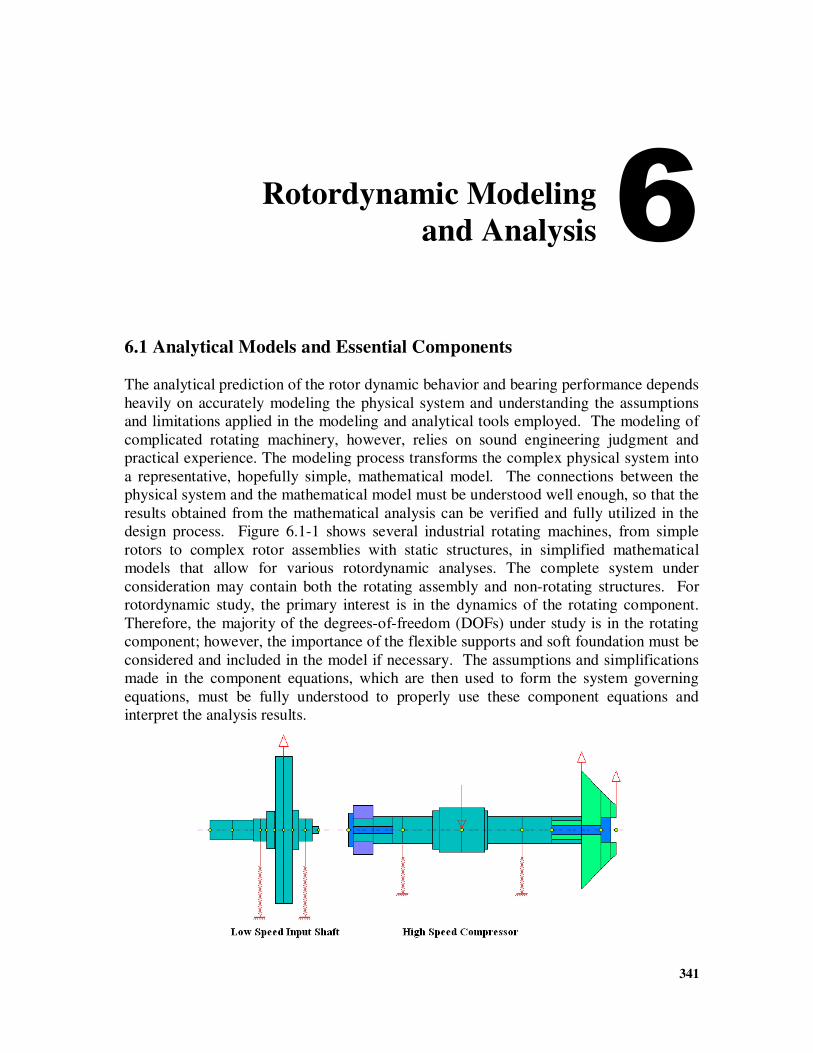
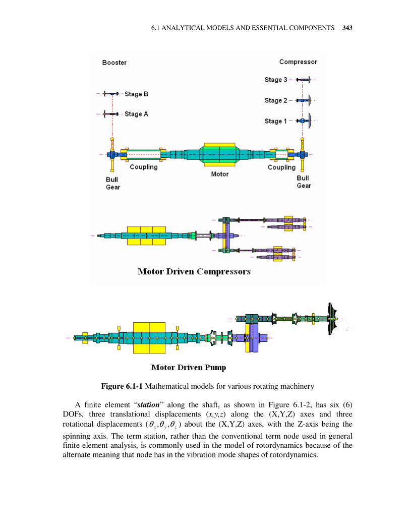
design process. Figure 6.1-1 shows several industrial rotating machines, from simple
rotors to complex rotor assemblies with static structures, in simplified mathematical
models that allow for various rotordynamic analyses. The complete system under
consideration may contain both the rotating assembly and non-rotating structures. For
rotordynamic study, the primary interest is in the dynamics of the rotating component.
Therefore, the majority of the degrees-of-freedom (DOFs) under study is in the rotating
component; however, the importance of the flexible supports and soft foundation must be
considered and included in the model if necessary. The assumptions and simplifications
made in the component equations, which are then used to form the system governing
equations, must be fully understood to properly use these component equations and
interpret the analysis results.
CHAPTER 6: ROTORDYNAMIC MODELING AND ANALYSIS
342
6.1 ANALYTICAL MODELS AND ESSENTIAL COMPONENTS
343
Figure 6.1-1 Mathematical models for various rotating machinery
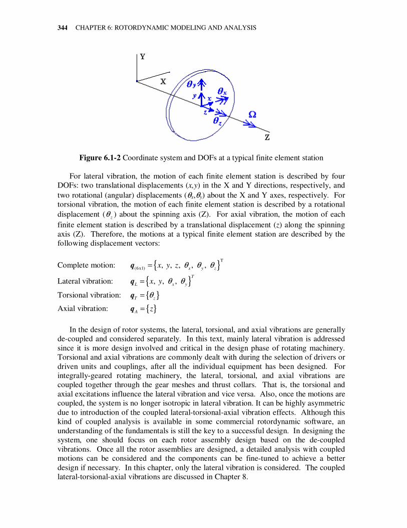
A finite element “station” along the shaft, as shown in Figure 6.1-2, has six (6)
DOFs, three translational displacements (x,y,z) along the (X,Y,Z) axes and three
rotational displacements ( zyx θθθ ,, ) about the (X,Y,Z) axes, with the Z-axis being the
spinning axis. The term station, rather than the conventional term node used in general
finite element analysis, is commonly used in the model of rotordynamics because of the
alternate meaning that node has in the vibration mode shapes of rotordynamics.
CHAPTER 6: ROTORDYNAMIC MODELING AND ANALYSIS
344
Figure 6.1-2 Coordinate system and DOFs at a typical finite element station
For lateral vibration, the motion of each finite element station is described by four
DOFs: two translational displacements (x,y) in the X and Y directions, respectively, and
two rotational (angular) displacements (θx,θy) about the X and Y axes, respectively. For
torsional vibration, the motion of each finite element station is described by a rotational
displacement ( zθ ) about the spinning axis (Z). For axial vibration, the motion of each
finite element station is described by a translational displacement (z) along the spinning
axis (Z). Therefore, the motions at a typical finite element station are described by the
following displacement vectors:
Complete motion: T
(6x1) , , , , , x y z
x y z θ θ θ=q
Lateral vibration: , , , T
L x yx y θ θ=q
Torsional vibration: T zθ=q
Axial vibration: Az=q
In the design of rotor systems, the lateral, torsional, and axial vibrations are generally
de-coupled and considered separately. In this text, mainly lateral vibration is addressed
since it is more design involved and critical in the design phase of rotating machinery.
Torsional and axial vibrations are commonly dealt with during the selection of drivers or
driven units and couplings, after all the individual equipment has been designed. For
integrally-geared rotating machinery, the lateral, torsional, and axial vibrations are
coupled together through the gear meshes and thrust collars. That is, the torsional and
axial excitations influence the lateral vibration and vice versa. Also, once the motions are
coupled, the system is no longer isotropic in lateral vibration. It can be highly asymmetric
due to introduction of the coupled lateral-torsional-axial vibration effects. Although this
kind of coupled analysis is available in some commercial rotordynamic software, an
understanding of the fundamentals is still the key to a successful design. In designing the
system, one should focus on each rotor assembly design based on the de-coupled
vibrations. Once all the rotor assemblies are designed, a detailed analysis with coupled
motions can be considered and the components can be fine-tuned to achieve a better
design if necessary. In this chapter, only the lateral vibration is considered. The coupled
lateral-torsional-axial vibrations are discussed in Chapter 8.
6.1 ANALYTICAL MODELS AND ESSENTIAL COMPONENTS
345
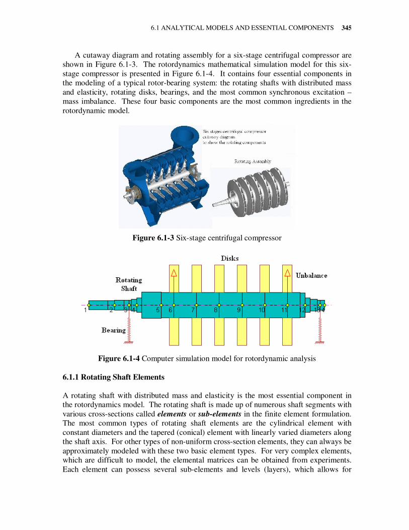
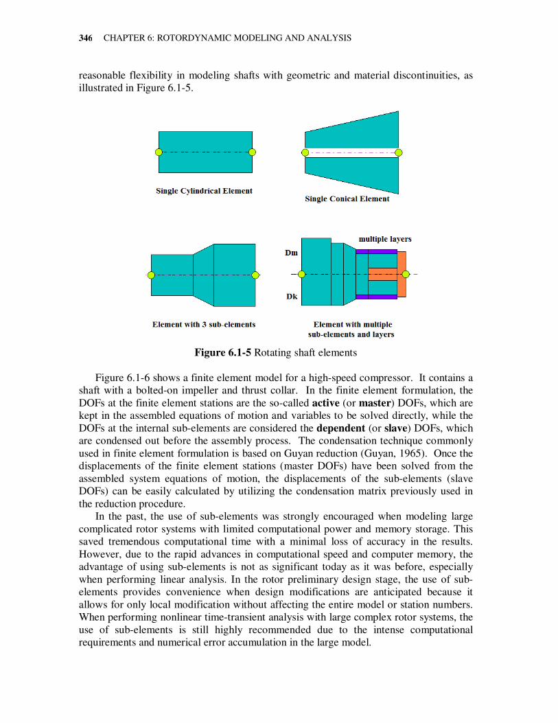
A cutaway diagram and rotating assembly for a six-stage centrifugal compressor are
shown in Figure 6.1-3. The rotordynamics mathematical simulation model for this six-
stage compressor is presented in Figure 6.1-4. It contains four essential components in
the modeling of a typical rotor-bearing system: the rotating shafts with distributed mass
and elasticity, rotating disks, bearings, and the most common synchronous excitation –
mass imbalance. These four basic components are the most common ingredients in the
rotordynamic model.
Figure 6.1-3 Six-stage centrifugal compressor
Figure 6.1-4 Computer simulation model for rotordynamic analysis
6.1.1 Rotating Shaft Elements
A rotating shaft with distributed mass and elasticity is the most essential component in
the rotordynamics model. The rotating shaft is made up of numerous shaft segments with
various cross-sections called elements or sub-elements in the finite element formulation.
The most common types of rotating shaft elements are the cylindrical element with
constant diameters and the tapered (conical) element with linearly varied diameters along
the shaft axis. For other types of non-uniform cross-section elements, they can always be
approximately modeled with these two basic element types. For very complex elements,
which are difficult to model, the elemental matrices can be obtained from experiments.
Each element can possess several sub-elements and levels (layers), which allows for
CHAPTER 6: ROTORDYNAMIC MODELING AND ANALYSIS
346
reasonable flexibility in modeling shafts with geometric and material discontinuities, as
illustrated in Figure 6.1-5.
Figure 6.1-5 Rotating shaft elements
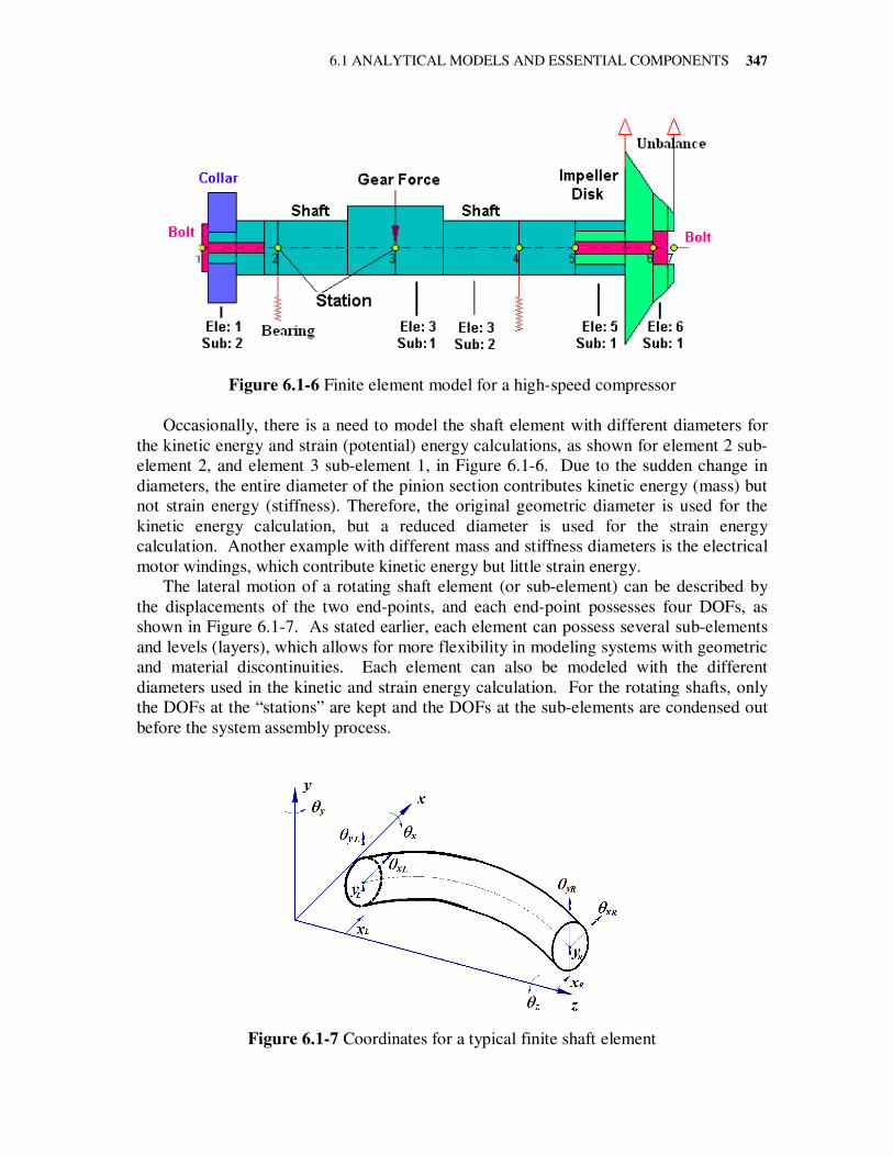
Figure 6.1-6 shows a finite element model for a high-speed compressor. It contains a
shaft with a bolted-on impeller and thrust collar. In the finite element formulation, the
DOFs at the finite element stations are the so-called active (or master) DOFs, which are
kept in the assembled equations of motion and variables to be solved directly, while the
DOFs at the internal sub-elements are considered the dependent (or slave) DOFs, which
are condensed out before the assembly process. The condensation technique commonly
used in finite element formulation is based on Guyan reduction (Guyan, 1965). Once the
displacements of the finite element stations (master DOFs) have been solved from the
assembled system equations of motion, the displacements of the sub-elements (slave
DOFs) can be easily calculated by utilizing the condensation matrix previously used in
the reduction procedure.
In the past, the use of sub-elements was strongly encouraged when modeling large
complicated rotor systems with limited computational power and memory storage. This
saved tremendous computational time with a minimal loss of accuracy in the results.
However, due to the rapid advances in computational speed and computer memory, the
advantage of using sub-elements is not as significant today as it was before, especially
when performing linear analysis. In the rotor preliminary design stage, the use of sub-
elements provides convenience when design modifications are anticipated because it
allows for only local modification without affecting the entire model or station numbers.
When performing nonlinear time-transient analysis with large complex rotor systems, the
use of sub-elements is still highly recommended due to the intense computational
requirements and numerical error accumulation in the large model.
6.1 ANALYTICAL MODELS AND ESSENTIAL COMPONENTS
347
Figure 6.1-6 Finite element model for a high-speed compressor
Occasionally, there is a need to model the shaft element with different diameters for
the kinetic energy and strain (potential) energy calculations, as shown for element 2 sub-
element 2, and element 3 sub-element 1, in Figure 6.1-6. Due to the sudden change in
diameters, the entire diameter of the pinion section contributes kinetic energy (mass) but
not strain energy (stiffness). Therefore, the original geometric diameter is used for the
kinetic energy calculation, but a reduced diameter is used for the strain energy
calculation. Another example with different mass and stiffness diameters is the electrical
motor windings, which contribute kinetic energy but little strain energy.
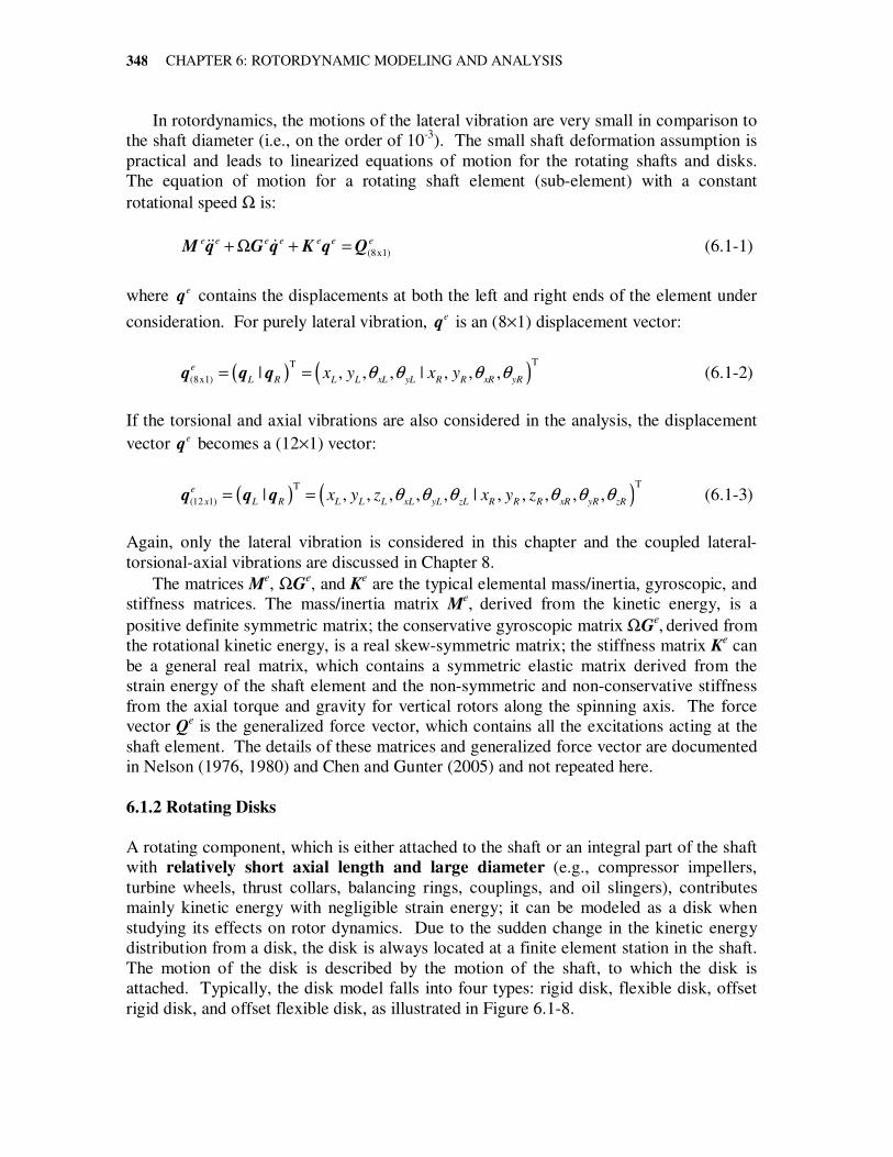
The lateral motion of a rotating shaft element (or sub-element) can be described by
the displacements of the two end-points, and each end-point possesses four DOFs, as
shown in Figure 6.1-7. As stated earlier, each element can possess several sub-elements
and levels (layers), which allows for more flexibility in modeling systems with geometric
and material discontinuities. Each element can also be modeled with the different
diameters used in the kinetic and strain energy calculation. For the rotating shafts, only
the DOFs at the “stations” are kept and the DOFs at the sub-elements are condensed out
before the system assembly process.
Figure 6.1-7 Coordinates for a typical finite shaft element
CHAPTER 6: ROTORDYNAMIC MODELING AND ANALYSIS
348
In rotordynamics, the motions of the lateral vibration are very small in comparison to
the shaft diameter (i.e., on the order of 10-3
). The small shaft deformation assumption is
practical and leads to linearized equations of motion for the rotating shafts and disks.
The equation of motion for a rotating shaft element (sub-element) with a constant
rotational speed Ω is:
(8x1)
e e e e e e e+ Ω + =M q G q K q Qɺɺ ɺ (6.1-1)
where eq contains the displacements at both the left and right ends of the element under
consideration. For purely lateral vibration, eq is an (8×1) displacement vector:
( ) ( )TT
(8x1) | , , , | , , ,e
L R L L xL yL R R xR yRx y x yθ θ θ θ= =q q q (6.1-2)
If the torsional and axial vibrations are also considered in the analysis, the displacement
vector eq becomes a (12×1) vector:
( ) ( )TT
(12 1) | , , , , , | , , , , ,e
x L R L L L xL yL zL R R R xR yR zRx y z x y zθ θ θ θ θ θ= =q q q (6.1-3)
Again, only the lateral vibration is considered in this chapter and the coupled lateral-
torsional-axial vibrations are discussed in Chapter 8.
The matrices Me, ΩG
e, and K
e are the typical elemental mass/inertia, gyroscopic, and
stiffness matrices. The mass/inertia matrix Me, derived from the kinetic energy, is a
positive definite symmetric matrix; the conservative gyroscopic matrix ΩGe, derived from
the rotational kinetic energy, is a real skew-symmetric matrix; the stiffness matrix Ke can
be a general real matrix, which contains a symmetric elastic matrix derived from the
strain energy of the shaft element and the non-symmetric and non-conservative stiffness
from the axial torque and gravity for vertical rotors along the spinning axis. The force
vector Qe is the generalized force vector, which contains all the excitations acting at the
shaft element. The details of these matrices and generalized force vector are documented
in Nelson (1976, 1980) and Chen and Gunter (2005) and not repeated here.
6.1.2 Rotating Disks
A rotating component, which is either attached to the shaft or an integral part of the shaft
with relatively short axial length and large diameter (e.g., compressor impellers,
turbine wheels, thrust collars, balancing rings, couplings, and oil slingers), contributes
mainly kinetic energy with negligible strain energy; it can be modeled as a disk when
studying its effects on rotor dynamics. Due to the sudden change in the kinetic energy
distribution from a disk, the disk is always located at a finite element station in the shaft.
The motion of the disk is described by the motion of the shaft, to which the disk is
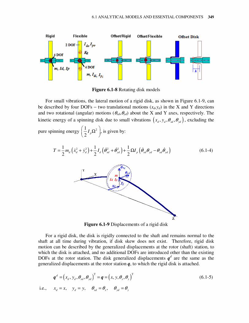
attached. Typically, the disk model falls into four types: rigid disk, flexible disk, offset
rigid disk, and offset flexible disk, as illustrated in Figure 6.1-8.
6.1 ANALYTICAL MODELS AND ESSENTIAL COMPONENTS
349
Figure 6.1-8 Rotating disk models
For small vibrations, the lateral motion of a rigid disk, as shown in Figure 6.1-9, can
be described by four DOFs − two translational motions (xd,yd) in the X and Y directions
and two rotational (angular) motions (θxd,θyd) about the X and Y axes, respectively. The
kinetic energy of a spinning disk due to small vibrations ( ), , ,d d xd yd
x y θ θ , excluding the
pure spinning energy 21
2pI
Ω
, is given by:
( ) ( ) ( )2 2 2 21 1 1
2 2 2d d d d xd yd p xd yd xd yd
T m x y I Iθ θ θ θ θ θ= + + + + Ω −ɺ ɺ ɺ ɺɺ ɺ (6.1-4)
Figure 6.1-9 Displacements of a rigid disk
For a rigid disk, the disk is rigidly connected to the shaft and remains normal to the
shaft at all time during vibration, if disk skew does not exist. Therefore, rigid disk
motion can be described by the generalized displacements at the rotor (shaft) station, to
which the disk is attached, and no additional DOFs are introduced other than the existing
DOFs at the rotor station. The disk generalized displacements qd are the same as the
generalized displacements at the rotor station q, to which the rigid disk is attached.
( ) ( )T T
, , , , , ,d
d d xd yd x yx y x yθ θ θ θ= = =q q (6.1-5)
i.e., , , , d d xd x yd y
x x y y θ θ θ θ= = = =
CHAPTER 6: ROTORDYNAMIC MODELING AND ANALYSIS
350
Hence, no additional DOF is introduced for a rigid disk. The governing equation of
motion for a rotating rigid disk (4DOF), with a constant rotational speed Ω in the fixed
reference frame, can be derived from the Lagrange’s equation:
(4 1)
d d d
x+ Ω =M q G q Qɺɺ ɺ (6.1-6)
The (4×1) rigid disk generalized displacements are replaced by the generalized
displacements at the rotor station, to which the rigid disk is attached. The mass/inertia
matrix Md, derived from the kinetic energy, is a positive definite symmetric matrix; the
conservative gyroscopic matrix ΩGd, derived from the rotational kinetic energy, is a real
skew-symmetric matrix that cross-couples the two rotational DOFs (θx, θy). Qd is the
generalized force vector, which contains all the excitations acting at the disk center of
mass and the gravity loading due to disk mass. Again, the derivations of the above
matrices and vector are well documented in previous publications (Nelson, 1976, 1980;
Chen & Gunter, 2005), and are not repeated here.
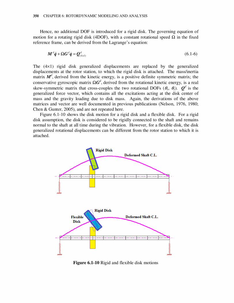
Figure 6.1-10 shows the disk motion for a rigid disk and a flexible disk. For a rigid
disk assumption, the disk is considered to be rigidly connected to the shaft and remains
normal to the shaft at all time during the vibration. However, for a flexible disk, the disk
generalized rotational displacements can be different from the rotor station to which it is
attached.
Figure 6.1-10 Rigid and flexible disk motions
6.1 ANALYTICAL MODELS AND ESSENTIAL COMPONENTS
351
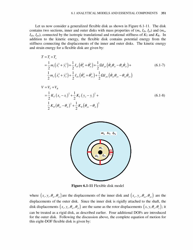
Let us now consider a generalized flexible disk as shown in Figure 6.1-11. The disk
contains two sections, inner and outer disks with mass properties of (mi, Idi, Ipi) and (mo,
Ido, Ipo), connected by the isotropic translational and rotational stiffness of KT and KR. In
addition to the kinetic energy, the flexible disk contains potential energy from the
stiffness connecting the displacements of the inner and outer disks. The kinetic energy
and strain energy for a flexible disk are given by:
( ) ( ) ( )
( ) ( ) ( )
2 2 2 2
2 2 2 2
1 1 1
2 2 2
1 1 1 2 2 2
i o
i i i di xi yi pi xi yi xi yi
o o o do xo yo po xo yo xo yo
T T T
m x y I I
m x y I I
θ θ θ θ θ θ
θ θ θ θ θ θ
= +
= + + + + Ω − +
+ + + + Ω −
ɺ ɺ ɺ ɺɺ ɺ
ɺ ɺ ɺ ɺɺ ɺ
(6.1-7)
( ) ( )
( ) ( )
2 2
22
1 1
2 2
1 1 2 2
T R
T o i T o i
R xo xi R yo yi
V V V
K x x K y y
K Kθ θ θ θ
= +
= − + − +
− + −
(6.1-8)
Figure 6.1-11 Flexible disk model
where ( ), , ,i i xi yi
x y θ θ are the displacements of the inner disk and ( ), , ,o o xo yo
x y θ θ are the
displacements of the outer disk. Since the inner disk is rigidly attached to the shaft, the
disk displacements ( ), , ,i i xi yi
x y θ θ are the same as the rotor displacements ( ), , ,x y
x y θ θ ; it
can be treated as a rigid disk, as described earlier. Four additional DOFs are introduced
for the outer disk. Following the discussion above, the complete equation of motion for
this eight-DOF flexible disk is given by:
CHAPTER 6: ROTORDYNAMIC MODELING AND ANALYSIS
352
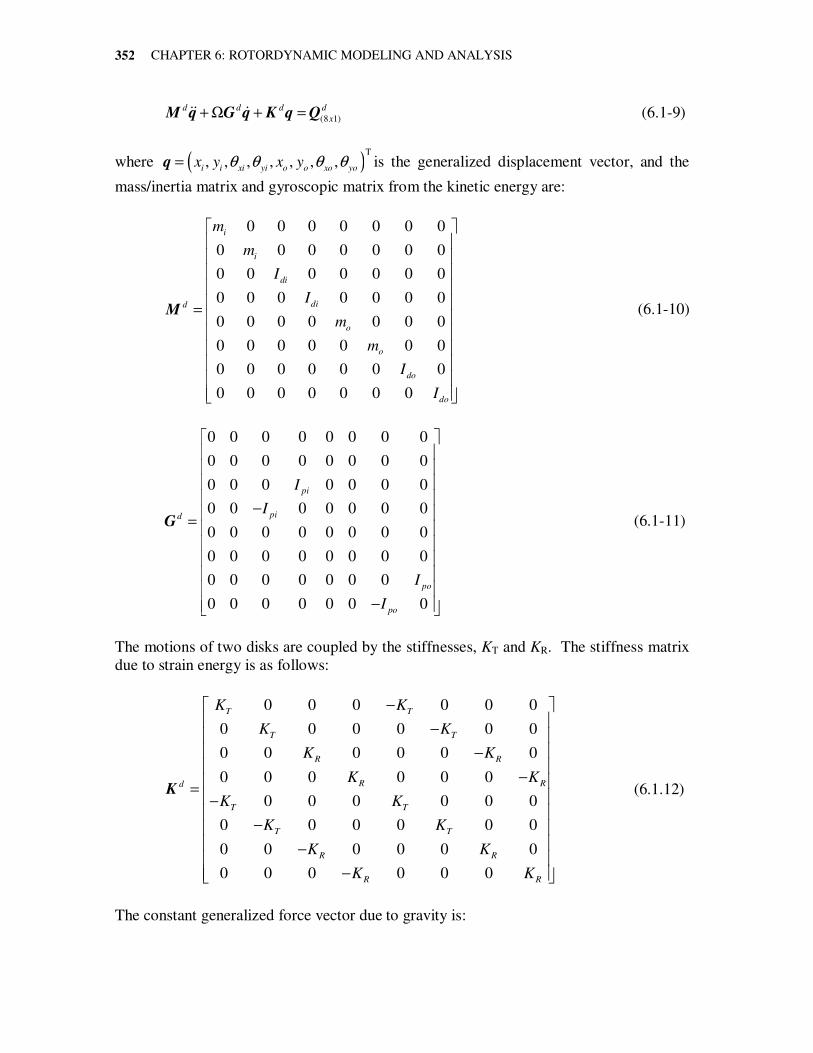
(8 1)
d d d d
x+ Ω + =M q G q K q Qɺɺ ɺ (6.1-9)
where ( )T
, , , , , , ,i i xi yi o o xo yo
x y x yθ θ θ θ=q is the generalized displacement vector, and the
mass/inertia matrix and gyroscopic matrix from the kinetic energy are:
0 0 0 0 0 0 0
0 0 0 0 0 0 0
0 0 0 0 0 0 0
0 0 0 0 0 0 0
0 0 0 0 0 0 0
0 0 0 0 0 0 0
0 0 0 0 0 0 0
0 0 0 0 0 0 0
i
i
di
did
o
o
do
do
m
m
I
I
m
m
I
I
=
M (6.1-10)
0 0 0 0 0 0 0 0
0 0 0 0 0 0 0 0
0 0 0 0 0 0 0
0 0 0 0 0 0 0
0 0 0 0 0 0 0 0
0 0 0 0 0 0 0 0
0 0 0 0 0 0 0
0 0 0 0 0 0 0
pi
pid
po
po
I
I
I
I
− =
−
G (6.1-11)
The motions of two disks are coupled by the stiffnesses, KT and KR. The stiffness matrix
due to strain energy is as follows:
0 0 0 0 0 0
0 0 0 0 0 0
0 0 0 0 0 0
0 0 0 0 0 0
0 0 0 0 0 0
0 0 0 0 0 0
0 0 0 0 0 0
0 0 0 0 0 0
T T
T T
R R
R Rd
T T
T T
R R
R R
K K
K K
K K
K K
K K
K K
K K
K K
− − −
− = −
− −
−
K (6.1.12)
The constant generalized force vector due to gravity is:
6.1 ANALYTICAL MODELS AND ESSENTIAL COMPONENTS
353
( ), , 0, 0, , , 0, 0T
d d
g i x i y o x o ym g m g m g m g= =Q M g (6.1-13)
The generalized force vector due to mass unbalance and disk skew will be discussed
later. The synchronous excitation due to the mass unbalance is the most important
excitation for a rotor system. Since the emphasis here is to study rotor dynamics, for an
integrated disk, the translational displacements of both inner and outer disks are generally
considered to be the same (xi=xo, yi=yo), that is, KT is infinitely large, and the outer disk
motion can be described by two rotational displacements to approximate the first nodal
diameter mode of the disk. The outer disk is no longer remaining normal to the shaft
during vibration, but has its own rotational motion, as illustrated in Figure 6.1-10.
Therefore, for a flexible disk used in rotordynamic study, the disk motion can usually be
described by the (6×1) generalized displacements, ( )T
, , , , ,x y xo yo
x y θ θ θ θ=q , which
contain two extra rotational DOFs for the flexible disk in addition to the original four
DOFs at the rotor station for the rigid disk.
When the translational displacements are the same for both disks, the translational
kinetic energy can be combined and is equivalent to a single mass (md=mi+mo) that acts at
the rotor station. The equation of motion for a rotating flexible disk (6 DOFs) now
becomes:
(6 1)
d d d d d d d
x+ Ω + =M q G q K q Qɺɺ ɺ (6.1-14)
where ( )T
, , , , ,x y xo yo
x y θ θ θ θ=q and ( ),xo yo
θ θ are the additional DOFs for the outer
disk. The associated mass/inertia matrix, gyroscopic matrix, stiffness matrix, and
generalized force vector due to gravity become:
0 0 0 0 0
0 0 0 0 0
0 0 0 0 0
0 0 0 0 0
0 0 0 0 0
0 0 0 0 0
d
d
did
di
do
do
m
m
I
I
I
I
=
M (6.1-15)
0 0 0 0 0 0
0 0 0 0 0 0
0 0 0 0 0
0 0 0 0 0
0 0 0 0 0
0 0 0 0 0
pid
pi
po
po
I
I
I
I
= −
−
G (6.1.16)
CHAPTER 6: ROTORDYNAMIC MODELING AND ANALYSIS
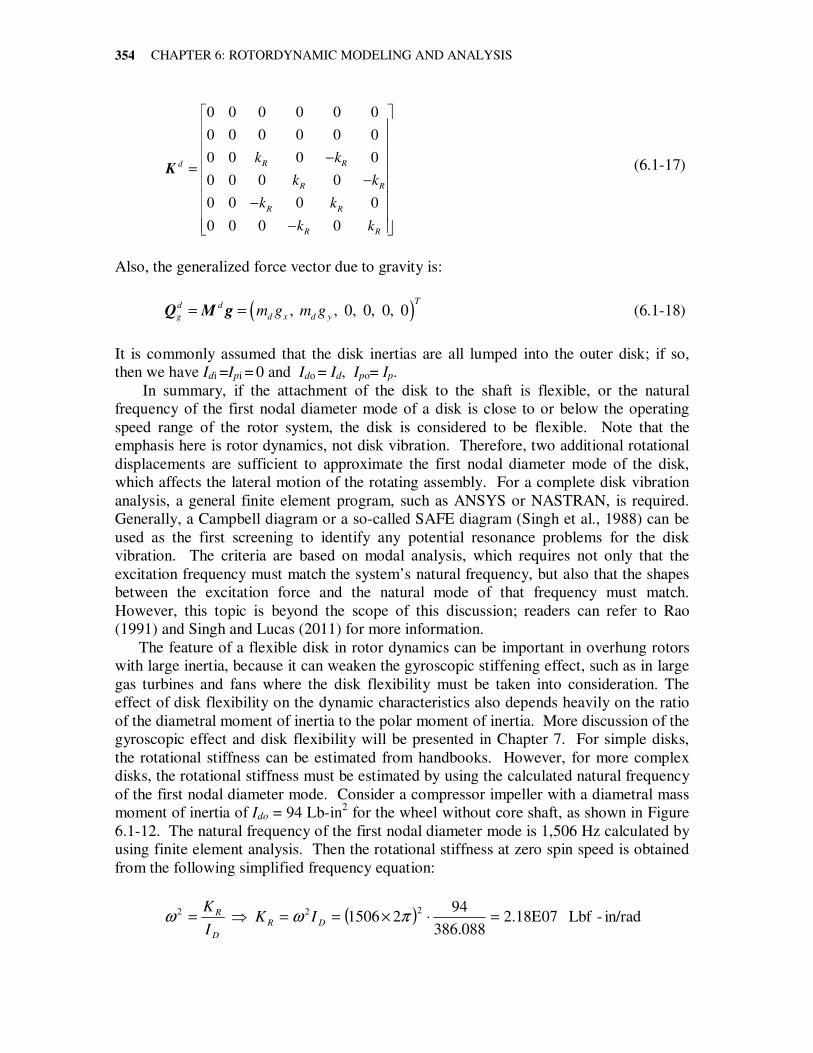
354
0 0 0 0 0 0
0 0 0 0 0 0
0 0 0 0
0 0 0 0
0 0 0 0
0 0 0 0
R Rd
R R
R R
R R
k k
k k
k k
k k
−
= −
−
−
K (6.1-17)
Also, the generalized force vector due to gravity is:
( ), , 0, 0, 0, 0T
d d
g d x d ym g m g= =Q M g (6.1-18)
It is commonly assumed that the disk inertias are all lumped into the outer disk; if so,
then we have Idi =Ipi = 0 and Ido = Id, Ipo= Ip.
In summary, if the attachment of the disk to the shaft is flexible, or the natural
frequency of the first nodal diameter mode of a disk is close to or below the operating
speed range of the rotor system, the disk is considered to be flexible. Note that the
emphasis here is rotor dynamics, not disk vibration. Therefore, two additional rotational
displacements are sufficient to approximate the first nodal diameter mode of the disk,
which affects the lateral motion of the rotating assembly. For a complete disk vibration
analysis, a general finite element program, such as ANSYS or NASTRAN, is required.
Generally, a Campbell diagram or a so-called SAFE diagram (Singh et al., 1988) can be
used as the first screening to identify any potential resonance problems for the disk
vibration. The criteria are based on modal analysis, which requires not only that the
excitation frequency must match the system’s natural frequency, but also that the shapes
between the excitation force and the natural mode of that frequency must match.
However, this topic is beyond the scope of this discussion; readers can refer to Rao
(1991) and Singh and Lucas (2011) for more information.
The feature of a flexible disk in rotor dynamics can be important in overhung rotors
with large inertia, because it can weaken the gyroscopic stiffening effect, such as in large
gas turbines and fans where the disk flexibility must be taken into consideration. The
effect of disk flexibility on the dynamic characteristics also depends heavily on the ratio
of the diametral moment of inertia to the polar moment of inertia. More discussion of the
gyroscopic effect and disk flexibility will be presented in Chapter 7. For simple disks,
the rotational stiffness can be estimated from handbooks. However, for more complex
disks, the rotational stiffness must be estimated by using the calculated natural frequency
of the first nodal diameter mode. Consider a compressor impeller with a diametral mass
moment of inertia of Ido = 94 Lb-in2 for the wheel without core shaft, as shown in Figure
6.1-12. The natural frequency of the first nodal diameter mode is 1,506 Hz calculated by
using finite element analysis. Then the rotational stiffness at zero spin speed is obtained
from the following simplified frequency equation:
( ) in/rad-Lbf 07E18.2088.386
9421506
222 =⋅×==⇒= πωω DR
D
R IKI
K
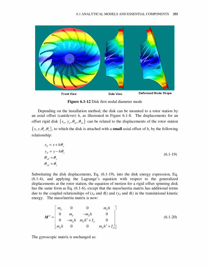
6.1 ANALYTICAL MODELS AND ESSENTIAL COMPONENTS
355
Figure 6.1-12 Disk first nodal diameter mode
Depending on the installation method, the disk can be mounted to a rotor station by
an axial offset (cantilever) h, as illustrated in Figure 6.1-8. The displacements for an
offset rigid disk ( ), , ,d d xd ydx y θ θ can be related to the displacements of the rotor station
( ), , ,x yx y θ θ , to which the disk is attached with a small axial offset of h, by the following
relationship:
yyd
xxd
xd
yd
hyy
hxx
θθ
θθ
θ
θ
=
=
−=
+=
(6.1-19)
Substituting the disk displacements, Eq. (6.1-19), into the disk energy expression, Eq.
(6.1-4), and applying the Lagrange’s equation with respect to the generalized
displacements at the rotor station, the equation of motion for a rigid offset spinning disk
has the same form as Eq. (6.1-6), except that the mass/inertia matrix has additional terms
due to the coupled relationships of (xd and θy) and (yd and θx) in the translational kinetic
energy. The mass/inertia matrix is now:
2
2
0 0
0 0
0 0
0 0
d d
d dd
d d d
d d d
m m h
m m h
m h m h I
m h m h I
− = − +
+
M (6.1-20)
The gyroscopic matrix is unchanged as:
CHAPTER 6: ROTORDYNAMIC MODELING AND ANALYSIS
356
0 0 0 0
0 0 0 0
0 0 0
0 0 0
d
p
p
I
I
=
−
G (6.1-21)
The constant generalized force vector due to gravity is given by:
x d x
y d yd d
g
x d y
y d xg
F m g
F m g
M m hg
M m hg
= = = −
Q M g (6.1-22)
For an offset flexible disk, where the flexibility occurs at the disk, the relationships of
the disk displacements ( ), , , , , , ,i i xi yi o o xo yo
x y x yθ θ θ θ and rotor displacements ( ), , ,x y
x y θ θ
are:
i o y
i o x
xi x
yi y
xo x
yo y
x x x h
y y y h
θ
θ
θ θ
θ θ
θ θ
θ θ
= = +
= = −
=
=
≠
≠
(6.1-23)
The associated modified mass matrix for this offset flexible disk becomes:
2
2
0 0 0 0
0 0 0 0
0 ( ) 0 0 0
0 0 ( ) 0 0
0 0 0 0 0
0 0 0 0 0
d d
d d
d d did
d d di
do
do
m m h
m m h
m h m h I
m h m h I
I
I
− − +
= +
M (6.1-24)
The associated gyroscopic and stiffness matrices are the same as Eqs. (6.1-16) and (6.1-
17). Note that this offset must be small enough for the linear assumption to be valid. For
a large offset, the linear relationships between the displacements of the shaft and disk no
longer apply. The disk must be considered and modeled separately.
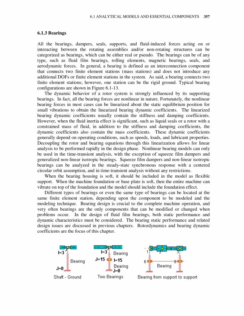
6.1 ANALYTICAL MODELS AND ESSENTIAL COMPONENTS
357
6.1.3 Bearings
All the bearings, dampers, seals, supports, and fluid-induced forces acting on or
interacting between the rotating assemblies and/or non-rotating structures can be
categorized as bearings, which can be either real or pseudo. The bearings can be of any
type, such as fluid film bearings, rolling elements, magnetic bearings, seals, and
aerodynamic forces. In general, a bearing is defined as an interconnection component
that connects two finite element stations (mass stations) and does not introduce any
additional DOFs or finite element stations in the system. As said, a bearing connects two
finite element stations; however, one station can be the rigid ground. Typical bearing
configurations are shown in Figure 6.1-13.
The dynamic behavior of a rotor system is strongly influenced by its supporting
bearings. In fact, all the bearing forces are nonlinear in nature. Fortunately, the nonlinear
bearing forces in most cases can be linearized about the static equilibrium position for
small vibrations to obtain the linearized bearing dynamic coefficients. The linearized
bearing dynamic coefficients usually contain the stiffness and damping coefficients.
However, when the fluid inertia effect is significant, such as liquid seals or a rotor with a
constrained mass of fluid, in addition to the stiffness and damping coefficients, the
dynamic coefficients also contain the mass coefficients. These dynamic coefficients
generally depend on operating conditions, such as speeds, loads, and lubricant properties.
Decoupling the rotor and bearing equations through this linearization allows for linear
analysis to be performed rapidly in the design phase. Nonlinear bearing models can only
be used in the time-transient analysis, with the exception of squeeze film dampers and
generalized non-linear isotropic bearings. Squeeze film dampers and non-linear isotropic
bearings can be analyzed in the steady-state synchronous response with a centered
circular orbit assumption, and in time-transient analysis without any restrictions.
When the bearing housing is soft, it should be included in the model as flexible
support. When the machine foundation or base plate is soft, then the entire machine can
vibrate on top of the foundation and the model should include the foundation effect.
Different types of bearings or even the same type of bearings can be located at the
same finite element station, depending upon the component to be modeled and the
modeling technique. Bearing design is crucial to the complete machine operation, and
very often bearings are the only components that can be modified or changed when
problems occur. In the design of fluid film bearings, both static performance and
dynamic characteristics must be considered. The bearing static performance and related
design issues are discussed in previous chapters. Rotordynamics and bearing dynamic
coefficients are the focus of this chapter.
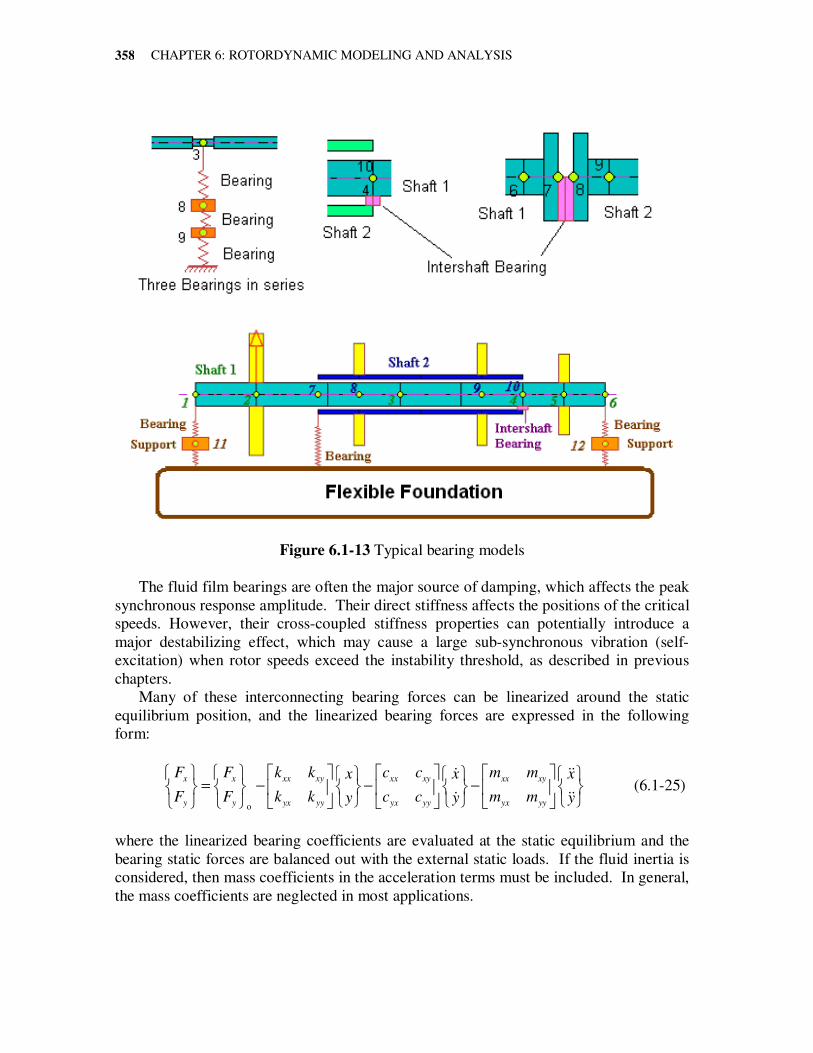
CHAPTER 6: ROTORDYNAMIC MODELING AND ANALYSIS
358
Figure 6.1-13 Typical bearing models
The fluid film bearings are often the major source of damping, which affects the peak
synchronous response amplitude. Their direct stiffness affects the positions of the critical
speeds. However, their cross-coupled stiffness properties can potentially introduce a
major destabilizing effect, which may cause a large sub-synchronous vibration (self-
excitation) when rotor speeds exceed the instability threshold, as described in previous
chapters.
Many of these interconnecting bearing forces can be linearized around the static
equilibrium position, and the linearized bearing forces are expressed in the following
form:
o
x x xx xy xx xy xx xy
y y yx yy yx yy yx yy
F F k k c c m mx x x
F F k k c c m my y y
= − − −
ɺ ɺɺ
ɺ ɺɺ (6.1-25)
where the linearized bearing coefficients are evaluated at the static equilibrium and the
bearing static forces are balanced out with the external static loads. If the fluid inertia is
considered, then mass coefficients in the acceleration terms must be included. In general,
the mass coefficients are neglected in most applications.
6.1 ANALYTICAL MODELS AND ESSENTIAL COMPONENTS
359
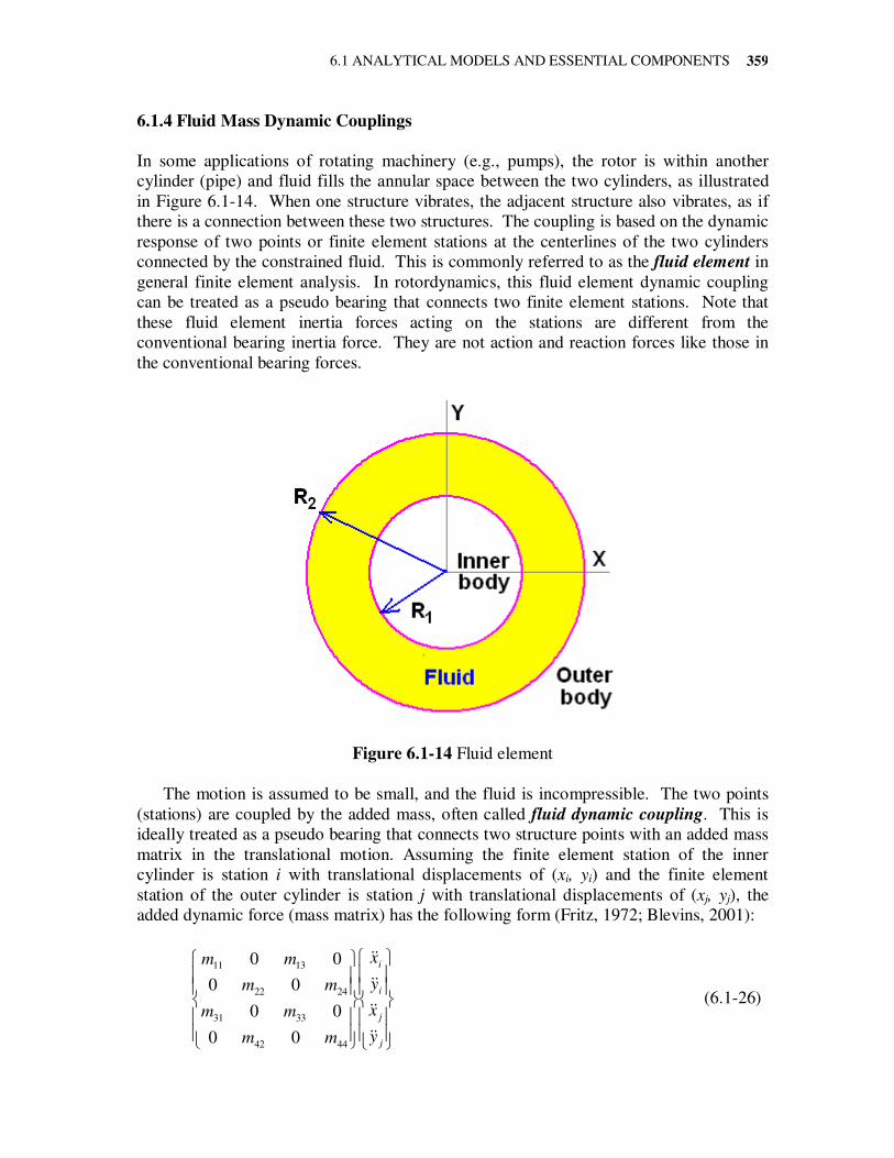
6.1.4 Fluid Mass Dynamic Couplings
In some applications of rotating machinery (e.g., pumps), the rotor is within another
cylinder (pipe) and fluid fills the annular space between the two cylinders, as illustrated
in Figure 6.1-14. When one structure vibrates, the adjacent structure also vibrates, as if
there is a connection between these two structures. The coupling is based on the dynamic
response of two points or finite element stations at the centerlines of the two cylinders
connected by the constrained fluid. This is commonly referred to as the fluid element in
general finite element analysis. In rotordynamics, this fluid element dynamic coupling
can be treated as a pseudo bearing that connects two finite element stations. Note that
these fluid element inertia forces acting on the stations are different from the
conventional bearing inertia force. They are not action and reaction forces like those in
the conventional bearing forces.
Figure 6.1-14 Fluid element
The motion is assumed to be small, and the fluid is incompressible. The two points
(stations) are coupled by the added mass, often called fluid dynamic coupling. This is
ideally treated as a pseudo bearing that connects two structure points with an added mass
matrix in the translational motion. Assuming the finite element station of the inner
cylinder is station i with translational displacements of (xi, yi) and the finite element
station of the outer cylinder is station j with translational displacements of (xj, yj), the
added dynamic force (mass matrix) has the following form (Fritz, 1972; Blevins, 2001):
j
j
i
i
y
x
y
x
mm
mm
mm
mm
ɺɺ
ɺɺ
ɺɺ
ɺɺ
4442
3331
2422
1311
00
00
00
00
(6.1-26)
CHAPTER 6: ROTORDYNAMIC MODELING AND ANALYSIS
360
Assume that the inner cylinder has an outer radius of R1 and the outer cylinder has an
inner radius of R2. The length of the cylinder is L, and the density of the fluid is ρ. The
values for the mass coefficients are:
2 2
2 2 111 22 1 2 2
2 1
R R
m m LRR R
ρπ +
= = −
= added mass of inner cylinder (6.1-27)
2 2
2 2 133 44 2 2 2
2 1
R R
m m LRR R
ρπ +
= = −
= added mass of outer cylinder (6.1-28)
2 2
1 213 31 24 42 2 2
2 1
2R Rm m m m L
R Rρπ
= = = = −
− = fluid coupling (6.1-29)
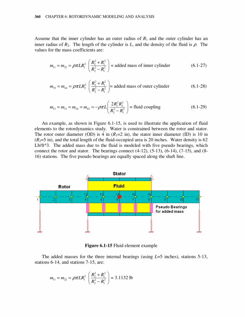
An example, as shown in Figure 6.1-15, is used to illustrate the application of fluid
elements to the rotordynamics study. Water is constrained between the rotor and stator.
The rotor outer diameter (OD) is 4 in (R1=2 in), the stator inner diameter (ID) is 10 in
(R2=5 in), and the total length of the fluid-occupied area is 20 inches. Water density is 62
Lb/ft^3. The added mass due to the fluid is modeled with five pseudo bearings, which
connect the rotor and stator. The bearings connect (4-12), (5-13), (6-14), (7-15), and (8-
16) stations. The five pseudo bearings are equally spaced along the shaft line.
Figure 6.1-15 Fluid element example
The added masses for the three internal bearings (using L=5 inches), stations 5-13,
stations 6-14, and stations 7-15, are:
2 2
2 2 111 22 1 2 2
2 1
R R
m m LRR R
ρπ +
= = −
= 3.1132 lb
6.1 ANALYTICAL MODELS AND ESSENTIAL COMPONENTS
361
2 2
2 2 133 44 2 2 2
2 1
R R
m m LRR R
ρπ +
= = −
= 19.4575 lb
2 2
1 213 31 24 42 2 2
2 1
2R Rm m m m L
R Rρπ
= = = = −
− = −5.3676 lb
The added masses for bearings at both ends of the fluid element (using L=2.5 inches,
which is half the distance between two pseudo bearings), stations 4-12 and stations 8-16,
are:
2 2
2 2 111 22 1 2 2
2 1
R R
m m LRR R
ρπ +
= = −
= 1.5566 lb
2 2
2 2 133 44 2 2 2
2 1
R R
m m LRR R
ρπ +
= = −
= 9.7287 lb
2 2
1 213 31 24 42 2 2
2 1
2R Rm m m m L
R Rρπ
= = = = −
− = −2.6838 lb
6.1.5 Flexible Foundation and Supports
If a flexible foundation and/or flexible supports are present, the equation of motion for
this non-rotating structure under the small vibration assumption is as follows:
)()( )( )( tttt fff QqKqCqM =++ ɺɺɺ (6.1-30)
Again, the mass/inertia matrix Mf is a positive definite real symmetric matrix. The
restrained structural stiffness matrix Kf is also a positive definite real symmetric matrix.
For practical purposes, the damping properties of the foundation structure are seldom
known in the same way as the inertia and stiffness properties, so it is not feasible to
construct the damping matrix analogous to the construction of the mass/inertia and
stiffness matrices. Also, the damping for the foundation structure is extremely small and
usually neglected in the modeling for rotordynamic study. If necessary, Rayleigh
damping is commonly employed in the foundation structure to define the damping
matrix. The simplest procedure for defining a foundation structural damping matrix is
so-called proportional damping, as follows:
fff KMC βα += (6.1-31)
CHAPTER 6: ROTORDYNAMIC MODELING AND ANALYSIS
362
where α and β are two constants chosen to produce desirable modal damping factors for
two selected modes. Once α and β are given, the damping matrix is determined and the
damping factors in the remaining modes are then determined by the orthogonality
relationship:
+= i
i
i βωω
αξ
2
1 i=1, 2,….., N (6.1-32)
where iξ is the modal damping factor and iω is the ith undamped natural frequency
obtained from the foundation structure eigenvalue problem:
( ) 0φMK =− ifif 2ω i=1, 2,….., N (6.1-33)
whereiφ is the associated ith eigenvector. N is the number of DOFs for the foundation
(support) structure. The drawback of the above proportional damping method is that it is
limited to two damping factors, and others are determined accordingly by Eq. (6.1-32),
which may not be realistic for other modes of interest. A more generalized approach is
by specifying the damping factors for all the modes of interest and utilizing the
orthogonality relationship; the physical damping matrix can then be constructed as
follows:
( )( )Tifif
NN
i i
ii
fM
φMφMC 2
ˆ
1
∑<<
=
=
ωξ (6.1-34)
where the modal mass for the ith mode Mi is defined as:
iif
T
i M=φMφ (6.1-35)
and the number of retained (interested) modes N is far less than the total number of
modes N in practice. The damping matrix defined by the above approaches is a real
symmetric matrix, which is known as Rayleigh’s dissipative damping matrix. Again, all
the matrices in the foundation structure are real symmetric and generally independent of
the rotor speed.
6.1.6 Excitations
Mass unbalance is the most common source of synchronous excitation in rotating
machinery. The rotors always have some amount of residual unbalance, no matter how
well they are balanced and assembled. The unbalance excitation is a harmonic
synchronous excitation, which has an excitation frequency equal to the rotor rotational
frequency (1×Ω). The mass unbalance excitation magnitude varies with the square of the
rotor speed (meΩ2), where m is the mass, e is the mass eccentricity, and Ω is the rotor
rotational speed in rad/sec. There are other sources of synchronous excitation, such as
6.1 ANALYTICAL MODELS AND ESSENTIAL COMPONENTS
363
excitations due to disk skew, shaft bow, coupling misalignment, and magnetic forces.
The disk skew excitation moments ( )( )2 Ω− τdp II due to the skew angle of τ are similar
to the unbalance forces associated with mass eccentricity e. Both excitation magnitudes
are functions of the square of the rotor speed, and the excitation frequencies are
synchronous with the rotor speed. Disk skew produces an external moment, but mass
eccentricity produces an external force. The residual shaft bow can be present in the
large rotor systems for many reasons, including assembly tolerances and uneven thermal
distribution. When a residual shaft bow exists in a rotor system, a constant magnitude
rotating force ( bsqK ), which is synchronized with the shaft spin speed, is acting on the
rotor system. The shaft bow rotates with the rotating reference frame; therefore, it is
commonly specified in the rotating reference coordinate system. Coupling misalignment
and magnetic forces are similar to the shaft bow excitation with a constant magnitude
rotating force.
Other types of excitations and loadings exist in rotor-bearing systems. Some are
constant, such as static and gravity loads, some are frequency and/or speed related, and
some are time-dependent transient excitations. Time-transient analysis may be required
when these excitations are considered. Commonly, constant static loads are used in the
bearing linearization process and are canceled out in the linear equation of motion.
6.1.7 System Equations of Motion and Analyses
The system governing equations of motion for a complete rotor-bearing-support
(foundation) system are obtained by assembling the equations of motion of all the
components. The assembled system equations of motions with a constant rotational speed
Ω are:
( ) ( ) ),,()( )( )( ttttt nb qqQQqKqGCqM ɺɺɺɺ +=+Ω++ (6.1-36)
where all the matrices are real and assembled from the associated components. The
generalized coordinate vector q is the system displacement vector to be solved. The
mass/inertia matrix M is a positive definite real symmetric matrix. In rotordynamics, the
mass/inertia matrix is derived from the kinetic energy; it is said to be nonsingular and its
determinant is not zero. The gyroscopic matrix ΩG is a real skew-symmetric matrix
derived from the conservative gyroscopic forces of the rotating components. Although
the gyroscopic matrix is linear in generalized velocity coordinates, it is conservative in
nature. The damping matrix C contains the linearized bearing/support damping matrix
bC , which can be a real arbitrary matrix, and the dissipative matrix from foundation fC ,
if included, which is a real symmetric matrix. For systems with linearized fluid film
bearings without fluid inertia effects, bC is a real symmetric matrix. The dissipative
damping force is non-conservative and removes energy from the system, which stabilizes
the system. The stiffness matrix K contains the conservative elastic real symmetric
matrices from the rotating components and flexible foundation, if the foundation is
included, and also the non-conservative linearized bearing/support stiffness matrix bK ,
which is a real arbitrary matrix in general. The unequal cross-coupled stiffness from the
CHAPTER 6: ROTORDYNAMIC MODELING AND ANALYSIS
364
fluid film bearings forms the circulatory matrix, which can add energy to the system and
have a destabilizing effect, as discussed in Chapter 2. The stiffness matrix can also
contain the contribution from the gravity moments for vertical rotor systems, which is a
real non-symmetric matrix and can affect both the critical speeds and rotor stability. The
topic of vertical rotors will be discussed in Chapter 7. The forcing vector ( )tQ contains
all the time-dependent excitations, which are independent of the generalized coordinates.
The force vector ),,( tnb qqQ ɺ contains all other forces including constant, linear, and
nonlinear forces. For linear bearings, lb
= − −b bQ C q K qɺ , where bC and bK can be
placed in the left-hand side of the equation.
As described earlier, any real matrix can be written as a sum of a symmetric matrix
and a skew-symmetric matrix, so Eq. (6.1-36) can be re-organized as a more known
general dynamic system equation of motion (Meirovitch, 1980):
( ) ( ) ( )* ( ) ( ) ( ) ( , , )s nbt t t t t+ + + + = +M q D G q K H q Q Q q qɺɺ ɺ ɺ (6.1-37)
where all the matrices are real, M (mass/inertia matrix), D (damping matrix), and Ks
(stiffness matrix) being symmetric, and G* (gyroscopic matrix with spin speed) and H
(circulatory matrix) being skew-symmetric. Two unique matrices are present in the
rotordynamics study: the conservative gyroscopic matrix G* caused by the rotor spinning
effect and the non-conservative circulatory matrix H caused by the cross-coupled
stiffness coefficients from bearings, seals, fluid interactions, and gravity moments for
vertical rotors. The gyroscopic effect couples two planes of motion (X-Z and Y-Z planes
with the Z-axis being the spinning axis) and splits the planar mode into two precessional
modes: one with forward precession and the other with backward precession. As the
speed increases, the forward whirl frequencies increase and the backward whirl
frequencies decrease if only the purely gyroscopic effect is considered in the system.
This is known as the gyroscopic stiffening effect on forward precessional modes and the
softening effect on backward precessional modes. The kinetic energy due to the
gyroscopic moments is linearly proportional to the rotor spin speed, whirl frequency,
polar moment of inertia, and area of rotational displacement (slope) orbit. Therefore, the
gyroscopic effect has greater influence for higher rotor speeds, vibratory modes with
higher frequencies and large rotational displacements (slopes). However, the gyroscopic
moment is a conservative force which has no influence on the system stability study. On
the other hand, the non-conservative cross-coupled stiffness coefficients (kxy and kyx)
caused by fluid film bearings, seals, and other fluid interactions, such as aerodynamic
cross-coupling, may produce a major destabilizing effect on the rotor system. This
destabilizing effect may cause the rotor system to be in a very destructive, self-excited
state. In general, the cross-coupled stiffness has little influence on the system natural
frequencies, unless its value becomes very large.
In some applications, it is necessary to study the rotor transient motion during startup,
shutdown, movement through critical speeds, and rotor drop for magnetic bearing
systems. In these situations, the angular velocity (spin speed) is no longer a constant, but
is a function of time. The governing equations of motion for a variable rotational speed
system are (Chen & Gunter, 2005):
6.1 ANALYTICAL MODELS AND ESSENTIAL COMPONENTS
365
[ ] [ ]
( ) ( ) ( )t
ttt
nl ,,,,,
)( )( )(
21
2 ϕϕϕϕϕϕϕ
ϕϕ
ɺɺɺɺɺɺɺ
ɺɺɺɺɺɺ
qqQQQ
qGKqGCqM
++=
++++ (6.1-38)
and subject to the initial conditions:
( ) ( ) 0 ,0 oo qqqq ɺɺ == (6.1-39)
where ϕϕϕ ɺɺɺ and , , are the angular displacement, angular velocity ( Ω=ϕɺ ), and angular
acceleration (deceleration) of the rotor system. Two additional terms introduced in the
governing equations due to the speed variation are circulatory matrix ϕGɺɺ and forcing
vector 2Qϕɺɺ . The equations of motion for a variable rotational speed system, Eq. (6.1-38),
are nonlinear and can only be analyzed using time-transient analysis.
All rotating systems are nonlinear. In rotordynamics, the rotor vibration is very small
compared to the shaft dimensions, the small shaft deformation assumption is justifiable,
and the equations of motion for the rotating structural components are linear. However,
the bearing forces can be highly nonlinear. In general, for small vibrations and rotor
speeds below the instability threshold, the rotor dynamic behaviors predicted by using
linear analyses with linearized bearing dynamic coefficients provide reasonable results.
For large vibrations or rotor speeds beyond the instability threshold, linear theory is no
longer valid, and nonlinear analysis is needed. For systems with highly nonlinear
bearings/dampers in which linearization is not feasible, nonlinear analyses are required.
Most rotordynamic solution techniques are for linear systems based on linear theory,
such as critical speed analysis, whirl speed/stability analysis, and steady-state harmonic
response analysis. They provide sound engineering information for system design
purposes. For systems in which linearization is not feasible, such as squeeze film
dampers, and systems in which the rotor speeds exceed the instability threshold
established by the linear whirl speed and stability analysis, nonlinear analyses are
required. Two nonlinear analyses in rotordynamics are time-transient analysis using
numerical integration and steady-state response analysis using harmonic balancing or
trigonometric collocation methods. Since time-transient analysis provides transient and
steady-state response and is a more straight forward technique than the harmonic
balancing and trigonometric collocation methods; therefore, almost all nonlinear systems
are analyzed using time-transient analysis nowadays due to high-speed computational
power. Time-transient analysis can also be used for linear systems.
The most common analyses performed during the design of rotor-bearing systems
are:
• Static deflection and bearing loads due to gravity, static loads, misalignments,
and any other constant forces and constraints. This also includes the so-called
catenary curve analysis for larger turbo-generator systems. The system analyzed
is a linear system.
• Steady maneuver response and bearing loads due to constant base translational
acceleration or turn rate, which is commonly analyzed in aerospace applications.
The system analyzed is a linear system.
• Critical speed analysis, mode shapes and energy distribution. The system
analyzed is a linear, isotropic, and undamped system with constant and speed-
CHAPTER 6: ROTORDYNAMIC MODELING AND ANALYSIS
366
independent bearing/support stiffness. The analysis provides estimated critical
speeds for design purposes.
• Critical speed map. This is used to facilitate shaft design and preliminary
bearing design. This map is an outgrowth of the critical speed analysis by
assuming the bearing stiffness in a range from soft to rigid. In this analysis, the
actual bearing properties are not known and the design range for the bearing
stiffness is to be determined from this map. The bearing dynamic stiffness is
often overlapped in the map to estimate the critical speeds.
• Steady-state synchronous response and transmitted loads due to mass
unbalance, disk skew, and shaft bow. The system analyzed can be either linear or
nonlinear. For a nonlinear system, isotropic properties and centered circular
orbits are assumed.
• Steady-state response due to non-synchronous harmonic excitations. This is
for linear systems only.
• Whirl speed and stability analysis, damped natural frequencies of whirl,
logarithmic decrements or damping factors, and associated mode shapes. The
system analyzed is a linear system. The system’s stability and instability threshold
can be established. For systems with negative logarithmic decrements, linear
theory is no longer valid and nonlinear time-transient analysis is required.
• Time-transient analysis. The system analyzed can be linear or nonlinear at a
constant rotor speed or during startup and shutdown.
6.2 Modeling Considerations
When building the rotor model, one must know the purposes of analyzing it. Is it a
general finite element analysis, such as stress/strain analysis due to centrifugal force and
pressure distribution, thermal analysis, or impeller blade vibration? Or is it a
rotordynamics analysis, such as critical speed analysis, rotor stability analysis, or rotor
response analysis? The purpose of modeling is to convert the actual continuous system
into a discrete mathematical model and develop physical insights into the actual system
to facilitate the design process. For rotordynamics analysis, there are some basic
principles and concepts to follow:
1. Rotor modeling is not an exact science. Assumptions and simplifications are
needed for design purposes and parametric study.
2. Use the simplest model possible as long as it contains all the necessary
information and is a good representation of the system. Do not over-model the
system, which may complicate comprehension of the analysis results and does not
necessarily provide more accurate results due to potential modeling errors.
3. Practical experience and engineering judgment must be applied during the
modeling process.
4. The manufacturing and assembly tolerance must be considered.
5. The variations in the operating conditions must be considered.
6.2 MODELING CONSIDERATIONS
367
6. Use known information and test data to refine and verify the model if they are
available, such as the total weight, center of gravity (CG) location, bearing
locations, free-free modal frequency, and any other test data.
The most common questions raised in modeling the rotor shaft are: (1) How many
elements (or finite element stations) are required to accurately predict the dynamic
behavior of the system? and (2) How should we select the station’s locations? To answer
these questions, let us first examine a simple rotor system, as shown in Figure 6.2-1.
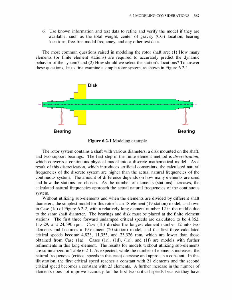
Figure 6.2-1 Modeling example
The rotor system contains a shaft with various diameters, a disk mounted on the shaft,
and two support bearings. The first step in the finite element method is discretization,
which converts a continuous physical model into a discrete mathematical model. As a
result of this discretization, which introduces artificial constraints, the calculated natural
frequencies of the discrete system are higher than the actual natural frequencies of the
continuous system. The amount of difference depends on how many elements are used
and how the stations are chosen. As the number of elements (stations) increases, the
calculated natural frequencies approach the actual natural frequencies of the continuous
system.
Without utilizing sub-elements and when the elements are divided by different shaft
diameters, the simplest model for this rotor is an 18-element (19-station) model, as shown
in Case (1a) of Figure 6.2-2, with a relatively long element number 12 in the middle due
to the same shaft diameter. The bearings and disk must be placed at the finite element
stations. The first three forward undamped critical speeds are calculated to be 4,862,
11,629, and 24,590 rpm. Case (1b) divides the longest element number 12 into two
elements and becomes a 19-element (20-station) model, and the first three calculated
critical speeds become 4,823, 11,355, and 23,326 rpm, which are lower than those
obtained from Case (1a). Cases (1c), (1d), (1e), and (1f) are models with further
refinements in this long element. The results for models without utilizing sub-elements
are summarized in Table 6.2-1. As expected, while the number of elements increases, the
natural frequencies (critical speeds in this case) decrease and approach a constant. In this
illustration, the first critical speed reaches a constant with 21 elements and the second
critical speed becomes a constant with 23 elements. A further increase in the number of
elements does not improve accuracy for the first two critical speeds because they have
CHAPTER 6: ROTORDYNAMIC MODELING AND ANALYSIS
368
reached a constant already, but it improves the accuracy of higher critical speeds.
However, the increase in the number of elements requires more modeling effort and
computational time.
Case 1 – without sub-elements Case 2 – with sub-elements
Figure 6.2-2 Discretization of the rotor – without and with sub-elements
Table 1.8-1 First three forward undamped critical speeds for the rotor models
without sub-elements
Without sub-elements ω1 ω2 ω3
Case (1a): 18 elements 4,862 11,629 24,590
Case (1b): 19 elements 4,823 11,355 23,326
Case (1c): 20 elements 4,821 11,332 23,225
Case (1d): 21 elements 4,820 11,326 23,190
Case (1e): 22 elements 4,820 11,324 23,177
Case (1f): 23 elements 4,820 11,323 23,170
6.2 MODELING CONSIDERATIONS
369
Without employing sub-elements in the model, each element length can be quite
different. Some elements are relatively short or long compared to others, and the
minimum number of required stations is 19 due to the geometric requirements. By
utilizing the sub-elements, the simplest model is a 4-element (5-station) model, as shown
in Case (2a) of Figure 6.2-2, where only the necessary stations (bearings, disk, and both
end-points) are kept, and others are modeled as sub-elements. Further division in the
long element is performed similar to Case (1). The results for models with sub-elements
are summarized in Table 6.2-2. Again, while the number of elements increases, the
natural frequencies decrease and approach a constant. The results also show that by
properly selecting the locations of the finite element stations and utilizing the sub-
elements, a 6-element (7-station) model with sub-elements can be as accurate as the 20-
element (21-station) model without sub-elements in terms of the first two critical speeds.
This indicates that the quality of the elements/stations is more important than the quantity of the elements/stations. As a general rule, it is recommended that the finite
element stations be equally spaced along the rotor. Also, more stations are needed at
locations where large displacements are expected. The more elements are used, the better
the results will be. The appropriate number of finite element stations (elements) depends
on the number of vibration modes of interest and the configuration of the rotor systems,
such as the number of disks, and bearings. Practical examples will be used to illustrate
the selection of finite element stations. In the finite element method, the element length-
diameter ratio and the element length are not as critical as those in the transfer matrix
method.
Table 6.2-2 First three forward undamped critical speeds for the rotor models
with sub-elements
With sub-elements ω1 ω2 ω3
Case (2a): 4 elements 4,909 12,466 24,753
Case (2b): 5 elements 4,825 11,436 23,716
Case (2c): 6 elements 4,821 11,358 23,459
Case (2d): 7 elements 4,820 11,336 23,326
Case (2e): 8 elements 4,820 11,328 23,221
Case (2f): 9 elements 4,820 11,326 23,206
In summary, the steps to build a rotor model are as follows:
1. Identify the disks, bearings, seals, probes, and other critical locations where either
the dynamic properties are known or the responses are critical to the machine.
These locations must be assigned as stations. Some seals, such as the seals in
standard industrial air compressors and blowers, are not crucial to the rotor
dynamics and their effects can be neglected. Other seals, such as the seals in
pumps and high pressure seals, can significantly affect the rotor dynamics and
their effects must be included in the model.
2. The finite element stations are recommended to be approximately equally spaced
along the rotor line for better representation of the vibration mode shapes.
CHAPTER 6: ROTORDYNAMIC MODELING AND ANALYSIS
370
3. There is no need to use a large number of stations in the model. The use of sub-
elements is strongly recommended to increase modeling flexibility for design
changes without affecting the entire model and station numbers, and to improve
the computational efficiency.
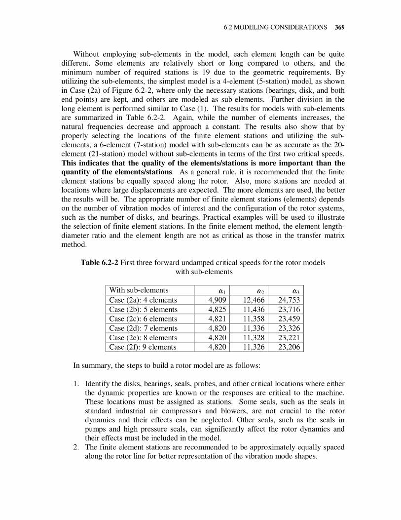
Figure 6.2-3 shows an 11-station model of a double-overhung rotor for a centrifugal
compressor. Typically, the impeller mass properties are known and lumped at the CG
location (stations 2 and 10). The aerodynamic induced cross-coupled stiffness is also
applied at the impeller CG location. Stations 4 and 8 are the stations between bearing
and vibration probe, and they are used to produce approximately equally spaced elements
and to avoid a long element. In general, this type of rotor is operated below or a little
above the free-free bending mode; hence, only the first three critical speeds are of
interest. For an 11-station model, the total DOF for lateral vibration is 44. Therefore, the
model can produce very reasonable results for the modes of interest.
Figure 6.2-3 A typical double overhung rotor model
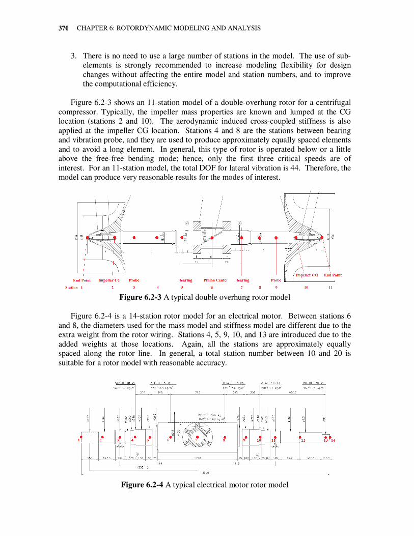
Figure 6.2-4 is a 14-station rotor model for an electrical motor. Between stations 6
and 8, the diameters used for the mass model and stiffness model are different due to the
extra weight from the rotor wiring. Stations 4, 5, 9, 10, and 13 are introduced due to the
added weights at those locations. Again, all the stations are approximately equally
spaced along the rotor line. In general, a total station number between 10 and 20 is
suitable for a rotor model with reasonable accuracy.
Figure 6.2-4 A typical electrical motor rotor model
6.2 MODELING CONSIDERATIONS
371
6.2.1 Common Modeling Mistakes
The most common mistake made in the rotor model which causes the analysis to fail or
produces incorrect results is singularity in the mass/inertia matrix. The mass/inertia
matrix is derived from the kinetic energy expression. Hence, it must be a positive definite
real matrix. This implies that for every finite element station, there should be some
mass/inertia present to produce a positive definite real matrix (i.e., positive kinetic
energy). Therefore, one should examine every finite element station to be certain that
mass is contributed either by shaft elements with positive mass density or a disk with
positive mass for the translational motions and diametral moment of inertia for the
rotational motions, if the dynamic analysis could not be performed and numerical errors
occurred.
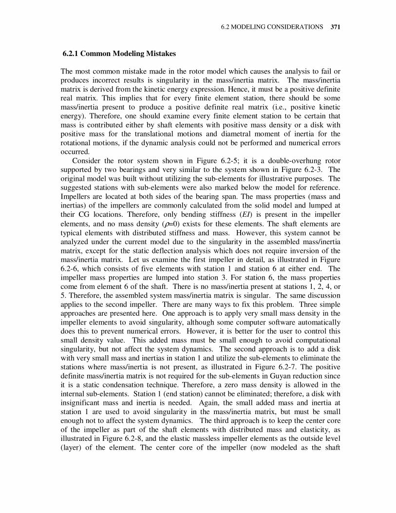
Consider the rotor system shown in Figure 6.2-5; it is a double-overhung rotor
supported by two bearings and very similar to the system shown in Figure 6.2-3. The
original model was built without utilizing the sub-elements for illustrative purposes. The
suggested stations with sub-elements were also marked below the model for reference.
Impellers are located at both sides of the bearing span. The mass properties (mass and
inertias) of the impellers are commonly calculated from the solid model and lumped at
their CG locations. Therefore, only bending stiffness (EI) is present in the impeller
elements, and no mass density (ρ=0) exists for these elements. The shaft elements are
typical elements with distributed stiffness and mass. However, this system cannot be
analyzed under the current model due to the singularity in the assembled mass/inertia
matrix, except for the static deflection analysis which does not require inversion of the
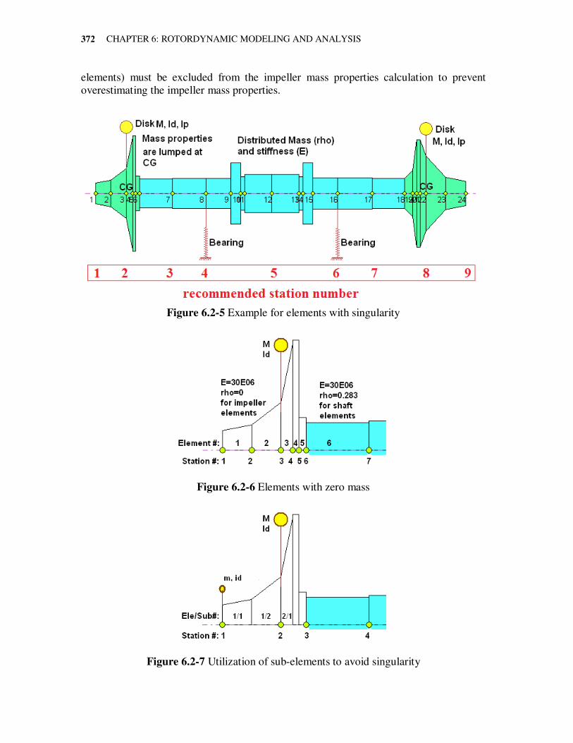
mass/inertia matrix. Let us examine the first impeller in detail, as illustrated in Figure
6.2-6, which consists of five elements with station 1 and station 6 at either end. The
impeller mass properties are lumped into station 3. For station 6, the mass properties
come from element 6 of the shaft. There is no mass/inertia present at stations 1, 2, 4, or
5. Therefore, the assembled system mass/inertia matrix is singular. The same discussion
applies to the second impeller. There are many ways to fix this problem. Three simple
approaches are presented here. One approach is to apply very small mass density in the
impeller elements to avoid singularity, although some computer software automatically
does this to prevent numerical errors. However, it is better for the user to control this
small density value. This added mass must be small enough to avoid computational
singularity, but not affect the system dynamics. The second approach is to add a disk
with very small mass and inertias in station 1 and utilize the sub-elements to eliminate the
stations where mass/inertia is not present, as illustrated in Figure 6.2-7. The positive
definite mass/inertia matrix is not required for the sub-elements in Guyan reduction since
it is a static condensation technique. Therefore, a zero mass density is allowed in the
internal sub-elements. Station 1 (end station) cannot be eliminated; therefore, a disk with
insignificant mass and inertia is needed. Again, the small added mass and inertia at
station 1 are used to avoid singularity in the mass/inertia matrix, but must be small
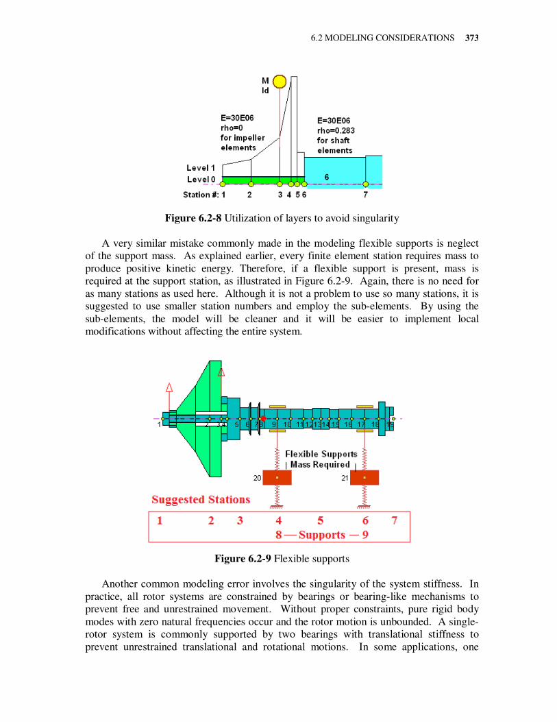
enough not to affect the system dynamics. The third approach is to keep the center core
of the impeller as part of the shaft elements with distributed mass and elasticity, as
illustrated in Figure 6.2-8, and the elastic massless impeller elements as the outside level
(layer) of the element. The center core of the impeller (now modeled as the shaft
CHAPTER 6: ROTORDYNAMIC MODELING AND ANALYSIS
372
elements) must be excluded from the impeller mass properties calculation to prevent
overestimating the impeller mass properties.
Figure 6.2-5 Example for elements with singularity
Figure 6.2-6 Elements with zero mass
Figure 6.2-7 Utilization of sub-elements to avoid singularity
6.2 MODELING CONSIDERATIONS
373
Figure 6.2-8 Utilization of layers to avoid singularity
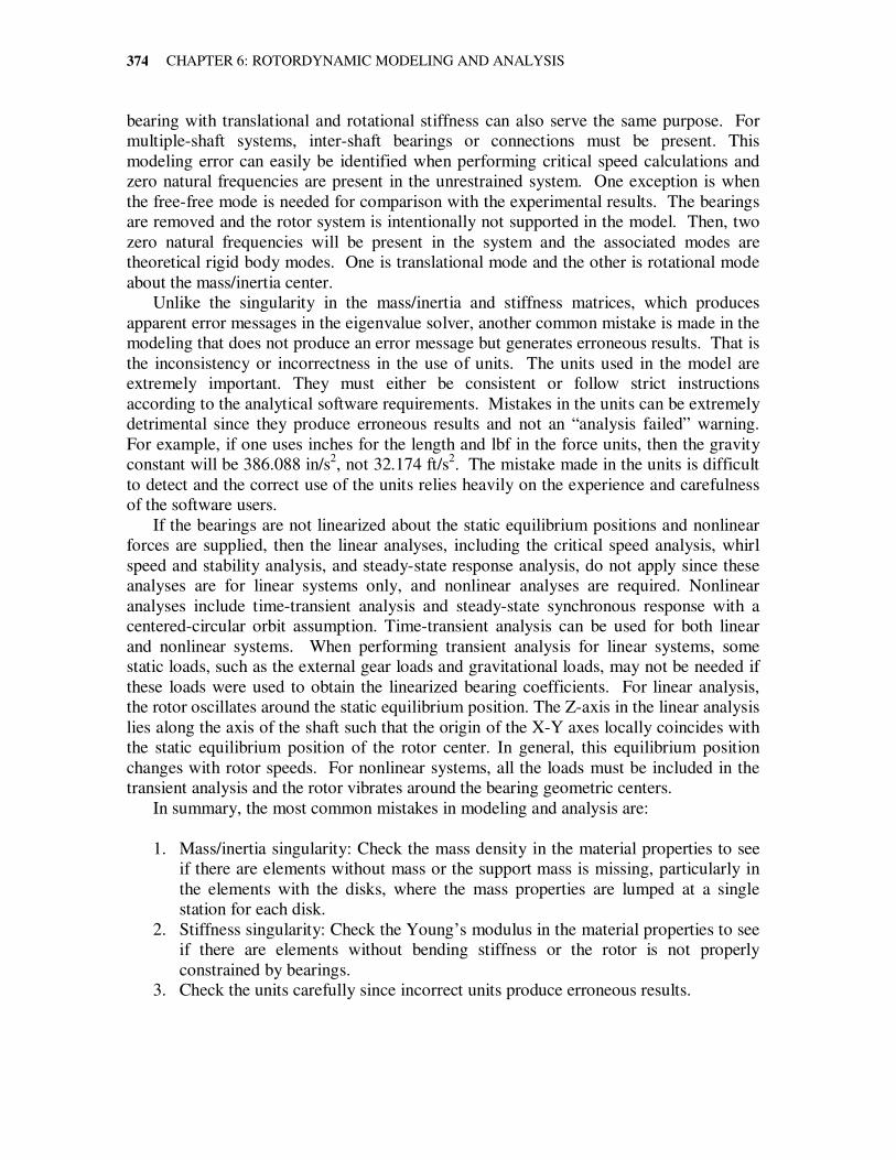
A very similar mistake commonly made in the modeling flexible supports is neglect
of the support mass. As explained earlier, every finite element station requires mass to
produce positive kinetic energy. Therefore, if a flexible support is present, mass is
required at the support station, as illustrated in Figure 6.2-9. Again, there is no need for
as many stations as used here. Although it is not a problem to use so many stations, it is
suggested to use smaller station numbers and employ the sub-elements. By using the
sub-elements, the model will be cleaner and it will be easier to implement local
modifications without affecting the entire system.
Figure 6.2-9 Flexible supports
Another common modeling error involves the singularity of the system stiffness. In
practice, all rotor systems are constrained by bearings or bearing-like mechanisms to
prevent free and unrestrained movement. Without proper constraints, pure rigid body
modes with zero natural frequencies occur and the rotor motion is unbounded. A single-
rotor system is commonly supported by two bearings with translational stiffness to
prevent unrestrained translational and rotational motions. In some applications, one
CHAPTER 6: ROTORDYNAMIC MODELING AND ANALYSIS
374
bearing with translational and rotational stiffness can also serve the same purpose. For
multiple-shaft systems, inter-shaft bearings or connections must be present. This
modeling error can easily be identified when performing critical speed calculations and
zero natural frequencies are present in the unrestrained system. One exception is when
the free-free mode is needed for comparison with the experimental results. The bearings
are removed and the rotor system is intentionally not supported in the model. Then, two
zero natural frequencies will be present in the system and the associated modes are
theoretical rigid body modes. One is translational mode and the other is rotational mode
about the mass/inertia center.
Unlike the singularity in the mass/inertia and stiffness matrices, which produces
apparent error messages in the eigenvalue solver, another common mistake is made in the
modeling that does not produce an error message but generates erroneous results. That is
the inconsistency or incorrectness in the use of units. The units used in the model are
extremely important. They must either be consistent or follow strict instructions
according to the analytical software requirements. Mistakes in the units can be extremely
detrimental since they produce erroneous results and not an “analysis failed” warning.
For example, if one uses inches for the length and lbf in the force units, then the gravity
constant will be 386.088 in/s2, not 32.174 ft/s
2. The mistake made in the units is difficult
to detect and the correct use of the units relies heavily on the experience and carefulness
of the software users.
If the bearings are not linearized about the static equilibrium positions and nonlinear
forces are supplied, then the linear analyses, including the critical speed analysis, whirl
speed and stability analysis, and steady-state response analysis, do not apply since these
analyses are for linear systems only, and nonlinear analyses are required. Nonlinear
analyses include time-transient analysis and steady-state synchronous response with a
centered-circular orbit assumption. Time-transient analysis can be used for both linear
and nonlinear systems. When performing transient analysis for linear systems, some
static loads, such as the external gear loads and gravitational loads, may not be needed if
these loads were used to obtain the linearized bearing coefficients. For linear analysis,
the rotor oscillates around the static equilibrium position. The Z-axis in the linear analysis
lies along the axis of the shaft such that the origin of the X-Y axes locally coincides with
the static equilibrium position of the rotor center. In general, this equilibrium position
changes with rotor speeds. For nonlinear systems, all the loads must be included in the
transient analysis and the rotor vibrates around the bearing geometric centers.
In summary, the most common mistakes in modeling and analysis are:
1. Mass/inertia singularity: Check the mass density in the material properties to see
if there are elements without mass or the support mass is missing, particularly in
the elements with the disks, where the mass properties are lumped at a single
station for each disk.
2. Stiffness singularity: Check the Young’s modulus in the material properties to see
if there are elements without bending stiffness or the rotor is not properly
constrained by bearings.
3. Check the units carefully since incorrect units produce erroneous results.
6.3 STATIC DEFLECTION AND BEARING LOADS
375
4. The critical speed, whirl speed and stability, and steady-state harmonic response
analyses are for linear systems only. If nonlinear components exist in the system,
then nonlinear analyses must be used to study the system dynamic behavior.
5. Linear analyses are based on the assumptions that vibrations are small in the
vicinity of the static equilibrium positions and the system is stable in linear
theory. For systems with large vibrations and negative logarithmic decrements,
nonlinear theory must be applied.
6.3 Static Deflection and Bearing Loads
Static analysis is commonly used to determine the shaft static deflection, bearing
reaction/constrained forces, internal element shear forces and bending moments, and
associated stresses under static external loads, gravitational loads, and geometric
misalignment. It can also be used to verify the accuracy of the model before performing
dynamic analysis. For static deflection and bearing loads, the system generalized force is
a constant and the associated response (deflections) can be obtained from the following
static equation:
o o =K q Q (6.3-1)
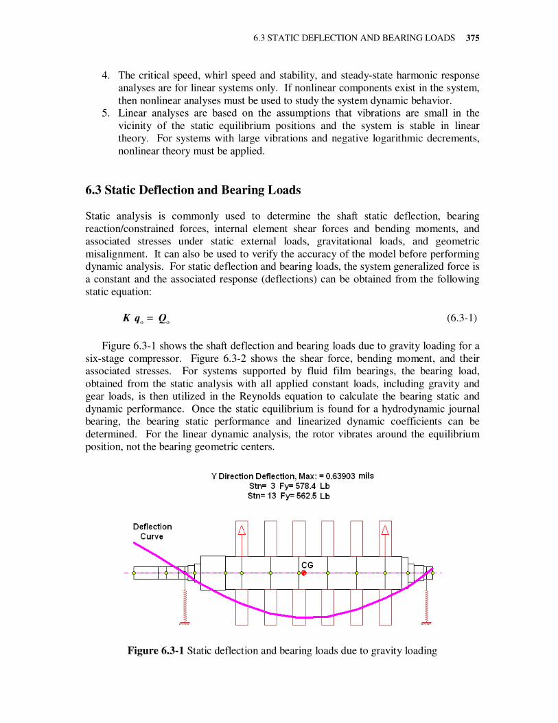
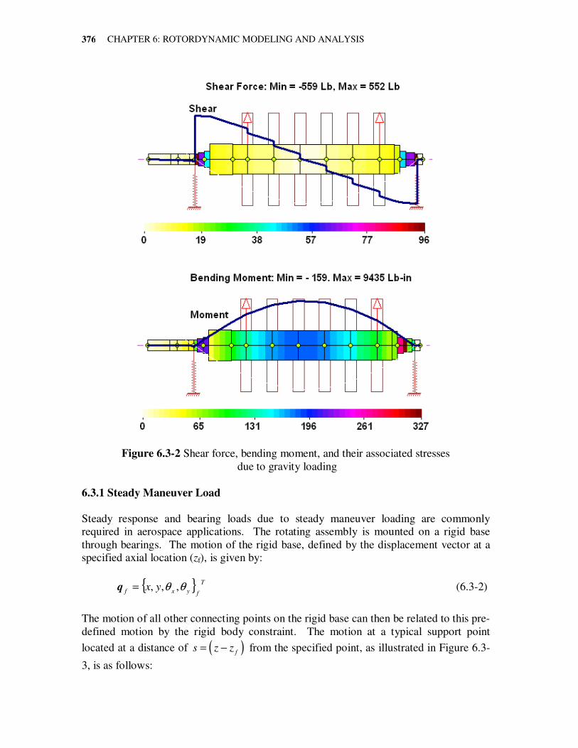
Figure 6.3-1 shows the shaft deflection and bearing loads due to gravity loading for a
six-stage compressor. Figure 6.3-2 shows the shear force, bending moment, and their
associated stresses. For systems supported by fluid film bearings, the bearing load,
obtained from the static analysis with all applied constant loads, including gravity and
gear loads, is then utilized in the Reynolds equation to calculate the bearing static and
dynamic performance. Once the static equilibrium is found for a hydrodynamic journal
bearing, the bearing static performance and linearized dynamic coefficients can be
determined. For the linear dynamic analysis, the rotor vibrates around the equilibrium
position, not the bearing geometric centers.
Figure 6.3-1 Static deflection and bearing loads due to gravity loading
CHAPTER 6: ROTORDYNAMIC MODELING AND ANALYSIS
376
Figure 6.3-2 Shear force, bending moment, and their associated stresses
due to gravity loading
6.3.1 Steady Maneuver Load
Steady response and bearing loads due to steady maneuver loading are commonly
required in aerospace applications. The rotating assembly is mounted on a rigid base
through bearings. The motion of the rigid base, defined by the displacement vector at a
specified axial location (zf), is given by:
T
fyxf yx θθ ,,,=q (6.3-2)
The motion of all other connecting points on the rigid base can then be related to this pre-
defined motion by the rigid body constraint. The motion at a typical support point
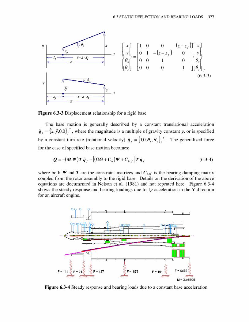
located at a distance of ( )fs z z= − from the specified point, as illustrated in Figure 6.3-
3, is as follows:
6.3 STATIC DEFLECTION AND BEARING LOADS
377
( )( )
fy
x
f
f
y
x
y
x
zz
zz
y
x
−−
−
=
θ
θ
θ
θ
1000
0100
010
001
(6.3-3)
Figure 6.3-3 Displacement relationship for a rigid base
The base motion is generally described by a constant translational acceleration
T
ff yx 0,0,, ɺɺɺɺɺɺ =q , where the magnitude is a multiple of gravity constant g, or is specified
by a constant turn rate (rotational velocity) T
fyxf θθ ɺɺɺ ,,0,0=q . The generalized force
for the case of specified base motion becomes:
( ) ( )[ ] frfbbf qΤCΨCGqTΨMQ ɺɺɺ ,++Ω−−= (6.3-4)
where both ΨΨΨΨ and T are the constraint matrices and Cb,rf is the bearing damping matrix
coupled from the rotor assembly to the rigid base. Details on the derivation of the above
equations are documented in Nelson et al. (1981) and not repeated here. Figure 6.3-4
shows the steady response and bearing loadings due to 1g acceleration in the Y direction
for an aircraft engine.
Figure 6.3-4 Steady response and bearing loads due to a constant base acceleration
CHAPTER 6: ROTORDYNAMIC MODELING AND ANALYSIS
378
6.3.2 Catenary Curve
Static analysis can also be employed to achieve the desirable rotor catenary curve by
adjusting the bearing elevations (misalignments) for a multi-rotor system. The goal is to
keep the bending moments/stresses at the coupling rigid flange faces to a minimum. This
practice is frequently implemented in large turbine-generator units. For a large turbine-
generator system, the coupling station or nearby the coupling location can experience
large moment (stress) during startup. Therefore, at the construction of a turbine-generator
system, the level of each bearing center is adjusted (elevated) to minimize the bending
moment and shear force at each coupling or location where the potential failure may
occur.
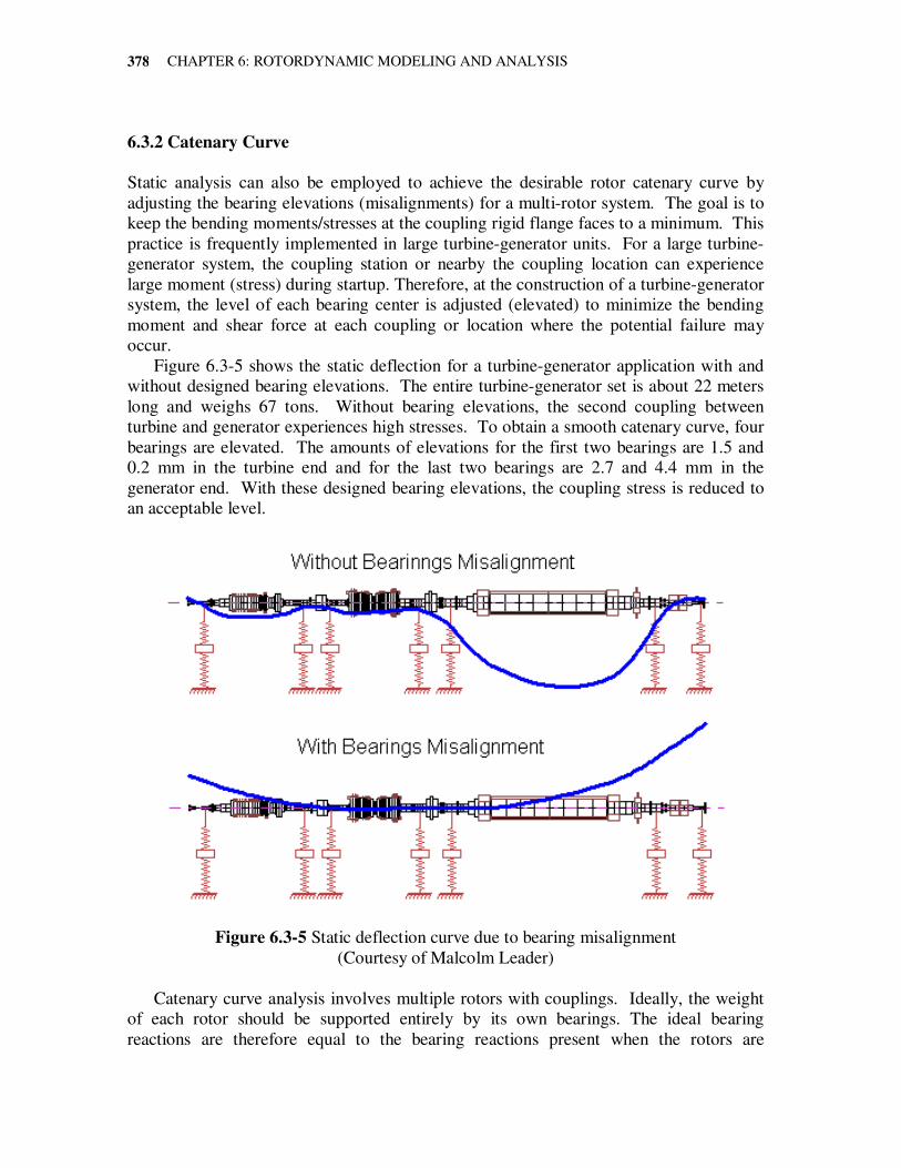
Figure 6.3-5 shows the static deflection for a turbine-generator application with and
without designed bearing elevations. The entire turbine-generator set is about 22 meters
long and weighs 67 tons. Without bearing elevations, the second coupling between
turbine and generator experiences high stresses. To obtain a smooth catenary curve, four
bearings are elevated. The amounts of elevations for the first two bearings are 1.5 and
0.2 mm in the turbine end and for the last two bearings are 2.7 and 4.4 mm in the
generator end. With these designed bearing elevations, the coupling stress is reduced to
an acceptable level.
Figure 6.3-5 Static deflection curve due to bearing misalignment
(Courtesy of Malcolm Leader)
Catenary curve analysis involves multiple rotors with couplings. Ideally, the weight
of each rotor should be supported entirely by its own bearings. The ideal bearing
reactions are therefore equal to the bearing reactions present when the rotors are
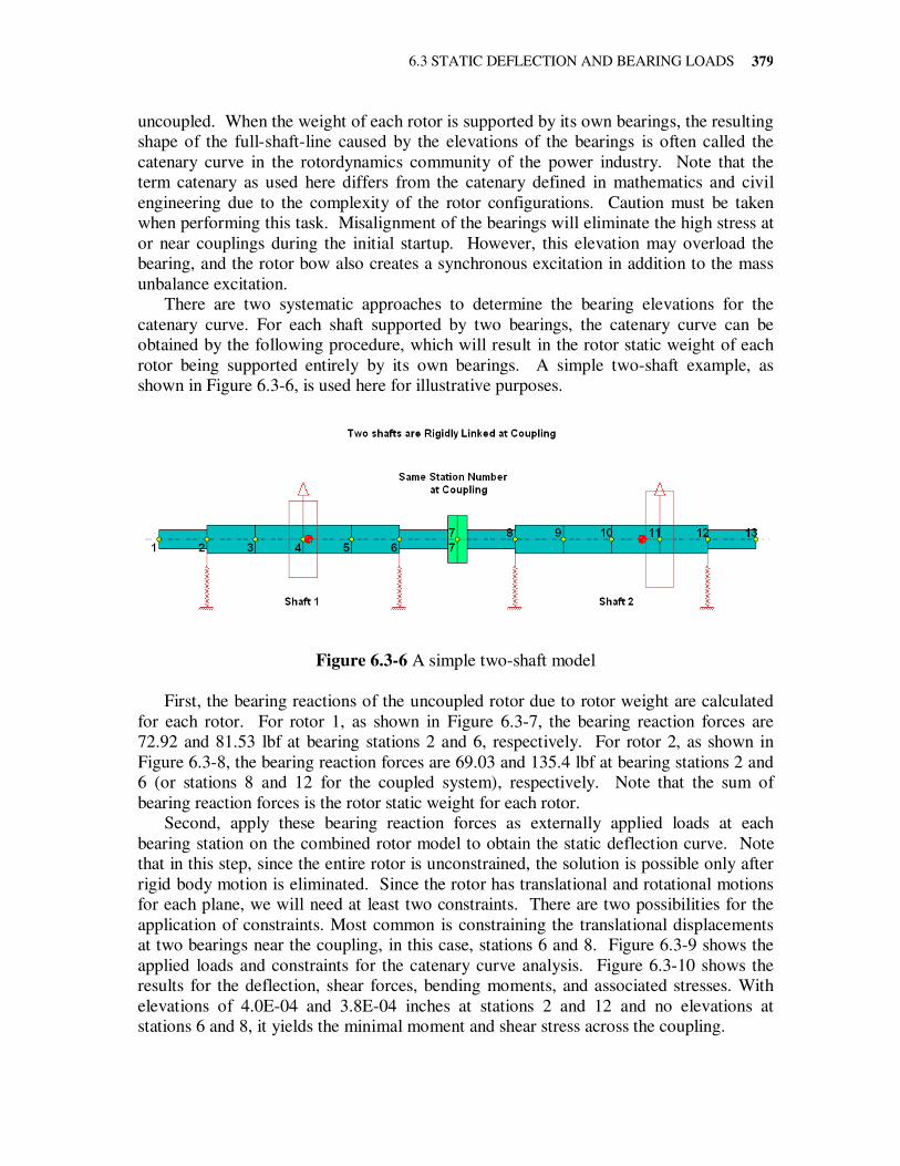
6.3 STATIC DEFLECTION AND BEARING LOADS
379
uncoupled. When the weight of each rotor is supported by its own bearings, the resulting
shape of the full-shaft-line caused by the elevations of the bearings is often called the
catenary curve in the rotordynamics community of the power industry. Note that the
term catenary as used here differs from the catenary defined in mathematics and civil
engineering due to the complexity of the rotor configurations. Caution must be taken
when performing this task. Misalignment of the bearings will eliminate the high stress at
or near couplings during the initial startup. However, this elevation may overload the
bearing, and the rotor bow also creates a synchronous excitation in addition to the mass
unbalance excitation.
There are two systematic approaches to determine the bearing elevations for the
catenary curve. For each shaft supported by two bearings, the catenary curve can be
obtained by the following procedure, which will result in the rotor static weight of each
rotor being supported entirely by its own bearings. A simple two-shaft example, as
shown in Figure 6.3-6, is used here for illustrative purposes.
Figure 6.3-6 A simple two-shaft model
First, the bearing reactions of the uncoupled rotor due to rotor weight are calculated
for each rotor. For rotor 1, as shown in Figure 6.3-7, the bearing reaction forces are
72.92 and 81.53 lbf at bearing stations 2 and 6, respectively. For rotor 2, as shown in
Figure 6.3-8, the bearing reaction forces are 69.03 and 135.4 lbf at bearing stations 2 and
6 (or stations 8 and 12 for the coupled system), respectively. Note that the sum of
bearing reaction forces is the rotor static weight for each rotor.
Second, apply these bearing reaction forces as externally applied loads at each
bearing station on the combined rotor model to obtain the static deflection curve. Note
that in this step, since the entire rotor is unconstrained, the solution is possible only after
rigid body motion is eliminated. Since the rotor has translational and rotational motions
for each plane, we will need at least two constraints. There are two possibilities for the
application of constraints. Most common is constraining the translational displacements
at two bearings near the coupling, in this case, stations 6 and 8. Figure 6.3-9 shows the
applied loads and constraints for the catenary curve analysis. Figure 6.3-10 shows the
results for the deflection, shear forces, bending moments, and associated stresses. With
elevations of 4.0E-04 and 3.8E-04 inches at stations 2 and 12 and no elevations at
stations 6 and 8, it yields the minimal moment and shear stress across the coupling.
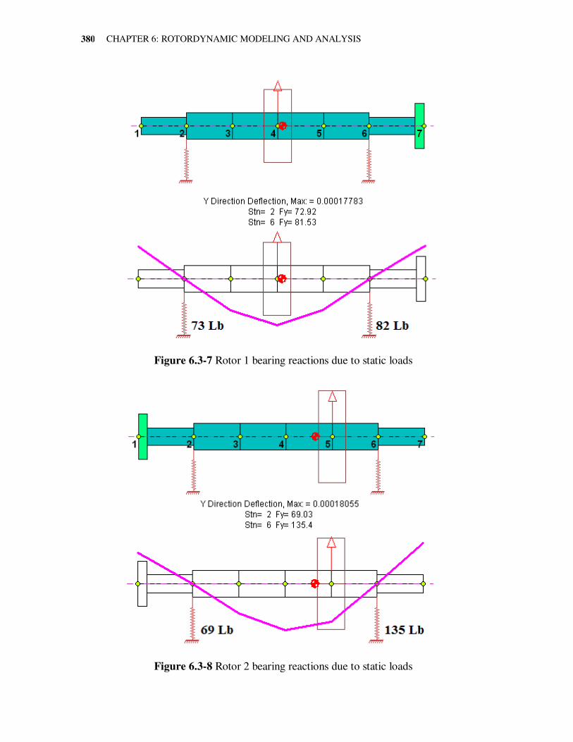
CHAPTER 6: ROTORDYNAMIC MODELING AND ANALYSIS
380
Figure 6.3-7 Rotor 1 bearing reactions due to static loads
Figure 6.3-8 Rotor 2 bearing reactions due to static loads
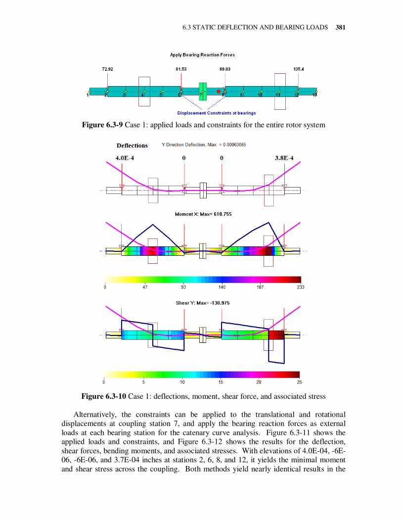
6.3 STATIC DEFLECTION AND BEARING LOADS
381
Figure 6.3-9 Case 1: applied loads and constraints for the entire rotor system
Figure 6.3-10 Case 1: deflections, moment, shear force, and associated stress
Alternatively, the constraints can be applied to the translational and rotational
displacements at coupling station 7, and apply the bearing reaction forces as external
loads at each bearing station for the catenary curve analysis. Figure 6.3-11 shows the
applied loads and constraints, and Figure 6.3-12 shows the results for the deflection,
shear forces, bending moments, and associated stresses. With elevations of 4.0E-04, -6E-
06, -6E-06, and 3.7E-04 inches at stations 2, 6, 8, and 12, it yields the minimal moment
and shear stress across the coupling. Both methods yield nearly identical results in the
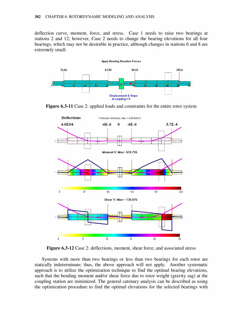
CHAPTER 6: ROTORDYNAMIC MODELING AND ANALYSIS
382
deflection curve, moment, force, and stress. Case 1 needs to raise two bearings at
stations 2 and 12; however, Case 2 needs to change the bearing elevations for all four
bearings, which may not be desirable in practice, although changes in stations 6 and 8 are
extremely small.
Figure 6.3-11 Case 2: applied loads and constraints for the entire rotor system
Figure 6.3-12 Case 2: deflections, moment, shear force, and associated stress
Systems with more than two bearings or less than two bearings for each rotor are
statically indeterminate; thus, the above approach will not apply. Another systematic
approach is to utilize the optimization technique to find the optimal bearing elevations,
such that the bending moment and/or shear force due to rotor weight (gravity sag) at the
coupling station are minimized. The general catenary analysis can be described as using
the optimization procedure to find the optimal elevations for the selected bearings with
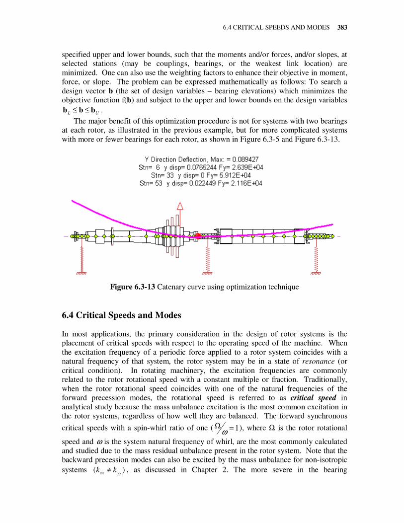
6.4 CRITICAL SPEEDS AND MODES
383
specified upper and lower bounds, such that the moments and/or forces, and/or slopes, at
selected stations (may be couplings, bearings, or the weakest link location) are
minimized. One can also use the weighting factors to enhance their objective in moment,
force, or slope. The problem can be expressed mathematically as follows: To search a
design vector b (the set of design variables – bearing elevations) which minimizes the
objective function f(b) and subject to the upper and lower bounds on the design variables
L U≤ ≤b b b .
The major benefit of this optimization procedure is not for systems with two bearings
at each rotor, as illustrated in the previous example, but for more complicated systems
with more or fewer bearings for each rotor, as shown in Figure 6.3-5 and Figure 6.3-13.
Figure 6.3-13 Catenary curve using optimization technique
6.4 Critical Speeds and Modes
In most applications, the primary consideration in the design of rotor systems is the
placement of critical speeds with respect to the operating speed of the machine. When
the excitation frequency of a periodic force applied to a rotor system coincides with a
natural frequency of that system, the rotor system may be in a state of resonance (or
critical condition). In rotating machinery, the excitation frequencies are commonly
related to the rotor rotational speed with a constant multiple or fraction. Traditionally,
when the rotor rotational speed coincides with one of the natural frequencies of the
forward precession modes, the rotational speed is referred to as critical speed in
analytical study because the mass unbalance excitation is the most common excitation in
the rotor systems, regardless of how well they are balanced. The forward synchronous
critical speeds with a spin-whirl ratio of one ( 1=Ωω ), where Ω is the rotor rotational
speed and ω is the system natural frequency of whirl, are the most commonly calculated
and studied due to the mass residual unbalance present in the rotor system. Note that the
backward precession modes can also be excited by the mass unbalance for non-isotropic
systems ( )xx yy
k k≠ , as discussed in Chapter 2. The more severe in the bearing
CHAPTER 6: ROTORDYNAMIC MODELING AND ANALYSIS
384
asymmetric properties, the easier the backward precession modes will be excited (Chen
& Gunter, 2005). To calculate the backward synchronous critical speeds, a spin-whirl
ratio of minus one ( 1ωΩ = − ) is used. Other common synchronous excitations include
excitations due to shaft bow, disk skew, and coupling misalignment. Non-synchronous
excitations include aerodynamic excitations for compressors, gear mesh excitations for
geared systems, vane passing excitation, and electrical wiring excitation, among others.
In industrial practice, the critical speeds are the rotor speeds where the measured peak
responses are observed. Based on this definition, the critical speeds will depend on the
system damping, axial and angular position of the measurements (vibration probes), and
other operating conditions. When the critical speeds are within the operating speed
range, the rotor may experience large synchronous vibration if system damping is small.
For highly damped systems, the calculated critical speeds may not even be observed in
the real machine, and there are no apparent peaks in the response curve. It is desirable to
have separation margins between the operating speed range and the calculated critical
speeds for safe and smooth operation. The bearing stiffness is likely the most common
design parameter to ensure a safe separation margin between the critical speeds and the
rotor design operating speed.
The assumptions for the typical critical speed analysis are that the system is isotropic
and undamped (conservative) and that bearing stiffness is constant (speed-independent
bearing properties). A detailed definition of undamped isotropic bearings was described
in Chapter 2. However, it is known that the linearized fluid film bearing forces contain
the non-isotropic and speed-dependent damping and stiffness coefficients. Due to the
simplified assumptions applied in the critical speed calculation, extreme care must be
taken in preparing and interpreting these results. Caution must also be taken when
utilizing this simplified technique to estimate the critical speeds where the peak responses
occur, especially for highly damped and non-isotropic systems. Very often, the peak
response does not occur at the calculated critical speeds due to these simplified
assumptions. This analysis only provides a reference for design purposes.
For undamped rotor systems with isotropic and speed-independent support properties,
the analytical critical speeds may be determined directly from a reduced eigenvalue
problem associated with the system equations expressed in a rotating reference frame.
These undamped modes are circular relative to the fixed reference frame but constant
relative to the rotating reference frame. Therefore, it is convenient to analyze only one of
the two planes of motion (X-Z or Y-Z). The undamped natural circular whirl speeds and
mode shapes can be obtained from the homogeneous form of system equations expressed
in the rotating reference frame. Assuming a constant eigensolution, the reduced
eigenvalue problem in the (X-Z) plane can be written as follows:
( ) 0 2 =− iXZiXZ yMK ω (6.4-1)
where 2 ( 1, 2,.... )i
i Nω = are called eigenvalues, and iω are recognized as the natural whirl
frequencies of the system, or critical speeds in this case. The vectors iy are the
associated (right) eigenvectors or mode shapes. N is the dimension (order) of the reduced
system matrices (N=NDOF/2). For a conservative system, the matrices Kxz and Mxz are
all symmetric, and the generalized mass/inertia matrix Mxz is a function of the spin-whirl
6.4 CRITICAL SPEEDS AND MODES
385
ratio ω
γΩ
= . The subscript (XZ) denotes that only one plane of motion is considered,
which can be either the (XZ) or the (YZ) plane of motion. The spin-whirl ratio in the
reduced mass matrix is derived from the gyroscopic effect. The spin/whirl ratio must be
specified in advance to determine various types of critical speeds. The typical values and
types of critical speeds are:
1=γ Forward synchronous critical speeds
1−=γ Backward synchronous critical speeds
0=γ Planar critical speeds for non-rotating systems (Ω=0)
2=γ Half-frequency whirl (sub-synchronous critical speeds, 1
2ωΩ = )
1n
γ = Forward super-synchronous critical speeds ( n ωΩ = )
Unless specified otherwise, forward synchronous critical speeds ( 1=γ ) are used in
this text and also in industrial practice. Since the critical speed analysis is based on
undamped and isotropic systems, the bearing dynamic stiffness (the combination of
bearing stiffness and damping) should be used in the critical speed calculation and is
defined as:
( )22 CKK d ω+= (6.4-2)
For rotor systems with speed-dependent bearing coefficients, an iterative process is
required to determine the critical speeds. The critical speeds can also be determined
graphically by examining the critical speed map with the bearing dynamic stiffness
superimposed on the map.
Let us assume that the six-stage compressor presented previously is supported by two
identical ball bearings with a stiffness value of 5.0E05 Lbf/in. The first three undamped
forward synchronous critical speeds are calculated, and their associated mode shapes and
potential energy distribution are shown in Figure 6.4-1. In this example, the first critical
mode with a whirling frequency of 4,654 rpm is not a classical rigid rotor mode or a
purely flexible rotor mode. It does not have nodal points across the shaft centerline and
there is about 30% of the potential energy in the flexible shaft. It has characteristics of
both rigid and flexible rotor modes, although its behavior is closer to a rigid rotor because
of 70% of the potential energy occurring in the bearings. The second mode with a
whirling frequency of 10,420 rpm can be classified as a rigid rotor mode with only about
10% of the potential energy in the shaft, which is less than in the first mode. Although
this mode has a nodal point across the shaft centerline, it is essentially a rigid rotor mode
(rotatory or conical mode), which is rocking about the center of mass (nodal point in this
case). Note that the second mode has a smaller potential energy percentage and less
bending in the shaft, but a higher whirling frequency than the first mode in this example.
Therefore, it is not always the mode with the smaller potential energy in the shaft that has
the lower natural frequency. The third mode has two nodal points and is a flexible rotor
(bending) mode with 87% of the potential energy in the flexible shaft.
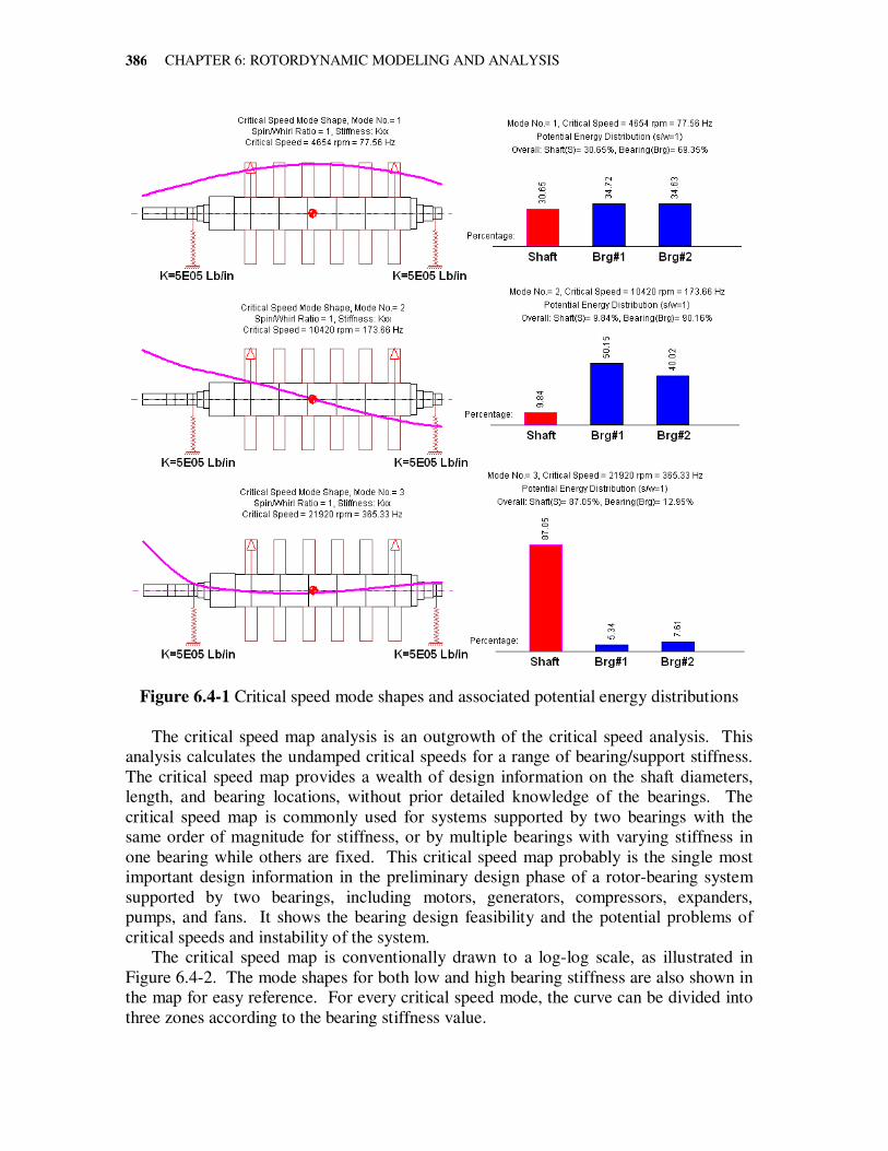
CHAPTER 6: ROTORDYNAMIC MODELING AND ANALYSIS
386
Figure 6.4-1 Critical speed mode shapes and associated potential energy distributions
The critical speed map analysis is an outgrowth of the critical speed analysis. This
analysis calculates the undamped critical speeds for a range of bearing/support stiffness.
The critical speed map provides a wealth of design information on the shaft diameters,
length, and bearing locations, without prior detailed knowledge of the bearings. The
critical speed map is commonly used for systems supported by two bearings with the
same order of magnitude for stiffness, or by multiple bearings with varying stiffness in
one bearing while others are fixed. This critical speed map probably is the single most
important design information in the preliminary design phase of a rotor-bearing system
supported by two bearings, including motors, generators, compressors, expanders,
pumps, and fans. It shows the bearing design feasibility and the potential problems of
critical speeds and instability of the system.
The critical speed map is conventionally drawn to a log-log scale, as illustrated in
Figure 6.4-2. The mode shapes for both low and high bearing stiffness are also shown in
the map for easy reference. For every critical speed mode, the curve can be divided into
three zones according to the bearing stiffness value.
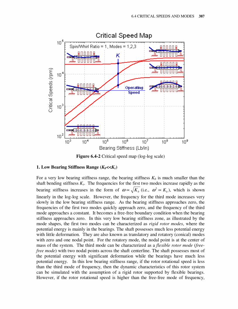
6.4 CRITICAL SPEEDS AND MODES
387
Figure 6.4-2 Critical speed map (log-log scale)
1. Low Bearing Stiffness Range (Kb<<Ks)
For a very low bearing stiffness range, the bearing stiffness Kb is much smaller than the
shaft bending stiffness Ks. The frequencies for the first two modes increase rapidly as the
bearing stiffness increases in the form of bK∝ω (i.e., 2
bKω ∝ ), which is shown
linearly in the log-log scale. However, the frequency for the third mode increases very
slowly in the low bearing stiffness range. As the bearing stiffness approaches zero, the
frequencies of the first two modes quickly approach zero, and the frequency of the third
mode approaches a constant. It becomes a free-free boundary condition when the bearing
stiffness approaches zero. In this very low bearing stiffness zone, as illustrated by the
mode shapes, the first two modes can be characterized as rigid rotor modes, where the
potential energy is mainly in the bearings. The shaft possesses much less potential energy
with little deformation. They are also known as translatory and rotatory (conical) modes
with zero and one nodal point. For the rotatory mode, the nodal point is at the center of
mass of the system. The third mode can be characterized as a flexible rotor mode (free-
free mode) with two nodal points across the shaft centerline. The shaft possesses most of
the potential energy with significant deformation while the bearings have much less
potential energy. In this low bearing stiffness range, if the rotor rotational speed is less
than the third mode of frequency, then the dynamic characteristics of this rotor system
can be simulated with the assumption of a rigid rotor supported by flexible bearings.
However, if the rotor rotational speed is higher than the free-free mode of frequency,
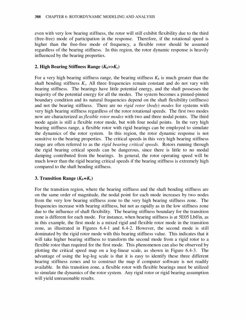
CHAPTER 6: ROTORDYNAMIC MODELING AND ANALYSIS
388
even with very low bearing stiffness, the rotor will still exhibit flexibility due to the third
(free-free) mode of participation in the response. Therefore, if the rotational speed is
higher than the free-free mode of frequency, a flexible rotor should be assumed
regardless of the bearing stiffness. In this region, the rotor dynamic response is heavily
influenced by the bearing properties.
2. High Bearing Stiffness Range (Kb>>Ks)
For a very high bearing stiffness range, the bearing stiffness Kb is much greater than the
shaft bending stiffness Ks. All three frequencies remain constant and do not vary with
bearing stiffness. The bearings have little potential energy, and the shaft possesses the
majority of the potential energy for all the modes. The system becomes a pinned-pinned
boundary condition and its natural frequencies depend on the shaft flexibility (stiffness)
and not the bearing stiffness. There are no rigid rotor (body) modes for systems with
very high bearing stiffness regardless of the rotor rotational speeds. The first two modes
now are characterized as flexible rotor modes with two and three nodal points. The third
mode again is still a flexible rotor mode, but with four nodal points. In the very high
bearing stiffness range, a flexible rotor with rigid bearings can be employed to simulate
the dynamics of the rotor system. In this region, the rotor dynamic response is not
sensitive to the bearing properties. The critical speeds in this very high bearing stiffness
range are often referred to as the rigid bearing critical speeds. Rotors running through
the rigid bearing critical speeds can be dangerous, since there is little to no modal
damping contributed from the bearings. In general, the rotor operating speed will be
much lower than the rigid bearing critical speeds if the bearing stiffness is extremely high
compared to the shaft bending stiffness.
3. Transition Range (Kb≈≈≈≈ Ks)
For the transition region, where the bearing stiffness and the shaft bending stiffness are
on the same order of magnitude, the nodal point for each mode increases by two nodes
from the very low bearing stiffness zone to the very high bearing stiffness zone. The
frequencies increase with bearing stiffness, but not as rapidly as in the low stiffness zone
due to the influence of shaft flexibility. The bearing stiffness boundary for the transition
zone is different for each mode. For instance, when bearing stiffness is at 5E05 Lbf/in, as
in this example, the first mode is a mixed rigid and flexible rotor mode in the transition
zone, as illustrated in Figures 6.4-1 and 6.4-2. However, the second mode is still
dominated by the rigid rotor mode with this bearing stiffness value. This indicates that it
will take higher bearing stiffness to transform the second mode from a rigid rotor to a
flexible rotor than required for the first mode. This phenomenon can also be observed by
plotting the critical speed map on a log-linear scale, as shown in Figure 6.4-3. The
advantage of using the log-log scale is that it is easy to identify these three different
bearing stiffness zones and to construct the map if computer software is not readily
available. In this transition zone, a flexible rotor with flexible bearings must be utilized
to simulate the dynamics of the rotor system. Any rigid rotor or rigid bearing assumption
will yield unreasonable results.
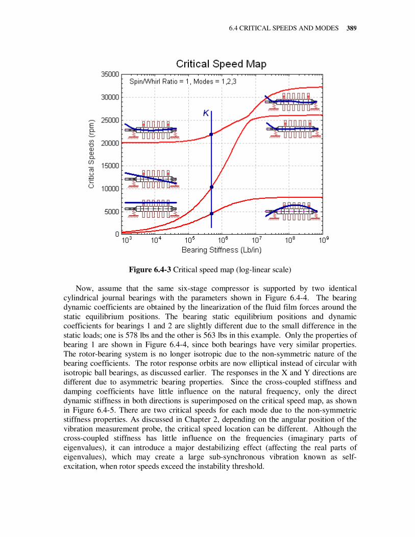
6.4 CRITICAL SPEEDS AND MODES
389
Figure 6.4-3 Critical speed map (log-linear scale)
Now, assume that the same six-stage compressor is supported by two identical
cylindrical journal bearings with the parameters shown in Figure 6.4-4. The bearing
dynamic coefficients are obtained by the linearization of the fluid film forces around the
static equilibrium positions. The bearing static equilibrium positions and dynamic
coefficients for bearings 1 and 2 are slightly different due to the small difference in the
static loads; one is 578 lbs and the other is 563 lbs in this example. Only the properties of
bearing 1 are shown in Figure 6.4-4, since both bearings have very similar properties.
The rotor-bearing system is no longer isotropic due to the non-symmetric nature of the
bearing coefficients. The rotor response orbits are now elliptical instead of circular with
isotropic ball bearings, as discussed earlier. The responses in the X and Y directions are
different due to asymmetric bearing properties. Since the cross-coupled stiffness and
damping coefficients have little influence on the natural frequency, only the direct
dynamic stiffness in both directions is superimposed on the critical speed map, as shown
in Figure 6.4-5. There are two critical speeds for each mode due to the non-symmetric
stiffness properties. As discussed in Chapter 2, depending on the angular position of the
vibration measurement probe, the critical speed location can be different. Although the
cross-coupled stiffness has little influence on the frequencies (imaginary parts of
eigenvalues), it can introduce a major destabilizing effect (affecting the real parts of
eigenvalues), which may create a large sub-synchronous vibration known as self-
excitation, when rotor speeds exceed the instability threshold.
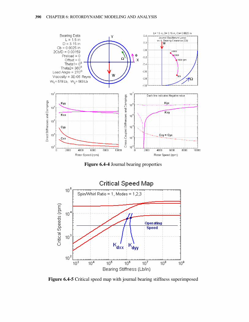
CHAPTER 6: ROTORDYNAMIC MODELING AND ANALYSIS
390
Figure 6.4-4 Journal bearing properties
Figure 6.4-5 Critical speed map with journal bearing stiffness superimposed
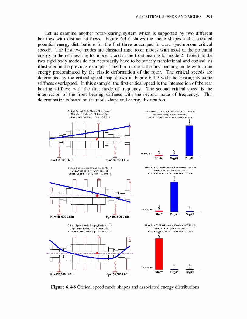
6.4 CRITICAL SPEEDS AND MODES
391
Let us examine another rotor-bearing system which is supported by two different
bearings with distinct stiffness. Figure 6.4-6 shows the mode shapes and associated
potential energy distributions for the first three undamped forward synchronous critical
speeds. The first two modes are classical rigid rotor modes with most of the potential
energy in the rear bearing for mode 1, and in the front bearing for mode 2. Note that the
two rigid body modes do not necessarily have to be strictly translational and conical, as
illustrated in the previous example. The third mode is the first bending mode with strain
energy predominated by the elastic deformation of the rotor. The critical speeds are
determined by the critical speed map shown in Figure 6.4-7 with the bearing dynamic
stiffness overlapped. In this example, the first critical speed is the intersection of the rear
bearing stiffness with the first mode of frequency. The second critical speed is the
intersection of the front bearing stiffness with the second mode of frequency. This
determination is based on the mode shape and energy distribution.
Figure 6.4-6 Critical speed mode shapes and associated energy distributions
CHAPTER 6: ROTORDYNAMIC MODELING AND ANALYSIS
392
Figure 6.4-7 Critical speed map
6.5 Steady-State Harmonic Response
The steady-state synchronous excitations are the most common excitations in rotating
machinery. Therefore, the majority of the discussion in this section is focused on the
synchronous response. However, asynchronous harmonic excitations are also present in
some applications and attention to them is also needed. Figure 6.5-1 shows vibration data
taken during machine shutdown for a centrifugal compressor. This plot of vibration
amplitude versus machine rotating speed and frequency is commonly referred to as a
waterfall plot or cascade plot. Every trace of a curve is a Fast Fourier Transform (FFT) at
a rotational speed. The dominant vibration is the synchronous vibration and vibrations at
other frequency components are very small. The operating speed is 12,800 rpm and the
critical speed is around 7,500 rpm, which can be observed from the synchronous
vibration curve. This observed critical speed is caused by the mass unbalance.
Figure 6.5-2 shows a waterfall plot for a rotary screw compressor during startup. The
dominant components are 2×, 4×, and 8× non-synchronous harmonics, and synchronous
vibration is insignificant in this case. The rotor operating speed is between 1,200 and
3,300 rpm. The forward synchronous critical speed due to mass unbalance is around
5,600 rpm, which is far above the rotor operating speed, and not shown in the
measurement data. However, there are strong super-synchronous excitations, 4× and 8×
components, due to the overhung motor excitations that cause high vibrations when rotor
speeds are near 700 and 1,400 rpm. These two speeds are also called critical speeds;
however, they are not caused by mass unbalance, but by excitations from the motor
electrical source.
6.5 STEADY-STATE HARMONIC RESPONSE
393
Figure 6.5-1 Waterfall plot to show the dominant synchronous vibrations
Figure 6.5-2 Waterfall plot to show the dominant non-synchronous vibrations
The solution techniques are the same for both the synchronous and non-synchronous
harmonic steady-state response. For linear analysis, the shaft oscillates around its static
equilibrium position, which is different from the true bearing geometric center line. For
small vibrations, the shaft position can be approximated by the superposition of the static
equilibrium position and the steady-state response.
CHAPTER 6: ROTORDYNAMIC MODELING AND ANALYSIS
394
6.5.1 Steady-State Synchronous Response
The common steady-state synchronous excitations in rotating machinery include mass
unbalance, disk skew, shaft bow, and coupling misalignment. For synchronous
excitations, the excitation frequency is the same as the shaft rotational speed, ωexc = Ω.
The steady-state synchronous excitation can be written in the following form:
( )αQQQQ +Ω=Ω+Ω= ttt sc cossincos (6.5-1)
where Q is the magnitude of the excitation and αααα is the angle specifying the angular
position of the excitations measured in the direction of rotation. For linear systems, the
steady-state synchronous response, commonly referred to as the 1× vibration, has the
same form:
( )cos sin cosc s
t t t φ= Ω + Ω = Ω −q q q q (6.5-2)
where q is the amplitude of the response and φφφφ is the phase angle. Note that the
negative sign is employed in Eq. (6.5-2) for the response phase angle. Since the response
lags the excitation, a negative sign in the phase angle expression is commonly used to
indicate the phase lag. That is, a positive phase angle φφφφ indicates the opposite direction
of rotation, and a negative phase angle (-φφφφ ) indicates the direction of rotation. The
steady-state response lags the excitation by a phase angle of (φφφφ+αααα), which is commonly
referred to as the phase lag angle. Figure 6.5-3 shows the relationship of two rotating
vectors; their projections onto the real axis are the excitation and response expressed in
Eqs. (6.5-1) and (6.5-2). The phase lag angle between the excitation and response (φφφφ+αααα)
has a range from 0o to 180
o. For undamped systems, the phase lag angle is either in-
phase (0o) or out-of-phase (180
o). Phase angle is an important parameter used in
balancing and machine malfunction diagnosis, as discussed in Chapter 2.
Figure 6.5-3 Phase relationship between the excitation and response
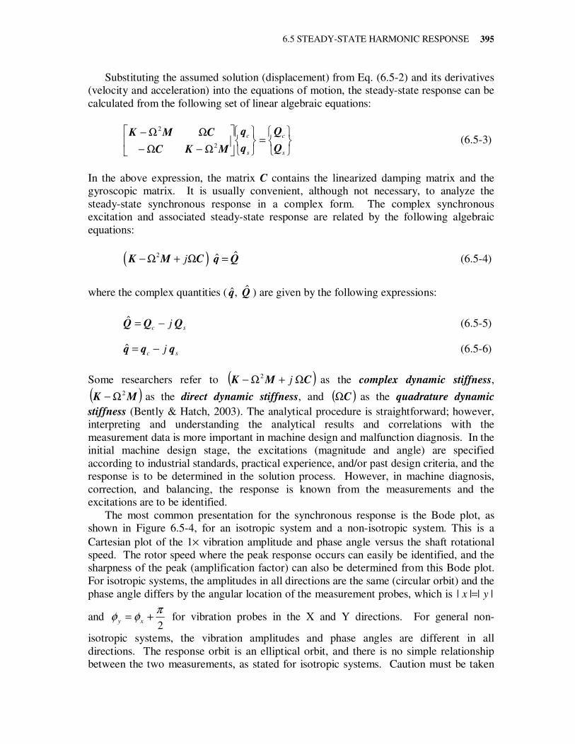
6.5 STEADY-STATE HARMONIC RESPONSE
395
Substituting the assumed solution (displacement) from Eq. (6.5-2) and its derivatives
(velocity and acceleration) into the equations of motion, the steady-state response can be
calculated from the following set of linear algebraic equations:
=
Ω−Ω−
ΩΩ−
s
c
s
c
Q
Q
q
q
MKC
CMK2
2
(6.5-3)
In the above expression, the matrix C contains the linearized damping matrix and the
gyroscopic matrix. It is usually convenient, although not necessary, to analyze the
steady-state synchronous response in a complex form. The complex synchronous
excitation and associated steady-state response are related by the following algebraic
equations:
( )2 ˆˆ j− Ω + Ω =K M C q Q (6.5-4)
where the complex quantities ( Qq ˆ ,ˆ ) are given by the following expressions:
sc j QQQ ˆ −= (6.5-5)
sc j qqq ˆ −= (6.5-6)
Some researchers refer to ( ) 2 CMK Ω+Ω− j as the complex dynamic stiffness,
( ) 2 MK Ω− as the direct dynamic stiffness, and ( ) CΩ as the quadrature dynamic
stiffness (Bently & Hatch, 2003). The analytical procedure is straightforward; however,
interpreting and understanding the analytical results and correlations with the
measurement data is more important in machine design and malfunction diagnosis. In the
initial machine design stage, the excitations (magnitude and angle) are specified
according to industrial standards, practical experience, and/or past design criteria, and the
response is to be determined in the solution process. However, in machine diagnosis,
correction, and balancing, the response is known from the measurements and the
excitations are to be identified.
The most common presentation for the synchronous response is the Bode plot, as
shown in Figure 6.5-4, for an isotropic system and a non-isotropic system. This is a
Cartesian plot of the 1× vibration amplitude and phase angle versus the shaft rotational
speed. The rotor speed where the peak response occurs can easily be identified, and the
sharpness of the peak (amplification factor) can also be determined from this Bode plot.
For isotropic systems, the amplitudes in all directions are the same (circular orbit) and the
phase angle differs by the angular location of the measurement probes, which is |||| yx =
and 2
πφφ +=
xy for vibration probes in the X and Y directions. For general non-
isotropic systems, the vibration amplitudes and phase angles are different in all
directions. The response orbit is an elliptical orbit, and there is no simple relationship
between the two measurements, as stated for isotropic systems. Caution must be taken
CHAPTER 6: ROTORDYNAMIC MODELING AND ANALYSIS
396
when determining the critical speeds by examining the Bode plot for non-isotropic
systems because the peak response occurs at different speeds for probes at different
angular locations.
Figure 6.5-4 Typical Bode plots for isotropic and non-isotropic systems
Another presentation for the steady-state synchronous response is the polar plot,
which is used frequently to present measurement vibration data and less often to present
analytical results. It is the response locus of the 1× vibration (amplitude and phase)
versus speeds at a specific direction (or probe location) in the polar coordinate system.
Note that the phase angle is labeled against the direction of shaft rotation, since the
response always lags the excitation. The polar plot is commonly used for balancing
purposes, and the graph is rotated to align the zero phase angle with the probe physical
location, as shown in Figure 6.5-5. By properly aligning the probe physical location with
the zero phase angle, the response locus is identical for any probe location at a specific
rotor plane in the polar plot for isotropic systems, as shown in Figure 6.5-5. For non-
isotropic systems, the plots will differ for different probe angles, as illustrated in Figure
6.5-5.
6.5 STEADY-STATE HARMONIC RESPONSE
397
Figure 6.5-5 Typical polar plots for isotropic and non-isotropic systems
Consider the six-stage compressor system supported by two identical ball bearings
with K=5.0E05 Lbf/in and C=10 Lbf-s/in, and assume an unbalance of 5 oz-in at stages 1
and 6 with the same angular position. From the mode shapes shown in Figure 6.4-1, the
two unbalance forces with the same angle will excite the first mode; however, the
resulting excitation force for the second mode is nearly canceled out due to the modal
displacements at both excitation locations being out-of-phase. The Bode plots of the
steady-state unbalance response at both bearings are shown in Figure 6.5-6. The response
amplitudes in the X and Y directions are identical, and the phases are 90o different for
this isotropic system. The response orbits are circular. The first peak response occurs at
4,654 rpm and the second critical speed is not observed due to the extremely small net
modal excitation force. These results are consistent with the mode shapes shown in
Figure 6.4-1. The responses near the first critical speed are enlarged in Figure 6.5-7 to
illustrate the definition of the amplification factor using half-power points.
Figure 6.5-6 Steady-state unbalance response with roller bearings
CHAPTER 6: ROTORDYNAMIC MODELING AND ANALYSIS
398
Figure 6.5-7 Steady-state unbalance response for amplification factor
As indicated in the Bode plot, the peak response and amplification factor at critical
speed can be very high for this lightly damped system. Fortunately, the operating speed
of this compressor is at 2,975 rpm for a 50 Hz motor driver and 3,575 rpm for a 60 Hz
motor driver, which is far below the first critical speed with 56% and 30% separation
margins, respectively. The complete rotor steady-state response at 2,975 rpm is shown in
Figure 6.5-8. The rotor response is similar at 3,575 rpm and not shown again.
Figure 6.5-8 Steady-state unbalance response with roller bearings at design speed
The Bode plots for the same rotor system supported by two fluid film bearings with
linearized bearing coefficients, as presented in Figure 6.4-4, are shown in Figure 6.5-9.
The fluid film bearings provide good direct damping, which attenuates the synchronous
vibrations. For this highly damped system with non-symmetric bearing properties, the
peak responses occur at different rotor speeds for different rotor stations. Even at the
same station, the response differs at different angular positions due to the bearing
asymmetric properties. The rotor response orbits at a design speed of 2,975 rpm are
elliptical for this non-isotropic system, as shown in Figure 6.5-10. The amplification
factor cannot be calculated since the N2 point is not available for speeds up to 10,000 rpm
due to the high damping in this case. The system is called critically damped.
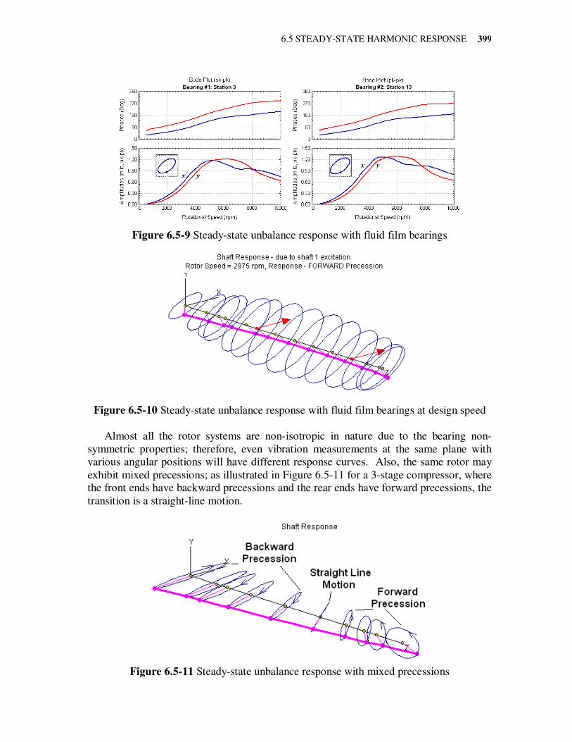
6.5 STEADY-STATE HARMONIC RESPONSE
399
Figure 6.5-9 Steady-state unbalance response with fluid film bearings
Figure 6.5-10 Steady-state unbalance response with fluid film bearings at design speed
Almost all the rotor systems are non-isotropic in nature due to the bearing non-
symmetric properties; therefore, even vibration measurements at the same plane with
various angular positions will have different response curves. Also, the same rotor may
exhibit mixed precessions; as illustrated in Figure 6.5-11 for a 3-stage compressor, where
the front ends have backward precessions and the rear ends have forward precessions, the
transition is a straight-line motion.
Figure 6.5-11 Steady-state unbalance response with mixed precessions
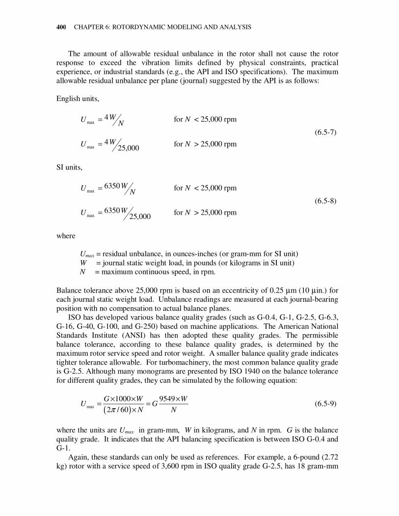
CHAPTER 6: ROTORDYNAMIC MODELING AND ANALYSIS
400
The amount of allowable residual unbalance in the rotor shall not cause the rotor
response to exceed the vibration limits defined by physical constraints, practical
experience, or industrial standards (e.g., the API and ISO specifications). The maximum
allowable residual unbalance per plane (journal) suggested by the API is as follows:
English units,
N
WU 4max = for N < 25,000 rpm
(6.5-7)
000,25
4max
WU = for N > 25,000 rpm
SI units,
N
WU 6350max = for N < 25,000 rpm
(6.5-8)
000,25
6350max
WU = for N > 25,000 rpm
where
Umax = residual unbalance, in ounces-inches (or gram-mm for SI unit)
W = journal static weight load, in pounds (or kilograms in SI unit)
N = maximum continuous speed, in rpm.
Balance tolerance above 25,000 rpm is based on an eccentricity of 0.25 µm (10 µin.) for
each journal static weight load. Unbalance readings are measured at each journal-bearing
position with no compensation to actual balance planes.
ISO has developed various balance quality grades (such as G-0.4, G-1, G-2.5, G-6.3,
G-16, G-40, G-100, and G-250) based on machine applications. The American National
Standards Institute (ANSI) has then adopted these quality grades. The permissible
balance tolerance, according to these balance quality grades, is determined by the
maximum rotor service speed and rotor weight. A smaller balance quality grade indicates
tighter tolerance allowable. For turbomachinery, the most common balance quality grade
is G-2.5. Although many monograms are presented by ISO 1940 on the balance tolerance
for different quality grades, they can be simulated by the following equation:
( )max
1000 9549
2 / 60
G W WU G
N Nπ
× × ×= =
× (6.5-9)
where the units are Umax in gram-mm, W in kilograms, and N in rpm. G is the balance
quality grade. It indicates that the API balancing specification is between ISO G-0.4 and
G-1.
Again, these standards can only be used as references. For example, a 6-pound (2.72
kg) rotor with a service speed of 3,600 rpm in ISO quality grade G-2.5, has 18 gram-mm
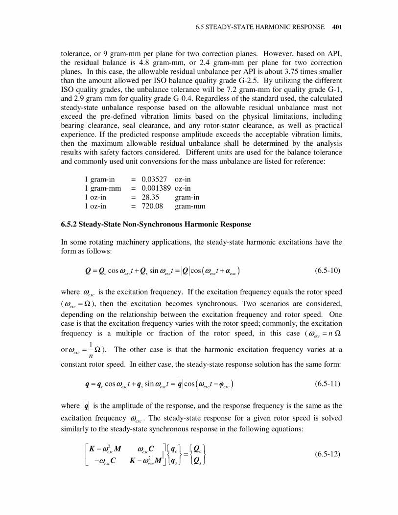
6.5 STEADY-STATE HARMONIC RESPONSE
401
tolerance, or 9 gram-mm per plane for two correction planes. However, based on API,
the residual balance is 4.8 gram-mm, or 2.4 gram-mm per plane for two correction
planes. In this case, the allowable residual unbalance per API is about 3.75 times smaller
than the amount allowed per ISO balance quality grade G-2.5. By utilizing the different
ISO quality grades, the unbalance tolerance will be 7.2 gram-mm for quality grade G-1,
and 2.9 gram-mm for quality grade G-0.4. Regardless of the standard used, the calculated
steady-state unbalance response based on the allowable residual unbalance must not
exceed the pre-defined vibration limits based on the physical limitations, including
bearing clearance, seal clearance, and any rotor-stator clearance, as well as practical
experience. If the predicted response amplitude exceeds the acceptable vibration limits,
then the maximum allowable residual unbalance shall be determined by the analysis
results with safety factors considered. Different units are used for the balance tolerance
and commonly used unit conversions for the mass unbalance are listed for reference:
1 gram-in = 0.03527 oz-in
1 gram-mm = 0.001389 oz-in
1 oz-in = 28.35 gram-in
1 oz-in = 720.08 gram-mm
6.5.2 Steady-State Non-Synchronous Harmonic Response
In some rotating machinery applications, the steady-state harmonic excitations have the
form as follows:
( )cos sin cosc exc s exc exc exc
t t tω ω ω= + = +Q Q Q Q α (6.5-10)
where exc
ω is the excitation frequency. If the excitation frequency equals the rotor speed
(exc
ω = Ω ), then the excitation becomes synchronous. Two scenarios are considered,
depending on the relationship between the excitation frequency and rotor speed. One
case is that the excitation frequency varies with the rotor speed; commonly, the excitation
frequency is a multiple or fraction of the rotor speed, in this case ( exc
nω = Ω
or1
excn
ω = Ω ). The other case is that the harmonic excitation frequency varies at a
constant rotor speed. In either case, the steady-state response solution has the same form:
( )cos sin cosc exc s exc exc exc
t t tω ω ω= + = −q q q q φ (6.5-11)
where q is the amplitude of the response, and the response frequency is the same as the
excitation frequency exc
ω . The steady-state response for a given rotor speed is solved
similarly to the steady-state synchronous response in the following equations:
2
2
c cexc exc
s sexc exc
ω ω
ω ω
− =
− −
q QK M C
q QC K M (6.5-12)
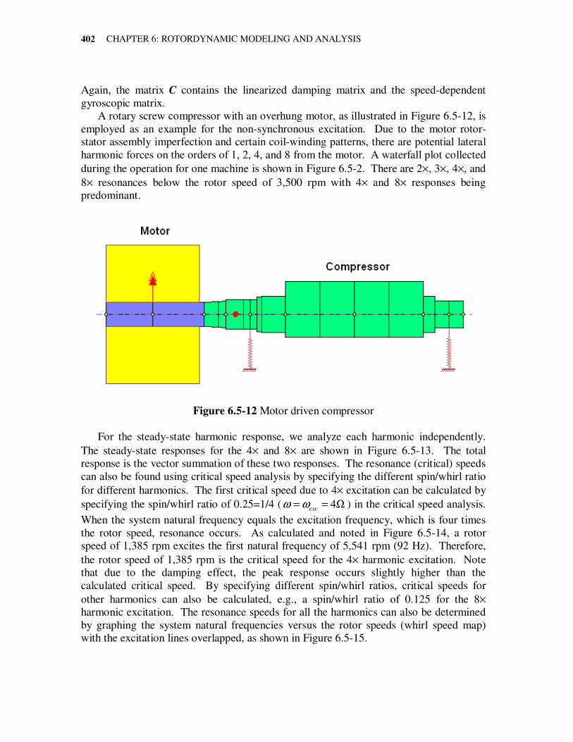
CHAPTER 6: ROTORDYNAMIC MODELING AND ANALYSIS
402
Again, the matrix C contains the linearized damping matrix and the speed-dependent
gyroscopic matrix.
A rotary screw compressor with an overhung motor, as illustrated in Figure 6.5-12, is
employed as an example for the non-synchronous excitation. Due to the motor rotor-
stator assembly imperfection and certain coil-winding patterns, there are potential lateral
harmonic forces on the orders of 1, 2, 4, and 8 from the motor. A waterfall plot collected
during the operation for one machine is shown in Figure 6.5-2. There are 2×, 3×, 4×, and
8× resonances below the rotor speed of 3,500 rpm with 4× and 8× responses being
predominant.
Figure 6.5-12 Motor driven compressor
For the steady-state harmonic response, we analyze each harmonic independently.
The steady-state responses for the 4× and 8× are shown in Figure 6.5-13. The total
response is the vector summation of these two responses. The resonance (critical) speeds
can also be found using critical speed analysis by specifying the different spin/whirl ratio
for different harmonics. The first critical speed due to 4× excitation can be calculated by
specifying the spin/whirl ratio of 0.25=1/4 ( 4exc
ω ω= = Ω ) in the critical speed analysis.
When the system natural frequency equals the excitation frequency, which is four times
the rotor speed, resonance occurs. As calculated and noted in Figure 6.5-14, a rotor
speed of 1,385 rpm excites the first natural frequency of 5,541 rpm (92 Hz). Therefore,
the rotor speed of 1,385 rpm is the critical speed for the 4× harmonic excitation. Note
that due to the damping effect, the peak response occurs slightly higher than the
calculated critical speed. By specifying different spin/whirl ratios, critical speeds for
other harmonics can also be calculated, e.g., a spin/whirl ratio of 0.125 for the 8×
harmonic excitation. The resonance speeds for all the harmonics can also be determined
by graphing the system natural frequencies versus the rotor speeds (whirl speed map)
with the excitation lines overlapped, as shown in Figure 6.5-15.
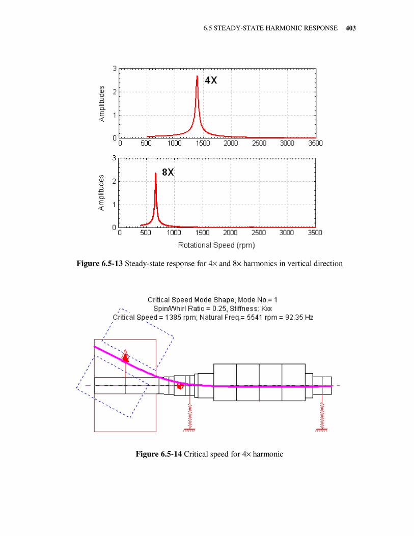
6.5 STEADY-STATE HARMONIC RESPONSE
403
Figure 6.5-13 Steady-state response for 4× and 8× harmonics in vertical direction
Figure 6.5-14 Critical speed for 4× harmonic
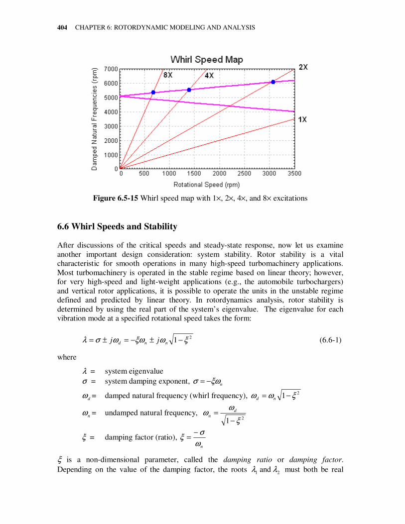
CHAPTER 6: ROTORDYNAMIC MODELING AND ANALYSIS
404
Figure 6.5-15 Whirl speed map with 1×, 2×, 4×, and 8× excitations
6.6 Whirl Speeds and Stability
After discussions of the critical speeds and steady-state response, now let us examine
another important design consideration: system stability. Rotor stability is a vital
characteristic for smooth operations in many high-speed turbomachinery applications.
Most turbomachinery is operated in the stable regime based on linear theory; however,
for very high-speed and light-weight applications (e.g., the automobile turbochargers)
and vertical rotor applications, it is possible to operate the units in the unstable regime
defined and predicted by linear theory. In rotordynamics analysis, rotor stability is
determined by using the real part of the system’s eigenvalue. The eigenvalue for each
vibration mode at a specified rotational speed takes the form:
2
1 ξωξωωσλ −±−=±= nnd jj (6.6-1)
where
λ = system eigenvalue
σ = system damping exponent, n
σ ξω= −
dω = damped natural frequency (whirl frequency), 2
1 ξωω −= nd
nω = undamped natural frequency, 21 ξ
ωω
−= d
n
ξ = damping factor (ratio), nω
σξ
−=
ξ is a non-dimensional parameter, called the damping ratio or damping factor.
Depending on the value of the damping factor, the roots 21 and λλ must both be real
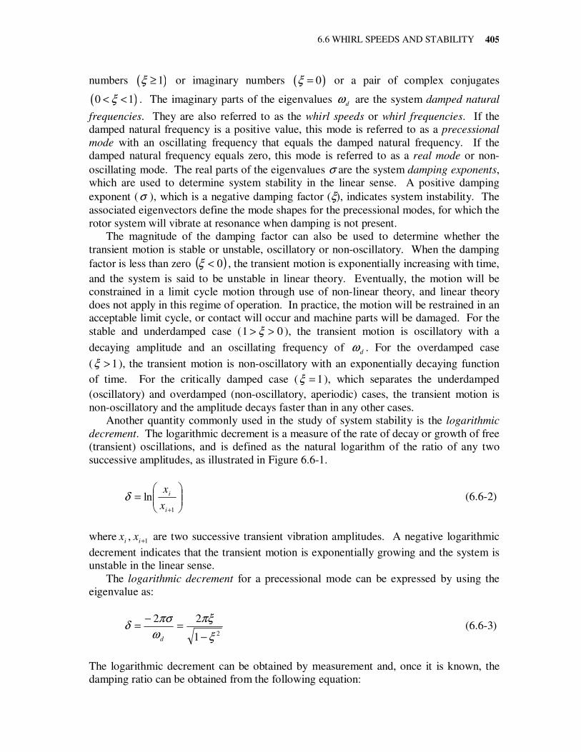
6.6 WHIRL SPEEDS AND STABILITY
405
numbers ( )1ξ ≥ or imaginary numbers ( )0ξ = or a pair of complex conjugates
( )0 1ξ< < . The imaginary parts of the eigenvalues dω are the system damped natural
frequencies. They are also referred to as the whirl speeds or whirl frequencies. If the
damped natural frequency is a positive value, this mode is referred to as a precessional
mode with an oscillating frequency that equals the damped natural frequency. If the
damped natural frequency equals zero, this mode is referred to as a real mode or non-
oscillating mode. The real parts of the eigenvalues σ are the system damping exponents,
which are used to determine system stability in the linear sense. A positive damping
exponent (σ ), which is a negative damping factor (ξ), indicates system instability. The
associated eigenvectors define the mode shapes for the precessional modes, for which the
rotor system will vibrate at resonance when damping is not present.
The magnitude of the damping factor can also be used to determine whether the
transient motion is stable or unstable, oscillatory or non-oscillatory. When the damping
factor is less than zero ( )0<ξ , the transient motion is exponentially increasing with time,
and the system is said to be unstable in linear theory. Eventually, the motion will be
constrained in a limit cycle motion through use of non-linear theory, and linear theory
does not apply in this regime of operation. In practice, the motion will be restrained in an
acceptable limit cycle, or contact will occur and machine parts will be damaged. For the
stable and underdamped case ( 01 >> ξ ), the transient motion is oscillatory with a
decaying amplitude and an oscillating frequency of dω . For the overdamped case
( 1>ξ ), the transient motion is non-oscillatory with an exponentially decaying function
of time. For the critically damped case ( 1=ξ ), which separates the underdamped
(oscillatory) and overdamped (non-oscillatory, aperiodic) cases, the transient motion is
non-oscillatory and the amplitude decays faster than in any other cases.
Another quantity commonly used in the study of system stability is the logarithmic
decrement. The logarithmic decrement is a measure of the rate of decay or growth of free
(transient) oscillations, and is defined as the natural logarithm of the ratio of any two
successive amplitudes, as illustrated in Figure 6.6-1.
=
+1
lni
i
x
xδ (6.6-2)
where 1 , +ii xx are two successive transient vibration amplitudes. A negative logarithmic
decrement indicates that the transient motion is exponentially growing and the system is
unstable in the linear sense.
The logarithmic decrement for a precessional mode can be expressed by using the
eigenvalue as:
21
22
ξ
πξ
ω
πσδ
−=
−=
d
(6.6-3)
The logarithmic decrement can be obtained by measurement and, once it is known, the
damping ratio can be obtained from the following equation:
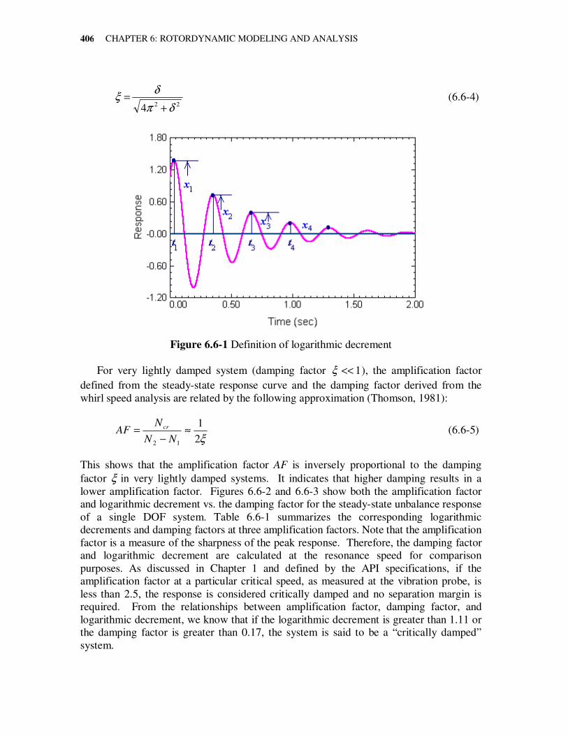
CHAPTER 6: ROTORDYNAMIC MODELING AND ANALYSIS
406
22
4 δπ
δξ
+= (6.6-4)
Figure 6.6-1 Definition of logarithmic decrement
For very lightly damped system (damping factor 1<<ξ ), the amplification factor
defined from the steady-state response curve and the damping factor derived from the
whirl speed analysis are related by the following approximation (Thomson, 1981):
ξ2
1
12
≈−
=NN
NAF cr (6.6-5)
This shows that the amplification factor AF is inversely proportional to the damping
factor ξ in very lightly damped systems. It indicates that higher damping results in a
lower amplification factor. Figures 6.6-2 and 6.6-3 show both the amplification factor
and logarithmic decrement vs. the damping factor for the steady-state unbalance response
of a single DOF system. Table 6.6-1 summarizes the corresponding logarithmic
decrements and damping factors at three amplification factors. Note that the amplification
factor is a measure of the sharpness of the peak response. Therefore, the damping factor
and logarithmic decrement are calculated at the resonance speed for comparison
purposes. As discussed in Chapter 1 and defined by the API specifications, if the
amplification factor at a particular critical speed, as measured at the vibration probe, is
less than 2.5, the response is considered critically damped and no separation margin is
required. From the relationships between amplification factor, damping factor, and
logarithmic decrement, we know that if the logarithmic decrement is greater than 1.11 or
the damping factor is greater than 0.17, the system is said to be a “critically damped”
system.
6.6 WHIRL SPEEDS AND STABILITY
407
Figure 6.6-2 Amplification factor vs. damping factor
Figure 6.6-3 Logarithmic decrement vs. damping factor
Table 6.6-1 Logarithmic decrements and damping factors at three amplification factors
Amplification Factor Damping Factor Logarithmic Decrement
2.5 0.17450 1.11350
5.0 0.09625 0.60758
8.0 0.06155 0.38746
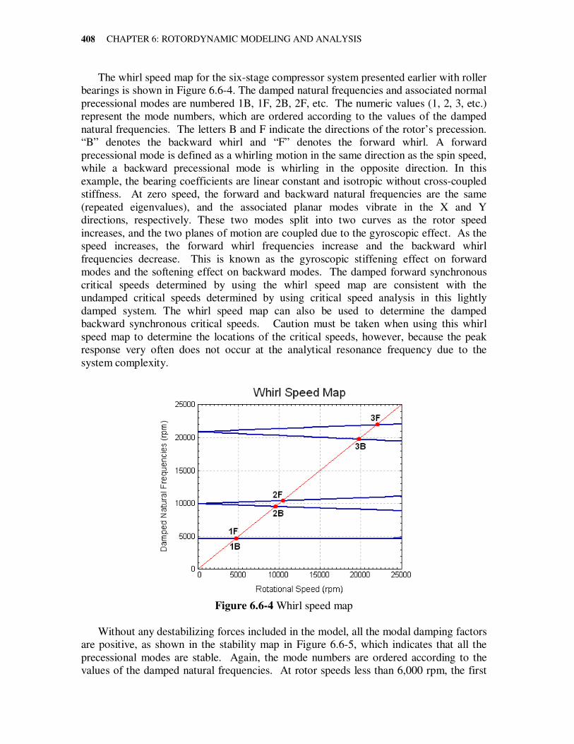
CHAPTER 6: ROTORDYNAMIC MODELING AND ANALYSIS
408
The whirl speed map for the six-stage compressor system presented earlier with roller
bearings is shown in Figure 6.6-4. The damped natural frequencies and associated normal
precessional modes are numbered 1B, 1F, 2B, 2F, etc. The numeric values (1, 2, 3, etc.)
represent the mode numbers, which are ordered according to the values of the damped
natural frequencies. The letters B and F indicate the directions of the rotor’s precession.
“B” denotes the backward whirl and “F” denotes the forward whirl. A forward
precessional mode is defined as a whirling motion in the same direction as the spin speed,
while a backward precessional mode is whirling in the opposite direction. In this
example, the bearing coefficients are linear constant and isotropic without cross-coupled
stiffness. At zero speed, the forward and backward natural frequencies are the same
(repeated eigenvalues), and the associated planar modes vibrate in the X and Y
directions, respectively. These two modes split into two curves as the rotor speed
increases, and the two planes of motion are coupled due to the gyroscopic effect. As the
speed increases, the forward whirl frequencies increase and the backward whirl
frequencies decrease. This is known as the gyroscopic stiffening effect on forward
modes and the softening effect on backward modes. The damped forward synchronous
critical speeds determined by using the whirl speed map are consistent with the
undamped critical speeds determined by using critical speed analysis in this lightly
damped system. The whirl speed map can also be used to determine the damped
backward synchronous critical speeds. Caution must be taken when using this whirl
speed map to determine the locations of the critical speeds, however, because the peak
response very often does not occur at the analytical resonance frequency due to the
system complexity.
Figure 6.6-4 Whirl speed map
Without any destabilizing forces included in the model, all the modal damping factors
are positive, as shown in the stability map in Figure 6.6-5, which indicates that all the
precessional modes are stable. Again, the mode numbers are ordered according to the
values of the damped natural frequencies. At rotor speeds less than 6,000 rpm, the first
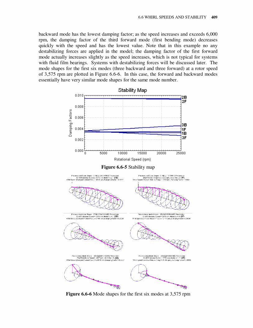
6.6 WHIRL SPEEDS AND STABILITY
409
backward mode has the lowest damping factor; as the speed increases and exceeds 6,000
rpm, the damping factor of the third forward mode (first bending mode) decreases
quickly with the speed and has the lowest value. Note that in this example no any
destabilizing forces are applied in the model; the damping factor of the first forward
mode actually increases slightly as the speed increases, which is not typical for systems
with fluid film bearings. Systems with destabilizing forces will be discussed later. The
mode shapes for the first six modes (three backward and three forward) at a rotor speed
of 3,575 rpm are plotted in Figure 6.6-6. In this case, the forward and backward modes
essentially have very similar mode shapes for the same mode number.
Figure 6.6-5 Stability map
Figure 6.6-6 Mode shapes for the first six modes at 3,575 rpm
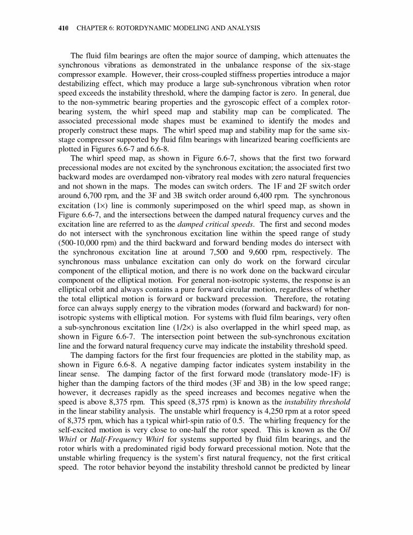
CHAPTER 6: ROTORDYNAMIC MODELING AND ANALYSIS
410
The fluid film bearings are often the major source of damping, which attenuates the
synchronous vibrations as demonstrated in the unbalance response of the six-stage
compressor example. However, their cross-coupled stiffness properties introduce a major
destabilizing effect, which may produce a large sub-synchronous vibration when rotor
speed exceeds the instability threshold, where the damping factor is zero. In general, due
to the non-symmetric bearing properties and the gyroscopic effect of a complex rotor-
bearing system, the whirl speed map and stability map can be complicated. The
associated precessional mode shapes must be examined to identify the modes and
properly construct these maps. The whirl speed map and stability map for the same six-
stage compressor supported by fluid film bearings with linearized bearing coefficients are
plotted in Figures 6.6-7 and 6.6-8.
The whirl speed map, as shown in Figure 6.6-7, shows that the first two forward
precessional modes are not excited by the synchronous excitation; the associated first two
backward modes are overdamped non-vibratory real modes with zero natural frequencies
and not shown in the maps. The modes can switch orders. The 1F and 2F switch order
around 6,700 rpm, and the 3F and 3B switch order around 6,400 rpm. The synchronous
excitation (1×) line is commonly superimposed on the whirl speed map, as shown in
Figure 6.6-7, and the intersections between the damped natural frequency curves and the
excitation line are referred to as the damped critical speeds. The first and second modes
do not intersect with the synchronous excitation line within the speed range of study
(500-10,000 rpm) and the third backward and forward bending modes do intersect with
the synchronous excitation line at around 7,500 and 9,600 rpm, respectively. The
synchronous mass unbalance excitation can only do work on the forward circular
component of the elliptical motion, and there is no work done on the backward circular
component of the elliptical motion. For general non-isotropic systems, the response is an
elliptical orbit and always contains a pure forward circular motion, regardless of whether
the total elliptical motion is forward or backward precession. Therefore, the rotating
force can always supply energy to the vibration modes (forward and backward) for non-
isotropic systems with elliptical motion. For systems with fluid film bearings, very often
a sub-synchronous excitation line (1/2×) is also overlapped in the whirl speed map, as
shown in Figure 6.6-7. The intersection point between the sub-synchronous excitation
line and the forward natural frequency curve may indicate the instability threshold speed.
The damping factors for the first four frequencies are plotted in the stability map, as
shown in Figure 6.6-8. A negative damping factor indicates system instability in the
linear sense. The damping factor of the first forward mode (translatory mode-1F) is
higher than the damping factors of the third modes (3F and 3B) in the low speed range;
however, it decreases rapidly as the speed increases and becomes negative when the
speed is above 8,375 rpm. This speed (8,375 rpm) is known as the instability threshold
in the linear stability analysis. The unstable whirl frequency is 4,250 rpm at a rotor speed
of 8,375 rpm, which has a typical whirl-spin ratio of 0.5. The whirling frequency for the
self-excited motion is very close to one-half the rotor speed. This is known as the Oil
Whirl or Half-Frequency Whirl for systems supported by fluid film bearings, and the
rotor whirls with a predominated rigid body forward precessional motion. Note that the
unstable whirling frequency is the system’s first natural frequency, not the first critical
speed. The rotor behavior beyond the instability threshold cannot be predicted by linear
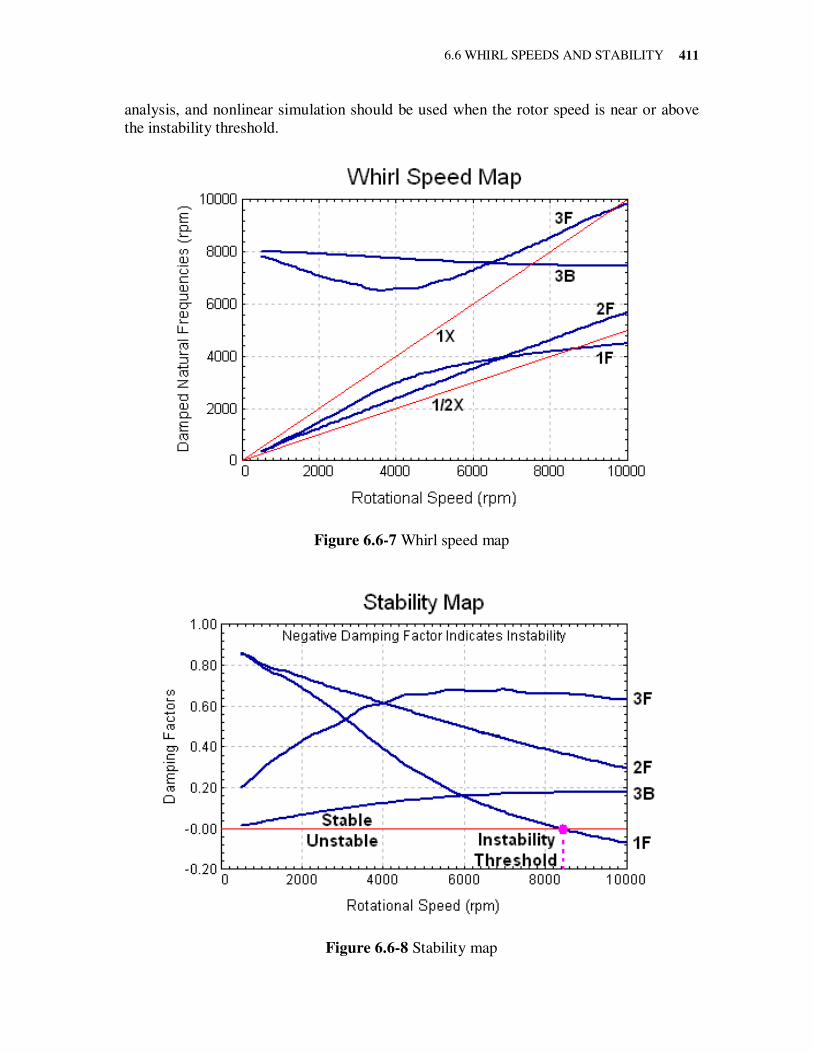
6.6 WHIRL SPEEDS AND STABILITY
411
analysis, and nonlinear simulation should be used when the rotor speed is near or above
the instability threshold.
Figure 6.6-7 Whirl speed map
Figure 6.6-8 Stability map
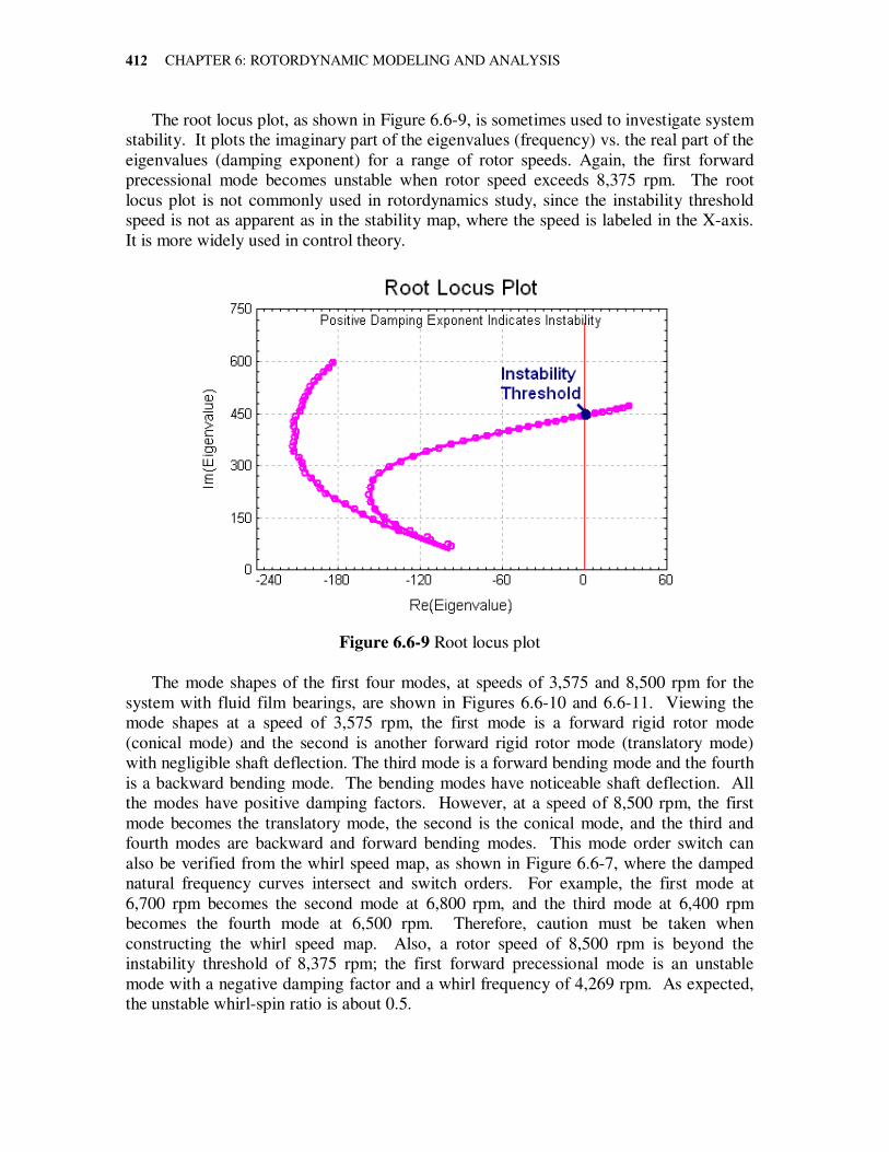
CHAPTER 6: ROTORDYNAMIC MODELING AND ANALYSIS
412
The root locus plot, as shown in Figure 6.6-9, is sometimes used to investigate system
stability. It plots the imaginary part of the eigenvalues (frequency) vs. the real part of the
eigenvalues (damping exponent) for a range of rotor speeds. Again, the first forward
precessional mode becomes unstable when rotor speed exceeds 8,375 rpm. The root
locus plot is not commonly used in rotordynamics study, since the instability threshold
speed is not as apparent as in the stability map, where the speed is labeled in the X-axis.
It is more widely used in control theory.
Figure 6.6-9 Root locus plot
The mode shapes of the first four modes, at speeds of 3,575 and 8,500 rpm for the
system with fluid film bearings, are shown in Figures 6.6-10 and 6.6-11. Viewing the
mode shapes at a speed of 3,575 rpm, the first mode is a forward rigid rotor mode
(conical mode) and the second is another forward rigid rotor mode (translatory mode)
with negligible shaft deflection. The third mode is a forward bending mode and the fourth
is a backward bending mode. The bending modes have noticeable shaft deflection. All
the modes have positive damping factors. However, at a speed of 8,500 rpm, the first
mode becomes the translatory mode, the second is the conical mode, and the third and
fourth modes are backward and forward bending modes. This mode order switch can
also be verified from the whirl speed map, as shown in Figure 6.6-7, where the damped
natural frequency curves intersect and switch orders. For example, the first mode at
6,700 rpm becomes the second mode at 6,800 rpm, and the third mode at 6,400 rpm
becomes the fourth mode at 6,500 rpm. Therefore, caution must be taken when
constructing the whirl speed map. Also, a rotor speed of 8,500 rpm is beyond the
instability threshold of 8,375 rpm; the first forward precessional mode is an unstable
mode with a negative damping factor and a whirl frequency of 4,269 rpm. As expected,
the unstable whirl-spin ratio is about 0.5.
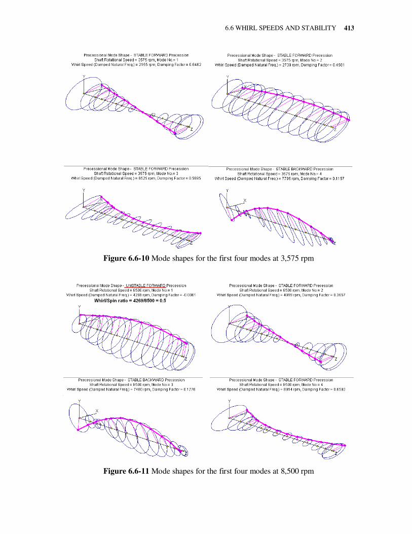
6.6 WHIRL SPEEDS AND STABILITY
413
Figure 6.6-10 Mode shapes for the first four modes at 3,575 rpm
Figure 6.6-11 Mode shapes for the first four modes at 8,500 rpm
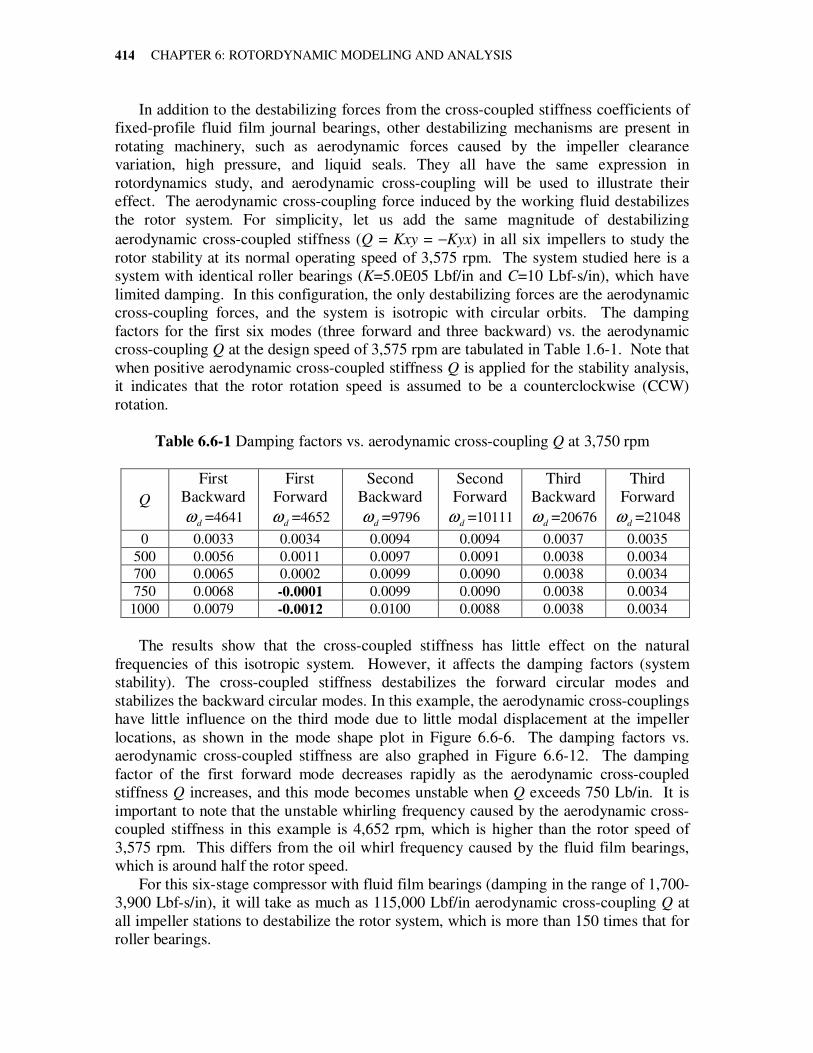
CHAPTER 6: ROTORDYNAMIC MODELING AND ANALYSIS
414
In addition to the destabilizing forces from the cross-coupled stiffness coefficients of
fixed-profile fluid film journal bearings, other destabilizing mechanisms are present in
rotating machinery, such as aerodynamic forces caused by the impeller clearance
variation, high pressure, and liquid seals. They all have the same expression in
rotordynamics study, and aerodynamic cross-coupling will be used to illustrate their
effect. The aerodynamic cross-coupling force induced by the working fluid destabilizes
the rotor system. For simplicity, let us add the same magnitude of destabilizing
aerodynamic cross-coupled stiffness (Q = Kxy = −Kyx) in all six impellers to study the
rotor stability at its normal operating speed of 3,575 rpm. The system studied here is a
system with identical roller bearings (K=5.0E05 Lbf/in and C=10 Lbf-s/in), which have
limited damping. In this configuration, the only destabilizing forces are the aerodynamic
cross-coupling forces, and the system is isotropic with circular orbits. The damping
factors for the first six modes (three forward and three backward) vs. the aerodynamic
cross-coupling Q at the design speed of 3,575 rpm are tabulated in Table 1.6-1. Note that
when positive aerodynamic cross-coupled stiffness Q is applied for the stability analysis,
it indicates that the rotor rotation speed is assumed to be a counterclockwise (CCW)
rotation.
Table 6.6-1 Damping factors vs. aerodynamic cross-coupling Q at 3,750 rpm
Q
First
Backward
dω =4641
First
Forward
dω =4652
Second
Backward
dω =9796
Second
Forward
dω =10111
Third
Backward
dω =20676
Third
Forward
dω =21048
0 0.0033 0.0034 0.0094 0.0094 0.0037 0.0035
500 0.0056 0.0011 0.0097 0.0091 0.0038 0.0034
700 0.0065 0.0002 0.0099 0.0090 0.0038 0.0034
750 0.0068 -0.0001 0.0099 0.0090 0.0038 0.0034
1000 0.0079 -0.0012 0.0100 0.0088 0.0038 0.0034
The results show that the cross-coupled stiffness has little effect on the natural
frequencies of this isotropic system. However, it affects the damping factors (system
stability). The cross-coupled stiffness destabilizes the forward circular modes and
stabilizes the backward circular modes. In this example, the aerodynamic cross-couplings
have little influence on the third mode due to little modal displacement at the impeller
locations, as shown in the mode shape plot in Figure 6.6-6. The damping factors vs.
aerodynamic cross-coupled stiffness are also graphed in Figure 6.6-12. The damping
factor of the first forward mode decreases rapidly as the aerodynamic cross-coupled
stiffness Q increases, and this mode becomes unstable when Q exceeds 750 Lb/in. It is
important to note that the unstable whirling frequency caused by the aerodynamic cross-
coupled stiffness in this example is 4,652 rpm, which is higher than the rotor speed of
3,575 rpm. This differs from the oil whirl frequency caused by the fluid film bearings,
which is around half the rotor speed.
For this six-stage compressor with fluid film bearings (damping in the range of 1,700-
3,900 Lbf-s/in), it will take as much as 115,000 Lbf/in aerodynamic cross-coupling Q at
all impeller stations to destabilize the rotor system, which is more than 150 times that for
roller bearings.
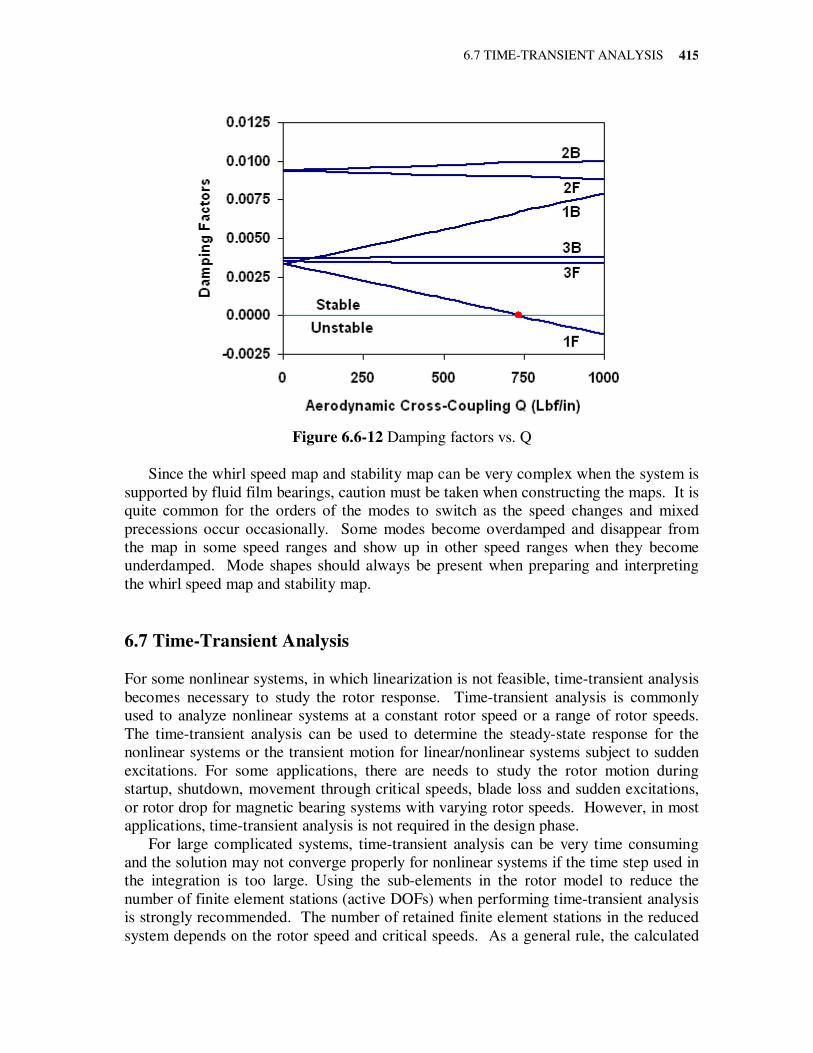
6.7 TIME-TRANSIENT ANALYSIS
415
Figure 6.6-12 Damping factors vs. Q
Since the whirl speed map and stability map can be very complex when the system is
supported by fluid film bearings, caution must be taken when constructing the maps. It is
quite common for the orders of the modes to switch as the speed changes and mixed
precessions occur occasionally. Some modes become overdamped and disappear from
the map in some speed ranges and show up in other speed ranges when they become
underdamped. Mode shapes should always be present when preparing and interpreting
the whirl speed map and stability map.
6.7 Time-Transient Analysis
For some nonlinear systems, in which linearization is not feasible, time-transient analysis
becomes necessary to study the rotor response. Time-transient analysis is commonly
used to analyze nonlinear systems at a constant rotor speed or a range of rotor speeds.
The time-transient analysis can be used to determine the steady-state response for the
nonlinear systems or the transient motion for linear/nonlinear systems subject to sudden
excitations. For some applications, there are needs to study the rotor motion during
startup, shutdown, movement through critical speeds, blade loss and sudden excitations,
or rotor drop for magnetic bearing systems with varying rotor speeds. However, in most
applications, time-transient analysis is not required in the design phase.
For large complicated systems, time-transient analysis can be very time consuming
and the solution may not converge properly for nonlinear systems if the time step used in
the integration is too large. Using the sub-elements in the rotor model to reduce the
number of finite element stations (active DOFs) when performing time-transient analysis
is strongly recommended. The number of retained finite element stations in the reduced
system depends on the rotor speed and critical speeds. As a general rule, the calculated
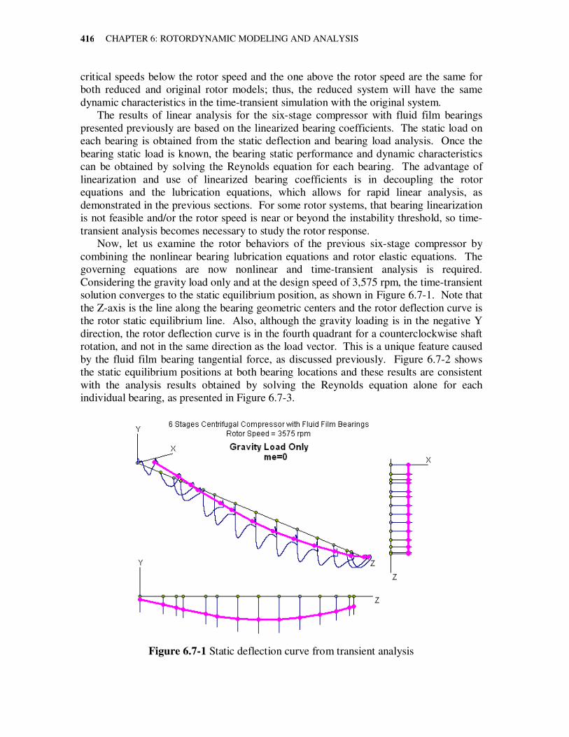
CHAPTER 6: ROTORDYNAMIC MODELING AND ANALYSIS
416
critical speeds below the rotor speed and the one above the rotor speed are the same for
both reduced and original rotor models; thus, the reduced system will have the same
dynamic characteristics in the time-transient simulation with the original system.
The results of linear analysis for the six-stage compressor with fluid film bearings
presented previously are based on the linearized bearing coefficients. The static load on
each bearing is obtained from the static deflection and bearing load analysis. Once the
bearing static load is known, the bearing static performance and dynamic characteristics
can be obtained by solving the Reynolds equation for each bearing. The advantage of
linearization and use of linearized bearing coefficients is in decoupling the rotor
equations and the lubrication equations, which allows for rapid linear analysis, as
demonstrated in the previous sections. For some rotor systems, that bearing linearization
is not feasible and/or the rotor speed is near or beyond the instability threshold, so time-
transient analysis becomes necessary to study the rotor response.
Now, let us examine the rotor behaviors of the previous six-stage compressor by
combining the nonlinear bearing lubrication equations and rotor elastic equations. The
governing equations are now nonlinear and time-transient analysis is required.
Considering the gravity load only and at the design speed of 3,575 rpm, the time-transient
solution converges to the static equilibrium position, as shown in Figure 6.7-1. Note that
the Z-axis is the line along the bearing geometric centers and the rotor deflection curve is
the rotor static equilibrium line. Also, although the gravity loading is in the negative Y
direction, the rotor deflection curve is in the fourth quadrant for a counterclockwise shaft
rotation, and not in the same direction as the load vector. This is a unique feature caused
by the fluid film bearing tangential force, as discussed previously. Figure 6.7-2 shows
the static equilibrium positions at both bearing locations and these results are consistent
with the analysis results obtained by solving the Reynolds equation alone for each
individual bearing, as presented in Figure 6.7-3.
Figure 6.7-1 Static deflection curve from transient analysis
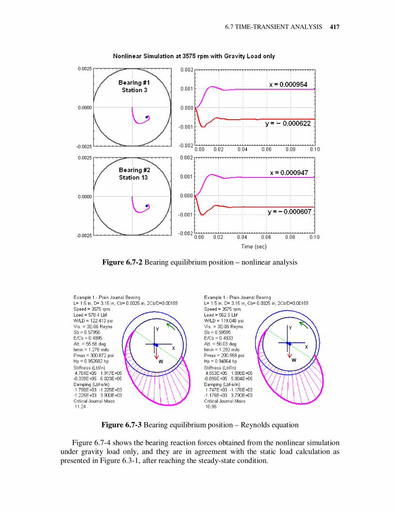
6.7 TIME-TRANSIENT ANALYSIS
417
Figure 6.7-2 Bearing equilibrium position – nonlinear analysis
Figure 6.7-3 Bearing equilibrium position – Reynolds equation
Figure 6.7-4 shows the bearing reaction forces obtained from the nonlinear simulation
under gravity load only, and they are in agreement with the static load calculation as
presented in Figure 6.3-1, after reaching the steady-state condition.
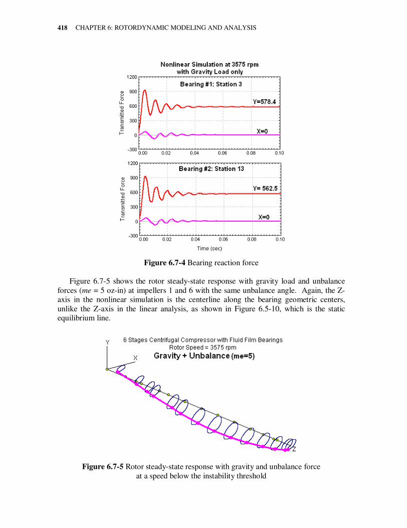
CHAPTER 6: ROTORDYNAMIC MODELING AND ANALYSIS
418
Figure 6.7-4 Bearing reaction force
Figure 6.7-5 shows the rotor steady-state response with gravity load and unbalance
forces (me = 5 oz-in) at impellers 1 and 6 with the same unbalance angle. Again, the Z-
axis in the nonlinear simulation is the centerline along the bearing geometric centers,
unlike the Z-axis in the linear analysis, as shown in Figure 6.5-10, which is the static
equilibrium line.
Figure 6.7-5 Rotor steady-state response with gravity and unbalance force
at a speed below the instability threshold
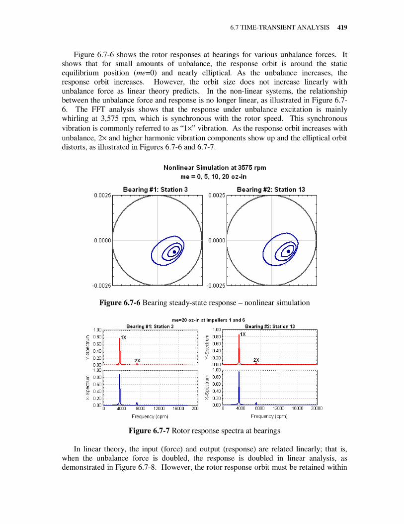
6.7 TIME-TRANSIENT ANALYSIS
419
Figure 6.7-6 shows the rotor responses at bearings for various unbalance forces. It
shows that for small amounts of unbalance, the response orbit is around the static
equilibrium position (me=0) and nearly elliptical. As the unbalance increases, the
response orbit increases. However, the orbit size does not increase linearly with
unbalance force as linear theory predicts. In the non-linear systems, the relationship
between the unbalance force and response is no longer linear, as illustrated in Figure 6.7-
6. The FFT analysis shows that the response under unbalance excitation is mainly
whirling at 3,575 rpm, which is synchronous with the rotor speed. This synchronous
vibration is commonly referred to as “1×” vibration. As the response orbit increases with
unbalance, 2× and higher harmonic vibration components show up and the elliptical orbit
distorts, as illustrated in Figures 6.7-6 and 6.7-7.
Figure 6.7-6 Bearing steady-state response – nonlinear simulation
Figure 6.7-7 Rotor response spectra at bearings
In linear theory, the input (force) and output (response) are related linearly; that is,
when the unbalance force is doubled, the response is doubled in linear analysis, as
demonstrated in Figure 6.7-8. However, the rotor response orbit must be retained within
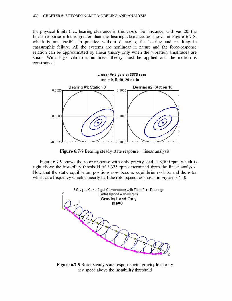
CHAPTER 6: ROTORDYNAMIC MODELING AND ANALYSIS
420
the physical limits (i.e., bearing clearance in this case). For instance, with me=20, the
linear response orbit is greater than the bearing clearance, as shown in Figure 6.7-8,
which is not feasible in practice without damaging the bearing and resulting in
catastrophic failure. All the systems are nonlinear in nature and the force-response
relation can be approximated by linear theory only when the vibration amplitudes are
small. With large vibration, nonlinear theory must be applied and the motion is
constrained.
Figure 6.7-8 Bearing steady-state response – linear analysis
Figure 6.7-9 shows the rotor response with only gravity load at 8,500 rpm, which is
right above the instability threshold of 8,375 rpm determined from the linear analysis.
Note that the static equilibrium positions now become equilibrium orbits, and the rotor
whirls at a frequency which is nearly half the rotor speed, as shown in Figure 6.7-10.
Figure 6.7-9 Rotor steady-state response with gravity load only
at a speed above the instability threshold
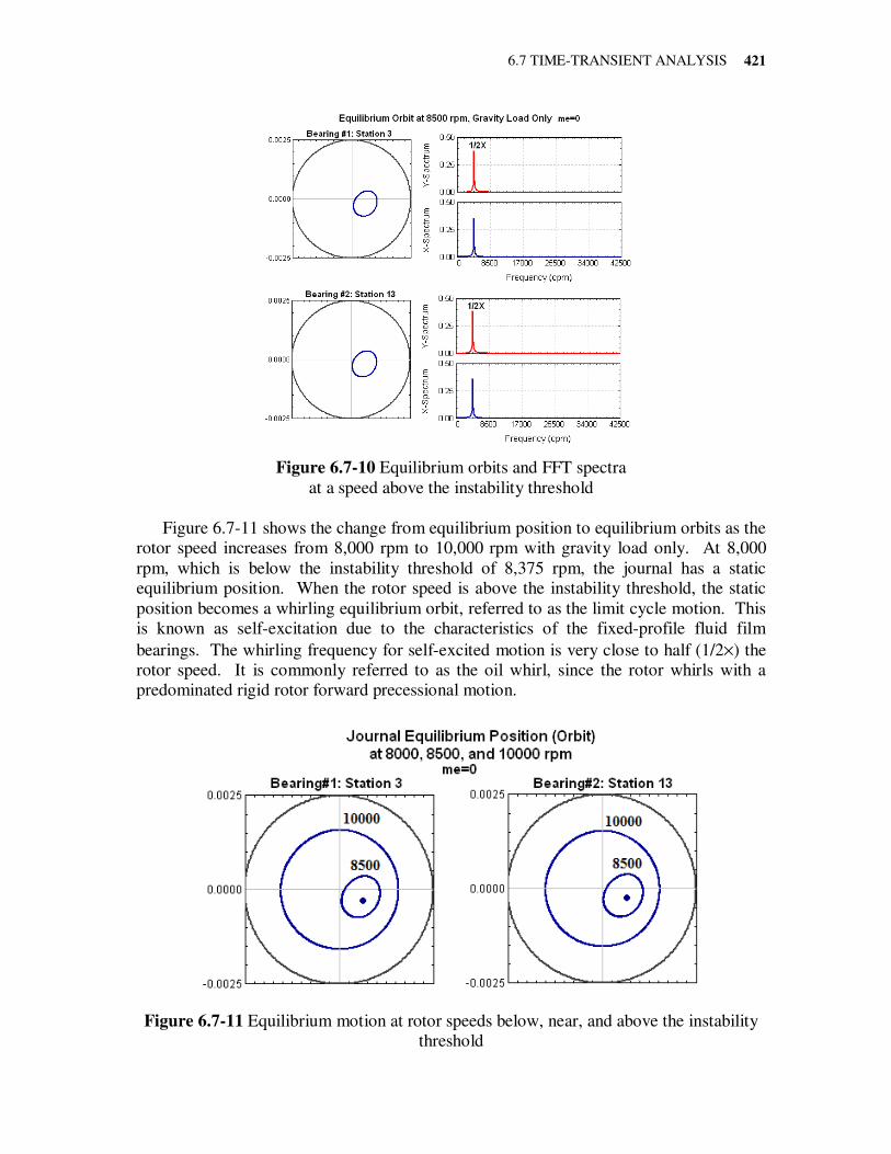
6.7 TIME-TRANSIENT ANALYSIS
421
Figure 6.7-10 Equilibrium orbits and FFT spectra
at a speed above the instability threshold
Figure 6.7-11 shows the change from equilibrium position to equilibrium orbits as the
rotor speed increases from 8,000 rpm to 10,000 rpm with gravity load only. At 8,000
rpm, which is below the instability threshold of 8,375 rpm, the journal has a static
equilibrium position. When the rotor speed is above the instability threshold, the static
position becomes a whirling equilibrium orbit, referred to as the limit cycle motion. This
is known as self-excitation due to the characteristics of the fixed-profile fluid film
bearings. The whirling frequency for self-excited motion is very close to half (1/2×) the
rotor speed. It is commonly referred to as the oil whirl, since the rotor whirls with a
predominated rigid rotor forward precessional motion.
Figure 6.7-11 Equilibrium motion at rotor speeds below, near, and above the instability
threshold
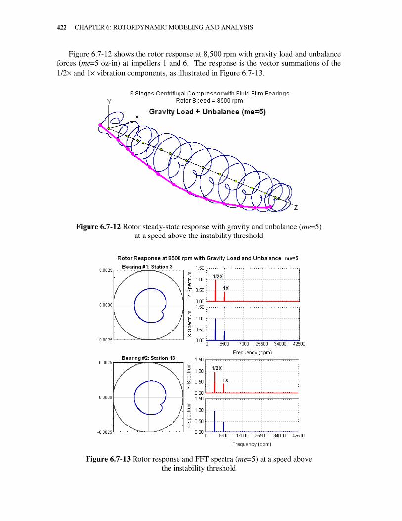
CHAPTER 6: ROTORDYNAMIC MODELING AND ANALYSIS
422
Figure 6.7-12 shows the rotor response at 8,500 rpm with gravity load and unbalance
forces (me=5 oz-in) at impellers 1 and 6. The response is the vector summations of the
1/2× and 1× vibration components, as illustrated in Figure 6.7-13.
Figure 6.7-12 Rotor steady-state response with gravity and unbalance (me=5)
at a speed above the instability threshold
Figure 6.7-13 Rotor response and FFT spectra (me=5) at a speed above
the instability threshold
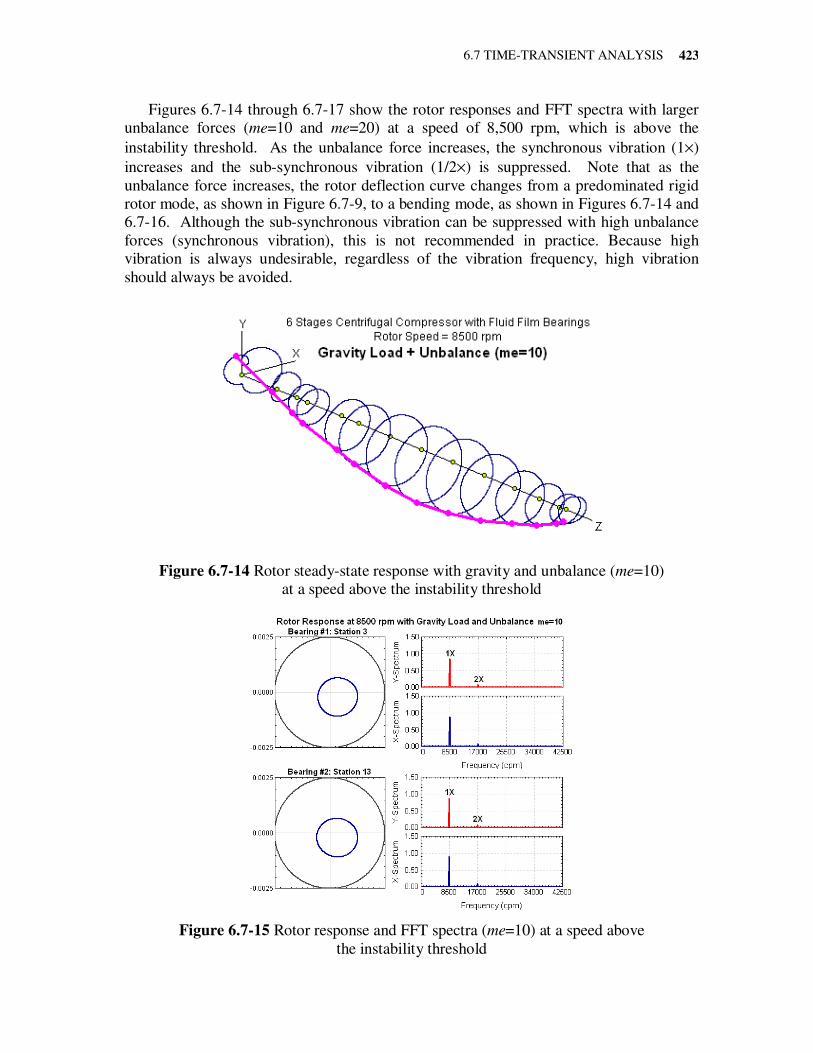
6.7 TIME-TRANSIENT ANALYSIS
423
Figures 6.7-14 through 6.7-17 show the rotor responses and FFT spectra with larger
unbalance forces (me=10 and me=20) at a speed of 8,500 rpm, which is above the
instability threshold. As the unbalance force increases, the synchronous vibration (1×)
increases and the sub-synchronous vibration (1/2×) is suppressed. Note that as the
unbalance force increases, the rotor deflection curve changes from a predominated rigid
rotor mode, as shown in Figure 6.7-9, to a bending mode, as shown in Figures 6.7-14 and
6.7-16. Although the sub-synchronous vibration can be suppressed with high unbalance
forces (synchronous vibration), this is not recommended in practice. Because high
vibration is always undesirable, regardless of the vibration frequency, high vibration
should always be avoided.
Figure 6.7-14 Rotor steady-state response with gravity and unbalance (me=10)
at a speed above the instability threshold
Figure 6.7-15 Rotor response and FFT spectra (me=10) at a speed above
the instability threshold
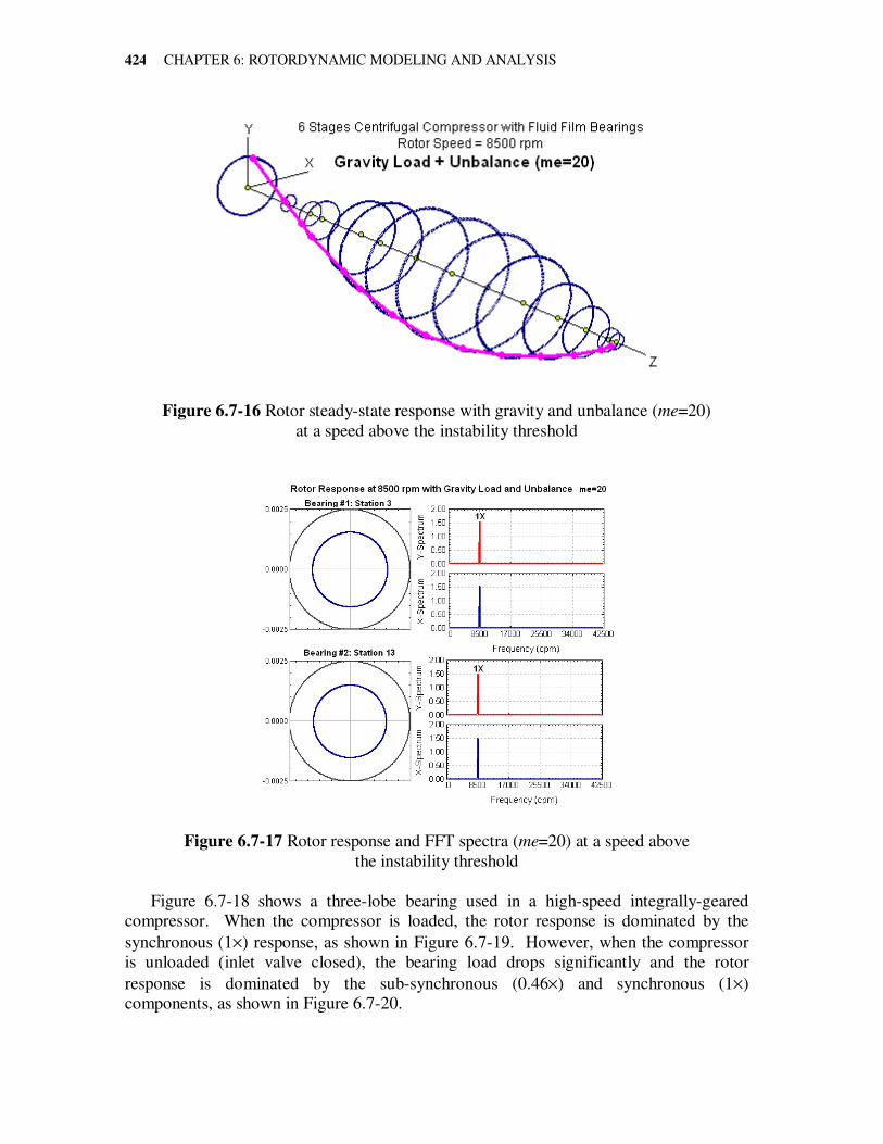
CHAPTER 6: ROTORDYNAMIC MODELING AND ANALYSIS
424
Figure 6.7-16 Rotor steady-state response with gravity and unbalance (me=20)
at a speed above the instability threshold
Figure 6.7-17 Rotor response and FFT spectra (me=20) at a speed above
the instability threshold
Figure 6.7-18 shows a three-lobe bearing used in a high-speed integrally-geared
compressor. When the compressor is loaded, the rotor response is dominated by the
synchronous (1×) response, as shown in Figure 6.7-19. However, when the compressor
is unloaded (inlet valve closed), the bearing load drops significantly and the rotor
response is dominated by the sub-synchronous (0.46×) and synchronous (1×)
components, as shown in Figure 6.7-20.
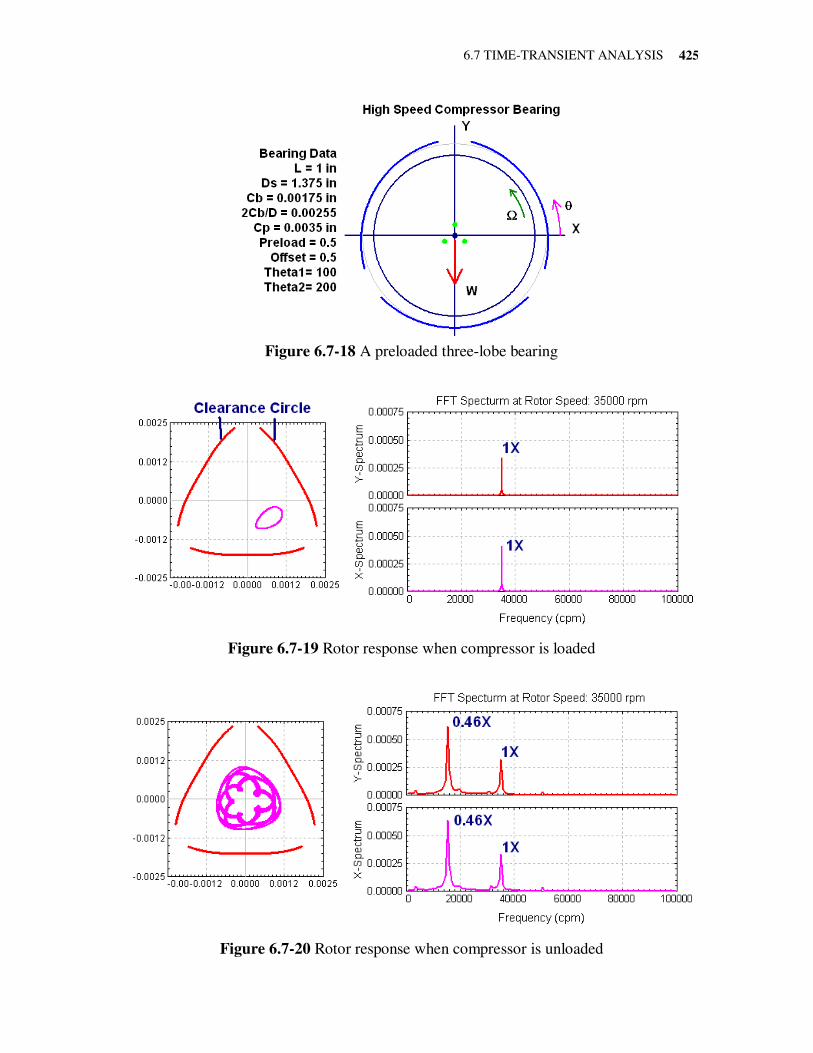
6.7 TIME-TRANSIENT ANALYSIS
425
Figure 6.7-18 A preloaded three-lobe bearing
Figure 6.7-19 Rotor response when compressor is loaded
Figure 6.7-20 Rotor response when compressor is unloaded
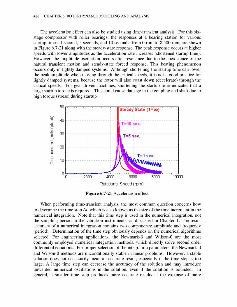
CHAPTER 6: ROTORDYNAMIC MODELING AND ANALYSIS
426
The acceleration effect can also be studied using time-transient analysis. For this six-
stage compressor with roller bearings, the responses at a bearing station for various
startup times, 1 second, 5 seconds, and 10 seconds, from 0 rpm to 8,500 rpm, are shown
in Figure 6.7-21 along with the steady-state response. The peak response occurs at higher
speeds with lower amplitudes as the acceleration rate increases (shortened startup time).
However, the amplitude oscillation occurs after resonance due to the coexistence of the
natural transient motion and steady-state forced response. This beating phenomenon
occurs only in lightly damped systems. Although shortening the startup time can lower
the peak amplitude when moving through the critical speeds, it is not a good practice for
lightly damped systems, because the rotor will also coast down (decelerate) through the
critical speeds. For gear-driven machines, shortening the startup time indicates that a
large startup torque is required. This could cause damage in the coupling and shaft due to
high torque (stress) during startup.
Figure 6.7-21 Acceleration effect
When performing time-transient analysis, the most common question concerns how
to determine the time step ∆t, which is also known as the size of the time increment in the
numerical integration. Note that this time step is used in the numerical integration, not
the sampling period in the vibration instruments, as discussed in Chapter 1. The result
accuracy of a numerical integration contains two components: amplitude and frequency
(period). Determination of the time step obviously depends on the numerical algorithms
selected. For engineering applications, the Newmark-β and Wilson-θ are the most
commonly employed numerical integration methods, which directly solve second order
differential equations. For proper selection of the integration parameters, the Newmark-β
and Wilson-θ methods are unconditionally stable in linear problems. However, a stable
solution does not necessarily mean an accurate result, especially if the time step is too
large. A large time step can decrease the accuracy of the solution and may introduce
unwanted numerical oscillations in the solution, even if the solution is bounded. In
general, a smaller time step produces more accurate results at the expense of more
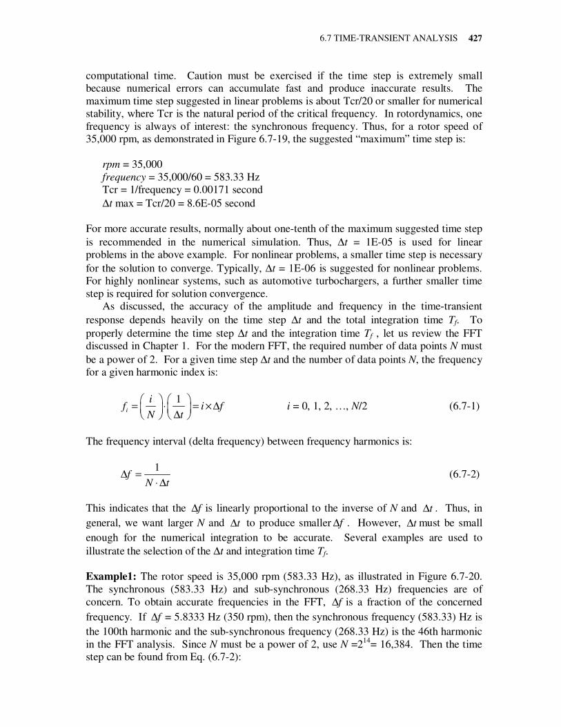
6.7 TIME-TRANSIENT ANALYSIS
427
computational time. Caution must be exercised if the time step is extremely small
because numerical errors can accumulate fast and produce inaccurate results. The
maximum time step suggested in linear problems is about Tcr/20 or smaller for numerical
stability, where Tcr is the natural period of the critical frequency. In rotordynamics, one
frequency is always of interest: the synchronous frequency. Thus, for a rotor speed of
35,000 rpm, as demonstrated in Figure 6.7-19, the suggested “maximum” time step is:
rpm = 35,000
frequency = 35,000/60 = 583.33 Hz
Tcr = 1/frequency = 0.00171 second
∆t max = Tcr/20 = 8.6E-05 second
For more accurate results, normally about one-tenth of the maximum suggested time step
is recommended in the numerical simulation. Thus, ∆t = 1E-05 is used for linear
problems in the above example. For nonlinear problems, a smaller time step is necessary
for the solution to converge. Typically, ∆t = 1E-06 is suggested for nonlinear problems.
For highly nonlinear systems, such as automotive turbochargers, a further smaller time
step is required for solution convergence.
As discussed, the accuracy of the amplitude and frequency in the time-transient
response depends heavily on the time step ∆t and the total integration time Tf. To
properly determine the time step ∆t and the integration time Tf , let us review the FFT
discussed in Chapter 1. For the modern FFT, the required number of data points N must
be a power of 2. For a given time step ∆t and the number of data points N, the frequency
for a given harmonic index is:
1
i
if i f
N t
= ⋅ = × ∆
∆ i = 0, 1, 2, …, N/2 (6.7-1)
The frequency interval (delta frequency) between frequency harmonics is:
1
fN t
∆ =⋅ ∆
(6.7-2)
This indicates that the f∆ is linearly proportional to the inverse of N and t∆ . Thus, in
general, we want larger N and t∆ to produce smaller f∆ . However, t∆ must be small
enough for the numerical integration to be accurate. Several examples are used to
illustrate the selection of the ∆t and integration time Tf.
Example1: The rotor speed is 35,000 rpm (583.33 Hz), as illustrated in Figure 6.7-20.
The synchronous (583.33 Hz) and sub-synchronous (268.33 Hz) frequencies are of
concern. To obtain accurate frequencies in the FFT, f∆ is a fraction of the concerned
frequency. If f∆ = 5.8333 Hz (350 rpm), then the synchronous frequency (583.33) Hz is
the 100th harmonic and the sub-synchronous frequency (268.33 Hz) is the 46th harmonic
in the FFT analysis. Since N must be a power of 2, use N =214
= 16,384. Then the time
step can be found from Eq. (6.7-2):
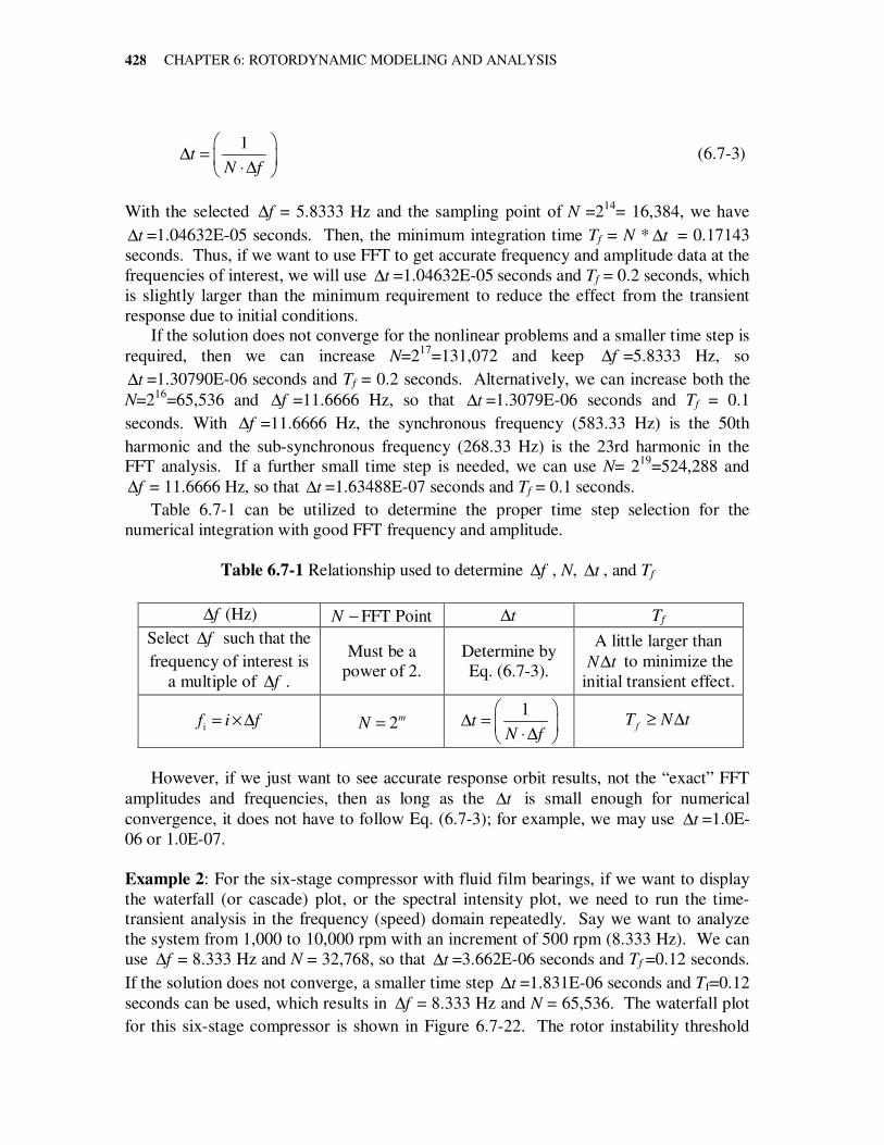
CHAPTER 6: ROTORDYNAMIC MODELING AND ANALYSIS
428
1
tN f
∆ =
⋅∆ (6.7-3)
With the selected f∆ = 5.8333 Hz and the sampling point of N =214
= 16,384, we have
t∆ =1.04632E-05 seconds. Then, the minimum integration time Tf = N * t∆ = 0.17143
seconds. Thus, if we want to use FFT to get accurate frequency and amplitude data at the
frequencies of interest, we will use t∆ =1.04632E-05 seconds and Tf = 0.2 seconds, which
is slightly larger than the minimum requirement to reduce the effect from the transient
response due to initial conditions.
If the solution does not converge for the nonlinear problems and a smaller time step is
required, then we can increase N=217
=131,072 and keep f∆ =5.8333 Hz, so
t∆ =1.30790E-06 seconds and Tf = 0.2 seconds. Alternatively, we can increase both the
N=216
=65,536 and f∆ =11.6666 Hz, so that t∆ =1.3079E-06 seconds and Tf = 0.1
seconds. With f∆ =11.6666 Hz, the synchronous frequency (583.33 Hz) is the 50th
harmonic and the sub-synchronous frequency (268.33 Hz) is the 23rd harmonic in the
FFT analysis. If a further small time step is needed, we can use N= 219
=524,288 and
f∆ = 11.6666 Hz, so that t∆ =1.63488E-07 seconds and Tf = 0.1 seconds.
Table 6.7-1 can be utilized to determine the proper time step selection for the
numerical integration with good FFT frequency and amplitude.
Table 6.7-1 Relationship used to determine f∆ , N, t∆ , and Tf
f∆ (Hz) N − FFT Point t∆ Tf
Select f∆ such that the
frequency of interest is
a multiple of f∆ .
Must be a
power of 2.
Determine by
Eq. (6.7-3).
A little larger than
N t∆ to minimize the
initial transient effect.
if i f= × ∆ 2mN = 1
tN f
∆ =
⋅∆ f
T N t≥ ∆
However, if we just want to see accurate response orbit results, not the “exact” FFT
amplitudes and frequencies, then as long as the t∆ is small enough for numerical
convergence, it does not have to follow Eq. (6.7-3); for example, we may use t∆ =1.0E-
06 or 1.0E-07.
Example 2: For the six-stage compressor with fluid film bearings, if we want to display
the waterfall (or cascade) plot, or the spectral intensity plot, we need to run the time-
transient analysis in the frequency (speed) domain repeatedly. Say we want to analyze
the system from 1,000 to 10,000 rpm with an increment of 500 rpm (8.333 Hz). We can
use f∆ = 8.333 Hz and N = 32,768, so that t∆ =3.662E-06 seconds and Tf =0.12 seconds.
If the solution does not converge, a smaller time step t∆ =1.831E-06 seconds and Tf=0.12
seconds can be used, which results in f∆ = 8.333 Hz and N = 65,536. The waterfall plot
for this six-stage compressor is shown in Figure 6.7-22. The rotor instability threshold
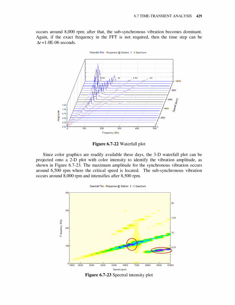
6.7 TIME-TRANSIENT ANALYSIS
429
occurs around 8,000 rpm; after that, the sub-synchronous vibration becomes dominant.
Again, if the exact frequency in the FFT is not required, then the time step can be
t∆ =1.0E-06 seconds.
Figure 6.7-22 Waterfall plot
Since color graphics are readily available these days, the 3-D waterfall plot can be
projected onto a 2-D plot with color intensity to identify the vibration amplitude, as
shown in Figure 6.7-23. The maximum amplitude for the synchronous vibration occurs
around 6,500 rpm where the critical speed is located. The sub-synchronous vibration
occurs around 8,000 rpm and intensifies after 8,500 rpm.
Figure 6.7-23 Spectral intensity plot
CHAPTER 6: ROTORDYNAMIC MODELING AND ANALYSIS
430
Example 3: To study the startup of an automotive turbocharger with floating ring
bearings, a frequency domain time-transient analysis is performed. The speed of interest
is from 15,000 to 200,000 rpm with an increment of 3,000 rpm (50 Hz). Since this is a
highly nonlinear system, the time step is very small, on the order of 1.0E-08 seconds, for
the numerical integration to converge. Let us use f∆ = 50 Hz to track the synchronous
vibration frequency. For the time step t∆ to be in the range of 1.0E-08, and the sampling
point N to be a power of 2, the number of FFT points is N=220
=1,048,576. Then,
1 1.90735 08(1048576 50)
t E∆ = = −×
seconds. The minimum integration time will be
1.90735 08 1048576 0.02f
T t N E= ∆ × = − × = seconds. With the same time step t∆ ,
increasing the integration time f
T will decrease the f∆ . Say, for example, doubling the
0.04f
T = will cut the 25f∆ = Hz in half.