THE INFLUENCE OF INTERNAL FRICTION ON ROTORDYNAMIC

INSTABILITY

A Thesis

by

ANAND SRINIVASAN

Submitted to the Office of Graduate Studies ofTexas A&M University

in partial fulfillment of the requirements for the degree of

MASTER OF SCIENCE

May 2003

Major Subject: Mechanical Engineering

THE INFLUENCE OF INTERNAL FRICTION ON ROTORDYNAMIC

INSTABILITY

A Thesis

by

ANAND SRINIVASAN

Submitted to Texas A&M Universityin partial fulfillment of the requirements

for the degree of

MASTER OF SCIENCE

Approved as to style and content by:

John M. Vance(Chair of Committee)

Luis San Andrés(Member)

Maurice Rahe(Member)

John Weese(Head of Department)

May 2003

Major Subject: Mechanical Engineering

iii

ABSTRACT

The Influence of Internal Friction on Rotordynamic Instability. (May 2003)

Anand Srinivasan, B.E., University of Madras

Chair of Advisory Committee: Dr. John M. Vance

Internal friction has been known to be a cause of whirl instability in built-up rotors since the

early 1900’s. This internal damping tends to make the rotor whirl at shaft speeds greater than a

critical speed, the whirl speed usually being equal to the critical speed. Over the years of

research, although models have been developed to explain instabilities due to internal friction, its

complex and unpredictable nature has made it extremely difficult to come up with a set of

equations or rules that can be used to predict instabilities accurate enough for design. This thesis

suggests improved methods for predicting the effects of shrink fits on threshold speeds of

instability. A supporting objective is to quantify the internal friction in the system by

measurements. Experimental methods of determining the internal damping with non-rotating

tests are investigated, and the results are correlated with appropriate mathematical models for the

system. Rotating experiments were carried out and suggest that subsynchronous vibration in

rotating machinery can have numerous sources or causes. Also, subsynchronous whirl due to

internal friction is not a highly repeatable phenomenon.

iv

DEDICATION

Amma

Appa

Engineering

v

ACKNOWLEDGMENTS

To Dr. John Vance for giving me an opportunity to work at the Turbomachinery Laboratory, for

teaching me the basics of rotordynamics and for inspiring me to the field.

To Dr. Luis San Andrés and Dr. Maurice Rahe for agreeing to be on my committee.

To Bharathwaj for his consistent support at A&M, no matter what happened.

To Arthur Picardo, Bugra Ertas and Eddie Denk for making me understand the fundamentals of

mechanical engineering.

To Avijit for helping me with XLTRC.

To Pradeep who taught me the meaning of the words Logic and Reasoning.

To my uncle Gopal, my chitti Jingla, my chitappa Krishnan, my brother Prabhu for their

encouragement and valuable advice.

To every friend and acquaintance of mine who has made this possible and who has been on my

side.

vi

NOMENCLATURE

cena = Acceleration of the center of the shaft

enda = Acceleration of the end of the shaft

Bd = Ball diameter

ic = Coefficient of internal damping

Modalc = Modal damping of the system

90C = Damping at 90 degree phase

D = Axial distance

F = Applied force

sF = Sampling rate

tanF = Tangential force due to whirling

h = Hysteretic damping coefficient

K = Stiffness of the system

)(dieqK = Equivalent stiffness of the disk

)(sheqK = Equivalent stiffness of the shaft

dm = Mass of the disk

sm = Mass of the shaft

)(sheqM = Equivalent mass of the shaft

cenm = Mass at the center of the shaft

endm = Mass at the end of the shaft

90M = Magnitude of the transfer function at 90 degree phase

eqeqeqeq FCKM ,,, = Equivalent mass, stiffness, damping, force of the 1 DOF system

Pd = Pitch diameter

r = Whirl radius

T = Taper ratio

vii

1X , 2X = Displacements of the masses

iZ = Normalized displacements

cenv = Velocity at the center of the shaft

endv = Velocity at the end of the shaft

bβ = Contact angle

δ = Logarithmic decrement

ω = Shaft rotative speed

crω = Critical speed of the system

dω = Damped natural frequency of the system

)(dinω = Natural frequency of the disk

•

φ = Whirl speed

F∆ = Frequency resolution

N = Number of samples

t∆ = Sampling period

ξ = Damping ratio

viii

TABLE OF CONTENTS

Page

ABSTRACT.............................................................................................................................iii

DEDICATION ......................................................................................................................... iv

ACKNOWLEDGMENTS ......................................................................................................... v

NOMENCLATURE ................................................................................................................. vi

TABLE OF CONTENTS........................................................................................................viii

LIST OF FIGURES................................................................................................................... x

CHAPTER I: INTRODUCTION ............................................................................................... 1

CHAPTER II: LITERATURE REVIEW.................................................................................... 3

CHAPTER III: BASICS OF INTERNAL ROTOR DAMPING.................................................. 6

Internal friction theory of shaft whirl................................................................................... 7

Procedure to determine internal damping ............................................................................ 9

CHAPTER IV: DESCRIPTION OF TEST RIG ....................................................................... 10

Adjusting the interference fit............................................................................................. 11

Parts of the test rig ............................................................................................................ 13

CHAPTER V: EFFECT OF FOUNDATION STIFFNESS ON THRESHOLD SPEED............ 14

Stiffening the foundation .................................................................................................. 14

Running tests .................................................................................................................... 17

Base case ...................................................................................................................... 17

Foundation stiffened on one end.................................................................................... 18

Foundation stiffened on both sides................................................................................. 18

Effect of balancing ........................................................................................................ 20

Addition of anti-seize compound................................................................................... 22

Hovering speed data...................................................................................................... 24

Tight fit......................................................................................................................... 26

Belt flapping constrained............................................................................................... 27

Tests with foundation stiffness asymmetry .................................................................... 29

Results for loose fit after tightening the bearing lock nut................................................ 30

Modeling using XLTRC2 ................................................................................................. 33

ix

Page

Discussion of results ......................................................................................................... 40

CHAPTER VI: QUANTIFYING INTERNAL FRICTION ...................................................... 43

Running tests .................................................................................................................... 43

Free vibration tests............................................................................................................ 45

Shaker tests ...................................................................................................................... 45

The disk-shaft system ....................................................................................................... 45

Modeling the disk-shaft system ..................................................................................... 45

Determination of the disk ( dm ) and the shaft ( sm ) masses ........................................... 48

Determination of modal mass ........................................................................................ 48

Determination of modal stiffness ................................................................................... 49

Determination of internal damping ................................................................................ 50

Analysis technique ........................................................................................................ 51

Results for the disk-shaft system without tape................................................................ 52

Results for the disk-shaft system with tape .................................................................... 54

Modeling of the disk-shaft system using XLTRC2 ........................................................ 58

Shaker tests of the shaft-only system................................................................................. 61

Modeling the shaft system ............................................................................................. 61

Determination of modal mass ........................................................................................ 61

Determination of modal stiffness ................................................................................... 62

Determination of internal damping ................................................................................ 62

Results for the shaft system ........................................................................................... 63

Experiments with wire stinger........................................................................................... 65

Discussion of shaker test results........................................................................................ 69

CHAPTER VII: SUMMARY AND FUTURE SCOPE ............................................................ 70

REFERENCES........................................................................................................................ 71

APPENDIX A ......................................................................................................................... 73

APPENDIX B ......................................................................................................................... 74

APPENDIX C ......................................................................................................................... 76

APPENDIX D ......................................................................................................................... 77

VITA....................................................................................................................................... 80

x

LIST OF FIGURES

Page

Figure 1: Model to explain shaft whirl due to internal friction .................................................... 8

Figure 2: Test rig ..................................................................................................................... 10

Figure 3: Taper sleeve.............................................................................................................. 11

Figure 4: Sleeve-shaft assembly............................................................................................... 12

Figure 5: Positions where the axial distance is measured .......................................................... 12

Figure 6: Arrangement to constrain the foundation................................................................... 15

Figure 7: Arrangement to measure the foundation stiffness ...................................................... 15

Figure 8: Force vs deflection curve for the foundation stiffness (case 1) ................................... 16

Figure 9: Force vs deflection curve for the foundation stiffness (3/8" cable) ............................. 17

Figure 10: Cascade plot of X probe for base case ..................................................................... 18

Figure 11: Cascade plot of X probe with one end of foundation stiffened ................................. 19

Figure 12: Cascade plot of X probe with both ends of foundation stiffened............................... 19

Figure 13: Waterfall plot of Y probe with balance mass added and foundation stiffened ........... 20

Figure 14: X probe frequency spectrum at 8960 rpm ................................................................ 21

Figure 15: X probe frequency spectrum at 5360 rpm ................................................................ 21

Figure 16: Y probe cascade plot with anti-seize applied and with balance mass ........................ 22

Figure 17: Y probe waterfall plot with anti-seize applied and with balance mass ...................... 23

Figure 18: Y probe cascade plot for machine hovering around 5700 rpm.................................. 23

Figure 19: Y probe waterfall plot for machine hovered around 5500 rpm ................................. 24

Figure 20: Y probe cascade plot for machine hovered around 5500 rpm for tight fit while

balanced ........................................................................................................................... 25

Figure 21: Y probe waterfall plot for machine hovered around 5500 rpm for tight fit while

balanced ........................................................................................................................... 25

Figure 22: Y probe cascade plot for machine hovering around 5500 rpm for tight fit without

balance screws.................................................................................................................. 26

Figure 23: Hardware arrangement to constrain the drive belt from flapping.............................. 27

Figure 24: Y probe cascade plot with belt flapping constrained ................................................ 28

Figure 25: Y probe waterfall plot with belt flapping constrained............................................... 28

xi

Page

Figure 26: Y probe waterfall plot without stiffening the foundation.......................................... 29

Figure 27: Lock nut that was tightened..................................................................................... 30

Figure 28: X probe waterfall plot with foundation constrained after lock nut was tightened ...... 31

Figure 29: Orbit of 0.5X filtered component at 5200 rpm ......................................................... 31

Figure 30: X probe cascade plot for tight fit with foundation constrained after tightening luck

nut .................................................................................................................................... 32

Figure 31: X probe cascade plot for tight fit without constraining foundation after tightening

luck nut ............................................................................................................................ 32

Figure 32: Frequency spectrum at 5300 rpm............................................................................. 33

Figure 33: Model of the rotor-bearing system........................................................................... 34

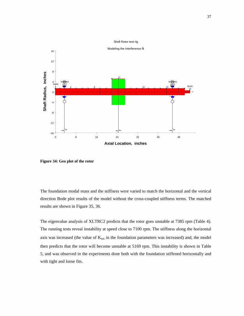
Figure 34: Geo plot of the rotor................................................................................................ 37

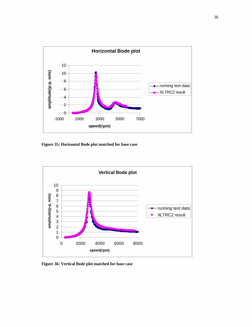
Figure 35: Horizontal Bode plot matched for base case ............................................................ 38

Figure 36: Vertical Bode plot matched for base case ................................................................ 38

Figure 37: Waterfall plot for the system with tape, low interference ......................................... 44

Figure 38: Waterfall plot for the system with tape, high interference ........................................ 44

Figure 39: Motion of the disk-shaft system when hung free-free............................................... 46

Figure 40: 2 DOF model of disk-shaft system and the equivalent 1 DOF model ....................... 46

Figure 41: Mode shape of the disk-shaft system ....................................................................... 49

Figure 42: Set-up arrangement ................................................................................................. 51

Figure 43: Loose fit with tape on both sides ............................................................................. 55

Figure 44: Tight fit with tape on both sides .............................................................................. 55

Figure 45: Loose fit with no tape.............................................................................................. 56

Figure 46: Tight fit with no tape............................................................................................... 56

Figure 47: Damping comparison for 90 degree method ............................................................ 57

Figure 48: LabVIEW verification............................................................................................. 57

Figure 49: Shaft shaken with the standard stinger..................................................................... 64

Figure 50 : Spectrum of force transducer.................................................................................. 64

Figure 51: Shaker test with the wire stinger.............................................................................. 65

Figure 52: Mass calibration curve ............................................................................................ 66

Figure 53 : Spectrum of force transducer with wire stinger....................................................... 67

xii

Page

Figure 54: Cross-coupled stiffness representing a destabilizing force........................................ 76

xiii

LIST OF TABLES

Page

Table 1 : Ball bearing spread sheet XLBALBRG ..................................................................... 35

Table 2: Foundation parameters spread sheet XLUSEKCM ..................................................... 35

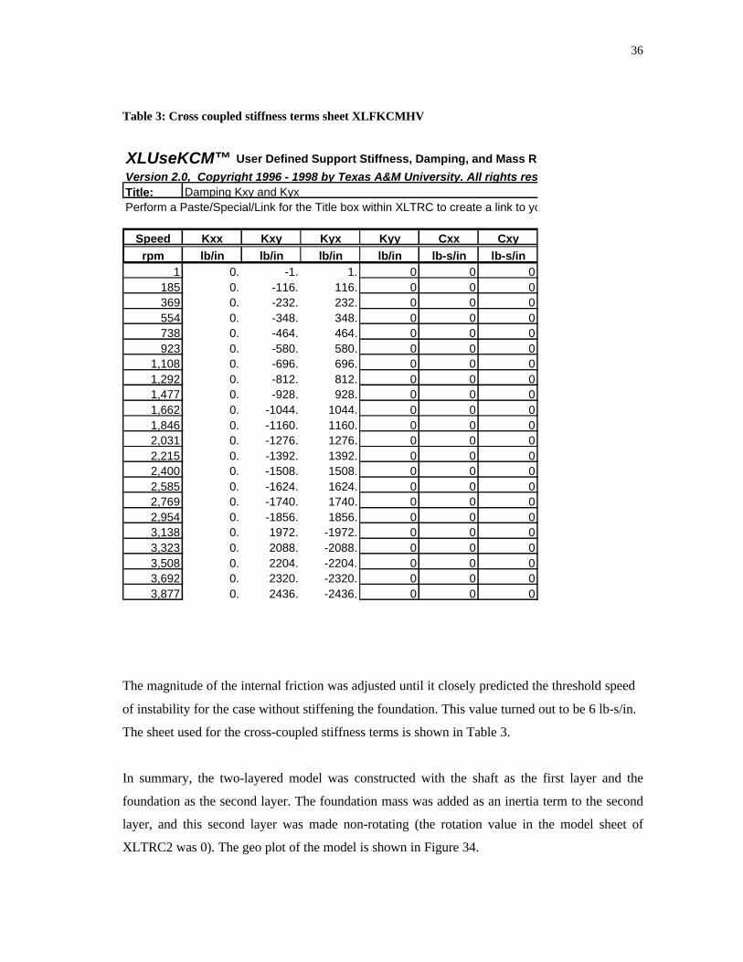
Table 3: Cross coupled stiffness terms sheet XLFKCMHV ...................................................... 36

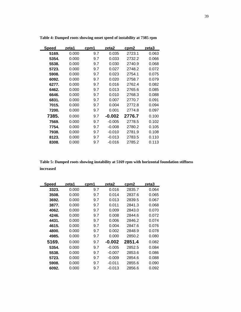
Table 4: Damped roots showing onset speed of instability at 7385 rpm .................................... 39

Table 5: Damped roots showing instability at 5169 rpm with horizontal foundation stiffness

increased .......................................................................................................................... 39

Table 6: Extract from Mir's thesis showing the logarithmic decrement values of the free-

free tests ........................................................................................................................... 53

Table 7: Modal parameters for disk-shaft system with standard stinger..................................... 54

Table 8: Cross-coupled stiffness terms to represent the actual damping in the system ............... 59

Table 9: Eigenvalue for the free-free case showing the damping ratio....................................... 59

Table 10: Damping values used in XLTRC2 to match the damping ratio .................................. 60

Table 11: Damping ratios obtained from plugging in damping values at the disk-shaft

interface............................................................................................................................ 60

Table 12: Eigenvalues for case with tape.................................................................................. 60

Table 13 : Modal parameters for shaft with standard stinger ..................................................... 63

Table 14 : Modal parameters for shaft with wire stinger ........................................................... 67

Table 15 : Modal parameters for disk-shaft with wire stinger ................................................... 68

Table 16 : Comparison of tests done with the two types of stingers for the disk-shaft system.... 68

1

CHAPTER I

INTRODUCTION

A recurring problem in rotordynamics is the whirl instability caused by internal friction in a

built-up rotor. Though this friction dampens and suppresses the amplitude of free vibrations

when the rotor is non-rotating, the friction induces self-excited vibrations at high rotor speeds

and causes the amplitude of vibrations to increase until it reaches a limit cycle or until it causes

destruction to the system; this is termed as rotordynamic instability.

In rotating systems, friction or damping is classified into two categories. The first category is

damping in non-rotating parts, and is called external damping or external friction. Examples are

bearing damping and air drag, which stabilize the system. The second category is internal

friction, which acts in the rotating parts, and drives the rotor unstable at speeds above the critical

speed. Though past researchers have modeled the internal friction as viscous, recent analyses and

experiments show that internal friction is dominantly hysteretic rather than viscous.

The instability caused by internal friction causes the rotor to begin to whirl at shaft speeds

greater than the critical speed. The whirl frequency is usually equal to a critical speed of the

rotor. In most cases, the whirl instability can be suppressed with hardware fixes such as changing

the bearings to softer supports with asymmetric stiffness, adding more external damping or

tightening the interference fits. However, predicting the threshold speed of instability in built-up

rotors at the design stage still remains a challenge, since quantifying internal friction numerically

is a difficult task. Hence the need arises to develop a suitable model to predict the characteristics

of built-up rotors at high speeds.

This thesis follows the style and format of the ASME Journal of Turbomachinery.

2

The objectives of this research are:

1. To develop an improved capability to predict the threshold speed of instability in built-up

rotors with shrink and other types of interference joints.

2. To measure subsynchronous vibrations from various sources and to classify them as benign

or potentially unstable, thus providing a diagnostic tool.

3. To study the effect of foundation stiffness and rotor imbalance on the onset speed of

instability due to internal friction.

4. To explore experimental methods of quantifying internal friction in rotors.

3

CHAPTER II

LITERATURE REVIEW

The design philosophy applied to rotating machinery initially began with the construction of

very stiff rotors that would ensure operation below the first critical speed. It was only after

Jeffcott’s [1] analysis in 1919, when he showed that rotors could be made to run beyond the first

critical speed with proper rotor balancing that the trend in rotordynamics design changed. As the

rigid rotor model was replaced by the more flexible one, several failures were encountered when

operating at speeds above the first critical speed. Most of the failures were of unknown origin at

that time. Newkirk [2] of General Electric Research Laboratory investigated the failures of

compressor units in 1924, and found that these units encountered violent whirling at speeds

above the first critical, with the whirling rate being equal to the first critical speed. If the rotor

speed were increased above its initial whirl speed, the whirl amplitude would increase, leading to

rotor failure. The speed at which the rotor begins to whirl is the onset speed of instability.

Kimball [3], working with Newkirk, suggested internal friction to be the cause of shaft whirling.

He showed that below the first critical speed, the internal friction would damp out the whirl

motion, while above the critical speed, it would sustain the whirl.

After a series of experiments, Newkirk and Kimball arrived at a number of conclusions, the most

important being: the onset speed of whirling or the whirl amplitude is unaffected by rotor

balance, whirling always occurs above the first critical, whirling is encountered only in built-up

rotors, increasing the foundation flexibility or increasing the damping to the foundation increases

the whirl threshold speed.

In 1964, Ehrich [4] conducted an analysis of the instability induced by internal damping in a

rotor and showed that the induced whirl need not necessarily excite the fundamental mode and

that for various damping conditions a particular mode would be excited. He showed that in

general, whirling occurs in the mode whose whirl speed is approximately one half of the

rotational speed.

4

Gunter [5] in 1967 provided a theoretical explanation to Newkirk’s findings. He modeled a

flexible rotor on elastic supports and was able to come up with an analytical expression to

predict the onset speed of instability. He was able to prove that rotor balance has no effect on the

stability. He also proved that decreasing the foundation stiffness increased the threshold speed of

whirl instability.

In 1969, Gunter and Trumpler [6] showed that in the absence of bearing damping a symmetric

flexible foundation would reduce the rotor critical speed and also the whirl threshold speed.

They also showed that if external damping was added, the threshold speed could be greatly

improved. They also showed that foundation asymmetry without foundation damping can cause

a large increase of the onset speed of instability.

Begg [7] in 1976 conducted a stability analysis due to friction induced whirl for a simple flexible

rotor and showed that there exists regimes of stability, depending on the stiffness and damping

characteristics. Begg computed a stability chart to determine whether a disturbance would decay,

grow or remain bounded during or after removal of the disturbance.

Vance and Lee [8] in 1973 did a mathematical analysis to determine the threshold speed of

instability of non-synchronous whirl for an unbalanced flexible rotor on a rigid foundation. They

proved that the threshold speed is the same for balanced and unbalanced rotors. They concluded

that rotors can operated safely up to speeds about eighty percent above the significant critical

speed if external damping is larger than internal friction, and that shaft stiffness orthotropy has

an insignificant effect on friction-induced whirl.

Black [9] in 1976 used a hysteretic model to predict that there would be a finite speed range of

whirl instability, which could be passed through safely. Ying and Vance [10] verified this in

1994 by performing tests on a built-up rotor. The internal friction was found to vary with

temperature and the tightness of fit. The amount of damping of the rotor on bearings could not be

accurately found since the bearing stiffness varied with the angular position of the shaft.

Bently and Muszynska [11] (1985) were able to produce self excited vibrations on a shaft by

covering it with a 4-mil thick layer of damping material commonly used for vibration control

5

(acrylic adhesive, ISD-112). They were able to prove that the damping material increased the

internal friction on the shaft.

Lund [12] in 1986 studied the destabilizing forces due to internal friction using viscous,

coulomb, hysteretic and micro-slip models. He compared them based on the energy input to the

whirl motion, and developed conditions for instability due to internal friction in a micro-slip.

Parker [13] (1997) and Vance (1996) developed a procedure to measure the internal friction of a

built-up rotor. The rotor was freely suspended and excited with a shaker. It was found that the

first mode on bearings could be approximated with the free-free mode shape by adding extra

masses to the ends of the rotor. The logarithmic decrement could then be found and converted to

an equivalent viscous and hysteretic damping coefficient, which could be used in rotordynamic

codes to predict the instability. The rule of thumb that Parker came up with for the mass to be

added to the end of the rotor was that the mass should be twice the weight of the rotor. This

requirement makes the procedure impractical for heavy rotors.

Bently [14] in 1972 revisited Kimball’s 1924 papers and showed that internal friction produces

forward whirl with circular orbits, thus driving the system unstable.

Mir and Khalid [15], [16] (2001) showed that the measure of the logarithmic decrement from

free-free rap tests of the shrink fit rotor could give a measure of the internal damping. They

showed that internal friction is amplitude dependent. They performed rotating tests, which

showed that the rotor would go unstable at high speeds, and modeled the rotor-bearing system

with XLTRC, a computer code, in an attempt to predict the threshold speed. Their foundation

model used synchronous force coefficients.

6

CHAPTER III

BASICS OF INTERNAL ROTOR DAMPING

Friction is generated between any two bodies in contact with each other, moving or tending to

move in opposite directions. Damping, a more general term, is the process by which the

amplitude of vibration steadily decreases [17]. The energy is dissipated in the form of friction or

heat. The various forms of damping are viscous, coulomb and hysteretic damping.

Viscous damping arises from fluid interaction, in which the damping is proportional to the

velocity. In a viscously damped harmonic motion, the successive amplitudes have a logarithmic

relation with one another. The viscous damping can be found from the logarithmic decrement.

Coulomb or dry friction damping is caused due to the kinetic energy dissipated between sliding

surfaces. Hysteresis or solid damping is caused by the internal friction when a solid is deformed,

and is independent of frequency.

In rotating systems, external friction or damping tends to stabilize the system. Internal damping

in rotors is destabilizing. It can be generated by the different layers of the material tending to

slide across each other when the shaft rotates. The energy dissipated over a cycle in viscous

damping is frequency dependent (increases with increase in frequency). A viscous damping

model is not an accurate representation of internal damping.

The energy dissipated in a hysteretic model is frequency independent or slightly decreases with

increasing frequency and is a more realistic representation of the internal damping. The internal

hysteretic damping can be represented by assuming the damping force to be directly proportional

to the velocity and inversely proportional to the frequency. The constant h that is replaced by

ωic is called the hysteretic constant [17].

ih c ω= Eq 3. 1

Hysteretic damping can be converted to logarithmic decrement using Eqn 3.2.

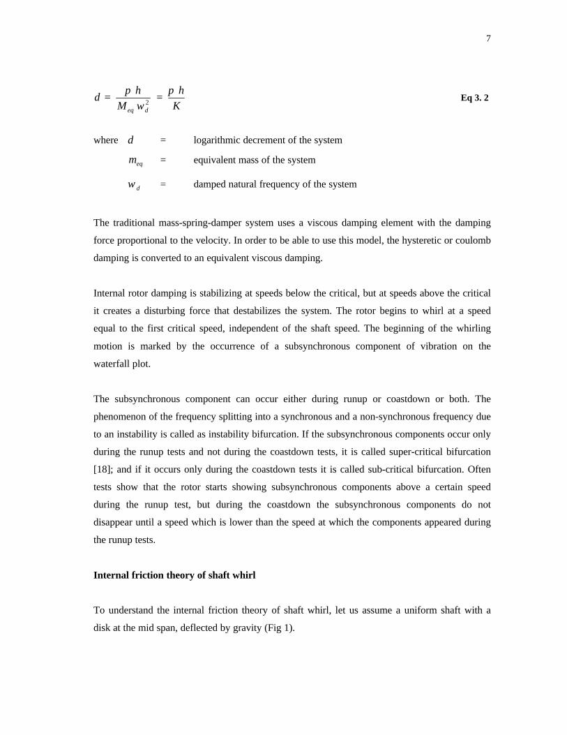
7

2eq d

h h

M K

π πδ

ω= = Eq 3. 2

where δ = logarithmic decrement of the system

eqm = equivalent mass of the system

dω = damped natural frequency of the system

The traditional mass-spring-damper system uses a viscous damping element with the damping

force proportional to the velocity. In order to be able to use this model, the hysteretic or coulomb

damping is converted to an equivalent viscous damping.

Internal rotor damping is stabilizing at speeds below the critical, but at speeds above the critical

it creates a disturbing force that destabilizes the system. The rotor begins to whirl at a speed

equal to the first critical speed, independent of the shaft speed. The beginning of the whirling

motion is marked by the occurrence of a subsynchronous component of vibration on the

waterfall plot.

The subsynchronous component can occur either during runup or coastdown or both. The

phenomenon of the frequency splitting into a synchronous and a non-synchronous frequency due

to an instability is called as instability bifurcation. If the subsynchronous components occur only

during the runup tests and not during the coastdown tests, it is called super-critical bifurcation

[18]; and if it occurs only during the coastdown tests it is called sub-critical bifurcation. Often

tests show that the rotor starts showing subsynchronous components above a certain speed

during the runup test, but during the coastdown the subsynchronous components do not

disappear until a speed which is lower than the speed at which the components appeared during

the runup tests.

Internal friction theory of shaft whirl

To understand the internal friction theory of shaft whirl, let us assume a uniform shaft with a

disk at the mid span, deflected by gravity (Fig 1).

8

W/2 W/2

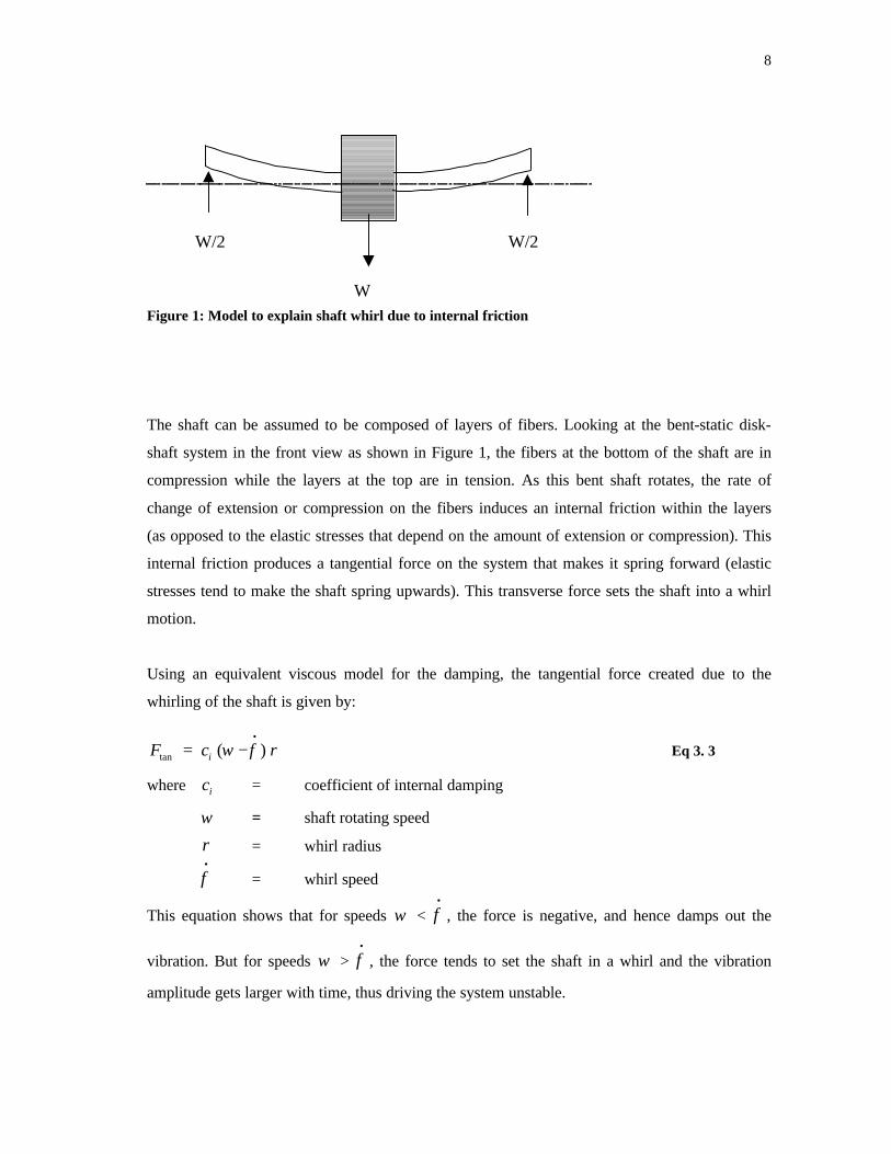
WFigure 1: Model to explain shaft whirl due to internal friction

The shaft can be assumed to be composed of layers of fibers. Looking at the bent-static disk-

shaft system in the front view as shown in Figure 1, the fibers at the bottom of the shaft are in

compression while the layers at the top are in tension. As this bent shaft rotates, the rate of

change of extension or compression on the fibers induces an internal friction within the layers

(as opposed to the elastic stresses that depend on the amount of extension or compression). This

internal friction produces a tangential force on the system that makes it spring forward (elastic

stresses tend to make the shaft spring upwards). This transverse force sets the shaft into a whirl

motion.

Using an equivalent viscous model for the damping, the tangential force created due to the

whirling of the shaft is given by:

tan ( )iF c rω φ•

= − Eq 3. 3

where ic = coefficient of internal damping

ω = shaft rotating speed

r = whirl radius•

φ = whirl speed

This equation shows that for speeds ω < •

φ , the force is negative, and hence damps out the

vibration. But for speeds ω > •

φ , the force tends to set the shaft in a whirl and the vibration

amplitude gets larger with time, thus driving the system unstable.

9

The natural whirling speed of the system of the system is the damped natural frequency dω . For

light external damping, dω will approximately be equal to the critical speed of the system crω .

Hence the destabilizing tangential force can be written as

tan ( )i crF c rω ω= − Eq 3. 4

Procedure to determine internal damping

Internal damping in a system can be determined by hanging the rotor free-free and rapping to get

the logarithmic decrement of the system. Mir [16] and Khalid [15] had done rap tests on the

disk-shaft system studied here and had determined the logarithmic decrement from which an

equivalent viscous damping was determined. One of the concerns in a rap test is to simulate the

running speed peak amplitude and the only way of doing this is to rap the rotor hard enough so

that the peak due to the impulsive force of the hammer is comparable with the running speed

peak amplitude.

In order to simulate the running speed amplitudes in a static test, a shaker, capable of exerting

about 30 lb force over a range of frequencies is a good alternative to the rap tests. Hence a shaker

was used in this thesis to excite the rotor, and parameter identification was carried out by

analyzing the frequency response of dynamic stiffness transfer functions ( XF / ). Models were

developed and the validity of the test results was confirmed by correlating the results with the

mathematical model and the XLTRC2 model.

10

CHAPTER IV

DESCRIPTION OF TEST RIG

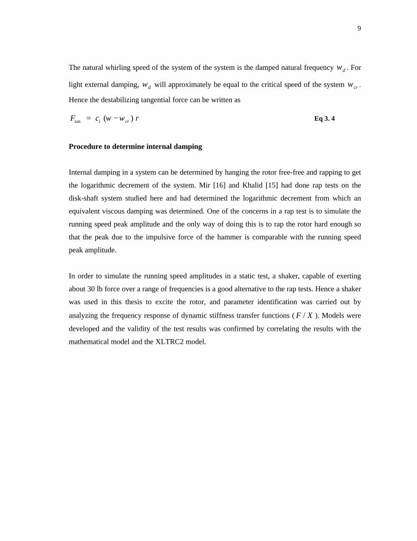
The test rig donated by Shell Oil Co. (Figure 2.) was used for the experiments.

Figure 2: Test rig

A single disk rotor with a taper sleeve arrangement was used to vary the interference fit. The

rotor assembly weighs 79.5 kg (175 lb) and is 1.32 m (52.25”) long. The shaft diameter is 63.5

mm (2.5”). The wheel diameter is 254 mm (10”) and is 127 mm (5”) long. The wheel resides at

the center of the shaft. The shaft is supported on ball bearings; the bearing span is 1.07 m (42”).

11

1.1505.060

1.210

4.550

SLEEVE TAPER TO BE24:1 ON THE DIAMETER

±0.001

2.700 2.530

±0.001

2.500

5.000

2.9

080

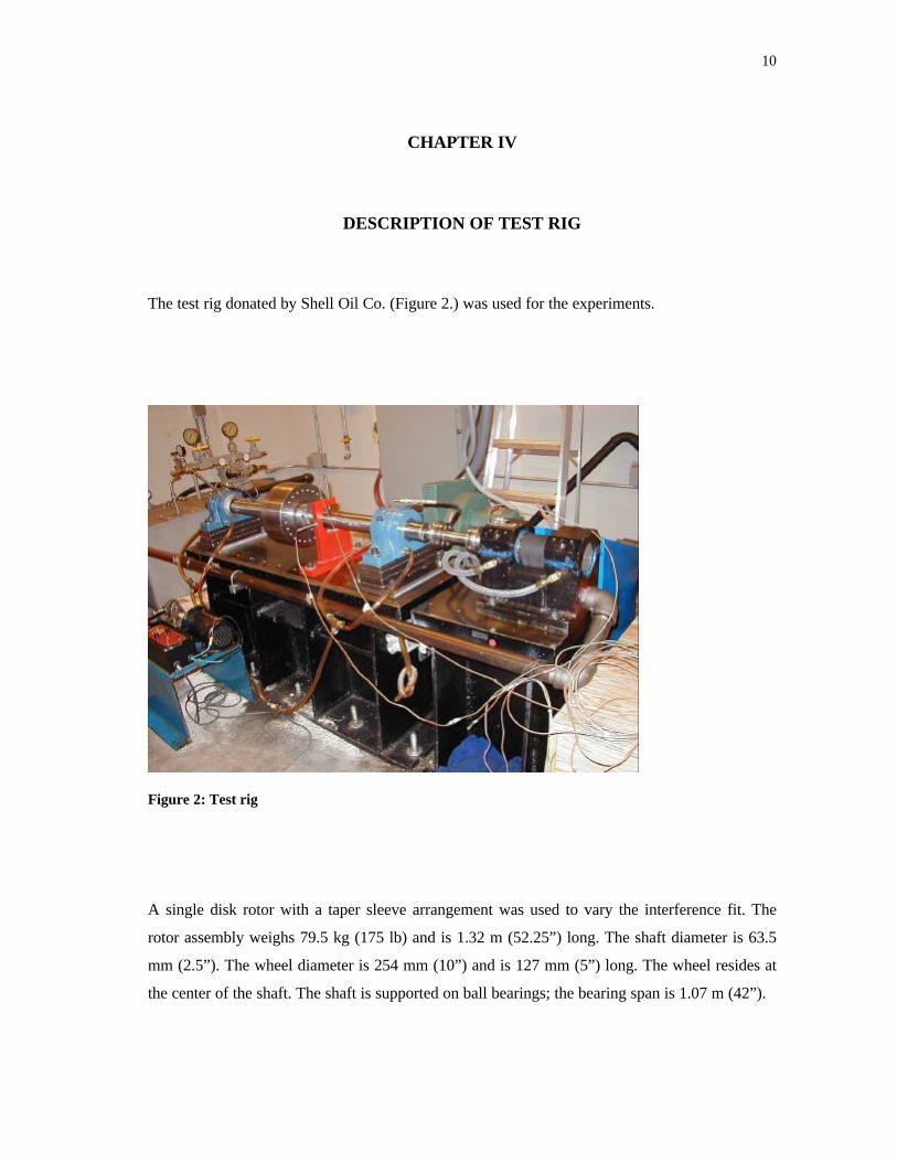
Figure 3: Taper sleeve

Adjusting the interference fit

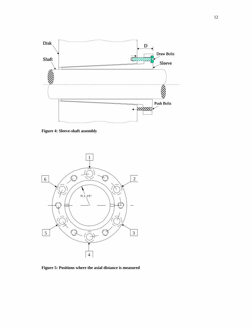
The taper sleeve arrangement is shown in Figure 3. The taper in the sleeve is 1/24. The disk is

mounted on the tapered portion of the sleeve. The Allen bolts that connect the sleeve and the

disk are used to vary the interference between the two elements. These bolts are arranged equi-

spaced along the periphery of the sleeve; there are a total of 12 bolts. The fit can be made more

or less tight by tightening or loosening the draw and the push bolts that are shown in Figure 4. A

measure of the interference is given in terms of D, denoted in Figure 4. From the geometry of the

disk, the distance D that gives zero interference is 39.1668 mm (1.542”), and is denoted by S.

The formula to calculate the radial interference is

( )DST

If −=2

Eq 4. 1

12

D Disk

Shaft Sleeve

Push Bolts

Draw Bolts

D Disk

Shaft Sleeve

Push Bolts

Draw Bolts

Figure 4: Sleeve-shaft assembly

R 1.25"

2

1

3

4

5

6

Figure 5: Positions where the axial distance is measured

13

where T is the taper ratio and is 1/24. Substituting these values in the equation, we get the

following equations.

( )DIfEnglish −⋅= 542.102083.0 inches

( )DIf SI −⋅= 1668.3902083.0 mm

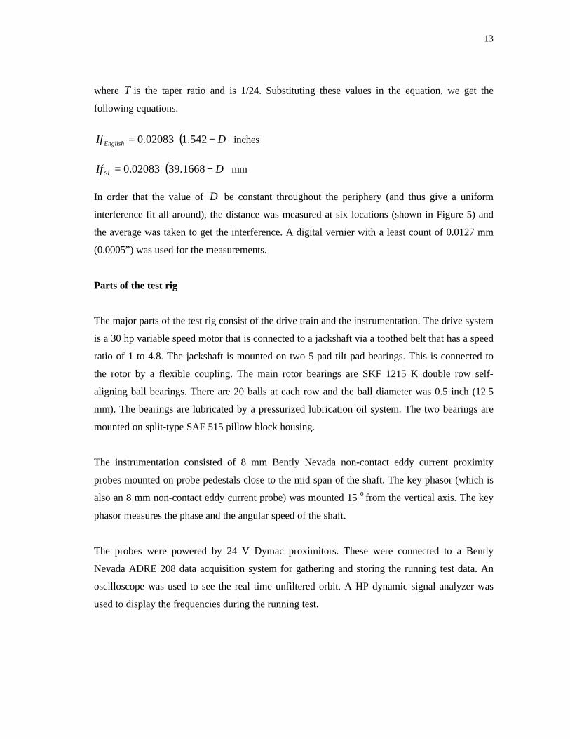
In order that the value of D be constant throughout the periphery (and thus give a uniform

interference fit all around), the distance was measured at six locations (shown in Figure 5) and

the average was taken to get the interference. A digital vernier with a least count of 0.0127 mm

(0.0005”) was used for the measurements.

Parts of the test rig

The major parts of the test rig consist of the drive train and the instrumentation. The drive system

is a 30 hp variable speed motor that is connected to a jackshaft via a toothed belt that has a speed

ratio of 1 to 4.8. The jackshaft is mounted on two 5-pad tilt pad bearings. This is connected to

the rotor by a flexible coupling. The main rotor bearings are SKF 1215 K double row self-

aligning ball bearings. There are 20 balls at each row and the ball diameter was 0.5 inch (12.5

mm). The bearings are lubricated by a pressurized lubrication oil system. The two bearings are

mounted on split-type SAF 515 pillow block housing.

The instrumentation consisted of 8 mm Bently Nevada non-contact eddy current proximity

probes mounted on probe pedestals close to the mid span of the shaft. The key phasor (which is

also an 8 mm non-contact eddy current probe) was mounted 15 0 from the vertical axis. The key

phasor measures the phase and the angular speed of the shaft.

The probes were powered by 24 V Dymac proximitors. These were connected to a Bently

Nevada ADRE 208 data acquisition system for gathering and storing the running test data. An

oscilloscope was used to see the real time unfiltered orbit. A HP dynamic signal analyzer was

used to display the frequencies during the running test.

14

CHAPTER V

EFFECT OF FOUNDATION STIFFNESS ON THRESHOLD SPEED

Literature [5] shows that the onset speed of instability (OSI) depends on the foundation stiffness;

the OSI is lower for a foundation with symmetric stiffness along the horizontal and the vertical

directions, as compared to an asymmetric one. One objective of this thesis is to study the effect

of increase in the horizontal stiffness of the foundation (thus making it more symmetric) on the

OSI due to internal friction. Another objective is to differentiate benign from potentially unstable

subsynchronous vibrations. Ferrara [19], working with high speed compressor units, has

suggested that subsynchronous vibration does not always indicate instability. This chapter

enumerates experiments done by stiffening the foundation horizontally. Rap tests previously

done by Mir [16] and Khalid [15] showed that the horizontal and vertical natural frequencies are

40 Hz and 52 Hz. They also showed that at some values of low interference fit, the system

became unstable at high speeds, while no instability was noted for tighter fits.

Stiffening the foundation

In this thesis, the word “foundation” refers to the welded steel structure supporting the bearing

housing. It is anchor bolted to the concrete floor. To study the effect of increase in the horizontal

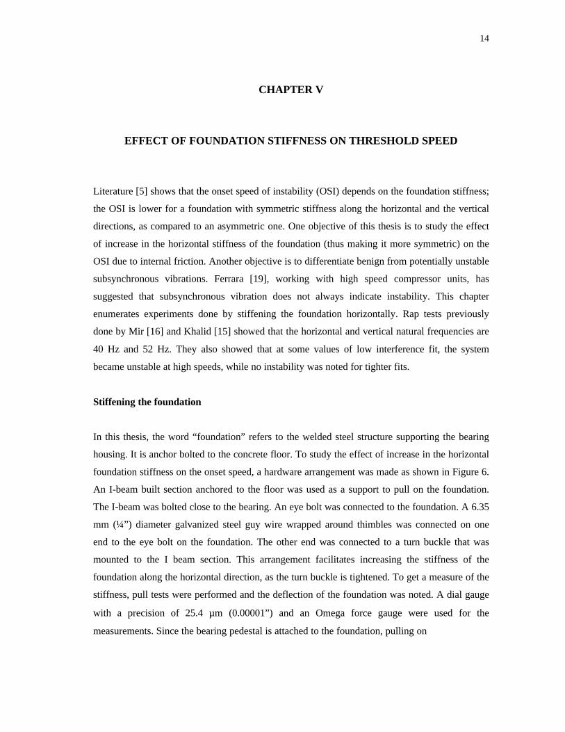
foundation stiffness on the onset speed, a hardware arrangement was made as shown in Figure 6.

An I-beam built section anchored to the floor was used as a support to pull on the foundation.

The I-beam was bolted close to the bearing. An eye bolt was connected to the foundation. A 6.35

mm (¼”) diameter galvanized steel guy wire wrapped around thimbles was connected on one

end to the eye bolt on the foundation. The other end was connected to a turn buckle that was

mounted to the I beam section. This arrangement facilitates increasing the stiffness of the

foundation along the horizontal direction, as the turn buckle is tightened. To get a measure of the

stiffness, pull tests were performed and the deflection of the foundation was noted. A dial gauge

with a precision of 25.4 µm (0.00001”) and an Omega force gauge were used for the

measurements. Since the bearing pedestal is attached to the foundation, pulling on

15

Figure 6: Arrangement to constrain the foundation

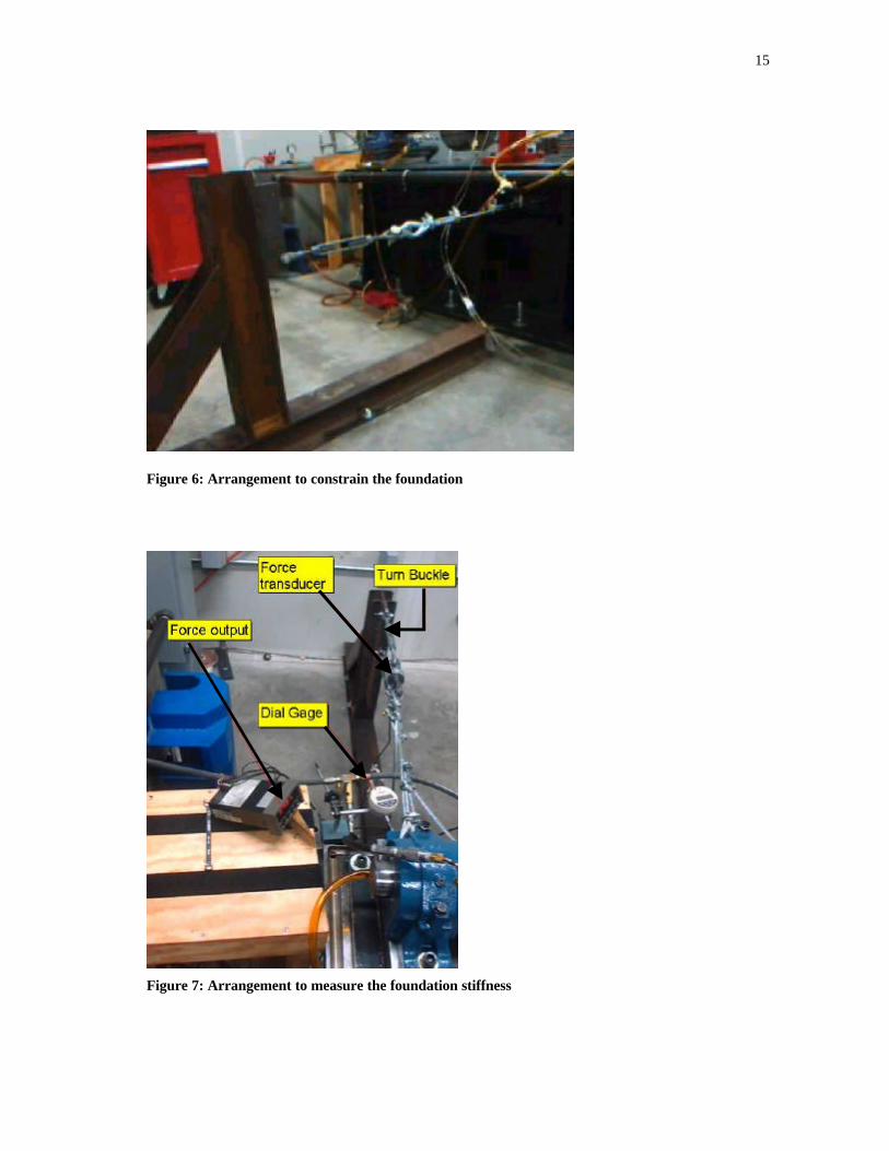
Figure 7: Arrangement to measure the foundation stiffness

16

the bearing pedestal would result in a deflection of the foundation. A thimble was secured to the

bearing housing, and the steel guy wire was routed through this thimble. This wire was

connected to the force gauge, as shown in Figure 7.

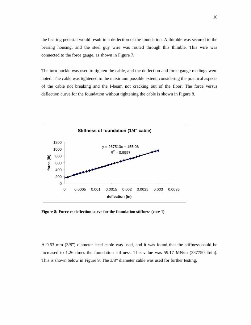
The turn buckle was used to tighten the cable, and the deflection and force gauge readings were

noted. The cable was tightened to the maximum possible extent, considering the practical aspects

of the cable not breaking and the I-beam not cracking out of the floor. The force versus

deflection curve for the foundation without tightening the cable is shown in Figure 8.

Stiffness of foundation (1/4" cable)

y = 267513x + 155.06

R2 = 0.9997

0

200

400

600

800

1000

1200

0 0.0005 0.001 0.0015 0.002 0.0025 0.003 0.0035

deflection (in)

forc

e (l

b)

Figure 8: Force vs deflection curve for the foundation stiffness (case 1)

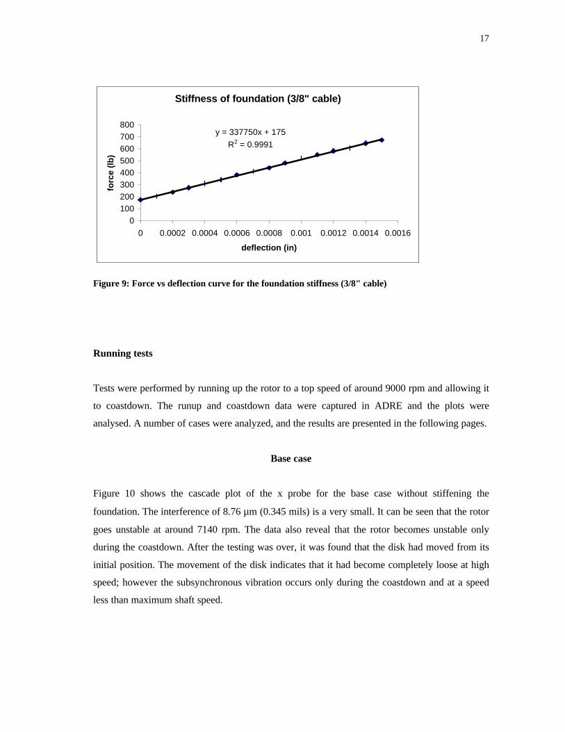
A 9.53 mm (3/8”) diameter steel cable was used, and it was found that the stiffness could be

increased to 1.26 times the foundation stiffness. This value was 59.17 MN/m (337750 lb/in).

This is shown below in Figure 9. The 3/8” diameter cable was used for further testing.

17

Stiffness of foundation (3/8" cable)

y = 337750x + 175

R2 = 0.9991

0100200300400500600700800

0 0.0002 0.0004 0.0006 0.0008 0.001 0.0012 0.0014 0.0016

deflection (in)

forc

e (l

b)

Figure 9: Force vs deflection curve for the foundation stiffness (3/8" cable)

Running tests

Tests were performed by running up the rotor to a top speed of around 9000 rpm and allowing it

to coastdown. The runup and coastdown data were captured in ADRE and the plots were

analysed. A number of cases were analyzed, and the results are presented in the following pages.

Base case

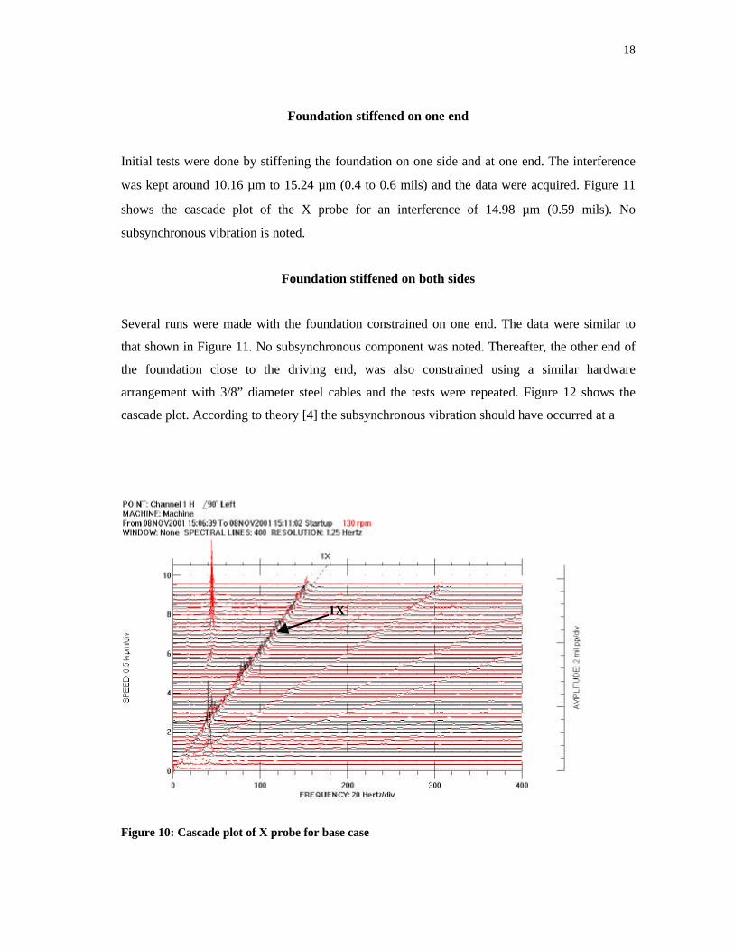
Figure 10 shows the cascade plot of the x probe for the base case without stiffening the

foundation. The interference of 8.76 µm (0.345 mils) is a very small. It can be seen that the rotor

goes unstable at around 7140 rpm. The data also reveal that the rotor becomes unstable only

during the coastdown. After the testing was over, it was found that the disk had moved from its

initial position. The movement of the disk indicates that it had become completely loose at high

speed; however the subsynchronous vibration occurs only during the coastdown and at a speed

less than maximum shaft speed.

18

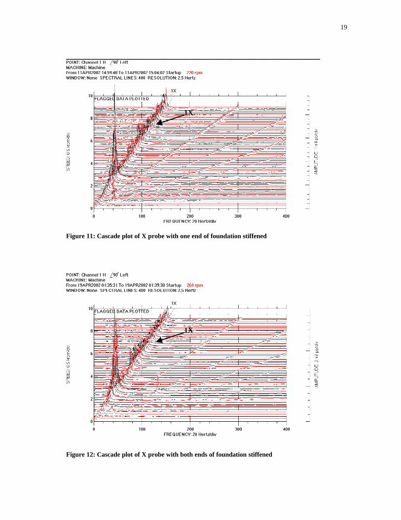
Foundation stiffened on one end

Initial tests were done by stiffening the foundation on one side and at one end. The interference

was kept around 10.16 µm to 15.24 µm (0.4 to 0.6 mils) and the data were acquired. Figure 11

shows the cascade plot of the X probe for an interference of 14.98 µm (0.59 mils). No

subsynchronous vibration is noted.

Foundation stiffened on both sides

Several runs were made with the foundation constrained on one end. The data were similar to

that shown in Figure 11. No subsynchronous component was noted. Thereafter, the other end of

the foundation close to the driving end, was also constrained using a similar hardware

arrangement with 3/8” diameter steel cables and the tests were repeated. Figure 12 shows the

cascade plot. According to theory [4] the subsynchronous vibration should have occurred at a

Figure 10: Cascade plot of X probe for base case

1X

19

Figure 11: Cascade plot of X probe with one end of foundation stiffened

Figure 12: Cascade plot of X probe with both ends of foundation stiffened

1X

1X

20

lower shaft speed (compared to the base case) when the foundation stiffness was increased and

made more symmetric, but in fact it disappeared.

Effect of balancing

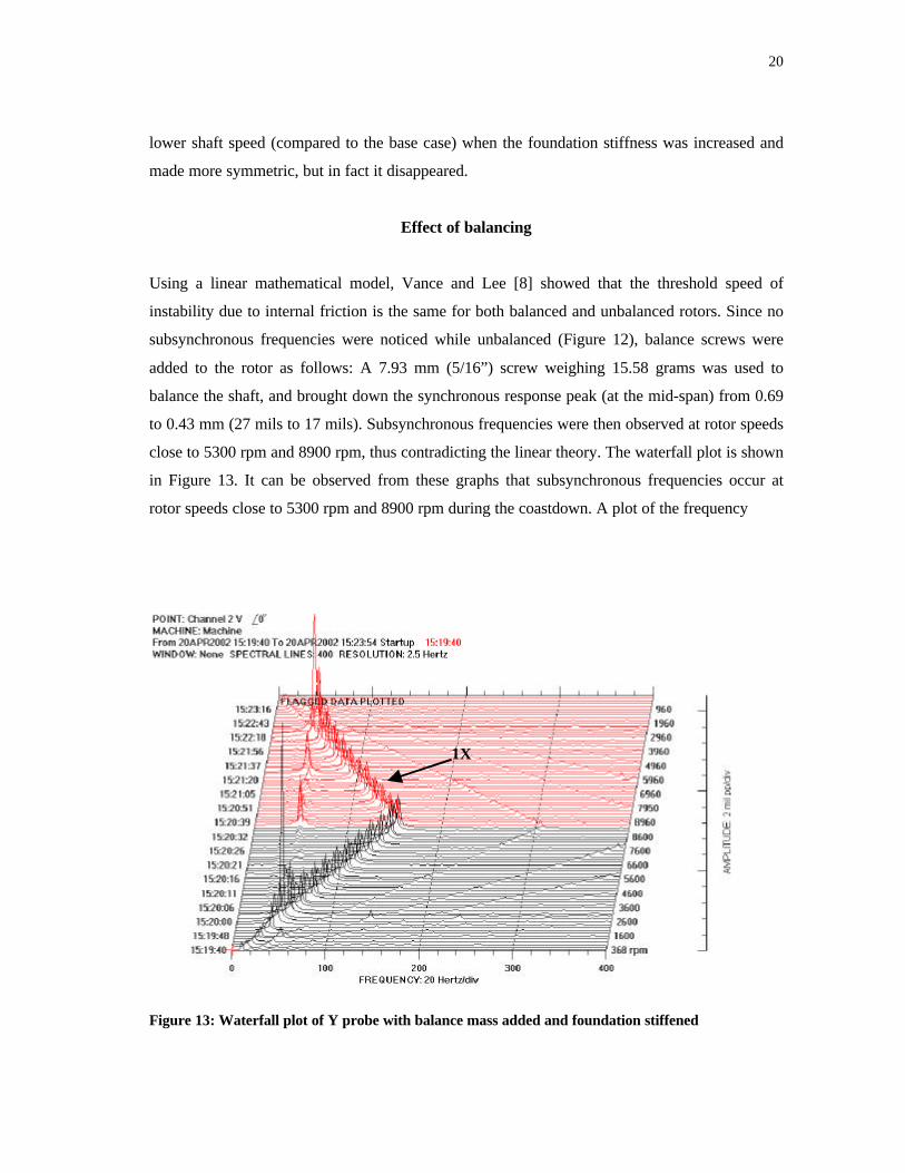
Using a linear mathematical model, Vance and Lee [8] showed that the threshold speed of

instability due to internal friction is the same for both balanced and unbalanced rotors. Since no

subsynchronous frequencies were noticed while unbalanced (Figure 12), balance screws were

added to the rotor as follows: A 7.93 mm (5/16”) screw weighing 15.58 grams was used to

balance the shaft, and brought down the synchronous response peak (at the mid-span) from 0.69

to 0.43 mm (27 mils to 17 mils). Subsynchronous frequencies were then observed at rotor speeds

close to 5300 rpm and 8900 rpm, thus contradicting the linear theory. The waterfall plot is shown

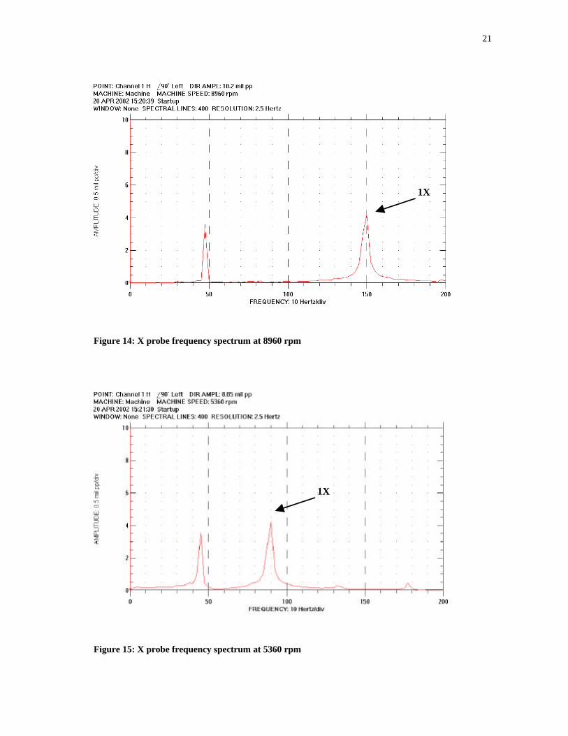
in Figure 13. It can be observed from these graphs that subsynchronous frequencies occur at

rotor speeds close to 5300 rpm and 8900 rpm during the coastdown. A plot of the frequency

Figure 13: Waterfall plot of Y probe with balance mass added and foundation stiffened

1X

21

Figure 14: X probe frequency spectrum at 8960 rpm

Figure 15: X probe frequency spectrum at 5360 rpm

1X

1X

22

spectrum at 8960 rpm and 5350 rpm is shown in Figures 14,15. The subsynchronous components

at 8960 and 5360 rpm appeared after the addition of the balance screw. Gunter [20] reported

similar experimental results where balancing made oil whirl more severe. These results

contradict the prediction of the linear model of Vance and Lee [8].

Addition of anti-seize compound

To avoid seizure of the mating parts due to interference fit in rotors, common industry practice is

to apply an anti-seize compound on the surfaces in contact. To simulate this condition and

investigate its effect on rotordynamic stability, anti-seize compound was applied on the sleeve so

that as the disk slides on the sleeve, the anti-seize compound action comes into play. The same

type of signatures were noted for the tests with and without the anti-seize: the anti-seize had no

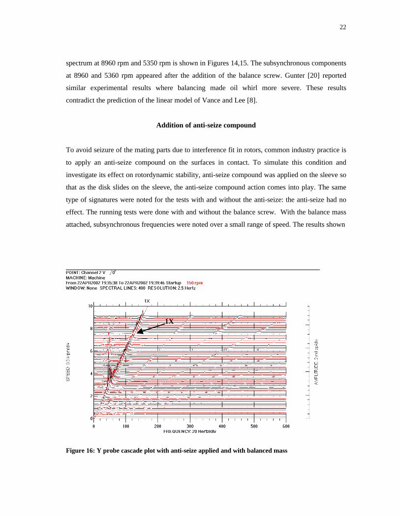
effect. The running tests were done with and without the balance screw. With the balance mass

attached, subsynchronous frequencies were noted over a small range of speed. The results shown

Figure 16: Y probe cascade plot with anti-seize applied and with balanced mass

1X

23

Figure 17: Y probe waterfall plot with anti-seize applied and with balanced mass

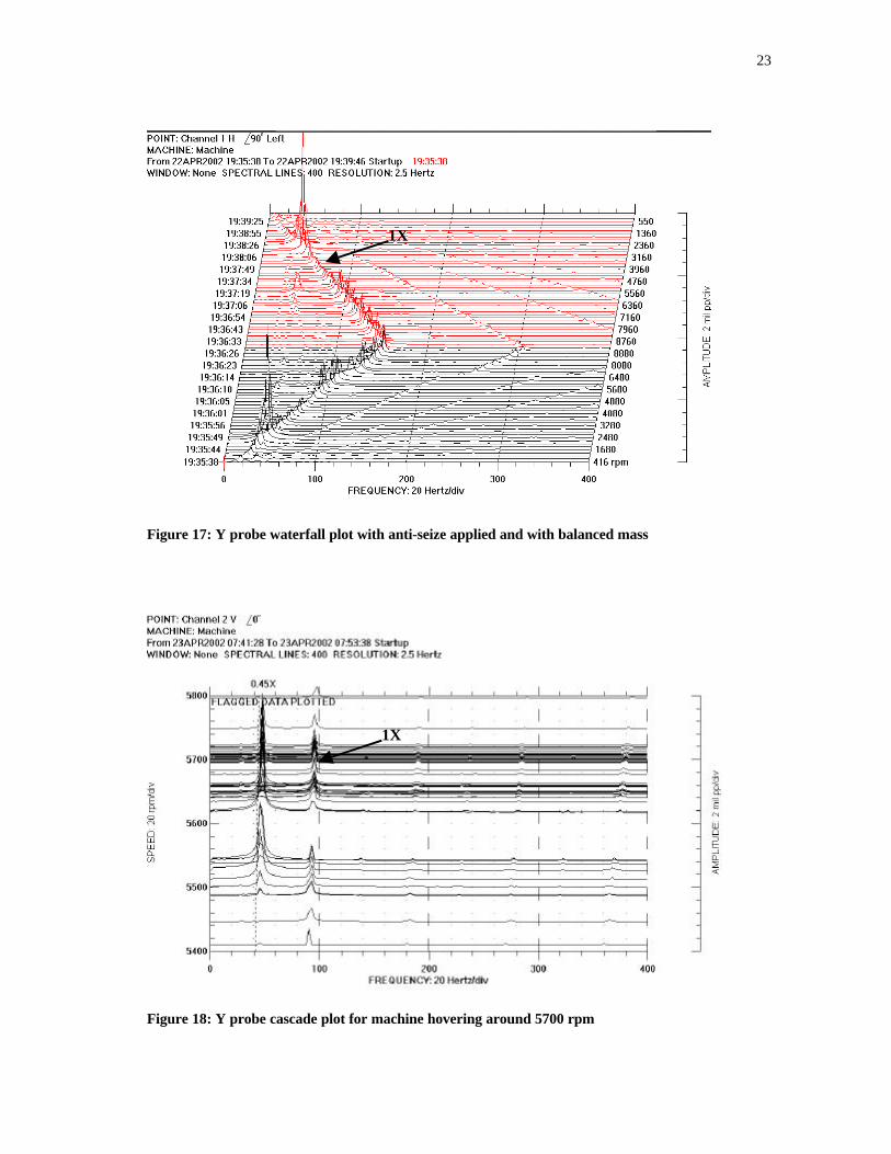
Figure 18: Y probe cascade plot for machine hovering around 5700 rpm

1X

1X

24

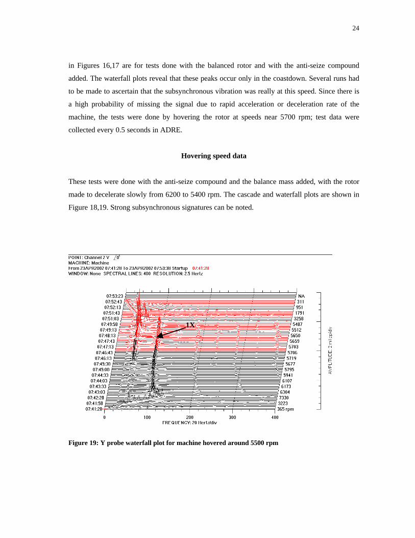
in Figures 16,17 are for tests done with the balanced rotor and with the anti-seize compound

added. The waterfall plots reveal that these peaks occur only in the coastdown. Several runs had

to be made to ascertain that the subsynchronous vibration was really at this speed. Since there is

a high probability of missing the signal due to rapid acceleration or deceleration rate of the

machine, the tests were done by hovering the rotor at speeds near 5700 rpm; test data were

collected every 0.5 seconds in ADRE.

Hovering speed data

These tests were done with the anti-seize compound and the balance mass added, with the rotor

made to decelerate slowly from 6200 to 5400 rpm. The cascade and waterfall plots are shown in

Figure 18,19. Strong subsynchronous signatures can be noted.

Figure 19: Y probe waterfall plot for machine hovered around 5500 rpm

1X

25

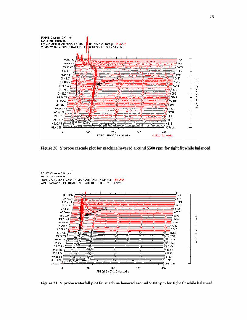
Figure 20: Y probe cascade plot for machine hovered around 5500 rpm for tight fit while balanced

Figure 21: Y probe waterfall plot for machine hovered around 5500 rpm for tight fit while balanced

1X

1X

26

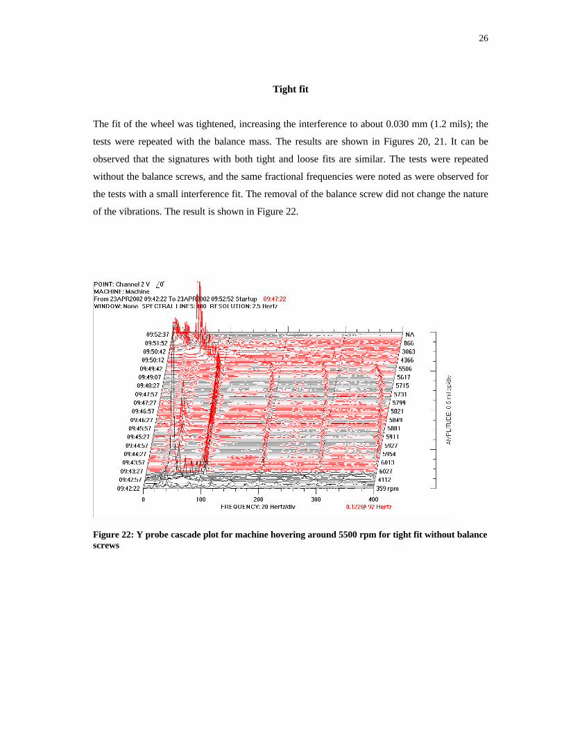
Tight fit

The fit of the wheel was tightened, increasing the interference to about 0.030 mm (1.2 mils); the

tests were repeated with the balance mass. The results are shown in Figures 20, 21. It can be

observed that the signatures with both tight and loose fits are similar. The tests were repeated

without the balance screws, and the same fractional frequencies were noted as were observed for

the tests with a small interference fit. The removal of the balance screw did not change the nature

of the vibrations. The result is shown in Figure 22.

Figure 22: Y probe cascade plot for machine hovering around 5500 rpm for tight fit without balancescrews

27

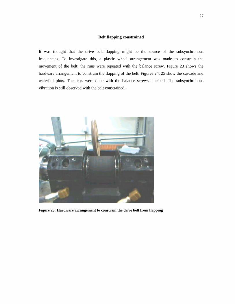
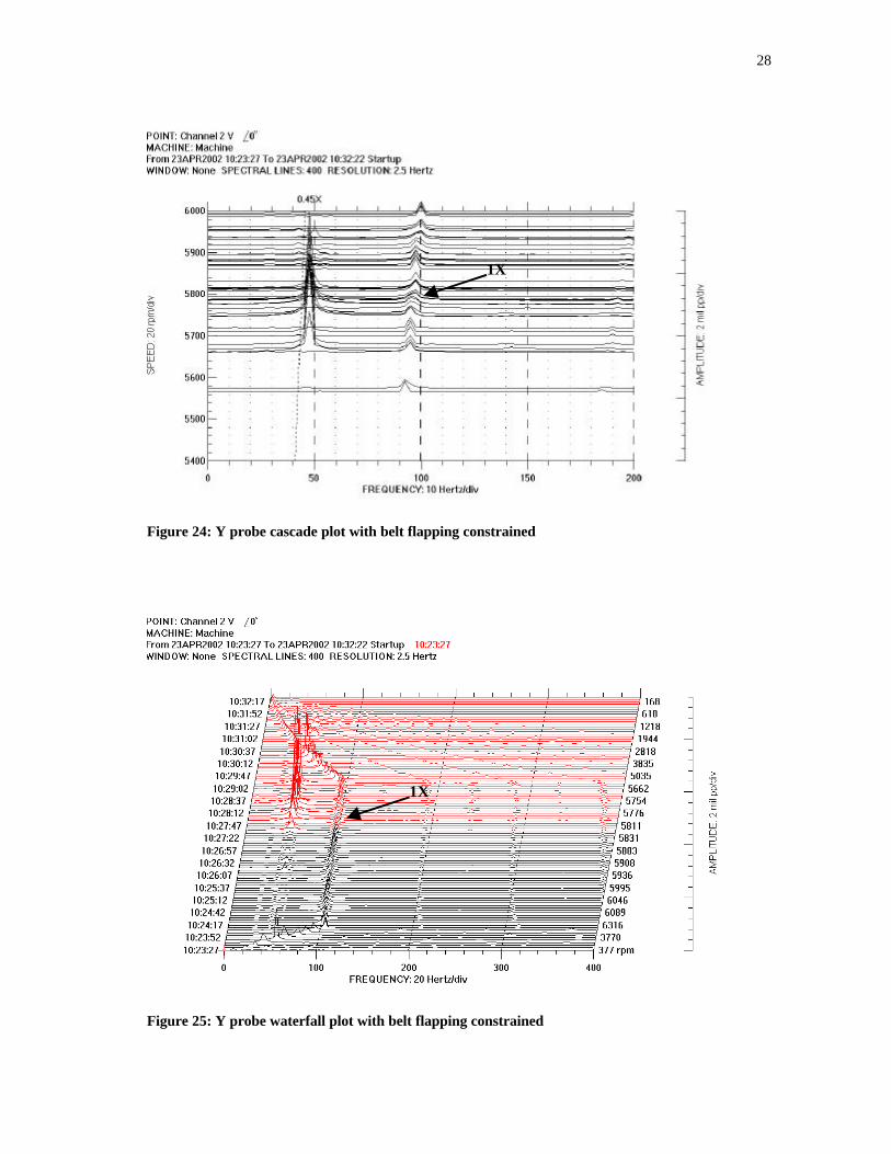
Belt flapping constrained

It was thought that the drive belt flapping might be the source of the subsynchronous

frequencies. To investigate this, a plastic wheel arrangement was made to constrain the

movement of the belt; the runs were repeated with the balance screw. Figure 23 shows the

hardware arrangement to constrain the flapping of the belt. Figures 24, 25 show the cascade and

waterfall plots. The tests were done with the balance screws attached. The subsynchronous

vibration is still observed with the belt constrained.

Figure 23: Hardware arrangement to constrain the drive belt from flapping

28

Figure 24: Y probe cascade plot with belt flapping constrained

Figure 25: Y probe waterfall plot with belt flapping constrained

1X

1X

29

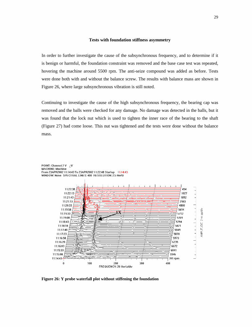
Tests with foundation stiffness asymmetry

In order to further investigate the cause of the subsynchronous frequency, and to determine if it

is benign or harmful, the foundation constraint was removed and the base case test was repeated,

hovering the machine around 5500 rpm. The anti-seize compound was added as before. Tests

were done both with and without the balance screw. The results with balance mass are shown in

Figure 26, where large subsynchronous vibration is still noted.

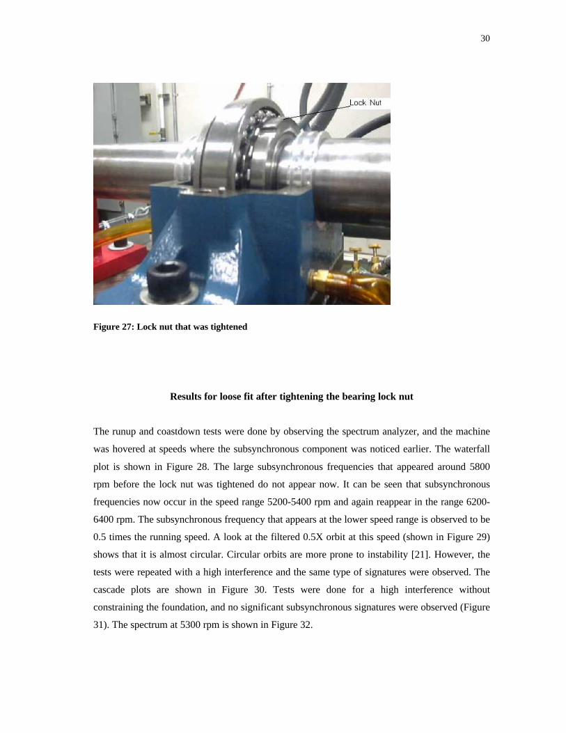
Continuing to investigate the cause of the high subsynchronous frequency, the bearing cap was

removed and the balls were checked for any damage. No damage was detected in the balls, but it

was found that the lock nut which is used to tighten the inner race of the bearing to the shaft

(Figure 27) had come loose. This nut was tightened and the tests were done without the balance

mass.

Figure 26: Y probe waterfall plot without stiffening the foundation

1X

30

Figure 27: Lock nut that was tightened

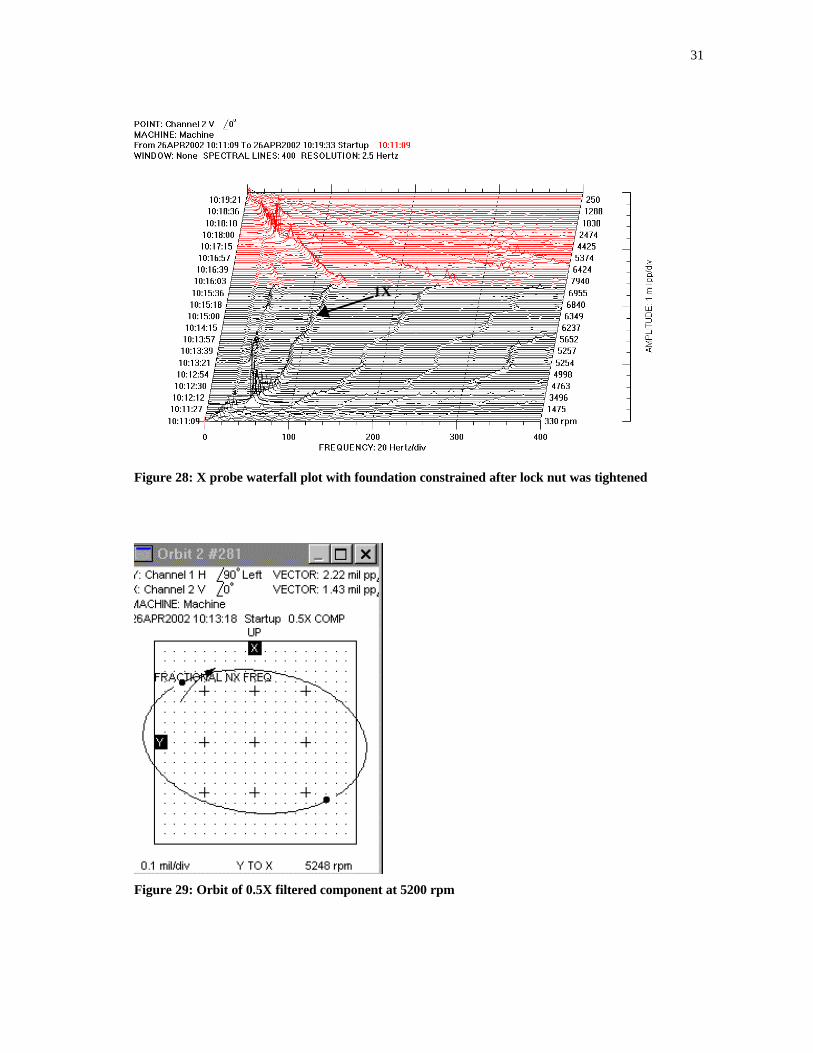
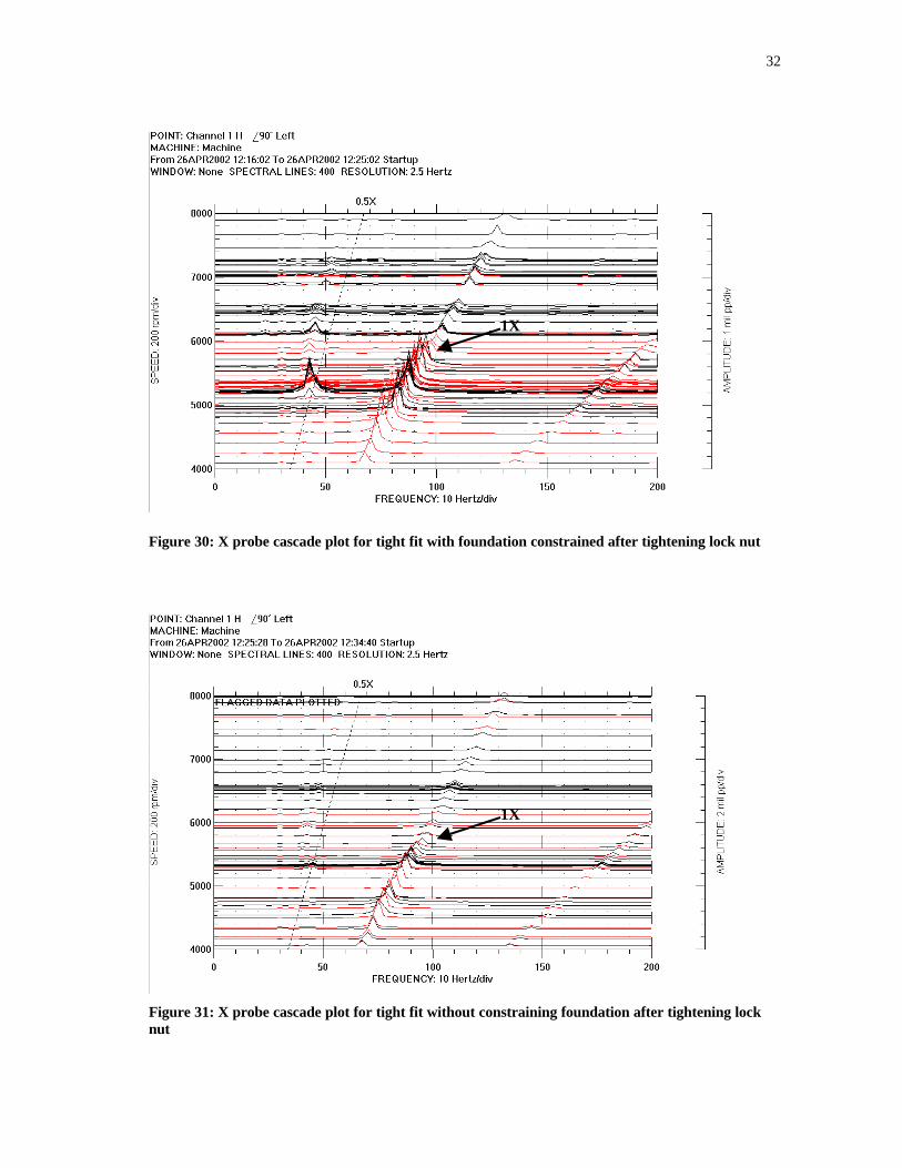
Results for loose fit after tightening the bearing lock nut

The runup and coastdown tests were done by observing the spectrum analyzer, and the machine

was hovered at speeds where the subsynchronous component was noticed earlier. The waterfall

plot is shown in Figure 28. The large subsynchronous frequencies that appeared around 5800

rpm before the lock nut was tightened do not appear now. It can be seen that subsynchronous

frequencies now occur in the speed range 5200-5400 rpm and again reappear in the range 6200-

6400 rpm. The subsynchronous frequency that appears at the lower speed range is observed to be

0.5 times the running speed. A look at the filtered 0.5X orbit at this speed (shown in Figure 29)

shows that it is almost circular. Circular orbits are more prone to instability [21]. However, the

tests were repeated with a high interference and the same type of signatures were observed. The

cascade plots are shown in Figure 30. Tests were done for a high interference without

constraining the foundation, and no significant subsynchronous signatures were observed (Figure

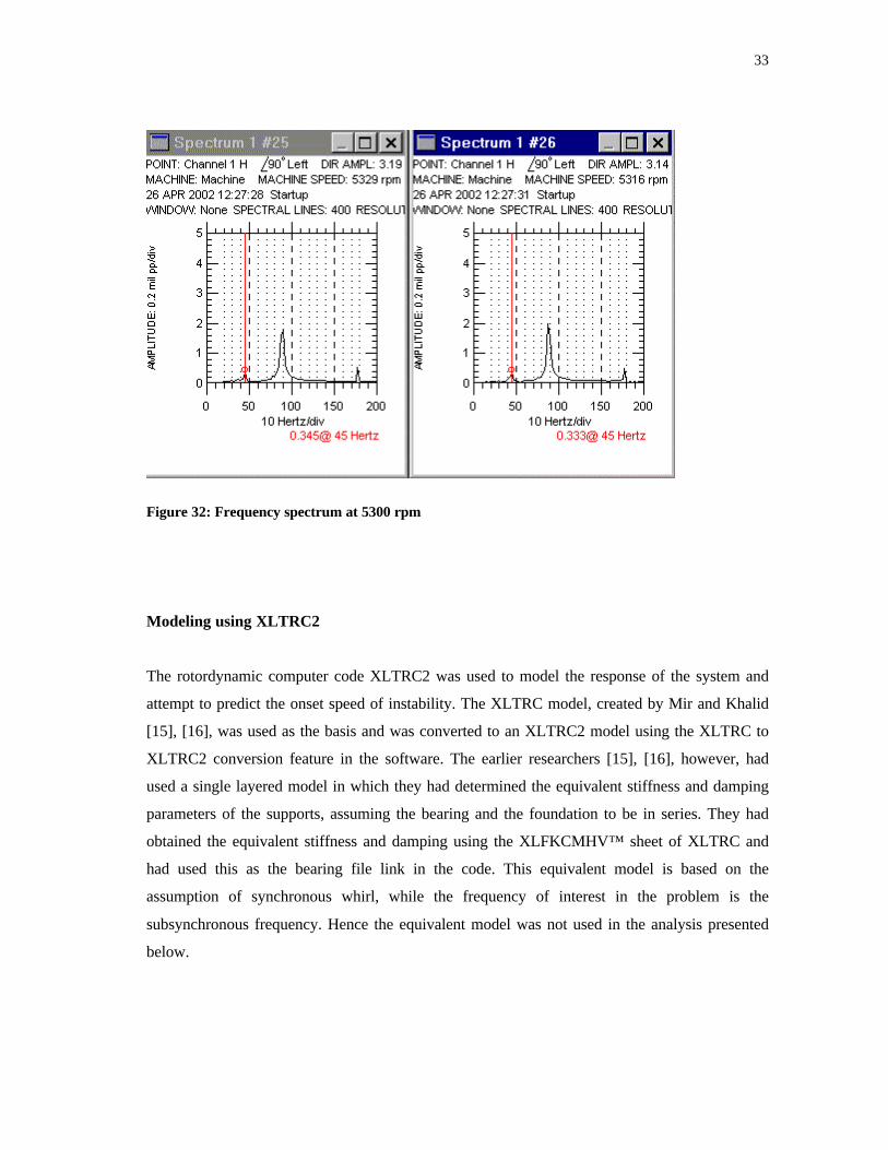
31). The spectrum at 5300 rpm is shown in Figure 32.

31

Figure 28: X probe waterfall plot with foundation constrained after lock nut was tightened

Figure 29: Orbit of 0.5X filtered component at 5200 rpm

1X

32

Figure 30: X probe cascade plot for tight fit with foundation constrained after tightening lock nut

Figure 31: X probe cascade plot for tight fit without constraining foundation after tightening locknut

1X

1X

33

Figure 32: Frequency spectrum at 5300 rpm

Modeling using XLTRC2

The rotordynamic computer code XLTRC2 was used to model the response of the system and

attempt to predict the onset speed of instability. The XLTRC model, created by Mir and Khalid

[15], [16], was used as the basis and was converted to an XLTRC2 model using the XLTRC to

XLTRC2 conversion feature in the software. The earlier researchers [15], [16], however, had

used a single layered model in which they had determined the equivalent stiffness and damping

parameters of the supports, assuming the bearing and the foundation to be in series. They had

obtained the equivalent stiffness and damping using the XLFKCMHV™ sheet of XLTRC and

had used this as the bearing file link in the code. This equivalent model is based on the

assumption of synchronous whirl, while the frequency of interest in the problem is the

subsynchronous frequency. Hence the equivalent model was not used in the analysis presented

below.

34

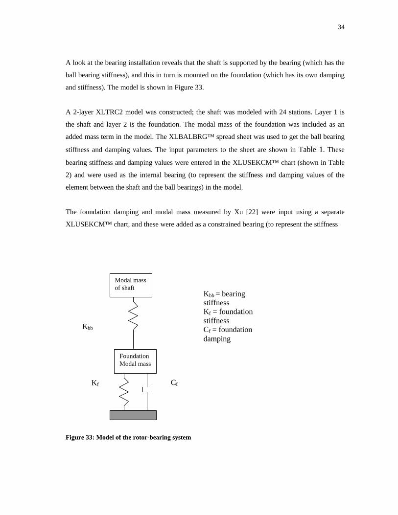
A look at the bearing installation reveals that the shaft is supported by the bearing (which has the

ball bearing stiffness), and this in turn is mounted on the foundation (which has its own damping

and stiffness). The model is shown in Figure 33.

A 2-layer XLTRC2 model was constructed; the shaft was modeled with 24 stations. Layer 1 is

the shaft and layer 2 is the foundation. The modal mass of the foundation was included as an

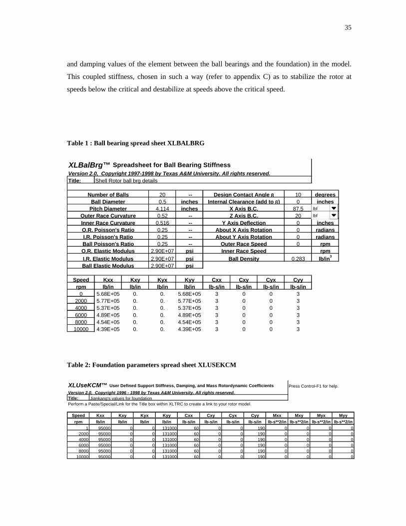
added mass term in the model. The XLBALBRG™ spread sheet was used to get the ball bearing

stiffness and damping values. The input parameters to the sheet are shown in Table 1. These

bearing stiffness and damping values were entered in the XLUSEKCM™ chart (shown in Table

2) and were used as the internal bearing (to represent the stiffness and damping values of the

element between the shaft and the ball bearings) in the model.

The foundation damping and modal mass measured by Xu [22] were input using a separate

XLUSEKCM™ chart, and these were added as a constrained bearing (to represent the stiffness

FoundationModal mass

Kbb = bearingstiffnessKf = foundationstiffnessCf = foundationdamping

Modal massof shaft

Kf Cf

Kbb

Figure 33: Model of the rotor-bearing system

35

and damping values of the element between the ball bearings and the foundation) in the model.

This coupled stiffness, chosen in such a way (refer to appendix C) as to stabilize the rotor at

speeds below the critical and destabilize at speeds above the critical speed.

Table 1 : Ball bearing spread sheet XLBALBRG

XLBalBrg™ Spreadsheet for Ball Bearing StiffnessVersion 2.0, Copyright 1997-1998 by Texas A&M University. All rights reserved.Title: Shell Rotor ball brg details

Number of Balls 20 -- Design Contact Angle ββ 10 degreesBall Diameter 0.5 inches Internal Clearance (add to ββ) 0 inches

Pitch Diameter 4.114 inches X Axis B.C. 87.5Outer Race Curvature 0.52 -- Z Axis B.C. 20Inner Race Curvature 0.516 -- Y Axis Deflection 0 inchesO.R. Poisson's Ratio 0.25 -- About X Axis Rotation 0 radiansI.R. Poisson's Ratio 0.25 -- About Y Axis Rotation 0 radiansBall Poisson's Ratio 0.25 -- Outer Race Speed 0 rpmO.R. Elastic Modulus 2.90E+07 psi Inner Race Speed rpmI.R. Elastic Modulus 2.90E+07 psi Ball Density 0.283 lb/in3

Ball Elastic Modulus 2.90E+07 psi

Speed Kxx Kxy Kyx Kyy Cxx Cxy Cyx Cyyrpm lb/in lb/in lb/in lb/in lb-s/in lb-s/in lb-s/in lb-s/in

0 5.68E+05 0. 0. 5.68E+05 3 0 0 32000 5.77E+05 0. 0. 5.77E+05 3 0 0 34000 5.37E+05 0. 0. 5.37E+05 3 0 0 36000 4.89E+05 0. 0. 4.89E+05 3 0 0 38000 4.54E+05 0. 0. 4.54E+05 3 0 0 310000 4.39E+05 0. 0. 4.39E+05 3 0 0 3

lbf

lbf

Table 2: Foundation parameters spread sheet XLUSEKCM

XLUseKCM™ User Defined Support Stiffness, Damping, and Mass Rotordynamic Coefficients Press Control-F1 for help.

Version 2.0, Copyright 1996 - 1998 by Texas A&M University. All rights reserved.Title: Jiankang's values for foundationPerform a Paste/Special/Link for the Title box within XLTRC to create a link to your rotor model.

Speed Kxx Kxy Kyx Kyy Cxx Cxy Cyx Cyy Mxx Mxy Myx Myyrpm lb/in lb/in lb/in lb/in lb-s/in lb-s/in lb-s/in lb-s/in lb-s**2/in lb-s**2/in lb-s**2/in lb-s**2/in

1 95000 0 0 131000 60 0 0 190 0 0 0 02000 95000 0 0 131000 60 0 0 190 0 0 0 04000 95000 0 0 131000 60 0 0 190 0 0 0 06000 95000 0 0 131000 60 0 0 190 0 0 0 08000 95000 0 0 131000 60 0 0 190 0 0 0 0

10000 95000 0 0 131000 60 0 0 190 0 0 0 0

36

Table 3: Cross coupled stiffness terms sheet XLFKCMHV

XLUseKCM™ User Defined Support Stiffness, Damping, and Mass Rotordynamic Coefficients

Version 2.0, Copyright 1996 - 1998 by Texas A&M University. All rights reserved.Title: Damping Kxy and Kyx Perform a Paste/Special/Link for the Title box within XLTRC to create a link to your rotor model.

Speed Kxx Kxy Kyx Kyy Cxx Cxyrpm lb/in lb/in lb/in lb/in lb-s/in lb-s/in

1 0. -1. 1. 0 0 0185 0. -116. 116. 0 0 0369 0. -232. 232. 0 0 0554 0. -348. 348. 0 0 0738 0. -464. 464. 0 0 0923 0. -580. 580. 0 0 0

1,108 0. -696. 696. 0 0 01,292 0. -812. 812. 0 0 01,477 0. -928. 928. 0 0 01,662 0. -1044. 1044. 0 0 01,846 0. -1160. 1160. 0 0 02,031 0. -1276. 1276. 0 0 02,215 0. -1392. 1392. 0 0 02,400 0. -1508. 1508. 0 0 02,585 0. -1624. 1624. 0 0 02,769 0. -1740. 1740. 0 0 02,954 0. -1856. 1856. 0 0 03,138 0. 1972. -1972. 0 0 03,323 0. 2088. -2088. 0 0 03,508 0. 2204. -2204. 0 0 03,692 0. 2320. -2320. 0 0 03,877 0. 2436. -2436. 0 0 0

The magnitude of the internal friction was adjusted until it closely predicted the threshold speed

of instability for the case without stiffening the foundation. This value turned out to be 6 lb-s/in.

The sheet used for the cross-coupled stiffness terms is shown in Table 3.

In summary, the two-layered model was constructed with the shaft as the first layer and the

foundation as the second layer. The foundation mass was added as an inertia term to the second

layer, and this second layer was made non-rotating (the rotation value in the model sheet of

XLTRC2 was 0). The geo plot of the model is shown in Figure 34.

37

Shaft330

Shaft328

Shaft227

Shaft225

Shaft124

2016

12

84Shaft1

1

-16

-12

-8

-4

0

4

8

12

16

0 8 16 24 32 40 48

Axial Location, inches

Sh

aft

Rad

ius,

in

ches

Shell Rotor test rig

Modeling the Interference fit

Figure 34: Geo plot of the rotor

The foundation modal mass and the stiffness were varied to match the horizontal and the vertical

direction Bode plot results of the model without the cross-coupled stiffness terms. The matched

results are shown in Figure 35, 36.

The eigenvalue analysis of XLTRC2 predicts that the rotor goes unstable at 7385 rpm (Table 4).

The running tests reveal instability at speed close to 7100 rpm. The stiffness along the horizontal

axis was increased (the value of Kxx in the foundation parameters was increased) and, the model

then predicts that the rotor will become unstable at 5169 rpm. This instability is shown in Table

5, and was observed in the experiments done both with the foundation stiffened horizontally and

with tight and loose fits.

38

Horizontal Bode plot

0

2

4

6

8

10

12

-1000 1000 3000 5000 7000

speed(rpm)

amp

litu

de(

p-p

, mils

)

running test data

XLTRC2 result

Figure 35: Horizontal Bode plot matched for base case

Vertical Bode plot

0123456789

10

0 2000 4000 6000 8000

speed(rpm)

amp

litu

de(

p-p

, mils

)

running test data

XLTRC2 result

Figure 36: Vertical Bode plot matched for base case

39

Table 4: Damped roots showing onset speed of instability at 7385 rpm

Speed zeta1 cpm1 zeta2 cpm2 zeta35169. 0.000 9.7 0.035 2723.1 0.0635354. 0.000 9.7 0.033 2732.2 0.0665538. 0.000 9.7 0.030 2740.9 0.0685723. 0.000 9.7 0.027 2748.2 0.0725908. 0.000 9.7 0.023 2754.1 0.0756092. 0.000 9.7 0.020 2758.7 0.0796277. 0.000 9.7 0.016 2762.4 0.0826462. 0.000 9.7 0.013 2765.6 0.0856646. 0.000 9.7 0.010 2768.3 0.0886831. 0.000 9.7 0.007 2770.7 0.0917015. 0.000 9.7 0.004 2772.8 0.0947200. 0.000 9.7 0.001 2774.8 0.097

7385. 0.000 9.7 -0.002 2776.7 0.1007569. 0.000 9.7 -0.005 2778.5 0.1027754. 0.000 9.7 -0.008 2780.2 0.1057938. 0.000 9.7 -0.010 2781.9 0.1088123. 0.000 9.7 -0.013 2783.5 0.1108308. 0.000 9.7 -0.016 2785.2 0.113

Table 5: Damped roots showing instability at 5169 rpm with horizontal foundation stiffness

increased

Speed zeta1 cpm1 zeta2 cpm2 zeta33323. 0.000 9.7 0.016 2835.7 0.0643508. 0.000 9.7 0.014 2837.6 0.0653692. 0.000 9.7 0.013 2839.5 0.0673877. 0.000 9.7 0.011 2841.3 0.0684062. 0.000 9.7 0.009 2843.0 0.0704246. 0.000 9.7 0.008 2844.6 0.0724431. 0.000 9.7 0.006 2846.2 0.0744615. 0.000 9.7 0.004 2847.6 0.0764800. 0.000 9.7 0.002 2848.9 0.0784985. 0.000 9.7 0.000 2850.2 0.080

5169. 0.000 9.7 -0.002 2851.4 0.0825354. 0.000 9.7 -0.005 2852.5 0.0845538. 0.000 9.7 -0.007 2853.6 0.0865723. 0.000 9.7 -0.009 2854.6 0.0885908. 0.000 9.7 -0.011 2855.6 0.0906092. 0.000 9.7 -0.013 2856.6 0.092

40

Discussion of results

An attempt was first made to understand the subsynchronous whirl of the base case as the

destabilizing effect of internal friction. The stiffness of the foundation was increased along the

horizontal direction to make it more symmetrically stiff along the x and the y directions. The

data then shows no instability without a balance mass. This contradicts the theory [5] that

predicts a stabilizing effect of support stiffness asymmetry. However, the addition of a balance

screw produced large subsynchronous signatures with the frequency slightly higher than 0.45

times the running speed. This contradicts the theory [8] that predicts no effect of unbalance.

Most of the subsynchronous peaks occurred over a very small range of the running speed.

Hence, the runup and coastdown data are not an ideal way to capture these subsynchronous

peaks. Tests done by hovering the machine around the speed of 5500 rpm revealed more useful

results.

The tests show that subsynchronous frequencies occurred in the range of 5500-5700 rpm

irrespective of the tightness of the fit (between the sleeve and the disk) and the stiffness of the

foundation. The large subsynchronous amplitude appeared only after balancing the rotor. The

drive belt was constrained, thus eliminating its possible effect on the vibration signature. After

locating a loose lock nut in the bearing as a cause of the high subsynchronous vibrations, the

tests were repeated. The data are presented in Figures 28 through 32. The largest amplitude

subsynchronous vibration peaks that appeared in Figures 13,18,19,20,21 disappear after the

bearing lock nut is tightened. The subsynchronous frequencies that remain are also seen to be

different. Lin [23] reports subsynchronous vibrations induced by radial clearances in ball bearing

supports. However subsynchronous vibration due to a loose ball bearing is from an externally

applied forcing function on the system and does not drive the system unstable (the orbit is

bounded). Internal friction produces a follower force that supplies energy to the system, and the

orbit grows exponentially before catastrophic failures could occur [24].

The “Fundamental Train Frequency” [24] created due to the rotation of the ball bearing cage is

given by

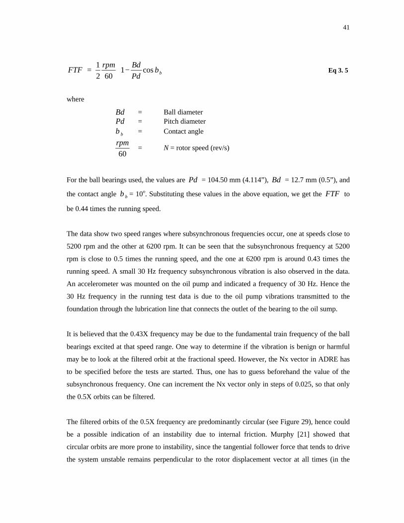
41

11 cos

2 60 b

rpm BdFTF

Pdβ = −

Eq 3. 5

where

Bd = Ball diameter Pd = Pitch diameter

bβ = Contact angle

60

rpm = N = rotor speed (rev/s)

For the ball bearings used, the values are Pd = 104.50 mm (4.114”), Bd = 12.7 mm (0.5”), and

the contact angle bβ = 10o. Substituting these values in the above equation, we get the FTF to

be 0.44 times the running speed.

The data show two speed ranges where subsynchronous frequencies occur, one at speeds close to

5200 rpm and the other at 6200 rpm. It can be seen that the subsynchronous frequency at 5200

rpm is close to 0.5 times the running speed, and the one at 6200 rpm is around 0.43 times the

running speed. A small 30 Hz frequency subsynchronous vibration is also observed in the data.

An accelerometer was mounted on the oil pump and indicated a frequency of 30 Hz. Hence the

30 Hz frequency in the running test data is due to the oil pump vibrations transmitted to the

foundation through the lubrication line that connects the outlet of the bearing to the oil sump.

It is believed that the 0.43X frequency may be due to the fundamental train frequency of the ball

bearings excited at that speed range. One way to determine if the vibration is benign or harmful

may be to look at the filtered orbit at the fractional speed. However, the Nx vector in ADRE has

to be specified before the tests are started. Thus, one has to guess beforehand the value of the

subsynchronous frequency. One can increment the Nx vector only in steps of 0.025, so that only

the 0.5X orbits can be filtered.

The filtered orbits of the 0.5X frequency are predominantly circular (see Figure 29), hence could

be a possible indication of an instability due to internal friction. Murphy [21] showed that

circular orbits are more prone to instability, since the tangential follower force that tends to drive

the system unstable remains perpendicular to the rotor displacement vector at all times (in the

42

same direction of the orbit velocity). However, the test data revealed subsynchronous

frequencies even with a tight fit (no internal friction). The data collected for the tight fit without

constraining the foundation (more asymmetry) reveal no large subsynchronous amplitudes, and

the 0.5X filtered orbits are elliptical.

These experiments suggest that subsynchronous vibration in rotating machinery can have

numerous sources or causes. Also the subsynchronous whirl due to internal friction is not a

highly repeatable phenomenon. The tests show subsynchronous frequencies only during the

coastdown, possibly due to the wheel becoming loose. The subsynchronous vibration depends on

the state of rotor balance. Subsynchronous vibrations can be produced by ball bearing dynamics,

a loose ball bearing or excitation from a nearby machine; therefore subsynchronous signatures

may not necessarily indicate instability.

43

CHAPTER VI

QUANTIFYING INTERNAL FRICTION

One of the problems associated with internal friction is the lack of numbers to characterize it.

Experiments at the laboratory have shown that the subsynchronous component due to internal

friction is not repeatable, and does not appear in all tests.

Mir [16] and Khalid [15] had done experiments with the taper-sleeve arrangement, but were

unable to produce enough friction to consistently drive the system unstable. Further, the

threshold speed was close to the maximum operating speed of the machine, making it difficult to

perform satisfactory tests. Bently and Muszynska [11] give a method of increasing the internal

friction by adding damping material in the form of a tape on the shaft. A self bonding (no glue)

tape was wrapped on both sides of the disk on our shaft in order to increase the internal friction.

By doing so, the threshold speed of instability was brought down to an analyzable speed. Runup

and coastdown tests were conducted on the rotor. This chapter summarizes the results both with

and without the self-bonding tape and both with and without the disk on the shaft.

Running tests

Runup and coastdown tests were done on the system for both high and low interference fits with

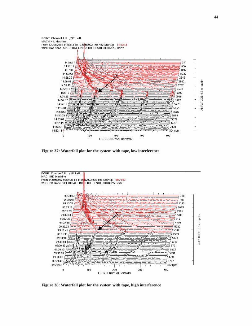
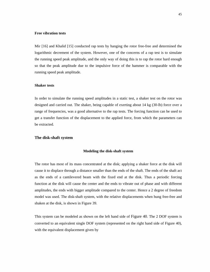
the tape and the results are shown in Figure 37 and 38. It can be seen that the onset speed of

instability is around 5500 rpm, much lower than for the tests done without the tape.

The same types of signatures were noted for both tight and loose fits of the disk. Hence it can be

argued that the subsynchronous frequency is due to the addition of the tape on the shaft. To

confirm this conclusion, the next step was to study the characteristics of the internal friction

induced by the tape. For this study the shaft was hung free-free and non-rotating tests were

conducted to determine the amount of internal damping.

44

Figure 37: Waterfall plot for the system with tape, low interference

Figure 38: Waterfall plot for the system with tape, high interference

1X

1X

45

Free vibration tests

Mir [16] and Khalid [15] conducted rap tests by hanging the rotor free-free and determined the

logarithmic decrement of the system. However, one of the concerns of a rap test is to simulate

the running speed peak amplitude, and the only way of doing this is to rap the rotor hard enough

so that the peak amplitude due to the impulsive force of the hammer is comparable with the

running speed peak amplitude.

Shaker tests

In order to simulate the running speed amplitudes in a static test, a shaker test on the rotor was

designed and carried out. The shaker, being capable of exerting about 14 kg (30-lb) force over a

range of frequencies, was a good alternative to the rap tests. The forcing function can be used to

get a transfer function of the displacement to the applied force, from which the parameters can

be extracted.

The disk-shaft system

Modeling the disk-shaft system

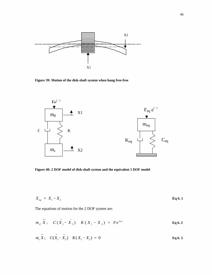
The rotor has most of its mass concentrated at the disk; applying a shaker force at the disk will

cause it to displace through a distance smaller than the ends of the shaft. The ends of the shaft act

as the ends of a cantilevered beam with the fixed end at the disk. Thus a periodic forcing

function at the disk will cause the center and the ends to vibrate out of phase and with different

amplitudes, the ends with bigger amplitude compared to the center. Hence a 2 degree of freedom

model was used. The disk-shaft system, with the relative displacements when hung free-free and

shaken at the disk, is shown in Figure 39.

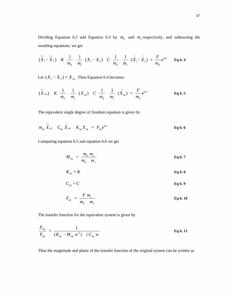
This system can be modeled as shown on the left hand side of Figure 40. The 2 DOF system is

converted to an equivalent single DOF system (represented on the right hand side of Figure 40),

with the equivalent displacement given by

46

X1

X2

Figure 39: Motion of the disk-shaft system when hung free-free

md

ms

Fei t

X1

X2

C K

meq

Feq ei t

Keq Ceq

Figure 40: 2 DOF model of disk-shaft system and the equivalent 1 DOF model

1 2eqX X X= − Eq 6. 1

The equations of motion for the 2 DOF system are:

1 1 2 1 2( ) ( ) i tdm X C X X K X X F e ω

• • • •

+ − + − = Eq 6. 2

2 1 2 1 2( ) ( ) 0sm X C X X K X X•• • •

+ − + − = Eq 6. 3

47

Dividing Equation 6.2 and Equation 6.3 by dm and sm respectively, and subtracting the

resulting equations, we get

1 2 1 2 1 2

1 1 1 1( ) ( ) ( ) i t

d s d s d

FX X K X X C X X e

m m m m mω

•• •• • • − + + − + + − =

Eq 6. 4

Let eqXXX =− )( 21 . Then Equation 6.4 becomes

1 1 1 1( ) ( ) ( ) i t

eq eq eqd s d s d

FX K X C X e

m m m m mω

•• • + + + + =

Eq 6. 5

The equivalent single degree of freedom equation is given by

i teq eqeq eq eq eq eqm X C X K X F e ω

•• •

+ + = Eq 6. 6

Comparing equation 6.5 and equation 6.6 we get

d seq

d s

m mM

m m=

+Eq 6. 7

KKeq = Eq 6. 8

CCeq = Eq 6. 9

seq

d s

F mF

m m=

+Eq 6. 10

The transfer function for the equivalent system is given by

2

1

( )eq

eq eq eq eq

X

F K M i Cω ω=

− +Eq 6. 11

Thus the magnitude and phase of the transfer function of the original system can be written as

48

[ ]

1 2

222

s

d s

s d

s d

m

m mX X

F m mK C

m mω ω

+−=

− + +

Eq 6. 12

1

2

tans d

s d

Cm m

Km m

ωφ

ω

−

= − +

Eq 6. 13

Determination of the disk ( dm ) and the shaft ( sm ) masses

The disk, being a heavy mass concentrated at the center, moves a smaller distance due to the

force compared to the ends of the shaft. Since the disk as a whole and a part of the shaft mass

participate in the motion, the mass of the disk dm that participates in the motion can be estimated

to be 110% of the disk mass.

1.1 45.45 50dm∴ = × = kg (110 lb)

The shaft is a cantilevered beam, with the ends tending to move in a direction opposite to the

applied force. For a cantilevered beam, the equivalent modal mass is 33/140 times the shaft mass

[17]. In this case, the shaft hangs on either side of the disk. Hence the mass of the shaft to be

considered will be twice the value of the shaft mass on one side multiplied by the fraction.

3317.05 2 8.04

140sm∴ = × × = kg (18 lb)

Determination of modal mass

The equivalent modal mass from equation 6.7 is 7.03 kg (15.47 lb).

The modal mass was also determined from the XLTRC2 model. The normalized zero speed

mode shape was determined and from the mass of each element, the modal mass was determined

from the equation

49

Free-Free Mode Shape PlotShell Rotor test rig

Modeling the Interference fit

f=7906.5 cpmN=1 rpm

forwardbackward

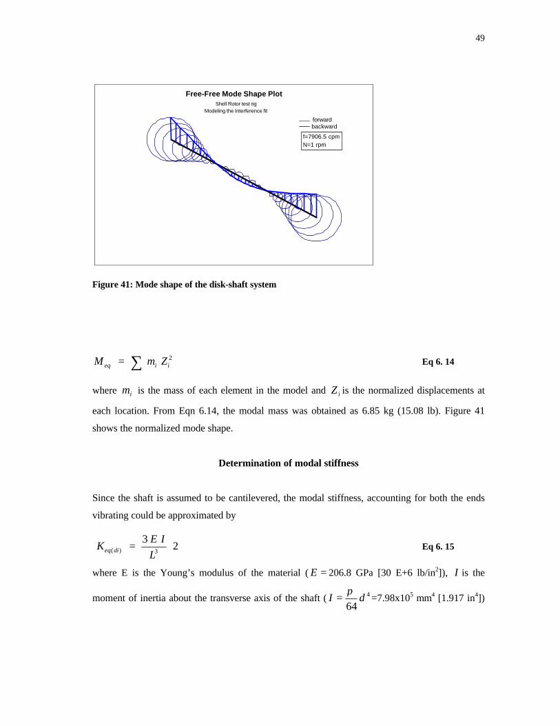
Figure 41: Mode shape of the disk-shaft system

2eq i iM m Z= ∑ Eq 6. 14

where im is the mass of each element in the model and iZ is the normalized displacements at

each location. From Eqn 6.14, the modal mass was obtained as 6.85 kg (15.08 lb). Figure 41

shows the normalized mode shape.

Determination of modal stiffness

Since the shaft is assumed to be cantilevered, the modal stiffness, accounting for both the ends

vibrating could be approximated by

( ) 3

32eq di

E IK

L= ⋅ Eq 6. 15

where E is the Young’s modulus of the material ( =E 206.8 GPa [30 E+6 lb/in2]), I is the

moment of inertia about the transverse axis of the shaft ( 4

64dI

π= =7.98x105 mm4 [1.917 in4])

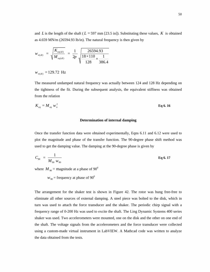
50

and L is the length of the shaft ( =L 597 mm [23.5 in]). Substituting these values, K is obtained

as 4.659 MN/m (26594.93 lb/in). The natural frequency is then given by

( )( )

( )

1 26594.9318 110 12

128 386.4

eq din di

eq di

K

Mω

π= =

××

72.129)( =dinω Hz

The measured undamped natural frequency was actually between 124 and 128 Hz depending on

the tightness of the fit. During the subsequent analysis, the equivalent stiffness was obtained

from the relation

2eq eq nK M ω= Eq 6. 16

Determination of internal damping

Once the transfer function data were obtained experimentally, Eqns 6.11 and 6.12 were used to

plot the magnitude and phase of the transfer function. The 90-degree phase shift method was

used to get the damping value. The damping at the 90-degree phase is given by

9090 90

1C

M ω= Eq 6. 17

where 90M = magnitude at a phase of 900

90ω = frequency at phase of 900

The arrangement for the shaker test is shown in Figure 42. The rotor was hung free-free to

eliminate all other sources of external damping. A steel piece was bolted to the disk, which in

turn was used to attach the force transducer and the shaker. The periodic chirp signal with a

frequency range of 0-200 Hz was used to excite the shaft. The Ling Dynamic Systems 400 series

shaker was used. Two accelerometers were mounted, one on the disk and the other on one end of

the shaft. The voltage signals from the accelerometers and the force transducer were collected

using a custom-made virtual instrument in LabVIEW. A Mathcad code was written to analyze

the data obtained from the tests.

51

Figure 42: Set-up arrangement

Analysis technique

The voltage data from the accelerometers and the force transducer were acquired using

LabVIEW. The frequency range and the resolution of the spectrum plots depend on the sampling

rate and the number of points acquired. The frequency span used in the shaker was 200 Hz,

starting from 0 Hz. To get a resolution of 0.5 Hz on the free spectrum, the number of points and

the sampling rate calculated were as follows:

The frequency resolution is related to the sampling rate ( sF ) and the number of samples ( N ) by

N

Ff s=∆ Eq 6. 18

Alternatively, f∆ can be expressed as

1f

N t∆ =

∆Eq 6. 19

where t∆ is the sampling period.

52

The shaker takes about two seconds (determined by the spectrum analyzer, which supplies the

frequencies to the shaker) to scan all frequencies from 0 to 200 Hz. If we acquire, say, 4096

samples, then

4096

2=∆t s Eq 6. 20(a)

From Eqn 6.18 we have

40965.0 sF

= Eq 6.20(b)

Hence the sampling rate was fixed at 2048 samples/s and 4096 points were gathered.

The following algorithm was used in Mathcad to analyze the data:

1. Acquire the time domain data points from the 2 accelerometers (manufactured by PCB) and

the force transducer (manufactured by PCB) with LabVIEW. (Units = V)

2. Convert the data to the required Engineering units using the sensitivities of the accelerometer

and the force transducer. The acceleration is now expressed in in/s2 and force in lb.

3. Convert the time domain data to the frequency domain using the FFT function in Mathcad.

4. Get the transfer function a2)/F-(a1 and convert that to X2)/F-(X1 by dividing it by the

square of the frequency at each frequency. (Units = in/lb)

5. Plot the magnitude and the phase of the transfer function and determine the damping from

equation 6.17 by interpolating the magnitude for the 90-degree phase.

In addition to the above-calculated values, the curve-fitting algorithm in Mathcad was also used

to get a set of values for the equivalent mass, stiffness and the internal damping. Thus 2 curves

were generated using equations 6.12 and 6.13: one set with the calculated values of the modal

parameters and the other with the values from the Mathcad curve-fit algorithm. These were

compared with the experimental curve.

Results for the disk-shaft system without tape

The tests were done for both low and high interference fits. It was found that the damping for the

low interference fit was higher than for the high interference. This is due to the fact that when

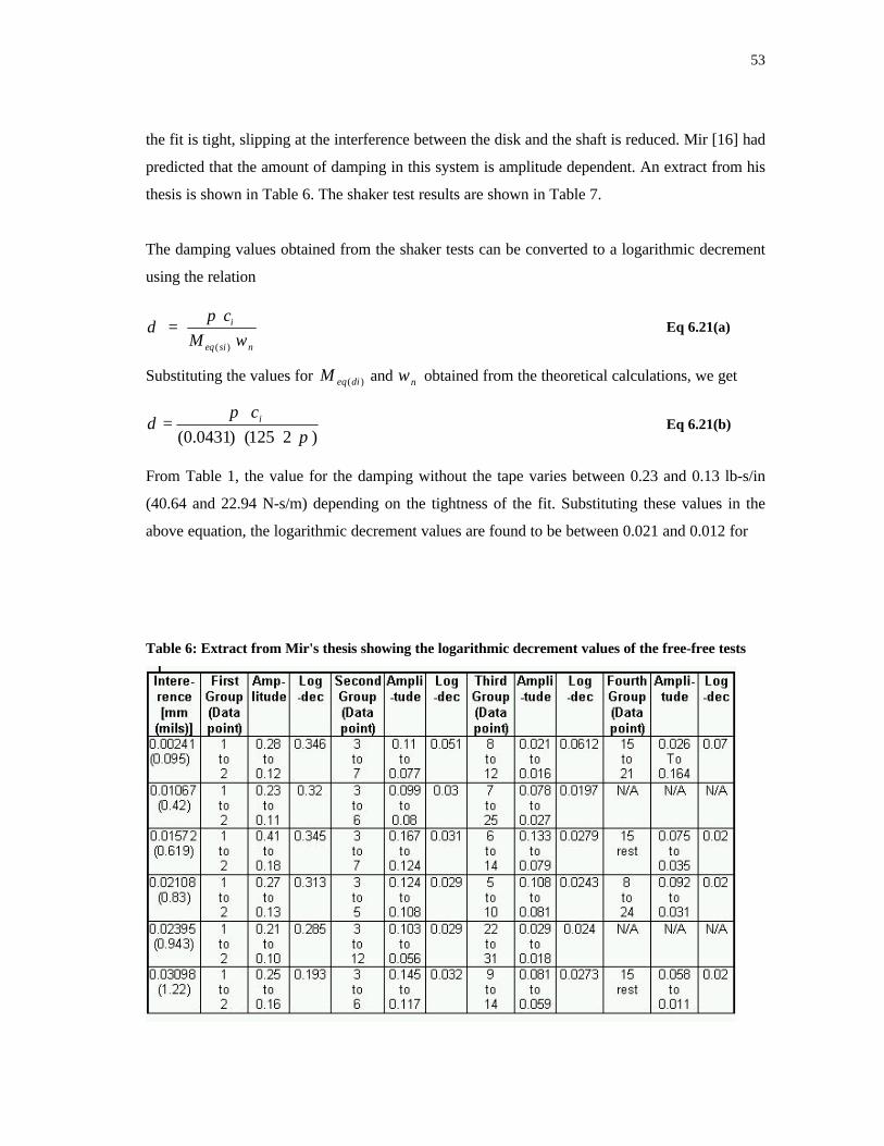
53

the fit is tight, slipping at the interference between the disk and the shaft is reduced. Mir [16] had

predicted that the amount of damping in this system is amplitude dependent. An extract from his

thesis is shown in Table 6. The shaker test results are shown in Table 7.

The damping values obtained from the shaker tests can be converted to a logarithmic decrement

using the relation

( )

i

eq si n

c

M

πδ

ω= Eq 6.21(a)

Substituting the values for )(dieqM and nω obtained from the theoretical calculations, we get

)2125()0431.0( ππ

δ⋅⋅⋅

⋅= ic

Eq 6.21(b)

From Table 1, the value for the damping without the tape varies between 0.23 and 0.13 lb-s/in

(40.64 and 22.94 N-s/m) depending on the tightness of the fit. Substituting these values in the

above equation, the logarithmic decrement values are found to be between 0.021 and 0.012 for

Table 6: Extract from Mir's thesis showing the logarithmic decrement values of the free-free tests

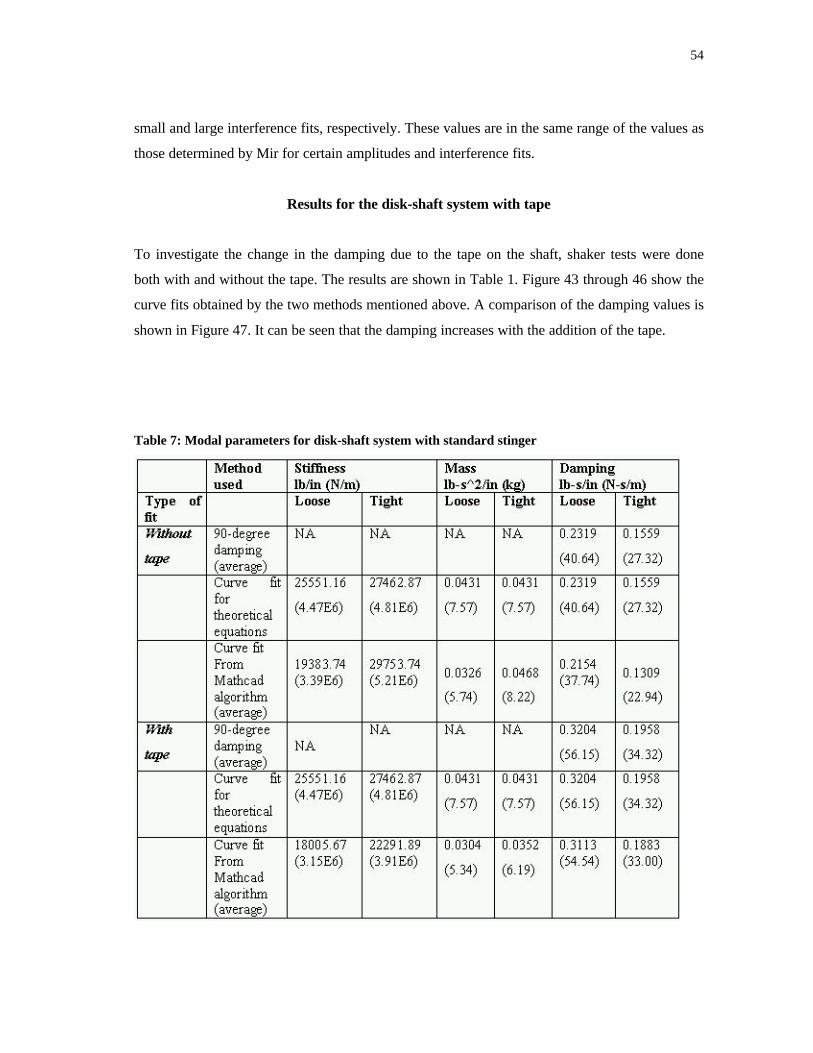
54

small and large interference fits, respectively. These values are in the same range of the values as

those determined by Mir for certain amplitudes and interference fits.

Results for the disk-shaft system with tape

To investigate the change in the damping due to the tape on the shaft, shaker tests were done

both with and without the tape. The results are shown in Table 1. Figure 43 through 46 show the

curve fits obtained by the two methods mentioned above. A comparison of the damping values is

shown in Figure 47. It can be seen that the damping increases with the addition of the tape.

Table 7: Modal parameters for disk-shaft system with standard stinger

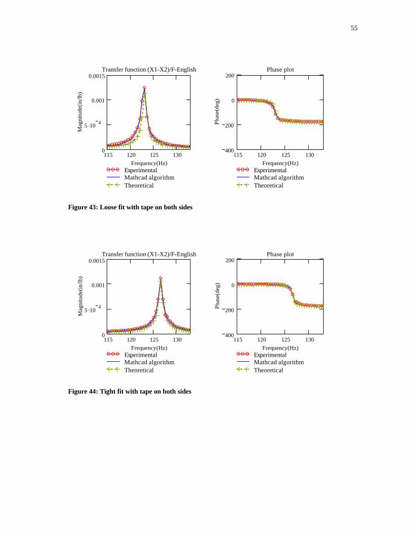
55

115 120 125 1300

5 .10 4

0.001

0.0015

ExperimentalMathcad algorithmTheoretical

Transfer function (X1-X2)/F-English

Frequency(Hz)

Mag

nitu

de(i

n/lb

)

115 120 125 130400

200

0

200

ExperimentalMathcad algorithmTheoretical

Phase plot

Frequency(Hz)

Phas

e(de

g)

Figure 43: Loose fit with tape on both sides

115 120 125 1300

5 .104

0.001

0.0015

ExperimentalMathcad algorithmTheoretical

Transfer function (X1-X2)/F-English

Frequency(Hz)

Mag

nitu

de(i

n/lb

)

115 120 125 130400

200

0

200

ExperimentalMathcad algorithmTheoretical

Phase plot

Frequency(Hz)

Phas

e(de

g)

Figure 44: Tight fit with tape on both sides

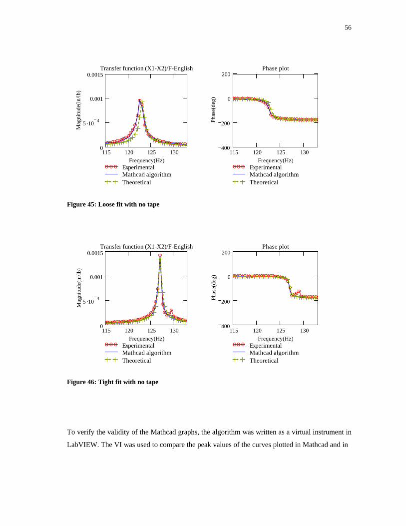
56

115 120 125 1300

5 .10 4

0.001

0.0015

ExperimentalMathcad algorithmTheoretical

Transfer function (X1-X2)/F-English

Frequency(Hz)

Mag

nitu

de(i

n/lb

)

115 120 125 130400

200

0

200

ExperimentalMathcad algorithmTheoretical

Phase plot

Frequency(Hz)

Phas

e(de

g)

Figure 45: Loose fit with no tape

115 120 125 1300

5 .104

0.001

0.0015

ExperimentalMathcad algorithmTheoretical

Transfer function (X1-X2)/F-English

Frequency(Hz)

Mag

nitu

de(i

n/lb

)

115 120 125 130400

200

0

200

ExperimentalMathcad algorithmTheoretical

Phase plot

Frequency(Hz)

Phas

e(de

g)

Figure 46: Tight fit with no tape

To verify the validity of the Mathcad graphs, the algorithm was written as a virtual instrument in

LabVIEW. The VI was used to compare the peak values of the curves plotted in Mathcad and in

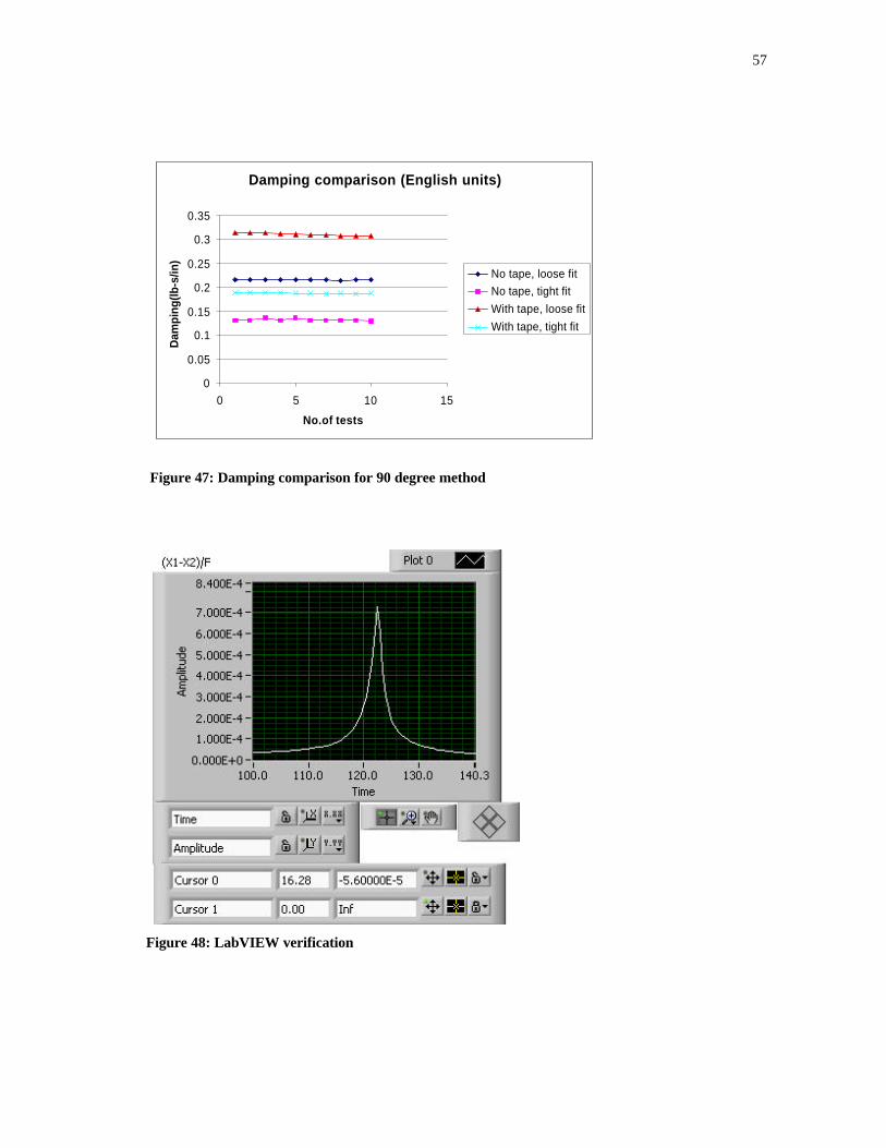
57

Damping comparison (English units)

0

0.05

0.1

0.15

0.2

0.25

0.3

0.35

0 5 10 15

No.of tests

Dam

ping

(lb-s

/in)

No tape, loose fit

No tape, tight fit

With tape, loose fit

With tape, tight fit

Figure 47: Damping comparison for 90 degree method

Figure 48: LabVIEW verification

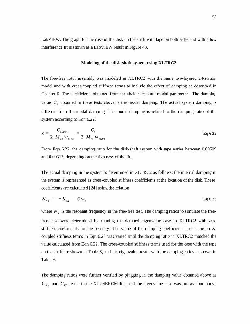
58

LabVIEW. The graph for the case of the disk on the shaft with tape on both sides and with a low

interference fit is shown as a LabVIEW result in Figure 48.

Modeling of the disk-shaft system using XLTRC2

The free-free rotor assembly was modeled in XLTRC2 with the same two-layered 24-station

model and with cross-coupled stiffness terms to include the effect of damping as described in

Chapter 5. The coefficients obtained from the shaker tests are modal parameters. The damping

value iC obtained in these tests above is the modal damping. The actual system damping is

different from the modal damping. The modal damping is related to the damping ratio of the

system according to Eqn 6.22.

( ) ( )2 2Modal i

eq n di eq n di

C C

M Mξ

ω ω= =

⋅ ⋅Eq 6.22

From Eqn 6.22, the damping ratio for the disk-shaft system with tape varies between 0.00509

and 0.00313, depending on the tightness of the fit.

The actual damping in the system is determined in XLTRC2 as follows: the internal damping in

the system is represented as cross-coupled stiffness coefficients at the location of the disk. These

coefficients are calculated [24] using the relation

XY YX nK K C ω= − = Eq 6.23

where nω is the resonant frequency in the free-free test. The damping ratios to simulate the free-

free case were determined by running the damped eigenvalue case in XLTRC2 with zero

stiffness coefficients for the bearings. The value of the damping coefficient used in the cross-

coupled stiffness terms in Eqn 6.23 was varied until the damping ratio in XLTRC2 matched the

value calculated from Eqn 6.22. The cross-coupled stiffness terms used for the case with the tape

on the shaft are shown in Table 8, and the eigenvalue result with the damping ratios is shown in

Table 9.

The damping ratios were further verified by plugging in the damping value obtained above as

XXC and YYC terms in the XLUSEKCM file, and the eigenvalue case was run as done above

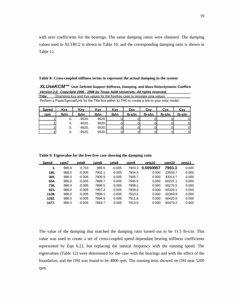
59

with zero coefficients for the bearings. The same damping ratios were obtained. The damping

values used in XLTRC2 is shown in Table 10, and the corresponding damping ratio is shown in

Table 11.

Table 8: Cross-coupled stiffness terms to represent the actual damping in the system

XLUseKCM™ User Defined Support Stiffness, Damping, and Mass Rotordynamic Coefficients

Version 2.0, Copyright 1996 - 1998 by Texas A&M University. All rights reserved.Title: Damping Kxy and Kyx values for the freefree case to simulate zeta values Perform a Paste/Special/Link for the Title box within XLTRC to create a link to your rotor model.

Speed Kxx Kxy Kyx Kyy Cxx Cxy Cyx Cyyrpm lb/in lb/in lb/in lb/in lb-s/in lb-s/in lb-s/in lb-s/in

1 0. -9520. 9520. 0 0 0 0 02 0. -9520. 9520. 0 0 0 0 03 0. -9520. 9520. 0 0 0 0 04 0. -9520. 9520. 0 0 0 0 0

Table 9: Eigenvalue for the free-free case showing the damping ratio

Speed cpm7 zeta8 cpm8 zeta9 cpm9 zeta10 cpm10 zeta11

1. 985.9 0.703 985.9 -0.005 7903.3 0.0050957 7903.3 0.000185. 986.0 -0.005 7902.1 0.005 7904.5 0.000 22603.7 0.000369. 986.0 -0.005 7900.9 0.005 7905.7 0.000 43014.7 0.000554. 986.0 -0.005 7899.7 0.005 7906.9 0.000 60221.1 0.000738. 986.0 -0.005 7898.5 0.005 7908.1 0.000 60270.5 0.000923. 986.0 -0.005 7897.3 0.005 7909.4 0.000 60320.1 0.000

1108. 986.0 -0.005 7896.1 0.005 7910.6 0.000 60369.9 0.0001292. 986.0 -0.005 7894.9 0.005 7911.8 0.000 60420.0 0.0001477. 986.0 -0.005 7893.7 0.005 7913.0 0.000 60470.2 0.000

The value of the damping that matched the damping ratio turned out to be 11.5 lb-s/in. This

value was used to create a set of cross-coupled speed dependant bearing stiffness coefficients

represented by Eqn 6.22, but replacing the natural frequency with the running speed. The

eigenvalues (Table 12) were determined for the case with the bearings and with the effect of the

foundation, and the OSI was found to be 4800 rpm. The running tests showed on OSI near 5200

rpm.

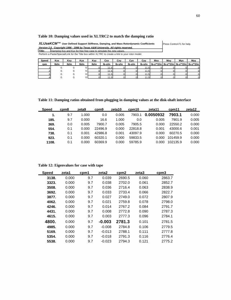
60

Table 10: Damping values used in XLTRC2 to match the damping ratio

XLUseKCM™ User Defined Support Stiffness, Damping, and Mass Rotordynamic Coefficients Press Control-F1 for help.

Version 2.0, Copyright 1996 - 1998 by Texas A&M University. All rights reserved.Title: Damping Kxy and Kyx for free free case to simulate the zeta values.Perform a Paste/Special/Link for the Title box within XLTRC to create a link to your rotor model.

Speed Kxx Kxy Kyx Kyy Cxx Cxy Cyx Cyy Mxx Mxy Myx Myyrpm lb/in lb/in lb/in lb/in lb-s/in lb-s/in lb-s/in lb-s/in lb-s**2/in lb-s**2/in lb-s**2/in lb-s**2/in

1 0. 0. 0. 0 11.5 0 0 11.5 0 0 0 02 0. 0. 0. 0 11.5 0 0 11.5 0 0 0 03 0. 0. 0. 0 11.5 0 0 11.5 0 0 0 04 0. 0. 0. 0 11.5 0 0 11.5 0 0 0 0

Table 11: Damping ratios obtained from plugging in damping values at the disk-shaft interface

Speed cpm8 zeta9 cpm9 zeta10 cpm10 zeta11 cpm11 zeta12

1. 9.7 1.000 0.0 0.005 7903.1 0.0050932 7903.1 0.000

185. 9.7 0.000 16.6 1.000 0.0 0.005 7901.9 0.005369. 0.0 0.005 7900.7 0.005 7905.5 0.000 22550.2 0.000554. 0.1 0.000 22496.9 0.000 22818.8 0.001 43000.6 0.001738. 0.1 0.001 42986.8 0.001 43097.9 0.000 60270.5 0.000923. 0.1 0.000 60320.1 0.000 59833.5 0.000 101459.9 0.000

1108. 0.1 0.000 60369.9 0.000 59785.9 0.000 102135.9 0.000

Table 12: Eigenvalues for case with tape

Speed zeta1 cpm1 zeta2 cpm2 zeta3 cpm33138. 0.000 9.7 0.039 2690.5 0.060 2863.73323. 0.000 9.7 0.038 2702.0 0.061 2852.73508. 0.000 9.7 0.036 2716.4 0.063 2838.93692. 0.000 9.7 0.033 2733.4 0.066 2822.73877. 0.000 9.7 0.027 2749.0 0.072 2807.94062. 0.000 9.7 0.021 2759.8 0.078 2798.04246. 0.000 9.7 0.014 2767.2 0.084 2791.74431. 0.000 9.7 0.008 2772.8 0.090 2787.34615. 0.000 9.7 0.003 2777.3 0.096 2784.1

4800. 0.000 9.7 -0.003 2781.3 0.101 2781.5

4985. 0.000 9.7 -0.008 2784.8 0.106 2779.55169. 0.000 9.7 -0.013 2788.1 0.111 2777.85354. 0.000 9.7 -0.018 2791.3 0.116 2776.45538. 0.000 9.7 -0.023 2794.3 0.121 2775.2

61

The above tests confirmed that the self-bonding tape increases the internal damping in the

system. To further verify the validity of this method, the disk was removed from the shaft and

the shaft was shaken both with and without the tape. The previously described method of

determining the internal damping in a rotor by conducting free-free shaker tests was used.

Shaker tests of the shaft-only system

The shaft was hung free-free and was shaken as was done for the disk-shaft system.

Modeling the shaft system

Since the shaft is a uniform beam, exciting it with a periodic force will excite all its mode shapes

and resulting in an infinite degree of freedom system. But in practice the shaft can be modeled as

a two DOF system as was done for the disk-shaft system.

Determination of modal mass

The shape of the first resonant frequency will be a half sine mode shape with the ends of the

shaft and the center 180 degrees out of phase. The expression for the modal mass is known in

terms of a 2 DOF model, as was shown for the disk-shaft system (Eqn 6.7). The force applied at

the center causes the mass at the center cenm to vibrate with a velocity cenv and the ends of the

shaft with mass endm with a velocity endv . Applying the law of conservation of momentum to

the 2 DOF system model in Figure 45, we get

0cen cen end endm v m v+ = Eq 6.24

Differentiating Eqn 6.21 we get

0cen cen end endm a m a+ = Eq 6.25(a)

which implies that

end cen

cen end

m a

m a= − Eq 6.25(b)

62

The accelerometers measure the values of cena and enda . Solving for cenm and endm from

equations 6.7 and 6.25 (b), and taking into account the difference in phase between cena and

enda to get rid of the negative sign in Eqn 6.25 (b), we get

( )

11cen eq sh

cen

end

m Ma

a

= +

Eq 6. 26

cenend cen

end

am m

a= Eq 6. 27

An XLTRC2 model was created for the shaft, and the resonant frequency of the free-free modes

was correlated with the experimental results. The modal mass of the system was found using Eqn

6.14. Using the modal mass and the ratio of the acceleration at the center to the acceleration at

the end, the values of cenm and endm were determined. The modal mass from XLTRC2 was

obtained as 13.30 lb.

05.6)( =sheqM kg (13.03lb)

Determination of modal stiffness

As done above, the modal stiffness was determined using Eqn 6.16 and was found to be

29.7)( =sheqK MN/m ( 04.41615 lb/in)

Determination of internal damping

The damping was determined using the 90 degree phase shift method and by curve-fitting Eqn

6.12 with the calculated values of modal mass and stiffness to the experimental data and

tweaking the damping value until it matched the peak of the experimental data. A set of

coefficients was also obtained using the curve-fitting function ‘genfit’ in Mathcad. These two

curves were compared with the experimental one.

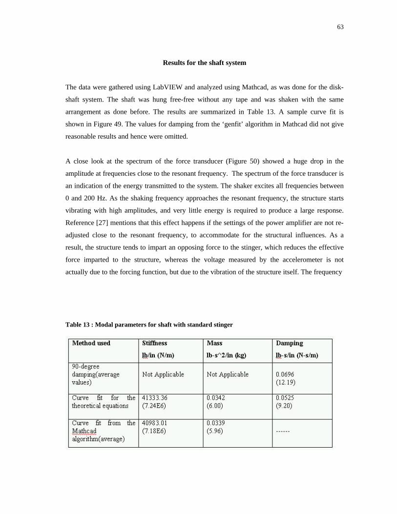
63

Results for the shaft system

The data were gathered using LabVIEW and analyzed using Mathcad, as was done for the disk-

shaft system. The shaft was hung free-free without any tape and was shaken with the same

arrangement as done before. The results are summarized in Table 13. A sample curve fit is

shown in Figure 49. The values for damping from the ‘genfit’ algorithm in Mathcad did not give

reasonable results and hence were omitted.

A close look at the spectrum of the force transducer (Figure 50) showed a huge drop in the

amplitude at frequencies close to the resonant frequency. The spectrum of the force transducer is

an indication of the energy transmitted to the system. The shaker excites all frequencies between

0 and 200 Hz. As the shaking frequency approaches the resonant frequency, the structure starts

vibrating with high amplitudes, and very little energy is required to produce a large response.

Reference [27] mentions that this effect happens if the settings of the power amplifier are not re-

adjusted close to the resonant frequency, to accommodate for the structural influences. As a

result, the structure tends to impart an opposing force to the stinger, which reduces the effective

force imparted to the structure, whereas the voltage measured by the accelerometer is not

actually due to the forcing function, but due to the vibration of the structure itself. The frequency

Table 13 : Modal parameters for shaft with standard stinger

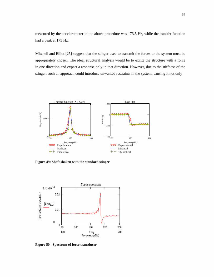
64

measured by the accelerometer in the above procedure was 173.5 Hz, while the transfer function

had a peak at 175 Hz.

Mitchell and Elliot [25] suggest that the stinger used to transmit the forces to the system must be

appropriately chosen. The ideal structural analysis would be to excite the structure with a force

in one direction and expect a response only in that direction. However, due to the stiffness of the

stinger, such an approach could introduce unwanted restraints in the system, causing it not only

170 175 1800

0.005

ExperimentalMathcad Theoretical

Transfer function (X1-X2)/F

Frequency(Hz)

Mag

nitu

de(i

n/lb

)

170 175 180400

200

0

200

ExperimentalMathcadTheoretical

Phase Plot

Frequency(Hz)

Phas

e(de

g)

Figure 49: Shaft shaken with the standard stinger

Figure 50 : Spectrum of force transducer

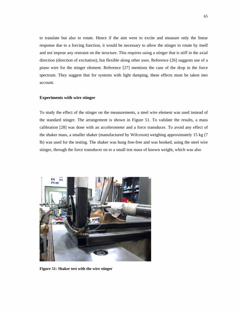
65

to translate but also to rotate. Hence if the aim were to excite and measure only the linear

response due to a forcing function, it would be necessary to allow the stinger to rotate by itself

and not impose any restraint on the structure. This requires using a stinger that is stiff in the axial

direction (direction of excitation), but flexible along other axes. Reference [26] suggests use of a

piano wire for the stinger element. Reference [27] mentions the case of the drop in the force

spectrum. They suggest that for systems with light damping, these effects must be taken into

account.

Experiments with wire stinger

To study the effect of the stinger on the measurements, a steel wire element was used instead of

the standard stinger. The arrangement is shown in Figure 51. To validate the results, a mass

calibration [28] was done with an accelerometer and a force transducer. To avoid any effect of

the shaker mass, a smaller shaker (manufactured by Wilcoxon) weighing approximately 15 kg (7

lb) was used for the testing. The shaker was hung free-free and was hooked, using the steel wire

stinger, through the force transducer on to a small test mass of known weight, which was also

Figure 51: Shaker test with the wire stinger

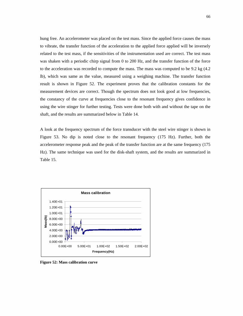
66

hung free. An accelerometer was placed on the test mass. Since the applied force causes the mass

to vibrate, the transfer function of the acceleration to the applied force applied will be inversely

related to the test mass, if the sensitivities of the instrumentation used are correct. The test mass

was shaken with a periodic chirp signal from 0 to 200 Hz, and the transfer function of the force

to the acceleration was recorded to compute the mass. The mass was computed to be 9.2 kg (4.2

lb), which was same as the value, measured using a weighing machine. The transfer function

result is shown in Figure 52. The experiment proves that the calibration constants for the

measurement devices are correct. Though the spectrum does not look good at low frequencies,

the constancy of the curve at frequencies close to the resonant frequency gives confidence in

using the wire stinger for further testing. Tests were done both with and without the tape on the

shaft, and the results are summarized below in Table 14.

A look at the frequency spectrum of the force transducer with the steel wire stinger is shown in

Figure 53. No dip is noted close to the resonant frequency (175 Hz). Further, both the

accelerometer response peak and the peak of the transfer function are at the same frequency (175

Hz). The same technique was used for the disk-shaft system, and the results are summarized in

Table 15.

Mass calibration

0.00E+00

2.00E+00

4.00E+00

6.00E+00

8.00E+00

1.00E+01

1.20E+01

1.40E+01

0.00E+00 5.00E+01 1.00E+02 1.50E+02 2.00E+02

Frequency(Hz)

Mas

s(lb

)

Figure 52: Mass calibration curve

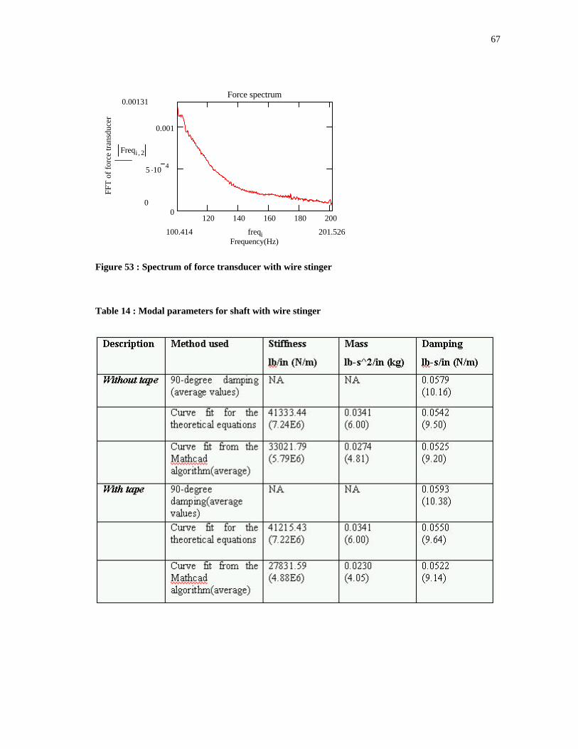
67

120 140 160 180 2000

5 .10 4

0.001

Force spectrum

Frequency(Hz)

FFT

of

forc

e tr

ansd

ucer

0.00131

0

Freqi 2,

201.526100.414 freqi

Figure 53 : Spectrum of force transducer with wire stinger

Table 14 : Modal parameters for shaft with wire stinger

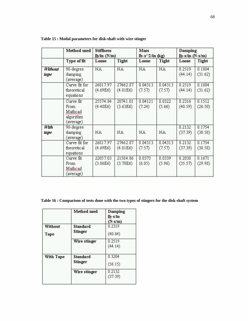
68

Table 15 : Modal parameters for disk-shaft with wire stinger

Table 16 : Comparison of tests done with the two types of stingers for the disk-shaft system

69

Discussion of shaker test results

An attempt has been made to quantify internal friction by conducting shaker tests both on the

disk-shaft system and on the shaft. The internal damping was increased by adding a self-bonding

tape on the shaft. Tests were done both by hanging the shaker and by fixing it on a table. Tests

were also done with the standard metal stinger and with the wire stinger, and the results are

compared in Table 16.

The project depicts a method of determining the internal damping in the system by conducting

shaker tests. Table 1 shows that the addition of the tape increases the internal damping in the

system, and hence gives rise to the subsynchronous frequencies during the running tests,

irrespective of the fit. However, it can be observed that the magnitude of the subsynchronous is

lower in the case of the tight fit, which proves that with the loose fit, the damping effect due to

the fit between the sleeve and the disk also comes into action in addition to the damping due to

the tape.

The experiments with the wire stinger do not give results that match with the predicted values of

equivalent stiffness and mass. The reason for this is not known.

The comparison of the results in Table 16 show that the measured value of the internal damping

does not change much for the case without the tape, regardless of the type of stinger used.

However, the incompatible tests with the tape are presented since the literature suggests the use

of a flexible stinger to avoid moments and back-forces from the shaker to the structure. The fact

that the experimental data for the standard stinger match the equivalent modal mass and stiffness

obtained from using the XLTRC2 model and free-free rap tests gives confidence in believing

those damping values. The signal conditioner for the accelerometers and the force transducer

have a built-in filter for AC biasing, thus avoiding any possible DC offset into the signal that

goes to LabVIEW. The validity of using an accelerometer to get the displacements by dividing

by the square of the frequency was checked by performing a similar experiment on another test

rig that was cantilevered; measurements with the displacements from the accelerometer and a

proximity probe were compared. The measurements from the two tests agreed with each other.

70

CHAPTER VII

SUMMARY AND FUTURE SCOPE

Having investigated experimental methods of determining internal damping in a system, the

principal experimenter next proposes to try differentiating between benign and potentially

harmful vibrations. The measurement of non-destructive subsynchronous vibrations shows that

even though an “instability” is detected, there may be no reason for shutdown of machinery.

Tape was used to create internal friction. However, the practical industry case is assembly

interface that causes the internal friction. Many turbomachines have shrink-fit aluminum wheels

that may be potential sources of instability. To mimic this situation, an aluminum sleeve could

be shrunk fit on the shaft and the shaker and running tests could be conducted. If this system

goes unstable, the filtered orbit of the subsynchronous vibration can be compared with the

filtered orbit for the subsynchronous vibration in other cases, and conclusions can be made based

on the shape of the orbits.

The advantage of probing into the shape of the filtered subsynchronous orbit is that one might be

able to use this for real-time machinery diagnostics, and rather than blindly shutting down a

machine on seeing a subsynchronous component, one might want to analyze it first before

coming to a decision.

From a design point of view, one should bear in mind the possibility of instabilities due to built-

up rotors. Once a rotor is designed and a prototype made, it could be hung free-free and shaken

to determine the internal damping as described above. These results could be incorporated into a

computer simulation to determine if the system will go unstable.

71

REFERENCES

[1] Jeffcott, H.H., 1919, “The Lateral Vibrations of Loaded Shafts in the Neighbourhood of

a Whirling Speed: The Effect of Want of Unbalance”, Philosophical Magazine, Series 6, 37,

pp. 304-318.

[2] Newkirk, B.L., 1925, “Measurement of Internal Friction in a Revolving Deflected

Shaft”, General Electric Review, 28, pp. 554-558.

[3] Kimball, A.L. Jr., 1924, “Internal Friction Theory of Shaft Whirling”, General Electric

Review, 27, pp. 244-251.

[4] Ehrich, F.F., 1964, “Shaft Whirl Induced by Rotor Internal Damping”, Journal of

Applied Mechanics, 31, pp. 279-282.

[5] Gunter, E.J., 1967, “The Influence of Internal Friction on the Stability of High Speed

Rotors”, Journal of Engineering for Industry, (November), 8, pp. 683-688.

[6] Gunter, E.J. Jr., Trumpler, P.R., 1969, “The Influence of Internal Friction on the Stability

of High Speed Rotors with Anisotropic Supports”, Journal of Engineering for Industry,

(November), pp. 1105-1113.

[7] Begg, I.C., “Friction Induced Rotor Whirl – A Study in Stability”, ASME 73-DET -106.

[8] Vance, J.M, Lee, J, 1973, “Stability of High Speed Rotors with Internal Friction”, ASME

Publication, ASME Paper No. 73-DET-127.

[9] Black, H.F., 1976, “The Stabilizing Capacity of Bearings for Flexible Rotors with

Hysteresis”, Journal of Engineering for Industry, (February), pp. 87-91.

[10] Ying, D., Vance, J.M., 1993, “Effect of Press Fits on Threshold Speeds of Rotordynamic

Instability”, TRC Report.

[11] Bently, D.E., Muzsynska, A., 1982, “Rotor Internal Friction Instability”, NASA

Conference Publication, Instability in Rotating Machinery, NAS 1-55-2409, pp. 337-348.

[12] Lund, J.W., 1986, “Destabilization of Rotors from Friction in Internal Joints with

Micro-slip”, Proceedings of the International Conference on Rotordynamics, pp. 487-491,

Tokyo.

[13] Parker, J.S., 1997, “The Development of an Experimental Procedure to Determine the

Amount of Active Internal Damping in a Rotor-Bearing System”, M.S. Thesis, Texas A&M

University.

72

[14] Bently, D.E., 1972, “The Re-Excitation of Balance Response Regions by Internal

Friction: Kimball Revisited”, ASME Paper No. 72-Pet-49.

[15] Albaz.K., 2000, “Effect of Shrink Fits on Threshold Speeds of Rotordynamic

Instability”, M.S. Thesis, Texas A&M University, December.

[16] Mir.M., 2001, “Effect of Shrink Fits on Threshold Speeds of Rotordynamic Instability”,

M.S. Thesis, Texas A&M University, December.

[17] Steidel, R.F. Jr., 1988, An Introduction to Mechanical Vibrations, John Wiley and Sons,

New York, 3rd edition.

[18] Shaw, J., Shaw, S.W., 1989, “Instabilities and Bifurcation in a Rotating Shaft”, Journal

of Sound and Vibration, 132, pp 227-244.

[19] Ferrara, P.L., 1977, “Vibrations in a Very High pressure Centrifugal Compressor”,

ASME Paper No. 77-DET-15.

[20] Gunter, E.J., Kirk, R.G., 1975, “Stability and Transient Motion of a Plain Journal

Mounted in Flexible Damped Supports”, ASME Paper No. 75-DET-116.

[21] Murphy, B.T., 1984, “Eigenvalues of Rotating Machinery”, Ph.D. Dissertation, Texas

A&M University, May.

[22] Xu, J., “Rotor Foundation Dynamics for Improved Prediction of Critical Speeds”, report

(available from Dr. John Vance, Texas A&M University), April 1998.

[23] Lin, Y.Q., 1993, “Rotor Instability Induced by Radial Clearance in Ball Bearing

Supports”, ASME Paper No. 93-GT-29.

[24] Vance, J.M., 1988, Rotordynamics of Turbomachinery, John Wiley and Sons, New

York.

[25] Mitchell, L.D., Elliott K.B., 1984, “How to Design Stingers for vibration Testing of

Structures”, Sound and Vibration, (April), 18, pp. 14-18.

[26] Maia, N.M.M, Silva, J.M.M et al, 1997, Theoretical and Experimental Modal Analysis,

John Wiley and Sons, New York.

[27] Mitchell, L.D., Mitchell, L.D., 1985, “Wrong with Confidence, Analyzer Problems”,

Proceedings of the 1985 ASME fall Conference on Experimental Mechanics, pp. 120-128.

[28] Ewins D.J., 1984, Modal Testing, Theory and Practice, John Wiley and Sons, New

York.

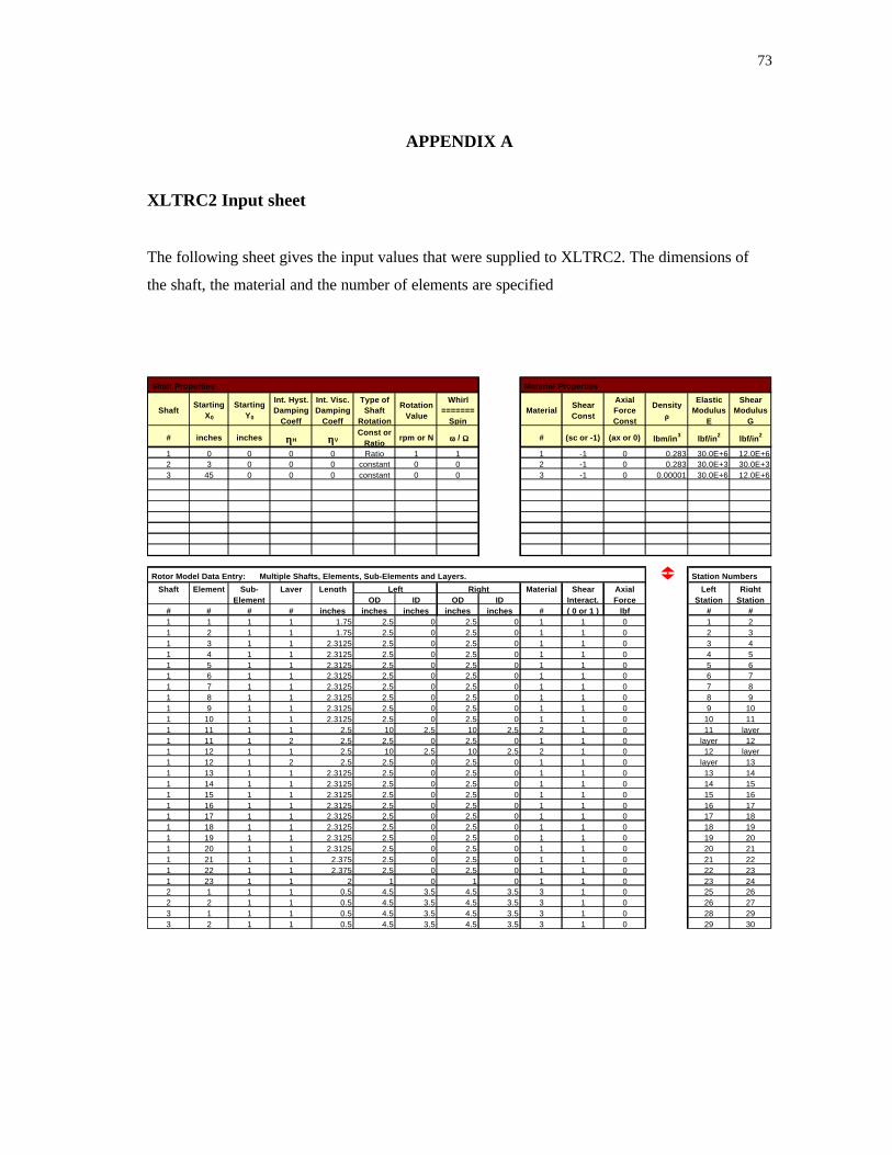
73

APPENDIX A

XLTRC2 Input sheet

The following sheet gives the input values that were supplied to XLTRC2. The dimensions of

the shaft, the material and the number of elements are specified

Shaft Properties Material Properties

ShaftStarting

X0

Starting Y0

Int. Hyst. Damping

Coeff

Int. Visc. Damping

Coeff

Type of Shaft

Rotation

Rotation Value

Whirl =======

SpinMaterial

Shear Const

Axial Force Const

Density ρρ

Elastic Modulus

E

Shear Modulus

G

# inches inches ηηH ηηVConst or

Ratiorpm or N ωω / Ω Ω # (sc or -1) (ax or 0) lbm/in3 lbf/in2 lbf/in2

1 0 0 0 0 Ratio 1 1 1 -1 0 0.283 30.0E+6 12.0E+62 3 0 0 0 constant 0 0 2 -1 0 0.283 30.0E+3 30.0E+33 45 0 0 0 constant 0 0 3 -1 0 0.00001 30.0E+6 12.0E+6

Rotor Model Data Entry: Multiple Shafts, Elements, Sub-Elements and Layers. Station Numbers

Shaft Element Sub- Layer Length Left Right Material Shear Axial Left RightElement OD ID OD ID Interact. Force Station Station

# # # # inches inches inches inches inches # ( 0 or 1 ) lbf # #1 1 1 1 1.75 2.5 0 2.5 0 1 1 0 1 21 2 1 1 1.75 2.5 0 2.5 0 1 1 0 2 31 3 1 1 2.3125 2.5 0 2.5 0 1 1 0 3 41 4 1 1 2.3125 2.5 0 2.5 0 1 1 0 4 51 5 1 1 2.3125 2.5 0 2.5 0 1 1 0 5 61 6 1 1 2.3125 2.5 0 2.5 0 1 1 0 6 71 7 1 1 2.3125 2.5 0 2.5 0 1 1 0 7 81 8 1 1 2.3125 2.5 0 2.5 0 1 1 0 8 91 9 1 1 2.3125 2.5 0 2.5 0 1 1 0 9 101 10 1 1 2.3125 2.5 0 2.5 0 1 1 0 10 111 11 1 1 2.5 10 2.5 10 2.5 2 1 0 11 layer1 11 1 2 2.5 2.5 0 2.5 0 1 1 0 layer 121 12 1 1 2.5 10 2.5 10 2.5 2 1 0 12 layer1 12 1 2 2.5 2.5 0 2.5 0 1 1 0 layer 131 13 1 1 2.3125 2.5 0 2.5 0 1 1 0 13 141 14 1 1 2.3125 2.5 0 2.5 0 1 1 0 14 151 15 1 1 2.3125 2.5 0 2.5 0 1 1 0 15 161 16 1 1 2.3125 2.5 0 2.5 0 1 1 0 16 171 17 1 1 2.3125 2.5 0 2.5 0 1 1 0 17 181 18 1 1 2.3125 2.5 0 2.5 0 1 1 0 18 191 19 1 1 2.3125 2.5 0 2.5 0 1 1 0 19 201 20 1 1 2.3125 2.5 0 2.5 0 1 1 0 20 211 21 1 1 2.375 2.5 0 2.5 0 1 1 0 21 221 22 1 1 2.375 2.5 0 2.5 0 1 1 0 22 231 23 1 1 2 1 0 1 0 1 1 0 23 242 1 1 1 0.5 4.5 3.5 4.5 3.5 3 1 0 25 262 2 1 1 0.5 4.5 3.5 4.5 3.5 3 1 0 26 273 1 1 1 0.5 4.5 3.5 4.5 3.5 3 1 0 28 293 2 1 1 0.5 4.5 3.5 4.5 3.5 3 1 0 29 30

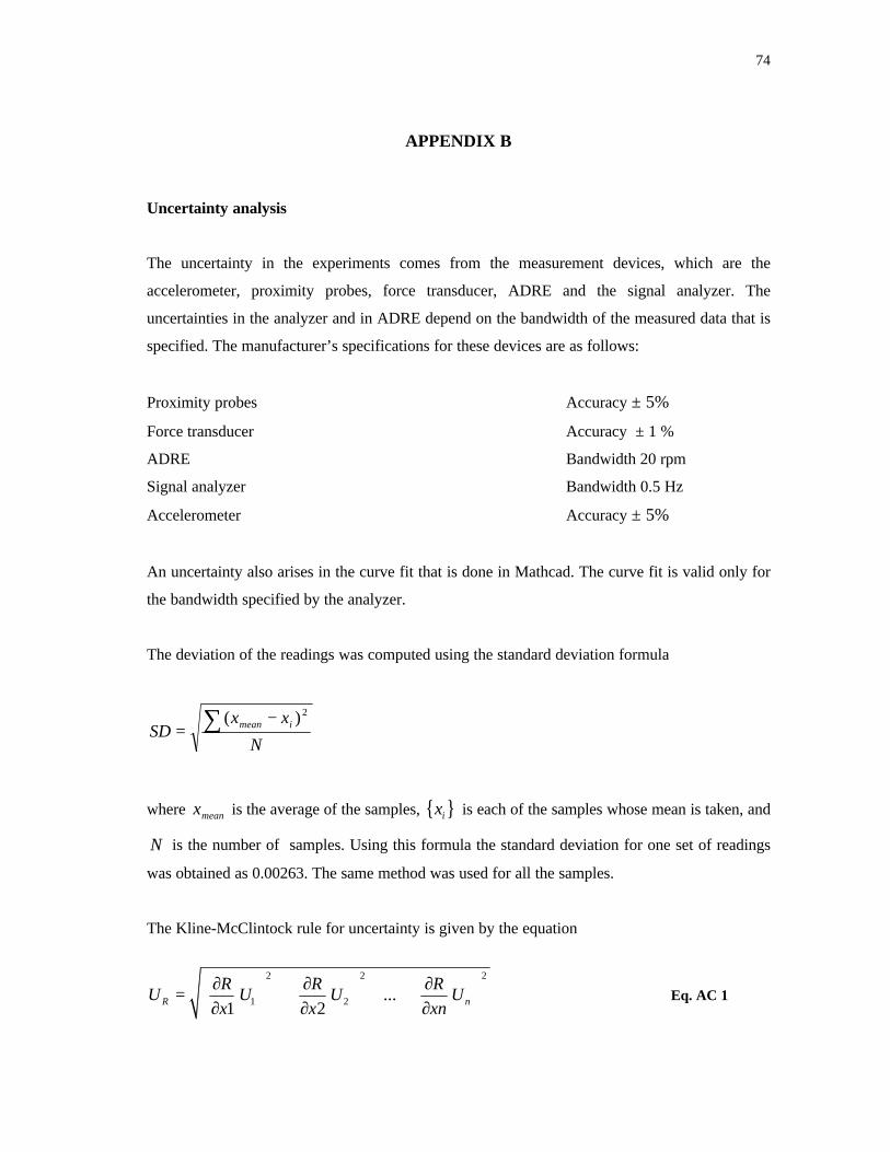
74

APPENDIX B

Uncertainty analysis

The uncertainty in the experiments comes from the measurement devices, which are the

accelerometer, proximity probes, force transducer, ADRE and the signal analyzer. The

uncertainties in the analyzer and in ADRE depend on the bandwidth of the measured data that is

specified. The manufacturer’s specifications for these devices are as follows:

Proximity probes Accuracy ± 5%

Force transducer Accuracy ± 1 %

ADRE Bandwidth 20 rpm

Signal analyzer Bandwidth 0.5 Hz

Accelerometer Accuracy ± 5%

An uncertainty also arises in the curve fit that is done in Mathcad. The curve fit is valid only for

the bandwidth specified by the analyzer.

The deviation of the readings was computed using the standard deviation formula

N

xxSD imean∑ −

=2)(

where meanx is the average of the samples, ix is each of the samples whose mean is taken, and

N is the number of samples. Using this formula the standard deviation for one set of readings

was obtained as 0.00263. The same method was used for all the samples.

The Kline-McClintock rule for uncertainty is given by the equation

2 2 2

1 2 ...1 2R n

R R RU U U U

x x xn

∂ ∂ ∂ = + + + ∂ ∂ ∂ Eq. AC 1

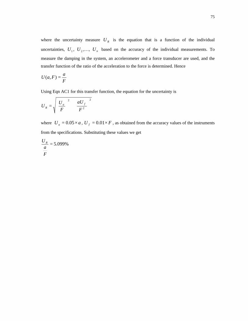
75

where the uncertainty measure RU is the equation that is a function of the individual

uncertainties, 1U , 2U ,…, nU based on the accuracy of the individual measurements. To

measure the damping in the system, an accelerometer and a force transducer are used, and the

transfer function of the ratio of the acceleration to the force is determined. Hence

F

aFaU =),(

Using Eqn AC1 for this transfer function, the equation for the uncertainty is

2

2

2

+

=

F

aU

F

UU fa

R

where aU a ×= 05.0 , FU f ×= 01.0 , as obtained from the accuracy values of the instruments

from the specifications. Substituting these values we get

%099.5=

F

aU R

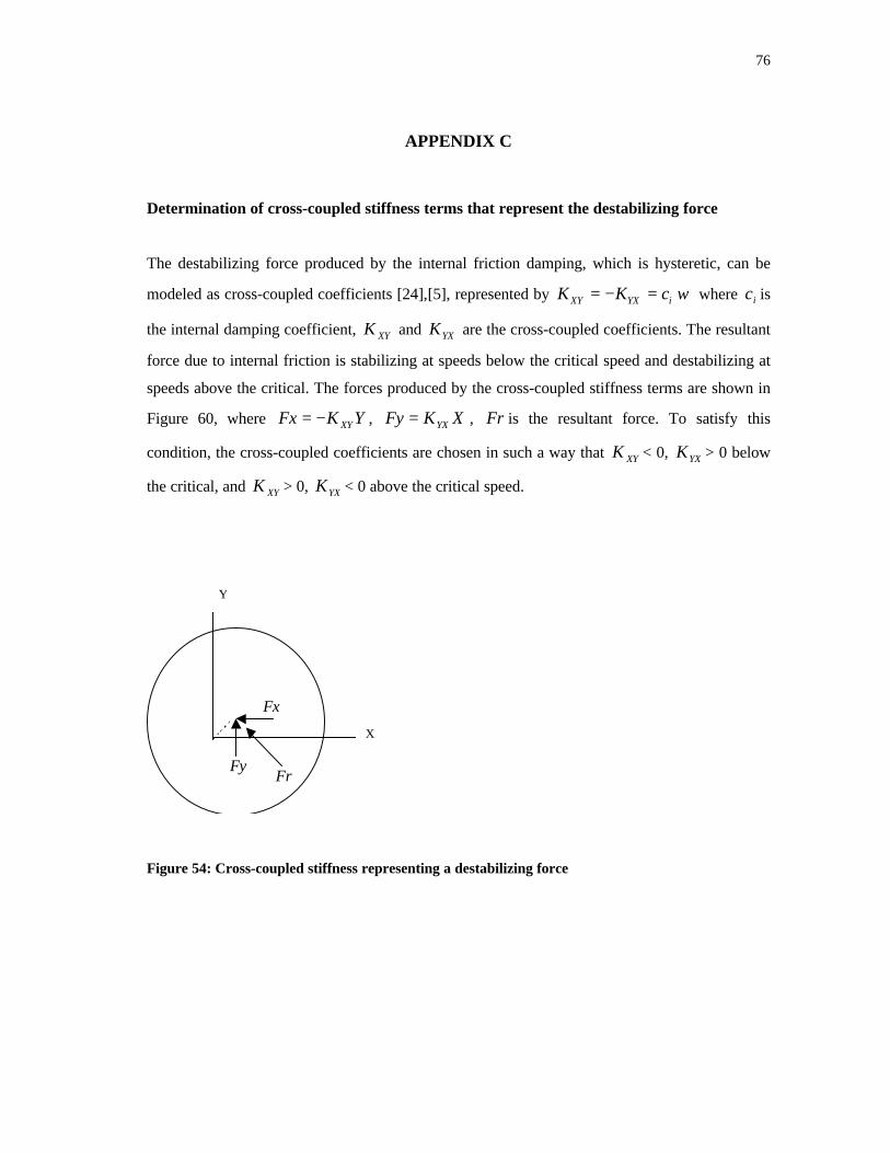
76

APPENDIX C

Determination of cross-coupled stiffness terms that represent the destabilizing force

The destabilizing force produced by the internal friction damping, which is hysteretic, can be

modeled as cross-coupled coefficients [24],[5], represented by XY YX iK K c ω= − = where ic is

the internal damping coefficient, XYK and YXK are the cross-coupled coefficients. The resultant

force due to internal friction is stabilizing at speeds below the critical speed and destabilizing at

speeds above the critical. The forces produced by the cross-coupled stiffness terms are shown in

Figure 60, where YKFx XY−= , XKFy YX= , Fr is the resultant force. To satisfy this

condition, the cross-coupled coefficients are chosen in such a way that XYK < 0, YXK > 0 below

the critical, and XYK > 0, YXK < 0 above the critical speed.

X

Y

Fr

Fx

Fy

Figure 54: Cross-coupled stiffness representing a destabilizing force

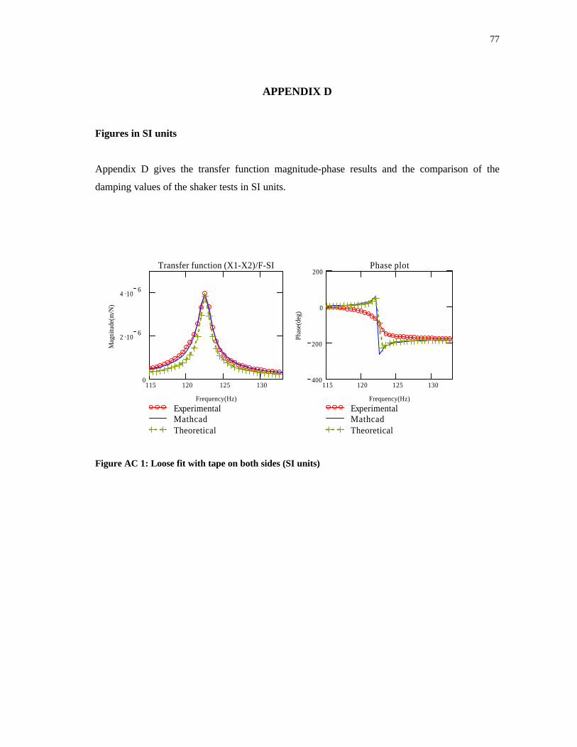
77

APPENDIX D

Figures in SI units

Appendix D gives the transfer function magnitude-phase results and the comparison of the

damping values of the shaker tests in SI units.

115 120 125 1300

2 .106

4 .106

ExperimentalMathcadTheoretical

Transfer function (X1-X2)/F-SI

Frequency(Hz)

Mag

nitu

de(m

/N)

115 120 125 130400

200

0

200

ExperimentalMathcadTheoretical

Phase plot

Frequency(Hz)

Phas

e(de

g)

Figure AC 1: Loose fit with tape on both sides (SI units)

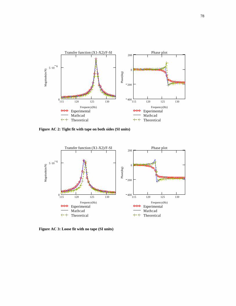
78

115 120 125 1300

5 .106

ExperimentalMathcadTheoretical

Transfer function (X1-X2)/F-SI

Frequency(Hz)

Mag

nitu

de(m

/N)

115 120 125 130400

200

0

200

ExperimentalMathcadTheoretical

Phase plot

Frequency(Hz)

Phas

e(de

g)

Figure AC 2: Tight fit with tape on both sides (SI units)

115 120 125 1300

5 .106

ExperimentalMathcadTheoretical

Transfer function (X1-X2)/F-SI

Frequency(Hz)

Mag

nitu

de(m

/N)

115 120 125 130400

200

0

200

ExperimentalMathcadTheoretical

Phase plot

Frequency(Hz)

Phas

e(de

g)

Figure AC 3: Loose fit with no tape (SI units)

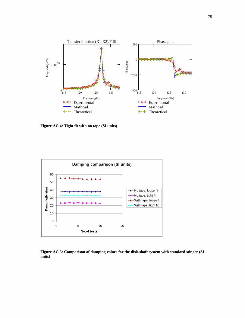
79

115 120 125 1300

5 .106

ExperimentalMathcadTheoretical

Transfer function (X1-X2)/F-SI

Frequency(Hz)

Mag

nitu

de(m

/N)

115 120 125 130400

200

0

200

ExperimentalMathcadTheoretical

Phase plot

Frequency(Hz)

Phas

e(de

g)Figure AC 4: Tight fit with no tape (SI units)

Damping comparison (SI units)

0

10

20

30

40

50

60

0 5 10 15

No.of tests

Dam

ping

(N-s

/m)

No tape, loose fit

No tape, tight fit

With tape, loose fit

With tape, tight fit

Figure AC 5: Comparison of damping values for the disk-shaft system with standard stinger (SIunits)

80

VITA

ANAND SRINIVASANPlot 58, Door 5/2, Rajaram Salai, K.K.Nagar, Trichy 620021, INDIA.

Ph: 91-431-2459293; anand_s78@yahoo.com

EDUCATION

Texas A&M University, College Station, TX Sep 2000 – May 2003Master of Science in Mechanical Engineering, Degree GPA: 3.5/4.0

University of Madras, Chennai, India Aug 1996 - May 2000Bachelor of Engineering, Mechanical Engineering Overall GPA 3.96/4.00

EXPERIENCE

Research Assistant, Turbomachinery Laboratory, Texas A&M University Sep 2000 – May 2003

• Working under Prof. John Vance, involved in experimental static (determination ofrotordynamic coefficients – stiffness, mass, damping) and dynamic analyses (response ofmachinery to excitation forces – collection and interpretation of Bode, Waterfall plots) oftest rigs.

• Was involved in the hardware construction (piping for lube lines, foundation, electricalsupplies) and commissioning of the General Electric 7HDL Turbocharger for testingpurpose.

Lucas TVS, Chennai, India May 1997

Underwent an Internship in the maintenance department in this leading automotive startermanufacturing company and learned various skills concerning manufacturing processes.

COMPUTER SKILLS

• Worked with programming languages such as BASIC, FORTRAN90, C, Excel Visual Basic• Proficient in SolidWorks, a Solid Modeling package and COSMOS, a finite element analysis

package; Experience in Pro Engineer 2000i and Auto CAD• Knowledge of XLTRC, an Excel based modeling software for rotating machinery and

ADRE, a data acquisition system• Fluent usage of packages such as MS Word, MS Excel, MS PowerPoint, MS FrontPage,

Adobe Photoshop• Experience in Maple, MATLAB, MathCAD, LABVIEW• Knowledge of Cambridge Engineering Selector, a material and process selection tool