REVIEW OF JOOST KALKER’S WHEEL-RAIL CONTACT THEORIES

Proceedings of the ASME 2009 International Design Engineering Technical Conference & Computers and Information in Engineering Conference

IDETC/CIE 2009 August 30-September 2, 2009, San Diego, California, USA

DETC-87655

REVIEW OF JOOST KALKER’S WHEEL-RAIL CONTACT THEORIES AND THEIR IMPLEMENTATION IN MULTIBODY CODES

Khaled E. Zaazaa

ENSCO, Inc. 5400 Port Royal Road,

Springfield VA 22151, USA [email protected]

A. L. Schwab Delft University of Technology

Laboratory for Engineering Mechanics, Mekelweg 2, NL 2628 CD Delft, The Netherlands

[email protected]

ABSTRACT During the past decades Kalker developed a number of wheel-rail contact theories that can be used to determine the tangential forces and spin moment between the wheel and the rail [Kalker, 1990]. These theories are: Linear Theory, Strip Theory, Empirical Theory, Simplified Theory and Exact Three Dimensional Rolling Contact Theory. These theories assume that the contact between the two bodies is non-conformal. Recently, Li and Kalker [Li and Kalker 1998a, 1998b and Li, 2002] introduced an approach for numerical solution of the conformal contact between the wheel and the rail. In this paper, Kalker’s wheel-rail contact theories are presented. The paper provides an overview for each theory and its restriction or error as was reported by Kalker. In addition, a systematic procedure for implementing Kalkers’s wheel-rail contact theories in multibody codes is briefly presented.

INTRODUCTION In 1951, Joost J. Kalker entered Delft University of technology as a student of physics. Shortly after, he was transferred to applied mechanics to start his researches on contact mechanics, computers and programming. In 1958, Kalker graduated as mathematical engineer. During this period, De Pater introduced Kalker to wheel-rail contact problem. In 1967, Kalker was awarded his PhD degree. His PhD dissertation, “On the Rolling Contact of Two Elastic Bodies in the Presence of Dry Friction”, introduced Kalker’s creep forces linear theory [Kalker, 1967a]. In this theory, the contact patch is divided into an adhesion and sliding area and the effect of the spin moment is included. The theory is based on the assumption that the traction distribution is continuous at the leading edge of the contact. That is the traction must vanish at the leading edge

where the particles enter the contact area. On the other hand within the contact area, the traction builds up until the trailing edge. In addition, Kalker introduced the table of creepage and spin coefficients that are known as Kalker’s coefficients [Kalker, 1967a]. Kalker’s coefficients are used in several wheel-rail contact theories to determine the tangential forces and spin moment. To this day, the linear theory is commonly used to investigate railroad vehicle dynamics.

In 1964-1967, Kalker extended the original Strip Theory developed by [Haines and Ollerton, 1963] by employing the lateral and spin creepages in addition to the longitudinal creepage. In this theory, the area of contact is assumed to be elliptical with long lateral semi-axis. Kalker [Kalker, 1964b, 1964a, 1967a and 1972] proved that, for such contact area, the area of contact can be divided into slices parallel to the longitudinal axis of the contact area. In each slice, Carter theory [Carter, 1926] can be used to determine the tangential force. The strip theory was replaced by the Simplified Theory due to its limitation to slender contact area. Therefore, it will not be presented in this paper.

In 1968, Kalker introduced the Empirical Theory [Kalker, 1968b]. This theory defines the relation between the longitudinal and lateral creepages and total creep force. Kalker’s empirical theory is more accurate compared to the empirical theory proposed by Johnson and Vermeulen in 1964 [Johnson and Vermeulen, 1964].

During the period of 1973-1982, Kalker developed the Simplified Theory [Kalker 1973, 1981, and 1982]. The theory is based on approximating the relation between the tangential surface traction and the tangential surface displacement by using compliant (flexibility) parameters. These compliant parameters depend on the creepage and spin coefficients of the

1 Copyright © 2009 by ASME

Proceedings of the ASME 2009 International Design Engineering Technical Conferences & Computers and Information in Engineering Conference

IDETC/CIE 2009 August 30 - September 2, 2009, San Diego, California, USA

DETC2009-87655

mailto:[email protected]

mailto:[email protected]

linear theory. This theory is used in well known program FASTSIM that was developed by Kalker in 1982 [Kalker, 1982]. FASTSIM is widely used in computer programs to determine the wheel-rail creep contact forces.

In 1986, Kalker generalized the principal of virtual work for solving the contact problem [Kalker, 1986b and 1986c]. The use of the principle of virtual work led to the Exact Three-Dimensional Rolling Contact Theory. In this theory, the solution of the contact problem is determined by maximizing the complementary work over all possible functions that satisfy the constraints. In addition, the displacements of the surface in the contact area are expressed as integrals of the surface tractions by using influence functions [Kalker, 1990]. The influence functions can be determined analytically for the homogenous, isotropic half-space. Therefore, half-space assumption is used in this theory. The exact three dimensional rolling contact theory is used in the well known program CONTACT developed by Kalker.

To this end, the methods described in the preceding paragraphs assume that the contact area is non-conformal, and the half-space approximation is utilized. In the case of conformal contact, the half-space approximation is no longer valid as the size of the contact area is not small compared to the size of the contacting bodies. In addition, the creepages and spin are not constant within the contact area. Li and Kalker used two quasi-quarter spaces for solving the conformal contact problem [Li and Kalker 1998a, 1998b and Li, 2002]. In their approach, the variation of spin throughout the contact area is considered. This paper is organized as follows: in section 2, the wheel-rail contact problem is briefly introduced. The mathematical representations of the wheel-rail rolling contact problem and the definitions and terminologies that will be used in this paper are presented in this section. In section 3, the linear theory is presented. The limitations of the linear theory are discussed in this section. In section 4, the empirical theory that can be used for special cases is presented. In section 5, the simplified theory is introduced. The presentation of the simplified theory, in this section, is used to briefly describe the algorithm of the FASTSIM program. In section 6, the exact three dimensional rolling contact theory is discussed. The method of virtual work that is used to drive this theory is presented in this section. In section 7, the conformal contact problem is briefly described. The Li-Kalker theory for conformal contact is presented in this section. In section 8, a systematic approach for implementing Kalker’s wheel-rail contact theories in multibody codes is described. The procedure uses non-generalized surface parameters to represent the wheel and the rail surfaces [Shabana, et al, 2008]. Some results that are obtained from a multibody code are presented in this paper. Finally, summary and discussions of the Kalker’s wheel-rail contact theories are provided in section 9.

WHEEL-RAIL ROLLING CONTACT PROBLEM Due to the elasticity of the wheel and the rail and the externally applied load, some points on the surfaces in the contact region may slip while others may stick when the two bodies move relative to each other. The difference between the tangential strains of the bodies in the adhesion area leads to small apparent slip (creepage). Creepages generate tangential creep forces and spin moment. In the case of wheel-rail contact, tangential forces and spin moment are generated, since the motion of the wheel relative to the rail is a combination of rolling and sliding.

In case of a wheel rolling on a rail, the rail coordinate system is defined by the fixed Cartesian coordinate system r r rX Y Z , as shown in Fig. 1. If the wheel rolls over the rail in the direction of positive rX with a rolling velocity vector of the wheel center , the magnitude of the rolling velocity is defined as

vV = v . In addition, a coordinate

system, X Y Z , which moves with the contact point can be used so that rX X Vt= − , where t is the time. In the point of contact, the wheel has a circumferential velocity c , relative to the wheel center, that is almost opposite to the rolling velocity

in the point of contact. Therefore, a rigid slip can be defined as the sum of these velocities as follows: v

= +s v c& (1) Clearly, the rigid slip is defined in the tangential plane and represents the effect of the velocity in this plane and the rotation about the Z-axis as follows [Kalker, 1979b and 1980]:

( ) ( )x yV y xξ ϕ ξ ϕ⎡ ⎤= + = − + +⎣ ⎦s v c i j& (2)

where and i j are the unit vectors along X and directions, respectively,

Yxξ and yξ are the longitudinal and lateral

creepage, respectively, and ϕ is the spin creepage. The longitudinal, lateral and spin creepages are defined as follows [Kalker, 1980]:

( ) ,

,sincos

x

y

V

V R

ξ

ξ αα γϕ γ

⎫= − ⎪

⎪= ⎬

⎪⎪= − +⎭

v c

&

(3)

where α is the angle between the wheel plane and the plane Y = 0 and R and γ are the wheel rolling radius and the wheel conicity, respectively, as shown in Fig. 2.

Figure 1. Wheel rolling over a rail.


Due to the elasticity of the wheel and the rail and the

externally applied load, the two bodies will deform and touch along an elliptical contact area according to Hertz’s theory [Hertz, 1882]. In this case, the normal pressure exerted on the wheel and the rail is defined as follows:

( ) ( )23( , ) 12

Np x y x a y babπ

= − − 2 (4)

where a and b are the contact area semi-axes and N is the normal applied force.

Y

Z

Y

Z

Figure 2. Direction of velocity.

The displacement of a particle of the wheel is different

than the displacement of a particle of the rail due the local deformations of the wheel and the rail in the area of contact. This difference is given by

w r= −u u u (5) where and are the surface displacement of the wheel and the rail in the tangential plane (X,Y), respectively. The true slip can be defined as the sum of the rigid slip given by Eq. 2 and the time derivative of the relative displacement of the material given by Eq. 5 as follows [Kalker, 1979b and 1980]:

wu ru

( ) ( ) ( ) (( , ) ( , , )

/ /x y

x y x y t

V y x V xξ ϕ ξ ϕ

= +

⎡ ⎤= − + + − ∂ ∂ + ∂ ∂⎣ ⎦

w s u

i j u u

&& &

)t (6)

In case of steady state rolling, ( . )/ 0t∂ ∂ =uThe preceding tangential slip defined on the contact

plane can be used to define the tangential traction using Coulomb’s law as

tF

; 0 (adhesion are

; 0 (slip ar

Tt tx ty

t

F F p

p

µ

µ

⎫⎡ ⎤= ≤ = a)

ea)

⎪⎣ ⎦ ⎪⎬⎪= − ≠⎪⎭

F w

wF ww

&

&&

&

(7)

where µ is the friction coefficient and is the contact pressure and

p

txF and tyF are the longitudinal and lateral creep forces per unit area, respectively. Therefore, the total longitudinal, lateral creep forces and spin creep moment can be expressed as follows:

( )

x tx

y ty

ty tx

F F dx dy

F F dx dy

M xF yF dx dyϕ

⎫=⎪⎪

= ⎬⎪⎪= −⎭

∫∫∫∫∫∫

(8)

The creep forces and the spin moment depend on the creepages, the contact ellipse dimension, and the normal force. The relationship between the longitudinal, lateral and spin creepages and the longitudinal and lateral forces and spin moments are governed by the creep-force law [Kalker, 1977a, 1977b, 1979b, 1980, 1986a and 1990]. Kalker’s creep-forces theories are discussed in the following sections. LINEAR THEORY During the period of 1957-1972, Kalker developed the Linear Theory. The linear theory was based on the work originated by De Pater in 1956 [Kalker, 1979b and 1980 and Kalker and De Pater, 1971]. The linear theory assumes that the true slip, Eq. 6, vanishes. That is ( , ) 0x y =w& . This assumption is based on the effect of the applied pressure is ignored at the edges of the contact area. The linear theory uses the well known Kalker coefficients and , to determine the relation between the creepages and the creep forces and moment. Then, the creep forces and spin moment can be expressed in the matrix form as follows [Kalker, 1967a]:

11 23 22, ,C C C 33C

11

22 23

23 33

0 0

0

0

x x

y y

z

CFF Gab C abCM abC abC

ξξϕ

⎡ ⎤⎡ ⎤ ⎡⎢ ⎥

⎤⎢ ⎥ ⎢= − ⎢ ⎥

⎥⎢ ⎥ ⎢

⎢ ⎥⎥

⎢ ⎥ ⎢− ⎥⎣ ⎦ ⎣⎣ ⎦ ⎦

(13)

In 1956, De Pater assumed that for the case of circular contact area ( a b= ) and a Poisson ratio 0ν = , the can be determined analytically. In 1957, Kalker relaxed the assumption of the circular contact area (

11C

a b≠ ) and determined all coefficients. In 1958, Kalker determined all coefficients in case a b≠ and 0ν ≠ [Kalker, 1958, 1964a, 1966, 1967a , 1968a, 1969 and 1970]. Using the line contact theory, Kalker extend the calculation of the coefficient for the case where

0a b → or 0b a → [Kalker, 1972]. The derivation of the linear theory depends on the steady state assumption. Therefore, Eq. 6 can be expressed as follows:

( ) ( ) ( )( , ) ( , , ) x yx y x y t V y x Vξ ϕ ξ ϕ⎡ ⎤ x= + = − + + − ∂⎣ ⎦w s u i j u&& & ∂

(14) or

( )( )

x x x

y y y

w V y u x

w V x u x

ξ ϕ

ξ ϕ

= − − ∂ ∂ ⎫⎪⎬

= + − ∂ ∂ ⎪⎭ (15)

To determine the creep forces and moment given by Eq. 8, the following conditions are assumed [Kalker, 1967a]:

1. The stresses and displacement vanish at infinity, 2. The contact area is elliptical and the normal pressure

inside the contact area is given by

( ) ( )2 23( , ) 12

Np x y x a y babπ

= − −


3. The tangential tractions vanish outside the contact area,

4. The true slip vanishes in the region of adhesion in the contact area. That is , therefore, 0x yw w= =

( )( )

x x

y y

u x y

u x x

ξ ϕ

ξ ϕ

∂ ∂ = − ⎫⎪⎬

∂ ∂ = + ⎪⎭

5. Integrating the preceding equation w.r.t. x , one gets

1( )x xu x yx D yξ ϕ= + + , and 22

1 ( )2y yu x x Dξ ϕ= + + y

where and are arbitrary functions in y. These functions are determined by assuming the traction distribution is continuous at the leading edge of the contact as shown in Fig. 3. That is the traction must vanish at the leading edge where the particles enter the contact area. Within the contact area, the traction builds up until the trailing edge as shown in Fig. 3.

1( )D y 2 ( )D y

Figure 3. Traction distribution within the contact area for

Kalker’s linear theory. Kalker determined the values of the coefficients , and as functions of the ratio of the contact ellipse semi-axes and Poisson’s ratio [Kalker, 1967a and 1990]. It is important to mention that, the linear theory is valid if the material properties of the two bodies are the same. However, Kalker [Kalker, 1990] proposed the following expressions for the combined material properties of the two bodies:

11 22,C C 23C 33C

( ) ( ) ( )11 1 12

w rG G G⎡= +⎣ ⎤⎦ , (16)

( ) ( ) (12

w w r rG Gν ν ν⎡ ⎤= +⎣ ⎦)G (17)

where and are the modulus of rigidity of the wheel and the rail, respectively, and

wG rGwν and rν are the Poisson’s ratio of

the wheel and the rail respectively. To this end, the main drawback of the linear theory is its limitation to handle large spin and large creepages. In addition, the condition t pµ≤F is violated at the trailing edge where the wheel and rail particles leave the contact area. EMPIRICAL THEORY In 1968, Kalker introduced the empirical theory [Kalker, 1968b]. This theory defines the relation between the

longitudinal and lateral creepages and total creep force. The theory states that the total creep force is given as follows:

1 1 2 2

2

( ) ( ) 1,1,

f fN

τ τ ττµ

+ ≤⎧= ⎨ ≥⎩

e eFe

(18)

and 2 2τ ξ η= +

3xabG Nξ π ξ µ φ= , 3yabG Nη π ξ µ ψ=

11

3( ) cos2

f τ τ τ−= , 2 22

1( ) 1 1 12

f τ τ τ⎛ ⎞= − + −⎜ ⎟⎝ ⎠

( )1 ξ η τ= +e i j , ( ) 2 22 x y x yξ ξ ξ ξ= + +e i j

( )B D Cφ ν= − − , ( )2B a b Cψ ν= − if a b≤

( ) ( )D D C b aφ ν= − −⎡ ⎤⎣ ⎦ , if a b ( )( )/D C b aψ ν= − ≥

( )2 1

2 2 2

0

cos 1 sinB gπ

dθ θ θ−

= −∫

( )2 1

2 2 2

0

sin 1 sinD gπ

dθ θ θ−

= −∫

( )2 3

2 2 2 2

0

cos sin 1 sinC gπ

dθ θ θ−

= −∫ θ

( )21g a b= −

where is the total creep force vector, and are the unit vectors along the longitudinal and lateral directions, respectively,

F 1e 2e

φ and ψ are the normalized longitudinal and lateral coefficients that depend on the ratio of the contact ellipse semi-axes a b , Poisson’s ratio and the elliptic integrals B, D and C , and N is the normal applied force. The values of φ and ψ were calculated by Kalker and given as tabulated data in [Kalker, 1968b]. Kalker’s empirical theory is more accurate compared to the empirical theory proposed by Johnson and Vermeulen [Johnson and Vermeulen, 1964] that states

( )311 1

Nτ

µ⎡ ⎤= − −⎣ ⎦

F e (19)

Figure 4 shows the function 1 2f f+ as representation of Kalker’s empirical theory. Figure 4 shows the difference between Kalker’s empirical theory and Johnson and Vermeulen empirical theory. Experimental showed that Kalker’s empirical theory agreed well if 0.4τ ≤ . If 0.4τ > , Kalker’s empirical theory predicts higher total force compared to the actual measured values. On the other hand, Johnson and Vermeulen empirical theory predicts higher total values for all τ .In addition, Kalker proposed the creep coefficients instead of using the two coefficients φ and ψ as follows:

( )114 3 xGabC Nξ πµ ξ= , and ( )224 3 yGabC Nη πµ ξ= (20)


In general, the empirical theory can be used for all values of elastic constants of the two bodies. In case of two bodies with different material, Eqs. 16 and 17 can be used.

Figure 4. Kalker’s empirical theory vs. Johnson and Vermeulen

empirical theory. SIMPLIFIED THEORY (FASTSIM PROGRAM) The simplified method assumed that the traction- displacement constitutive law takes a simple form which is given by [Kalker, 1973]:

[w r Tx tx y tyL F L F= − =u u u ] (21)

where xL and are the compliant parameters in the longitudinal and lateral directions, respectively. These compliant coefficients depend on the material, geometric parameters of the two bodies in the contact region and longitudinal, lateral and spin creepages. Therefore, substituting Eq. 21 in Eq. 14 and approximating the compliant parameters, one gets,

yL

1 3

x x txw FyV L L x

ξ ϕ ∂= − −

∂ and

2 3

y y tw FyV L L x

yξ ϕ ∂= − −

∂ (22)

If the contact area is assumed to be elliptical with a and b semi-axes along x and y, respectively, then the x- coordinate at the leading edge is given by

( )21 1x a y b= ± − (23)

For steady state rolling, integrating Eqs. 22 w.r.t. x, one gets,

( ) 1/ (tx x x )F x y L Dξ ϕ= − + y and ( )2

20.5 / ( )ty y yF x x L Dξ ϕ= − + y (24) where 1( )D y and 2 ( )D y are arbitrary functions in y. These functions are determined by assuming the traction distribution is continuous at the leading edge of the contact. In this case, assuming that the traction has at the leading edge, therefore, .

Ttx tyF F⎡ ⎤ =⎣ ⎦ 0

1 2( ) ( ) 0D y D y= =

The longitudinal and lateral creep forces and the compliant parameters can be determined by carrying the

integration over the area as given in Eq. 9 and compare the results with the linear theory as follows:

1

1

2

111

83

xb

x tx x xb x

a bF dy F dx abGCL

ξ ξ− −

= = − = −∫ ∫ (25)

( )

1

1

2 3

2

3

22 23

83 4

xb

y ty yb x

y

a b a bF dy F dxL

abGC ab GC

3Lπ ϕξ

ξ ϕ

− −

= = − −

= − −

∫ ∫ (26)

where is the material modulus of rigidity and and are Kalker’s coefficients. Therefore, the complaint

parameters are given as follows:

G 11 22,C C

23C

111

83

aLC G

= , 222

83

aLC G

= , and 3234

a a bL

C Gπ

= (27)

To solve Eqs. 25 and 26 numerically, Kalker proposed transferring the shape of the contact area to circular shape with radius equal to unity. This transformation is given as follows: x x a′ = , y y b′ = , 0tx txF F pµ′ = , 0ty tyF F pµ′ = ,

0p p p′ = , 0p N abN ′= (28) and 1 0x xn a L pξ µ= , 2 0y yn a L pξ µ= , 3 0xf ab L pϕ µ= ,

23 0yf a L pϕ µ= (29)

and x x x txw n y f F x′ ′ ′ ′= − − ∂ ∂ y y x tyw n y f F x′ ′ ′ ′= + − ∂ ∂, (30) Therefore, the total forces can be determined as follows:

( ) ( ) ( )0

1, , , , , ,c

x y tx ty x yA

F F N F F p dx dy F F Nab p

µµ

′ ′ ′ ′ ′ ′ ′ ′= =∫∫ (31)

where x x xT F N F Nµ′ ′= = , y y yT F N F Nµ′ ′= = (32)

and cA is area of the new circular contact FASTSIM Program To this end, the creep forces presented in Eq., 31 are determined numerically in the program FASTSIM developed by Kalker [Kalker, 1982]. In this program, the area of contact is divided into slices along the y-axis and parallel to the x-axis. The slice is dived into equal section with width h. The width h is determined by 1/10 of the length of each slice as shown in Fig. 5. Using simplest integration, the tractions txF ′ and tyF ′ are multiplied by hk

where k is the number of the slice. The total creep forces and are determined by summing the integrated tractions and divide this summation by 2

xT

yTπ [Kalker, 1982]. In addition, for

some cases, there will be a point inside the contact area where the rigid slip vanishes. This is known as the spin point and is defined by

( ),y y x xn f n f− = 0 (33)


As the largest changes in the stress field occur near the spin point, the program doubles the number of slice parallel to the x-axis around this point.

Figure 5. Contact area as defined by the simplified theory.

The simplified theory is widely used in railroad. It can be used if the contact area is elliptic. In this case, an error of 15% can be expected [Kalker, 1990].

In reality, the wheel and the rail are contaminated. In this case, due to the difference in the layers, the coefficient of friction may be reduced. This leads to variation in the saturation level of the creep forces. To account for these layers, one can assume additional displacement to the elastic displacement given by Eq. 21 [Kalker 1973 and 1979b]. Therefore, the total displacement is given by

cu

T c= +u u u (34) Similarly, the traction-displacement constitutive law

for the additional displacement due to the additional layer is given by

[ ]Tc cx tx cy tyL F L F=u (35) and the total compliant parameters in the longitudinal and lateral directions are given by

Tx cx xL L L= + , and (36) Ty cy yTherefore, the simplified theory can be used to investigate the influence of the surface layers that cover the bodies. However, due to the additional layers on the surface of the bodies, the initial slope of the creep force law decreases. The simplified theory with the effect of contamination was verified experimentally [Kalker, 1979b]. The experimental results showed that high accuracy of the calculation of the creep forces is not required and hence one can use the traction-displacement relation given by Eq. 21 in designing railroad vehicle.

L L L= +

EXACT THREE DIMENSIONAL ROLLING CONTACT THEORY In 1986, Kalker generalized the principal of virtual work for solving the contact problem [Kalker, 1986b and 1986c]. The use of the principle of virtual work led to the Exact Three-Dimensional Rolling Contact Theory.

If two bodies come into contact they will locally deform due to the externally applied load and the elasticity of the two bodies as shown in Fig 6. At a common point of contact, a particle 1P on the first body (body 1) and a particle

2P on the second body (body 2) will displace due to the deformation by and , respectively. At this configuration, if the two particles have the undeformed location with a fixed coordinate system and , respectively, as shown in Fig. 6, therefore, the locations of these points with respect to a fixed frame are given by

1u 2u

1x 2x

1 1 1= +r x u 2 2 2= +u, r x (37) The vertical deformation of the two body is defined by h, the maximum vertical deformation is defined by q as shown in Fig. 6. At contact, the normals to the two bodies at points 1P and

2P are parallel. Therefore, the deformed distance is given by

( )1 2n ne h u u= − − (38)

where and are the component of and along the common normal, respectively. In the contact area the deformed distance is equal to zero (e = 0).

1nu 1nu 1u 2u

Figure 6. Two bodies in contact.

If the rolling is defined as a function of the time steps, the rigid displacement (rigid shift) for each time step can be defined as follows:

(39) t t

t

V dtτ

+∆

= ∫W s&

where is the rigid slip defined by Eq. 2. s& To this end, for a potential contact area CA , as shown in Fig. 7, the contact area C has the boundary condition given by Eq. 7 and zero deformed distance (e = 0). This can be expressed for the contact region C in the form of the maximization of the virtual complementary work as follows [Kalker, 1990]:

,1 1min2 2

C C

u p z tA A

C h u pdS τ τ τ⎛ ⎞ ⎛ ⎞′= + + + −⎜ ⎟ ⎜ ⎟⎝ ⎠ ⎝ ⎠∫ ∫ W u u F dS (40)

where (`) indicates the previous time step and T

x yu uτ ⎡ ⎤= ⎣ ⎦u . In addition, the displacement at in the direction i due to surface traction

xtjF at y in the direction j is given by the

linear elasticity as follows:

( ) ( ) ( )C

ai aij atjA

u A F= −∫∫x y x y dS , a = body 1, 2 and

, , ,i j x y z= (41) and for contact problem, Eq. 41 is reduced to


( ) ( )u A F dS= ∫∫x y y C

i ij tjA

(42)

where ( )aijA −y x

1 2

is the influence function of body a and

ij ij ijA A= he combined influence function and can be alytically for half-space assumption using

Bossinesq-Cerruti solution [Kalker, 1990].

A+ is tdetermined an

Figure 7. Potential contact area for exact three dimensiona

To this end, Eqs. 40 and 42 are used to determine the

contact

l rolling contact theory.

area. Kalker proposed a discretization technique to solve these equations. In this procedure, the area of contact is discretized into equal rectangles with MX rows and MY column in x and y directions, respectively. Therefore, Eq. 40 is given by

( )* 1min C F A F h p W u2jPJ t Ii IiJj t Jj J Jz J J t Jτ τ τ⎣ ⎦′⎡ ⎤= + + − F (43)

sub 0,Jz tj jzp pµ≥ ≤F , , , , , , 1,...,i j x y z= ,I J N=

The exact three dimensional rolling contact theory is pleme

ONFORMAL CONTACT THEORY (LI-KALKER

of conformal contact, the two bodies will be in

,N MX MY=

im nted in the well know program CONTACT. The implementation of this theory is described in [Kalker, 1990]. In this implementation, Eq. 43 is used to define the contact area. Clearly, the computational requirements for applying the exact three dimensional rolling contact theory are very high. Therefore, this theory is not commonly used in multibody codes. CTHEORY) In the case contact along a certain length. In this case, the dimensions of the contact area are not small compared to the dimensions of the two bodies. Therefore, the assumptions of concentrated load, half-space and constant creepage within the contact area are no longer valid. In 1998, Li and Kalker extended the exact three dimensional rolling contact theory to the case of conformal contact [Li and Kalker, 1998a and 1998b, and Li, 2002]. Therefore, analytical solutions for the influence numbers are not valid. They used quasi-quarter space to decompose the wheel and the rail. For each body a quasi-quarter space with concentrated and distributed load is used plus the body with concentrated load. A Finite Element Method (FEM) is used to determine the influence numbers as functions of unit traction.

To this end the problem is solved into two stages, the normal stage and the tangential stage. In the normal stage, the following equations are solved

1IzJz Jz I IzJ jA p h A F dS eτ τ+ + =

dS

(45)

cos sinIz J Iy Jp dS N Fδ δ= − (46) and

1 30 and 0Ie p= > if element I is inside the contact area

1 0 and 3Ie > p if element I is outside the contact area where Ie is the deformed distance and Jδ is the contact angle at point J.

In the tangential stage, the following equations are solved:

I J J I I I Jz Jz I It ItA F dS A p dSτ α α τ τ τ′+ + − = −W u D F F (47)

Ix xF dS F=∑ (48)

cos sinIy I y Iz IF dS F p dSδ δ= + (49) and

1 0 and t Ig= <D F for element I in the adhesion area

1 0 and t Ig>D F = for element I in the slip area where I zg pµ= The two stages are solved numerically. Li [Li, 2002] provided detail description of the iterative procedure that can be used to solve these equations. Similar to the exact three-dimensional rolling contact theory, Li-Kalker theory for conformal contact requires extensive computational procedure. In addition it requires a development of quasi-quarter spaces of the wheel and the rail to determine the influence numbers by using FEM. IMPLEMENTATION OF KALKER’S WHEEL-RAIL CONTACT THEORIES IN MULTIBODY CODES Kalker’s wheel-rail contact theories presented in the preceding sections can be used to determine the creep forces and spin moment between the wheel and the rail. However, these theories require the knowledge of the location of the contact point, creepages, contact ellipse semi-axes and normal applied load. For multibody codes, these can be determined by following a systematic procedure. In general, the wheel-rail contact problem is solved in three stages. In the first stage, Geometry Stage, the locations of the contact points between the wheel and the rail are determined. In the second stage, Kinematic Stage, the creepages are determined for each contact point. In the last stage, Dynamic Stage, the normal applied force, creep forces and spin moment are determined for each contact point.

To this end, there are two approaches to solve the wheel/rail contact. These approaches are the Constraint and the Elastic approaches. In the constraint approach, the wheel-rail contact is determined by solving a set of nonlinear kinematic constraint equations. The normal force is determined by Lagrange multipliers. In the elastic approach the wheel is


allowed to penetrate inside the rail. This penetration is used to simulate the actual elastic deformations of the wheel and the rail in the contact zone. The location of the maximum penetration is determined by two methods. In the first method, Nodal Search approach [Zaazaa, 2003], the nodal points that define the wheel and the rail profiles are used to determine the locations of the contact point and hence the maximum penetration. In the second method, Algebraic Equations, a set of non-linear algebraic equations is used to determine the contact location. In both methods, the maximum penetration between the wheel and the rail in the area of contact is used to determine the normal force by using the Hertzian contact theory or a compliant force model. In this paper, the elastic approach is presented as an example of a systematic procedure to solve the wheel-rail contact in multibody codes. This procedure can be summarized as follows [Shabana et al., 2008]:

1. Determine the location of the point of contact between the wheel and the rail by using a complete parameterization of the surfaces.

2. For the algebraic equations approach, solve a set of algebraic equations that enables the wheel to move vertically with respect to the rail to determine the location of maximum penetration between the wheel and the rail.

3. Use the value of maximum penetration to determine the normal force by using Hertzian contact theory or a complaint force model.

4. Knowing the location of the maximum penetration between the wheel and the rail, the relative velocity between the wheel and the rail at this point is determined.

5. Knowing the normal force and the relative velocities, the creep forces and spin moment are determined.

The above procedure is described in brief in the following sections.

Parameterization of the Surface A surface can be described by using a set of independent surface parameters. In general, two surface parameters are enough to describe a surface. Therefore, if two bodies in contact, the required set of surface parameters can be written as follows:

[ Tjjii ssss 2121=s ] (50) where superscripts i and j denotes body i and body j, respectively as shown in Fig. 8. Using these parameters, the location of the contact point P can be defined in the body coordinate systems as a function of these surface parameters as follows:

⎥⎥⎥

⎦

⎤

⎢⎢⎢

⎣

⎡

=),(),(),(

21

21

21

iii

iii

iii

iP

sszssyssx

u , ⎥⎥⎥

⎦

⎤

⎢⎢⎢

⎣

⎡

=),(),(),(

21

21

21

jjj

jjj

jjj

jP

sszssyssx

u (51)

Using the definition of the contact locations, the tangents to the surface at the contact point are defined in the body coordinate system as

kn

kPk

n s∂∂

=u

t , n = 1, 2 and k = i,j (52)

The normal vector is defined as the cross product of the two tangents

kkk21 ttn ×= , k = i,j (53)

Figure 8. Two Surfaces in Contact.

Using the above parameterization the wheel and the rail surface can be described as follows:

Wheel Surface As the wheel surface is a surface of revolute, the wheel surface parameters are that defines the

independent lateral variable for the wheel profile and that defines the angular rotation of the wheel profile as shown in Fig. 9

ws1ws2

Rail Surface As the rail surface is a surface of extrusion, the rail surface parameters are that defines the arc

length along the rail and that defines the independent lateral variable that defines the rail profile function as shown in Fig. 9.

rs1rs2

In order to determine the location of contact point using the elastic contact approach, one may define the following four algebraic equations [Shabana et al, 2005 and 2008]:

1

2

1

2

0

0

0

0

r wr

r wr

w r

w r

⎫⋅ =⎪

⋅ = ⎪⎬

⋅ = ⎪⎪⋅ = ⎭

t r

t r

t n

t n

(54)

where and (k = w, r) are, respectively, the tangents to the wheel and rail surfaces at the potential contact point,

1kt 2

kt

wr w r=r r - r is the vector between two points that can come into contact, and is the normal to the rail surface. These nonlinear algebraic equations can be solved for the surface parameters that define potential non-conformal contact points. To this end, a Newton-Raphson algorithm is employed. This

rn


requires evaluating the Jacobian matrix of the algebraic equations and iteratively solving the following system for each contact in order to determine Newton differences associated with the surface parameters:

1 11 1 1 2 1 1 1 2

1 2

2 22 1 2 2 2 1 2 1

1 2

1 11 1

1 2 1 21

2 22 2

1 2 1 21

r rr w r w wr r r wr r r

r r

r rr w r w wr r r wr r r

r r

rw w r rr r w w

w w r r

rw w r rr r w w

w w r r

s s

s s

s s s s

s s s s

⎡ ∂ ∂⋅ ⋅ − ⋅ − ⋅⎢ ∂ ∂⎢

∂ ∂⋅ ⋅ − ⋅ − ⋅

∂ ∂

∂ ∂ ∂ ∂⋅ ⋅ ⋅ ⋅

∂ ∂ ∂ ∂

∂ ∂ ∂ ∂⋅ ⋅ ⋅ ⋅

∂ ∂ ∂ ∂⎣

t tt t t t r t t r t t

t tt t t t r t t r t t

t t n nn n t t

t t n nn n t t

1 1

2 2

1 1

2 2

w r w

w r w

r w

r w

ssss

⎤⎥⎥

⎢ ⎡ ⎤ ⎡∆⎢ ⎢ ⎥ ⎢⎢ ∆⎢ ⎥ ⎢= −⎢ ⎢ ⎥ ⎢∆⎢ ⎢ ⎥ ⎢⎢ ⎥ ∆⎢ ⎥ ⎢⎣ ⎦ ⎣⎢ ⎥⎢ ⎥⎢⎢ ⎦

t rt rt nt n

r

r

r

r

⎥ ⎤⎥ ⎥⎥ ⎥⎥ ⎥⎥ ⎥⎥⎦

⎥⎥

(55) Convergence is achieved when the norm of the

violation of the algebraic equations or the norm of the Newton differences is less than a specified tolerance. It is important to mention that Eq. 55 requires the derivatives of the tangents and normal vectors with respect to the surface parameters. That is the second derivative of the potential contact location with respect to the surface parameters. Therefore, the surface of the wheel and the rail should be continuous up to the second derivatives with respect to the surface parameters.

Figure 9. Wheel and Rail Surface Parameters.

Calculations of the Contact Normal Force Knowing the vector of the surface parameters from Eq. 54, the penetration can be calculated as follows:

wr rδ = ⋅r n (56) The wheel will penetrate in the rail if the penetration is negative. The normal contact forces can be calculated using Hertz's contact theory as follows:

δδδ &CKFFF hdh −−=+= 5.1 (57)

where δ is the indentation, Fh is the Hertzian (elastic) contact force, Fd is the damping force, Kh is the Hertzian constant that depends on the surface curvatures and the elastic properties, and C is a damping constant. The velocity of indentation is evaluated as the dot product of the relative velocity vector between the contact points on the wheel and rail and the normal vector to the surface at the contact point. The reason for

including the factor

δ&

δ in the damping force is to guarantee that the contact force is zero when the indentation is zero. To this end, the contact ellipse semi-axes can be determined by using Hertz theory and differential geometry [Shabana et al, 2008]

Calculations of Longitudinal, Lateral and Spin Creepages In the multibody system formulations, the global velocity of an arbitrary point on an arbitrary rigid body can be defined as follows:

i

i i i= + ×r R ω u&& i

⎤⎦

(58) where the vector is the global velocity vector of the origin of the body coordinate system, is the local position vector of the arbitrary point on body i defined in the global frame, and

is the absolute angular velocity vector of the body coordinate system defined in the global coordinate system. This angular velocity vector is given as

iR&iu

iω

Ti i i ix y zω ω ω⎡= ⎣ω (59)

If a wheel is in contact with a rail r at point P whose global position is defined using the coordinates of the two bodies by the two vectors

w

wPr and r

Pr , respectively, the global velocity vector of the contact point can be defined in terms of the coordinates of the two bodies as follows:

w w w wP Pr r r rP P

⎫= + × ⎪⎬

= + × ⎪⎭

r R ω u

r R ω u

&&

&& (60)

The velocities of Eq. 58 and the tangent Eq. 52 can be used to define the creepages in terms of the generalized coordinates and velocities of the two bodies as follows:

1 2( ) ( ) ( ), ,w r r w r r w r rP P P P

x yV Vζ ζ ϕ

− ⋅ − ⋅V− ⋅

= = =r r t r r t ω ω n& & & &

(61)

where V is the forward velocity of the wheel. These definitions of the creepage are the general expressions used in the nonlinear analysis of multibody railroad vehicle systems. Use of Kalker’s Contact Theories To this end, the creep-forces and spin can be determined by using Kalker’s wheel-rail contact theories. It is important to mention that as it was presented in the previous section, the creep forces determined by Kalker’s contact theories are defined in the contact frame that is defined by , and as shown in Fig. 10 . The generalized forces and moments can be determined by using this frame.

r1t r

2t rn

Figure 10. Two bodies on rolling contact.


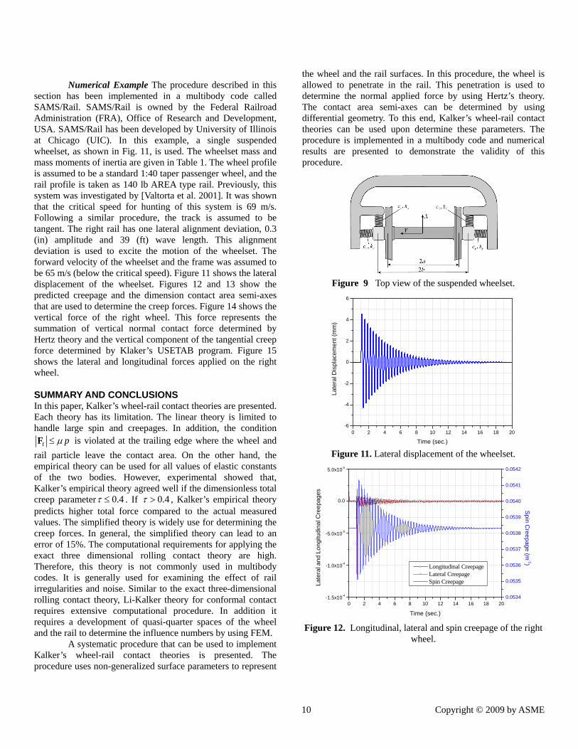
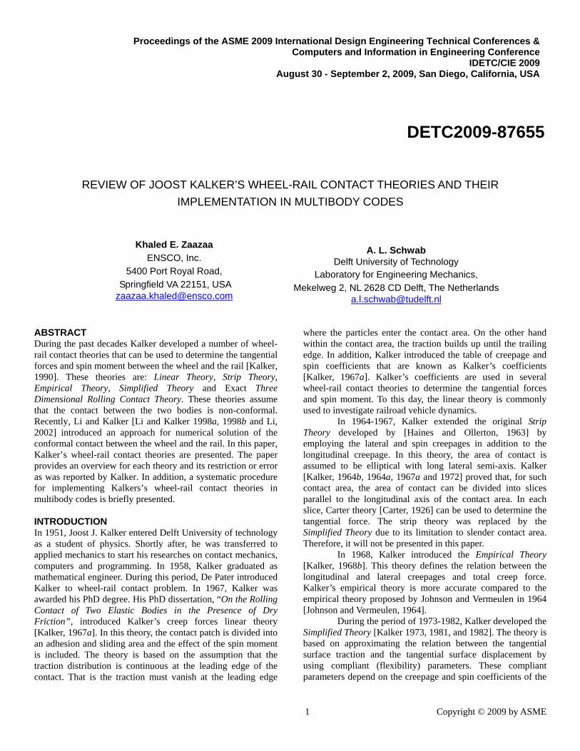
Numerical Example The procedure described in this

section has been implemented in a multibody code called SAMS/Rail. SAMS/Rail is owned by the Federal Railroad Administration (FRA), Office of Research and Development, USA. SAMS/Rail has been developed by University of Illinois at Chicago (UIC). In this example, a single suspended wheelset, as shown in Fig. 11, is used. The wheelset mass and mass moments of inertia are given in Table 1. The wheel profile is assumed to be a standard 1:40 taper passenger wheel, and the rail profile is taken as 140 lb AREA type rail. Previously, this system was investigated by [Valtorta et al. 2001]. It was shown that the critical speed for hunting of this system is 69 m/s. Following a similar procedure, the track is assumed to be tangent. The right rail has one lateral alignment deviation, 0.3 (in) amplitude and 39 (ft) wave length. This alignment deviation is used to excite the motion of the wheelset. The forward velocity of the wheelset and the frame was assumed to be 65 m/s (below the critical speed). Figure 11 shows the lateral displacement of the wheelset. Figures 12 and 13 show the predicted creepage and the dimension contact area semi-axes that are used to determine the creep forces. Figure 14 shows the vertical force of the right wheel. This force represents the summation of vertical normal contact force determined by Hertz theory and the vertical component of the tangential creep force determined by Klaker’s USETAB program. Figure 15 shows the lateral and longitudinal forces applied on the right wheel. SUMMARY AND CONCLUSIONS In this paper, Kalker’s wheel-rail contact theories are presented. Each theory has its limitation. The linear theory is limited to handle large spin and creepages. In addition, the condition

t pµ≤F is violated at the trailing edge where the wheel and rail particle leave the contact area. On the other hand, the empirical theory can be used for all values of elastic constants of the two bodies. However, experimental showed that, Kalker’s empirical theory agreed well if the dimensionless total creep parameter 0.4τ ≤ . If 0.4τ > , Kalker’s empirical theory predicts higher total force compared to the actual measured values. The simplified theory is widely use for determining the creep forces. In general, the simplified theory can lead to an error of 15%. The computational requirements for applying the exact three dimensional rolling contact theory are high. Therefore, this theory is not commonly used in multibody codes. It is generally used for examining the effect of rail irregularities and noise. Similar to the exact three-dimensional rolling contact theory, Li-Kalker theory for conformal contact requires extensive computational procedure. In addition it requires a development of quasi-quarter spaces of the wheel and the rail to determine the influence numbers by using FEM. A systematic procedure that can be used to implement Kalker’s wheel-rail contact theories is presented. The procedure uses non-generalized surface parameters to represent

the wheel and the rail surfaces. In this procedure, the wheel is allowed to penetrate in the rail. This penetration is used to determine the normal applied force by using Hertz’s theory. The contact area semi-axes can be determined by using differential geometry. To this end, Kalker’s wheel-rail contact theories can be used upon determine these parameters. The procedure is implemented in a multibody code and numerical results are presented to demonstrate the validity of this procedure.

Figure 9 Top view of the suspended wheelset.

0 2 4 6 8 10 12 14 16 18 20-6

-4

-2

0

2

4

6

Late

ral D

ispl

acem

ent (

mm

)

Time (sec.) Figure 11. Lateral displacement of the wheelset.

0 2 4 6 8 10 12 14 16 18 20-1.5x10-4

-1.0x10-4

-5.0x10-5

0.0

5.0x10-5

Longitudinal Creepage Lateral Creepage Spin Creepage

Time (sec.)

Late

ral a

nd L

ongi

tudi

nal C

reep

ages

0.0534

0.0535

0.0536

0.0537

0.0538

0.0539

0.0540

0.0541

0.0542

Spin C

reepage (m-1)

Figure 12. Longitudinal, lateral and spin creepage of the right

wheel.


Table 1 Suspended Wheelset Model

Variable Description Value

wm Wheelset mass 1568 kg w

xxI Inertia moment 656 kg·m2

wyyI Inertia moment 168 kg·m2

wzzI Inertia moment 656 kg·m2

W Applied vertical load per Wheel 49000 N

kxStiffness for longitudinal springs

1.35E+5 N/m

ky Stiffness for lateral springs 2.5E+5 N/m

cxDamping coefficient for longitudinal springs

0 N/m·s

cyDamping coefficient for lateral springs

0 N/m·s

2b Distance between longitudinal springs

1.8 m

2a Gage distance 1435 mm µ Wheel/rail friction 0.5

E Wheel and rail Modulus of Elasticity

2.1E+11 N/m2

ν Poisson’s Ratio 0.28

0 2 4 6 8 10 12 14 16 18 205.76

5.78

5.80

5.82

5.84

5.86

a b

Time (sec.)

a (m

m)

3.86

3.88

3.90

3.92

3.94

3.96

3.98

b (mm

)

Figure 13. Contact area semi-axes, a and b, of the right wheel.

0 2 4 6 8 10 12 14 16 18 2048.0

48.2

48.4

48.6

48.8

49.0

49.2

49.4

49.6

49.8

50.0

Ver

tical

For

ce (k

N)

Time (sec.)

Figure 14. Vertical contact force of the right wheel.

0 2 4 6 8 10 12 14 16 18 20-0.20

-0.15

-0.10

-0.05

0.00

0.05

0.10

0.15

0.20

0.25

Longitudinal Force Lateral Force

Time (sec.)

Long

itudi

nal F

orce

(kN

)

0.0

0.2

0.4

0.6

0.8

1.0

1.2

Lateral Force (KN)

Figure 15. Longitudinal and lateral forces of the right wheel.

ACKNOWLEDGMENTS The first author would like to acknowledge the support he received from the Federal Railroad Administration, Office of Research and Development. This support is highly appreciated.

REFERENCES 1. Carter, F. C., 1926, “On the Action of a Locomotive

Driving Wheel”, Proceedings of the Royal Society of London A, 112, p. 151-157.

2. Hertz, H., 1882, “Über die Berührung Fester Elastische Körper und Über die Harte“, Verhandlungen des Vereins zur Beförderung des Gewerbefleisses, Leipaig, Nov. 1882.

3. Haines, D. J., Ollerton, E., 1963, “Contact Stress Distribution on Elliptical Contact Surfaces Subjected to Radial and Tangential Forces”, Proceedings of the Institution of Mechanical Engineers, 177, p. 95-114.

4. Johnson, K. L., Vermeulen, P. J., 1964, “Contact of Non-Spherical Bodies Transmitting Tangential Forces“, Journal of Applied Mechanics, 25, p. 339-346.

5. Kalker, J. J., 1958, “The Transmission of Forces and Couples between two Elastically Similar Rolling Spheres”, manuscript, Report laboratory of applied mechanics, no 256.


6. Kalker, J. J., 1964a, “The Transmission of Force and Couple between Two Elastically Similar Rolling Spheres”, Proceedings Koninklijke Nederlandse Akademie van Wetenschappen, Amsterdam B 67(1964), p.135-177.

7. Kalker, J. J., 1964b, “A Strip Theory for Rolling with Slip and Spin”, Internal report 327, Department of Mechanical Engineering, Delft University of Technology.

8. Kalker, J. J., 1964c, “A Strip Theory for Rolling with Microslip and Spin”, Internal report 280, Delft University of Technology.

9. Kalker, J. J., 1966, “Rolling with Slip and Spin in the Presence of Dry Friction”, Wear 9, p. 20-38 .

10. Kalker, J. J., 1967a, “On the Rolling Contact of Two Elastic Bodies in the Presence of Dry Friction”, Doctoral Thesis, Delft.

11. Kalker, J. J., 1967b, “A Strip Theory for Rolling with Slip and Spin”, Koninklijke Nederlandse Akademie van Wetenschappen, Series B70, p. 10-62.

12. Kalker, J. J., 1968a, “Transient Rolling Contact Phenomena”, 12th Congress of Applied Mechanics, Stanford, CA, August 1968.

13. Kalker, J. J., 1968b, “The Tangential Force Transmitted by Two Elastic Bodies Rolling Over Each Other with Pure Creepage”, Wear,11,421-430.

14. Kalker, J. J., 1969, “The Approximation of the Creepage-force Law for Small Creepage and Arbitrary Spin”, Internal report Department of mechanical engineering.

15. Kalker, J. J., 1970, “Transient Phenomena in Two Elastic Cylinders Rolling Over Each Other with Dry Friction”, Journal of Applied Mechanics,37, p. 677-688

16. Kalker J. J., A. D. De Pater, 1971, “Survey of the Theory of Local Slip in the Elastic Contact Region with Dry Friction”, International Applied Mechanics 7(5) 472-483, Springer.

17. Kalker J. J., 1972, “On Elastic Line Contact”, Journal of Applied Mechanics 39, No 4, p.1125-1132.

18. Kalker, J. J., 1973, “Simplified Theory of Rolling Contact”, Progress Report, Delft University of Technology, Delft, The Netherlands, p. 1-10.

19. Kalker, J. J., 1977a, “A Survey of the Mechanics of Contact between Solid Bodies”, Zeitschrift für Angewandte Mathematik und Mechanik, 57, p. T3-T17.

20. Kalker, J. J., 1977b, “Variational Theory of Contact Elastostatics”, Journal of the Institute of Mathematics and its Applications 20, p. 199-219.

21. Kalker, J. J., 1979a, “The Computation of Three-Dimensional Rolling Contact with Dry Friction”, International Journal for numerical methods in engineering, Vol.14, p. 1293-1307, John Wiley and Sons, Ltd.

22. Kalker, J. J., 1979b, “Survey of Wheel-Rail Rolling Contact Theory, State-of-the-Art Paper”, IUTAM-IAVSD Symposium, Berlin, Vehicle System Dynamics 5(1979) p.317-358.

23. Kalker, J. J., 1980, "Review of Wheel-Rail Rolling Contact Theories", in The General Problem of Rolling Contact, L. Browne and N.T. Tsai (eds.), the 1989 ASME Winter Annual Meeting, Chicago, IL, AMD-Vol. 40, pp. 77-92.

24. Kalker, J. J., 1981, “A Fast Algorithm for the Simplified Theory of Rolling Contact, Report Faculty of Mathematics, TU Delft.

25. Kalker, J. J., 1982, "A Fast Algorithm for the Simplified Theory of Rolling Contact", Vehicle System Dynamics, Vol. 11, pp. 1-13.

26. Kalker, J. J., 1983, A Simplified Theory for Non-Hertzian Contact, Vehicle System Dynamics 12, p.43-45.

27. Kalker, J. J., 1986a, Railway Wheel and Automotive Tyre, Vehicle System Dynamics 5, Vol.15, p.255-269.

28. Kalker, J. J., 1986b, “The Principle of Virtual Work and Its Dual for Contact Problems”, Ingenieur-Archiv 56, p.453-467. Springer.

29. Kalker, J. J., 1986c, “Numerical Calculation of the Elastic Field in a Half-Space”, Communications of Applied Numerical Methods, 2, p.401-410.

30. Kalker, J. J., 1990, Three-Dimensional Elastic Bodies in Rolling Contact, Kluwer Academic Publishers, Dordrecht/Boston/London.

31. Kalker, J. J., 1991, Wheel-Rail Rolling Contact Theory, Wear 144, p.243-261.

32. Li, L. Z., Kalker J. J., 1998a, “The Computation of Wheel-Rail Conformal Contact”, Proceedings of the 4th World Conference on Computational Mechanics, 29 June-2 July, Buenos Aires, Argentina.

33. Li, L. Z., Kalker J. J., 1998b, “The Computation of Wheel-Rail Conformal Contact”, Computational Mechanics, New Trends and Applications, S. Idelsohm, E Onate and E Dvorkin (Eds), CIMME, Barcelona, Spain.

34. Li, L. Z., 2002, “Wheel-Rail Rolling Contact and Its Application to Wear Simulation”, PhD Thesis, Delft University Press, Delft, The Netherlands.

35. Shabana, A. A., Zaazaa, K. E., Sugiyama, H., 2008, Railroad Vehicle Dynamics: A Computational Approach, CRC Press, Taylor and Francis Group.

36. Shabana, A. A., Tobaa, M., Sugiyama, H. and Zaazaa, K.E., 2005, "On the Computer Formulations of the Wheel/Rail Contact ", Nonlinear Dynamics, Vol. 40, pp. 169–193.

37. Valtorta, D., Zaazaa, K. E., Shabana, A. A., Sany, J. R., 2001, “A Study of the Lateral Stability of Railroad Vehicles Using a Nonlinear Constrained Multibody Formulation”, Proceedings of 2001 ASME International Mechanical Engineering Congress and Exposition, New York, NY.

38. Zaazaa, K. E., 2003, "Elastic Force Model for Wheel/Rail Contact in Multibody Railroad Vehicle Systems", Ph.D. Thesis, Department of Mechanical Engineering, University of Illinois at Chicago, Chicago, IL.


REVIEW OF JOOST KALKER’S WHEEL-RAIL CONTACT THEORIES

Documents

Transcript of REVIEW OF JOOST KALKER’S WHEEL-RAIL CONTACT THEORIES