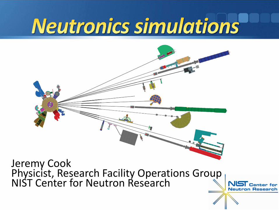
Jeremy CookPhysicist, Research Facility Operations GroupNIST Center for Neutron Research

Outline

Why do simulations?Available codes for neutron instrumentationAcceptance diagramsMonte Carlo simulations (emphasis on neutron guides and shielding)

Concepts and example for neutron guideExample of neutron guide profile optimizationExample of supermirror m optimizationSimple example for estimating neutron guide shieldingUse of neutron guide simulation results for MCNP shielding calculations

Why do simulations?

Modern computing technology and simulation codes offer a very cheap and powerful design and optimization tool

Can generate and store a wide variety of statistical quantities that would be very difficult or impossible to access in an experiment

Use for problems that are difficult to solve analytically or require excessive approximations

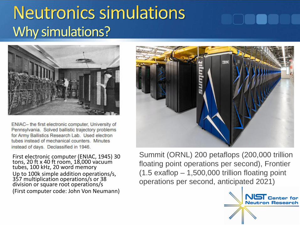
Why simulations?

First electronic computer (ENIAC, 1945) 30 tons, 20 ft x 40 ft room, 18,000 vacuum tubes, 100 kHz, 20 word memoryUp to 100k simple addition operations/s, 357 multiplication operations/s or 38 division or square root operations/s(First computer code: John Von Neumann)

Summit (ORNL) 200 petaflops (200,000 trillion floating point operations per second), Frontier (1.5 exaflop – 1,500,000 trillion floating point operations per second, anticipated 2021)

Recent developments for neutron scattering

New and upgraded neutron facilities pushed development of publicly-available, crowd-sourced simulation codes

Continual code maintenance/ development and debuggingComprehensive documentation and online tutorialsTested by many users!

Some private codes developed over many years but not publicly-available (e.g. mine!)

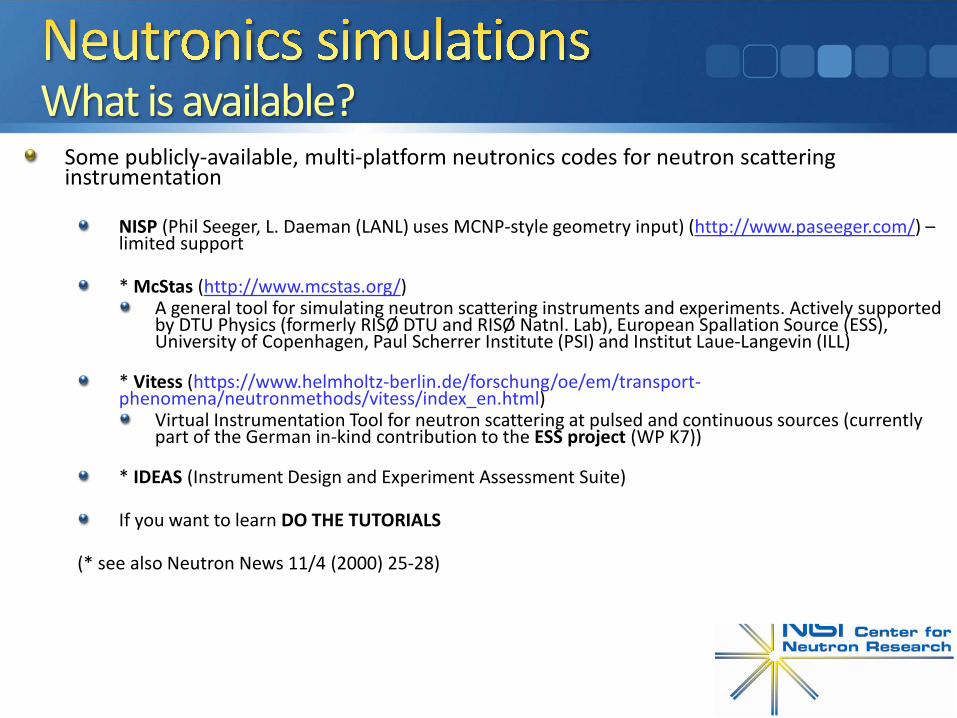
What is available?Some publicly-available, multi-platform neutronics codes for neutron scattering instrumentation

NISP (Phil Seeger, L. Daeman (LANL) uses MCNP-style geometry input) (http://www.paseeger.com/) –limited support

* McStas (http://www.mcstas.org/)A general tool for simulating neutron scattering instruments and experiments. Actively supported by DTU Physics (formerly RISØ DTU and RISØ Natnl. Lab), European Spallation Source (ESS), University of Copenhagen, Paul Scherrer Institute (PSI) and Institut Laue-Langevin (ILL)

* Vitess (https://www.helmholtz-berlin.de/forschung/oe/em/transport-phenomena/neutronmethods/vitess/index_en.html)

Virtual Instrumentation Tool for neutron scattering at pulsed and continuous sources (currently part of the German in-kind contribution to the ESS project (WP K7))

* IDEAS (Instrument Design and Experiment Assessment Suite)

If you want to learn DO THE TUTORIALS

(* see also Neutron News 11/4 (2000) 25-28)

Why simulations?

Other well-established (and tested) Monte Carlo particle transport codes e.g. GEANT4 (GEometryANdTracking), MCNP (Monte Carlo N-Particle)

GEANT4 (CERN) – Developed primarily for high-energy physicsMCNP (Los Alamos) – Developed originally for nuclear fission criticality and reactor physics

MCNP6– unified features of MCNPX and MCNP5 including high energy capabilities and particles of MCNPX)Good for nuclear reactor simulations/design (criticality problems), shielding design, etc.Neutron coherent scattering not handled by MCNP (cannot be used directly for guide simulations)

Acceptance diagrams (for neutron optics design)

Danger of “blind” Monte Carlo simulation is possibility of not recognizing erroneous results (e.g. due to erroneous input)

Acceptance diagrams valuable for understanding “allowed” regions of parameter space (usually space-angle) that are potentially transmitted by a guide

Restriction: Acceptance diagram is for a unique neutron energy/ wavelength (also 2-D)

Horizontal and vertical 2-D transmissions can be decoupled for rectangular cross-section guides (not the case for e.g. circular cross-sections)

Examples of acceptance diagrams for curved guides in “theory” presentation

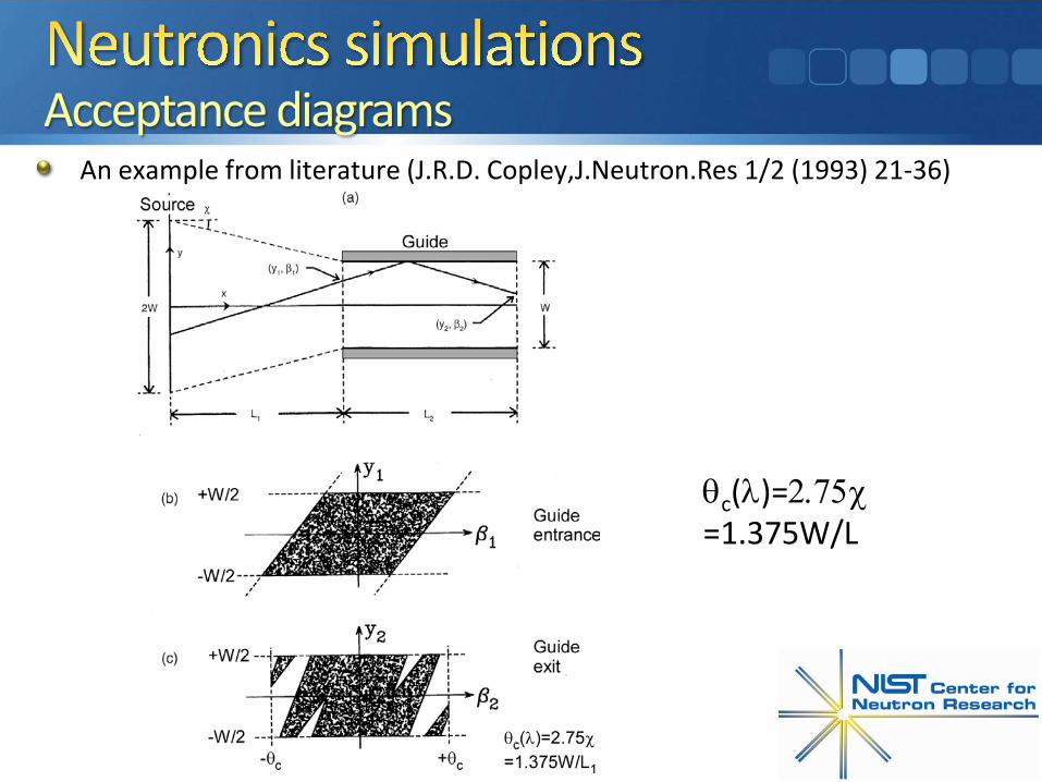
Acceptance diagramsAn example from literature (J.R.D. Copley, J.Neutron.Res 1/2 (1993) 21-36)

θc(λ)=2.75χ=1.375W/L

Acceptance diagramsAn example from literature (J.R.D. Copley, J.Neutron.Res 1/2 (1993) 21-36)

θc(λ)=2.75χ=1.375W/L

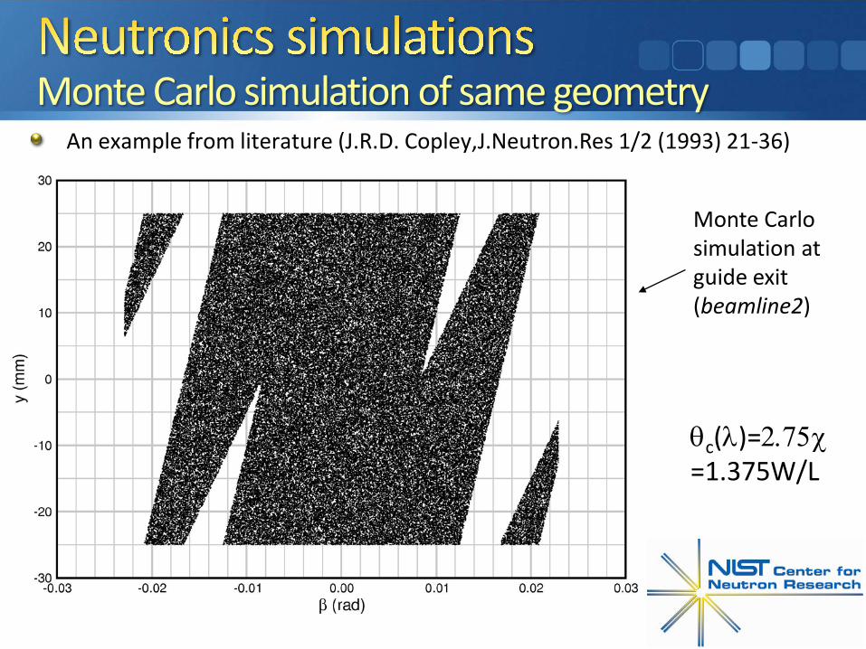
Monte Carlo simulation of same geometryAn example from literature (J.R.D. Copley, J.Neutron.Res 1/2 (1993) 21-36)

θc(λ)=2.75χ=1.375W/L

Monte Carlo simulation at guide exit (beamline2)

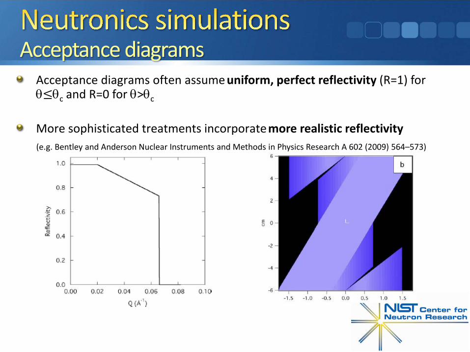
Acceptance diagramsAcceptance diagrams often assume uniform, perfect reflectivity (R=1) for θ≤θc and R=0 for θ>θc

More sophisticated treatments incorporate more realistic reflectivity(e.g. Bentley and Anderson Nuclear Instruments and Methods in Physics Research A 602 (2009) 564–573)

Monte Carlo simulations

Acceptance diagrams reveal allowed spatial-angular regions and give good insight

BUT… realistic reflectivities can render some of the allowed regions almost empty!

Latter phases of optical design usually performed with Monte Carlo simulations using realistic reflectivity models (both x,y dimensions and multi-wavelength are combined in one simulation)

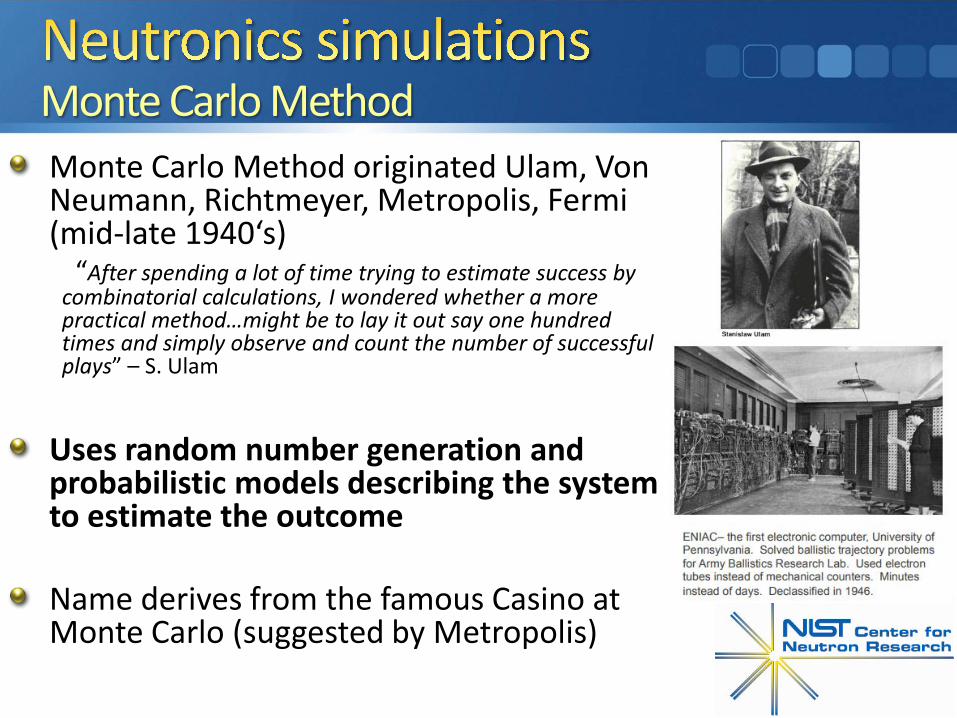
Monte Carlo MethodMonte Carlo Method originated Ulam, Von Neumann, Richtmeyer, Metropolis, Fermi (mid-late 1940‘s)

“After spending a lot of time trying to estimate success by combinatorial calculations, I wondered whether a more practical method…might be to lay it out say one hundred times and simply observe and count the number of successful plays” – S. Ulam

Uses random number generation and probabilistic models describing the system to estimate the outcome

Name derives from the famous Casino at Monte Carlo (suggested by Metropolis)

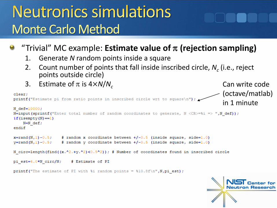
Monte Carlo Method“Trivial” MC example: Estimate value of π (rejection sampling)

1. Generate N random points inside a square2. Count number of points that fall inside inscribed circle, Nc (i.e., reject

points outside circle)3. Estimate of π is 4×N/Nc Can write code

(octave/matlab) in 1 minute

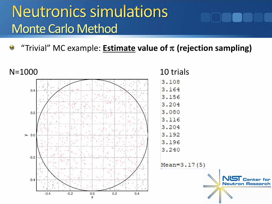
Monte Carlo Method“Trivial” MC example: Estimate value of π (rejection sampling)

N=1000 10 trials

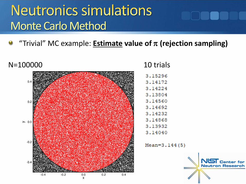
Monte Carlo Method“Trivial” MC example: Estimate value of π (rejection sampling)

N=100000 10 trials

GOLDEN RULE OF SIMULATIONS!

GARBAGE IN = GARBAGE OUT!

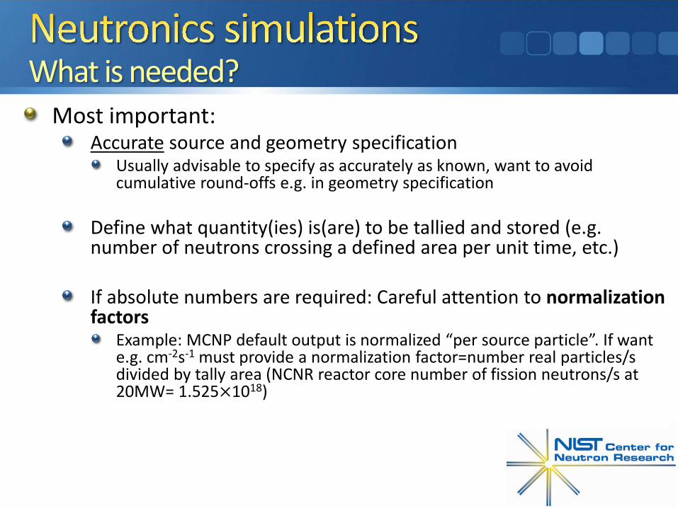
What is needed?Most important:

Accurate source and geometry specificationUsually advisable to specify as accurately as known, want to avoid cumulative round-offs e.g. in geometry specification

Define what quantity(ies) is(are) to be tallied and stored (e.g. number of neutrons crossing a defined area per unit time, etc.)

If absolute numbers are required: Careful attention to normalizationfactors

Example: MCNP default output is normalized “per source particle”. If want e.g. cm-2s-1 must provide a normalization factor=number real particles/s divided by tally area (NCNR reactor core number of fission neutrons/s at 20MW= 1.525×1018)

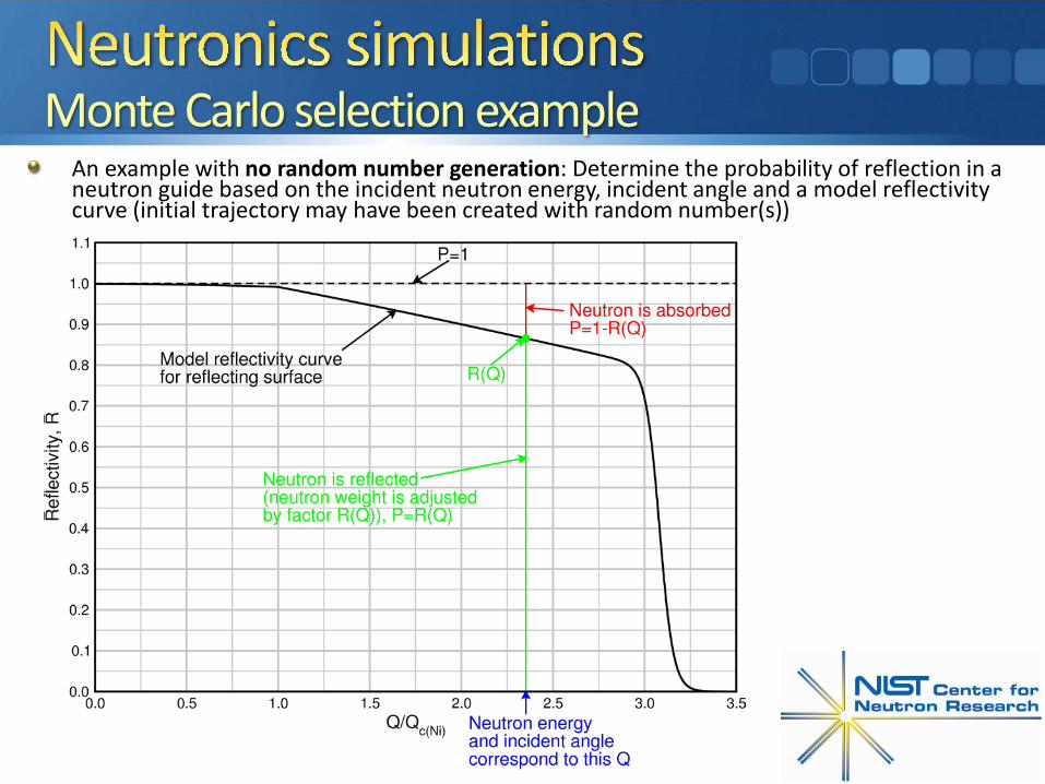
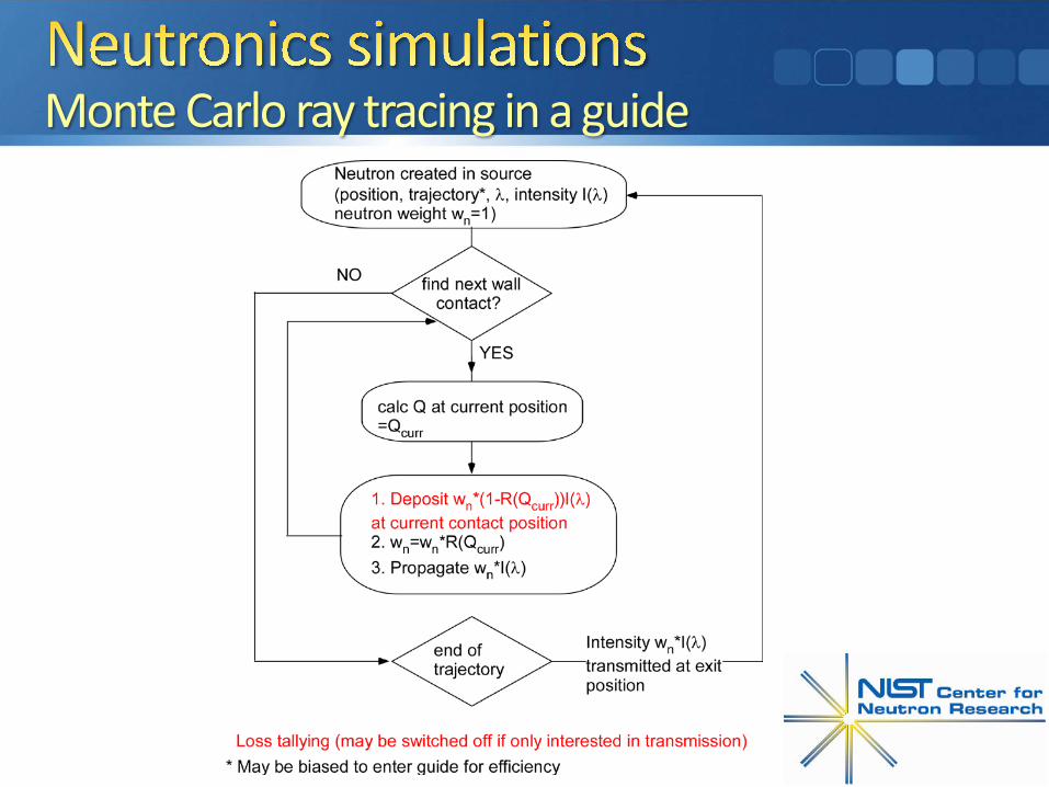
Monte Carlo selection exampleAn example with no random number generation: Determine the probability of reflection in a neutron guide based on the incident neutron energy, incident angle and a model reflectivity curve (initial trajectory may have been created with random number(s))

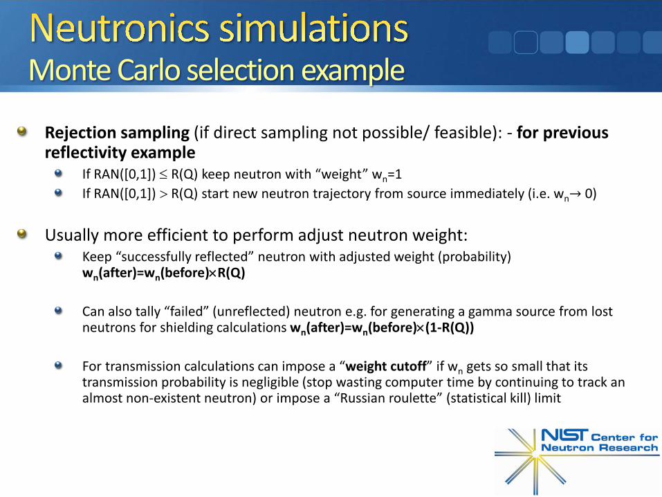
Monte Carlo selection example

Rejection sampling (if direct sampling not possible/ feasible): - for previous reflectivity example

If RAN([0,1]) ≤ R(Q) keep neutron with “weight” wn=1If RAN([0,1]) > R(Q) start new neutron trajectory from source immediately (i.e. wn→ 0)

Usually more efficient to perform adjust neutron weight:Keep “successfully reflected” neutron with adjusted weight (probability) wn(after)=wn(before)×R(Q)

Can also tally “failed” (unreflected) neutron e.g. for generating a gamma source from lost neutrons for shielding calculations wn(after)=wn(before)×(1-R(Q))

For transmission calculations can impose a “weight cutoff” if wn gets so small that its transmission probability is negligible (stop wasting computer time by continuing to track an almost non-existent neutron) or impose a “Russian roulette” (statistical kill) limit

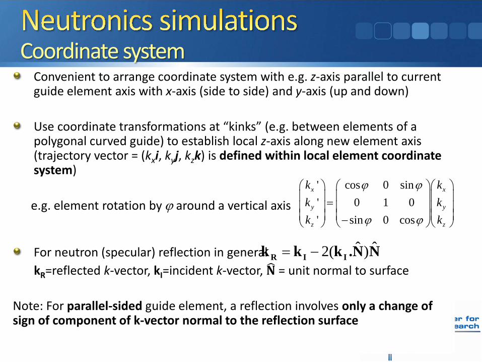
Coordinate systemConvenient to arrange coordinate system with e.g. z-axis parallel to current guide element axis with x-axis (side to side) and y-axis (up and down)

Use coordinate transformations at “kinks” (e.g. between elements of a polygonal curved guide) to establish local z-axis along new element axis (trajectory vector = (kxi, kyj, kzk) is defined within local element coordinate system)

e.g. element rotation by ϕ around a vertical axis' cos 0 sin' 0 1 0' sin 0 cos

x x

y y

z z

k kk kk k

ϕ ϕ

ϕ ϕ

= −

For neutron (specular) reflection in generalkR=reflected k-vector, kI=incident k-vector, 𝐍𝐍 = unit normal to surface

Note: For parallel-sided guide element, a reflection involves only a change of sign of component of k-vector normal to the reflection surface

ˆ ˆ2( )= −R I Ik k k .N N

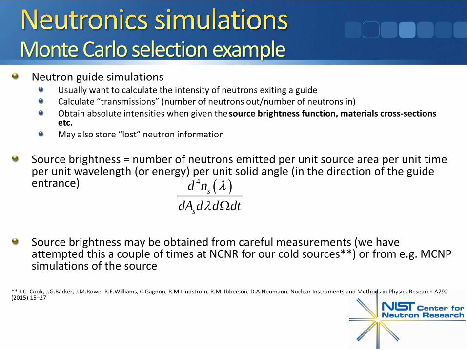
Monte Carlo selection exampleNeutron guide simulations

Usually want to calculate the intensity of neutrons exiting a guideCalculate “transmissions” (number of neutrons out/number of neutrons in)Obtain absolute intensities when given the source brightness function, materials cross-sections etc.May also store “lost” neutron information

Source brightness = number of neutrons emitted per unit source area per unit time per unit wavelength (or energy) per unit solid angle (in the direction of the guide entrance)

Source brightness may be obtained from careful measurements (we have attempted this a couple of times at NCNR for our cold sources**) or from e.g. MCNP simulations of the source

** J.C. Cook, J.G.Barker, J.M.Rowe, R.E.Williams, C.Gagnon, R.M.Lindstrom, R.M. Ibberson, D.A.Neumann, Nuclear Instruments and Methods in Physics Research A792 (2015) 15–27

( )4s

s

d ndA d d dt

λλ Ω

Monte Carlo ray tracing in a guide

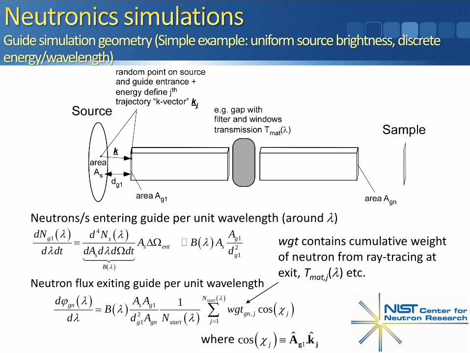
Guide simulation geometry (Simple example: uniform source brightness, discrete energy/wavelength)

Neutrons/s entering guide per unit wavelength (around λ)( ) ( )

( )

( )4

1 121

g gss ent s

s g

B

dN Ad NA B A

d dt dA d d dt dλ

λ λλ

λ λ= ∆Ω

Ω

( ) ( ) ( ) ( )( )

1,

121

cos1 startNgn s g

jg gn stan

rtg j j

d A AN

td A

gd

wBλϕ λ

λλ

χλ =

= ∑

Neutron flux exiting guide per unit wavelength

.

( ) 1ˆ ˆcos .jχ ≡ g jA kwhere

wgt contains cumulative weight of neutron from ray-tracing at exit, Tmat,j(λ) etc.

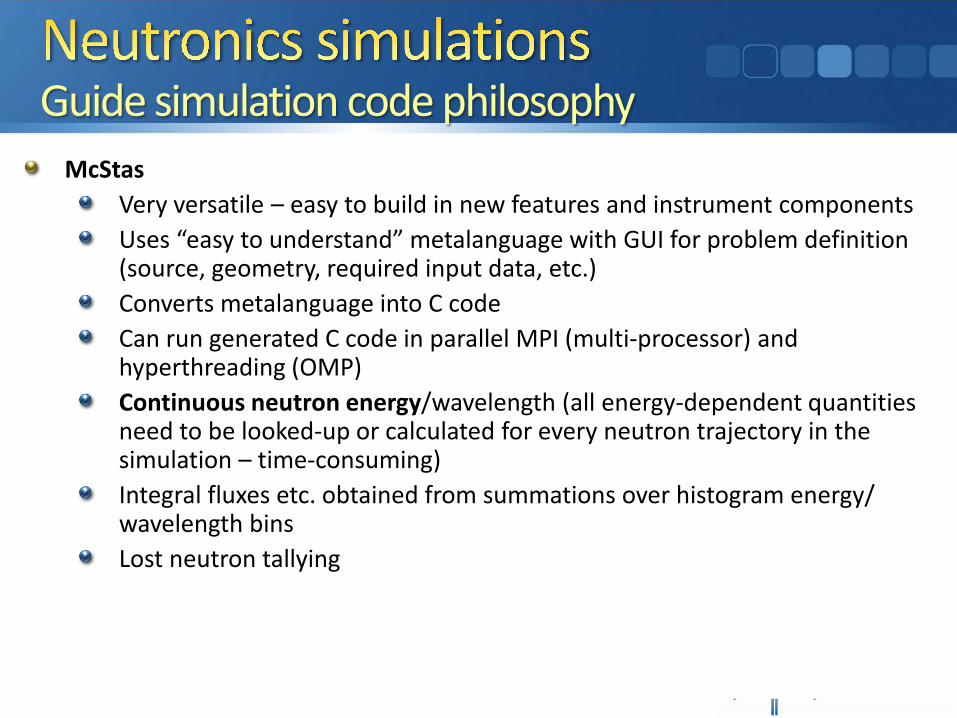
Guide simulation code philosophyMcStas

Very versatile – easy to build in new features and instrument componentsUses “easy to understand” metalanguage with GUI for problem definition (source, geometry, required input data, etc.)Converts metalanguage into C codeCan run generated C code in parallel MPI (multi-processor) and hyperthreading (OMP)Continuous neutron energy/wavelength (all energy-dependent quantities need to be looked-up or calculated for every neutron trajectory in the simulation – time-consuming)Integral fluxes etc. obtained from summations over histogram energy/ wavelength binsLost neutron tallying

Guide simulation code philosophyMy code (beamline2 – Fortran 90-2003)

More rigid format input (less versatile for additions of new components, options) (considering more versatile input)Discrete neutron energy/ wavelength (by design) – all energy-dependent quantities can be calculated outside of main calculation loops (very efficient)Integral fluxes etc. obtained by integration (only need to be careful of step size)Discrete energy approach produces statistically-identical results to McStas for guides much fasterLost neutron tallying (turned off when not needed)

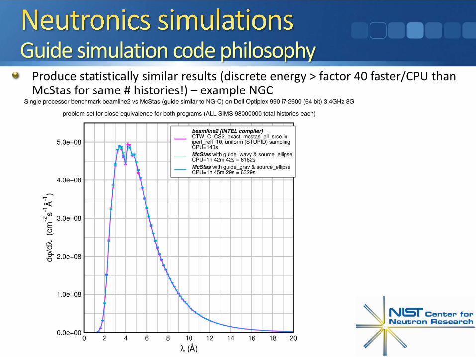
Guide simulation code philosophyProduce statistically similar results (discrete energy > factor 40 faster/CPU than McStas for same # histories!) – example NGC

Guide simulation: Guide profile optimizationExample: Re-optimization of focusing guide for HFBS

Start with an approximation (original HFBS tapered guide) divided into a number of elements

Optimize profile with “blanket” supermirror coating of high m (e.g. all m=4)

Choose optimization criterion (e.g. neutrons/s on a defined area), wavelength/energy range, range of guide elements to adjust …

Iteratively adjust entrance/exit dimensions of defined elements with constraint e.g. wex,i=went,i+1 or hex,i=hent,i+1

Alternate entrance-to-exit, exit-to-entrance each time finding (local) optimum of criterion for each element (stop/ adjust dimension step length if going away from optimum)

Repeat trying to converge on global optimum

Guide simulation: Guide profile optimization(For beamline2) perl script engine:1. Runs simulation code2. Analyses and plots results3. Updates input to “best yet” and adjusts step size according to results4. Repeats until convergence criterion

McStas has similar utility guide_bot (MATLAB script, Mads Bertelsen)

guide_bot modified by Leland Harriger (NCNR) to optimize bi-elliptical replacement for NG-5 whilst accounting for monochromator performance

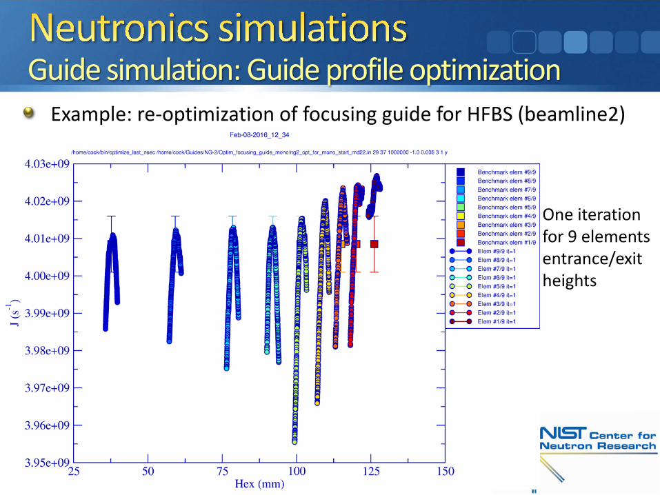
Guide simulation: Guide profile optimizationExample: re-optimization of focusing guide for HFBS (beamline2)

One iteration for 9 elementsentrance/exit heights

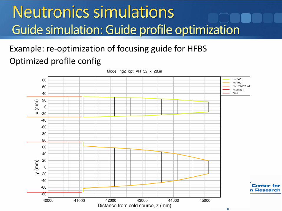
Guide simulation: Guide profile optimizationExample: re-optimization of focusing guide for HFBSStarting profile configExample: re-optimization of focusing guide for HFBSOptimized profile config

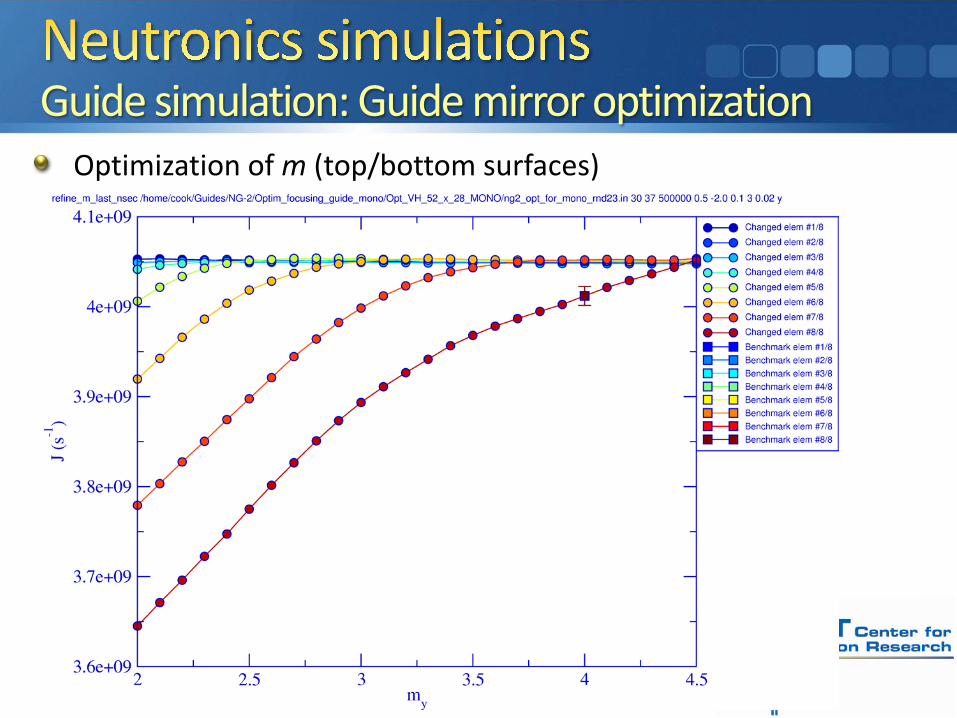
Guide simulation: Guide mirror optimizationOptimization of m (top/bottom surfaces)

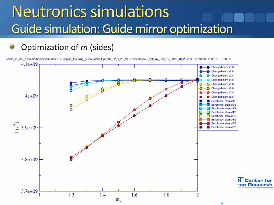
Guide simulation: Guide mirror optimizationOptimization of m (sides)

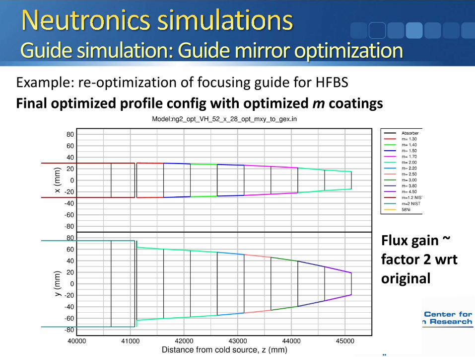
Guide simulation: Guide mirror optimizationExample: re-optimization of focusing guide for HFBSFinal optimized profile config with optimized m coatings

Flux gain ~ factor 2 wrtoriginal

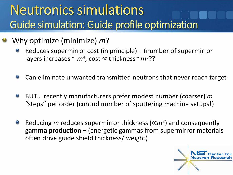
Guide simulation: Guide profile optimizationWhy optimize (minimize) m?

Reduces supermirror cost (in principle) – (number of supermirror layers increases ~ m4, cost ∝ thickness~ m3??

Can eliminate unwanted transmitted neutrons that never reach target

BUT… recently manufacturers prefer modest number (coarser) m“steps” per order (control number of sputtering machine setups!)

Reducing m reduces supermirror thickness (∝m3) and consequently gamma production – (energetic gammas from supermirror materials often drive guide shield thickness/ weight)

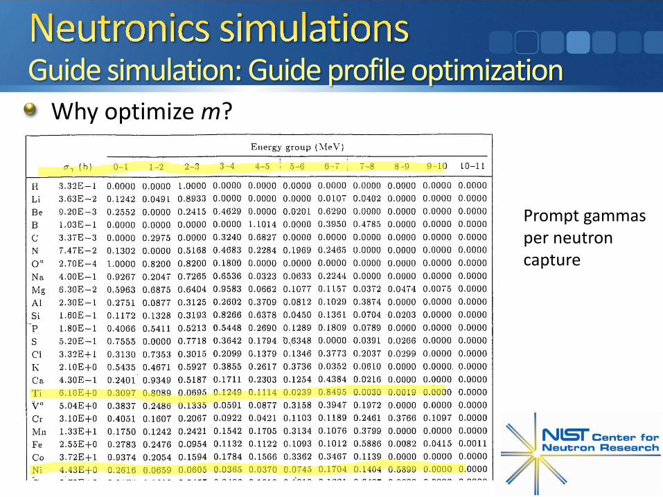
Guide simulation: Guide profile optimizationWhy optimize m?

Prompt gammas per neutron capture

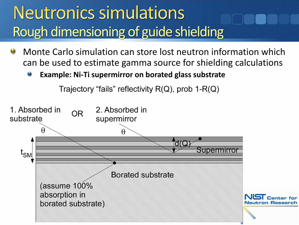
Rough dimensioning of guide shieldingMonte Carlo simulation can store lost neutron information which can be used to estimate gamma source for shielding calculations

Example: Ni-Ti supermirror on borated glass substrate

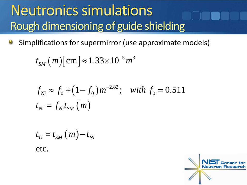
Rough dimensioning of guide shieldingSimplifications for supermirror (use approximate models)

( )[ ]

( )( )

( )

5 3

2.830 0 0

cm 1.33 10

1 ; 0.511

etc.

SM

Ni

Ni Ni SM

Ti SM Ni

t m m

f f f m with f

t f t m

t t m t

−

−

≈ ×

≈ + − =

=

= −

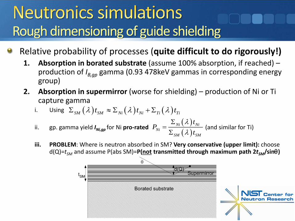
Rough dimensioning of guide shieldingRelative probability of processes (quite difficult to do rigorously!)

1. Absorption in borated substrate (assume 100% absorption, if reached) –production of IB,gp gamma (0.93 478keV gammas in corresponding energy group)

2. Absorption in supermirror (worse for shielding) – production of Ni or Ticapture gamma

i. Using

ii. gp. gamma yield INi,gp for Ni pro-rated (and similar for Ti)

iii. PROBLEM: Where is neutron absorbed in SM? Very conservative (upper limit): choose d(Q)=tSM and assume P(abs SM)=P(not transmitted through maximum path 2tSM/sinθ)

( ) ( ) ( )SM SM Ni Ni Ti Tit t tλ λ λΣ ≈ Σ +Σ

( )( )

Ni NiNi

SM SM

tP

tλλ

Σ=Σ

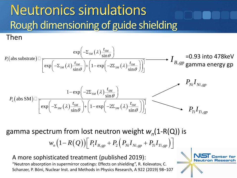
Rough dimensioning of guide shieldingThen

gamma spectrum from lost neutron weight wn(1-R(Q)) is

A more sophisticated treatment (published 2019):“Neutron absorption in supermirror coatings: Effects on shielding”, R. Kolevatov, C. Schanzer, P. Böni, Nuclear Inst. and Methods in Physics Research, A 922 (2019) 98–107

( )( )

( ) ( )2

1 exp 2sinabs SM

exp 1 exp 2sin sin

SMSM

SM SMSM SM

t

Pt t

λθ

λ λθ θ

− − Σ

−Σ + − − Σ

,Ni Ni gpP I

,Ti Ti gpP I

( )( ) ( )1 , 2 , ,1n B gp Ni Ni gp Ti Ti gpw R Q PI P P I P I − + +

( )( )

( ) ( )1

expsinabs substrate

exp 1 exp 2sin sin

SMSM

SM SMSM SM

t

Pt t

λθ

λ λθ θ

−Σ

−Σ + − − Σ

=0.93 into 478keV gamma energy gp,B gpI

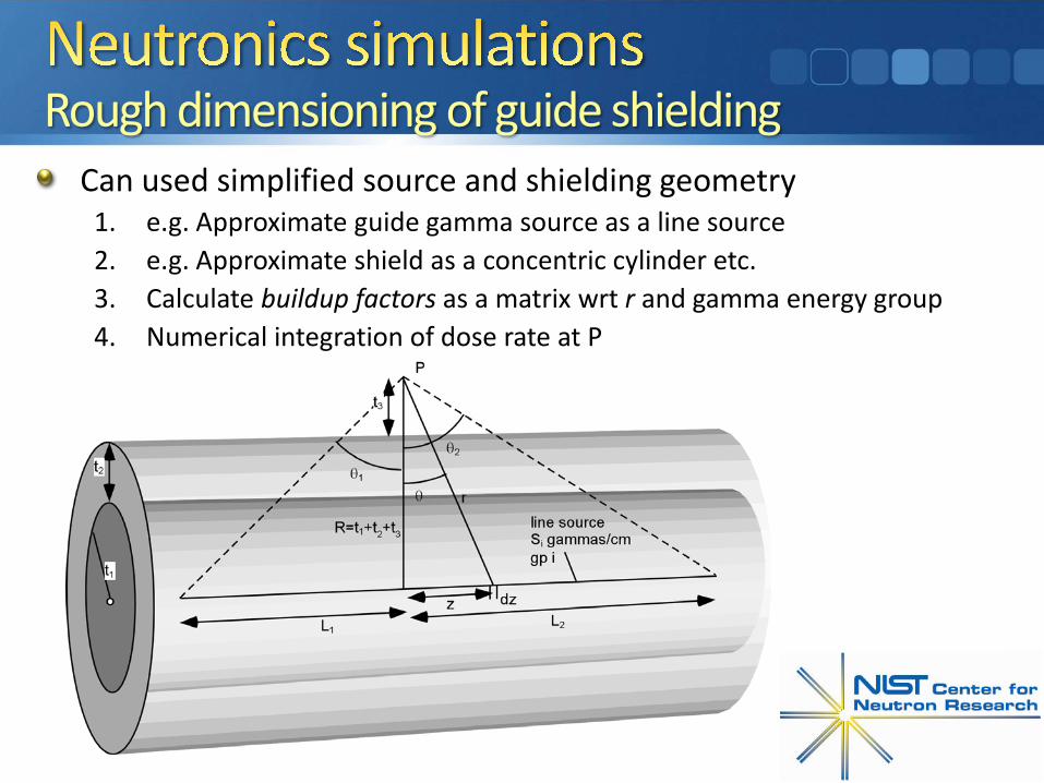
Rough dimensioning of guide shieldingCan used simplified source and shielding geometry

1. e.g. Approximate guide gamma source as a line source2. e.g. Approximate shield as a concentric cylinder etc.3. Calculate buildup factors as a matrix wrt r and gamma energy group4. Numerical integration of dose rate at P

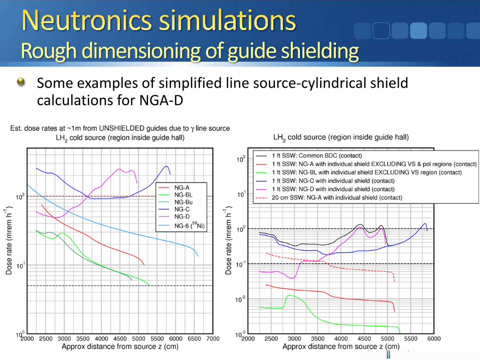
Rough dimensioning of guide shieldingSome examples of simplified line source-cylindrical shield calculations for NGA-D

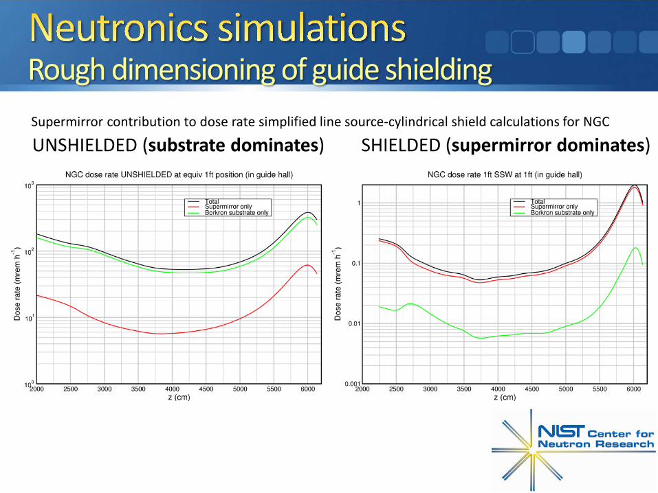
Rough dimensioning of guide shieldingSupermirror contribution to dose rate simplified line source-cylindrical shield calculations for NGC

UNSHIELDED (substrate dominates) SHIELDED (supermirror dominates)

Rough dimensioning of guide shielding

Other in-guide sources (e.g. V or double-V polarizer) may require enhanced shielding

e.g. VSANS double-V~ 0.3mm thick Si at 0.75° × 2 ≈ 4.6cm Si traversed by beamUsually requires more than the standard 30cm SSW on neutron beams in the NCNR guide hall

MCNP?MCNP cannot do coherent scattering required for neutron transport in guides

Can approximate the neutron beam at the exit of a guide with required spectrum and energy-dependent divergence (remember θc∝λ)

Some limitations on MCNP user-defined source: e.g. cannot decouple horizontal and vertical divergence differences ⇒ approximate by mean polar angle

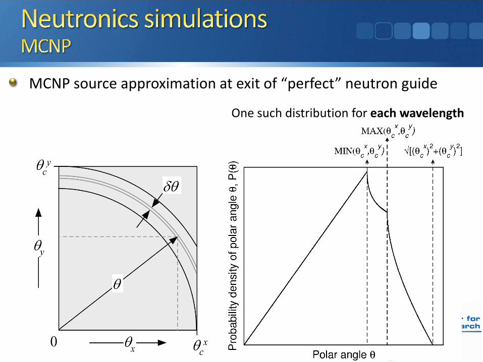
MCNP source approximation at exit of “perfect” neutron guide

One such distribution for each wavelength

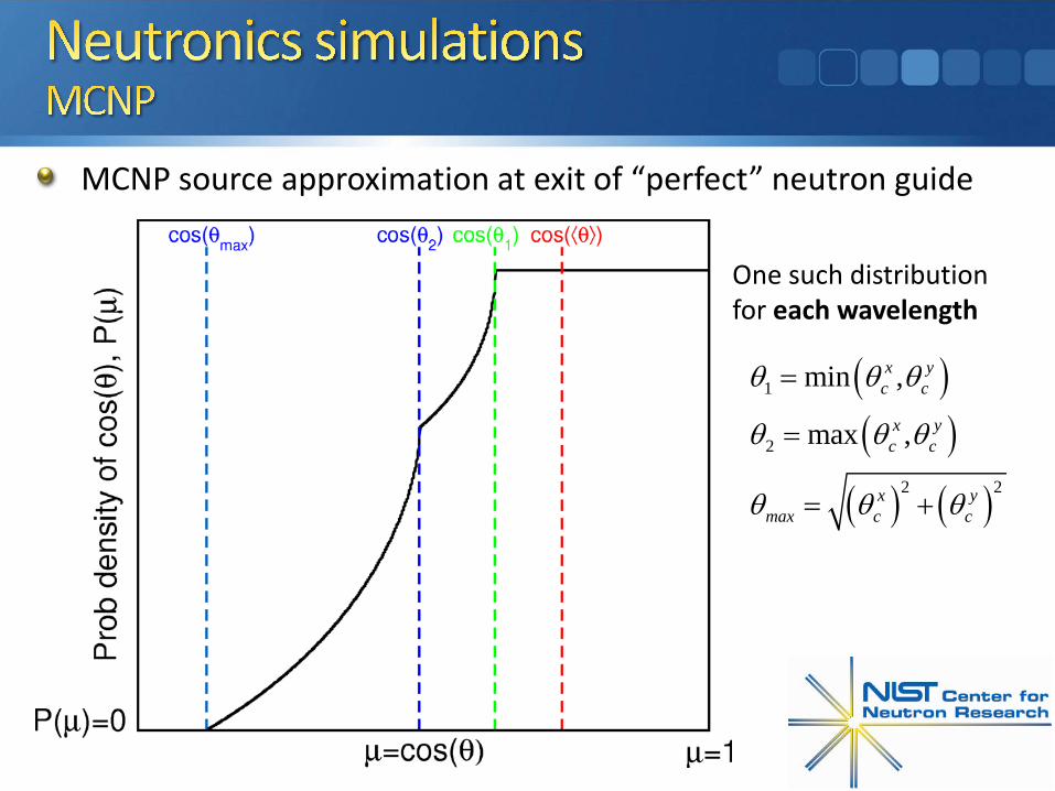
MCNP source approximation at exit of “perfect” neutron guide

One such distribution for each wavelength

( )( )( ) ( )

1

2

2 2

min ,

max ,

x yc c

x yc c

x ymax c c

θ θ θ

θ θ θ

θ θ θ

=

=

= +

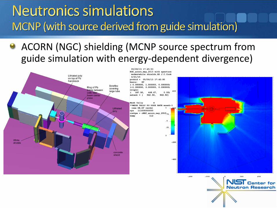
ACORN (NGC) shielding (MCNP source spectrum from guide simulation with energy-dependent divergence)

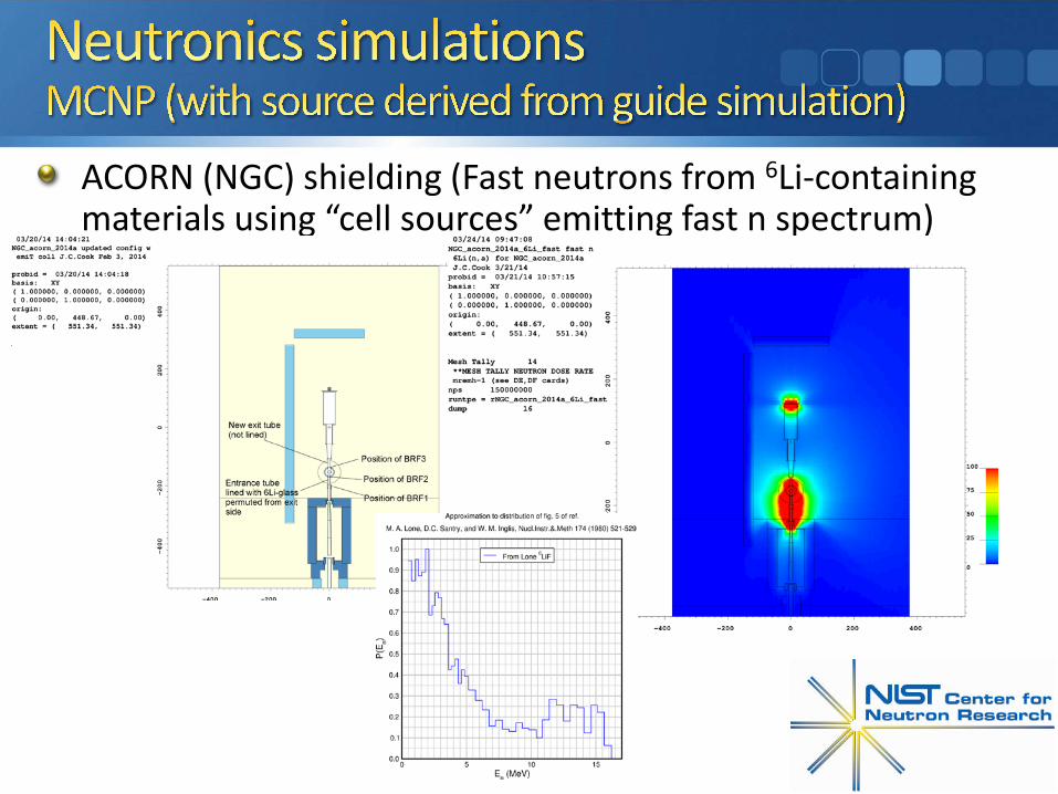
ACORN (NGC) shielding (Fast neutrons from 6Li-containing materials using “cell sources” emitting fast n spectrum)

END😴😴