Research Article

Saleem Obaidat* and Rizwan Butt

A new implicit symmetric method of sixthalgebraic order with vanished phase-lagand its first derivative for solvingSchrödinger's equation

https://doi.org/10.1515/math-2021-0009received July 23, 2020; accepted January 9, 2021

Abstract: In this article, we have developed an implicit symmetric four-step method of sixth algebraic orderwith vanished phase-lag and its first derivative. The error and stability analysis of this method are investi-gated, and its efficiency is tested by solving efficiently the one-dimensional time-independent Schrödinger’sequation. The method performance is compared with other methods in the literature. It is found that for thisproblem the new method performs better than the compared methods.

Keywords: phase-lag, stability analysis, implicit symmetric method, Schrödinger equation, truncation error

MSC 2020: 65D15, 65D20, 34A50

1 Introduction

The numerical solution of second-order initial-value problems with periodical and/or oscillatory solutionsas:

″( ) = ( ( )) ( ) = ′( ) = ′q x f x q x q x q q x q, , and ,0 0 0 0 (1.1)

has attracted the attention of many authors in the last decades [1–25]. The aim of these studies was the pro-duction of efficient, fast, and reliable algorithms for solving this model. These algorithms are of two maintypes, namely, algorithms with constant coefficients as given in Jain et al. [9] and Steifel and Bettis [10],and other ones with variable coefficients depending on the problem frequency as presented in [18–31]. Inpractice, equation (1.1) has been used to present mathematical models in several disciplines, such as,chemistry, quantum chemistry, physics, quantum mechanics, etc. The one-dimensional time-independentSchrödinger equation:

″( ) =

( + )

+ ( ) − ( )y φ l lφ

V φ τ y φ1 .22 (1.2)

is an example. Usually, the solution of equation (1.2) is studied under two boundary conditions, the first oneis ( ) =y 0 0, and a second condition corresponds to large values of φ, which can be adopted due to somephysical considerations. Here, τ2 is a real number denoting the energy, l is an integer representing theangular momentum, and V is the potential function which satisfies ( ) →V φ 0 as → ∞φ .

* Corresponding author: Saleem Obaidat, Department of Mathematics, College of Science, King Saud University, Kingdom ofSaudi Arabia, e-mail: saleem@ksu.edu.saRizwan Butt: Department of Mathematics, College of Science, King Saud University, Kingdom of Saudi Arabia

Open Mathematics 2021; 19: 225–237

Open Access. © 2021 Saleem Obaidat and Rizwan Butt, published by De Gruyter. This work is licensed under the CreativeCommons Attribution 4.0 International License.

In the literature, a lot of research works have been done in developing numerical methods of differenttypes for solving equation (1.2). Explicit multistep phase-fitted methods are developed by Lambert andWatson in [32], Anastassi and Simos in [23], Simos and Williams in [33], Alolyan and Simos [34], Simos in[35–37], and Obaidat and Mesloub in [38]. An implicit multistep phase-fitted methods is constructed in [39].Predictor corrector methods are designed by Panopoulos et al. in [40], Stasinos and Simos in [27], andSimos in [28]. Exponentially fitted multistep methods are provided by Simos in [26], Zhang et al. in [31], andG. Avdelas et al. in [41]. Exponentially and trigonometrically fitted multistep methods are developed byKonguetsof and Simos designed in kong, and Simos constructed in [29]. Runge-Kutta methods are pre-sented by Dormand and Prince in [42], Yang et al. in [43], and Yang et al. in [44]. Runge-Kutta-Nyströmmethods are constructed by Dormand et al. in [45]. Methods of Obrechkof-type are derived by Krishnaiahin [14], Achar in [16], Van Daele and Berghe in [17], and Jain in [9].

The aim of this paper is to develop a new efficient numerical method of the second type for solvingthe one-dimensional time-independent Schrödinger’s equation. Our approach is based on the symmetricmulti-step methods introduced by Quinlan and Tremaine [3], as well as the recent methodology for devel-oping numerical methods, for approximating the periodical solutions of certain initial-value problems,which requires nullifying the method phase-lag and some of its successive derivatives. Following thismethodology, we will develop an implicit four-step symmetric numerical method with vanished phase-lag and its first derivative for solving equation (1.2). The rest of this article is organized as the following. InSection 2, we present the basic theory from the literature. In Section 3, we present the method development.In Section 4, we provide the error and the stability analysis of the new method. In Section 5, we present theapplication of the method and the numerical results. Finally, in Section 6, we give some conclusions.

2 Preliminaries

A numerical solution of a mathematical model of type (1.1) can be obtained using multi-step methods as:

∑ ∑= ( )

=

+

=

+ +a q h b f x q, ,

i

m

i n ii

m

i n i n i0

2

0(2.1)

by dividing the interval of definition of the initial value problem under consideration into m subintervalseach of length h, using a finite set of equally spaced points { }

=xi i

k0, where = ∣ − ∣

+h x xi i1 , for = … −i m0, 1, , 1.

If m is an even integer and =−

a aj m j and =−

b bj m j for = …j 0, 1, , m2 , then such method is called symmetric

multi-step numerical method.Usually, an operator � is associated with the linear multi-step method (2.1); it is given by:

� ∑ ∑( ) = ( + ) − ″( + )

= =

x a ψ x jh h b ψ x jh ,j

m

jj

m

j0

2

0(2.2)

where ψ is a two times continuously differentiable function.Without loss of generality, as scaling equation (2.1) by a nonzero constant will not affect the forth-

coming results, we may take =a 1m ; so that equation (2.1) takes the form of a m2 -step symmetric method as:

∑ ∑+ ( + ) = + ( + )

=

+ −

=

+ −a q a q q h b f b f f ,n

k

m

k n k n k nk

m

k n k n k01

20

1(2.3)

where = ( )± ± ±

f f x q,n k n k n k .

Definition 2.1. [23] The multi-step method (2.1) is said to have an algebraic order r whenever the values of

the corresponding operator � vanish at any function ( ) = ∑=

+p x c x ,jr

jj

01 for any real numbers = …c j, 0, 1, ,j

+r 1.

226 Saleem Obaidat and Rizwan Butt

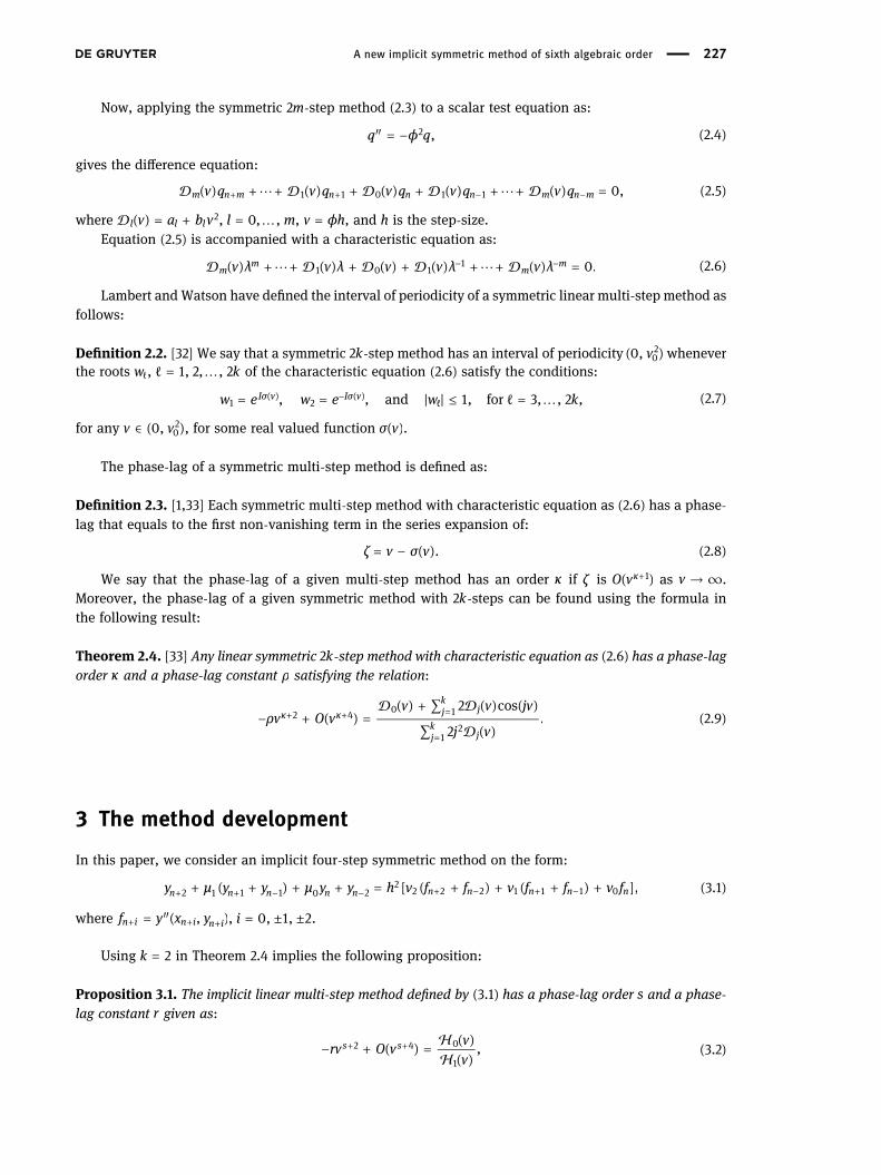
Now, applying the symmetric m2 -step method (2.3) to a scalar test equation as:

″ = −q ϕ q,2 (2.4)

gives the difference equation:

� � � � �( ) + ⋯+ ( ) + ( ) + ( ) + ⋯+ ( ) =+ + − −

v q v q v q v q v q 0,m n m n n n m n m1 1 0 1 1 (2.5)

where � ( ) = +v a b vl l l2, = …l m0, , , =v ϕh, and h is the step-size.

Equation (2.5) is accompanied with a characteristic equation as:

� � � � �( ) + ⋯+ ( ) + ( ) + ( ) + ⋯+ ( ) =− −v λ v λ v v λ v λ 0.m

mm

m1 0 1

1 (2.6)

Lambert andWatson have defined the interval of periodicity of a symmetric linear multi-step method asfollows:

Definition 2.2. [32] We say that a symmetric k2 -step method has an interval of periodicity ( )v0, 02 whenever

the rootsℓ

w , ℓ = … k1, 2, , 2 of the characteristic equation (2.6) satisfy the conditions:

= = ∣ ∣ ≤ ℓ = …( ) − ( )

ℓw e w e w k, , and 1, for 3, , 2 ,Iσ v Iσ v

1 2 (2.7)

for any ∈ ( )v v0, ,02 for some real valued function ( )σ v .

The phase-lag of a symmetric multi-step method is defined as:

Definition 2.3. [1,33] Each symmetric multi-step method with characteristic equation as (2.6) has a phase-lag that equals to the first non-vanishing term in the series expansion of:

= − ( )ζ v σ v . (2.8)

We say that the phase-lag of a given multi-step method has an order κ if ζ is ( )+O vκ 1 as → ∞v .

Moreover, the phase-lag of a given symmetric method with k2 -steps can be found using the formula inthe following result:

Theorem 2.4. [33] Any linear symmetric k2 -step method with characteristic equation as (2.6) has a phase-lagorder κ and a phase-lag constant ρ satisfying the relation:

� �

�− + ( ) =

( ) + ∑ ( ) ( )

∑ ( )

+ +=

=

ρv O vv v jv

j v

2 cos

2.κ κ j

kj

jk

j

2 4 0 1

12

(2.9)

3 The method development

In this paper, we consider an implicit four-step symmetric method on the form:

+ ( + ) + + = [ ( + ) + ( + ) + ]+ + − − + − + −

y μ y y μ y y h ν f f ν f f ν f ,n n n n n n n n n n2 1 1 1 0 22

2 2 2 1 1 1 0 (3.1)

where = ″( )+ + +

f y x y,n i n i n i , = ± ±i 0, 1, 2.

Using =k 2 in Theorem 2.4 implies the following proposition:

Proposition 3.1. The implicit linear multi-step method defined by (3.1) has a phase-lag order s and a phase-lag constant r given as:

�

�− + ( ) =

( )

( )

+ +rv O v vv

,s s2 4 0

1(3.2)

A new implicit symmetric method of sixth algebraic order 227

where

� � � � �( ) = ( ) ( ) + ( ) ( ) + ( ) ( ) = ( ) + ( )H v v v v v v H v v v2 cos 2 2 cos , 8 2 ,0 2 1 0 1 2 1

and � ( ) = +v μ ν vi i i2, =i 0, 1, 2.

In the method (3.1), we choose the parameters μ0, μ1, and μ2 so that this method is consistent andhas the highest algebraic order, while the coefficients ν0, ν1, and ν2 are considered as free parameters. Thus,

we take =μ 12 , =

−μ115

16 , and =

−μ01

8 . Then, using these values in equation (3.1) yields the following numer-ical method:

− ( + ) − + = [ ( + ) + ( + ) + ]+ + − − + − + −

y y y y y h ν f f ν f f ν f1516

18

.n n n n n n n n2 1 1 0 22

2 2 2 1 1 1 0 0 (3.3)

Hence, in view of (3.2), the method (3.3) has a phase-lag given by:

( ) =

( )

( )

PL vϕ vϕ v

,1

2(3.4)

where

( ) ≔ − + + − + + ( + )ϕ v v ν v v ν v v ν18

2 cos 1516

4 cos 1 ,12

02

12

2

and

( ) ≔ − + + ( + )ϕ v v ν v ν2 1516

8 1 .22

12

2

The following conditions are imposed on the new method:

( ) =

′( ) =

+ + =

PL vPL v

ν ν ν

0,0,

16 32 32 49,0 1 2

(3.5)

which will be used to find the values of the free parameters in equation (3.3).Thus, solving the system (3.5) for the parameters ν0, ν1, and ν2, we obtain:

=

( )

( )

=

− ( )

( )

=

− ( )

( )

νψ vψ v

νψ v

ψ vν

ψ vψ v

, ,2

,01

01

2

02

3

0(3.6)

where

( ) = ( ) + ( ) − ( ) − ( ) ( ) + ( ) − ( )

+ ( ) ( ) + ( ) ( ) + ( ) − ( ) ( ) − ( ) ( )

( ) = + ( ) − ( ) − ( ) ( ) + ( ) + ( )

− ( ) ( ) − ( ) − ( ) + ( ) ( )

( ) = − − ( ) + ( ) + ( ) − ( ) ( ) − ( ) + ( )

+ ( ) ( ) + ( ) − ( ) ( )

( ) = (− ( ) + ( ) ( ) + ( ) − ( ) ( ))

ψ v v v v v v v v vv v v v v v v v v v v v v v

ψ v v v v v v v vv v v v v v v v v v

ψ v v v v v v v v v vv v v v v v v v

ψ v v v v v v v v

4 cos 60 cos 4 cos 2 124 cos cos 2 64 cos 2 2 sin2 cos 2 sin 49 cos 2 sin 4 sin 2 4 cos sin 2 98 cos sin 2 ,

2 30 cos 34 cos 2 30 cos cos 2 32 cos 2 15 sin15 cos 2 sin 30 sin 2 49 sin 2 30 cos sin 2 ,

4 56 cos 60 cos 64 cos 2 64 cos cos 2 32 sin 49 sin32 cos 2 sin 64 sin 2 64 cos sin 2 ,

16 sin cos 2 sin 2 sin 2 2 cos sin 2 .

12 2

3 3

22

3

32 3

03

As it appears in (3.6), the expressions of ν0, ν1, and ν2 involve the frequency =v ϕh. Moreover, thenumerators and denominators in these expressions approach zero as →v 0. To avoid the arising hugeround-off errors due to this situation, the following series expansions of these expressions are used:

228 Saleem Obaidat and Rizwan Butt

= + − − − − − ⋯

= − + − − − − ⋯

= + + + + + + ⋯

ν v v v v v

ν v v v v v

ν v v v v v

18731920

35911520

1059358400

8209212889600

2178023498161664000

391187996323328000

,

467480

35917280

40073628800

8747958003200

77381373621248000

1074114483454976000

,

2713840

35969120

2166758060800

1088693832012800

71531172988969984000

395032717933819904000

.

02 4 6 8 10

12 4 6 8 10

22 4 6 8 10

(3.7)

Figures 1–3 represent the behaviors of the parameters ν0, ν1, and ν2, respectively.

Figure 1: Behavior of ν0.

Figure 2: Behavior of ν1.

Figure 3: Behavior of ν2.

A new implicit symmetric method of sixth algebraic order 229

4 The method error and stability analysis

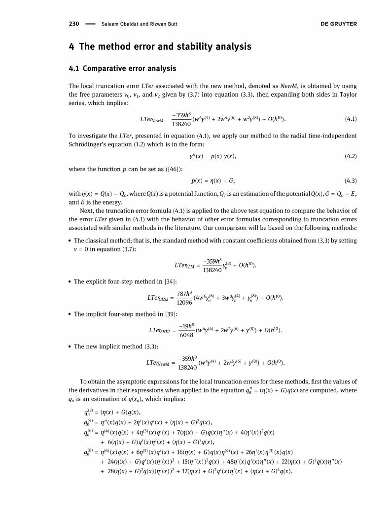
4.1 Comparative error analysis

The local truncation error LTer associated with the new method, denoted as NewM, is obtained by usingthe free parameters ν0, ν1, and ν2 given by (3.7) into equation (3.3), then expanding both sides in Taylorseries, which implies:

=

−

( + + ) + ( )( ) ( ) ( )LTer h w y w y w y O h359

1382402 .NewM

86 4 4 6 2 8 10 (4.1)

To investigate the LTer, presented in equation (4.1), we apply our method to the radial time-independentSchrödinger’s equation (1.2) which is in the form:

″( ) = ( ) ( )y x p x y x , (4.2)

where the function p can be set as ([46]):( ) = ( ) +p x η x G, (4.3)

with ( ) = ( ) −η x Q x Qc, where ( )Q x is a potential function,Qc is an estimation of the potential ( )Q x , = −G Q Ec ,and E is the energy.

Next, the truncation error formula (4.1) is applied to the above test equation to compare the behavior ofthe error LTer given in (4.1) with the behavior of other error formulas corresponding to truncation errorsassociated with similar methods in the literature. Our comparison will be based on the following methods:

• The classical method; that is, the standardmethodwith constant coefficients obtained from (3.3) by setting=v 0 in equation (3.7):

=

−

+ ( )( )LTer h y O h359

138240.CLM n

88 10

• The explicit four-step method in [34]:

= ( + + ) + ( )( ) ( ) ( )LTer h w y w y y O h787

120964 3 .OLS2 n n n

86 6 8 4 8 10

• The implicit four-step method in [39]:

=

−

( + + ) + ( )( ) ( ) ( )LTer h w y w y y O h19

60482 .SHK2

84 4 2 6 8 10

• The new implicit method (3.3):

=

−

( + + ) + ( )( ) ( ) ( )LTer h w y w y y O h359

1382402 .NewM

84 4 2 6 8 10

To obtain the asymptotic expressions for the local truncation errors for these methods, first the values ofthe derivatives in their expressions when applied to the equation ″ = ( ( ) + ) ( )q η x G q xn are computed, whereqn is an estimation of ( )q xn , which implies:

= ( ( ) + ) ( )

= ″( ) ( ) + ′( ) ′( ) + ( ( ) + ) ( )

= ( ) ( ) + ( ) ′( ) + ( ( ) + ) ( ) ″( ) + ( ′( )) ( )

+ ( ( ) + ) ′( ) ′( ) + ( ( ) + ) ( )

= ( ) ( ) + ( ) ′( ) + ( ( ) + ) ( ) ( ) + ′( ) ( ) ( )

+ ( ( ) + ) ′( )( ′( )) + ( ″( )) ( ) + ′( ) ′( ) ″( ) + ( ( ) + ) ( ) ″( )

+ ( ( ) + ) ( )( ′( )) + ( ( ) + ) ′( ) ′( ) + ( ( ) + ) ( )

( )

( )

( ) ( ) ( )

( ) ( ) ( ) ( ) ( )

q η x G q xq η x q x η x q x η x G q xq η x q x η x q x η x G q x η x η x q x

η x G q x η x η x G q xq η x q x η x q x η x G q x η x η x η x q x

η x G q x η x η x q x η x q x η x η x G q x η xη x G q x η x η x G q x η x η x G q x

,2 ,4 7 4

6 ,6 16 26

24 15 48 2228 12 .

n

n

n

n

2

4 2

6 4 3 2

3

8 6 5 4 3

3 2 2

2 2 2 4

230 Saleem Obaidat and Rizwan Butt

Then, using the expressions of ( )qnj , = …j 2, 4, , 8 in the above error formulas of the above methods gives

the following asymptotic expansions for the LTer corresponding to each one of these numerical methods:

• The classical scheme (3.1), i.e., the numerical method with constant coefficients obtained by setting =v 0in equation (3.3):

=

−

( ) + ⋯ + ( )LTEr h q x G O h359138240

.CLM8 4 10

• The explicit four-step method in [34]:

= ( ) ″( ) + ′( ) ′( ) + ( ) ( ) + ⋯ + ( )LTEr h q x g x g x q x y x g x G O h8657

6048787

10087872016

.OSII8 2 2 10

• The method derived in [39]:

= − [( ( ′( )) ( ) + ′( ) ′( ) + ″( ) ( )) + ⋯] + ( )LTEr h g x q x g x q x g x q x G O h196048

28 2 9 .SHK28

2 2 10

• The new method given by equation (3.3):

= − [( ( )( ′( )) + ′( ) ′( ) + ( ) ″( )) + ⋯] + ( )LTEr h q x g x g x q x q x g x G O h359138240

28 2 9 .NewM8

2 2 10

We see from these equations that the expressions of these truncation errors involve powers of the expres-sion = −G V Ec . Therefore, we should consider the following cases:

Case 1. ≈G 0, i.e., when the values of the energy E and the potentialVc are close to each other. In this case,in comparing the expressions of the truncation errors in these methods, we need to check only the termsfree of G. Hence, it follows that all these methods are of comparable accuracy, as these terms are identicalin all these methods.

Case 2. ≪G 0 or ≫G 0, i.e., when the values of the energy E and the potentialVc are significantly differentfrom each other, that is, ∣ ∣G is large.

In this case, we see from the above asymptotic error expressions that for the classical method the asymp-totic error increases as the third power ofG, whereas it increases as the first power ofG for the othermethods.But, for the newmethod,G has the lowest coefficients among all the above methods. Thus, for the numericalsolution of the radial time-independent Schrödinger’s equation with large values of ∣ ∣G , it seems to be that,among these numerical techniques, the new derived one is the most efficient.

4.2 Stability analysis

To study the stability analysis of the new numerical method, we substitute the values of the parameters ν0,ν1, and ν2 given in equation (3.6) in the method (3.3), then apply the resulting scheme to the test equation

″ = −y θ y2 , which produces a difference equation associated with the following characteristic equation:

� � � � �+ + + + =λ λ λ λ 0,24

13

02

1 2

where � = + ν s12 22, � = +

− ν s115

16 12, � = +

− ν s01

8 02, and =s θh. Here, the frequency ϕ of the derived

method (3.3) is different than the frequency of the test equation θ. The stability region of the constructedmethod is presented in Figure 4, in which the shaded parts represent the region on which the method isstable. Hence, in view of this region it follows that the periodicity interval of this new numerical scheme is(0, 10.5177).

A new implicit symmetric method of sixth algebraic order 231

5 Numerical results and discussion

To examine the efficiency of the constructed method, we apply it to solve the radial time-independentSchrödinger equation:

″( ) =

( + )

+ ( ) − ( )p φ l lφ

V φ γ p φ1 ,22 (5.1)

accompanied with two conditions:

( ) =p 0 0, (5.2)

and another boundary condition will be adapted to certain physical considerations for some large valueof φ. Here, γ2 in equation (5.1) is a constant that stands for the energy, l is the angular momentum, and Vrepresents the potential which satisfies ( ) →V φ 0 whenever → ∞φ .

The new constructed method involves non-constant parameters, as they depend on the frequency ofthe studied model. Thus, in order to apply this method to solve equation (5.1), first of all we need to specifya value for the frequency ϕ. Therefore, we consider (5.1) with =l 0, and choose ϕ as:

= ∣ ( ) − ∣ϕ V φ E , (5.3)

where ≔E γ2 is the energy, and use the Woods-Saxon potential:

( ) =

( + )

−

+

V φ uγ u u

501

501

,2 (5.4)

where =

−

u eφ

γ7and =a 0.6. The behavior of ( )V φ is shown in Figure 5.

In Woods-Saxon potential, the frequency ϕ is not a function in φ, instead it is approximated byestimating the potential ( )V φ at the certain potential critical points [46].

For the numerical tests, we take ϕ as follows (see [46])

=

+ ∈ [ ]

∈ [ ]

ϕE φ

E φ50 , 0, 6.5 ,

, 6.5, 15 .(5.5)

Figure 4: New method stability region.

232 Saleem Obaidat and Rizwan Butt

For large values of φ, the potential ( )V φ in equation (5.1) vanishes faster than ( + )l lφ

12 . Thus, equation (5.1)

reduces to:

″ + −

( + )

=p γ l lφ

1 0,22 (5.6)

which has the two linearly independent solutions, ( )γφj γxl and ( )γφN γφl , where ( )j γφl and ( )N γφl are theBessel and Neumann spherical functions, respectively. Hence, as → ∞φ , equation (5.1) has a solution inasymptotic form as:

≈ ( ) − ( ) ≈ − + ( ) −p Aγφj γx BγφN γφ AC γφ lπ δ γφ lπsin

2tan cos

2,l l l

where δl represents the phase shift that can be determined by the formula:

=

( ) ( ) − ( ) ( )

( ) ( ) − ( ) ( )

+ +

+ +

δy φ S φ y φ S φy φ C φ y φ C φ

arctan ,li i i i

i i i i

1 1

1 1(5.7)

where+

φi 1 andφi are two successivepoints in the asymptotic region,with ( ) = ( )S φ γφj γφl and ( ) = ( )C φ γφN γφl .

Now, given the energy E, we will employ the new method (3.3) to solve the resonance problem; that is,to estimate the phase shift δl which has exact value that equals to π

2 . But, first we need to determine the start

values pi for = …i 0, 1, , 3. Thus, in view of the condition (5.2) we get =p 00 , and the remaining other valuescan be computed using Runge-Kutta-Nyström methods (see [45] and [42]). Starting with these values,we will estimate the value of δl at the point

+φi 1 using the following numerical schemes:

• The explicit 8-step eighth order linear symmetric method with constant coefficients given in [3]; denote itby ( )QT 8 .

• The explicit 10-step tenth order linear symmetric method with constant coefficients developed in [3];denote it as ( )QT 10 .

• The explicit 12-step twelfth order linear symmetric method with constant coefficients developed in [3];denote it by ( )QT 12 .

• The explicit fourth order 4-step linear symmetric method with vanished phase-lag and its first derivativegiven in [35]; denote it as SIMI.

• The explicit fourth order 4-step linear symmetric method with vanished phase-lag and its first and secondderivatives constructed in [36]; denote it by SIM.

• The explicit fourth order 4-step symmetric method with vanished phase-lag and its first and secondderivatives given in [37]; denote it as SIMN.

Figure 5: Behavior of Woods-Saxon potential.

A new implicit symmetric method of sixth algebraic order 233

• The eighth order two-stage two-step linear symmetric method with vanished phase-lag and its first, second,third, and fourth derivatives obtained in [47]; denote it by S St2 .

• The eighth order three stage two-step linear symmetricmethodwith vanished phase-lag and its first, second,third, and fourth derivatives developed in [48]; denote it as S St3 .

• The three-stage fifth order two-derivative Runge-Kutta method, developed in [43]; denote it by Y D2 .• The fourth order three derivative Runge-Kutta method with vanished phase-lag and its first derivativeproduced in [44]; denote it as Y D3 .

• The implicit sixth order 4-step linear symmetric method with vanished phase-lag and its first derivativein [39]; denote it by SHIM.

• The explicit fourth order 4-step linear symmetric method with vanished phase-lag and its first derivativedeveloped in [38]; denote it by EFSM.

• The implicit fourth order 4-step symmetric classical method (with constant coefficients) given in Section 2.3;denote it as CLM.

• The new developed implicit sixth-order 4-step linear symmetric method with vanished phase-lag and itsfirst derivative given in equation (3.3) developed in Section 2; denote it by NewM.

The efficiency of the new developed method is tested against these methods via computing the CPUtime (in seconds) required to get different accuracy digits in estimating the value of δl using the two energyvalues, =E 341.4958741 and =E 989.7019162 . Then, the absolute error = ∣ ( )∣MER ERlog :

= −ER π δ2

,l comp,

is graphed versus the required consumed CPU time (in seconds) corresponding to the energies E1 and E2,as shown in Figures 6 and 7, respectively.

6 Conclusions

The results in Figures 6 and 7 show that the efficiency of the new developed implicit method (NewM) insolving Schrödinger equation with different energy values is confirmed, as it gives the highest accuracyamong the other compared methods in less CPU time.

0 1 2 3 4 5 6 7ln(CPU time) in seconds

0

2

4

6

8

10

12

14

Accu

racy

dig

its

Resonance problem: E1=341.495874

NewMCLMSHIMEFSMSIMISIMIISIMSIMNQT8QT10QT12S2StS3StY2DY3D

Figure 6: Methods efficiency using E 341.4958741 = .

234 Saleem Obaidat and Rizwan Butt

Acknowledgments: The authors extend their appreciation to the Deanship of Scientific Research at KingSaud University for funding this work through research group no. (RG-1441-338).

Conflict of interest: Authors state no conflict of interest.

References

[1] R. M. Thomas, Phase properties of high order almost P-stable formulae, BIT 24 (1984), 225–238.[2] A. D. Raptis and A. C. Allison, Exponential-fitting methods for the numerical solution of the Schrödinger equation, Comput.

Phys. Commun. 14 (1978), 1–5.[3] D. G. Quinlan and S. Tremaine, Symmetric multistep methods for the numerical integration of planetary orbits, Astron. J.

100 (1990), no. 5, 1694–1700.[4] J. Coleman and L. Ixaru, P-stability and exponential-fitting methods for y f x y″ ,= ( ), IMA J. Numer. Anal. 16 (1996),

179–199.[5] G. D. Quinlan, Resonances and instabilities in symmetric multi-step methods, arXiv:astro-ph/9901136, (1999).[6] Z. Wang, P-stable linear symmetric multistep methods for periodic initial-value problems, Comput. Phys. Commun. 171

(2005), 162–174.[7] S. D. Capper, J. R. Cash, and D. R. Moore, Lobatto-Obrechkoff formulae for 2nd order two-point boundary value problems,

J. Numer. Anal. Ind. Appl. Math. 1 (2006), no. 1, 13–25.[8] H. Van de Vyver, Phase-fitted and amplification-fitted two-step hybrid methods for y f x y″ ,= ( ), J. Comput. Appl. Math. 209

(2007), no. 1, 33–53.[9] M. K. Jain, R. K. Jain, and U. A. Krishnaiah, Obrechkoff methods for periodic initial value problems of second order

differential equations, J. Math. Phys. Sci. 15 (1981), no. 3, 239–250.[10] E. Stiefel and D. G. Bettis, Stabilization of Cowell’s method, Numer. Math. 13 (1969), 154–175.[11] M. M. Chawla and P. S. Rao, A Noumerov-type method with minimal phase-lag for the integration of second order periodic

initial value problems. II. Explicit method, J. Comput. Appl. Math. 15 (1986), no. 3, 329–337.[12] G. Dahlquist, On accuracy and unconditional stability of linear multistep methods for second order differential equations,

BIT 18 (1978), no. 2, 133–136.[13] J. M. Franco, An explicit hybrid method of Numerov type for second-order periodic initial-value problems, J. Comput. Appl.

Math. 59 (1995), no. 1, 79–90.[14] U. A. Krishnaiah, P-stable Obrechkoffmethods with minimal phase-lag for periodic initial value problems, Math. Comp. 49

(1987), no. 180, 553–559.[15] G. Saldanha and S. D. Achar, Symmetric multistep methods with zero phase-lag for periodic initial value problems of

second order differential equations, Appl. Math. Comput. 175 (2006), no. 1, 401–412.

0 1 2 3 4 5 6 7 8 9

ln(CPU time) in seconds

0

5

10

15

Accu

racy

dig

its

Resonance problem: E2=989.701916

NewMCLMSHIMEFSMSIMISIMIISIMSIMNQT-8QT-10QT-12S2StS3StY2DY3D

Figure 7: Methods efficiency using E 989.7019162 = .

A new implicit symmetric method of sixth algebraic order 235

[16] S. D. Achar, Symmetric multistep Obrechkoff methods with zero phase-lag for periodic initial value problems of secondorder differential equations, Appl. Math. Comput. 218 (2011), no. 5, 2237–2248.

[17] M. Van Daele and G. V. Berghe, P-stable exponentially-fitted Obrechkoff methods of arbitrary order for second-orderdifferential equations, Numer. Algorithms 46 (2007), no. 4, 333–350.

[18] J. Vigo-Aguiar and H. Ramos, On the choice of the frequency in trigonometrically-fitted methods for periodic problems,J. Comput. Appl. Math. 277 (2015), 94–105.

[19] J. Vigo-Aguiar and H. Ramos, A strategy for selecting the frequency in trigonometrically-fitted methods based onthe minimization of the local truncation errors and the total energy error, J. Math. Chem. 52 (2014), 1050–1058.

[20] H. Ramos and J. Vigo-Aguiar, A trigonometrically-fitted method with two frequencies, one for the solution and another onefor the derivative, Comput. Phys. Commun. 185 (2014), no. 4, 1230–1236.

[21] H. Ramos and J. Vigo-Aguiar, Variable-stepsize Chebyshev-type methods for the integration of second-order I.V.P.’s,J. Comput. Appl. Math. 204 (2007), 102–113.

[22] H. Ramos and J. Vigo-Aguiar, A variable-step Numerov method for the numerical solution of the Schrödinger equation,J. Math. Chem. 37 (2005), 255–262.

[23] Z. A. Anastassi and T. E. Simos, A parametric symmetric linear four-step method for the efficient integration ofthe Schrödinger equation and related oscillatory problems, J. Comput. Appl. Math. 236 (2012), no. 16, 3880–3889.

[24] I. Alolyan, Z. A. Anastassi, and T. E. Simos, A new family of symmetric linear four-step methods for the efficient integrationof the Schrödinger equation and related oscillatory problems, Appl. Math. Comput. 218 (2012), no. 9, 5370–5382.

[25] Z. A. Anastassi, A new symmetric linear eight-step method with fifth trigonometric order for the efficient integration ofthe Schrödinger equation, Appl. Math. Lett. 24 (2011), no. 8, 1468–1472.

[26] T. E. Simos, Exponentially-fitted multiderivative methods for the numerical solution of the Schrödinger equation, J. Math.Chem. 36 (2004), 13–27.

[27] P. I. Stasinos and T. E. Simos, Symmetric embedded predictor-predictor-corrector (EPPCM)methods with vanished phase-lag and its derivatives for second order problems, AIP Conf. Proc. 1906 (2017), no. 1, 200023, DOI: https://doi.org/10.1063/1.5012499.

[28] T. E. Simos, Predictor-corrector phase-fitted methods for Y F X Y″ ,= ( ) and an application to the Schrödinger equation,Int. J. Quantum Chem. 53 (1995), no. 5, 473–483.

[29] T. E. Simos, Exponentially and trigonometrically fitted methods for the solution of the Schrödinger equation, Acta Appl.Math. 110 (2010), no. 3, 1331–1352.

[30] A. Konguetsof and T. E. Simos, An exponentially-fitted and trigonometrically-fitted method for the numerical solution ofperiodic initial-value problems, Comput. Math. Appl. 45 (2003), no. 1–3, 547–554.

[31] Y. Zhang, X. You, and Y. Fang, Exponentially fitted multi-derivative linear methods for the resonant state of the Schrödingerequation, J. Math. Chem. 55 (2017), 223–237.

[32] J. D. Lambert and I. A. Watson, Symmetric multistep methods for periodic initial value problems, IMA J. Appl. Math. 18(1976), no. 2, 189–202.

[33] T. E. Simos and P. S. Williams, A finite-difference method for the numerical solution of the Schrdinger equation, J. Comput.Appl. Math. 79 (1997), 189–205.

[34] I. Alolyan and T. A. Simos, Family of explicit linear six-step methods with vanished phase-lag and its first derivative,J. Math. Chem. 52 (2014), 2087–2118.

[35] T. E. Simos, On the explicit four-step methods with vanished phase-lag and its first derivative, Appl. Math. Inf. Sci. 8(2014), no. 2, 447–458.

[36] T. E. Simos, An explicit four-step method with vanished phase-lag and its first and second derivatives, J. Math. Chem. 52(2014), no. 1, 833–855.

[37] T. E. Simos, A new explicit four-step method with vanished phase-lag and its first and second derivatives, J. Math. Chem.53 (2015), no. 1, 402–429.

[38] S. Obaidat and S. Mesloub, A new explicit four-step symmetric method for solving Schrödingeras equation, Mathematics 7(2019), no. 11, 1124.

[39] A. Shokri and M. Tahmourasi, A new efficient implicit four-step method with vanished phase-lag and its first derivative forthe numerical solution of the radial Schrödinger equation, J. Mod. Methods Numer. Math. 8 (2017), no. 1–2, 77–89.

[40] G. A. Panopoulos, Z. A. Anastassi, and T. Simos, A symmetric eight-step predictor-corrector method for the numericalsolution of the radial Schrödinger equation and related IVPs with oscillating solutions, Comput. Phys. Commun. 182(2011), no. 8, 1626–1637.

[41] G. Avdelas, E. Kefalidis, and T. E. Simos, New P-stable eighth algebraic order exponentially-fitted methods for thenumerical integration of the Schrödinger equation, J. Math. Chem. 31 (2002), no. 4, 371–404.

[42] J. R. Dormand and P. J. Prince, A family of embedded Runge-Kutta formulae, J. Comput. Appl. Math. 6 (1980), 19–26.[43] Y. Yang, Y. Fang, and X. You, Modified two-derivative Runge-Kutta methods for the Schrödinger equation, J. Math. Chem.

56 (2017), 799–812.[44] Y. Yang, Y. Fang, K. Wang, and X. You, THDRK methods with vanished phase-lag and its first derivative for the Schrödinger

equation, J. Math. Chem. 57 (2019), 1496–1507.

236 Saleem Obaidat and Rizwan Butt

[45] J. R. Dormand, M. E. El-Mikkawy, and P. J. Prince, Families of Runge-Kutta-Nyström formulae, IMA J. Numer. Anal. 7 (1987),235–250.

[46] L. Gr. Ixaru and M. Rizea, A Numerov-like scheme for the numerical solution of the Schrödinger equation in the deepcontinuum spectrum of energies, Comput. Phys. Commun. 19 (1980), no. 1, 23–27.

[47] Z. Zhou and T. E. Simos, A new two stage symmetric two-step method with vanished phase-lag and its first, second, thirdand fourth derivatives for the numerical solution of the radial Schrödinger equation, J. Math. Chem. 54 (2016), 442–465.

[48] Y. Lan and T. E. Simos, An efficient and economical high order method for the numerical approximation of the Schrödingerequation, J. Math. Chem. 55 (2017), 1755–1778.

A new implicit symmetric method of sixth algebraic order 237