1

First draft: June 6, 2009 This draft: September 22, 2009

Rescuing Banks from the Effects of the Financial Crisis

by

Michele Fratianni* and Francesco Marchionne**

Abstract

This paper examines government policies aimed at rescuing banks from the effects of the great financial crisis of 2007-2009. To delimit the scope of the analysis, we concentrate on the fiscal side of interventions and ignore, by design, the monetary policy reaction to the crisis. The policy response to the subprime crisis started in earnest after Lehman’s failure in mid September 2008, accelerated after February 2009, and has become very large by September 2009. Governments have relied on a portfolio of intervention tools, but the biggest commitments and outlays have been in the form of debt and asset guarantees, while purchases of bad assets have been very limited. We employ event study methodology to estimate the benefits of government interventions on banks and their shareholders. Announcements directed at the banking system as a whole (general) and at specific banks (specific) were priced by the markets as cumulative abnormal rates of return over the selected window periods. General announcements tend to be associated with positive cumulative abnormal returns and specific announcements with negative ones. General announcements exert cross-area spillovers but are perceived by the home-country banks as subsidies boosting the competitive advantage of foreign banks. Specific announcements exert spillovers on other banks. Our results are also sensitive to the information environment. Specific announcements tend to exert a positive impact on rates of return in the pre-crisis sub-period, when announcements are few and markets have relative confidence in the “normal” information flow. The opposite takes place in the turbulent crisis sub-period when announcements are the order of the day and markets mistrust the “normal” information flow. These results appear consistent with the observed reluctance of individual institutions to come forth with requests for public assistance. JEL Classification: G01, G21, N20 Keywords: announcements, financial crisis, rescue plans, undercapitalization.

* Corresponding author, Indiana University, Kelley School of Business, Bloomington, Indiana (USA), Università Politecnica delle Marche and MoFiR, Ancona (Italy), email: fratiann@indiana.edu. ** Università Politecnica delle Marche and MoFiR, Ancona (Italy), email: f.marchionne@univpm.it. Paper prepared for the Conference on The Changing Geography of Money, Banking and Finance in a Post-Crisis World, Università Politecnica delle Marche, Ancona, 8-9 October, 2009. As we were writing the second draft of this paper, we uncovered on the Web site of the Bank for International Settlements a study on the same subject dated July 2009 (BIS Paper n. 48).

2

I. INTRODUCTION

This paper examines government policies aimed at rescuing banks from the effects of the great

financial crisis of 2007-2009. To delimit the scope of the analysis, we will concentrate on the fiscal

side of interventions and will ignore, by design, the monetary policy reaction to the crisis (in essence,

we will ignore inflation as a possible crisis exit). The paper is organized in three parts. The first

(Section II) gives a description of the subprime crisis that fits many aspects of a credit-boom-and-

bust-cycle (CBB, for short) hypothesis. Crises, on the other hand, have idiosyncratic features. The

distinctive characteristic of this crisis has been the creation of complex and opaque assets and the

transfer of these assets from the balance sheet of banks to the markets. The subprime crisis, as is well

known by now, has been big in terms of geographical coverage, number of failed and rescued banks,

and real sector spillovers. Over a 19-month period starting at the end of July of 2007, a representative

sample of 120 large banks from the United States, Western Europe and the Pacific region lost $3.23

trillion of market capitalization. The depth of the crisis cannot be explained only by deteriorating

fundamentals; as predicted by the CBB hypothesis, the bust that followed the boom led to a sharply

rising risk aversion of the investing public.

The second part (Section III) reviews the long list of government announcements to rescue the

banking system after the failure of Lehman Brothers in mid September 2008. We provide quantitative

summaries of both commitments and actual disbursements using alternative sources.1 The data

available suggest that governments have employed a mixture of bank asset and debt guarantees,

equity funding, and purchases of poor-quality assets. Opaque but politically attractive guarantees

have the dominant weight in this portfolio.

1 This is work in progress because, at the time of writing (September 2009), governments are far from finished with their rescue interventions.

3

The third part (Section IV) employs event study methodology to estimate the benefits of

government interventions on banks and their shareholders. The hypothesis is that the announcement

of a rescue plan is credible if it affects rates of return of the targeted banks. We test for these effects

by computing cumulative abnormal returns of the participating banks around a window that includes

announcement dates. Government announcements of rescue plans are either aimed at the entire

banking system or at specific banks. We perform three separate tests on our sample of large banks.

One test estimates, with panel data, the overall impact on banks’ equity valuation of the two types of

government rescue announcements; another estimates cross-area spillover effects of the first

announcement type; and a third one estimates cross-bank spillover effects of the second

announcement type. Our findings suggest that announcements have exerted a statistically significant

and economically relevant impact on banks’ equity valuation over the announcement window. We

draw conclusions about our study in Section V.

II. THE SUBPRIME CRISIS AS A CREDIT BOOM AND BUST CYCLE

There is a long tradition in economics of associating financial crises with credit booms and busts

that give rise to booms and busts in banking and securities markets; see, among others, Mitchell

(1913), Fisher (1933), Minsky (1977), and Kindleberger (1978). A crisis starts with a macro shock

or displacement that alters the profit outlook in the economy. To this follows an expansion of bank

credit that feeds the economic boom. Firms expand debt relative to equities to finance new projects

based on optimistic assessments of future profits. Optimism about the future drives the process of

capital and debt accumulation. Monetary expansion comes with or promotes the expansion of bank

credit. Prices of specific assets increase, leading to a state of euphoria or mania. Herding behavior is

an integral part of manias or fads. Then, an event (e.g., real estate price implosion or a large bank

4

failure) occurs that triggers a reversal in expectations and wakes up investors that assets are badly

overpriced. The disturbance must be such to alter fundamentally future anticipated profits. Asset

prices implode as speculators unload risky assets. The interaction between profits and speculation

sets up a vicious circle that drives up interest rates and leads to a rush for liquidity. In the panic phase

of debt liquidation, inflation falls below expectations. Disinflation forces a rise in the real value of

debt and debtors suffer a decline in net worth. Business contraction occurs through debt deflation.

Even in the absence of disinflation, the same mechanism is operative through a decline in asset prices

that reduces the value of collateral and forces borrowers to put up more security for a given nominal

value of debt. The end result is that banks become fragile and governments respond by providing

public assistance; see Fratianni (2008). While policy makers tend to argue that government

intervention is superior to the alternative of letting banks fail, the injection of public funds in banking

involves not only large current costs but also large future ones by inducing more opportunistic

behavior on the part of banks (for example, the too-big-too-fail policy).

Unique features of the subprime crisis

The subprime crisis has many features of the timeline implied by the CBB hypothesis. Yet, as it is true

for other crises, some characteristics are unique to this crisis, such as the transfer of assets from the

balance sheets of banks to the markets, the creation of complex and opaque assets, the failure of ratings

agencies to properly assess the risk of such assets, and the application of fair value accounting.

Subprime mortgages were an innovation of the 1990s, spurred by the demise of usury laws, financial

deregulation, and the Community Reinvestment Act of 1977 that gave incentives to lenders to extend

loans to individuals with low income and limited or outright poor credit histories (Gramlich 2007). The

Act was accompanied by “regulatory relief”, especially with regard to the two government-sponsored

agencies, Fannie Mae and Freddie Mac (Wallison 2009).

5

In 1994, subprime loans were five percent of total mortgage origination; by 2005, it had risen

to 20 percent. Over the period 1994-2005, this market grew at an average annual growth rate of 26

percent and expanded home ownership by an estimated 12 million units. A great deal of subprime

origination was made by independent, federally unregulated, lenders who applied adjustable interest

rates and often so-called teaser rates. Practices, such as excluding taxes and interest rates from escrow

accounts and prepayment penalties, were widespread. All of this was driven by the property boom.

The credit boom and the politics of lending led to a progressive deterioration of credit standards from

2001 to 2007 (Demyanyk and van Hembert forthcoming). Simple descriptive statistics show a negative

correlation between changes in the quantity of subprime loans and changes in denial rates on subprime

loan applications, and a positive correlation between changes in the quantity of subprime loans and

changes in the ratio of loan size to borrower’s income (Dell’Ariccia et al. 2008, Figure 4). Declining

lending standards were correlated with rapid home price appreciation, evidence that is consistent with

the hypothesis that the housing boom was driving both the expansion of credit and declining lending

standards. Finally, an expansive monetary policy was providing added impetus to a loosening of the

standards (Dell’Ariccia et al. 2008, especially p. 18). The link between CBB and monetary policy is

hardly surprising; for a review of the evidence see Berger and Udell (2004).

Actual and projected write-downs on low-quality mortgages represent approximately 25

percent of estimated losses on prime, commercial real estate, and consumer and corporate loans; and 9

percent of the estimated mark-to-market losses on asset-backed securities (ABS), collateralized debt

obligations (CDO), prime mortgage-backed securities (MBS), collateralized MBS (CMBS),

collateralized loan obligations (CLO), and corporate debt; see IMF (2008a, Table 1.1).2 Large default

rates on subprime mortgages cannot explain the depth of this crisis. Subprime mortgages were the

accelerant to the fire after the real estate bust short circuited in the financial house. The fire spread 2 The estimate of total losses, as of October 2008, is placed at $1,405 billion.

6

quickly and globally because this house was built with combustible material, such as structured finance

and inadequate supervision; a sudden rush for liquidity and fast deleveraging exacerbated by the

practice of fair value accounting kept the fire running.

The innovation that best characterizes this crisis is the “originate and distribute” bank model, in

which banks originate loans or purchase loans from specialized brokers to either sell them in the

financial markets or transfer them to sponsored structured investment vehicles (SIV). Two serious

problems arise with the practice of structured finance. The first regards the incentive of the originator

to screen debtors when the loans are destined to be placed off balance sheet. Reputational

considerations would suggest that the originator would not want to compromise its standards.

However, the fact that regulators and accounting standards required little disclosure about

unconsolidated off-balance sheet entities made these entities opaque to investors and lowered the cost

of reputational loss to the sponsoring institution. To complicate matters, the ratings agencies were not

up to the task of properly evaluating the new complex products. Errors in judgment were as glaring as

assigning the same letter grade to a CDO and a corporate bond with sharply different default rates.3

The second concerns the contingency that the off-balance sheet entities may be reabsorbed by the

sponsoring institution. Balance-sheet absorption can occur either because the sponsoring institution

covers more than half of the trading losses of the sponsored SIV or because the sponsoring institution

wants to prevent a downgrade of the SIV’s credit risk (IMF 2008a, Box 2.6). At that point, there is a

reversal of the intended benefits of “originate and distribute;” namely, risk returns home and regulatory

capital rises. The investor, having finally gained transparency in the transaction, may judge correctly

that the sponsoring bank is overleveraged and demands for it a higher required return on capital; this

translates into a spot drop of the share price of the consolidated bank.

3 Calomiris (2007, p. 19) quotes from the Bloomberg Market of July, 2007 that CDOs rated Baa by Moody suffered five-year default rates of 24 percent, whereas corporate bonds with the same rating had default rates of 2.2 percent.

7

Liquidity rush and risk repricing

The liquidity crisis exploded in the interbank market in August of 2007 with a rise in spreads of three-

month interbank lending rates relative to policy rates and yields on three-month Treasury bills. The so-

called US TED –the difference between the three-month Libor interest rate and the three-month U.S.

Treasury bill– under ordinary times is contained within 20 to 30 basis points. At the peak of the

Mexican crisis of 1994-95 and the South-East Asian financial crisis of 1997, it rose to approximately

60 basis points. In the Gulf War and the crisis of Long Term Capital Management, it peaked at

approximately 120 basis points. During the entire subprime crisis, TED has moved to uncharted

territory. Figure 1 plots TED values for three areas of the world: the United States, Europe and the

Pacific region. The US TED, from 15 September (the day when Lehman declared bankruptcy) to 14

October 2008, averaged over 300 basis points and reached an all-time peak of 464 basis points on 10

October 2008, the Friday that ended a historic week of panic selling in the equity markets. A similar

story holds for the TED of the large European countries and Hong Kong. Japan, on the other, stands as

a country of moderate risk.

[Insert Figure 1 here]

The markets were gripped by fears of credit and liquidity risks, two risks distinguishable in

theory but not in practice (IMF 2008b, pp. 78-81). The fact that the massive injections of monetary

base by central banks were ineffective in containing the spreads in the interbank market is consistent

with the view that market participants were worried of large credit risks and adverse selection and that

they could not separate liquidity from credit concerns. Spreads relative to yields on government bonds

shot up across all maturities, short and long; see IMF (2008b, Figures 4 and 5, pp. 172-3).4 The switch

in the public’s degree of risk aversion was justified by the mounting difficulty of gathering reliable

4 See Mishkin (1991) for historical evidence from the 19th and 20th century US panics.

8

information on opaque clients in times of distress. Confronted with more uncertainty in assessing the

true credit status of relatively opaque borrowers, creditors had no better method than applying higher

interest rates to entire classes of borrowers. The fog shrouding banks’ balance sheets and the financial

markets was reinforced by opaque accounting practices. To illustrate, according to reported accounting

data, the US banking system did not yet appear severely undercapitalized: at the end of 2008, the ratio

of Tier 1 or core capital to risk-weighted assets was 17.4 percent for small banks, 12.3 percent for

intermediate banks, and 9.4 percent for large banks (Fratianni and Marchionne 2009). These ratios are

way above the benchmark of 4 percent. Yet, it was widely acknowledged that banks were severely

undercapitalized. Undercapitalization has been the biggest stumbling block to the resolution of the

financial crisis.

The biggest impact of the subprime has occurred through the re-pricing of risk across a variety

of assets and the shrinking of balance sheets. Spillovers across markets and the subsequent process of

deleveraging are the standard prediction of the CBB hypothesis. Deleveraging can be done either by

selling assets or by recapitalizing. Recapitalization was aggressively pursued from the second half of

2007 through September 2008, when global banks raised $430 billion of fresh capital (IMF 2008b, p.

22). Then, recapitalization became increasingly difficult, and leverage had to be lowered by selling

assets in illiquid markets. Thus, in the absence of fresh capital and without significant profits to retire

debt in the short run, the deleveraging process necessarily implies distress sales and falling asset values

(Adrian and Shin 2008, Figure 2.5). The shorter the horizon over which deleveraging occurs, the more

dramatic is the implosion of asset prices. The rapidly rising risk aversion of the public, fed by bad

news and the thick fog of asymmetric information, was pushing financial institutions to compress

leverage quickly. Fair value accounting aggravated the problem through its pro-cyclical bias. Lower

accounting asset prices impact negatively on regulatory capital and may have pushed bankers to

engage in liquidation sales that further depressed asset prices.

9

Markets’ reaction

To have an appreciation of the extent of the financial maelstrom, we need to turn to market data. For

this purpose, we collected equity prices for a sample of banks from three areas of the world: the United

States, Western Europe, and the Pacific region. The actual list, shown in the Appendix, includes 45 US

banks, 49 banks from 14 different Western European countries, and 26 banks from three different

Pacific region countries.5 The listed banks tend to be large and thus capable of engaging in complex

structured finance. We provide three sets of descriptive statistics. The first, displayed in Figure 2, are

market capitalization values for the three bank-area aggregates. The second, displayed in Figure 3, are

holding-period dollar rates of return, again for the three bank-area aggregates. The third, shown in

Table 1, provides rates of return, both in local currency and in dollars, for banks aggregated at the

country level. The sample period goes from 31 July 2007, our benchmark of pre-crisis date, to 31 July

2009, our last observation. To simplify the presentation, we have taken a few benchmark dates in

computing market capitalization and rates of return: the end of 2007, the end of the first and second

quarter of 2008, 14 September 2008, the end of 2008, 6 March 2009 and the final observation of 31

July 2009. Some dates, such as quarter ends, are arbitrary but serve the purpose of underscoring the

time evolution of the crisis. The 14 September 2008 is significant because is the day before Lehman

Brothers filed for Chapter 11 bankruptcy protection, an event widely believed to have represented a

watershed in the crisis. The 6 March 2009 was selected because it is the bottom of bank stock declines.

To save space, Table 1 considers only three periods: the first phase of the crisis from 31 July 2007 to

pre-Lehman’s failure, the expanded phase of the crisis until 6 March 2009, and a further expanded

phase including a modest recovery that goes up to our last observation 31 July 2009.

[Insert Figures 2 and 3 and Table 1, here] 5 Only the largest listed banks are included. For Ireland, Norway, and Switzerland, we have only one bank each (see Appendix).

10

Over the period from 31 July 2007 to 6 March 2009, the crisis has destroyed $3.23 billion of

market values in our sample of banks. European banks were hit the hardest with a 75 percent decline,

the Pacific banks were hit the mildest with a 48 percent decline, and US banks fared in the middle

with a 68 percent decline; see Figure 1. The decline, furthermore, was at least twice as large after

September 14, 2009 than in the previous sub-period. This is quite apparent from the holding-period

rates of return shown in Figure 2, and corroborates the view that the Lehman failure was perceived by

the market as a critical event.

Table 1 compares rates of return at the national level, using both local-currency and dollar

returns. Dollar returns are the sum of local-currency returns, the rate of dollar depreciation (or

appreciation if negative) and the interaction between these two terms. The dollar depreciated relative

to most currencies in the pre-Lehman period, appreciated in the first part of the post-Lehman period

and then depreciated again in May of 2009. Take bank stocks of the euro area. In the pre-Lehman

period, rates of return averaged -59 percent, over a range comprised between -42 percent for Austria

and -92 percent for Portugal. Banks from France, Germany, Ireland and Portugal did worse than

banks from Austria, Greece, Italy, and Spain. In the post-Lehman period, the euro average rate of

return fell by an astounding -213 percent, over a range comprised between -102 percent for Spain and

-404 percent for Ireland. Austrian, Belgian, German and Irish banks did much worse than French and

Southern European banks. As we have already remarked in connection with dollar valuation,

European bank stocks suffered the most, Pacific region bank stocks the least, and US bank stocks

were in the middle. For most countries, but not for the United Kingdom, Norway and Sweden, the

differences between local-currency returns and dollar returns were of a small order of magnitude.

This massive destruction of market value can be attributed only in part to deteriorating

fundamentals. As predicted by the CBB hypothesis, the crisis made investors much more risk averse.

To illustrate the extent of this shift in risk aversion, Figure 4 plots the distribution of price-to-earnings

11

ratios computed over 4,000 US equities for the year 2007 and 2008 (Trzcinka 2009).6 The 2008

distribution shifts sharply to the left of the 2007 distribution: the mean tumbles from 40.8 to 18.9, the

10th percentile from 10.4 to 3, the 90th percentile from 62 to 29.5. Across a very broad range of US

equities, investors were valuing a unit of 2008 earnings with a price multiple that was less than one

half the price multiple accorded to 2007 earnings. In sum, rising risk aversion magnified the effect of

deteriorating fundamentals on bank stocks.

[Insert Figure 4, here]

III. GOVERNMENT RESCUE PLANS

The rescue of several large financial institutions in the United States and in Europe was sparked by the

migration of liquidity risk from banks to finance and followed the rapidly expanding role of

government as a market maker of last resort to support not only big banking but also big finance. The

list of large failed institutions is long. After the merger of Bear Stearns with JPMorgan Chase & Co.,

financed with a $29 billion loan by the Fed of New York, the US government gave an explicit and

massive guarantee to the liabilities of Fannie Mae and Freddie Mac that held or guaranteed at the time

approximately $5,200 billion of mortgages. An Asset Guarantee Program was launched in the last few

days of the Bush Administration. The original October 2008 bailout proposal of Treasury Secretary

Paulson, discussed below, excluded a guarantee program, but Congress pushed for its inclusion

because it was concerned with the expenditure implications. Debt and asset guaranty are politically

attractive because governments do not have to argue the case and request funds from Congress or

Parliament. They also entail smaller current costs than the expected present-value contingent cost,

suggesting that government gambles for a possible resurrection of the banking system. This strategy

was a defining characteristic of both the US S&L crisis of the Eighties and the long Japanese crisis of 6 There are 4,363 firms in the 2007 sample and 4,010 in the 2008 sample.

12

the Nineties; and it was responsible for transforming “a relatively small cost into a staggeringly large

one” (Glauber 2000, p. 102).7

The failure of Lehman Brothers on September 15th was the high point of the financial crisis:

credit default swap premia on a sample of North American and European commercial and investment

banks, in fact, peaked on that day (BIS 2009, Annual Report, Graph III.1, p. 38). The following day

AIG, the enormous international insurance company, was bailed out by the US Treasury.8 On

September 19th, the US Treasury announced a temporary guaranty program of up to $50 billion for

money market mutual funds. On September 26th, the FDIC closed the activities of Washington

Mutual, making it the largest bank failure to date. On September 29th, the UK government

nationalized Bradford and Bingley, a large UK mortgage lender. On September 30th, Fortis received

emergency funding from the governments of Belgium, the Netherlands and Luxembourg. On October

5th, the German government extended guarantees to Hypo Real Estate Bank as part of a private

takeover.

In the month of October, government interventions became less ad-hoc and more directed at

addressing systemic problems. On October 3rd, the United States established the Troubled Asset Relief

Program (TARP), authorizing the US government to purchase sub-standard illiquid assets up to an

7 The most egregious error in the S&L crisis was for regulators to wish for better times (Kane 1989, ch. 3). The Federal Savings and Loan Insurance Corporation permitted zombie thrifts to survive. To be sure, politicians were pressured by zombie thrifts, but, at the core, the problem lied in a weak principal-agent relationship. The public-taxpayer, the ultimate principal, was an unwary victim of the larger costs associated with delaying the closing of insolvent thrifts. Both the politician, the agent of the public, and the regulator, the agent of the politicians, were aided in their obfuscation strategy by the limitations of an accounting system that ignored the costs of contingent commitments like tax forgiveness and federal guarantees. Similar errors were repeated in Japan almost a decade later (Friedman 2000). Japanese regulators and supporting politicians gambled for an unlikely resurrection of the banks and their clients. Japanese banks were encouraged to provide additional loans to money-losing companies, with the knowledge that regulators would not enforce capital adequacy rules. At the same time, by putting on hold the reform of the deposit insurance, “the government allowed even the worst banks to continue to attract financing and support their insolvent borrowers” (Hoshi and Kashyap 2004, p. 9). 8 The Federal Reserve of New York was authorized to lend to AIG up to $85 billion. An additional authorization of $37.8 billion was approved on October 8th.

13

amount of $700 billion spread over three tranches. No sooner was the law approved than it became

apparent that valuing sub-standard assets would be a serious problem: without a market, the

government was likely to either overvalue “toxic” assets, thus penalizing taxpayers, or undervaluing

them, thus penalizing potential sellers. Fortunately, there was language in the bill for the Treasury to

use the alternative of recapitalizing banks.9 On October 8th, the UK government revealed a £500

billion financial support program centered on the recapitalization of the banking system. Eight banks

were identified for immediate recapitalization: Abbey, Barclays, HBOS, HSBC, Lloyds, Nationwide,

Royal Bank of Scotland, and Standard Chartered. 10 The program was seen as a nationalization scheme.

Nationalization is fastest in stopping a crisis but is invasive and has adverse long-term consequences

on the future efficiency of the banking system. Thus, it has a relatively small cost to the taxpayer in the

short run but has a potentially big upside in the long run. This is the solution that Italy adopted in the

Thirties (Fratianni and Spinelli 2001, pp. 316-321). It took fifty years before the bulk of the Italian

banking system was again privatized. Equity funding is a partial nationalization. It is less credible than

full nationalization as a commitment mechanism to restore banks to long-term viability; it is more

expensive than nationalization in the short run, but makes it is easier and less costly for government to

disengage from banking once the crisis is over.

On October 14th, Treasury Secretary Paulson changed tack and adopted the UK model,

although it fell short of complete nationalization.11 The new program was relabeled TARP Capital

Purchase Program and permitted eligible institutions to apply for preferred stocks owned by the US

9 Interestingly enough, the recapitalization strategy was employed by the Reconstruction Finance Corporation (1932-1953), a fact that seemed to have been completely ignored by the first version of TARP. 10 These institutions committed to increase capital by £ 25 billion. Government would inject £ 50 billion in the form of preference shares and with conditions such as limits on executive compensation, dividend policies and commitment to support lending to small business and home buyers. Furthermore, £250 billion would be made available to eligible institutions to guarantee new short and medium term debt issuance. To obtain these guarantees the eligible institutions had to raise Tier 1 capital to the level deemed appropriate by government. 11 The official announcement that Treasury would no longer purchase illiquid mortgage-related assets was made on November 12.

14

Treasury up to an aggregate of $250 billion.12 On October 16th, UBS received a capital injection from

the Swiss government. On October 19th, there was news of a capital injection in ING by the Dutch

government. On the same day, the South Korean government announced a $130 billion financial

rescue plan. On October 20th, it was Sweden’s turn to announce its own rescue package worth $205

billion. On October 28th, Belgian KBC and Dutch Aegon were targeted for capital injections by their

respective governments. On November 28th, the Italian government unveiled a plan of issuing

government subordinated bonds to fund targeted banks. Under this scheme, the Italian Treasury would

borrow from the markets and lend to the banks at a much higher interest rate.13

Additional measures were taken in 2009, this time with more attention being paid in relieving

banks of bad assets. The creation of a bad-asset bank worked well for the Nordic countries, especially

for Sweden, in resolving their financial crisis of the early Nineties. Governments intervened early and

decisively, and not only bought toxic assets but managed them. In Sweden, the crisis erupted in the

early part of 1992; shortly after that the government purchased two large failing banks

(Nordbanken and Gotabanken) and created two asset-management institutions (Securum and

Retriva) to acquire and manage bad loans (Drees and Pazarbasioglu, 1998). Altogether, the

government committed less than $10 billion to rescue the banking system.14 The crisis was

relatively short-lived. However, this episode suggests that certain conditions were critical in making

the bad-asset bank model successful: a transparent political system, a well delineated plan, uncorrupt

bank practices, a broad consensus in the population to support banks, and a competent management to

12 The preferred shares would pay a cumulative dividend rate of 5 percent for the first five years and 9 percent subsequently. Furthermore, Treasury would receive warrants to purchase common stocks for an aggregate market price of 15 percent of the senior preferred shares; the exercise price of the warrants would be the market price of the common stock at the time of issuance calculated on a 20-trading day trailing average. The program had restrictions on dividend payment and executive salary. Nine large financial institutions declared their intentions to subscribe to this facility for an amount of $ 125 billion; the announcement is dated October 28, 2008. 13 To further limit risk for Treasury, the requesting banks would be subject to a stress test performed by the Banca d’Italia. 14 The cost of the rescue plans, net of liquidation of assets and including appreciation in the value of government shares, was close to zero for Sweden and Norway and 5.3 percent of GDP for Finland; see Anderson (2009).

15

run the new institutions (Ingves and Lind 1996). These conditions were not present during the deep

and long Japanese financial crisis of the Nineties and the bank-asset model failed despite repeated

attempts.15

The purchase of banks’ low-quality assets was announced in a new US plan by Treasury

Secretary Timothy Geithner on February 10th, with details unveiled on March 23rd. In addition to

government buying convertible preferred stock in qualified banks, the plan added a Public-Private

Investment Program (PPIP) aimed at relieving banks of legacy assets.16 PPIP would be funded by

government and private financial institutions with each putting up equity of $75 to $100 billion. The

equity would be leveraged with interest-free non-recourse loans (i.e., pledged by collateral, but without

any personal liability for the borrower) by the FDIC and the Fed up to a ratio of 6 to 1. PPIP became

quickly controversial. Paul Krugman (23 March 2009), from the pages of the New York Times, was

quick in declaring, politely, that the Administration was lying on the claim that PPIP involved no

taxpayer’s subsidy. Jeffrey Sachs (25 March 2009) titled his article in VoxEU “Will Geithner and

Summers succeed in raiding the FDIC and Fed?” Joseph Stiglitz (31 March 2009), in the New York

Times, labeled the PPIP “Obama’s Ersatz capitalism,” the privatizing of gains and socializing of

losses. Peyton Young (1 April 2009), in the Financial Times, thought the PPIP would be the taxpayer’s

curse, the parallel to the winner’s curse in auctions. The common element underlying these reactions

was that the Plan would entail a massive and unnecessary wealth transfer from taxpayers to the

financial markets. It was deemed unnecessary because a direct government transfer to the banks would

15 Four attempts were made in setting up bad-asset banks: the first in 1992, the second in 1995, the third in 1995 and the last (the Industrial Revitalization Corporation of Japan) in 2003. It should be noted that there are differences between the Nordic and Japanese crises, such as: the economic size of the Nordic countries was and is significantly smaller than Japan’s; Nordic countries were foreign net debtors, whereas Japan was a foreign net creditor; and liberalization occurred way before the crisis in Sweden and Finland, helping these countries to clean up bad loans from their balance sheets through a more efficient financial market, whereas financial deregulation was a reaction to the crisis in Japan. 16 The Geithner Plan also added a compulsory stress test for the 19 largest US bank holding companies. The results of this test were unveiled in early May and found that 9 of the 19 banks had adequate capital, while the remaining 10 had to add $75 billion of fresh capital.

16

be cheaper in rescuing the banks. This is because private investors would make extraordinary returns

financed by government. Bids would rise through competition until returns would become “normal” or

even zero. But as the price of assets rises, the transfer from taxpayers to banks would also rise. In

essence, taxpayers would do worse than with a direct government transfer to banks. Yet, the Plan had

to be seen from a political economy angle. Its “clever, complex and nontransparent” features –using

Stiglitz’ words– packed great political value. Like guarantees, it obscured the true cost of government

intervention and raised the probability of its acceptance among the public.

This potted history of government interventions in the financial markets is bound to be

unfinished. At the time of writing, other governments, such as those of Germany and Spain, are either

in the process or in the planning stage of launching new rescue facilities.

Estimates of government commitments and outlays

We present three sets of aggregate data on government rescue plans. The first estimate is due to

Mediobanca and was posted on its Website at the end of February of 2009; see Table 2. It refers to

actual interventions by the United States and 10 European governments to support their banking

systems.17 The second estimate comes from a study by the staff of the Bank of International

Settlements and the Banca d’Italia (for short BIS-BdI) with a cut-out date for the data of 10 June 2009

(Panetta et al. 2009, Table 1.2 p. 9); see Table 3. It differs from Mediobanca’s estimate in that it

distinguishes between commitments and actual outlays, adds (relative to Table 2) three non European

countries but includes a smaller set of European countries.18 The third estimate, shown in Table 4, is

17 The 10 European countries are Austria, Belgium, France, Germany, Ireland, Iceland, Luxembourg, Netherlands, Switzerland and the United Kingdom. Italy is excluded because it committed an unspecified amount of funds without incurring any expenditure. 18 The added non European countries are Australia, Canada and Japan. As to the European countries, Italy and Spain were and Austria, Belgium, Ireland, Iceland, and Luxembourg were dropped.

17

from BNP Paribas (2009) and is dated 1 June 2009: it has the broadest country coverage but is limited

only to commitments.

According to Mediobanca’s estimates, as of February 2009 the sampled 11 governments had

spent $633 billion in supporting their banking systems, of which 62 percent in the form of equity

funding, 23 percent in debt guaranty, 7 percent in the purchase of bad assets, 5 percent in

nationalization, and 3 percent in convertible bonds. The largest interventions were effected by the

United States, Germany, the Netherlands and the United Kingdom. According to the BIS-BdI study, as

of 10 June 2009, the (differently) sampled 11 governments had made commitments for approximately

€5,000 billion and actual outlays for €2,000 billion. The value of total guarantees appears to be greatly

understated. Just the guarantee commitment of the US government to Fannie Mae and Freddie Mac, as

we have seen, exceeds $5,000 billion.19 Six of the 11 countries are covered by the two estimates. As

one would expect, the passage of time has meant more governments’ interventions in the banking

system. The biggest change refers to the United States, which has moved from $278 billion in February

to €825 billion in June, and the United Kingdom which has moved from $63 billion to €690 billion.

The increases are more contained for France, the Netherlands and Switzerland. The BIS-BdI study

underscores the prevalence of guarantees (83 percent of total commitments and 78 percent of outlays)

over capital injections (14 and 19 percent, respectively) and asset purchases (3 percent for both

commitments and outlays). The BNP Paribas estimate covers 14 EMU countries, five non-EMU

European countries, Australia, Canada, Japan, Qatar, Saudi Arabia, South Korea, UAE and the United

States. Total commitments amount to €5,700 billion, of which 34 per cent in the United States, 34 per

cent in the EMU countries, and 19 percent in the United Kingdom.

19 At an exchange rate of of $1.3 = €1, it would amount to €3,846.

18

In sum, the policy response to the subprime crisis started in earnest after Lehman’s failure in

mid September 2008, accelerated after February 2009, and has become very large at the time of writing

(September 2009). The narrative and the data have underscored that governments have relied on a

portfolio of intervention tools, but the biggest commitments and outlays have been in the form of debt

and asset guarantees, while purchases of bad assets have been very limited. In what follows, we

evaluate the rescue plans from the viewpoint of financial markets, that is how bank stock prices have

reacted to the commitment news of supporting banks.

[Insert Tables 2-4, here]

IV. ESTIMATING THE EFFECTS OF GOVERNMENT RESCUE PLANS

In this section, we employ event study methodology to estimate markets’ reaction to the

announcements of government interventions. The underlying hypothesis is that both the announcement

of a rescue plan is credible if it raises the survivability and rates of return of participating banks.

Therefore, we can test the effects of rescue plans by computing cumulative abnormal returns (CAR) of

participating banks around a window that includes announcement dates. For the actual test, we will use

the same sample of banks in Table 1; see Appendix. Estimates of alpha, the risk free rate, and beta, the

market risk parameter, from the capital asset price model will be based on daily market return

observations of three sample periods: the first from 31 July 2007 to 14 September 2008 (the day before

Lehman Brothers’ failure), the second from 15 September 2008 to 6 March 2009 (the bottom of the

market) and the third from 7 March 2009 to our last available observation of 31 July 2009.

The events are of two types. The first is an announcement that the government will intervene

to protect the banking system (for brevity, general announcement). Our main data sources are

Mediobanca, BIS-BdI, and BNP Paribus, but we have also used information from DLA Piper, the

International Capital Market Association and websites of Ministries of Finance or Treasury. For the 18

19

countries represented in our data set, there are 37 general announcements, of which the greatest

number pertains to capital injections; see Table 5. The second is an announcement that a specific bank

will receive government support (for brevity, specific announcement). We have 63 specific

announcements affecting 43 of the 120 banks in our sample, of which 4 pertain to asset purchase and

guarantees, 8 to debt guarantees, and 51 to capital injection; see Table 6. A few banks, such as Bank of

America and Hypo Real Estate, have multiple announcements. The 43 banks with specific

announcements represent half of the countries in our sample.20 Seventy seven banks from the other half

of the countries have no announcement, in particular those from the Pacific area.

[Insert Tables 5 and 6, here]

We propose three separate tests within the broad event study methodology. The first aims at

uncovering the overall impact on banks’ equity valuation of general and specific announcements. The

second aims at identifying the cross-area spillover effects of general announcements.21 The third aims

at uncovering the cross-bank spillover effects of specific announcements.

The first test uses the entire panel of 120 banks, 37 general announcements and 63 specific

announcements. Daily rates of returns on bank stock i of country j at time t, Rijt, are regressed on an

intercept capturing the risk-free rate of return and on the market rate of return, RMjt, and two dummy

event variables. The first dummy variable, Gjt, is equal to one during the event time window, T, around

a general announcement, otherwise it is zero; the second dummy variable, Sit, is equal to one in the

time window T around a specific announcement. We also break down G and S by the different

intervention types discussed above, such as asset purchases, capital injections, and debt guarantees. We

assume that a general announcement is more complex than a specific announcement and requires

20 The nine countries are Austria, Belgium, France, Germany, Ireland, Italy, Netherlands, UK, and US. 21 We cannot determine cross-country spillover effects because of the collinearity of many general announcements across countries.

20

longer time for the market to process it; in addition, it is easier for the markets to get wind of a general

announcement than of a specific one. For this reason, we apply different windows to the two types of

announcements: G’s window is seven days and is comprised between three working days before and

after the announcement, whereas S’s window is five days. The test is formalized in equation (1):

ijtitjtMjtijt uSGRR +⋅+⋅+⋅+= δγβα , (1)

where u denotes a well-behaved error term and G and S become dummy vector when we disaggregate

by intervention type.22 Markets’ reaction to announcements are captured by γ and δ: within the time

window T, CAR is predicted to be higher than returns in other periods. Since the error of the regression

must be zero on average, the null hypothesis is that CAR within T must also be zero. A rejection of the

null hypothesis corroborates the presence of abnormal rates of return. In our one-step formulation of

the event study regression (1), the positive impact of news of a government intervention on rates of

return is captured by CAR, which is equal to the sum of the estimates of parameters γ and δ multiplied

by T; see Meulbroek (1992).

The second test uses bank data from each of the 3 areas, as in (2):

3,2,1.,

3

1,,,,,, =+⋅+⋅+⋅++= ∑

=

⋅ juXGSGRR jitk

jitkjkjitjjtjM

jtjit jj θδγβα (2)

There are two differences with respect to equation (1). The first is that coefficients are now denoted

with a subscript “j” to indicate that they are area specific. The second is that (2) adds three area

22 In this case, the extended formulation is:

( ) ijtk

kitkkjtkMjtijt uSGRR +⋅+⋅+⋅+= ∑

=

3

1

δγβα , (1b)

where k=1 indicates asset guarantees and purchase, k=2 capital injection, and k=3 debt guarantees.

21

announcement dummies, XGk. Each XGk,j is equal to one during the event time window around the

general announcement from a country of area k, except for those from the country of bank i; for

example, XG3,1 captures the general announcement effect of area 3 (say, Pacific) on area 1 (say, USA).

Note that XGj,j captures cross-area general announcement effects from the same area is not collinear to

general announcement Gj.23 The estimate of θk,j times T measures the spillover effect of general

announcement from area k on CAR of area j’s banks.

The third and final test focuses on the cross-bank spillover effects of specific announcements.

The motivation for this experiment is that during a crisis markets are shrouded in a fog of ignorance

about the true extent of banks’ difficulties. The news that one large bank will be receiving government

support sends two separate signals: the first is that other banks of similar size are likely to be in the

same predicament and the second is that if government saves a large bank is also likely to save

another. The failure of Lehman’s Brothers shook the markets exactly because it was a glaring

exception to the too-big-to-fail principle.24 It is doubtful that Treasury Secretary Paulson would have

taken the same decision had he anticipated the markets’ reaction. Given the limitations of our data, we

restrict the test to the seven largest US banks: Bank of America, Citigroup, J.P. Morgan, Wells Fargo,

Goldman Sachs, American Express, and Morgan Stanley. We selected these banks on the base of the

average market capitalization of the pre-crisis period from 31 July 2007 to 14 August 2008. Banks in

our sample represent more than 60 percent of the US bank market capitalization, 100 percent of asset

guarantees and purchases, 100 percent of debt guarantees, and 90 percent of capital injections. The

formulation of this test is given by equation (3):

23 For example, XG3,3 captures the general announcement effect of n-1 countries of area 3 (e.g., Australia and Honk-Kong) on other nth country of the same area (say, Japan). 24 For evidence of the too-big-to-fail principle, see O’Hara and Shaw (1990).

22

7,...,1,,

7

)(1

,,,,,, =+⋅+⋅+⋅++= ∑≠=

⋅ iuXSSGRR it

ikk

itkikiitiitiMitit ii λδγβα (3)

where subscript “j” was dropped because all i banks are located in the same country. XSk,i indicates the

cross-specific announcement of bank k on bank i. Note that the own S is equal to the cross-specific

announcement when i=k. Coefficent γi captures the effect of US G, δi the effect of S for the ith bank

(say, Bank of America), λk≠i the effect of S for the kth bank (say, Citigroup, J.P. Morgan, Wells Fargo,

Goldman Sachs, American Express, and Morgan Stanley).

Findings

Table 7 shows estimates of equation (1) for the period spanning from 31 July 2007 to 31 July 2009 and

the three sub-periods we have already used for Table 1: the pre-crisis from 31 July 2007 to 14

September 2008, the crisis from 15 September 2008 to 6 March 2009, and the post-crisis from 7 March

2009 to 31 July 2009. We have 34,354 observations in the first period, 14,697 in the second and

12,416 in the third. We test equation (1) by first aggregating all types of general and specific

announcements and then using the three specific categories of asset purchase, capital injections, and

debt guarantees (see equation (1b); e.g, G1 = general announcement of asset purchase, S2 = specific

announcement of capital injection). We recall that G has a seven-day window and S a five-day

window. We did experiment with different window lengths: results tend weaken as the window is

enlarged, in particular for specific announcements. The bulk of the announcements occurs in the

second period; see Tables 5 and 6. The panel is estimated with fixed country effects, a specification

23

that is not rejected by the Hausman (1978).25 In addition to the variables indicated on the right-hand

side of equation (1), we have added the logarithmic value of bank capitalization expressed in dollars.

In fact, bank size turns out to have positive and statistically significant effects in the first and second

periods.

The key finding of Table 7 is that announcements, general as well as specific, have a

statistically significant and economically relevant impact on banks’ rates of return. Over the entire

two-year period, CAR were almost 5 percentage points higher than normal returns for general

announcements and 6 percentage points lower than normal returns for specific announcements. The

signs of the coefficients reflect differences in the way markets evaluate the two types of

announcements. General announcements are taken as signals that governments want to protect the

banking systems. The banking industry, as a whole, receives support and rates of return to shareholders

rise “abnormally” over the announcement window. Specific announcements are more problematic for

the markets. During times of relative transparency, when markets face stable information flows and

price with relative efficiency banks’ future net cash flows, S is evaluated as a boost to shareholders’

return. On the other hand, in the fog of a financial crisis, when markets are extremely uncertain about

the quality of the assets they have to evaluate, S is taken as a revelation of partially unknown troubles;

CAR may turn to be negative. On this point, it is worth mentioning that particularly hectic activities

took place in the first half of October 2008, when governments intervened on a big scale to stabilize

their banking systems; see Figure 5. Over a two-week period, policy makers first tried to purchase or

25 The Hausman (1978) specification test uses the statistic )()()( 1

REFEREFEREFE VarNH ββββββ −−′−= − to

compare fixed effects with random effects, where N = number of observations, FEβ and REβ are respectively the vector of coefficients in the FE and RE model, and Var(.) indicates the variance-covariance operator; H has a chi-squared distribution. In Table 7, except for the last column, the null hypothesis that the estimated coefficients from the fixed- effect model is not systematically different from the coefficients of the random-variable model is rejected. In this case, that is under the alternative hypothesis, the random-effect model is inconsistent, where the fixed-effect model is. In the last column, the Hausman test fails to meet asymptotic assumptions.

24

guarantee assets, then moved to inject capital into banks, and finally decided to guarantee bank debts.

The fact that three different strategies were adopted in such a brief time span underscores the state of

confusion, if not outright panic, enshrouding government decisions. Capital markets were extremely

opaque in the immediate wake of Lehman’s failure

Differences in the information environment appear to be corroborated by the CAR pattern in

the three sub-periods: S has a positive impact on R in the pre-crisis sub-period, when announcements

are few and markets have relative confidence in the “normal” information flow; but the opposite takes

place in the turbulent crisis sub-period when announcements are the order of the day and markets

mistrust the “normal” information flow. These results appear consistent with the observed reluctance

of individual institutions to come forth with requests for public assistance. Fear of being identified as a

“bad apple” was also the reason why some banks were reticent, during 2008, to apply at central banks

for emergency lending.

The key finding of the second group of estimates of Table 7 is that the markets do not

distinguish between the relative efficacy of different types of announcements. In fact, we cannot reject

the null hypothesis that G1, G2, G3, and similarly for S, exert equivalent impacts on R.26 These results

suggest two policy implications. The first is that, during a big financial crisis, markets value timely and

big actions without little regard to refinements on the type of actions undertaken. The different long-

run consequences of different interventions are ignored. The similitude with a war is compelling. Like

in a war, participants in a financial crisis want to survive: planning horizons are shortened and

considerations that are taken seriously under normal circumstances are instead relegated to minor roles

in a crisis. This pattern is consistent with the lessons from Nordic and Japanese banking crises: timely

26 The Wald test shows that the announcements, taken as a whole, have a non-zero impact on rates of return for the entire period and the crisis sub-period. The F test on G and S pairs shows that effect similarity cannot be rejected. For the pre-crisis period, the F test cannot be done because of the scarcity of announcements.

25

and big public interventions solved successfully the crisis in Sweden, whereas untimely and small

government measures led to the lost Japanese decade. The second is that, given that different

announcements produce equivalent effects, governments have incentives to gamble for opaque and

“low-cost” guarantees of bank assets and debts rather than undertake more transparent and costly

alternatives.

[Insert Table 7 and Figure 5, here]

Table 8 presents the results of equation (2), where our 120 banks have been divided into the

three geographical groups of Figure 1: Europe, the Pacific area, and the United States. The motivation

of the test is to unveil possible cross-area announcement effects. Thus, a bank in a given country will

respond not only to its country’s general announcement and its own specific announcement but also to

the general announcements concerning other banks abroad. The key finding is that there are five

statistically significant cross-area coefficients: with the exception of the cross-area Pacific XGPACIFIC in

the Pacific area regression and cross-area USA in the Europe regression, the remaining three show a

negative impact on banks’ returns. These negative values are consistent with a view that foreign rescue

plans are perceived by home banks as a subsidy and, thus, giving a competitive advantage to foreign

banks. However, in the Pacific area a subsidy to a given bank appears to benefit all other banks in the

area. Note the “anomaly” of γ < 0 and θUSA > 0 (although marginally significant) in the Europe

regression. We reran the regression, separately, only for UK banks and for Euro-area banks. This

distinction is justified on two grounds. The first is that, as we have noted in our narrative of rescue

plans, formal British capital injections were de-facto nationalizations that tend to be unfavorable to

private shareholders. The second is that Euro-area banks enjoy the benefits of the euro and emergency

lending by the European Central Bank. The two regressions confirm that the UK has a strong and

dominant impact on the entire group of European banks, and that, if one controls for a common

currency and a common central bank with lending-of-last resort power, we obtain again that the own G

26

effect on bank returns is positive and statistically significant, whereas the XGUSA effect vanishes. The

economic relevance of the own G, is worth mentioning, is three times larger for US banks than for

European and Pacific area banks, reflecting the more aggressive and extensive nature of US

intervention plans.

Table 9 shows the estimates of equation (3), focusing on cross-bank spillover effects of

specific announcements within a banking system. For the data, we select the top seven US banks by

market capitalization as of 31 July 2007: Bank of America, Citigroup, JPMorgan Chase, Wells Fargo,

Goldman Sachs, American Express Co. and Morgan Stanley.27 There are three statistically significant

own S effects: those of Bank of America and Goldman Sachs, which are consistent with reluctant

borrowing behavior, and those of Wells Fargo, which indicate a big boost to shareholders. The Wells

Fargo’s announcement, furthermore, gives a big boost also to the shareholders of Bank of America,

Citigroup and American Express. On the other hand, the announcement concerning Bank of America

has a negative impact on R of Citigroup; that of Citigroup has a negative impact on JP Morgan; and

that of JPMorgan has a negative impact on American Express. What to make of these signs? We recall

that an S announcement may signal unexpected and unpriced financial difficulties; but it could also

signal that if government saves a large bank it is also likely to save another at least just as big. Wells

Fargo is the fourth largest bank. Based on the too-big-to-fail principle, the S announcement for Wells

Fargo would be interpreted that banks larger than Wells Fargo (Bank of America, Citigroup and JP

Morgan) would also receive government support; hence, the cross-effect should be positive. But the

positive impact of Well Fargo’s announcement on American Express is not consistent with the

rankings. Of course, it is plausible that American Express may be lower than Wells Fargo in market

27 The top two institutions, Bank of America and Citigroup, had similar market capitalization (respectively $213 and $210 billion); JP Morgan was approximately three-quarters of their size, Wells Fargo and Goldman Sachs half of their size, and Express and Morgan Stanley one third of their size. Note that this selection is robust to different market valuations obtained at different dates.

27

capitalization but higher in the degree of interconnectedness. Clearly, there is more to the story of too

big to fail than sheer market capitalization.

In sum, the findings on equations (1) through (3) show that: general and specific

announcements are priced by the market as CAR over the selected windows; general announcements

tend to generate positive CAR and specific announcements negative CAR; general announcements

exert cross-area spillovers but are perceived by the home-country banks as subsidies boosting the

competitive advantage of foreign banks; and specific announcements exert spillovers on other banks.

[Insert Tables 8 and 9, here]

We have ignored the impact that monetary policy might have had on our tests. There are

three possible channels for monetary policy to influence our regressions. The first is that it may affect

the estimate of β but not the estimates of γ and δ. Suppose that, by ignoring an expansive monetary

policy, we have overestimated β. It follows that the G effects would be underestimated. Thus, the test

we have performed is biased against us. The second is that we ignore the impact of monetary policy at

home and abroad. If those policies were idiosyncratic, there would be a distortion in our estimates of

the XG effects. But, the evidence suggests that monetary policies were expansive and coordinated after

the failure of Lehman Brothers, implying that such a distortion does not arise. The third is that

expansive monetary policies were positively correlated with expansive fiscal policies. Had we

introduced a separate effect for monetary policy, the policy collinearity would have prevented us from

detecting separate effects. In sum, to ignore monetary policy reactions to the crisis at the minimum

should not affect our findings but it is likely to bias the test against us.

V. SUMMARY AND CONCLUSIONS

The great financial crisis of 2007-2009 had its roots in a credit boom that manifested itself in an

extremely indebted US economy and in a high appetite for risk by investors. The collapse of the real

28

estate market in 2006 and the high failure rates of subprime mortgages were the first symptom of a

credit boom tuned to bust. These defaults spread the fire in a financial system that had become fragile

as a result of several factors that are unique to this crisis: the transfer of assets from the balance sheets

of banks to the markets, the creation of complex and opaque assets, the failure of ratings agencies to

properly assess the risk of such assets, and the application of fair value accounting. To these novel

factors, one must add the more standard failure of regulators and supervisors in spotting and correcting

the emerging weaknesses.

Banks’ undercapitalization has been the biggest stumbling block to the resolution of the

financial crisis. From the end of July 2007 to 6 March 2009, our sample of 120 large US, Western

European, and Pacific region banks lost $3,232 billion of capitalization. European banks were hit the

hardest; US banks were next. The bulk of the losses occurred after the failure of Lehman Brothers.

This massive destruction of market value can be attributed only in part to deteriorating fundamentals.

The financial crisis, not surprisingly, made investors much more risk averse. Based on US equities,

investors were valuing, on average, a unit of 2008 earnings with a price multiple that was less than half

the price multiple accorded to 2007 earnings. Rising risk aversion and deteriorating fundamentals

reinforced each other in a brutal manner.

Banks’ undercapitalization explains the persistence of the crisis and is the reason why

governments continue to inject vast sums of public funds into banks. The first rescue plans started after

Lehman’s failure in mid September 2008 and were ad-hoc responses to specific negative events. In

October of the same year, governments began to focus on systemic problems. We have shown

quantitative summaries of both commitments and actual disbursements using alternative sources.

Estimates, naturally, vary depending on country and time coverage. The two latest estimates –one by

the BIS and the other by BNP Paribas– show that governments have committed aggregate sums in

excess of €5 trillion to support their fragile banking systems and actually disbursed two-fifths of the

29

committed funds. Both in absolute terms and in relation to the size of the economies, these

interventions are extraordinarily large. We will have to wait for careful historical research to judge

whether these interventions represent an all-time record. In addition to size, governments have

employed a portfolio of intervention tools. The biggest commitments and outlays have been in the

form of debt and asset guarantees, while purchases of bad assets have been limited. Political-economy

considerations explain the high weight assigned to opaque and complex guarantees.

We found that general and specific announcements were priced by the markets as cumulative

abnormal rates of return over the window periods. General announcements tend to be associated with

positive abnormal returns and specific announcements with negative abnormal returns; general

announcements exert cross-area spillovers but are perceived by the home-country banks as subsidies

boosting the competitive advantage of foreign banks; and specific announcements exert spillovers on

other banks. Our results were also sensitive to the information environment. Specific announcements

tend to exert a positive impact on rates of return in the pre-crisis sub-period, when announcements are

few and markets have relative confidence in the “normal” information flow. The opposite takes place

in the turbulent crisis sub-period when announcements are the order of the day and markets mistrust

the “normal” information flow. These results appear consistent with the observed reluctance of

individual institutions to come forth with requests for public assistance. Fear of being identified as a

“bad apple” was also the reason why some banks were reticent, during 2008, to apply at central banks

for emergency lending.

The crisis is not likely to end until balance sheets will have expurgated toxic assets. Banks

will not resume lending until balance sheets will have been cleansed and undercapitalization has been

overcome. Banking systems remain fragile and additional government funds may be required to

stabilize banks. Given that governments will have diminished resources, the greatest challenge may

well be for politicians to convince an enraged public of the necessity of either injecting additional

30

funds into the banking systems or undertaking outright nationalizations. In the 1990s, Japan paid very

dearly, with a so-called lost decade, for delaying the recapitalization of the banking system. The

financial crisis in Japan started in 1991 and was induced by a real estate boom pierced by a tightening

of monetary policy. The crisis was most severe from the middle of 1994 to 1996; there was a

reoccurrence in 1997. Legislation to use public funds to recapitalize the banks was passed only in

February of 1998 (Nakaso 2001, p. 11). Public’s hostility to use taxpayers’ funds was the main reason

for the costly delay.

We end with a cautionary note on the relationship between risk taking and moral hazard.

Government rescue plans tend to consolidate the banking system in fewer and bigger players. This, in

turn, raises the probability of invoking the too-big-to-fail policy. Given the strain on public finances

created by the current crisis, it is now time to ask the question of when too-big-to-fail institutions

become too big to be saved.

References

Adrian, T. and Shin, H.S. (2008), Liquidity and leverage, Federal Reserve Bank of New York; available

online at http://www.newyorkfed.org/research/staff_reports/sr328.html.

Anderson, R.G. (2009), Resolving a Banking Crisis, the Nordic Way, Economic Synopses n. 10,

Federal Reserve Bank of St. Louis.

Berger, A. and Udell, G. (2004), The institutional memory hypothesis and the procyclicality of bank

lending behavior, Journal of Financial Intermediation,12:458-495.

BNP Paribus (2009), To the rescue, Report of Market Economics, Interest Rate Strategy, Credit Strategy

Calomiris, C.W. (2007), Not (yet) a ‘Minsky’ moment, Unpublished paper (October 5).

CNN Money (online); http://money.cnn.com/news/specials/storysupplement/bankbailout/.

Dell’Ariccia, G., Egan, D. and Laeven, L. (2008), Credit booms and lending standards: Evidence from

the subprime mortgage market, International Monetary Fund, Working Paper WP/08/106.

Demyanyk, Y. and van Hemert, O. (forthcoming), Understanding the subprime mortgage crisis,

Review of Financial Studies.

31

DLA Piper (online); http://www.dlapiper.com/it/austria/news/detail.aspx?news=2858.

Federal Reserve Bank of St. Louis (online), The Financial Crisis. A Timeline of Events and Policy

Actions; available online at http://timeline.stlouisfed.org/index.cfm?p=timeline#.

International Capital Market Association (online); http://www.icmagroup.org/getdoc/d084024f-e709-

46e3-97a6-0b471db7a7ea/Responses-to-market-turbulence--Country-plans.aspx#Australia.

Drees, B., and Pazarbasioglu, C. (1998), The Nordic Banking Crises: Pitfalls in Financial

Liberalization?, Washington DC: IMF.

Fisher, I. (1933), The Debt Deflation Theory of Great Depressions, Econometrica 1; 337-57.

Fratianni, M. (2008), Financial crises, safety nets and regulation, Rivista Italiana degli Economisti, 2:

169-208.

Fratianni, M. and Marchionne, F. (2009), The role of banks in the subprime financial crisis, Review of

Economic Conditions in Italy, 2009/1:11-48.

Fratianni, M. and Spinelli, F. (2001), Storia monetaria d’Italia: Lira e politica monetaria dall’Unità

all’Unione Europea, Milano: Etas.

Friedman, B.M. (2000), Japan now and the United States then: Lessons from the parallels. In Ryoichi

Mikitani and Adam S. Posen (eds). Japan’s Financial Crisis and Its Parallels to U.S.

Experience. Washington, DC, Institute for International Economics, 37-56.

Glauber, R.R. (2000), Discussions of the financial crisis. In Ryoichi Mikitani and Adam S. Posen (eds).

Japan’s Financial Crisis and Its Parallels to U.S. Experience. Washington, DC, Institute for

International Economics, 101-105.

Gramlich, E.M. (2007), Booms and busts: The case of subprime mortgages. Paper presented at the

synposium “Housing, Housing Finance, and Monetary Policy,” organized by the Federal

Reserve Bank of Kansas City, Jackson Hole, Wyoming, August 30-September 1, 2007;

www.KansaCityFed.org.

Hoshi, T. and Kashyap, A.K. (2004), Japan’s Financial Crisis and Economic Stagnation, Journal of

Economic Perspectives, 18(1): 3-26.

Ingves, S. and Lind, G. (1996). The Management of the Bank Crisis—in Retrospect, Sveriges Riksbank

Quarterly Review, 1: 5-18.

International Monetary Fund (2008a), Global financial stability report: Containing systemic risks and

restoring financial soundness, April 2008. Washington, DC.

32

International Monetary Fund (2008b), Global financial stability report: Financial stress and

deleveraging, macrofinancial implications and policy, October 2008, Washington, DC.

Kane, E.J. (1989), The S&L Insurance Mess: How did it Happen? Washington, D.C.: The Urban

Institute Press.

Kindleberger, C.P. (1978 [2000]), Manias, Panics, and Crashes: A History of Financial Crises, 4th

edition, New York: Wiley.

Krugman, P. (23 March 2009), Geithner plan arithmetic, New York Times.

Meulbroek, L.K. (1992), An Empirical Analysis of Illegal Insider Trading, Journal of Finance

47(5):1661-1699.

Mitchell, W.C. (1913), Business Cycles. New York: Burt Franklin.

Minsky, H. (1977), A Theory of Systemic Fragility. In E. J. Altman and A. W. Sametz (eds). Financial

Crises: Institutions and Markets in a Fragile Environment. New York. Wiley, 138-52.

Panetta, F., Faeh, T., Grande, G., Ho, C., King, M., Levy, A., Signoretti, F.M., Taboga, M. and

Zaghini, A. (2009), An assessment of financial sector rescue programmes, BIS Paper, 48;

http://www.bis.org/.

O'Hara, M. and Shaw W. (1990), Deposit Insurance and Wealth Effects: The Value of Being "Too Big

to Fail”, The Journal of Finance, Vol. 45, No. 5 (Dec., 1990), pp. 1587-1600.

Sachs, J. (25 March 2009).Will Geithner and Summers succeed in raiding the FDIC and Fed?,

VoxEU.org.

Snower, D.J. (20 May 2009) Redistribution through the Geithner Plan, VoxEU.org.

Stiglitz, J. (31 March 2009). Obama’s Ersatz capitalism, New York Times.

Young, P.. (1 April 2009). Why Geithner’s plan is the taxpayers’ curse, Financial Times.

Wallison, P. J. (2009). The true origins of this financial crisis, American Enterprise Institute for Public Policy Reseach, February; http://www.aei.org/publications/filter.all,pubID.29419/pub_detail.asp.

33

Period 1 Period 2 Period 3

0

50

100

150

200

250

300

350

400

450

500TE

D (b

asis

poi

nt)

01/07/2007 01/01/2008 01/07/2008 01/01/2009 01/07/2009

US TED UK TED

Period 1 Period 2 Period 3

0

50

100

150

200

250

300

350

400

450

500

TED

(bas

is p

oint

)

01/07/2007 01/01/2008 01/07/2008 01/01/2009 01/07/2009

HK TED JP TED

Period 1 Period 2 Period 3

0

50

100

150

200

250

300

350

400

450

500

TED

(bas

is p

oint

)

01/07/2007 01/01/2008 01/07/2008 01/01/2009 01/07/2009

DE TED FR TED IT TED

Figure 1: TED (or equivalent spread) by countries. Source: Bloomberg. NOTES: TED for USA (US); TED equivalent spreads for United Kingdom (UK), Honk-Kong (HK), Japan (JP), DE (Germany), France (FR) and Italy (IT). There is not TED equivalent spreads for other countries. United Kingdom has 3-months government bonds since 22 December 2008. See text for periods.

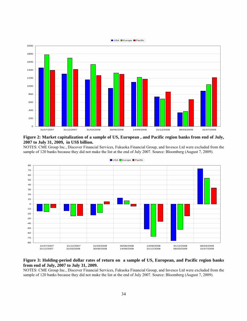
34

0

200

400

600

800

1000

1200

1400

1600

1800

2000

31/07/2007 31/12/2007 31/03/2008 30/06/2008 14/09/2008 31/12/2008 06/03/2009 31/07/2009

USA Europe Pacific

Figure 2: Market capitalization of a sample of US, European , and Pacific region banks from end of July, 2007 to July 31, 2009, in US$ billion. NOTES: CME Group Inc., Discover Financial Services, Fukuoka Financial Group, and Invesco Ltd were excluded from the sample of 120 banks because they did not make the list at the end of July 2007. Source: Bloomberg (August 7, 2009).

-80

-70

-60

-50

-40

-30

-20

-10

0

10

20

30

40

50

60

70

80

31/07/200731/12/2007

31/12/200731/03/2008

31/03/200830/06/2008

30/06/200814/09/2008

14/09/200831/12/2008

31/12/200806/03/2009

06/03/200931/07/2009

USA Europe Pacific

Figure 3: Holding-period dollar rates of return on a sample of US, European, and Pacific region banks from end of July, 2007 to July 31, 2009. NOTES: CME Group Inc., Discover Financial Services, Fukuoka Financial Group, and Invesco Ltd were excluded from the sample of 120 banks because they did not make the list at the end of July 2007. Source: Bloomberg (August 7, 2009).

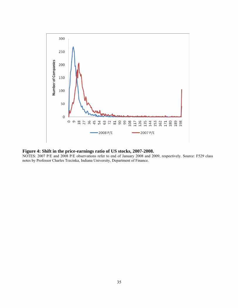
35

Figure 4: Shift in the price-earnings ratio of US stocks, 2007-2008. NOTES: 2007 P/E and 2008 P/E observations refer to end of January 2008 and 2009, respectively. Source: F529 class notes by Professor Charles Trzcinka, Indiana University, Department of Finance.

36

Cumulative Value of General Announcements in Banking System (in billion USD) from 1 to 15 October 2008

-

1,000

2,000

3,000

4,000

5,000

6,000

7,000

8,000

01/10/2008 02/10/2008 03/10/2008 04/10/2008 05/10/2008 06/10/2008 07/10/2008 08/10/2008 09/10/2008 10/10/2008 11/10/2008 12/10/2008 13/10/2008 14/10/2008 15/10/2008

Capital Injection Asset Purchase and Guarantees Debt Guarantees

Figure 5: Cumulative value of general announcements. October 1 through 15 2008. USD billions

37

Table 1: Rates of returns local currency and in dollars on selected US, European and Pacific region banks, in percent, end of July 2007 to July 31, 2009.

Area Country 31/07/2007 14/09/2008 31/07/2007 06/03/2009 31/07/2007 31/07/2009 LCU EXC USD LCU EXC USD LCU EXC USD

Europe AT -42.29 3.31 -40.38 -199.61 -7.86 -191.78 -104.68 4.06 -104.87 BE -54.67 3.31 -53.17 -287.72 -7.86 -272.96 -160.25 4.06 -162.69 DE -62.64 3.31 -61.40 -297.29 -7.86 -281.78 -207.92 4.06 -212.30 ES -43.14 3.31 -41.26 -101.61 -7.86 -101.48 -45.16 4.06 -42.93 FR -64.80 3.31 -63.64 -178.66 -7.86 -172.47 -104.34 4.06 -104.52 GR -42.61 3.31 -40.71 -161.66 -7.86 -156.81 -85.64 4.06 -85.06 IE -88.06 3.31 -87.66 -403.63 -7.86 -379.75 -239.22 4.06 -244.87 IT -42.65 3.31 -40.75 -134.29 -7.86 -131.59 -79.21 4.06 -78.37 PT -92.74 3.31 -92.50 -153.90 -7.86 -149.66 -121.45 4.06 -122.32 CH 13.52 5.88 20.19 14.64 4.21 19.47 15.44 11.94 29.22 DK -49.98 3.10 -48.43 -169.91 -8.01 -164.30 -77.06 3.97 -76.15 NO -30.46 1.44 -29.45 -126.41 -19.53 -121.25 -37.62 -5.14 -40.82 SE -45.72 -0.02 -45.73 -155.59 -31.50 -138.08 -72.10 -7.22 -74.11 UK -54.12 -12.92 -60.05 -233.67 -36.69 -184.63 -116.96 -19.76 -113.61Europe Total -50.92 1.05 -50.32 -175.20 -13.32 -163.14 -96.96 0.19 -96.53Pacific HK -12.04 0.39 -11.70 -77.53 0.92 -77.33 -12.71 0.98 -11.86 JP -43.66 10.26 -37.87 -109.63 19.65 -111.53 -78.37 23.12 -73.36 AU -30.34 -5.06 -33.87 -81.02 -29.35 -86.59 -40.53 -3.01 -42.32Pacific Total -30.34 3.42 -28.54 -92.49 1.89 -94.60 -48.28 9.76 -46.23USA US -39.27 0.00 -39.27 -166.92 0.00 -166.92 -93.74 0.00 -93.74USA Total -39.27 0.00 -39.27 -166.92 0.00 -166.92 -93.74 0.00 -93.74 NOTES: LCU = rate of return in local-currency units; EXC = depreciation/appreciation of the US dollar relative to the local currency; USD = rate of return in dollars; AT=Austria; BE=Belgium; CH=Switzerland; DE=Germany; DK=Denmark; ES=Spain; FR=France; GR=Greece; IE=Eire; IT=Italy; NO=Norway; PT=Portugal; SE=Sweden; UK=United Kingdom; AU=Australia; HK=Hong-Kong; JP=Japan; US=United States. CME Group Inc., Discover Financial Services, Fukuoka Financial Group, and Invesco Ltd were excluded from the sample of 120 banks because they did not make the list at the end of July 2007. Source: Bloomberg (August 7, 2009).

38

Table 2: Government interventions to support banks, by country and types through February 2009 (in million USD)

Country Public intervention in banks by country and typology

Total Bad Banks Convertible Bonds

Debt Guaranty

Equity Funding Nationalization

AT 0,00(a) 0,000BE 10,504 6,759 17,263CH 6,799 6,799DE 10,430 144,856 16,101 171,387EI 1,923 5,550 0,000 7,473FR 18,204 18,204IS 0,829 0,829LU 4,050 4,050NL 42,543 23,211 65,753UK 63,037 0,00(a) 63,037US 278,804 278,804

Total 42,543 21,278 146,779 392,200 30,799 633,599 NOTES: AT=Austria; BE=Belgium; CH=Switzerland; DE=Germany; DK=Denmark; ES=Spain; FR=France; GR=Greece; IE=Eire; IT=Italy; NO=Norway; PT=Portugal; SE=Sweden; UK=United Kingdom; AU=Australia; HK=Hong-Kong; JP=Japan; US=United States. (a) Government bought distressed banks for 2 euro in Austria and for free in UK. Source: Mediobanca (10 February 2009).

39

Table 3: Overview of commitments and outlays as of 10 June 2009* Capital Injections Debt Guarantees Asset purchase Asset Guarantees (1) Total

Euro billions and percentage points

% of GDP

(2008)

% of banking sector assets

(end-2008)

% of GDP

(2008)

% of banking sector assets

(end-2008)

% of GDP

(2008)

% of banking sector assets

(end-2008)

% of GDP

(2008)

% of banking sector assets

(end-2008) Euro billions

% of GDP

(2008)

% of banking sector assets

(end-2008) Australia Commitments – – – UNS UNS UNS – – – – – – UNS UNS UNS Outlays – – – 62 10.4 4.6 – – – – – – 62 10.4 4.6 Canada Commitments – – – UNS UNS UNS – – – – – – UNS UNS UNS Outlays – – – 0 0 0 – – – – – – – – – France Commitments 43 2.2 0.6 320 16.4 4.2 – – – 5 0.2 0.1 368 18.9 4.8 Outlays 28 1.4 0.4 72 3.7 0.9 – – – 5 0.2 0.1 104 5.3 1.4 Germany Commitments 80 3.2 1 420 16.9 5.3 UNS UNS UNS 200 8 2.5 700 28.1 8.9 Outlays 22 0.9 0.3 129 5.2 1.6 0 0 0 0 0 0 151 6.1 1.9 Italy Commitments 20 1.3 0.5 UNS UNS UNS – – – – – – UNS UNS UNS Outlays 10 0.6 0.3 0 0 0 – – – – – – 10 0.6 0.3 Japan Commitments 105 2.5 0.9 – – – 8 0.2 0.1 – – – 113 2.7 0.9 Outlays 3 0.1 0 – – – 0 0 0 – – – 3 0.1 0 Netherlands Commitments 37 6.2 1.7 200 33.6 9.0 – – – 28 4.7 1.3 265 44.6 11.9 Outlays 31 5.1 1.4 40 6.8 1.8 – – – 28 4.7 1.3 99 16.6 4.4 Spain Commitments UNS UNS UNS 100 9.1 3 – – – – – – UNS UNS UNS Outlays 0 0 0 31 2.8 0.9 – – – – – – 31 2.8 0.9 Switzerland Commitments 4 1.1 0.2 UNS UNS UNS 27 7.6 1.3 – – – UNS UNS UNS Outlays 4 1.1 0.2 0 0 0 27 7.6 1.3 – – – 31 8.7 1.5 United Kingdom Commitments 54 3.4 0.7 269 17.2 3.4 – – – 523 33.4 6.7 845 54 10.8 Outlays 54 3.4 0.7 113 7.2 1.4 – – – 523 33.4 6.7 690 44.1 8.8 United States Commitments 335 3 3.4 1,760 15.7 18 115 1 1.2 281 2.5 2.9 2,491 22.3 25.5 Outlays 237 2.1 2.4 271 2.4 2.8 36 0.3 0.4 281 2.5 2.9 825 7.4 8.4 Total commitments 677 2.6 1.1 3,131 11.8 5.2 150 0.6 0.3 1,036 3.9 1.7 4,994 18.8 8.3 Total outlays 387 1.5 0.6 719 2.7 1.2 64 0.2 0.1 836 3.2 1.4 2,006 7.6 3.3

* As of 10 June 2009 unless otherwise specified. UNS = unspecified amount; “–” = no program/action. Banking sector assets are consolidated data of: for Australia, banks, credit unions, building societies and corporations; for Canada, chartered banks; for Japan, depository corporations (banks and collectively managed trusts); for Switzerland, all domestic banks; for the five euro area countries and the United Kingdom, monetary financial institutions; and for the United States, commercial banks. Source: Panetta et al. (2009, Table 1.2).

40

Table 4: Overview of Policy Measures from 15 September 2008 to 1 June 2009. Amounts Pledged (bn)* Total* Note

Country Capital Injections

New Debt Issuance Guarantees Others Local

Currency (bn) EURbn % of GDP

Austria 15 85 100 100 37.0 Includes Dexia, Ethias, Fortis and KBC Belgium 19.6 19.6 19.6 5.9 Cyprus 2 2 2 12.8 Finland 4 50 54 54 30.1 France 24 320 344 344 18.2 Includes Dexia Germany 80 400 480 480 19.8 Greece 5 15 8 28 28 12.3 Ireland 7 400 407 407 213.5 Italy 12 40 52 52 3.4 Luxembourg 2.9 2.9 2.9 0.8 Includes Fortis, but not ING Netherlands 36.8 200 236.8 236.8 41.6 Illiquid Assets Facility Portugal 4 20 24 24 14.7 Slovenia 12 1 13 13 39.0 Spain 209 50 259 259 24.6 Includes guarantee on loan to Caja Castilla La Mancha Eurozone 197.8 1,711 99 2,028 1,955 21.0 Australia 8 8 4 0.7 Canada 218 125 343 259 22.3 Denmark 100 100 13.4 5.9 Plus losses over DKK35bn on bank liabilities Hungary 1.5** 1.5** 3.1** 2.3 2.2 Japan 13000 7691 20691 161.2 4.0 Norway 100 350 450 51.1 19.8 Qatar 6** 6** 4.7 8.8 SaudiArabia 3** 3** 2.4 0.8 SouthKorea 14.2** 100** 40.8** 155* 114.9 16.3 Sweden 65 1,500 1,565 145.8 51.0 Switzerland 6 6 4 1.0 Capitalisation of UBS Excludes Special Liquidity UK 678.1 250 635 963.1 1,059 68.7 Scheme (GBP200bn) but includes Asset Protection Scheme UAE 19** 19** 14.7 9.6 US 350 1,400*** 750**** 2,500 1,925 18.1 Does not include Fed’s facilities, such as the MMIFF but does include TALF NOTES: * Includes capital injections, asset buying and guarantees on debt issuance. Excludes deposit guarantees. ** In USD *** FDIC estimate of total size of unsecured debt falling under its guarantee. **** Includes USD500bn for PPIF, USD200bn for TALF, USD50bn for foreclosure prevention. Source: BNP Paribus.

41

Table 5: Timeline of general announcements (USD millions)

Date Country Measure

Total Capital Injection

Debt Guarantees

Asset Purchase and Guarantees Nationalization

21/04/08 UK 99,065 99,065 30/09/08 EI 14,081 14,081 02/10/08 GR 6,927 6,927 03/10/08 US 700,000 700,000 05/10/08 DK 0.1 0.1 07/10/08 ES 136,490 68,245 204,735 08/10/08 IT - -

UK 952,050 432,750 1,384,800 12/10/08 AU - -

PT 26,942 26,942 13/10/08 DE 53,884 545,669 53,884 653,437

FR 53,884 431,072 484,956 IT - - US 250,000 250,000

14/10/08 HK - - US 2,250,000 2,250,000

16/10/08 CH 60,000 60,000 17/10/08 BE - - 24/10/08 NO 51,071 51,071 26/10/08 AT 18,959 107,432 126,390 29/10/08 SE 195,277 195,277 03/11/08 AT 0 0 05/11/08 CH - - 28/11/08 IT - - 17/12/08 JP 136,612 136,612 18/01/09 DK 17,770 17,770 19/01/09 UK 73,685 73,685 03/02/09 JP 11,225 11,225 10/02/09 US - - - 12/02/09 EI 8,975 8,975 25/02/09 IT 15,277 15,277 26/02/09 UK 466,115 466,115 06/03/09 DE - - 17/03/09 JP 10,116 10,116 23/03/09 US 500,000 500,000 13/05/09 DE 272,240 272,240 09/06/09 US - - 22/07/09 HK - -

Total 2,392,877 3,981,426 1,645,394 - 8,019,696 NOTES: - = unspecified amount. Sources: Mediobanca, BIS-BdI, DLA Piper, International Capital Market Association, and websites of national Ministries of Treasury or Finance.

42

Table 6: Timeline of specific announcements (USD millions) Data Country Bank Measure

AP CI DG 14/03/2008 US JP Morgan Chase & Co. 2900030/09/2008 BE Dexia 4224.3

FR Dexia 4224.3 06/10/2008 DE Hypo Real Estate 6754013/10/2008 UK Lloyds TSB 22900.7

RBS 26942 27/10/2008 BE KBC 4356.1 28/10/2008 US Bank of America 15000

Bank of New York Mellon 3000 Citigroup 25000 Goldman Sachs Group 10000 JP Morgan Chase & Co. 25000 Morgan Stanley 10000 State Street Corp. 2000 Wells Fargo Bank 25000

03/11/2008 DE Commerzbank 10429.58 13/11/2008 DE Hypo Real Estate 2505217/11/2008 US BB&T Corp. 3133.64

Comerica 2250 First Horizon National Corp. 866.54 Huntington Bancshares 1398.071 Key Corp. 2500 Marshall & Ilsley Corp. 1715 Northern Trust Corp 1576 Regions Financial Corp 3500 Sun Trust Banks 3500 US Bancorp 6599 Zions Bancorporation 1400

21/11/2008 DE Hypo Real Estate 2506223/11/2008 US Citigroup 262000 09/12/2008 DE Hypo Real Estate 1293711/12/2008 FR BNP Paribas 3389.97

Crédit Agricole 3988.2 Societé Générale 2259.98

21/12/2008 EI Allied Irish Banks 2775 Bank of Ireland Group 2775

23/12/2008 US M&T BankCorp 600 31/12/2008 US CIT Group 2330

Citigroup 20000 Fifth Third Bancorp 3408 PNC Financial Services Group 7579.2 Sun Trust Banks 1350

09/01/2009 US American Express Company 3388.89 Bank of America 10000

14/01/2009 AT Erste Group Bank 7904.416/01/2009 US Bank of America 97000

Citigroup 301000 20/01/2009 DE Hypo Real Estate 15535.211/02/2009 DE Hypo Real Estate 1289312/02/2009 EI Allied IrishBanks 1923.3

Bank of Ireland Group 1923.3 26/02/2009 UK Royal Bank of Scotland 16593.2

43

27/02/2009 AT Erste Group Bank 3418.74 07/03/2009 UK LloydsTSB 329524 10/03/2009 IT Banco Popolare 1849.04 13/03/2009 US Discover Financial Services 1224.558 18/03/2009 IT Unicredit Group 2622 20/03/2009 IT Intesa Sanpaolo 5426.4 24/03/2009 IT Banca Popolare di Milano 676.2 27/03/2009 IT Banca Monte dei Paschi di Siena 2528.14 31/03/2009 FR BNP Paribas 6763.11 13/04/2009 US Wells Fargo Bank 2873 17/04/2009 US Bank of America 798.9

Total 362671.9 960151.1046 195923.6 NOTES: AP = Asset Guarantees and Purchase; CI = Capital Injection; DG = Debt Guarantees. Source: Mediobanca, BIS-BdI, and CNN Money.

44

Table 7: Effects of general and specific announcements on banks’ rates of return; fixed effects

COEFFICIENT . All Announcements . . Announcements by type .

(1) (2) (3) (4) (5) (6) (7) (8) All periods Subperiod 1 Subperiod 2 Subperiod 3 All periods Subperiod 1 Subperiod 2 Subperiod 3

Rm 1.405*** 1.355*** 1.331*** 1.731*** 1.405*** 1.355*** 1.332*** 1.732*** SIZE 0.00215*** 0.00324*** 0.0198*** 0.00217 0.00211*** 0.00324*** 0.0198*** 0.00251 G 0.00666*** -0.00183 0.00465*** 0.00290* GAP 0.00345** 0 0.00455** -0.0128 GCI 0.00481*** -0.00183 0.00216 0.00429** GDG 0.00614*** 0 0.00443 -0.00916 S -0.0119*** 0.0179* -0.0136*** 0.00355 SAP -0.0109 0 -0.0243 0.00607 SCI -0.0137*** 0 -0.0156*** 0.00308 SDG -0.00103 0.0179* 0.00637 0 Constant -0.0202*** -0.0315*** -0.180*** -0.0187 -0.0198*** -0.0315*** -0.180*** -0.0217 Observations 61,467 34,354 14,697 12,416 61,467 34,354 14,697 12,416 Number of bank 120 120 120 120 120 120 120 120 Adjusted R2 0.392 0.428 0.320 0.328 0.392 0.428 0.321 0.328 F-Test 9,984 6,814 2,544 1,547 4,993 6,814 1,273 885.3 (0.000) (0.000) (0.000) (0.000) (0.000) (0.000) (0.000) (0.000) Hausman Test 36.00 23.61 208.8 47.71 36.81 23.61 284.6 -99.81(a) (0.000) (0.000) (0.000) (0.000) (0.000) (0.000) (0.000) (1.000) WALD GSx=0 52.06 1.618 12.72 1.562 18.20 1.618 5.560 1.907 (0.000) (0.198) (0.000) (0.210) (0.000) (0.198) (0.000) (0.0896) F-Test GAP=GCI 0.512 - 0.457 2.719 (0.474) (0.499) (0.0991) F-Test GAP=GDG 1.677 - 0.00150 0.0927 (0.195) (0.969) (0.761) F-Test GCI=GDG 0.382 - 0.301 4.237 (0.537) (0.583) (0.0395) F-Test GAP=GCI 0.0959 - 0.222 0.0329 (0.757) (0.638) (0.856) F-Test GAP=GDG 0.856 - 2.134 0.172 (0.355) (0.144) (0.678) F-Test GCI=GDG 3.584 - 3.747 0.163 (0.0583) (0.0529) (0.687) CAR=G*7 4.66% - 3.26% 2.03% CAR=GAP*7 2.42% - 3.19% - CAR=GC I *7 3.37% - - 3.00% CAR=GDG*7 4.30% - - - CAR=S*5 -5.95% 8.95% -6.80% - CAR=SAP*5 - - - - CAR=SCI*5 -6.85% - -7.80% - CAR=SDG*5 - 8.95% - - NOTES: All estimations with fixed effects. See text for sub-period. Rm = rate of market return; SIZE = ln(Market Capitalization in million USD); G = general announcement; S = specific announcement; AP = Asset Guarantees and Purchase; CI = Capital Injection; DG = Debt Guarantees; Hausman Test vs. random effect model; GSx = all general and specific announcements; CAR = Cumulative Abnormal Return. (a) fails to meet asymptotic assumption. *** p<0.01, ** p<0.05, * p<0.1. P-values of tests in parentheses.

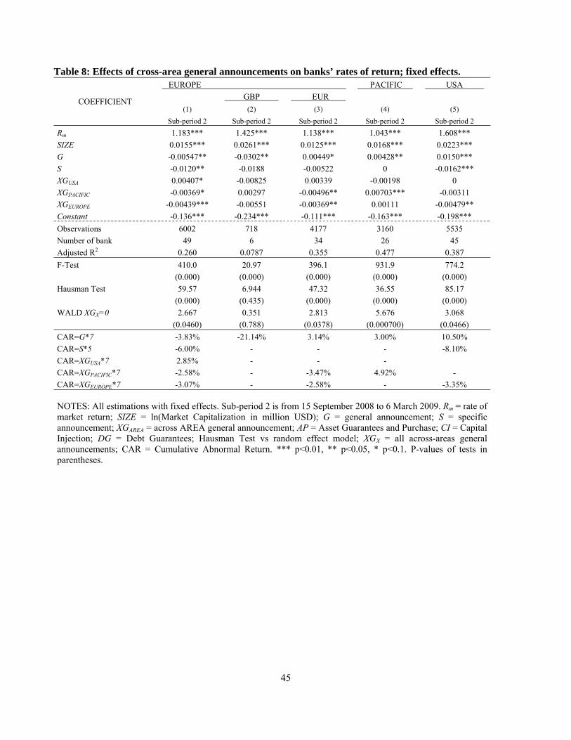
45

Table 8: Effects of cross-area general announcements on banks’ rates of return; fixed effects.

COEFFICIENT

. EUROPE . . PACIFIC . . USA . . GBP . . EUR .

(1) (2) (3) (4) (5) Sub-period 2 Sub-period 2 Sub-period 2 Sub-period 2 Sub-period 2

Rm 1.183*** 1.425*** 1.138*** 1.043*** 1.608*** SIZE 0.0155*** 0.0261*** 0.0125*** 0.0168*** 0.0223*** G -0.00547** -0.0302** 0.00449* 0.00428** 0.0150*** S -0.0120** -0.0188 -0.00522 0 -0.0162*** XGUSA 0.00407* -0.00825 0.00339 -0.00198 0 XGPACIFIC -0.00369* 0.00297 -0.00496** 0.00703*** -0.00311 XGEUROPE -0.00439*** -0.00551 -0.00369** 0.00111 -0.00479** Constant -0.136*** -0.234*** -0.111*** -0.163*** -0.198*** Observations 6002 718 4177 3160 5535 Number of bank 49 6 34 26 45 Adjusted R2 0.260 0.0787 0.355 0.477 0.387 F-Test 410.0 20.97 396.1 931.9 774.2 (0.000) (0.000) (0.000) (0.000) (0.000) Hausman Test 59.57 6.944 47.32 36.55 85.17 (0.000) (0.435) (0.000) (0.000) (0.000) WALD XGX=0 2.667 0.351 2.813 5.676 3.068 (0.0460) (0.788) (0.0378) (0.000700) (0.0466) CAR=G*7 -3.83% -21.14% 3.14% 3.00% 10.50% CAR=S*5 -6.00% - - - -8.10% CAR=XGUSA*7 2.85% - - - CAR=XGPACIFIC*7 -2.58% - -3.47% 4.92% - CAR=XGEUROPE*7 -3.07% - -2.58% - -3.35% NOTES: All estimations with fixed effects. Sub-period 2 is from 15 September 2008 to 6 March 2009. Rm = rate of market return; SIZE = ln(Market Capitalization in million USD); G = general announcement; S = specific announcement; XGAREA = across AREA general announcement; AP = Asset Guarantees and Purchase; CI = Capital Injection; DG = Debt Guarantees; Hausman Test vs random effect model; XGX = all across-areas general announcements; CAR = Cumulative Abnormal Return. *** p<0.01, ** p<0.05, * p<0.1. P-values of tests in parentheses.

46

Table 9: Effects of cross-bank specific announcements on banks’ rates of return; OLS

COEFFICIENT

BANK OF AMERICA CITIGROUP JPMORGAN WELLS

FARGO GOLDMAN

SACHS AMERICAN

EXPRESS MORGAN STANLEY

(1) (2) (3) (4) (5) (6) (7)

Sub-period 2 Sub-period 2 Sub-period 2 Sub-period 2 Sub-period 2 Sub-period 2 Sub-period 2Rm 2.269*** 2.235*** 1.760*** 1.846*** 1.499*** 1.664*** 2.570*** SIZE 0.00483 0.00986 0.0157 0.0176 0.00719 0.00824 -0.00340 G 0.0153 0.00266 0.00490 0.00187 0.00679 -0.00103 0.0141 S -0.0601** -0.0133 -0.0156 0.0537** -0.0500* 0.00734 -0.0288 XSBANK OF AMERICA -0.0719** -0.00767 -0.0272 -0.0212 -0.00496 -0.0178 XSCITIGROUP -0.0223 -0.0259* -0.0254 0.0162 -0.000504 0.00224 XSJPMORGAN -0.0333 0 -0.0246 0 -0.0526** 0 XSWELLS FARGO 0.0846*** 0.0845** 0.0237 0.00375 0.0505*** -0.00715 XSGOLDMAN SACHS 0 -0.0333 0 0 0 0 XSAMERICAN EXPRESS 0.0315 0.0546 0.00607 0.0213 0.0154 0.0418 XSMORGAN STANLEY 0 0 0 0 0 0 Constant -0.0497 -0.0981 -0.179 -0.196 -0.0749 -0.0824 0.0382 Observations 227 227 227 227 227 227 227 R2 0.539 0.435 0.588 0.511 0.579 0.668 0.576 F-Test 31.84 20.96 38.81 28.45 37.46 54.91 37.00 (0.000) (0.000) (0.000) (0.000) (0.000) (0.000) (0.000) WALD X-ANNBANKS=0 2.673 2.555 1.676 2.689 0.763 2.429 0.348 (0.0330 (0.0398) (0.157) (0.0321) (0.550) (0.0487) (0.845) CAR=G*7 - - - - - - - CAR=S*5 -30.05% - - 26.85% -25.00% - -30.05% CAR=XSBANK OF AMERICA*5 -35.95% - - - - - CAR=XSCITIGROUP*5 - -12.95% - - - - CAR=XSJPMORGAN*5 - - - - -26.30% - CAR=XSWELLS FARGO*5 42.30% 42.25% - - 25.25% 42.30% CAR=XSGOLDMAN SACHS*5 - - - - - - CAR=XSAMERICAN EXPRESS*5 - - - - - - CAR=XSMORGAN STANLEY*5 - - - - - - NOTES: All estimations are OLS. Sub-period 2 is from 15 September 2008 to 6 March 2009. Rm = rate of market return; SIZE = ln(Market Capitalization in million USD); G = general announcement; S = specific announcement; Hausman Test vs random effect model; XSBANKS = across BANKS specific announcements; CAR = Cumulative Abnormal Return. *** p<0.01, ** p<0.05, * p<0.1. P-values of tests in parentheses.

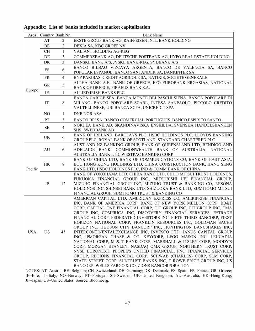
47

Appendix: List of banks included in market capitalization

Area Country Bank Nr. Bank Name

Europe

AT 2 ERSTE GROUP BANK AG, RAIFFEISEN INTL BANK HOLDING BE 2 DEXIA SA, KBC GROEP NV CH 1 VALIANT HOLDING AG-REG DE 3 COMMERZBANK AG, DEUTSCHE POSTBANK AG, HYPO REAL ESTATE HOLDING DK 3 DANSKE BANK A/S, JYSKE BANK-REG, SYDBANK A/S

ES 6 BANCO BILBAO VIZCAYA ARGENTA, BANCO DE VALENCIA SA, BANCO POPULAR ESPANOL, BANCO SANTANDER SA, BANKINTER SA

FR 4 BNP PARIBAS, CREDIT AGRICOLE SA, NATIXIS, SOCIETE GENERALE

GR 5 ALPHA BANK A.E., BANK OF GREECE, EFG EUROBANK ERGASIAS, NATIONAL BANK OF GREECE, PIRAEUS BANK S.A.

IE 1 ALLIED IRISH BANKS PLC

IT 8 BANCA CARIGE SPA, BANCA MONTE DEI PASCHI SIENA, BANCA POPOLARE DI MILANO, BANCO POPOLARE SCARL, INTESA SANPAOLO, PICCOLO CREDITO VALTELLINESE, UBI BANCA SCPA, UNICREDIT SPA

NO 1 DNB NOR ASA PT 3 BANCO BPI SA, BANCO COMERCIAL PORTUGUES, BANCO ESPIRITO SANTO

SE 4 NORDEA BANK AB, SKANDINAVISKA ENSKILDA, SVENSKA HANDELSBANKEN SHS, SWEDBANK AB

UK 6 BANK OF IRELAND, BARCLAYS PLC, HSBC HOLDINGS PLC, LLOYDS BANKING GROUP PLC, ROYAL BANK OF SCOTLAND, STANDARD CHARTERED PLC

Pacific

AU 6 AUST AND NZ BANKING GROUP, BANK OF QUEENSLAND LTD, BENDIGO AND ADELAIDE BANK, COMMONWEALTH BANK OF AUSTRALIA, NATIONAL AUSTRALIA BANK LTD, WESTPAC BANKING CORP

HK 8 BANK OF CHINA LTD, BANK OF COMMUNICATIONS CO, BANK OF EAST ASIA, BOC HONG KONG HOLDINGS LTD, CHINA CONSTRUCTION BANK, HANG SENG BANK LTD, HSBC HOLDINGS PLC, IND & COMM BANK OF CHINA

JP 12

BANK OF YOKOHAMA LTD, CHIBA BANK LTD, CHUO MITSUI TRUST HOLDINGS, FUKUOKA FINANCIAL GROUP INC., MITSUBISHI UFJ FINANCIAL GROUP, MIZUHO FINANCIAL GROUP INC, MIZUHO TRUST & BANKING CO, RESONA HOLDINGS INC, SHINSEI BANK LTD, SHIZUOKA BANK LTD, SUMITOMO MITSUI FINANCIAL GROUP, SUMITOMO TRUST & BANKING CO

USA US 45

AMERICAN CAPITAL LTD, AMERICAN EXPRESS CO, AMERIPRISE FINANCIAL INC, BANK OF AMERICA CORP, BANK OF NEW YORK MELLON CORP, BB&T CORP, CAPITAL ONE FINANCIAL CORP, CIT GROUP INC, CITIGROUP INC, CMA GROUP INC, COMERICA INC, DISCOVERY FINANCIAL SERVICES, E*TRADE FINANCIAL CORP, FEDERATED INVESTORS INC, FIFTH THIRD BANCORP, FIRST HORIZON NATIONAL CORP, FRANKLIN RESOURCES INC, GOLDMAN SACHS GROUP INC, HUDSON CITY BANCORP INC, HUNTINGTON BANCSHARES INC, INTERCONTINENTALEXCHANGE INC, INVESCO LTD, JANUS CAPITAL GROUP INC, JPMORGAN CHASE & CO, KEYCORP, LEGG MASON INC, LEUCADIA NATIONAL CORP, M & T BANK CORP, MARSHALL & ILSLEY CORP, MOODY'S CORP, MORGAN STANLEY, NASDAQ OMX GROUP, NORTHERN TRUST CORP, NYSE EURONEXT, PEOPLE'S UNITED FINANCIAL, PNC FINANCIAL SERVICES GROUP, REGIONS FINANCIAL CORP, SCHWAB (CHARLES) CORP, SLM CORP, STATE STREET CORP, SUNTRUST BANKS INC, T ROWE PRICE GROUP INC, US BANCORP, WELLS FARGO & CO, ZIONS BANCORPORATION

NOTES: AT=Austria, BE=Belgium; CH=Switzerland; DE=Germany; DK=Denmark; ES=Spain; FR=France; GR=Greece; IE=Eire; IT=Italy; NO=Norway; PT=Portugal; SE=Sweden; UK=United Kingdom; AU=Australia; HK=Hong-Kong; JP=Japan; US=United States. Source: Bloomberg.