Relationship between Currency Carry Trades and Gold Returns

A quantitative study of G-10 currencies: correlation and spillover

effects for the last two decades.

Authors: Johannes Hornbrinck

Jonas Olausson

Supervisor: Janne Äijö

Students

Umeå School of Business and Economics

Spring semester 2014

Master thesis, two-year, 15 hp

Acknowledgement

As we are approaching the end of the writing process for this thesis we would like to take the

time to give thanks to the people that in any way have been involved in the conduction of it.

Special thanks go to our supervisor, Janne Äijö, for providing valuable inputs throughout the

process of this research.

Sincerely

Johannes Hornbrinck Jonas Olausson

May, 2014

iii

Abstract

Currency carry trade is an investment strategy that recently started gaining a lot of interest not

only among investors and financial institutions but also academically. One of the underlying

theoretical assumptions regarding the mechanisms of the foreign exchange market, the

Uncovered Interest Parity has frequently been disproved in practice which has led to the

conclusion that carry trade is profitable in practice. The function of a carry trade strategy is

that a short position is taken in a low interest rate currency to finance a long position in

another currency offering higher yields. This thesis is adding to the existing literature that is

explaining the characteristics of currency carry trade but is adopting a different approach than

most other recent researches that has focused on identifying especially risk factors. Gold as a

financial asset has also received much attention largely due to its, contrarily to other asset

classes, low dependence on macroeconomic factors. This makes gold desirable to diversify

portfolios and decreasing overall risks. By investigating how the returns of currency carry

trades and gold relates to each other an increased understanding in how carry trades can be

beneficially included in managing portfolios are developed. Looking at a currency carry trade

index, Deutsche Bank’s G10 Currency Future Harvest index, and the development of the gold

price at the London bullion market for the 20 year period of 1993-2013 this research is

exploring correlation, mean and volatility spillover effects. Spearman’s correlation, Vector

Autoregression and a diagonal BEKK GARCH model are employed to test these effects. It

also investigates if gold possesses hedge, diversifier and safe haven characteristics when

combined with carry trades as it has been found to do with stock markets. This is determined

by a regression analysis and supplemented by a portfolio simulation.

This thesis found that there is a low positive correlation between the returns of gold and

currency carry trades and that there is spillover effects as well between the two in both returns

and volatility. This in addition to the regression analysis and portfolio analysis determined

that there are diversification benefits by adding gold to a portfolio consisting of currency

carry trade in the form of higher risk adjusted returns. However special caution has to be

taken to the spillover effects as these complicate the relationship between the returns of the

two variables and especially the volatility spillover effects slightly decreases the potential

diversification benefit. The regression analysis concluded that gold work as a diversifier for

carry trade but could not determine if it also exhibited hedge or safe haven characteristics.

These findings pushes the existing understanding of carry trades forward and adds to focus of

matching carry trades within a portfolio which could have implications to more efficiently

match risks and returns by combining several asset classes in portfolio management.

iv

Glossary

G-10

The term G-10 is a group of the ten most actively traded currencies which are also therefore

considered the most liquid and in extension, safe currencies to trade in.

Spillover

Spillover refers to the effect of where a situation unintentionally affects another. It is thus a

secondary effect that arises from and is to some extent caused by a primary effect. Although

these effects are separated by time and space.

Correlation

Correlation corresponds and measures to what extent two random variables vary in the same

directions. Variables that are considered highly correlated tend to often move increase or

decrease in value at the same time while uncorrelated move independently of each other.

Variance

Variance in finance concerns how much the value of a certain asset fluctuates over a time

period. This is largely considered in regard to risk as assets associated with higher fluctuations

are more unpredictable and more risky.

Safe haven

Safe haven is regarded as something or someplace relatively safe to turn to when all else

seems risky and turbulent, thus as the climate becomes more unpredictable and unsafe the safe

havens are still being considered calm and are therefore associated with lower risk (Baur &

McDermott, 2010, p. 1893).

v

Table of Contents Acknowledgement ...................................................................................................................... ii

Abstract ..................................................................................................................................... iii

Glossary ..................................................................................................................................... iv

Table of Contents ....................................................................................................................... v

List of Figures ......................................................................................................................... viii

List of Tables ........................................................................................................................... viii

1. Introduction ............................................................................................................................ 1

1.1 Problem Background ........................................................................................................ 1

1.2 Research Questions .......................................................................................................... 3

1.3 Research Purpose ............................................................................................................. 3

1.4 Research Gap .................................................................................................................... 3

1.5 Research Contributions .................................................................................................... 4

1.6 Delimitations .................................................................................................................... 5

2. Research Methodology ........................................................................................................... 7

2.1 Preconceptions & Choice of Subject ................................................................................ 7

2.2 Research Philosophy ........................................................................................................ 7

2.2.1 Ontology .................................................................................................................... 8

2.2.2 Epistemology ............................................................................................................. 8

2.3 Research Approach .......................................................................................................... 9

2.4 Research Method ............................................................................................................ 10

2.5 Research Design ............................................................................................................. 11

2.6 Literature & Data Sources .............................................................................................. 11

2.7 Quality Criterion ............................................................................................................ 12

2.8 Summary of Research Methodology .............................................................................. 14

3. Theoretical Framework ........................................................................................................ 15

3.1 Uncovered Interest Rate Parity....................................................................................... 15

3.2 Covered Interest Rate Parity .......................................................................................... 15

3.3 Currency Carry Trade ..................................................................................................... 16

3.4 Carry Trades and Volatility ............................................................................................ 17

3.5 Currency Carry Trades and Stock Markets .................................................................... 18

3.6 Characteristics of Gold ................................................................................................... 19

3.7 Portfolio Theory ............................................................................................................. 20

3.7.1 Risk .......................................................................................................................... 20

3.7.2 Modern Portfolio Theory ........................................................................................ 21

vi

3.7.3 Sharpe Ratio ............................................................................................................ 22

3.7.4 Behavioral finance ................................................................................................... 22

3.8 G-10 Currencies ............................................................................................................. 24

3.9 Asset Characteristics for portfolio diversification.......................................................... 25

4. Practical Methodology ......................................................................................................... 26

4.1 Data sample .................................................................................................................... 26

4.2 Time horizon .................................................................................................................. 26

4.3 Return Calculations ........................................................................................................ 27

4.4 Correlation ...................................................................................................................... 27

4.5 Spillover Effects ............................................................................................................. 28

4.5.1 Return Spillover ...................................................................................................... 29

4.6 OLS Regression .............................................................................................................. 31

4.7 Hypotheses ..................................................................................................................... 33

4.7.1 Correlation Testing .................................................................................................. 34

4.7.2 Spillover Effects ...................................................................................................... 34

4.7.3 Regression Testing .................................................................................................. 34

5. Empirical Findings ............................................................................................................... 35

5.1 Descriptive Statistics ...................................................................................................... 35

5.1.1 Development ........................................................................................................... 35

5.1.2 Return Distributions ................................................................................................ 36

5.2 Correlation ...................................................................................................................... 38

5.3 Spillover Effect .............................................................................................................. 39

5.3.1 Mean Spillover ........................................................................................................ 39

5.3.2 Volatility Spillover .................................................................................................. 41

5.4 Regression ...................................................................................................................... 44

5.5 Portfolio Simulation ....................................................................................................... 45

5.6 Hypotheses Testing ........................................................................................................ 46

6. Discussion ............................................................................................................................ 49

6.1 Summary Results ............................................................................................................ 49

6.2 Carry-trade and Gold Correlation................................................................................... 50

6.3 Spillover Effects ............................................................................................................. 51

6.4 Diversification Benefits of Gold .................................................................................... 52

7. Conclusion & Recommendations ......................................................................................... 54

7.1 Conclusion ...................................................................................................................... 54

7.2 Contributions .................................................................................................................. 55

vii

7.3 Reliability & Validity ..................................................................................................... 55

7.4 Ethical Concerns ............................................................................................................ 57

7.5 Suggestions for further research ..................................................................................... 58

Reference List .......................................................................................................................... 59

Appendix 1 – Normality tests ................................................................................................... 64

Appendix 2 – AIC Lag test ...................................................................................................... 65

viii

List of Figures Figure 1: Deduction & Induction Process ................................................................................ 10

Figure 2: Research Methodology ............................................................................................. 14

Figure 3: Gold & Carry Trade Development ........................................................................... 35

Figure 4: Gold Return Volatility .............................................................................................. 36

Figure 5: Carry Returns Volatility ........................................................................................... 37

Figure 6: Return Variance ........................................................................................................ 44

Figure 7: Portfolio Simulation .................................................................................................. 45

List of Tables Table 1: G-10 Currencies ......................................................................................................... 25

Table 2: Deutsche Bank Carry Index ....................................................................................... 27

Table 3: Total Returns .............................................................................................................. 36

Table 4: Descriptive Statistics .................................................................................................. 36

Table 5: Normality Test ........................................................................................................... 38

Table 6: Spearman's Correlation .............................................................................................. 38

Table 7: Unit Root Test ............................................................................................................ 39

Table 8: VAR Gold Returns ..................................................................................................... 40

Table 9: VAR Carry Returns .................................................................................................... 41

Table 10: GARCH Lag Test ..................................................................................................... 42

Table 11: BEKK GARCH Test ................................................................................................ 42

Table 12: Regression Analysis ................................................................................................. 44

Table 13: Portfolio Simulation ................................................................................................. 46

1

1. Introduction This chapter introduces the research and research topic. It begins with providing the

background to the problem at hand which summarizes the current knowledge regarding

the subject and what is not yet known. Sequentially the research question is presented

and the core method for how the research is going to be conducted. Contributions and

limitations of this research are stated and the chapter is concluded with a disposition of

the thesis.

1.1 Problem Background

Currency carry trades and the failure of the uncovered interest rate parity have puzzled

researchers over the world. The focus have then started to shift towards finding the

driving risk factors related to this in order to try to understand if the excess returns can

be justified.

Currency carry trades or just carry trade is an investment strategy where you are

borrowing in low-yielding currencies and lend (invest) in high yielding currencies. The

theoretical basis is the uncovered interest rate parity which suggests that it should not be

possible to attain positive returns with this kind of trading (Rosenberg, 2013, p. 13).

Since the difference in the interest rates will be canceled out by a

depreciation/appreciation in the exchange rate. This works according to the principle of

no arbitrage, however there are a considerable amount of empirical evidence that have

found that this is not necessarily the case (Clarida et al., 2009).

This discrepancy have led researchers into considering that the failure of the uncovered

interest rate parity could be attributable to a risk premium that might have to be

incorporated due to accommodate for the different risk associated with different

countries. Researchers have extensively been trying to shed light on how to evaluate the

risk associated to these investments. There have been a lot of research trying to solve

this issue but these have yet been unsuccessful able to find a good pricing model that

incorporates the correct risk associated to it (Bhansali, 2007; Clarida et al., 2009;

Brunnermeier et al., 2008; Cenedese et al., 2014).

Banks have introduced carry trade indices in light of the growing interest in currency

carry trades and the area getting ever increasingly coverage as well as an ever larger

increase in the legitimacy as a solid investment strategy (Arnold et al., 2006). Despite

its popularity there is a lack of consensus on the actual attributes of the strategy and

how it relates to other investments strategies, academic literature have especially had

trouble identifying the risk drivers associated to the carry trade strategy (Burnside,

2011a, p. 853). Thus obstructing the possibility of effectively managing such an

investment by introducing it to portfolios consisting of other assets and the benefits

carry trades could bring to a portfolio.

Currency carry trades have been found to behave differently depending on the state of

exchange rate volatility (Bhansali, 2007; Clarida et al., 2009). Empirical research has

found that it systematically generates positive returns in states of low volatility and

considerably large negative returns in high volatility states (Clarida et al., 2009, p. 20).

This have been linked to a lot of investors unwinding their carry trade positions in

2

turbulent times, resulting in a steep appreciation of the low-yielding funding currencies

and the large losses for investors (Brunnermeier et al., 2008, p. 29; Clarida et al., 2009).

For a carry trade portfolio it has been proven that there is a diversification benefit of

including different currencies (Clarida et al., 2009, p. 8; Lustig & Verdelhan, 2007, p.

113). However due to the behavior in different volatility regimes it have not been much

research regarding how to handle and potentially hedge a carry trade portfolio in these

high volatility states.

Since there is no general consensus on how to determine and appropriately appraise the

risks, it does not exist a definite way in how to eliminate some downside risk by

sacrificing some return. As a common measure for measuring the risk/return for the

carry trades have been the Sharpe ratio. This is a way to analyze and more specifically

compare the investments performance with respect to its respective risk.

Previous researches on carry trades have revolved a lot around currency carry trades as

an individual asset class. However as Das et al. (2012, p. 256) states it should receive

more attention for the purpose of portfolio management. Since it possesses several

favorable characteristics as it displays low standard deviation and also shows modest

correlation to equity-based assets (Das et al., 2012, p. 256).

As for the relationship between various currencies and the equity market it has also

shown different characteristics depending on the features of the currency. High yielding

currencies has proven to be positively related to the returns of the stock market, while

low yielding on the other hand has demonstrated negative relationships (Katecheos,

2011, p. 558). This further defies the uncovered interest rate parity as currencies

generally has shown to move in the opposite direction of what this condition suggest,

increasing potential returns from currency carry trades even more. The relationship is

also dependent on the interest rate differentials between the different currencies where

larger differentials suggest a stronger relationship and vice versa when the differentials

are lower (Katecheos, 2011, p. 558).

Gold is an asset class that historically has been regarded as a safe-haven due to its

property of being largely uncorrelated to stocks and bonds on average. Safe-haven is

distinguished from hedge or diversifier, since it has the property of retaining or

increasing in value even in times of market turmoil (Baur & McDermott, 2010, p.

1893). The purpose and benefits of safe haven assets is then to be invested in order to

limit the losses that might be incurred in these situations. Baur & Lucey (2010, p. 228)

discovered empirical evidence that gold act as a safe haven for stocks.

Considering that there is a recently increased academic interest in currency carry trades

with many articles dating back just a few years it is interesting to investigate the

currency carry trades characteristics in regard to portfolio management (Bhansali, 2007;

Clarida et al., 2009; Brunnermeier et al., 2008). Currencies have shown modest

correlation with the stock market, given that carry trades share the characteristics of

yielding very negative returns in states when the exchange rate market are experiencing

high volatility. This effect might to some extent be able to be mitigated by gold

investment due to its safe-haven characteristics. This is an issue that as far as we have

found lacks empirical evidence and is therefore an area of interest and in need of further

investigation.

3

1.2 Research Questions

Building on the problem background and previous research we find that there is a lot of

researches with emphasis on the risk drivers for currency carry trades. A less researched

area regarding currency carry trades are the relation to other financial assets. We found

it interesting to further explore potential portfolio diversification of carry trades. We

intend to explore this in relation how carry trades returns and gold returns relate to each

other. In order to enable us to achieve this we have develop the following research

questions:

Is there a co-movement between currency carry trade returns and gold price returns?

Are there any spillover effects between currency carry trade returns and gold price

returns?

1.3 Research Purpose

The purpose of the research is to investigate the relationship in the movements of

currency carry trade returns and gold returns. Firstly, this will be done by establishing

the correlation between carry trade returns and gold returns. Secondly, we are going to

extend the analysis of this relationship by testing the mean and volatility spillover

effects. Thirdly, we are going to investigate the potential safe-haven, hedge and

diversifier properties of gold in relation to a currency carry trade portfolio by employing

a regression model. Furthermore the regression analysis will also help us to investigate

the relationship between these assets in different volatility states.

1.4 Research Gap

Most of earlier research for currency carry trades have been centered round identifying

the specific risk factors that are associated to this investment vehicle. In order to

understand what drives the excess returns and if these excess returns associated with the

currency carry trade is fair given the risks undertaken (Clarida et al., 2009; Bhansali,

2007; Brunnermeier et al., 2008). These researches have focused on currency carry

trades as an individual asset type and little attention has been given to carry trades as an

asset class among others in a portfolio.

Lustig & Verdelhan (2007, p. 94-95) looked a bit more into the portfolio aspects of

currency carry trades when they investigated the diversification benefits of including

additional currencies into a currency portfolio. Their findings that a well-designed

currency portfolio can eliminate some of this hypersensitive risk that individual

currencies experience some that there are potential benefits of diversifying your

currency carry trade portfolio.

This research intends to contribute to the academic field by fulfilling the research gap of

currency carry trades portfolios aspects by providing empirical evidence of how

4

currency carry trade returns relate to the returns characteristics of other asset classes, in

this case gold price returns.

1.5 Research Contributions

As stated previously this study, on the contrary to previous studies, will focus more on

carry trades as an asset class for portfolio management. This is something that have

been lacking since most of the earlier studies have focused on identifying the risk with

the carry trades as an individual asset rather than how it relates to other assets.

Building from Clarida et al. (2009) findings of the negative returns associated with

carry trade returns in high volatility states, our research will investigate how gold relates

to the currency carry trades. To during the chosen time period generate an

understanding whether gold can be used to help offset some of these downside risks.

Lustig & Verdelhan (2007, p. 94-95) findings established that there are some

diversification benefits by a well-designed currency portfolio where we want to

investigate if this can be extended further to other assets, which in this case is gold due

to its’ desirable safe haven characteristics with the equity markets.

The results can help narrow down or pinpoint more factors that can relate to the

movements of the currency carry trades returns. Additionally explaining how currency

carry trade returns relates to other assets help will not only shed further light on the

behavior of carry trades and allow for more appropriate allocation in portfolios, but also

provides another aspect in explaining the uncovered interest rate parity puzzle. The

academically derived parity condition regarding economics and the mechanisms of the

foreign rate market that surprisingly and frequently been disproved empirically.

It will also extend on the research of Das et al. (2013) which found that currency carry

trades can be matched with other asset classes in a portfolio for better risk-adjusted

returns. By investigating how carry trade relates to gold implications regarding how to

match them to effectively manage risks can be made.

This can be of help for currency fund managers since it can help them better understand

how to manage their portfolios during different risk scenarios of the market. This could

further explain the behavior of currency carry trades and help determine how the

associated downside risks in more turbulent market environments better can be handled.

Empirically we will contribute to how currency carry trades relate towards the gold

price returns. A relationship that has not as far as we could establish receive any

significant academic attention beforehand. It can then also be seen if the inclusion of

other assets, other than including more currencies which has been researched be Lustig

& Verdelhan (2007), within the carry trade portfolios can help better handle the

downside risk and generate a portfolio with a better trade-off between the risk and

return.

5

1.6 Delimitations

This study is limited to testing carry trade strategies for currencies included in the G-10

currency group. These currencies are those mostly included when conducting carry

trades as they are considered the most liquid, making them appropriate to investigate in

the research. It utilizes data from the limited twenty year time period of 1993-2013.

This will be enough to provide statistical strength to the employed tests while still not

compromising accessibility or comparability of the by employing data from different

sources, which might have been collected or been measured differently.

Also the conclusion and assumptions made regarding portfolios comprised of currency

carry trade strategies and other assets does not reflect actual portfolios or trading

positions but is rather concerned with theoretical and academic implications. This thesis

also focuses on the entire time period in its entirety and does thus not delve deeper into

certain periods within the time sample. This as general conclusions aimed to be made

rather than what could be more accurate but only so for a short period in time.

1.7 Dispositions

Chapter 1. Introduction In this chapter the research topic is introduced as well as background information

regarding the subject and what gap in existing theory the thesis is looking to answer. A

research question is defined as is also the contributions of the study and the chapter ends

with covering the delimitations the research is subject to.

Chapter 2. Research Methodology The chosen methodology is presented in the second chapter starting off with the authors

preconceptions and why the specific subject was chosen. It will also cover the

philosophical standpoints underlying the research and what research method and

approach were chosen. The implemented design follows and the chapter concludes with

discussing how information was gathered and the quality criterion concerning the

thesis.

Chapter 3. Theoretical Framework

The theories underlying the research and necessary background information is presented

to the reasoning and practical methodology following in the study. This is to ensure that

the reader has the proper knowledge and understanding to assess the conclusion and

implications presented in later chapter. The chapter includes financial theories as well as

common expressions and concepts used throughout the thesis.

Chapter 4. Practical Methodology

The actual methodology employed to conduct the research is presented in this chapter.

The data collection and the treatment of the data are presented as well as the logic and

reasoning behind it. Also the statistical tests and measures that are used in the research

are introduced with assumptions they pose and the basic of how they are functioning.

Following this the reader will be able to understand how the research was done and will

allow for a more thorough understanding of the findings presented in later chapters.

Finally the hypotheses constructed and used to answer the research question are posted.

6

Chapter 5. Empirical Findings

This chapter presents some descriptive statistics regarding the employed variables and

the underlying data, to provide the reader some familiarity with the data and provide

background information of the nature of the data. This is followed by the results of the

various statistical tests which were conducted in this research and a brief interpretation

of the findings. The chapter concludes with a follow-up on the posed hypotheses in light

of the results.

Chapter 6. Discussion

After the results and hypotheses has been answered concluding the previous chapters

these findings are further elaborated and discussed in the following sections. Starting off

is a brief section summarizing the empirical findings, followed by the discussion where

existing theories and previous academic literature is connected with the results of the

empirical findings. The connection between the findings of the different tests as well as

the nature of the relationship between gold returns and currency carry trade returns are

assessed. Some speculations and inferences are made regarding this relationship as well.

Chapter 7. Conclusion & Recommendations

In the final chapter of this thesis the research is summarized covering the major various

parts. The research question is restated as well as answered and all different measures

used are connected again including the purpose of why they were conducted. Further the

quality criteria that have continuously been worked with and constantly demonstrated

all throughout the study. Following is the ethical concerns we were facing in connection

to this research and how they were handled and the thesis is ended in a section

suggested extensions for further research.

7

2. Research Methodology This chapter will assess the philosophical standpoints adopted in this research as well

as the structural and methodological choices made. It starts off by introducing the

authors, their preconceptions, background and their relation to the topic at hand.

Further, the philosophy of the research as well as the approach, method and design will

be presented and discussed. The chapter will conclude with explaining the different data

sources used in the research and a brief overview of the quality concerns regarding the

validity and reliability of the study. It will end with a summary of the research

methodology.

2.1 Preconceptions & Choice of Subject

The authors are both studying their second master-year in finance at Umeå School of

Business and Economics and have since long had an interest, both academically and

personal, within the field of finance. They have both completed master and bachelor

level courses in finance in Umeå and internationally. Through this the authors have been

able to develop a theoretical understanding of the theories and concepts employed in

this research and have improved their ability to better assess appropriate tests in

conducting the research as well as more accurately interpret the findings.

Within the field of finance we both have a preference of international finance which is

the first direction of topic this thesis took. When we were subsequently browsing

through academic literature and encountered the UIP puzzle surrounding currency carry

trades an interest and curiosity was formed. Delving deeper into the subject it became

apparent that most research concerning the concept had taken a similar approach by

investigating it in separation to determine its’ characteristics and attributes. We figured

that researching how currency carry trade functions in relation to other assets or

investment would provide valuable insights regarding carry trades and how to approach

it.

2.2 Research Philosophy

When conducting a research it is of great importance to consider what research

philosophy to adopt. The research philosophical stances are the foundation for the

choice of the research strategy and then the research methods you choose as

components of this strategy (Saunders et al., 2009, p. 107-108). The different research

paradigms that underpin the research philosophy are mainly the ontological and

epistemological considerations. These paradigms provide the authors representation of

beliefs, assumptions and the nature of what they regard can be defined as reality and

truth (Flowers, 2009, p. 1).

Since the assumptions regarding the research philosophies echoes throughout the whole

research we find it of utmost importance to give clarity upon it before continuing with

the actual research. This is also crucial to present in order to enable the reader to

understand from what point of view the research is conducted.

8

2.2.1 Ontology

The original definition for ontology is “the science or study of being” (Flowers, 2009, p.

1) which then develops into “claims about what exists, what it looks like, what units

make it up and how these units interact with each other” (Flowers, 2009, p. 1). The

central point of the concern with the ontological consideration is the question if social

entities should be considered objective entities that have a reality external to the social

actors which are interacting with it, or if they should be considered social construction

built up from the perceptions and actions from the social actors (Bryman & Bell, 2011,

p. 20). These two positions are called objectivism and constructionism and both of these

are going to be discussed further below.

Objectivism is the position that expresses social phenomena opposes us as external facts

that are out of our reach or influence (Bryman & Bell, 2009, p. 21). An organization is

looked at as a tangible object with rules, regulations and adopts a standardized

procedure to get things done (Bryman & Bell, 2009, p. 21). This means that we

recognize that organizations have a reality that is external to the individuals who inhabit

it (Bryman & Bell, 2009, p. 21). This basically means that for even if all people of

which an organization consists of are replaced or removed from the organization, the

organization would still be functioning similarly as before. It also implies that

generalizations are possible to some extent between similar organizations (Saunders et

al., 2009, p. 110).

Constructionism, also referred to as subjectivism, is the opposite position to the

objectivism. This implies that the social actors may place many different interpretations

on the situation in which they find themselves. In turn then these different

interpretations will likely affect their actions and the nature of their social interactions

with others, implicating that the social structure of the organization cease to exist when

social actors are removed from it (Saunders et al., 2009, p. 111).

2.2.2 Epistemology

Epistemology is concerned with the asking about the nature the world, how knowledge

is defined and the limits of knowledge (Flowers, 2009, p. 2). In essence the

epistemological considerations are concern with answering the questions of what

constitutes as acceptable knowledge in a field of study (Saunders et al., 2009, p. 112).

The central point that needs to be given a careful thought is if the social world can and

should be studied according to the same principles, procedures and ethos as the natural

sciences. Just as in ontology epistemology is comprised of two main opposite views

positivism and interpretivism, although a research in social sciences is likely to exhibit

some characteristics of both (Bryman & Bell, 2009, p. 15-16).

Positivism reflects a stance where you adopt the philosophical standpoint of the natural

scientist. This means that the researcher is considering himself to be working in an

observable social reality and through such research will be able to end up with a result

where the results are generalizable (Saunders et al., 2009, p. 113). This view assume

that the social world exists objectively and externally, valid knowledge is thus only if it

is based on observations of this reality and there is an existence of universal general

9

laws or the possibility to develop theoretical models that are generalizable (Flowers,

2009, p. 3). In the positivistic view the purpose of the theory is to generate hypothesis

that will be tested, this enables the research to be conducted in a manner that is

objective (Bryman & Bell, 2011, p. 15). Furthermore it could be used to explain the

cause and effect of a relationship and then using these findings to help predicting

outcomes (Flowers, 2009, p. 3).

Interpretivism on the contrary to positivism is grounded in that there is a distinct

difference between the matters of natural sciences and social sciences (Flowers, 2009, p.

3). This stance argues for that in the social world, the individuals and groups makes

sense of situations based upon their individual experiences, memories and expectations

(Flowers, 2009, p. 3). Meaning is therefore constantly changing with new experiences

which will result in different interpretations. Knowledge then becomes relative to the

observer and the situation observed, interpretivists tend to work together with others

with the aim to make sense of, draw meaning from and to create realities to understand

their point of view (Flowers, 2009, p. 3). The challenge for the researcher adopting an

interpretivist stance is to adopt an empathetic stance and to enter the social world of the

research subjects and understand their world from their point of view often leading to a

low degree of generalizability of this kind of researches (Saunders et al., 2009, p. 116).

For this research the ontological position adopted is the objectivism. Since we are going

the investigate the relationship between the variable of gold prices returns and the carry

trade portfolio returns to see if there is tendencies of a dependent relationship. We can

treat the data objectively since we are going to use statistical and numerical methods in

the analysis of it. The data is out of our reach to reasonably influence it, since it is based

on historical observations. Given this ontological position the epistemological position

in the research is of the positivistic nature. Since the essence of the research will be

given to the number and their interpretation there is little room for a subjective opinion.

We are using existing theories to develop the hypothesis we will be testing. As Remeyi

(1996, p. 10) states the emphasis within positivism lies in quantifiable observations

which can be done through statistical analysis. Given this, these are the research

philosophical stances adopted in this research.

2.3 Research Approach

The research approach mainly concerns what approach is choosing and suitable for the

thesis where the two exclusive possible approaches are deduction and induction. Which

of these is appropriate depends on the relationship between the research and existing

theory, where deduction tests and develops existing theory while induction usually is

associated with developing new theories based on current observations (Saunders et al.,

2009, p. 124-126). How studies are conducted based on the two approaches is presented

in figure 1 below.

10

Figure 1: Deduction & Induction Process

Source: Bryman & Bell, 2011, p. 11

As is shown in the figure the deductive approach is conducted through using existing

theory from which one or several hypotheses are derived (Bryman & Bell, 2011, p. 11).

These hypotheses aim at testing some aspect of the theory to improve the understanding

of a certain phenomenon and test the applicability of the current theory (Bryman & Bell,

2011, p. 11). Then after conducting the research and interpreting its findings the new

knowledge is added to the existing understanding and the theory is adjusted accordingly

(Bryman & Bell, 2011, p. 11). An inductive approach on the other hand is employed

when the researcher sets out to study a certain phenomenon and based on the

observations derive hypotheses which are later translated into new theories or additions

to existing ones (Saunders et al., 2009, p. 61).

Considering the philosophical standpoints adopted in this thesis and that the aim of the

research is to complement existing theory by testing it from a new perspective it is

aligned with an approach associated with deduction. As the hypotheses are based on

existing knowledge and they are examined through this research it is following a

deductive approach.

2.4 Research Method

Choosing the appropriate research method depends on the nature of the data and how

the analysis will be carried out. There are two main research methods, qualitative and

quantitative research. They differ in terms of how the research is conducted

significantly in some areas including but not limited to the role and possible impact of

the researcher and how rigid the structure of the methods are, i.e. if it changes along the

course of the research or not (Bryman & Bell, 2011, p. 410). A qualitative research is

highly related to the inductive approach discussed in the previous section as it most

commonly seeks to make some kind of generalization based on an observation.

Quantitative on the other hand is more closely linked to a deductive approach as it

usually tests if certain generalizations, theories, apply to specific instances. This is a

generalization that is not always true and expressed in a simplified manner as inductive

Deduction

I) Theory II) Hypothesis III) Observation IIII) Revision of theory

Induction

I) Observation II) Pattern III) Hypotheses IIII) Theory

11

researches can exhibit characteristics of a quantitative approach and vice versa (Lee,

1992, p. 88). This as both inductive and deductive research to a varying extent use

processes from both methods (Hyde, 2000, p. 82). Nonetheless a deductive approach is

largely associated with the quantitative method, an association that is valid for this

study as the applied processes all inhibit quantitative characteristics. This data for this

research is numerical data analyzed through statistical means which is the essence of a

quantitative which perfectly aligns with the quantitative approach where theory is tested

in practice under certain conditions.

2.5 Research Design

The research design is concerned with how data will be analyzed and collected. This

will then be concerned with the overall plan the researcher have for answering the

research question and the research objectives (Saunders et al., 2009, p. 141). There are

several different strategies that can be implemented in order to do this. As with other

choices of research structures, the choice of strategy will depend upon the nature of the

research in question (Saunders et al., 2009, p. 141).

For this research we are going to employ a longitudinal design. Since the main focus of

the study is to investigate the relationship between currency carry trades returns and

gold price returns over a time horizon of 20 years (1993-2013). The research is

longitudinal since we have data that is collect over several points in time.

2.6 Literature & Data Sources

This study employs a mixture of different data sources, each with their own advantages

and drawbacks as will be presented in this section. Saunders et al. (2009, p. 69)

distinguishes between three different types of data sources: primary, secondary and

tertiary. Primary literature sources mainly refers to the original source of data, be it data

collected for the first time by the researcher or published documents. Although going

back to the original source or gathering data yourself could be desirable to ensure

reliability and suitability of the data for the specific research being conducted, it is often

very time consuming. This study does not make use any primary literature data source

as the nature of the data needed to answer the research question is inherently

secondary.

The main advantages of using secondary data is that it is associated with lower cost and

is considerably less time consuming than the alternative of it being collected by the

researcher. This allows for the use of higher quality data and a more comprehensive

analysis since the secondary data is not subject to the same limitations as the researcher

might face. Some of the drawbacks of these kinds of data are that the researcher can do

little to influence or improve the quality of the data nor do they necessarily possess the

same level understanding and familiarity of the data as if it were collected specifically

by the researcher (Bryman & Bell, 2011, p. 313-321). As suggested by Fisher (2007, p.

82-83) most of the secondary data is collected through the university library’s online

catalogue, both to find relevant books and academic articles, which has the benefit of

being more time-efficient and increases the likelihood of us locating the necessary

information. Bryman & Bell (2011, p. 312) separates secondary data into two different

categories both of which are employed in this research. The first category is data

12

collected by previous researchers which we access through academic journals and

various textbooks. The second category is data collected by organizations for various

reasons. Most of the raw data we use, such as currency carry trade returns and gold

returns, are either collected through Thomson Reuters DataStream or directly from

Deutsche Bank which would fit into the second category of secondary data.

Tertiary literature sources are used to locate and identify primary and secondary

literature relevant to the researched topic (Saunders et al., 2009, p. 81). It has the

advantage of allowing the researcher to navigate through an abundance of academic and

non-academic sources and pick out the necessary information in an easy and time-

efficient manner (Saunders et al., 2009, p. 81). As these various databases and indices

which are classified as tertiary literature sources link the researcher to other sources and

literature there is not many drawbacks associated with them rather than access might be

limited and costly (Saunders et al., 2009, p. 81). This research has gained access to and

located articles from several such online databases including but not limited to EBSCO,

Springer and Business Source Premier, from which access was gained through the

university library of Umeå University. Key Terms that were used when discovering

articles and literature were among others: currency carry trade, gold returns, uncovered

interest rate, forward premium puzzle, exchange rate risks, behavioral finance &

portfolio theory.

2.7 Quality Criterion

In order to assess the quality of a research paper the concepts of reliability and validity

must be addressed. Ensuring that these criteria are sufficiently fulfilled is thus crucial as

whether or not the result of a study can be trusted, i.e. the degree of credibility of the

thesis depends on it (Bryman & Bell, 2011, p. 700). Addressing the concerns of these

aspects and how they have been dealt with is thus necessary to allow the reader to

assess if the findings of the study are reliable (Bryman & Bell, 2011, p. 700).

Reflexivity concerns also needs to be assessed in order to make clear the role of the

researcher and what effect the researcher has on the findings (Bryman & Bell, 2011, p.

700).

Reliability concerns the consistency of the utilized methods, i.e. if another research

using the same research methods and approach on the same data would produce the

same or at least similar findings. In quantitative research this relates to inter and intra-

observer consistency (Bryman & Bell, 2011, p. 279). The degree of inter-observer

consistency provides to what extent another researcher would come to the same

conclusion and intra-observer consistency whether the same researcher would reach the

same result and interprets it similarly if they were to conduct the research at another

point in time (Bryman & Bell, 2011, p. 279). By clearly stating how the data were

collected and treated, what tests were conducted and summarize as well as provide the

output of the tests in addition to showing the research philosophies adopted we aim to

achieve not only a high degree of transparency but also fulfill the reliability criterion to

a satisfactory extent. Tranfield et al. (2003) stressed the importance of giving account

for the strategy in how sources were discovered. This implicates that through specifying

and declaring all aspects of the research replicability will be ensured.

Validity on the other hand concerns whether the implemented tests are appropriate and

valid measures for its intended purposes. Extending from this Greener (2008, p. 37)

13

divides validity into three different categories; face validity, construct validity and

internal validity. Simply put face validity is whether or not the chosen approach seem

reasonable or not at “face value” to someone not well-informed within the subject. Thus

at first glance if the way a research is conducted actually seems to test what it is

supposed to, that it could be argued that doing a research with the adopted measures

would yield the correct results (Greener, 2008, p. 37). To account for this we have been

sure to employ statistical tests and data used in previous research so that a consensus

regarding the appropriateness of the variables and tests has already been established.

The description of how the research was conducted have also been provided clearly and

discussed in a manner to make sure that the reasoning why certain tests and variables

were included is unambiguous.

Construct validity, also known as measurement validity, regards the issue of the

researched variables not appropriately represents the research topic, i.e. that used

methods and data might not correctly reflect the underlying phenomena which

undisputedly might distort the results (Bryman & Bell, 2011, p. 42). The data collected

in this thesis is analyzed in its own respect and the tests used have been conducted by

previous researchers in testing similar conditions in other relationships which is why we

found them applicable and appropriate. Special caution has also been used when

deciding upon what variables to choose to best represent the underlying factors.

Finally internal validity emphasizes the issue of causality, if causality can be determined

from a research or whether only a relationship has been proved (Greener, 2008, p. 37).

As this study will not conclude causality as the statistical tests used are not able to

determine it, rather the relationship is discovered will be covered extensively and

discussions will be added regarding potential directions of said relationship. Reflexivity

relates to the role of the researcher and is important to assess to inform the reader on

what possible impact the specific researcher conducted the study could have on the

result and interpretation. It is discussed as a warning of potential biases of the

researcher (Riach, 2009, p. 357). By presenting the background of the authors and

relevant preconceptions earlier in this chapter we thoroughly examine our own

understanding of the subject as well as sharing this evaluation to the reader to critically

assess. This will facilitate for the reader to follow the reasoning and the part we as

researcher play in conducting this study.

Ethical considerations have been present all through the process of the study and what

specific ethical concerns this thesis was facing is featured and further discussed after the

findings.

14

2.8 Summary of Research Methodology

The methodical standpoints and choices made in this research and presented throughout

this chapter are summarized in the figure below.

Figure 2: Research Methodology

Source: The authors

Research Methodology

Objectivistism

Positivistic stance

Deductive process

Quantitative method

Longitudinal design

Secondary data sources

15

3. Theoretical Framework This chapter will introduce the theories and concepts underlying this research. It starts

off with both Uncovered and Covered Interest Rate Parity which is the very foundation

of how carry trades function. This is followed by an explanation of the mechanics of a

Currency Carry Trade strategy and what is known about its’ characteristics.

Subsequently relevant finance theory is presented as well as the characteristics of gold

as a financial asset and the chapter is concluded with a brief explanation regarding the

terms G-10 and various characteristics of assets in portfolios.

3.1 Uncovered Interest Rate Parity

The uncovered interest rate parity condition ensures there is no arbitrage possibility

between the interest rates of two different countries. The basic condition states that any

risk adjusted interest rate differential between the two countries will be offset by

changes in the exchange rate leading to an indifferent preference between the

alternatives for a risk-neutral investor.

The parity is functioning in accordance to the following equation:

( ) (1)

The uncovered interest rate parity is thus indicating that the interest rate differential

between the home and foreign interest rates, , will be offset by the difference

between current and future spot exchange rate, ( ) (McCallum, 1994, p. 108).

Thus in theory the gains made from trying to exploit the differences in interest rates

should systematically be cancelled by the loss from unwinding the position due to an

appreciation of the funding currency. As exchange rates are influenced by several

factors and interest rates is simply one of them, this will not always be the case but

should according to theory generally be true on an aggregate level (McCallum, 1994, p.

109).

This relationship described by McCallum (1994) has consistently failed to be proven on

an empirical basis, something which has surprised researchers and is commonly referred

to as the uncovered interest rate parity puzzle, or the forward premium puzzle

(Brunnermeier et al., 2008, p. 314). The failure in the uncovered interest rate parity is

the foundation of existence and popularity of currency carry trades.

3.2 Covered Interest Rate Parity

The covered interest rate parity is based on the following formula and the theory

concludes that this equation holds and there are thus no arbitrage profits to be made.

(2)

In this equation F and S are the forward and spot rate of an exchange rate, i is the home

interest rate and i* is the foreign interest rate (Frenkel & Levich, 1981, p. 267). The

16

intuition behind this is that it is not possible to gain a positive return by exploiting the

interest differential and securing the exchange rate transactions using forward and spot

exchange rates. This is similar to how the currency carry trades strategies are conducted

but with the exception that the exchange rate risk is eliminated by the inclusions of

forward contracts.

Deviations from this equation which on several occasions have been discovered in

empirical research would indicate that there exists a profitable zero-risk investment

strategy which violates this parity condition. Although true in theory these profits have

been found to be non-existing when including transaction costs, as well as political risk

and capital market imperfections to a lesser extent, so that exploiting these mismatching

and exerting a profit would not possible in practice (Frenkel & Levich, 1975, p. 326-

327). Frenkel & Levich (1975) concluded that this applies to all deviations they did

identify in their data and that the covered interest rate parity with the inclusion of

transaction cost, political stability and imperfect market conditions, holds.

What is concluded using the covered interest rate parity is that forward exchange rate is

efficiently and appropriately priced, something that is automatically enforced on the

foreign exchange market. Similarly this ensures the efficiency of forward contracts on

foreign exchange rates as there are no possible arbitrage profits. It differs from

uncovered interest rate parity in that by immediately securing the future exchange rate

by entering a forward contract it is considered covered and therefore not associated with

exchange rate risk. Since this condition holds in practice forwards to secure future

exchange rates cannot be included in a currency carry trade portfolio without effectively

eliminating all return obtainable from it.

3.3 Currency Carry Trade

A currency carry trade is when an investor borrows funds in a low interest rate currency

and lends those funds in a high interest rate currency (Burnside, 2011a, p. 853). For

example with the domestic currency being Swedish krona (SEK) and the Swedish

interest rate on riskless Swedish securities. The interest rate for the foreign denominated

securities as i*. The payoff for borrowing one SEK in order to lend the foreign currency

is then:

( )

( )

(3)

denotes the spot exchange rate expressed as SEK per foreign currency unit, note also

that this equation disregards transaction cost which is not the case in practice. The

payoff from the carry trade strategy then becomes:

( ) [( )

( )]

(4)

(Burnside et al., 2011b, p. 513).

17

3.4 Carry Trades and Volatility

Rosenberg (2013) summary of the research on currency carry trades established one of

the major issues with the currency carry trades. There is not one single risk factor that

can explain the risk encumbered in the currency carry trades. Currency carry trades are

exposed to several different risk factors, however it has not been established yet which

are the most economically important and statistically significant ones (Rosenberg, 2013,

p. 47). Much of the currency carry trades crashes have been linked the sudden

unwinding in the carry trades when the investor’s confidence in the market has dropped

(Brunnermeier, 2008, p. 342).

Vineer Bhansali (2007) researched currency carry trade returns relationship to volatility

levels. He found that both theoretical and empirical evidence supported the positive

relationship between these factors. He further went on that there was a possibility to

implement option-based carry strategies that would give higher information ratio and

favorable distribution of returns. Clarida et al. (2009) extended this research and found

that currency carry trades that are done with forward contracts have payoff and risk

characteristics that are similar to those of currency option strategies where you sell out

of the money puts on high interest currencies. Since both these strategies are focused on

collecting premiums/carry to generate constant excess returns that falls and result in

losses if actual and implied volatility changes (Clarida et al., 2009, p. 2).

Clarida et al. (2009) investigated the factors that account for the returns on currency

carry trade strategies. In their paper they found evidence of previous research on

currency carry trades with a clear link between carry trade excess returns and exchange

rate volatility, where carry trades are related to enhanced positive returns in low

volatility states and large negative returns in high volatility states (Clarida et al., 2009,

p. 20). Furthermore they found links between the potential currency risk premium for

carry trades and risk premium in yield curve factors that drive bond yields in the

countries which currencies are included in the carry trade portfolio (Clarida et al., 2009,

p. 27).

Brunnermeier et al. (2008) found a relationship between currency carry trades the stock

market volatility VIX, which is used to represent the implied volatility of the stock

market, and the TED indices spread. He argues that these indices can be employed to

derive the relationship between currency carry and currency crash risk. They also find a

positive link between currency crashes and the VIX index. This can be due to the

illiquidity that arises when implied volatility increases because of a shortage of

speculator capital. Moreover he finds that carry trades generate higher returns for the

future when VIX is high. Lastly, empirical evidence shows that there is a co-movement

between currencies with similar interest rates (Brunnermeier et al., 2008, p. 342).

Results that are consistent with the idea that UIP partly is corrected by the currency

carry trade, however it does not completely offset the deviations. The crash risk of the

carry trades are increased with the size of the carry, interest rate differential, speculators

carry futures positions and decrease with the price of insurance (Brunnermeier et al.,

2008, p. 342).

Cenedese et al. (2014) study of foreign exchange risks and their predictability upon

currency carry trade returns, following Clarida et al. (2009), also found that higher

18

market variance is related to a large future loss in the currency carry trade. This is

consistent with Clarida et al’s (2009) conclusion, that the large losses incurred is due to

the unwinding of carry trades during this turbulent times which severely affect the

exchange rates (Cenedese et al., 2014, p. 20-21).

Lustig & Verdelhan (2007, p. 94) investigated the carry trade characteristics found by

Brunnermeier et al. (2008) and discovered that negatively skewed returns between high

interest rate and low interest rate currencies also exists within individual currencies

crosses in currency portfolios. However a well-designed currency portfolio, including

several currency pairs, is able to eliminate some of this hypersensitive risk in individual

currencies while still collecting the carry trade premium (Lustig & Verdelhan, 2007, p.

94-95). Furthermore Lustig & Verdelhan (2007) describes the interest rates to

currencies as what the book-to-market ratios are for stocks, namely it functions as a

measure of the currencies risk characteristics for foreign investors. That is the interest

rates work as a measure of the risk characteristics in the different economies associated

with the respective currencies. Relatively lower interest rates currencies would then

offer an insurance against the higher risk in high interest rate currencies according to the

principle of diversification (Lustig & Verdelhan, 2007, p. 113). Brunnermeier et al.

(2008) provided empirical evidence for this relationship when they found that long

positions in high interest rate currencies and short positions in low interest rate

currencies expose investors to substantial crash risk.

Das et al. (2013) study on the contrary to the above mentioned focused on carry trade as

a viable asset class to be used in a portfolio. According to their study they find that

carry trades have several beneficial characteristics, over their time period of 22 years

they compare the carry trade to conventional and alternative asset classes. The carry

trade is one of the few assets that display such low standard deviation and only modest

correlation with equity based assets (Das et al., 2013, p. 256). Furthermore they find

that carry trades considerable boost the risk adjusted performance of the portfolio

compared to if the portfolio would consist of other alternative asset classes, for example

emerging market stocks, commodities and real estate (Das et al., 2013, p. 256).

Characteristics that is persistent throughout the recent financial crisis, leading Das et al.

(2013) to believe that investors can increase the risk adjusted performance of a portfolio

by investments in the carry-trade exchange-traded fund (Das et al, 2013, p. 257).

These studies provide good insight into the current understanding of how currency carry

trade volatility can be explained. However it is also evident that it is a complex issue

which still needs to be discovered further.

3.5 Currency Carry Trades and Stock Markets

Katechos (2011) researched the relationship between exchange rates and equity returns.

He introduced a new approach where he investigates how high/low interest rate

currencies relates with stock markets globally. His findings are that the relative level of

the interest rates will determine the direction of the relationship. The value of high

interest rate currencies has a positive relation to the stock market and the value of low

interest rate currencies show a negative relationship. This provides empirical evidence

of the strong link between the equity market and the exchange rates (Katechos, 2011, p.

558).

19

Currency carry trades are closely linked to the stock markets given the global capital

flows (Fung et al., 2013, p. 215). Tse & Zhao (2012) investigated the relationship

between the carry-trade market and the US stock market from 1995 to 2005. Before this

research a relationship between the two was treated as given. The study found empirical

evidence that there indeed exist spillover effects from the stock market returns to

currency carry trade returns, however carry trades returns does not have any spillover

effect on the stock market. So this relationship was only found for one direction. These

results from Tse & Zhao (2012) gave some further understanding to the carry trades for

example that they likely reflect information slower than the stock market. Furthermore

it is also consistent with the view that the stock market and carry trades are driven by

the same volatility factors (Tse & Zhao, 2012, p. 268-269).

An extension of Tse & Zhao (2012) was made by Lee & Chang (2013) as they

investigated the relationship between carry trades, the US market returns and the

different market segments. Their empirical findings first reaffirm the results of the Tse

& Zhao’s (2012) research. Moreover they also found that the spillover effects from the

market returns on the carry trade returns are stronger when the trade markets are in a

bear regime (Lee & Chang, 2013, p. 215). The finding suggests that high stock prices

that are followed by a sharp decline will have relatively high spillover on currency carry

trades (Lee & Chang, 2013, p. 215). Information that can be important to consider for

investors when managing a currency carry trade portfolio.

Fung et al. (2013) further examined the relationship with the Japanese, Australian,

Indian and Korean stock markets. Here they found the presence of cross-market

spillover effects in both directions. The causality between the carry trade returns and the

stock market are not visible until the crisis period in 2008. This adds to the pile of

empirical evidence that the UIP condition does not hold systematically. The spillover

effects from carry trades to the Asian stock market are most evident during crisis and

the post crisis-period.

The relationship between the currency carry trades and the stock market has evidently

been found in several empirical studies. Cheung et al. (2012) found further that it often

is a relationship between the carry trade returns and the stock market in the target

currency countries. However it can be unclear to whether or not this is disruptive effects

of carry trades on the financial system or the general notion of global liquidity affecting

asset prices (Cheung et al., 2012, p. 181).

3.6 Characteristics of Gold

Gold serves a very special purpose in finance and numerous researches have been

conducted regarding its financial characteristics and how it can effectively be included

and matched with other assets in portfolio management. Following is a brief summary

of the main findings regarding gold and the usefulness of it as an asset class.

Gold has been found to be an effective asset for diversifying a portfolio as research

conducted on the subject established that the correlation between returns on gold and

that of other assets is low, including equities and other commodities (McCown &

Zimmerman, 2006, p. 11). Lawrence (2003, p. 23) also discovered that gold is less

dependent on macroeconomic factors than other commodities, further reinforcing the

20

argument that gold can effectively be used to as a diversifier during sour market

conditions. Baur & McDermott (2008, p. 1897) rather argues whether the correct

definition of gold as a financial asset should more appropriately would be “safe haven”

as they observed that investors, especially in developed countries, seems to turn to gold

in times of financial turmoil and distress. Baur & Lucey (2010) extended this reasoning

by the adding that gold regularly also functions as a hedge against stocks but still is

used as a safe haven during extreme market conditions. Regardless of definition there

has been definitely been established in academic literature that including exposure to

gold in a portfolio can help in managing the aggregated risk.

Gold is generally considered as a highly liquid asset, there are even arguments that there

is a high price to pay for this liquidity in terms of lower returns (Jaffe, 1989, p. 53). This

is due to the high liquidity of gold compared to other assets, especially in times of

economic hardships, makes it less risky in regard to the ease at which gold can be

bought and sold even when positions in other assets might be difficult to liquidate

forcing investors to sell at discount price levels (Jaffe, 1989, p. 57). Gold also exhibit

the positive traits of high trade volumes and small bid-ask spreads which further affirms

its position as a highly useful asset to complement and diversify a portfolio (Bhatia et

al., 2011, p. 8).

Given the evident relationship between the stock market and the currency carry trade

returns that has been extensively researched, we found it important to extend this

understanding for currency carry trades and gold returns since gold have been found as

hedge and safe-haven for investments in the stock market. So this empirical evidence

leads us to believe gold as an asset could be used in a similar fashion for a currency

carry trade portfolio.

3.7 Portfolio Theory

3.7.1 Risk

Risk in this context is financial risk. The most central aspect concerning financial risk is

the risk premium, which comes from the idea that investors will have to be compensated

in terms of expected return for bearing the risk of an asset (Bodie & Merton, 2000, p.

348). This expected return can also be referred to as excess return which is the

difference between the expected holding period return on an assets and the risk free rate

(Bodie et al., 2011, p. 157). Risk is commonly measured by standard deviation, denoted

as . The standard deviation is a quantification and measure of the volatility of an assets

probability distribution of returns.

√∑

( ( ))

(5)

(Bodie & Merton, 2000, p. 275)

A larger standard deviation means a greater volatility of the asset. A riskless investment

will have a standard deviation of 0 (Bodie & Merton, 2000, p. 275-276).

21

3.7.2 Modern Portfolio Theory

For this paper in order to enables us to be able to evaluate our results and to draw

conclusions regarding character of gold for currency carry trade portfolio diversification

from it we will be dependent on the Modern Portfolio Theory (MPT). The modern

portfolio theory was created by Harry Markowitz (1959) and describes the relationship

between the expected returns and risk of the assets (Markowitz, 1959). The MPT is the

quantitative analysis for optimal risk management. Irrespective of what unit of analysis

the theory is concerned with the trade-off between the benefits and costs of reducing

risk with the aim to establish the optimal course of action. Risk preferences of the

investing party is in the center of this. However the theory does not consist of answering

what these preferences are rather it focuses upon how to choose among financial

alternatives as to maximize these given risk preferences. Normally these choices are

evaluating the trade-off between a higher expected return and taking a greater risk

(Bodie & Merton, 2000, p. 272).

In Markowitz monograph 1959 he was one of the first to introduce and draw attention to

the diversification concept. He showed that combining uncorrelated securities was an

extremely powerful approach in order to devise a portfolio that yields a higher return

but through the properties of correlations yields more downside protection (Markowitz,

1959, p. 102). As the expected return of a portfolio is the same irrespective of the assets

are correlated or not (Markowitz, 1959, p. 70). Diversification then is today more or less

defined as to the ability for the investor to reduce their risk exposure without having to

sacrifice the expected return (Bodie & Merton, 2000, p. 298). For the stock market there

have been evidence found that you cannot diversify away all risk. Therefore risk have

been divided up into non-diversifiable and diversifiable risk. Non-diversifiable risk in

the context of stocks is for example an event that affects many firms such as an

economic downturn (Bodie & Merton, 2000, p. 302). The diversifiable risk is the risk

associated to asset in question which can be removed by diversification (Bodie &

Merton, 2000, p. 302).

For a portfolio the expected return is calculated as presented by Markowitz (1959, p.

172).

(Notations: = weight of asset I, ( ) = expected return on asset I, = covariance

between asset i and j)

( ) ∑ ( )

(6)

(Markowitz, 1959, p. 172)

This is discussed above the expected return is simply a weighted average of the returns

from the individual assets. If we then look at equation 7 how to calculate the standard

deviation of the portfolio we can see this diversification effect of combining several

uncorrelated assets in the portfolio.

22

√∑∑

(7)

(Markowitz, 1959, p. 172)

We can see here then by this formula that the level of diversifiable risk in the portfolio

depends on the covariance of the returns of the assets. In which the covariance turn is

function of the importance of the systematic factors in the economy (Bodie et al., 2011,

p. 246).

3.7.3 Sharpe Ratio

To measure the risk-adjusted performance of particular investments or a portfolio of

investments the Sharpe ratio is often used. It is calculated by dividing the risk premium,

how much the return exceeds that of a risk-free investment, by the standard deviation of

the return as illustrated in equation 8 (Brealey et al., 2011, p. 219). A higher Sharpe

ratio is naturally more desirable as it indicates a greater payoff in form of a higher

expected return for the risk undertaken.

(8)

(Brealey et al., 2011, p. 219)

Although a rather blunt instrument as standard deviation account for historic volatility

but does not include other risk factors nor indicate future risks it is still useful to assess

how effectively certain assets performed (Burnside et al., 2011a, p. 883).

As Markowitz (1959, p. 125) states the combination of expected return and variance

that creates the portfolio with the greatest return in the long run is not always the best to

meet the investors need. The investor might want to have a portfolio that does not solely

have a high long-run return, they might rather prefer to sacrifice some return for a

greater short-run stability. That is why in order to enable us in this research to draw

conclusion and make a discussion from the results, theories regarding behavior finance

will be considered, especially when inferring conclusions and recommendations

concerning investors.

3.7.4 Behavioral finance

As we discussed above the MPT is dependent on the investors’ perception and tolerance

for risk. Markowitz (1959) was one of the first in proposing a model which would help

deal with the issue of the inconsistency in human behavior. This was based on the

famous economist puzzle that is contradictory to the idea of rational expectations, why

would people buy lottery tickets when the expected value is less than the actual cost?

(Brown et al., 2014, p. 501). Markowitz idea was centered on the value of the

investment, if the investment was of large amounts compared to the “customary wealth”

23

the investments was treated more conservatively. With these models he paved the way

into an alternative course of action in how to study investor’s decision making. The

traditional view of risk aversion which was based largely on the rational attitude

towards uncertainty was receiving less light. Researchers started to explore decision

making models which incorporate more of the investors’ psychology, mood, mental

“shortcuts” or heuristics which have been found playing a big role behind the decision

(Brown et al., 2014, p. 502). Understanding the different psychological aspects behind

the investors’ choice is important in order to be able to analyze and understand different

movements in the gold prices and to understand the currency carry trade portfolio

design.

Behavioral finance is concerned with how investors make decisions and the core of it is

based on investor psychology and behavior and the important role this can play on their

decision making and finally leading up to how this can influence asset prices (Brown et

al, 2014, p. 499). Behavioral finance goes beyond the traditional framework that agents

act rationally and try to understand financial phenomena when agents do not act fully

rational (Barberis & Thaler, 2002, p. 1). The traditional framework where actors on

financial markets are to be considered rational is rooted from the famous efficient

market hypothesis developed by Eugene Fama (1970). This has its roots from

Friedman’s work in 1953 which states that even in the presence of irrational actors

involved in financial exchanges, these are few and any dislocation in pricing caused by

their action will be undone and corrected by rational traders which should outnumber

their less rational counterparts (Barberis & Thaler, 2002, p. 3-4).

As concluded by Barberis & Thaler (2002) that these behavior phenomenon can bias the

financial markets in from the investors’ decision making process by two factors beliefs

and preferences. An important feature underlying this factor is the phenomenon called

heuristics. Some examples of this is; Representativeness is the tendency to stereotype a

situation through a conceptual analogy. Empirical findings have found that people tend

to jump to conclusions about probabilities without rationally consider issues such as

sample size and to extrapolate beliefs from an isolated experience (Brown et al., 2014,

p. 502). Anchoring and adjustment is when you apply your understanding of a situation

on a familiar one and just make some modest adjustments for the perceived differences.

Availability is when investors can tend to only look at the most recent market trends and

ignore the whole data set. Overconfidence is when you overestimate your own personal

ability to estimate the range of outcomes of a gamble.

(Brown et al, 2014., p. 502). Another interesting heuristics that can affect the way an

investor chooses to for example invest their pension money is that if they are offered

three government bond funds they will invest more of their money in government bonds

compared to if they only are offered one government bond fund. This is often called

diversification heuristics (Brown et al, 2014., p. 505). Cognitive dissonance is the

tendency of people to after for example making a purchase after a difficult decision to

focus on positive and reinforcing information behind the decision they made and to

filter out the negative contradictory information (Brown et al, 2014., p. 502). Mental

accounting is a psychological feature that affects the formulation of the portfolio. This

phenomenon means that the investors conceptually (and sometimes actually) place

assets in a separate “account” and treat them differently. Basically this is the case when

a person is more likely to be less risk averse with the money they gained one evening

gambling compared to the money they won to cover their initial stake (Brown et al,

24

2014., p. 502). Ambiguity aversion is when investors are excessively fearful when they

have little information and on the contrary have excessive preferences on the one they

feel they have good information (Arnold, 2008, p. 600).

Built upon these inconsistencies in decision making the prospect theory was developed

by Kahneman & Tversky (1979) in order to understand investors’ decision making

process regarding its preferences towards risk and loss aversion. According to the

prospect theory then when weighting between two risky options this is divided in two

themes. The first theme is called editing and is concerned with determination of how

prospects are perceived. The second theme is revolved around the judgmental principles

that govern the evaluation of gains and losses and the weighting of uncertain outcomes

(Kahneman & Tversky, 1979, p. 289). This theory states that investors normally

underweight outcomes that are merely probable in comparison with certain outcomes

(Kahneman & Tversky, 1979, p. 263). Another effect identified within this theory is the

isolation effect this is when people discard components that are shared by all prospects

under consideration. Something that leads into inconsistent preferences when the same

choice is presented in different forms (Kahneman & Tversky, 1979, p. 263).

Barberis & Thaler (2002) furthermore presents how this affects investors’ decision

making when it comes to portfolio diversification. The first issue is with insufficient

diversification which arises from investors’ ability to demonstrate home bias (Barberis

& Thaler, 2002, p. 48-49). Where investors are more inclined to hold domestic assets

for example stocks, located close geographically, with reports in the domestic language

and have executives that share the same cultural background (Barberis & Thaler, 2002,

p. 48-49). Naive diversification is the when people do diversify but have a tendency to

do so in a naïve fashion. For example they might allocate 1/n of their savings in each of

the available investments (Barberis & Thaler, 2002, p. 48-49).

3.8 G-10 Currencies

G-10 stands for group of ten which is a list of what are considered the most liquid

currencies. Originating from 1962 as the GAB, General Agreement to Borrow, between

ten countries that agreed to if necessary provide currency from their respective central

banks to IMF, the International Monetary Fund (IMF, 2014). When discussing

currencies the group that is being referred as G-10 although based in the group of ten

has developed to include the countries presented in table 1. These are generally

considered the most liquid currencies and are therefore often used in various financial

transactions as they are subject to lower liquidity risk (IMF, 2014). As such they are the

currencies mostly involved in currency carry trade and carry trade indices are based on

the use of only these ten currencies.

25

G-10 Currencies Denotation

Australian Dollar, AUD A$

Canadian Dollar, CAD C$

Euro, EUR €

Japanese Yen, JPY ¥

Norwegian Krone, NOK NOK

New Zealand Dollar, NZD NZ$

Swedish Krona, SEK SEK

Swiss Franc, CHF CHF

United Kingdom Pound Sterling, GBP £

United States Dollar, USD $ Table 1: G-10 Currencies

3.9 Asset Characteristics for portfolio diversification

In order to enable us to be able to analyze the properties and the relationship between

gold and carry trades, the definitions and properties behind the terms hedge, diversifier

and safe haven has to be covered and determined.

Based on Baur & Lucey (2010, p. 219) which investigated gold and stocks for these

three characteristics, the following definitions have been adopted in this research:

Hedge: ”A hedge is defined as an asset that is uncorrelated or negatively correlated with

another asset or portfolio on average” (Baur & Lucey, 2010, p. 219). An asset with the

hedge properties does not necessarily reduce losses in times of market turmoil or stress.

The assets can have positive correlation during these extreme market states and during

normal times experience negative correlation. The key point is that they have a negative

correlation on average (Baur & Lucey, 2010, p. 219).

Diversifier: ”A diversifier is defined as an asset that is positively (but not perfectly

correlated) with another asset or portfolio on average” (Baur & Lucey, 2010, p. 219).

Just as for hedging assets an asset with diversifier characteristics will not necessarily

ensure loss reduction in extreme market states since the correlation property only is

required to hold on average (Baur & Lucey, 2010, p. 219).

Safe haven: ”A safe haven is defined as an asset that is uncorrelated or negatively

correlated with another asset or portfolio in times of market stress or turmoil” (Baur &

Lucey, 2010, p.219). Safe haven assets on the contrary to what have been mentioned

above for diversifier assets have the properties of having a non-positive correlation with

a portfolio in extreme market states (Baur & Lucey, 2010, p. 219). This implicate that

the asset exhibiting safe haven characteristics generally is not associated with constant

correlation relationships with other assets. If the asset has negative correlation in

extreme conditions it will compensate for losses since its price then tend to rise when

other assets the portfolio falls in value (Baur & Lucey, 2010, p. 219).

26

4. Practical Methodology This chapter presents how the research has been conducted, starting off with what data

was gathered and what criteria’s were imposed in determining the data sample,

including what time period was chosen. The data treatment process is later discussed

including how the tested variables were constructed to fit the purpose of the research

and what tests it is being put through. It also provides background information to how

the tests function and why they were chosen.

4.1 Data sample

As this research investigates the relationship between the returns of currency carry

trades and of gold the relevant data of our variables have been collected and employed.

The data was partially gathered using Thomson Reuters Datastream and partially

collected from Deutsche Bank. The time series of gold price was available on a daily

basis from Datastream and has been collected from there for the entire time period of

this research. As the variable representing currency carry trade is based on an index

created by Deutsche Bank daily data for the development of this time series have been

accessed through Deutsche Bank. This index is more thoroughly presented later in

section 4.5. The collected data was price series of both gold and of the carry trade index,

these had to be transformed into returns following the method that is presented in later

sections, as the research is investigating returns of time series rather than price

development.

The collected gold prices are those listed on the London Bullion Market made available

through Thomson Reuters Datastream.

4.2 Time horizon

It is crucial to choose an appropriate time horizon when conducting a research as a short

time period produces a small data sample which makes it more difficult to generate

significant findings and ensure that the findings are generalizable and consistent over

time. A long time period on the other hand is more time and resource consuming which

could come at the cost of other parts of the research receiving less attention than

preferable (Greener, 2008, p. 36). This is attributable to longer time necessary to gather

the data, depending on its accessibility, and also time and effort put into processing and

evaluating the larger data set. It might also fail to identify and explain short-time

patterns that affect the investigated subject.

A time period of 20 years has been employed in this research, 1993-2013. This will

provide a sufficiently large data set which would show significant relationships where

such are to be found. We argue that this time period is suitable and properly balance the

aforementioned advantages and disadvantages. The chosen time period is also suitable

considering the availability of the data, although the carry index that is considered in

this thesis was only created by Deutsche Bank in 2006 it is indexed back to the

beginning of our time period, 1993. Thus the data of the index is only accessible from

that point in time and onward (Arnold et al., 2006).

Using daily data from 20 years has yielded a data sample of 5029 observation for each

of the two variables. As the investigated relationship is between the returns of the

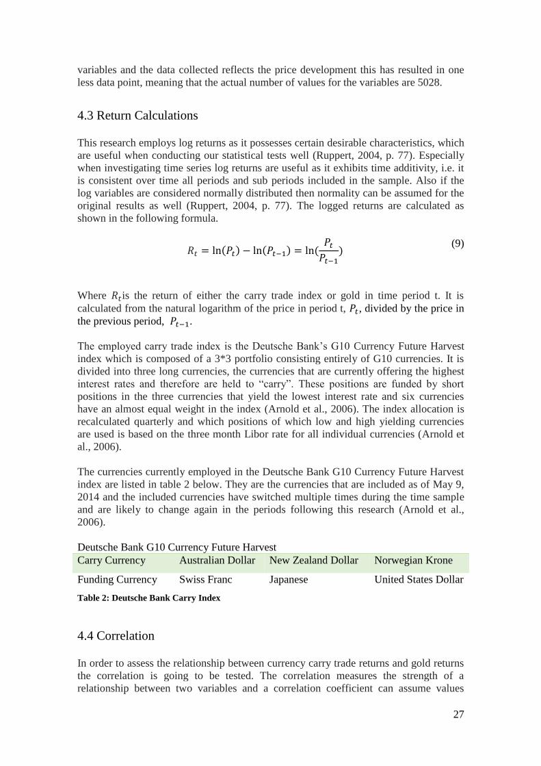
27

variables and the data collected reflects the price development this has resulted in one

less data point, meaning that the actual number of values for the variables are 5028.

4.3 Return Calculations

This research employs log returns as it possesses certain desirable characteristics, which

are useful when conducting our statistical tests well (Ruppert, 2004, p. 77). Especially

when investigating time series log returns are useful as it exhibits time additivity, i.e. it

is consistent over time all periods and sub periods included in the sample. Also if the

log variables are considered normally distributed then normality can be assumed for the

original results as well (Ruppert, 2004, p. 77). The logged returns are calculated as

shown in the following formula.

( ) ( ) (

)

(9)

Where is the return of either the carry trade index or gold in time period t. It is

calculated from the natural logarithm of the price in period t, , divided by the price in

the previous period, .

The employed carry trade index is the Deutsche Bank’s G10 Currency Future Harvest

index which is composed of a 3*3 portfolio consisting entirely of G10 currencies. It is

divided into three long currencies, the currencies that are currently offering the highest

interest rates and therefore are held to “carry”. These positions are funded by short

positions in the three currencies that yield the lowest interest rate and six currencies

have an almost equal weight in the index (Arnold et al., 2006). The index allocation is

recalculated quarterly and which positions of which low and high yielding currencies

are used is based on the three month Libor rate for all individual currencies (Arnold et

al., 2006).

The currencies currently employed in the Deutsche Bank G10 Currency Future Harvest

index are listed in table 2 below. They are the currencies that are included as of May 9,

2014 and the included currencies have switched multiple times during the time sample

and are likely to change again in the periods following this research (Arnold et al.,

2006).

Deutsche Bank G10 Currency Future Harvest

Carry Currency Australian Dollar New Zealand Dollar Norwegian Krone

Funding Currency Swiss Franc Japanese United States Dollar

Table 2: Deutsche Bank Carry Index

4.4 Correlation

In order to assess the relationship between currency carry trade returns and gold returns

the correlation is going to be tested. The correlation measures the strength of a

relationship between two variables and a correlation coefficient can assume values

28

within the range of 1 to -1 (Moore et al., 2008, p. 113). A correlation coefficient of 0

indicates no relationship and the closer the coefficient is to 1 or -1 the stronger the

correlation relationship (Moore et al., 2008, p. 113). It should be noted that correlation

does not measure nor test causality among the included variables but rather provides an

indication of whether the variables tend to vary similarly or not (Moore et al., 2008. p.

143). The findings of correlation statistics must therefore be considered with this in

mind and conclusions derived from these kinds of tests needs to be modest and

consistent with the results.

In this research the returns of our carry trade portfolio are going to be put through the

Pearson product-moment correlation test if the data is found to be consistent with the

assumption behind the test, if not another test needs to be employed with better fit the

data distribution such as the Spearman’s rank correlation coefficient. The Pearson test

requires the data to be measured on an interval or ratio basis and also assumes normality

among the data, something that needs to be tested for (Lund & Lund, 2013). It is also

necessary to have homoscedasticity in the data distribution a (Studenmund, 2006, p.

347). As it tests for a linear relationship between the variables it is also crucial that the

underlying relationship is in fact a linear one as Pearson might not be able to detect a

nonlinear correlation (Lund & Lund, 2013).

If the data distribution does not fulfill the required imposed by the Pearson test another

test will be conducted as earlier mentioned, this as the Spearman test does not have

quite as strict requirements. It does for instance not require a normal distribution nor

does the relationship need to be linear (Hauke & Kossowsku, 2011, p. 92).

4.5 Spillover Effects

In this research we test for the presence of any spillover effects between the carry trade

returns and gold returns, both in terms of the actual returns and the volatility of returns.

This is done with two different statistical tests which are presented in the following

sections as well as the assumptions underlying the tests and the requirements on the

distribution of the data that is imposed by the employed tests.

As the relationship that is being researched tests for effects between returns and

volatility of previous periods on the return and volatility of the current period an

appropriate lag length has to be chosen. Lag length regards to how many previous

variables are included to explain the current outcome (Liew, Khim-Sen 2004, p. 1). An

inappropriate lag length could either lead to missing serial correlation detectable at

larger lag lengths or an excessively large lag length is chosen might produce low power

and unreliable results in statistical tests (Harvey, 1981, cited in Li & Giles, 2013, p. 16).

Several criteria has been developed to find an appropriate lag length which will be

investigated in this research, where a special focus will be put on Akaike’s information

criterion (AIC) as suggested by Liew Khim-Sen (2004, p. 6-7) and Karolyi (1995, p.

17). This will need to be done individually for both the VAR and BEKK GARCH test

and the chosen lag structure that produces the lowest AIC score is the lag length that

minimizes information loss (Karolyi, 1995, p. 15).

In order to employ the appropriate statistical tests a unit root test has been conducted, as

the possibility to make accurate conclusions based on the findings are deeply impaired

by the presence of a unit root. To test for unit root and stationarity among the variables

29

the Augmented Dickey-Fuller test was used. The Dickey-Fuller and Augmented

Dickey-Fuller tests examines whether the means or variance of time series shifts over

time, as it does if the data has a unit root problem. It does so by testing the null

hypothesis of a unit root presence (Elliott et al., 1996, p. 813).

If the properties of the data distribution of a time series shift over time it causes

problems for certain models as the statistical tests used to derive them does not account

for non-stationarity. In such cases more advanced tests are necessary which can include

the developing trends of such data. This does not necessarily implicate that the data

distribution is constant, non-static but rather that shifts in it are not a function of time

(Elliot et al., 1996, p. 817). The stationarity of the included variables must thus be

assessed before conducting the tests that assumes it.

4.5.1 Return Spillover

In order to study a dynamic relationship between several time series the Vector

Autoregression, VAR, has been proposed by multiple researchers due to some different

desirable attributes (Sims, 1980, p. 33; Hansen, 1999, p. 306). It allows the tested

variable in the relationship that is being investigated to depend on both themselves in

previous terms, i.e. lagged, and of other variables in earlier periods, also lagged.

Employing this test does thus show whether, and how much the return in one of our

variables is dependent not only on previous returns of the same variable but also

previous returns of another return, thus the spillover effect between returns of several

variables (Li & Giles, 2013, p. 11).

In order to employ the Vector Autoregression test all included time series need to be

stationary, in this theses this implies that stationarity is required among the gold returns

and carry trade returns. If the data series are found to be non-stationary VAR can still be

used to test the interdependence among the variables but further measures has to be

employed to ensure the reliability of the results (Stock & Watson, 2001, p.101-102).

A bivariate VAR model, which is being tested in this thesis, with two lags has the

following equational form:

(

) (

) (

) (

) (

) (

) (

)

(10)

(Stock & Watson, 2001, p. 110)

A VAR(2) model like this implicate that the current value of variable 1 and 2, and

, depends on a constant, and , the value of both variable 1 and 2 for the last two

previous periods with different associated coefficients as well as an error term. π is the

coefficients associated with the lag periods and the different previous values of the two

variables. The error terms is a white noise vector, implicating it is statistically

uncorrelated with the covariance, and has a zero mean (Fessler, 1998, p. 4).

Equation 10 above can also be described individually for the two variables and the

effects between them and does then follow the equations presented below.

30

(11)

(12)

(Stock & Watson, 2001, p. 110)

The VAR model has the advantage of being able to detect co-movements over other

univariate and bivariate models as it investigates current and lagged variables. This

allows for a more thorough investigation for the relationship between two variables

(Stock & Watson, 2001, p. 110). This benefit is crucial for this research and the reason

VAR has been employed in this thesis.

4.5.2 Volatility Spillover

In order to test for a relationship for any spillover effects in the relationship between

gold and carry trades returns a GARCH, General Autoregressive Conditional

Heteroscedasticity, model will be used. This is an extension proposed by Bollerslev

(1986) of the original ARCH model made by Engle in 1982 (Bollerslev, 1986, p. 307).

It is improved by allowing the model to include less strictly defined lags and provides a

better fit than its predecessor (Bollerslev, 1986, p. 308).

However some further extensions are required for the model to properly suit the data

and research conducted in this thesis. As the relationship between the two variables is

investigated for an effect of conditional variance the test that is to be conducted is

bivariate, this require certain additions when modelling the relationship (Bollerslev,

1986, p. 318). The extension from univariate GARCH analysis to a multivariate one

poses additional problems as the model has difficulties estimating covariances due to

the nonlinearity and nonconvexity in the relationship (Altay-Salih et al., 2003, p. 486).

These problems are addressed in development of the model into the VECH GARCH

which was developed by Bollerslev (1988, p. 318). The VECH GARCH model assumed

constant covariance which is not perfectly accurate but help ensuring that the

multivariate model actually could be solved (Altay-Salih et al., 2003, p. 486). Altay-

Salih et al. (2003, p. 486) described this approach as a tradeoff between the practical

ability and theoretical accuracy of the model.

The development and additions to these models has culminated in the BEKK GARCH

model which in contrast to the VECH GARCH model significantly reduces the number

of included parameters to a much more manageable amount, this is accurate both for

diagonal and scalar BEKK GARCH models (Li & Giles, 2013, p. 13). The BEKK

GARCH approach was introduced by Engle & Kroner (1995) and was extended to

detect specification errors later in 1998 (Kroner & Ng, 1998, p. 817). The basic of the

BEKK GARCH model is presented in the equation below (Kroner & Ng, 1998, p. 820).

31

[

]

[

] [

]

[

]

[

]

(13)

(Kroner & Ng, 1998, p. 820)

Equation 13 represents the structure that is underlying the BEKK GARCH model. in

the equation above is a matrix of the conditional variance between the, in the bivariate

case, two investigated variables at time period t and represent a matrix of constants

(Engle & Kroner, 1995, p. 128). The last, lower, part of the equation is the GARCH

term, associated with , and the matrix captures the ARCH term. As represent the

conditional variance the matrix and GARCH term shows how present conditional

variance between the included variance depends on the conditional variance in the

previous term. Similarly the ARCH term and matrix show the dependence of

conditional variance in time period t on the observed error term for the variables of the

period before t (Engle & Kroner, 1995, p. 128-130).

Reconstructed to equational form the diagonal BEKK GARCH model takes the

following expressions shown in equation 14-16 assuming ARCH and GARCH terms of

only the first order (Kroner & Ng, 1998, 817).

(14)

(15)

(16)

(Kroner & Ng, 1998, 817)

In contrast to other statistical tests used in this thesis the BEKK GARCH statistics will

not be conducted using the statistical software Stata 12 but rather Eviews 7. This is due

to the fact that Stata is not able to run this specific extension of the GARCH model

while Eviews is. The choice of which statistical software is appropriate to utilize has

been based on the article by Brooks et al. (2003, p. 8).

4.6 OLS Regression

The regression analysis is a statistical method that is explaining a dependent variable as

a function of movements in the independent variable(s). The output of the regression

will generate a single equation that will model this relationship between the variables

(Studenmund, 2006, p. 6). It is considered a suitable investigation tool when trying to

look at potential cause and effect relationship (Studenmund, 2006, p. 7). Equation 17

illustrates an example of a multivariate linear regression equation for a time series:

(17)

32

(Studenmund, 2006, p. 15)

In this equation Y represents the dependent variables and X is the independent

variables. Where i = means the ith observation of the respective independent variable.

is the intercept or constant which represents the value of Y if the independent

variables are zero. The other represents the coefficient for the respective

independent variable. The last term in the equation is a stochastic error term, this

variable represents variation that is caused in the dependent variable that cannot be

explained by any of the independent variables. This error term is then made of variation

that can be caused from omitted variables, measurement error, incorrect functional form

or purely random unpredictable occurrences (Studenmund, 2006, 8-13).

The model regression model in this paper is the ordinary least square (OLS) regression

analysis. In order for OLS to be the most appropriate regression equation to use there is

some classical assumptions that must hold for the specific equation for it to be the best

estimator available for regression models (Studenmund, 2006, p. 88).

These assumptions are:

I. The regression model is linear, is correctly specified, and has an additive

error term.

II. The error term has zero population mean.

III. All explanatory variables are uncorrelated with the error term.

IV. Observations of the error term are uncorrelated with each other (serial

correlation).

V. The error term has constant variance (no heteroscedasticity).

VI. No independent variable is a perfect linear function of any other explanatory

variable(s) (no perfect multicollinearity).

VII. The error term is normally distributed (optional assumption).

(Studenmund, 2006, p. 89)

So in order for us in this research to make sure that our estimated regression model is

appropriate we will have to test this model for these assumptions.

For assumption four the test we are going to use is the Durbin-Watson d statistic which

test for if we have positive, negative or no serial correlation (Studenmund, 2006, p.

393). For assumption five the test we are going to use Stata hettest and imtest which

will check the variance of the error term. For assumption three and six we can make use

of a simple Pearson correlation test to check make sure this assumption is not violated

(Studenmund, 2006, p. 393). If we would have any issue with our model we will have to

use alternative regression methods that will help correct for this potential violation.

is the output value in the regression analysis that describes the overall fit of the

estimated model (Studenmund, 2006, p. 50). For hypothesis testing there are two

different tests, the T-test which is for individual coefficients in the regression model

33

(Studenmund, 2006, p. 121) and the F-test is for the overall significance of the model

(Studenmund, 2006, p. 154).

The model we are going to use in order to analyze if gold’s relationship to currency

carry trade have any safe-haven or hedge properties are based on the model from Baur

& Lucey (2010). In the article they investigate these properties in relation to stocks and

bonds applying this model for currency carry trades would then become:

( ) ( )

( )

(18)

The model is then constructed in the way that we test if the gold returns dependency on

the carry trade returns. In order to account for differences in the relationship in turbulent

and extreme market conditions we have constructed dummy variables for different

quantile thresholds. represents the dummy variables for different quantile levels of

the carry trade returns. We choose the quantile levels to be 1%, 5% and 10% as we

believe these are appropriate to capture these different market states. As Baur & Lucey

states ”the choice of the quantiles is arbitrary to some degree” (Baur & Lucey, 2010, p.

220). If the carry trade returns are larger than the q% the value of the dummy variable

will be zero and one if not.

We will also test this relationship for lagged periods were we test the current periods

gold returns against previous period(s) carry trades return to make sure of the nature of

the relationship. Since we have not found any earlier paper that have investigated the

relationship between gold and carry trades.

This regression will help us extend on Clarida et al. (2009, p. 20) findings and

investigate if gold can help to offset the high negative returns for carry trades during

high volatility states.

We explained the properties of safe-haven, hedge and diversifier in the theoretical

framework which together with the results from the regression will be our basis to

analyze this.

4.7 Hypotheses

Seeking to answer the research question stated in chapter one, we constructed the

following hypotheses. The hypotheses are divided into subgroups below regarding the

different tests they correspond to. Following up on and concluding the answers to the

various hypotheses will be done in chapter 6 after the empirical findings have been

presented. The adopted confidence level for all hypotheses testing in this thesis is 95%

which indicate that if the findings regarding of a found relationship has shown to, using

our data, have a lower chance than five percent to be discovered by chance it will be

deemed to be correct and the relationship in question will be concluded as valid. More

specifically if the significance level found during the testing exceed the critical value of

95% the null hypothesis that no relationship can be concluded will be rejected in favor

of an alternative one of an existing relationship.

34

4.7.1 Correlation Testing

Hypothesis 1: During the correlation testing between gold returns and carry trade index

returns the hypothesis that will be tested is whether there is any correlation relationship

between the two variables shown in the following expressions:

4.7.2 Spillover Effects

Hypothesis 2 & 3: This hypothesis concerns the testing of mean spillover effects using

the VAR model and will thus conclude whether the current returns of either are

influenced by the past returns of the other variable. This is presented in two hypotheses

to differentiate between the two variables.

Hypothesis 4: As the diagonal BEKK GARCH test will not be able to deduct neither

direction nor causality of the included variables this hypothesis will only concern if

there is any volatility spillover effect between the variables at all.

4.7.3 Regression Testing

Hypothesis 5: The regression is testing whether the relationship between gold returns

are, in relation to carry trade returns, exhibiting hedge or safe haven characteristics and

is tested as such. The hypothesis is thus constructed in order to test for these

characteristics.

35

5. Empirical Findings This chapter display what has been found using the data and methods presented in the

previous chapter. Firstly it provides background information regarding the data to

provide some understanding and familiarity to the data employed. Sequentially the

output of the different statistical test and measures are presented which in following

chapters will be analyzed and discussed.

5.1 Descriptive Statistics

The data employed in this research is explored and presented in the following section as

well as some overall traits and characteristics. The development of the time series and

the statistical properties associated with it are as well included to provide an overview

on the data from which inferences in later sections are made.

5.1.1 Development

The following graph in figure 3 shows the development of the investigated variables in

the chosen time period. It is based on the raw data collected from Thomson Reuter

Datastream and Deutsche bank. As can be told from the graph investors holding either

gold or following the currency carry trades index has over these 20 years experienced

substantial positive returns. The gold price has been indexed to 100 at the start of the

time horizon to facilitate comparison.

Figure 3: Gold & Carry Trade Development

Source: The authors

Interestingly what can also be told from the graph is that the development of the two

different variables does not seem to follow any similar pattern. Carry trades have

experienced systematically large increases evenly distributed over the time horizon with

the exception of a large dip in around the end of 2008 to the beginning of 2009.

0

100

200

300

400

500

600

700

Development 1993-2013

Carry Index Gold Index

36

Whereas the gold price development in was almost stagnant for the first half which was

followed by an exponential increase in the latter.

The development over time is also summarized in the following table which shows the

total development in the entire sample as well as the average annual. The returns

presented in table 3 below are however simple returns and not the log returns that have

been put to use in the statistical tests. This should be kept in and the returns presented

below rather provide some basic info surrounding the development over time and

conclusion will not be drawn from these returns.

Total Return Avg. annual return

G10 Currency Future Harvest Index 449,08% 8,89%

Gold Price 385,90% 6,99% Table 3: Total Returns

5.1.2 Return Distributions

As can be derived from table 4 the two investigated variables do not differ only in actual

returns but also significantly in the return distribution.

Observations Mean Min Max St. Dev

Gold returns 5028 0,00031 -0,0628 .07382 .0103

Carry trade returns 5028 0,00034 -0,0801 .06072 .0065 Table 4: Descriptive Statistics

Table 4 contains the information of the return distribution of daily returns regarding the

entire time horizon.

Figure 4: Gold Return Volatility

Source: The authors

Figure 4 and 5 depicts the volatility of the gold and carry trade returns over the time

period of 1993 to 2013. What can be said generally is that over the entire time horizon

-0,08

-0,06

-0,04

-0,02

0

0,02

0,04

0,06

0,08

0,1

Gold Returns

Gold Returns

37

that the volatility is generally higher for the gold returns than the carry trade return. This

is also reaffirmed from table 4 above as the standard deviation of the gold returns are

higher than those of the currency carry trade index, 0,0102829 compared to 0,0064897

respectively.

It seems that the returns of carry trade has experienced a more stable growth over time

rather than the gold which for the larger part of the sample has not shown a significant

positive return but only in later years shown substantial increase in value, as can be seen

in figure 3 as well. This kind of development is more unpredictable and, to the extent

that risk is measured by volatility more risky.

Figure 5: Carry Returns Volatility

Source: The authors

The currency carry trade returns volatility on the other hand as is depicted in figure 5

shows a much smaller distribution in how the returns are distributed. It does though also

show a much larger downside risk as individual observations of losses are much larger

than were found among the gold returns.

What also can be said by looking at figure 5 is that the carry trade returns experienced a

long period of tranquility between late 90s and mid 2000s. This was followed by an

unsettled period which also is depicted in figure 5 before. During and after the financial

crisis period the returns of the carry trade index have been highly volatile with

comparatively high positive gains followed by even larger losses following days.

Still, the volatility of gold returns is also greater during this period and although the

carry trades have some more extreme losses in their observation the gold returns

volatility still substantially exceed that of the carry trade index over the entire time

sample.

-0,1

-0,08

-0,06

-0,04

-0,02

0

0,02

0,04

0,06

0,08

Carry Trade Returns

Carry Returns

38

5.2 Correlation

In order to figure out which correlation test to conduct the normality of the data has to

be assessed as described in chapter 4. This is done graphically, looking at the histogram

and q-q and p-p plots of the return variables, and statistically by conducting the Shapiro-

Francia. The histograms and plots are presented in appendix 1. The Shapiro-Francia

test was used as the number of observations exceed 2000 making Shapiro-Wilks test for

normality inappropriate. The result of the Shapiro-Francia test is shown in table 5

below.

Variable Obs W’ V’ z Prob>|z|

Gold Returns 5028 0,9209 232,362 13,805 0,00001

Carry Return 5028 0,8734 371,869 14,997 0,00001 Table 5: Normality Test

As the Shapiro-Francia test for normal data tests for the null hypothesis that the data is

normally distributed it can be rejected at the chosen 95% confidence interval and from

this test the inference can be drawn that the data in not normally distributed.

Looking at the graphics provided in appendix 1 the findings regarding normality is

reaffirmed and for both return variables included in the research it can be concluded that

neither exhibits a normal distribution. As for the correlation testing this implicates that

the Pearson product-moment correlation is inappropriate as it requires normal

distribution among the investigated variables. It is thus appropriate to conduct the

Spearman correlation test instead of Pearson as the latter also only detects linear

relationship and deriving whether the underlying relationship is actually linear or not

would require further investigation.

Due to the reasoning previously presented the Spearman rank correlation coefficient test

was conducted and the result is presented in table 6 below.

Spearman’s ρ Prob > | | 0,0949 0,000 Table 6: Spearman's Correlation

The probability variable of 0,000 means that the null hypothesis that the returns of gold

and the carry trade index returns are independent of each other can be rejected and the

correlation coefficient of this test is statistically significant. The Spearman’s rho, ρ,

represents the correlation coefficient of the test and although significant assumes the

low value of 0,0949.

This correlation test is conducted over the entire period of 20 years, including all 5028

observations. Since the correlation coefficient is significant and assumes a positive

value this indicates a positive relationship between the returns of gold and carry trade,

i.e. generally if the gold returns are positive it is associated with positive returns of the

carry trade index. Although this relationship is only to a certain limited extent as the

value of the correlation coefficient is relatively low.

39

5.3 Spillover Effect

Before conducting the various spillover test the presence of a unit root problem among

the data sample has to be assessed as described in chapter 4. The augmented Dickey-

Fuller was conducted to test for stationarity and the output is presented below in table 7.

The augmented Dickey-Fuller test checks the null hypothesis that there is a unit root

among the data, i.e. that the data distribution is non-stationary.

Test

Statistic

1% Crit.

Value

5% Crit.

Value

10% Crit.

Value

P-value

Gold Z(t) -70,820 -3,430 -2,860 -2,570 0,000

Carry Z(t) -72,578 -3,430 -2,860 -2,570 0,000 Table 7: Unit Root Test

Investigated at the 1%, 5% and 10% critical values both for the gold returns variable

and the currency carry index return variable, both are found to have a Z(t) value well

above that required for even the 1% critical value. Thus, the null hypothesis can be

rejected for both variables and we can conclude that the data is stationary. Without the

presence of a unit root and the problems that would entail the previous suggested tests

can be employed without further extensions or additions.

5.3.1 Mean Spillover

With stationarity assured the appropriate lag length has to be derived which was done

using the Akaike information criterion. The optimal number lag structure is the one

producing the lowest AIC score and the scores for various lag lengths are presented in

appendix 2. As is shown from the table in appendix 2 the VAR model was tested for up

to 15 lags and the amount of lags that produced the best model following the AIC was

employing 12 lags. Thus 12 lags are used to derive the mean spillover effects between

the two variables.

The values denoted with a * are the lowest AIC values produced in each individual test.

Derived from the appendix 2 above can be said that the appriopriate lag structure that

will ensure the lowest information loss. Thus when conducting the VAR test a lag

length of 12 lags will be adopted. Adapting equation 10 from chapter 4 to include

twelve lags it will take the following look:

(

) (

) (

) (

) (

) (

) (

)

(19)

In table 8 and 9 below the output from the Vector Autoregression is displayed.

40

Gold Ret. Coef. z P>|z| Coef. z P>|z|

Gold Ret.

Carry Ret.

L1 0,0003 0,02 0,983 0,0756* 3,36 0,001

L2 0,0059 0,42 0,676 -0,0616* -2,73 0,006

L3 0,0095 0,67 0,502 0,0351 1,56 0,119

L4 0,0153 1,09 0,278 -0,0373 -1,66 0,097

L5 0,0102 0,72 0,471 -0,0069 -0,31 0,757

L6 -0,0419* -2,97 0,003 0,0143 0,64 0,525

L7 -0,0049 -0,35 0,727 -0,0185 -0,82 0,41

L8 -0,0085 -0,6 0,547 -0,0406 -1,81 0,071

L9 0,0370 2,61 0,009 0,0016 0,07 0,942

L10 -0,0178 -1,25 0,209 -0,0592* -2,64 0,008

L11 -0,0127 -1,1 0,270 0,0900* 4,01 0,000

L12 -0,0257 -1,82 0,069 0,0486 2,16 0,031 Table 8: VAR Gold Returns

Coefficient values denoted with a * are statistically significant at a 95% confidence

interval. Expreseed individually for the Gold return variable the VAR-model take the

following form before plugging in the values from table 8.

(20)

is the return of gold in time period t.

Inserting the values from table 8, although keeping in mind that only the constant

proved statistically significant at the chosen 95% confidence interval, produces the

following expression for the mean spillover from carry trade returns on gold returns:

(21)

41

Carry Ret. Coef. z P>|z| Coef. z P>|z|

Gold Ret. Carry Ret.

L1 0,0198* 2,22 0,027 -0,0300* -2,12 0,034

L2 0,0139 1,56 0,118 -0,0109 -0,77 0,443

L3 -0,0052 -0,58 0,562 -0,0267 -1,88 0,060

L4 -0,0168 -1,88 0,060 0,0119 0,84 0,401

L5 0,0037 0,41 0,681 -0,0611* -4,31 0,000

L6 0,0279 3,13 0,002 -0,0146 -1,03 0,303

L7 -0,0134 -1,5 0,134 0,0041 0,29 0,773

L8 -0,0278* -3,12 0,002 -0,0194 -1,37 0,171

L9 -0,0124 -1,39 0,166 0,0220 1,55 0,121

L10 -0,0224* -2,51 0,012 0,0107 0,76 0,448

L11 -0,0088 -0,99 0,322 0,0232 1,64 0,101

L12 -0,0206* -2,31 0,021 0,0399* 2,82 0,005

Table 9: VAR Carry Returns

Again all coefficient that have been found to be statistically significant have been

marked with a *,

(22)

is the currency carry tradew return of period t. Deriving the VAR model for testing

the mean spillover effects on the carry trade returns shows that also here most

parameters have not been found to be statistically significant ona 95% confidence level.

In addition the intercept, , which were found to be significant also for the gold return

equation. Using the coefficients produced by the VAR test produce the following

expression:

(23)

5.3.2 Volatility Spillover

Before conducting the BEKK GARCH test the order of the ARCH and GARCH term

has to be determined which is done similarly to the lag structure in the VAR model.

Minimizing the Akaiko information criterion is desirable as lower AIC scores are

associated with less information loss. The following matrix in table 10 shows the AIC

score for different ARCH and GARCH orders.

42

1 2 3 4

1 -14,3304 -14,3369 -14,3361 -14,3353

2 -14,3363 -14,3317 -14,3379 -14,3371

3 -14,3360 -14,3386* -14,3305 -14,3371

4 -14,3352 -14,3378 -14,3373 -14,3288 Table 10: GARCH Lag Test

As can be told from table 10 the lowest AIC-score is produced by the diagonal BEKK

GARCH model with two ARCH and three GARCH terms. This model can alo be

expressed BEKK GARCH(2,3). With a ARCH order of two and GARCH order of three

the model deemed appropriate for our data includes two autoregressive lags and three

moving average lags.

Since the two terms measure the impact of different factors on current conditional

variance there is no issue in adopted different lag structures for them. It could be, as in

this case, appropriate to use a certain lag length of autoregressive lags and another for

moving average lags to better model the relationship of conditional variance between

the two variables.

The result from running a diagonal BEKK GARCH(2,3) is presented in the following

table and the different parameters will be noted again as the model showing the tested

relationship are matched with the values produced by the test.

BEKK GARCH Coefficient Denotation

M11 5,79E-07** M22 6,70E-07** M12 0,0005** A1, 11 0,2717**

A1, 22 0,2746**

A2, 11 -0,0248

A2, 22 0,2614**

B1, 11 0,6023**

B1, 22 0,5927**

B2, 11 0,5822**

B2, 22 0,5428*

B3, 11 0,4700**

B3, 22 0,4423** Table 11: BEKK GARCH Test

The statistically significant parameters from the diagonal BEKK GARCH test hve been

denoted with a *. Whether one or two * is used represents whether the finding is

significant on a 95% and 99% confidence interval respectively.

Applying these coefficients into the equational form of the model earlier presented in

equations 14-16, chapter 4 and surpressing the error term gives us the following:

43

(24)

(25)

(26)

What can be derived from table 11 is that most effects from autoregressive and moving

average lags have a relationship on the conditional variance at time period t, with the

exception of A2,11 which on the other hand is the only coefficient not found to be

statistically significant.

As it is difficult to make any inferences about parameters that are not statistically

significant the parameter A2,11 will be kept in special regard. With a coefficient of

0,024761 and a standard error of 0,026989 not much can be concluded regarding the

relationship, barely even the direction of it as it centers on 0.

We also note that the effect of the various B-parameters are without exception greater

than those coefficient values of A-parameters indicating that for the model produced by

the BEKK GARCH test, the GARCH effect is substantially greater than the ARCH

effect. The implication of which is that previous conditional variance has a greater

magnitude in determining the conditional variance of the current period than the squared

residuals do.

The general finding from this test is that conditional variance and in extension volatility

is positively related to lagged residuals and of conditional volatility in previous periods.

This is valid for almost all parameters and the included 2 autoregressive lags and 3

moving average lags.

This result is illustrated in the figure 6 below which maps the respective variance of the

two investigated variables over the entire time sample as well as their covariance. The

covariance between the two fluctuate around zero for most of the time sample and is

only shifting substantially from that in periods where one or both of the variables

experience a high level of distress.

44

Figure 6: Return Variance

Source: The authors

This graph also demonstrates how gold over most period in the time sample have

experienced higher levels of volatility. Interestingly a volatility spike in one of the

variables is usually not accompanied by especially large increases, if any at all, in the

variance of the other variable. Even when this is not the case as in 2008-2009 and

around 2012 where the volatility for both gold return and carry trade returns experiences

a surge at the same time the drops in the covariance indicate that the variables do not

move in the same direction, rather the opposite.

5.4 Regression

Gold returns Coefficient Standard Error p>|T|

Carry trade returns 0,1835 0,0518 0,000

Carry trade returns (10%) 0,0003 0,0033 0,075

Carry trade returns (5%) -0,0007 0,0012 0,579

Carry trade returns (1%) 0,0059 0,0009 0,709 Table 12: Regression Analysis

( ) ( )

( )

(27)

Table 12 shows the results from our regression analysis of the safe-haven, hedge and

diversifier characteristics of gold for carry trades.

The regression model have been tested for the assumptions discussed in chapter 4. The

vif test for multicollinearity showed a value of 2,01 which is within the acceptable

-0,0002

-0,0001

0

0,0001

0,0002

0,0003

0,0004

0,0005

0,0006

0,0007

0,0008

0,0009

Return Variance

Gold Var

Carry Var

Covar

45

range. If the vif value is over 5 one can start to consider multicollinearity as an issue

(Studenmund, 2006, p. 259).

Due to the nature over our data with the long time series covering both normal and

turbulent market environment, it is likely that the model will experience

heteroscedasticity with a non-constant volatility. After conducting the White-test in

Stata we found that this was the case. Since that is an issue of the nature of the data the

heteroscedasticity is likely of the pure form which will not cause bias in the coefficient

estimates. It will create some bias for the T-values which would generate unreliable

hypothesis testing (Studenmund, 2006, p. 352-354). In order to fix for this we run the

regression with heteroscedasticity corrected standard errors which will correct the

standard errors of the models and generate t-values that is without inference from the

heteroscedasticity enabling the model to be used for hypothesis testing (Studenmund,

2006, p. 365-366).

Table 12 shows the final results from the regression model with heteroscedasticity

corrected standard errors. The lagged variables have been excluded from the table 12

since all of them was statistically insignificant. The only statistically significant

relationship that was found was between Carry trade returns and gold returns within the

same time period. The coefficient of 0,1834639 indicates that relationship some a low

level of average correlation. This means that for a 1% change in the carry trade returns

would yield an increase of 0,1834639% in the gold returns. This then demonstrate a

positive co-movement between the assets.

Since the quantiles of 1%, 5% and 10% showed insignificant we cannot determine the

relationship between gold returns and carry trade returns in different volatility states.

5.5 Portfolio Simulation

Figure 7: Portfolio Simulation

Source: The authors

0

100

200

300

400

500

600

Carry Trade Portfolio vs Carry Trade Portfolio with Gold

Portfolio with gold Carry trade portfolio

46

Time period 1993-2012 Carry trade portfolio Carry trade portfolio with gold

Average annual return 8,54% 8,41%

Annual standard deviation 10,30% 9,137%

Average annual sharpe ratio 0,5447 0,6008

% Carry Trade 100% 80%

% Gold 0% 20% Table 13: Portfolio Simulation

The table and graph above illustrates a portfolio simulation over our sample period of

March 151993 to March 12 in 2013. The comparison includes one portfolio which

consists of 80% Carry trade and 20% gold and the other is a full carry trade portfolio.

This simulation shows that including gold in the carry trade portfolio reduces the

standard deviation and gives an increase in the risk/return trade-off given by the Sharpe

ratio. We can see from the graph that the full carry trade portfolio outperforms the one

with gold up until around the financial crisis were the drop is substantially larger for the

full carry trade portfolio. The full carry trade portfolio outperforms the gold portfolio

over the time period, however this comes at a cost of a high risk. Looking at the Sharpe

ratio over the whole time period including gold in the portfolio will give you a higher

payoff given the risk undertaken.

5.6 Hypotheses Testing

In light of the empirical findings presented in this chapter the hypotheses which

concluded the previous chapter will be revisited. By looking at the results we will be

able to conclude what relationships have been found between gold returns and carry

trade returns. The various hypotheses and the rejection and acceptance of which will be

assessed in further depth in the following chapter as this part only looks at what can be

immediately derived from the empirical findings.

Hypothesis 1: Correlation

Looking at table 6 in which the result from the Spearman correlation test is shown it can

be said that there is in fact some correlation present between these two variables.

Although a correlation coefficient of only 0,0949 it is statistically significant not only

on the chosen 95% confidence interval but even on a 99% confidence interval as well.

Thus is can be concluded that there is a small positive correlation between the returns of

gold and of the carry trade, i.e. hypothesis 1 of no correlation can be rejected.

47

Hypotheses 2 & 3: Mean Spillover

Section 5.3.1 in this chapter regarding the mean spillover effects did not produce many

significant variables, see table 8 and 9. Although one lagged significant variable it

would be enough to reject either of the hypotheses 3 and 4 if it would be for for the

return equation of the other variable. Derived from table 8 where the returns of gold is

being testing, statistically significant coefficients were discovered for the lagged trade

return of carry trade for lag 1, 2, 10, 11 and 12. This implicate that gold returns has a

relationship with the lags of carry trade and hypothesis 2 of no mean spillover from

carry trade to gold returns can be rejected.

Similarly for carry trades returns, some lags of gold returns were found to be

significant. As seen on table 9 these were lags 1, 6, 8, 10, 12.As the returns of the

currency carry trade index exhibit a relationship with the lagged return on gold

hypothesis 3 can also be rejected on a 95% confidence interval.

Hypotheses 2 and 3 are both rejected as the empirical findings show that there is mean

spillover effects between gold returns and that of carry trade.

Hypothesis 4: Volatility Spillover

The BEKK GARCH Model derived from the values in table 11 and expressed in

equations 24-26 including significant ARCH and GARCH terms implicate that to it

some extent manage to explain the conditional variance in the present period. As this

model cannot show the direction of volatility spillover but rather just conclude the

presence of any such effect. As earlier mentioned the model showed significance for

almost all included parameters so we can deduct that there is a spillover effect in

variance between gold and carry trade returns. Hypothesis 4 is rejected.

Hypothesis 5: Hedge and Safe Haven Characteristics

48

Since the results that most of the variables in the regression analysis showed to be

insignificant we cannot reject the null hypothesis. Meaning that we did not find

statistically significant evidence from the regression if gold have safe-haven

characteristics or not. Regarding hedge we can see that the average correlation between

the carry returns and gold are positive but far from 1, which indicates that it experiences

diversifier characteristics rather than hedge characteristics, where average correlation

should be non-positive or negative.

49

6. Discussion This chapter connects the empirical findings and the hypothesis testing in the previous

chapter with theories and previous research. It makes conclusion regarding the findings

and the implications that are derived from it. Further what the empirical findings

indicate in practice as well as theoretically is discussed and concluded and a general

overview of the results finishes the chapter.

6.1 Summary Results

What was actually discovered in the last chapter is briefly reintroduced here as to

remind from where the discussion takes off and provide a distinction between the

empirical findings and discussion.

Firstly, a significant correlation between gold returns and carry trade returns was

discovered and it indicated a positive relationship which means that the two variables

tend to vary in the same direction. But the correlation coefficient exhibits a small value

and the closer it is to zero the weaker this relationship. Thus with the relatively low

correlation the returns do not vary much in the same direction.

Secondly, significant findings were also found regarding the existence of mean spillover

effects on returns between the two variables. This was found for both variables

individually, meaning that carry trade returns has mean spillover effect on gold returns

and vice versa. The dispersion between the effects these variables had on each other

differed slightly and not much can be said regarding the direction of the relationship.

The twelve included lags in the model were dispersed relatively arbitrarily for the carry

trade return mean spillover effects on gold return. Regarding the gold return spillover

effects on carry trade returns there is an indication that later lags, 7-12, tend to have a

negative relationship whereas earlier lags differ between each different lag.

Thirdly, there were significant findings regarding the volatility spillover effects as well

indicating that there are in fact volatility spillover effects between gold returns and carry

trade returns. Due to the limitations of the employed diagonal BEKK GARCH test not

much can be derived regarding the nature of the relationship, rather it implicates that

there is one. This means that the volatility of at least one of the return variables have

spillover effects on the volatility of the other, this could due a one-way or two-way

relationship which is impossible to conclude from this result. However the finding show

that this effect has to be taken into special consideration when contemplating

undertaking positions in both the underlying assets.

Fourthly, the regression testing the hedge and safe haven characteristics did not manage

to found neither hedge or safe haven characteristics for gold on carry trade returns. Non-

surprisingly however it found that for the chosen confidence interval there are

diversification benefits of combining gold and a carry trade strategy in a portfolio. But

for the extreme observations in the 1, 5 and 10% quantiles the observed relationship was

not found statistically significant so we cannot conclude whether gold works as a safe

haven or hedge for carry trade or not.

50

6.2 Carry-trade and Gold Correlation

Carry trades have mostly been researched in isolation to uncover its’ various

characteristics but investors has seldom taken only a position in currency carry trades

but rather holds an entire portfolio of numerous different assets and asset classes. As

this is the case some recent literature has focused on carry trade as a specific asset class

to include in a portfolio of others which is where this research draws ground as well

(Das et al., 2013). Extending the understanding of how the returns of carry trades and

gold leads to a more effective matching of the two different assets when building a

portfolio and following findings regarding this relationship is described as discovered

by this research.

The positive relationship between gold returns and those of the currency carry trade

index that is derived from the positive correlation coefficient produced by the

correlation test means that the two variables vary in the same direction to some extent.

Though since the coefficient value is not higher than 0,0949 the correlation dependence

between the different returns can be questioned. In the case of this research as both

investigated variables have experienced substantial growth over the time period and the

small positive correlation could thus been due to both variables exhibiting positive

returns in the majority of observations. As is the case with correlation tests the actual

dependence and causality of this relationship cannot be concluded.

That gold and carry trade returns only demonstrate a weak correlation, small correlation

coefficient, extend on the conclusion derived by Das et al. (2012, p. 256) who argued

that carry trade strategies only show moderate correlation to equity markets as well. It

also reaffirm the findings of McCown & Zimmer (2006, p. 11) that gold only exhibit

low correlation with other asset classes and extend those asset classes to include

currency carry trade.

As carry trade returns and gold returns possesses a very small positive correlation

coefficient there is definitely diversification benefits attached to including the two in a

portfolio. This finding is also reaffirmed in the regression analysis which found a

positive but low relation between gold and carry trade returns. Combined with attractive

growth over the investigated time period indicates that the two assets are viable

investment strategies and could beneficially be pooled in a portfolio. This is also

illustrated in the portfolio simulation where the portfolio combining gold and the carry

trade strategy offer a higher risk adjusted return, measured by the Sharpe ratio, than the

one consisting of only currency carry trade, 0,6 and 0,56 respectively.

But the relationship between gold returns and returns of carry trade is not quite as

simple as indicated by the correlation testing. Just as Burnside et al. (2011a; 2011b)

argues that the risk profile of carry trades is not appropriately covered by usual risk

factors, special properties of the relationship between gold returns and carry trades also

needs to be considered. This is where the spillover effects between the two become

relevant.

51

6.3 Spillover Effects

With the relationship of the same time period established by testing for the correlation

which discovered low correlation and as both assets over the time period produced

attractive returns an investment strategy combining them would seem like a good idea.

However the effect on the respective variables attributable to the behavior of the other

past behavior of the other variable could be rather drastic effect and substantially affect

the performance of a portfolio including consisting of these two assets.

The result regarding the mean spillover effects are although conclusive enough to

establish that for both gold returns and carry trade returns mean spillover between the

two variables exists. However the findings that the different significant lags produced

different coefficient signs make generalization beyond the point of rejecting the

hypothesis of no spillover effect difficult. This also causes complications when trying to

match the two assets as there is no clear cut relationship. The different signs associated

with the cross-lag dependence between the variables are nonetheless unintuitive as the

VAR test also shows that the relationship between the returns on their own lagged

returns also shifts between positive and negative relationships.

It should be kept in mind that although significant many of the coefficients produced

when testing for mean spillover have small coefficient values, indicating that the

relationship between returns in the current period and of previous returns is relatively

small. These results should thus not be interpreted as explaining nor forecasting actual

returns in a period but rather adding to relationship between gold and carry trades

return.

As the relationship between currency carry trade and the equity markets has been

established (McCown & Zimmerman, 2006, p. 11) and also so the relationship between

equity markets and gold (Katechos, 2011, p. 558) finding spillover effects, albeit small,

in extension between gold and carry trade is not surprising. Thus special caution need to

be considered when combining the assets in a portfolio, but with small spillover effects

on return and most parameters tested, lags, insignificant other factors might be more

crucial in determining the portfolio behavior. That too much emphasize should not be

put on implementing and managing return spillover effects between the two is

reinforced by the portfolio simulation presented in the last chapter as portfolios

consisting of the two assets rather than just one of them has demonstrated higher risk-

adjusted returns all through the implemented time period.

The volatility spillover effects that we were able to conclude in the previous chapter are

a bit more difficult to interpret as the employed diagonal BEKK GARCH model does

not imply direction or causality of the spillover effects. The implication of this which

can also be shown from figure 6 is that periods of high volatility in one of the return

variables is associated with the increased volatility in the other variable as well. To the

extent that volatility is considered as risk the overall risk decreasing benefits of

matching gold and carry trade strategies in a portfolio are somewhat diminishing due to

this effect. It should be told that figure 6 also shows that in the periods of high volatility,

52

when spillover effects should be observable, the covariance between the two variables

has assumed negative values. If this is the case the benefits of combining the two assets

are greater than what is achieved simply from diversification. What can be read into this

is that in moments of high volatility the returns of gold and carry trades generally moves

in opposite directions, this would indicate safe haven characteristics for gold. However

the regression analysis failed to reproduce this finding making inferences about whether

gold can be considered a safe haven for carry trade investments mere speculations.

6.4 Diversification Benefits of Gold

For one of the objectives of our empirical findings was to see to see if gold could be

included in the currency carry trade portfolio in order to help control the downside risk

for high volatility states when currency carry trade experience very negative returns.

The main tool used for this investigation was the regression analysis which showed that

there was no statistical significant relationship between gold returns and carry trade

returns for the more extreme quantiles 1%, 5% and 10%.

From the regression we found that there was a statistical significant relationship

between the gold returns and the currency carry trade returns within the same time

period. From Baur & Lucey’s (2010, p. 219) definition of the different asset

characteristics hedge, diversifier and safe haven introduced in chapter 3, based on our

findings of the relationship between carry trades and gold, gold can be characterized as

a diversifier for the carry trade portfolio. The regression analysis shows that they exhibit

a positive but not perfect correlation. As for a diversifier there is no guarantee that this

correlation property will hold during extreme markets states.

The graph illustration, figure7, the performance of a carry trade portfolio with 20% gold

versus the normal currency carry trade portfolio further support this. The results of this

shows that including the gold in the portfolio increase the average annual Sharpe ratio

from 0,54 to 0,6 over the time period of 15 of mars 1993 to 12 of mars 2013. The

portfolio including gold also have a lower standard deviation showing that there indeed

might exist benefits in diversifying a carry trade portfolio with gold.

Following Markowitz (1959) famous modern portfolio theory introduced in chapter 3.

There is certainly the main concern when it comes to portfolio design to design the

portfolio with respect to the risk/return trade-off. According to this view the addition of

gold in a carry trade portfolio exhibits certain benefits yielding a higher return for the

risk incurred. Gold within the portfolio will give the investor a high risk premium for

holding the portfolio. Our findings have shown that there exists the possibility to reduce

the volatility of the carry trade portfolio with inclusion of gold.

The lowered volatility will be tied to certainly a lower possible payoff, so the central

theoretical issue also in the discussion will be the investors’ preferences and the

behavioral finance aspects. The findings of this study can only show the benefits how

gold can help mitigate some losses and help stabilize the portfolio over time. However

the inclusion of the gold will also lower the potential payoff shown in the portfolio

simulation graph in chapter 5. The full carry trade portfolio outperforms the gold up

until that point when the financial crisis hit. It is then evident that the losses incurred are

53

far greater without gold in the portfolio. Both portfolios do drop substantially in value

during this time. The illustration of the performance differences for the gold price

versus the carry trade portfolio show that during the time of the crisis both the gold and

the currency carry trade portfolio drops. The gold price drops substantially less

compared to the carry index. The graph however is intuitively following the findings of

our empirical research where the gold and carry trades seem to follow a weak positive

correlation. This graph might suggest that this relationship holds even through more

turbulent times, since our statistical test on this proved insignificant we cannot prove

this is the case during 1993-2013.

Lustig & Verdelhan’s (2007) findings of the diversification benefits of the inclusion of

different currencies in the currency portfolio can be extend to our findings. Showing

that there is certainly increased diversification benefits of including more assets in the

portfolio, i.e. gold.

Extending on the current issue of the risk drivers of carry trades there could be so that

the carry trades and gold can share some of these drivers, given the properties of the co-

movements.

54

7. Conclusion & Recommendations In the final chapter of this thesis the research question will be answer, drawing upon

the results presented in the earlier chapters. Then concluding remarks regarding the

entire research and how it was conducted leads to an assessment of the validity and

reliability of the study which were introduced in chapter 3 and various ethical concerns

are also addressed. The thesis is settled with a section of suggestions for further

research.

7.1 Conclusion

The purpose of this research was to investigate the relationship in the movements

between currency carry trade returns and gold returns and also to examine the potential

safe-haven, hedge or diversifier characteristics of gold in relation to currency carry

trades. The sample period was between the 12th of Mars 1993 to the 12th of mars 2013.

The currency carry trade was represented by Deutsche Bank’s G10 Currency Future

Harvest index, and the gold prices were downloaded from the Thomson Reuters

database. Empirically this was investigated through the means of correlation, mean and

volatility spillover and a regression analysis.

The correlation and volatility spillover effects were to determine the relationship and

partly co-movements of the assets. The regression analysis enabled us to look closer to

how this relationship alters in different market states.

Complemented by a portfolio simulation, this test gave evidence for the co-movements

between carry trade returns and the gold returns and clearly established that there is

diversification benefits to attain by matching gold and currency carry trade investments

in a portfolio. This gives answer to the research questions stated in chapter 1:

Is there a co-movement between currency carry trade returns and gold price returns?

According to the empirical test in our study, mainly the correlation test and the

regression analysis. We found that there is a weak correlation between currency carry

trade returns and gold price returns.

Are there any spillover effects between currency carry trade returns and gold price

return?

Our empirical test found that it exists mean spillover effects between currency carry

trade returns and gold price returns. However our significant returns exhibited different

coefficient signs so we cannot draw conclusion beyond the point of the existence of the

mean spillover effects. As for volatility spillovers our results showed their existence.

Due to the nature of the BEKK GARCH test we cannot conclude the direction of the

relationship merely establish its existence.

As sub purpose we wanted to briefly look into the characteristics of gold in a carry trade

portfolio. Given the insignificant results from the regression analysis for the dummy

variables covering the lower quantile returns. We cannot conclude that gold would have

any hedge nor safe-haven properties. However due to the weak correlation found in the

correlation test and in the regression model during our time period gold showed to

55

exhibit diversifying characteristics to a currency carry trade portfolio. Due to the

insignificant results in we cannot conclude anything regarding the relationship during

the higher volatility states.

7.2 Contributions

When we began conducting this research we found that there was a lack of research

investigating the portfolio aspects of currency carry trades. Our findings helps giving

empirical evidence for the benefits of diversification in a currency carry trade portfolio

by including gold. Our conclusions considered together with Lustig & Verdelhan’s

(2007) findings of the diversification benefits of including different currencies can help

pave the way to further explore the portfolio aspects and benefits of currency carry

trades. The results of this research also extends on the empirical evidence discovered by

Das et al. (2013) on if and how carry trades can be effectively implemented in portfolios

consisting of other assets.

From Clarida et al (2009) we cannot see empirically that there is a benefit to invest in

gold in order to mitigate the losses in currency carry trades associated to turbulent

market states.

For practical contributions the evidence in this research show that investors that

frequently trade with currency carry trades can find some more stability (i.e. lower

volatility) in their portfolio with the inclusion of gold. With gold in the portfolio they

can potentially gain a better payoff for the risk incurred.

As for the handling of the carry trade portfolio in more turbulent market environments,

we found no statistically significant relationship with gold returns in our regression

analysis. This is therefore one of the areas where we suggest that additional research in

since it is especially during times of distress when the dangers of carry trades arises.

7.3 Reliability & Validity

The main quality assessment criterion when conducting research is the validity and

reliability of the findings. Fulfilling these not only makes the findings more reliable but

do also provide strength to the arguments and indicate to what extent the conclusions

drawn can be trusted. These quality criterions must thus be achieved all throughout a

research to ensure the credibility and that the thesis is up to par.

The question of reliability, and also replicability, of a research is regarding the

consistency of the results, i.e. if similar researches would yield similar findings

(Saunders et al., 2009, p. 156). Also referred to as inter- and intra-observer consistency

this concerns whether other researchers would produce the same findings employing the

same data and if the same researcher would find the same results if investigating another

time period or sample. Together with the transparency that would allow other

researchers to follow and replicate the study are the different aspects of reliability

(Bryman & Bell, 2011, p. 279; Saunders et al., 2009, p. 156).

56

By using numerical data covering the time period and employing clear statistical tests

whose interpretation are clear-cut, not much subjectivity is allowed into this research

which otherwise would be a potential source of problem to the inter-observer

consistency. By also clearly differentiate and make clear when speculations are made

rather than pure research we also aim at informing readers which sections might be

subject to a lower extent of inter-observer consistency, in this thesis such sections are

only existing in the discussion chapter. The intra-observer consistency is much harder to

ensure for a research like this as the findings can only be concluded for the investigated

time period and might not be relevant for another time. The results are for the employed

time period and should be regarded as such, it does not make inferences about time

outside the used time horizon making the intra-observer consistency to some extent

inapplicable. The discussion regarding transparency will return for the validity criteria

and in the ethical considerations as well and is of importance all throughout this study.

We realize this and have therefore made sure to document all choices and steps taken in

this thesis so that the reader can follow how the results were reached and what

assumptions are being made.

Validity which concerns itself with if the measures used in the research actually

measures what it is supposed to. This goes for both the concepts and what is of special

concern with quantitative research is the measurement validity (Bryman & Bell, 2011,

p. 42). The measurement validity can be fulfilled to a satisfactory extent if the employed

measures such as the carry trade index in this thesis is a good proxy for how carry trade

behaves. By anchoring the practical methodological choices in previous academic

literature we aim to achieve this criterion as some guidelines are considered standard in

research. The employed measure were not only chosen based on academic custom but

also with common reasoning by us if it makes sense to use the employed measures or

not.

Internal and external validity also needs to assessed which refers to respectively whether

the relationship between two variables are what they look to be and to what extent the

results can be generalized (Bryman & Bell, 2011, p. 42-43; Saunders et al., 2009, p.

158). The internal validity further relate to the presence of causality in a relationship

which can be difficult to depict, however in this research various statistical measures are

conducted but none assume a causal link in the result. Thus although there might be

causality between the gold and carry trade returns this is not found through these tests

and other than for discussion purposes the issue of causality is not addressed in the

thesis. As for the generalizability, or external validity, it is tricky to assess as the

investigated time horizon and sample might not be representative for the phenomena at

large (Saunders et al., 2009, p. 158). The observed effects are valid for the chosen time

period but the relationship between the two variables might change over time rendering

inferences made from these findings irrelevant for future time periods. However

employing a large time sample of 20 years, 5028 observations, has helped improving

generalizability of the results and increasing the chances of finding any real relationship

between the two variables.

57

7.4 Ethical Concerns

At the very fundamental level ethical concerns not just when conducting research but

also generally is how the choices and actions undertaken by someone affects the

environment around him, what the impact of those actions are. When it comes to

research addressing and following ethic guidelines is crucial as it helps the researcher to

achieve their goals in research while still ensuring that scientific work is compatible

with the values and goals considered as most important (Diener & Crandall, 1978, p. 1,

14).

Ethical concerns in social research are largely concerned the direct and indirect

treatment of participants and the uses of the knowledge produced by the research

(Diener & Crandall, 1978, p. 215). Greener (2008, p. 43) extended the latter category to

include objectivity in through the handling of data, analysis and reporting results as well

as clearly providing all steps of the research so readers for themselves can follow-up on

the research. By conducting a quantitative study employing numerical financial data the

number of participants is nonexistent except for the people involved in conducting the

research, these are however not included in the ethical concerns as it mainly regards

how others are affected. Thus the second part of what Diener & Crandall (1978) and

Greener (2008, p. 43) discussed as ethical concerns in social research has been giving a

large focus in this thesis.

Further related to this research and thesis what has been especially large attention

regards the concerns of objectivity and uses of research knowledge, these are guidelines

suggested by Diener & Crandall (1978, p. 217) and more narrowly defined concerns but

taken from those presented above. Throughout the research and reporting the result we

aim to be as objective as possible and never deliberately employ faulty methodology.

This in order to report accurate results rather than trying to find and reaffirm an idea

already determined beforehand. Correspondingly we will consequently work to avoid

what is being described by Fisher (2007) when discussing ethics in business research “It

is more probable they may be tempted by the lesser ethical offense of being economical

with the truth” (Fisher, 2007, p. 299).

In order to ensure that the data is fairly reported and not in a subjectively manner, to

both enforce the objectivity and that the use of the findings are appropriate, we make

sure to account and present for all different aspects of the research. As such, the data

collection process, treatment and analyzing stages are presented in a transparent manner

as well as how the data sets were collected from, as suggested by Greener (2008, p. 43).

Not only will this allow the reader themselves to assess the quality of the results by

evaluating how it was reached but allow follow the procedure and replicate the results

for themselves.

As the result of the research can be used by others what effect the result will have also

has to be considered, this is done by establishing what the applications of the results are

and what impact the research will have on those (Diener & Crandall, 1978, p. 217).

58

Assessing the effects of the results and taking responsibility for the work is one of the

most important ethical concerns for a researcher (American Sociological Association,

1999). Although tricky to predict looking at the result of this thesis it could be done to

better understand how currency carry trade and gold functions. This knowledge can be

used in further research as well as by investors but is unlikely to be regarded in

isolation; as such it is crucial that the reported results are accurate which they can only

be by being presented objectively. Thus the ethical concern of utmost importance in this

study is objectivity which we have strived to strongly maintain all throughout the

research.

7.5 Suggestions for further research

Following the research conducted in this thesis and the limitations of which there are

some natural additions and extensions that can be made by further researchers. Due to

the dynamic nature of financial markets it would be interesting to see how the findings

of this research would compare to researches which employ another carry trade strategy,

for instance one that also included currencies from emerging markets. It would also be

interested to test carry trades with other asset classes to further develop the

understanding of how to efficiently handle currency carry trades in portfolio

management.

Also as this research due to various constraints are only investigating the time period

over the entire time period in not how it differs over smaller sub-periods when markets

experience certain characteristics. Thus investigating the relationship between gold

returns and carry trade returns and how it differs over during times of market turbulence

and calmer periods would provide valuable insights.

Further more advanced portfolio simulations which included more different asset

classes could be of great interest to research to further expand the understanding of how

currency carry trade and gold can efficiently be combined into another currency.

As the risk characteristics of currency carry trade strategies are not fully explored this

also has to be done. This to ensure that the risk and return tradeoffs are acceptable and

to advance the knowledge of the effects of introducing carries trade to a portfolio.

As the regression conducted in this research did not manage to prove the safe haven

characteristics of gold on carry trades suggested by figure 6. This could be further

developed which could be done by running other statistical test and checking for other

definitions of the safe haven which also are sensible to test.

59

Reference List

Altay-Salih, A., Pinar, M. C., & Leyffer, S. (2003). Constrained Nonlinear

Programming for Volatility Estimation with GARCH Models. SIAM Review, 45 (3),

485-503.

American Sociological Association (1999). Code of Ethics and Policies and Procedures

of the ASA Committee on Professional Ethics. [Brochure]. Washington: American

Sociological Association.

Arnold, D., Flores, A., Samad, W., & Lynch, F. (2006). DBIQ Index Guide. [Brochure].

Deutsche Bank.

Barberis, N., & Thaler, R.H. (2002). A Survey of Behavioral Finance. NBER Working

Paper No. 9222.

Baur, D. G., & Lucey, B. M. (2010). Is Gold a Hedge or a Safe Haven? An Analysis of

Stocks, Bonds and Gold. Financial Review, 45 (2), 217-229.

Baur, D.G., & McDermott, T.K. (2010). Is gold a safe haven? International evidence.

Journal of Banking & Finance, 34 (8), 1886-1898.

Bhansali, V. (2007): Volatility and the Carry Trade. Journal of Fixed Income, 17 (3),

72-84.

Bhatia, A., Dempster, N., & Milling-Stanley, G. (2011). Liquidity in the global gold

market. [Brochure]. London: World Gold Council.

Bodie, Z., Kane, A., & Marcus, A. (2011). Investments and Portfolio Management. 9th

edition. New York: McGraw-Hill Irwin.

Bodie, Z., & Merton, R. (2000). Finance. 2nd

edition. New Jersey: Prentice Hall.

Bollerslev, T. (1986). General Autoregressive Conditional Heteroscedasticity. Journal

of Econometrics. 31, 307-327.

Brealey, R.A., Myers. S.C., & Allen, F. (2011) Principles of corporate finance. 10th

edition. New York: McGraw-Hill Irwin.

Brooks, C., Burke, B., & Persand, G. (2003). Multivariate GARCH Models: Software

Choice and Estimation Issues. In: ISMA Centre Discussion Papers in Finance 2003-07.

Reading, United Kingdom.

Brown, S.J., Elton, E.J., Goetzmann, W.N., & Gruber, M.J. (2014). Modern Portfolio

Theory and Investment Analysis. 9th

edition. New York: John Wiley & Sons.

60

Brunnermeier, M., Nagel, S. & Pedersen, L. (2008). Carry Trades and Currency

Crashes. NBER Macroeconomics Annual, 23, 313-347

Bryman, A., & Bell, E. (2011). Business Research Methods. 3rd

edition. New York:

Oxford University Press.

Burnside, C., Eichenbaum, M., Kleshchelski, I., & Rebelo, S. (2011a). Do Peso

Problems Explain the Returns to the Carry Trade? Review of Financial Studies, 24 (3),

853-891.

Burnside, C., Eichenbaum, M., & Rebelo, S. (2011b). Carry Trade and Momentum in

Currency Markets. Annual Review of Financial Economics, 3, 511-535.

Cenedese, G., Sarno, L., & Tsiakas, I. (2014). Foreign Exchange Risk and the

Predictability of Carry Trade Returns. Journal of Banking & Finance, 42, 302-313.

Cheung, Y. L., Cheung, Y. W., & He, A. (2012). Yen Carry Trades and Stock Returns

in Target Currency Countries. Japan and the World Economy, 24, 174-183.

Clarida, R., & Davis, J., & Pedersen, N. (2009). Currency carry trade regime: Beyond

the Fama regressions. Journal of International Money and Finance, 28, 1375-1389.

Das, S., Kadapakkam, P. & Tse, Y. (2013). Is carry-trade a viable alternative asset

class?. Journal of International Financial Markets, Institutions & Money, 24, 247–257.

Diener, E., & Crandall, R. (1978). Ethics in social and behavioral research. Oxford: U

Chicago Press.

Elliott, G., Rothenber, T.J., & Stock, J.H. (1996). Efficient Tests for an Autoregressive

Unit Root. Econometrica, 64 (4), 813-836.

Engle, R. F., & Kroner, K. F. (1995). Multivariate Simultaneous Generalized ARCH.

Economic Theory, 11, 122-150.

Fama, E. (1984). Forward and Spot Exchange Rates. Journal of Monetary Economics,

14, 319-338.

Fessler, J.A. (1998). On Transformations of Random Vectors. Technical report, 314,

University of Michigan.

Fisher, C. (2007). Researching and Writing a Dissertation: A Guidebook for Business

Students. 2nd

edition. Harlow: Financial Times/Prentice Hall.

Flowers, P. (2009) Research Philosophies – Importance and Relevance.

Bedford, Great Britain: Cranfield School of Management.

61

Frenkel, J., & Levich, R. (1975). Covered Interest Arbitrage: Unexploited Profits?

Journal of Political Economy. 83 (2), 325-338.

Frenkel, J., & Levich, R. (1981). Covered Interest Arbitrage in the 1970’s. Economics

Letters, 8, 267-274.

Fung H.G., Tse, Y., & Zhao, L. (2013) Are stock markets in Asia related to carry trade?.

Pacific-basin Finance Journal, 25, 200-216.

Greener, S. (2008). Business Research Methods. Holstebro: Ventus Publishing ApS.

Hansen, H., & Johansen, S. (1999). Some tests for parameter constancy in cointegrated

VAR-models. The Econometrics Journal, 2 (2), 306-333.

Hauke, J., & Kossowski, T. (2011). Comparison of Values of Pearson’s and Spearman’s

Correlation Coefficients on the Same Sets of Data. Quaestiones Geographicae, 30 (2),

87-93.

Hyde, K.F. (2000). Recognising Deductive Processes in Qualitative Research.

Qualitative. Market Research: An International Journal, 3 (2), 82-90.

IMF (2014, April 4). A Guide To Committees, Groups, And Clubs. International

Monetary Fund. http://www.imf.org/external/np/exr/facts/groups.htm. [Retrieved 2014-

04-25].

Jaffe, J.F. (1989). Gold and Gold Stocks as Investments for Institutional Portfolios.

Financial Analysts Journal, 45 (2), 53-59.

Kahneman, D., & Tversky, A. (1979) Prospect Theory: An Analysis of decision under

Risk. Econometrica, 47 (2), 263-292.

Karolyi, A.G. (1995). A Multivariate GARCH Model of International Transmissions of

Stock Returns and Volatility: The Case of the United States and Canada. Journal of

Business & Economic Statistics. 13 (1), 11-25.

Katechos, G. (2011). On the relationship between exchange rates and equity returns: a

new approach. Journal of International Financial Markets, Institutions & Money, 21,

550– 559.

Kroner, K.F., & Ng, V.K. (1998). Modeling asymmetric comovements of asset returns.

The Review of Financial Studies. 11 (4), 817-844.

Lawrence, C. (2003). Why is gold different from other assets? An empirical

investigation. [Brochure]. London: World Gold Council.

Lee, J.S.K. (1992) Quantitative versus Qualitative Research Methods – Two

Approaches to Organization Studies. Asia Pacific Journal of Management. 9 (1), 87-94.

62

Lee, H., & Chang, S. (2013). Spillovers of currency carry trade returns,

market risk sentiment, and U.S. market returns. North American Journal of Economics

and Finance, 26, 197-216.

Li, Y., & Giles, D.E. (2013). Modelling Volatility Spillover Effects Between Developed

Stock Markets and Asian Emerging Stock Markets. Unpublished working paper.

University of Victoria.

Liew Khim−Sen, V. (2004) Which Lag Length Selection Criteria Should We Employ?.

Economics Bulletin, 33 (3), 1−9.

Lund, A., & Lund, M. (2013a) Testing for Normality using SPSS. Laerd Statistics web

page. <https://statistics.laerd.com/spss-tutorials/testing-for-normality-using-spss-

statistics.php> [Retrieved 2014-05-07].

Lustig, H., & Verdelhan, A. (2007). The Cross Section of Foreign Currency Risk

Premia and Consumption Growth Risk. American Economic Review, 97 (1), 89-117.

Markowitz, H.M. (1959). Portfolio Selection: Efficient Diversification of Investments.

New York: John Wiley & Sons, Inc.

McCallum, B.M. (1994). A reconsideration of the uncovered interest parity relationship.

Journal of Monetary Economics, 33, 105-132.

McCown, J.R., & Zimmerman, J.R. (2006). Is gold a zero-beta asset? Analysis of the

investment potential of precious metals. [Working Paper]. Oklahoma City: Oklahoma

City University.

Moore, D., McCabe, G., Duckworth, W., & Alwan, L. (2008). The Practice of Business

Statistics: Using Data for Decisions. 2nd

edition. Basingstoke: W.H. Freeman and

Company

Remenyi, D. (1996). So you want to be an academic researcher in business and

management studies! Where do you start. South African Journal of Business

Management, 1-20.

Riach, K. (2009) Exploring participant-centered reflexivity in the research interview,

Sociology, 43 (2), 356-370.

Rosenberg, M.R (2013). The carry trade: Theory, Strategy & Risk Management.

[Brochure]. Bloomberg.

Ruppert, David. (2004) Statistics and Finance: An Introduction. New York: Springer.

Saunders, M., Lewis, P., & Thornhill, A. (2009). Research Methods for Business

Students. 5th Edition. Harlow: Pearson Education

63

Sims, C.A. (1980) Macroeconomics and Reality. Econometrica, 48 (1), 1-48.

Stock, J. H., & Watson, M. W. (2001). Vector Autoregressions. Journal of Economic

Perspectives, 15 (4), 101-115.

Studenmund, A.H. (2006). Using Econometrics: A Practical Guide. 5th

edition. New

Yeok: Pearson.

Tranfield, D., Denyer, D., & Smart, P. (2003). Towards a Methodology for Developing

Evidence-Informed Management Knowledge by Means of Systematic Review. British

Journal of Management, 14 (3), 207-222.

Tse, Y., & Zhao, L. (2012) The relationship between currency carry trades and US

Stock. The Journal of Futures Markets, 32 (3), 252–271.

64

Appendix 1 – Normality tests

Histogram Gold returns Histogram Carry returns

Quantile plot gold returns Quantile plot carry returns

65

Appendix 2 – AIC Lag test