Reinforcement Learning in POMDPs with Memoryless Options andOption-Observation Initiation Sets

Denis SteckelmacherDiederik M. RoijersAnna Harutyunyan

Peter VrancxHelene Plisnier

Ann NoweArtificial Intelligence Lab, Vrije Universiteit Brussel, Belgium

Abstract

Many real-world reinforcement learning problems have a hi-erarchical nature, and often exhibit some degree of partialobservability. While hierarchy and partial observability areusually tackled separately (for instance by combining recur-rent neural networks and options), we show that addressingboth problems simultaneously is simpler and more efficientin many cases. More specifically, we make the initiationset of options conditional on the previously-executed option,and show that options with such Option-Observation Initi-ation Sets (OOIs) are at least as expressive as Finite StateControllers (FSCs), a state-of-the-art approach for learning inPOMDPs. OOIs are easy to design based on an intuitive de-scription of the task, lead to explainable policies and keep thetop-level and option policies memoryless. Our experimentsshow that OOIs allow agents to learn optimal policies in chal-lenging POMDPs, while being much more sample-efficientthan a recurrent neural network over options.

1 IntroductionReal-world applications of reinforcement learning (RL) facetwo main challenges: complex long-running tasks and par-tial observability. Options, the particular instance of Hier-archical RL we focus on, addresses the first challenge byfactoring a complex task into simpler sub-tasks (Barto andMahadevan 2003; Roy et al. 2006; Tessler et al. 2016). In-stead of learning what action to perform depending on anobservation, the agent learns a top-level policy that repeat-edly selects options, that in turn execute sequences of actionsbefore returning (Sutton et al. 1999). The second challenge,partial observability, is addressed by maintaining a belief ofwhat the agent thinks the full state is (Kaelbling et al. 1998;Cassandra et al. 1994), reasoning about possible future ob-servations (Littman et al. 2001; Boots et al. 2011), storinginformation in an external memory for later reuse (Peshkinet al. 1999; Zaremba and Sutskever 2015; Graves et al.2016), or using recurrent neural networks (RNNs) to al-low information to flow between time-steps (Bakker 2001;Mnih et al. 2016).

Combined solutions to the above two challenges have re-cently been designed for planning (He et al. 2011), but solu-tions for learning algorithms are not yet ideal. HQ-Learningdecomposes a task into a sequence of fully-observable sub-tasks (Wiering and Schmidhuber 1997), which precludes

cyclic tasks from being solved. Using recurrent neuralnetworks in options and for the top-level policy (Sridha-ran et al. 2010) addresses both challenges, but brings inthe design complexity of RNNs (Jozefowicz et al. 2015;Angeline et al. 1994; Mikolov et al. 2014). RNNs also havelimitations regarding long time horizons, as their memorydecays over time (Hochreiter and Schmidhuber 1997).

In her PhD thesis, Precup (2000, page 126) suggests thatoptions may already be close to addressing partial observ-ability, thus removing the need for more complicated solu-tions. In this paper, we prove this intuition correct by:

1. Showing that standard options do not suffice in POMDPs;

2. Introducing Option-Observation Initiation Sets (OOIs),that make the initiation sets of options conditional on thepreviously-executed option;

3. Proving that OOIs make options at least as expressive asFinite State Controllers (Section 3.2), thus able to tacklechallenging POMDPs.

In contrast to existing HRL algorithms for POMDPs (Wier-ing and Schmidhuber 1997; Theocharous 2002; Sridharan etal. 2010), OOIs handle repetitive tasks, do not restrict theaction set available to sub-tasks, and keep the top-level andoption policies memoryless. A wide range of robotic andsimulated experiments in Section 4 confirm that OOIs allowpartially observable tasks to be solved optimally, demon-strate that OOIs are much more sample-efficient than a re-current neural network over options, and illustrate the flex-ibility of OOIs regarding the amount of domain knowledgeavailable at design time. In Section 4.5, we demonstrate therobustness of OOIs to sub-optimal option sets. While it isgenerally accepted that the designer provides the options andtheir initiation sets, we show in Section 4.4 that random initi-ation sets, combined with learned option policies and termi-nation functions, allow OOIs to be used without any domainknowledge.

1.1 Motivating ExampleOOIs are designed to solve complex partially-observabletasks that can be decomposed into a set of fully-observablesub-tasks. For instance, a robot with first-person sensorsmay be able to avoid obstacles, open doors or manipulateobjects even if its precise location in the building is not ob-

arX

iv:1

708.

0655

1v2

[cs

.AI]

12

Sep

2017

a) b) Blue Green

Red (root)

Figure 1: Robotic object gathering task. a) Khepera III, thetwo-wheeled robot used in the experiments. b) The robot hasto gather objects from two terminals separated by a wall, andto bring them to the root.

served. We now introduce such an environment, on whichour robotic experiments of Section 4.3 are based.

A Khepera III robot1has to gather objects from two termi-nals separated by a wall, and to bring them to the root (seeFigure 1). Objects have to be gathered one by one from aterminal until it becomes empty, which requires many jour-neys between the root and a terminal. When a terminal isemptied, the other one is automatically refilled. The robottherefore has to alternatively gather objects from both termi-nals, and the episode finishes after the terminals have beenemptied some random number of times. The root is coloredin red and marked by a paper QR-code encoding 1. Eachterminal has a screen displaying its color and a dynamic QR-code (1when full, 2when empty). Because the robot cannotread QR-codes from far away, the state of a terminal cannotbe observed from the root, where the agent has to decide towhich terminal it will go. This makes the environment par-tially observable, and requires the robot to remember whichterminal was last visited, and whether it was full or empty.

The robot is able to control the speed of its two wheels. Awireless camera mounted on top of the robot detects brightcolor blobs in its field of view, and can read nearby QR-codes. Such low-level actions and observations, combinedwith a complicated task, motivate the use of hierarchical re-inforcement learning. Fixed options allow the robot to movetowards the largest red, green or blue blob in its field of view.The options terminate as soon as a QR-code is in front of thecamera and close enough to be read. The robot has to learna policy over options that solves the task.

The robot may have to gather a large number of objects,alternating between terminals several times. The repetitivenature of this task is incompatible with HQ-Learning (Wier-ing and Schmidhuber 1997). Options with standard initi-ation sets are not able to solve this task, as the top-levelpolicy is memoryless (Sutton et al. 1999) and cannot re-member from which terminal the robot arrives at the root,and whether that terminal was full or empty. Because theterminals are a dozen feet away from the root, almost ahundred primitive actions have to be executed to completeany root/terminal journey. Without options, this represents

1http://www.k-team.com/mobile-robotics-products/old-products/khepera-iii

a) b)

blue

green

Figure 2: Observations of the Khepera robot. a) Color im-age from the camera. b) Color blobs detected by the visionsystem, as observed by the robot. QR-codes can only be de-coded when the robot is a couple of inches away from them.

a time horizon much larger than usually handled by recur-rent neural networks (Bakker 2001) or finite history win-dows (Lin and Mitchell 1993).

OOIs allow each option to be selected conditionally on thepreviously executed one (see Section 3.1), which is muchsimpler than combining options and recurrent neural net-works (Sridharan et al. 2010). The ability of OOIs to solvecomplex POMDPs builds on the time abstraction capabili-ties and expressiveness of options. Section 4.3 shows thatOOIs allow a policy for our robotic task to be learned toexpert level. Additional experiments demonstrate that boththe top-level and option policies can be learned by the agent(see Section 4.4), and that OOIs lead to substantial gainsover standard initiation sets even if the option set is reducedor unsuited to the task (see Section 4.5).

2 BackgroundThis section formally introduces Markov Decision Pro-cesses (MDPs), Options, Partially Observable MDPs(POMDPs) and Finite State Controllers, before presentingour main contribution in Section 3.

2.1 Markov Decision ProcessesA discrete-time Markov Decision Process (MDP)〈S,A,R, T, γ〉 with discrete actions is defined by apossibly-infinite set S of states, a finite set A of actions,a reward function R(st, at, st+1) ∈ R, that providesa scalar reward rt for each state transition, a transitionfunction T (st, at, st+1) ∈ [0, 1], that outputs a probabilitydistribution over new states st+1 given a (st, at) state-actionpair, and 0 ≤ γ < 1 the discount factor, that defines howsensitive the agent should be to future rewards.

A stochastic memoryless policy π(st, at) ∈ [0, 1] maps astate to a probability distribution over actions. The goal ofthe agent is to find a policy π∗ that maximizes the expectedcumulative discounted reward Eπ∗ [

∑t γ

trt] obtainable byfollowing that policy.

2.2 OptionsThe options framework, defined in the context of MDPs(Sutton et al. 1999), consists of a set of options O whereeach option ω ∈ O is a tuple 〈πω, Iω, βω〉, with πω(st, at) ∈[0, 1] the memoryless option policy, βω(st) ∈ [0, 1] the ter-mination function that gives the probability for the option ω

to terminate in state st, and Iω ⊆ S the initiation set thatdefines in which states ω can be started (Sutton et al. 1999).

The memoryless top-level policy µ(st, ωt) ∈ [0, 1] mapsstates to a distribution over options and allows to choosewhich option to start in a given state. When an option ωis started, it executes until termination (due to βω), at whichpoint µ selects a new option based on the now current state.

2.3 Partially Observable MDPsMost real-world problems are not completely capturedby MDPs, and exhibit at least some degree of partialobservability. A Partially Observable MDP (POMDP)〈Ω, S,A,R, T,W, γ〉 is an MDP extended with two com-ponents: the possibly-infinite set Ω of observations, and theW : S → Ω function that produces observations x based onthe unobservable state s of the process. Two different states,requiring two different optimal actions, may produce thesame observation. This makes POMDPs remarkably chal-lenging for reinforcement learning algorithms, as memory-less policies, that select actions or options based only on thecurrent observation, typically no longer suffice.

2.4 Finite State ControllersFinite State Controllers (FSCs) are commonly used inPOMDPs. An FSC 〈N , ψ, η, η0〉 is defined by a finite setN of nodes, an action function ψ(nt, at) ∈ [0, 1] that mapsnodes to a probability distribution over actions, a successorfunction η(nt−1, xt, nt) ∈ [0, 1] that maps nodes and obser-vations to a probability distribution over next nodes, and aninitial function η0(x1, n1) ∈ [0, 1] that maps initial observa-tions to nodes (Meuleau et al. 1999).

At the first time-step, the agent observes x1 and activates anode n1 by sampling from η0(x1, ·). An action is performedby sampling from ψ(n1, ·). At each time-step t, a node ntis sampled from η(nt−1, xt, ·), then an action at is sampledfrom ψ(nt, ·). FSCs allow the agent to select actions ac-cording to the entire history of past observations (Meuleauet al. 1999), which has been shown to be one of the best ap-proaches for POMDPs (Lin and Mitchell 1992). OOIs, ourmain contribution, make options at least as expressive and asrelevant to POMDPs as FSCs, while being able to leveragethe hierarchical structure of the problem.

3 Option-Observation Initiation SetsOur main contribution, Option-Observation Initiation Sets(OOIs), make the initiation sets of options conditional onthe option that has just terminated. We prove that OOIsmake options at least as expressive as FSCs (thus suited toPOMDPs, see Section 3.2), even if the top-level and optionpolicies are memoryless, while options without OOIs arestrictly less expressive than FSCs (see Section 3.3). In Sec-tion 4, we show on one robotic and two simulated tasks thatOOIs allow challenging POMDPs to be solved optimally.

3.1 Conditioning on Previous OptionDescriptions of partially observable tasks in natural lan-guage often contain allusions at sub-tasks that must be se-quenced or cycled through, possibly with branches. This is

easily mapped to a policy over options (learned by the agent)and sets of options that may or may not follow each other.

A good memory-based policy for our motivating example,where the agent has to bring objects from two terminals tothe root, can be described as “go to the green terminal, thengo to the root, then go back to the green terminal if it wasfull, to the blue terminal otherwise”, and symmetrically sofor the blue terminal. This sequence of sub-tasks, that con-tains a condition, is easily translated to a set of options. Twooptions, ωGF and ωGE , sharing a single policy, go from thegreen terminal to the root (using low-level motor actions).ωGF is executed when the terminal is full, ωGE when it isempty. At the root, the option that goes back to the greenterminal can only follow ωGF , not ωGE . When the greenterminal is empty, going back to it is therefore forbidden,which forces the agent to switch to the blue terminal whenthe green one is empty.

We now formally define our main contribution, Option-Observation Initiation Sets (OOIs), that allow to describewhich options may follow which ones. We define the ini-tiation set Iω of option ω so that the set Ot of options avail-able at time t depends on the observation xt and previously-executed option ωt−1:

Iω ⊆ Ω× (O ∪ ∅)Ot ≡ ω ∈ O : (xt, ωt−1) ∈ Iω

with ω0 = ∅, Ω the set of observations and O the set of op-tions. Ot allows the agent to condition the option selectedat time t on the one that has just terminated, even if the top-level policy does not observe ωt−1. The top-level and optionpolicies remain memoryless. Not having to observe ωt−1keeps the observation space of the top-level policy small, in-stead of extending it to Ω×O, without impairing the repre-sentational power of OOIs, as shown in the next sub-section.

3.2 OOIs Make Options as Expressive as FSCsFinite State Controllers are state-of-the-art in policies appli-cable to POMDPs (Meuleau et al. 1999). By proving thatoptions with OOIs are as expressive as FSCs, we provide alower bound on the expressiveness of OOIs and ensure thatthey are applicable to a wide range of POMDPs.

Theorem 1. OOIs allow options to represent any policy thatcan be expressed using a Finite State Controller.

Proof. The reduction from any FSC to options requires oneoption 〈n′t−1, nt〉 per ordered pair of nodes in the FSC, andone option 〈∅, n1〉 per node in the FSC. Assuming that n0 =∅ and η(∅, x1, ·) = η0(x1, ·), the options are defined by:

β〈n′t−1,nt〉(xt) = 1 (1)

π〈n′t−1,nt〉(xt, at) = ψ(nt, at) (2)

µ(xt, 〈n′t−1, nt〉) = η(n′t−1, xt, nt) (3)I〈∅,n1〉 = Ω× ∅

I〈n′t−1,nt〉 = Ω× 〈n′t−2, nt−1〉 : n′t−1 = nt−1

A B

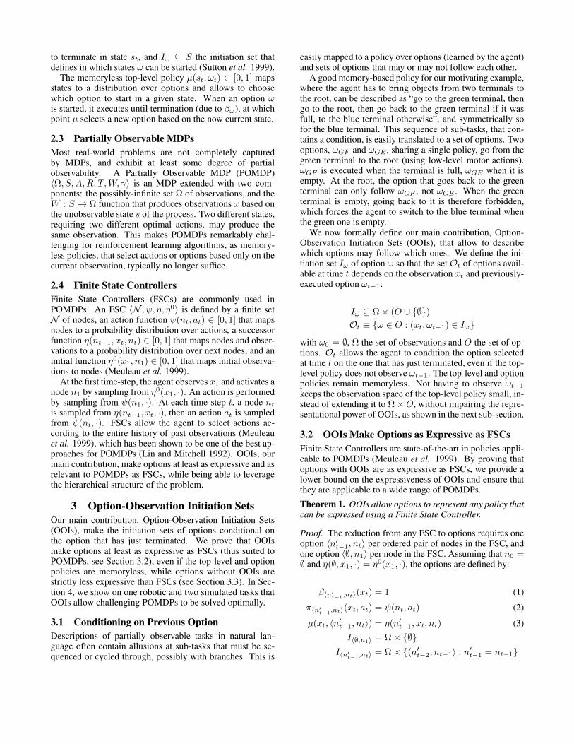
Figure 3: Two-nodes Finite State Controller that emits aninfinite sequence ABAB... based on an uninformative ob-servation x∅. This FSC cannot be expressed using optionswithout OOIs.

Each option corresponds to an edge of the FSC. Equa-tion 1 ensures that every option stops after having emitteda single action, as the FSC takes one transition every time-step. Equation 2 maps the current option to the action emit-ted by the destination node of its corresponding FSC edge.We show that µ and I〈n′t−1,nt〉 implement η(nt−1, xt, nt),with ωt−1 = 〈n′t−2, nt−1〉, by:

µ(xt, 〈n′t−1, nt〉) =η(nt−1, xt, nt)

〈n′t−2, nt−1〉 ∈ I〈n′t−1,nt〉

⇔ n′t−1 = nt−1

0〈n′t−2, nt−1〉 /∈ I〈n′t−1,nt〉

⇔ n′t−1 6= nt−1

Because η maps nodes to nodes and µ selects optionsrepresenting pairs of nodes, µ is extremely sparse and re-turns a value different from zero, η(nt−1, xt, nt), only when〈n′t−2, nt−1〉 and 〈n′t−1, nt〉 agree on nt−1.

Our reduction uses options with trivial policies, that ex-ecute for a single time-step, which leads to a large amountof options to compensate. In practice, we expect to be ableto express policies for real-world POMDPs with much lessoptions than the number of states an FSC would require, asshown in our simulated (Section 4.4, 2 options) and roboticexperiments (Section 4.3, 12 options). In addition to beingsufficient, the next sub-section proves that OOIs are neces-sary for options to be as expressive as FSCs.

3.3 Original Options are not as Expressive asFSCs

While options with regular initiation sets are able to expresssome memory-based policies (Sutton et al. 1999, page 7),the tiny but valid Finite State Controller presented in Figure3 cannot be mapped to a set of options and a policy overoptions (without OOIs). This proves that options withoutOOIs are strictly less expressive than FSCs.

Theorem 2. Options without OOIs are not as expressive asFinite State Controllers.

Proof. Figure 3 shows a Finite State Controller that emitsa sequence of alternating A’s and B’s, based on a constantuninformative observation x∅. This task requires memorybecause the observation does not provide any informationabout what was the last letter to be emitted, or which onemust now be emitted. Options having memoryless policies,

options executing for multiple time-steps are unable to rep-resent the FSC exactly. A combination of options that exe-cute for a single time-step cannot represent the FSC either,as the options framework is unable to represent memory-based policies with single-time-step options (Sutton et al.1999).

4 ExperimentsThe experiments in this section illustrate how OOIs allowagents to perform optimally in environments where optionswithout OOIs fail. Section 4.3 shows that OOIs allow theagent to learn an expert-level policy for our motivating ex-ample (Section 1.1). Section 4.4 shows that the top-level andoption policies required by a repetitive task can be learned,and that learning option policies allow the agent to lever-age random OOIs, thereby removing the need for designingthem. In Section 4.5, we progressively reduce the amountof options available to the agent, and demonstrate how OOIsstill allow good memory-based policies to emerge when asub-optimal amount of options are used.

All our results are averaged over 20 runs, with standarddeviation represented by the light regions in the figures. Thesource code, raw experimental data, run scripts, and plottingscripts of our experiments, along with a detailed descriptionof our robotic setup, are available as supplementary mate-rial. A video detailing our robotic experiment is available athttp://steckdenis.be/oois_demo.mp4.

4.1 Learning AlgorithmAll our agents learn their top-level and option policies (if notprovided) using a single feed-forward neural network, withone hidden layer of 100 neurons, trained using Policy Gra-dient (Sutton et al. 2000) and the Adam optimizer (Kingmaand Ba 2014). Our neural network π takes three inputs andproduces one output. The inputs are problem-specific ob-servation features x, the one-hot encoded current option ω(ω = 0 when executing the top-level policy), and a mask,mask. The output y is the joint probability distribution overselecting actions or options (so that the same network can beused for the top-level and option policies), while terminatingor continuing the current option:

h1 = tanh(W1[xTωT ]T + b1),

y = σ(W2h1 + b2) mask,

y =y

1T y,

with Wi and bi the trainable weights and biases of layer i, σthe sigmoid function, and the element-wise product of twovectors. The fraction ensures that a valid probability dis-tribution is produced by the network. The initiation sets ofoptions are implemented using the mask input of the neu-ral network, a vector of 2 × (|A| + |O|) integers, the samedimension as the y output. When executing the top-levelpolicy (ω = 0), the mask forces the probability of primitiveactions to zero, preserves option ωi according to Iωi

, and

prevents the top-level policy from terminating. When exe-cuting an option policy (ω 6= 0), the mask only allows prim-itive actions to be executed. For instance, if there are twooptions and three actions, mask = end

cont (0 0 1 1 10 0 1 1 1 ) when

executing any of the options. When executing the top-levelpolicy, mask = end

cont (0 0 0 0 0a b 0 0 0 ), with a = 1 if and only if

the option that has just finished is in the initiation set of thefirst option, and b = 1 according to the same rule but for thesecond option. The neural network π is trained using PolicyGradient, with the following loss:

L(π) = −T∑t=0

(Rt − V (xt, ωt)) log(π(xt, ωt, at))

with at ∼ π(xt, ωt, ·) the action executed at time t. The re-turnRt =

∑Tτ=t γ

τrτ , with rτ = R(sτ , aτ , sτ+1), is a sim-ple discounted sum of future rewards, and ignores changesof current option. This gives the agent information about thecomplete outcome of an action or option, by directly eval-uating its flattened policy. A baseline V (xt, ωt) is used toreduce the variance of the L estimate (Sutton et al. 2000).V (xt, ωt) predicts the expected cumulative reward obtain-able from xt in option ωt using a separate neural network,trained on the monte-carlo return obtained from xt in ωt.

4.2 Comparison with LSTM over OptionsIn order to provide a complete evaluation of OOIs, a variantof the π and V networks of Section 4.1, where the hiddenlayer is replaced with a layer of 20 LSTM units (Hochre-iter and Schmidhuber 1997; Sridharan et al. 2010), is alsoevaluated on every task. We use 20 units as this leads to thebest results in our experiments, which ensures a fair compar-ison of LSTM against OOIs. In all experiments, the LSTMagents are provided the same set of options as the agent withOOIs. Not providing any option, or less options, leads toworse results. Options allow the LSTM network to focus onimportant observations, and reduces the time horizon to beconsidered. Shorter time horizons have been shown to bebeneficial to LSTM (Bakker 2001).

Despite our efforts, LSTM over options only manages tolearn good policies in our robotic experiment (see Section4.3), and requires more than twice the amount of episodesas OOIs to do so. In our repetitive task, dozens of repe-titions seem to confuse the network, that quickly divergesfrom any good policy it may learn (see Section 4.4). OnTreeMaze, a much more complex version of the T-mazetask, originally used to benchmark reinforcement learningLSTM agents (Bakker 2001), the LSTM agent learns the op-timal policy after more than 100K episodes (not shown onthe figures). These results illustrate how learning with recur-rent neural networks is sometimes difficult, and how OOIsallow to reliably obtain good results, with minimal engineer-ing effort.

4.3 Object GatheringThe first experiment illustrates how OOIs allow an expert-level policy to be learned for a complex robotic partially-observable repetitive task. The experiment takes place in the

4

5

6

7

8

9

10

11

12

0K 5K 10K 15K 20K 25K 30K 35K

Cum

ulat

ive

rew

ard

per e

piso

de

Episode

LSTM + OptionsOOIs + Options

OptionsExpert Policy

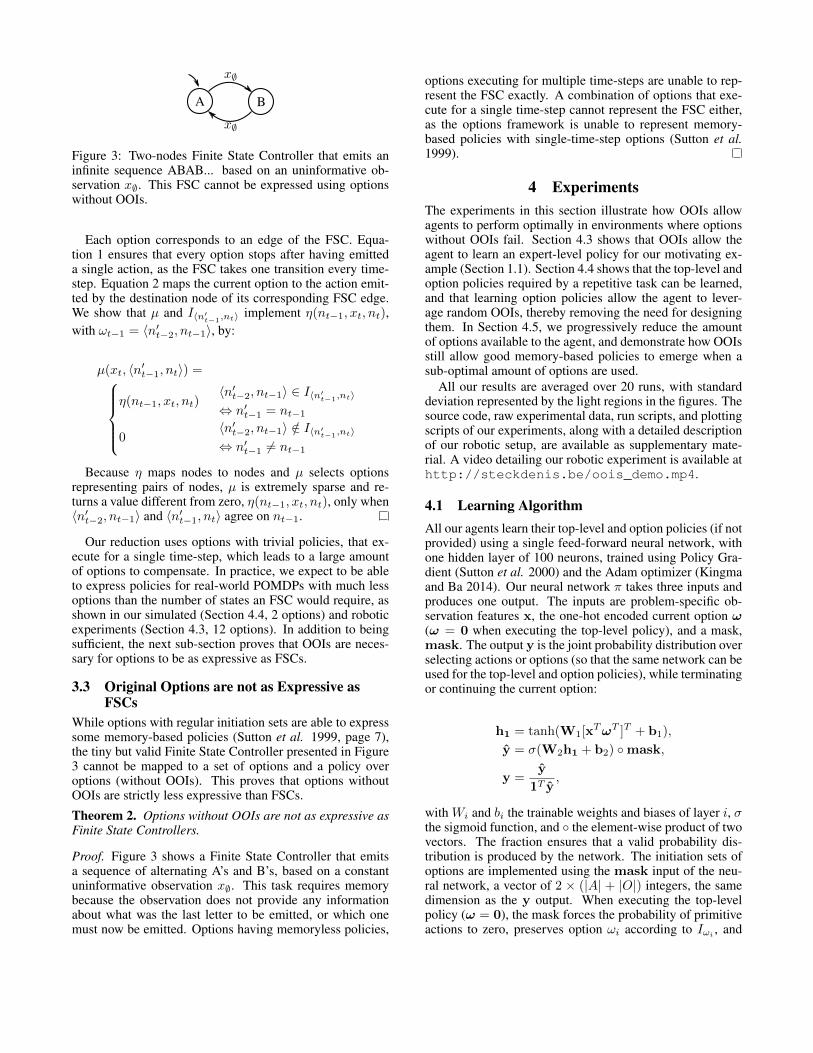
Figure 4: Cumulative reward per episode obtained on ourobject gathering task, with OOIs, without OOIs, and usingan LSTM over options. OOIs learns an expert-level policymuch quicker than an LSTM over options. The LSTM curveflattens-out (with high variance) after about 30K episodes.

environment described in Section 1.1. A robot has to gatherobjects one by one from two terminals, green and blue, andbring them back to the root location. Because our actualrobot has no effector, it navigates between the root and theterminals, but only pretends to move objects. The agent re-ceives a reward of +2 when it reaches a full terminal, -2when the terminal is empty. At the beginning of the episode,each terminal contains 2 to 4 objects, this amount being se-lected randomly for each terminal. When the agent goes toan empty terminal, the other one is re-filled with 2 to 4 ob-jects. The episode ends after 2 or 3 emptyings (combinedacross both terminals). Whether a terminal is full or emptyis observed by the agent only when it is at the terminal. Theagent therefore has to remember information acquired at ter-minals in order to properly choose, at the root, to which ter-minal it will go.

The agent has access to 12 memoryless options that goto red (ωR1..R4), green (ωG1..G4) or blue objects (ωB1..B4),and terminate when the agent is close enough to them toread a QR-code displayed on them. The initiation set ofωR1,R2 is ωG1..G4, of ωR3,R4 is ωB1..B4, and of ωGi,Bi isωRi∀i = 1..4. This description of the options and their

OOIs is purposefully uninformative, and illustrates how lit-tle information the agent has about the task. The option setused in this experiment is also richer than the simple exam-ple of Section 3.1, so that the solution of the problem, notgoing back to an empty terminal, is not encoded in OOIs butmust be learned by the agent.

Agents with and without OOIs learn top-level policiesover these options. We compare them to a fixed agent,using an expert top-level policy that interprets the op-tions as follows: ωR1..R4 go to the root from a full/emptygreen/blue terminal (and are selected accordingly at the ter-minals depending on the QR-code displayed on them), whileωG1..G4,B1..B4 go to the green/blue terminal from the rootwhen the previous terminal was full/empty and green/blue.At the root, OOIs ensure that only one option amongst go togreen after a full green, go to green after an empty blue, goto blue after a full blue and go to blue after an empty greenis selected by the top-level policy: the one that corresponds

to what color the last terminal was and whether it was fullor empty. The agent goes to a terminal until it is empty, thenswitches to the other terminal, leading to an average rewardof 10.2

When the top-level policy is learned, OOIs allow the taskto be solved, as shown in Figure 4, while standard initiationsets do not allow the task to be learned. Because experimentson a robot are slow, we developed a small simulator for thistask, and used it to produce Figure 4 after having success-fully asserted its accuracy using two 1000-episodes runs onthe actual robot. The agent learns to properly select optionsat the terminals, depending on the QR-code, and to output aproper distribution over options at the root, thereby match-ing our expert policy. The LSTM agent learns the policy too,but requires more than twice the amount of episodes to doso. The high variance displayed in Figure 4 comes from thevarying amounts of objects in the terminals, and the randomselection of how many times they have to be emptied.

Because fixed option policies are not always available, wenow show that OOIs allow them to be learned at the sametime as the top-level policy.

4.4 Modified DuplicatedInputIn some cases, a hierarchical reinforcement learning agentmay not have been provided policies for several or any of itsoptions. In this case, OOIs allow the agent to learn its top-level policy, the option policies and their termination func-tions. In this experiment, the agent has to learn its top-leveland option policies to copy characters from an input tape toan output tape, removing duplicate B’s and D’s (mappingABBCCEDD to ABCCED for instance; B’s and D’s alwaysappear in pairs). The agent only observes a single input char-acter at a time, and can write at most one character to theoutput tape per time-step.

The input tape is a sequence of N symbols x ∈ Ω, withΩ = A,B,C,D,E and N a random number between20 and 30. The agent observes a single symbol xt ∈ Ω,read from the i-th position in the input sequence, and doesnot observe i. When t = 1, i = 0. There are 20 actions(5×2×2), each of them representing a symbol (5), whetherit must be pushed onto the output tape (2), and whether ishould be incremented or decremented (2). A reward of 1is given for each correct symbol written to the output tape.The episode finishes with a reward of -0.5 when an incorrectsymbol is written.

The agent has access to two options, ω1 and ω2. OOIsare designed so that ω2 cannot follow itself, with no such re-striction on ω1. No reward shaping or hint about what eachoption should do is provided. The agent automatically dis-covers that ω1 must copy the current character to the output,and that ω2 must skip the character without copying it. Italso learns the top-level policy, that selects ω2 (skip) whenobserving B or D and ω2 is allowed, ω1 otherwise (copy).

Figure 5 shows that an agent with two options and OOIslearns the optimal policy for this task, while an agent with

2 2+32

× (−2 + 2+42

× 2), 2 or 3 emptyings of terminals thatcontain 2 to 4 objects. Average confirmed experimentally from1000 episodes using the policy, p > 0.30.

0

5

10

15

20

0K 20K 40K 60K 80K 100K 120K 140K

Cum

ulat

ive

rew

ard

per e

piso

de

Episode

OOIs + OptionsRnd. OOIs + 16 Options

LSTM + OptionsOptions

Optimal Policy

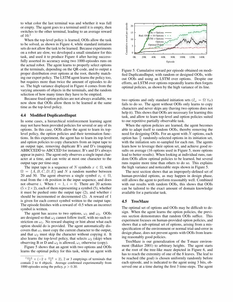
Figure 5: Cumulative reward per episode obtained on modi-fied DuplicatedInput, with random or designed OOIs, with-out OOIs and using an LSTM over options. Despite ourefforts, an LSTM over options repeatedly learns then forgetsoptimal policies, as shown by the high variance of its line.

two options and only standard initiation sets (Iω = Ω ∀ω)fails to do so. The agent without OOIs only learns to copycharacters and never skips any (having two options does nothelp it). This shows that OOIs are necessary for learning thistask, and allow to learn top-level and option policies suitedto our repetitive partially observable task.

When the option policies are learned, the agent becomesable to adapt itself to random OOIs, thereby removing theneed for designing OOIs. For an agent with N options, eachoption has N

2 randomly-selected options in its initiation set,with the initiation sets re-sampled for each run. The agentslearn how to leverage their option set, and achieve good re-sults on average (16 options used in Figure 5, more optionslead to better results). When looking at individual runs, ran-dom OOIs allow optimal policies to be learned, but severalruns require more time than others to do so. This explainsthe high variance and noticeable steps shown in Figure 5.

The next section shows that an improperly-defined set ofhuman-provided options, as may happen in design phase,still allows the agent to perform reasonably well. Combinedwith our results with random OOIs, this shows that OOIscan be tailored to the exact amount of domain knowledgeavailable for a particular task.

4.5 TreeMazeThe optimal set of options and OOIs may be difficult to de-sign. When the agent learns the option policies, the previ-ous section demonstrates that random OOIs suffice. Thisexperiment focuses on human-provided option policies, andshows that a sub-optimal set of options, arising from a mis-specification of the environment or normal trial-and-error indesign phase, does not prevent agents with OOIs from learn-ing reasonably good policies.

TreeMaze is our generalization of the T-maze environ-ment (Bakker 2001) to arbitrary heights. The agent startsat the root of the tree-like maze depicted in Figure 6, andhas to reach the extremity of one of the 8 leaves. The leaf tobe reached (the goal) is chosen uniformly randomly beforeeach episode, and is indicated to the agent using 3 bits, ob-served one at a time during the first 3 time-steps. The agent

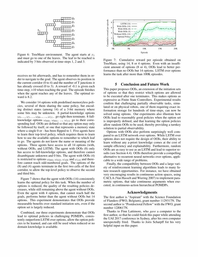
x1

g0

g1g2

g3

g4

g5

g6

g7

Figure 6: TreeMaze environment. The agent starts at x1and must go to one of the leaves. The leaf to be reached isindicated by 3 bits observed at time-steps 1, 2 and 3.

receives no bit afterwards, and has to remember them in or-der to navigate to the goal. The agent observes its position inthe current corridor (0 to 4) and the number of T junctions ithas already crossed (0 to 3). A reward of -0.1 is given eachtime-step, +10 when reaching the goal. The episode finisheswhen the agent reaches any of the leaves. The optimal re-ward is 8.2.

We consider 14 options with predefined memoryless poli-cies, several of them sharing the same policy, but encod-ing distinct states (among 14) of a 3-bit memory wheresome bits may be unknown. 6 partial-knowledge optionsω0−−, ω1−−, ω00−, ..., ω11− go right then terminate. 8 full-knowledge options ω000, ω001, ..., ω111 go to their corre-sponding leaf. OOIs are defined so that any option may onlybe followed by itself, or one that represents a memory statewhere a single 0 or - has been flipped to 1. Five agents haveto learn their top-level policy, which requires them to learnhow to use the available options to remember to which leafto go. The agents do not know the name or meaning of theoptions. Three agents have access to all 14 options (with,without OOIs, and LSTM). The agent with OOIs (8) onlyhas access to full-knowledge options, and therefore cannotdisambiguate unknown and 0 bits. The agent with OOIs (4)is restricted to options ω000, ω010, ω100 and ω110 and there-fore cannot reach odd-numbered goals. The options of the(8) and (4) agents terminate in the first two cells of the firstcorridor, to allow the top-level policy to observe the secondand third bits.

Figure 7 shows that the agent with OOIs (14) consistentlylearns the optimal policy for this task. When the number ofoptions is reduced, the quality of the resulting policies de-creases, while still remaining above the agent without OOIs.Even the agent with 4 options, that cannot reach half thegoals, performs better than the agent without OOIs but 14options. This experiment demonstrates that OOIs providemeasurable benefits over standard initiation sets, even if theoption set is largely reduced.

Combined, our three experiments demonstrate that OOIslead to optimal policies in challenging POMDPs, consis-tently outperform LSTM over options, allow the option poli-cies to be learned, and can still be used when reduced or nodomain knowledge is available.

0

2

4

6

8

0K 5K 10K 15K 20K

Cum

ulat

ive

rew

ard

per e

piso

de

Episode

LSTM (14)With OOIs (14)

With OOIs (8)With OOIs (4)

Without OOIs (14)Optimal Policy

Figure 7: Cumulative reward per episode obtained onTreeMaze, using 14, 8 or 4 options. Even with an insuffi-cient amount of options (8 or 4), OOIs lead to better per-formance than no OOIs but 14 options. LSTM over optionslearns the task after more than 100K episodes.

5 Conclusion and Future WorkThis paper proposes OOIs, an extension of the initiation setsof options so that they restrict which options are allowedto be executed after one terminates. This makes options asexpressive as Finite State Controllers. Experimental resultsconfirm that challenging partially observable tasks, simu-lated or on physical robots, one of them requiring exact in-formation storage for hundreds of time-steps, can now besolved using options. Our experiments also illustrate howOOIs lead to reasonably good policies when the option setis improperly defined, and that learning the option policiesallow random OOIs to be used, thereby providing a turnkeysolution to partial observability.

Options with OOIs also perform surprisingly well com-pared to an LSTM network over options. While LSTM overoptions does not require the design of OOIs, their ability tolearn without any a-priori knowledge comes at the cost ofsample efficiency and explainability. Furthermore, randomOOIs are as easy to use as an LSTM and lead to superior re-sults (see Section 4.4). OOIs therefore provide a compellingalternative to recurrent neural networks over options, appli-cable to a wide range of problems.

Finally, the compatibility between OOIs and a large vari-ety of reinforcement learning algorithms leads to many fu-ture research opportunities. For instance, we have obtainedvery encouraging results in continuous action spaces, usingCACLA (Van Hasselt and Wiering 2007) to implement para-metric options, that take continuous arguments when exe-cuted, in continuous-action hierarchical POMDPs.

AcknowledgmentsThe first author is “Aspirant” with the Science Foundationof Flanders (FWO, Belgium), grant number 1129317N. Thesecond author is “Postdoctoral Fellow” with the FWO, grantnumber 12J0617N.

Thanks to Finn Lattimore, who gave a computer to thefirst author, so that he could finish this paper while attendingthe UAI 2017 conference in Sydney, after his own computerunexpectedly fried. Thanks to Joris Scharpff for his veryhelpful input on this paper.

References[Angeline et al. 1994] Peter J. Angeline, Gregory M. Saunders, and

Jordan B. Pollack. An evolutionary algorithm that constructs re-current neural networks. IEEE Transactions on Neural Networks,5(1):54–65, 1994.

[Bakker 2001] Bram Bakker. Reinforcement learning with longshort-term memory. In Advances in Neural Information ProcessingSystems (NIPS), volume 14, 2001.

[Barto and Mahadevan 2003] Andrew G Barto and Sridhar Ma-hadevan. Recent advances in hierarchical reinforcement learn-ing. Discrete Event Dynamic Systems: Theory and Applications,13(12):341–379, 2003.

[Boots et al. 2011] Byron Boots, Sajid M. Siddiqi, and Geoffrey J.Gordon. Closing the learning-planning loop with predictive staterepresentations. The International Journal of Robotics Research,30(7):954–966, 2011.

[Cassandra et al. 1994] A Cassandra, L Kaelbling, and M Littman.Acting optimaly in partially observable stochastic domains. In Pro-ceedings of the 12th AAAI National Conference on Artificial Intel-ligence, volume 2, pages 1023–1028, 1994.

[Graves et al. 2016] Alex Graves, Greg Wayne, Malcolm Reynolds,Tim Harley, Ivo Danihelka, Agnieszka Grabska-Barwinska, Ser-gio Gomez Colmenarejo, Edward Grefenstette, Tiago Ramalho,John Agapiou, Adria Puigdomenech Badia, Karl Moritz Hermann,Yori Zwols, Georg Ostrovski, Adam Cain, Helen King, Christo-pher Summerfield, Phil Blunsom, Koray Kavukcuoglu, and DemisHassabis. Hybrid computing using a neural network with dynamicexternal memory. Nature, 538(7626):471–476, 2016.

[He et al. 2011] Ruijie He, Emma Brunskill, and Nicholas Roy. Ef-ficient planning under uncertainty with macro-actions. Journal ofArtificial Intelligence Research (JAIR), 40:523–570, 2011.

[Hochreiter and Schmidhuber 1997] Sepp Hochreiter and Jur-gen Jurgen Schmidhuber. Long short-term memory. NeuralComputation, 9(8):1–32, 1997.

[Jozefowicz et al. 2015] Rafal Jozefowicz, Wojciech Zaremba, andIlya Sutskever. An empirical exploration of recurrent network ar-chitectures. In Proceedings of the 32nd International Conferenceon Machine Learning (ICML), pages 2342–2350, 2015.

[Kaelbling et al. 1998] Leslie Pack Kaelbling, Michael L Littman,and Anthony R Cassandra ’. Planning and acting in partially ob-servable stochastic domains. Artificial Intelligence, 101:99–134,1998.

[Kingma and Ba 2014] Diederik Kingma and Jimmy Ba. Adam: Amethod for stochastic optimization. CoRR, abs/1412.6980, 2014.

[Lin and Mitchell 1992] Long-Ji Lin and Tom M Mitchell. Mem-ory approaches to reinforcement learning in non-Markovian do-mains. Carnegie-Mellon University. Department of Computer Sci-ence, 1992.

[Lin and Mitchell 1993] Long-Ji Lin and Tom M Mitchell. Rein-forcement learning with hidden states. From Animals to Animats,2:271–280, 1993.

[Littman et al. 2001] Michael L: Littman, Richard S. Sutton, andSatinder Singh. Predictive Representations of State. In Advances inNeural Information Processing Systems (NIPS), volume 14, pages1555–1561, 2001.

[Meuleau et al. 1999] Nicolas Meuleau, Leonid Peshkin, Kee-eungKim, and Leslie Pack Kaelbling. Learning Finite-State Controllersfor partially observable environments. In Proceedings of the 15thConference on Uncertainty in Artificial Intelligence (UAI), pages427–436, 1999.

[Mikolov et al. 2014] Tomas Mikolov, Armand Joulin, SumitChopra, Michael Mathieu, and Marc’Aurelio Ranzato. Learn-ing longer memory in recurrent neural networks. CoRR,abs/1412.7753, 2014.

[Mnih et al. 2016] Volodymyr Mnih, Adria Puigdomenech Badia,Mehdi Mirza, Alex Graves, Timothy P Lillicrap, Tim Harley, DavidSilver, and Koray Kavukcuoglu. Asynchronous Methods for DeepReinforcement Learning. In Proceedings of the 33rd InternationalConference on Machine Learning (ICML), volume 48, pages 1928–1937, 2016.

[Peshkin et al. 1999] Leonid Peshkin, Nicolas Meuleau, and LeslieKaelbling. Learning policies with external memory. In Proceed-ings of the 16th International Conference on Machine Learning(ICML), pages 307–314, 1999.

[Precup 2000] Doina Precup. Temporal Abstraction in Reinforce-ment Learning. PhD thesis, University of Massachusetts, 2000.

[Roy et al. 2006] Nicholas Roy, Geoffrey Gordon, and SebastianThrun. Planning under uncertainty for reliable health care robotics.Springer Tracts in Advanced Robotics, 24:417–426, 2006.

[Sridharan et al. 2010] Mohan Sridharan, Jeremy Wyatt, andRichard Dearden. Planning to see: A hierarchical approach toplanning visual actions on a robot using POMDPs. Artificial In-telligence, 174:704–725, 2010.

[Sutton et al. 1999] Richard Sutton, Doina Precup, and SatinderSingh. Between MDPs and semi-MDPs: A framework for tem-poral abstraction in reinforcement learning. Artificial intelligence,112:181–211, 1999.

[Sutton et al. 2000] Richard Sutton, David McAllester, SatinderSingh, and Yishay Mansour. Policy gradient methods for reinforce-ment learning with function approximation. In Advances in NeuralInformation Processing Systems (NIPS), volume 13, 2000.

[Tessler et al. 2016] Chen Tessler, Shahar Givony, Tom Zahavy,Daniel J Mankowitz, and Shie Mannor. A Deep Hierarchical Ap-proach to Lifelong Learning in Minecraft. In 13th European Work-shop on Reinforcement Learning (EWRL), 2016.

[Theocharous 2002] Georgios Theocharous. Hierarchical learningand planning in partially observable Markov decision processes.PhD thesis, Michigan State University, 2002.

[Van Hasselt and Wiering 2007] Hado Van Hasselt and Marco A.Wiering. Reinforcement learning in continuous action spaces. Pro-ceedings of the 2007 IEEE Symposium on Approximate DynamicProgramming and Reinforcement Learning, pages 272–279, 2007.

[Wiering and Schmidhuber 1997] Marco Wiering and JurgenSchmidhuber. HQ-Learning. Adaptive Behavior, 6(2):219–246,1997.

[Zaremba and Sutskever 2015] Wojciech Zaremba and IlyaSutskever. Reinforcement Learning Neural Turing Machines.CoRR, abs/1505.00521, 2015.