Auto -ID CenterMassachusetts Institute of Technology

77 Massachusetts Avenue Cambridge, MA 02139

http://auto-id.mit.edu/

MIT-AUTOID -TR-003 ePC: 21.0000001.05003.XXXXXXXXXX

Efficient Memoryless Protocol for Tag Identification

Ching Law, Kayi Lee, Kai-Yeung Siu

October 2000

MIT-AUTOID-TR-003

Efficient Memoryless Protocol for Tag Identification

Ching Law, Kayi Lee, and Kai-Yeung Siu{ching,kylee,siu}@list.mit.edu

Abstract

This paper presents an efficient collision resolution protocol and its variations for the tag identificationproblem, where an electromagnetic reader attempts to obtain within its read range the unique ID number ofeach tag. The novelty of our main protocol is that each tag is memoryless, i.e., the current response of each tagonly depends on the current query of the reader but not on the past history of the reader’s queries. Moreover,the only computation required for each tag is to match its ID against the binary string in the query. Theoreticalresults in both time and communication complexities are derived to demonstrate the efficiency of our protocols.

Keywords: Radio Frequency Identification, Anti-Collision Algorithms, Conflict Resolution

1 Introduction

Recent advances in low-cost, network-aware embedded processors enable the efficient control of most devices andmachines over an open communication infrastructure ranging from a small home network to the global Internet.Moreover, the emergence of low-power and low-cost sensing technologies also makes it likely that in the near future,a variety of consumer goods will be tagged with remotely readable identification tags. For example, electromag-netic tags, which are being considered to replace Uniform Product Codes (Bar Codes), can be read automaticallyfrom a distance without line-of-sight. This opens up vast new opportunities for implementing smart automatedsystems exhibiting intelligent, collaborative behavior that can drastically improve human productivity and effi-ciency. Example applications include automatic object tracking, inventory and supply chain management, andWeb appliances [1].

Motivated by the need for implementing a low-cost, robust automatic identification system using electromagneticreaders and tags, we consider in this paper a tag identification problem in which a reader attempts to obtain theinformation (a unique identification number) stored in each individual tag within the read range. Because of thesevere cost constraints in implementing these tags in practical applications1, each tag is desired to be passive (i.e.no battery requirement) and can only have minimal built-in computing circuitry. The reader is responsible totransmit certain signals, which will power each individual tag at a distance to respond with its unique ID to thereader.

The natural question is: what protocol should the reader and the tags use so that the ID of each tag can becommunicated to the reader as fast and reliably as possible? Without any coordination among the reader andthe tags, the responses from the tags to the reader can collide, in which case the IDs of the tags will becomeillegible to the reader. This is a special case of the multiple-access communication problem and the solution to thegeneral problem which does not require prior scheduling or central control is often referred to as the collision (orconflict) resolution protocol. This problem has been studied extensively in the past several decades. However, ourapplications introduce a more challenging aspect to the problem. Because of the severe computational and energy

The conference version of this paper appears in the Proceedings of the 4th International Workshop on Discrete Algorithms andMethods for Mobile Computing and Communications, August 11, 2000, Boston, Massachusetts. (In conjunction with ACM Mobicom2000)

This work was supported in part by the MIT Auto-ID Center, with industrial sponsors consisting of the Uniform Code Council,Procter & Gamble, Gillette, International Paper, EAN International and CHEP. Please forward any future correspondence to Kai-YeungSiu at siu@list.mit.edu.

1For example, to replace the Bar Codes with electromagnetic tags, the objective is to bring the manufacturing cost of each tag toless than 1 cent.

1

constraints in each tag, it is unreasonable to assume that the tags can communicate with each other directly andthat they can maintain dynamic states of the communication process in their circuitry.

We present here a novel collision resolution protocol which allows the reader to obtain the ID from each tagwithin its read range, while the computational and memory requirement for each tag is minimal. In fact, the keyfeature of our main protocol is that each tag is memoryless, i.e., the current response of each tag only depends onthe current query of the reader but not on the past history of the reader’s queries. Moreover, the only computationrequired for each tag is to match its ID against the binary string in the query. The rest of the paper is organizedas follows: Section 2 introduces an abstract model for the tag identification problem. Section 3 presents the basicQuery-Tree (QT) protocol. Section 4 discusses related work. Section 5 analyzes the time complexity of the QTprotocol. Section 6 presents a generalization of the QT protocol to handle an unreliable tag-reader communicationchannel. Section 7 analyzes the communication complexity of the QT protocol and introduces two variants forreducing the communication complexity. Concluding remarks are given in Section 8.

2 Tag Identification

A tag identification system consists of one reader and n tags. The reader is a powerful entity with abundantmemory and computation power. On the other hand, the tags are limited in memory and computation power.

There is a single communication channel between the reader and the tags. However, the tags are not able toexchange messages among each other. The reader can broadcast messages to the tags. Upon receiving a message,each tag can optionally send a response back to the reader. If only one tag responds, the reader receives themessage. But if more than one tag respond, their messages would collide on the communication channel, and thuscannot be received by the reader. In this case, the reader detects a collision on the channel but nothing else.

Each tag i ∈ {1, . . . , n} has a unique ID string in {0, 1}k, where k is the length of the ID string. At thebeginning, the reader does not know anything about the tags. A tag identification protocol specifies the algorithmsfor the reader and the tags, so that the reader can collect all the tag IDs.

3 The Query-Tree Protocol

In this section, we will introduce the Query Tree (QT) protocol. Our time and communication complexity analyseswill be based on this protocol. In Section 5.4 we will introduce different variations of the protocol to optimizethe running time. In Section 7 we will introduce the QT-sl and QT-im variants for optimizing the communicationcomplexity.

The QT algorithm consists of rounds of queries and responses. In each round, the reader asks the tags whetherany of their IDs contains a certain prefix. If more than one tag answer, then the reader knows that there are atleast two tags having that prefix. The reader then appends symbol 0 or 1 to the prefix, and continues to queryfor longer prefixes. When a prefix matches a tag uniquely, that tag can be identified. Therefore, by extendingthe prefixes until only one tag’s ID matches, the algorithm can discover all the tags. The following describes theprotocol:The QT Protocol

Let A = ∪ki=0 {0, 1}i be the set of binary strings with length at most k. The state of the reader is a

pair (Q,M), where

1. queue Q is a sequence of strings in A;

2. memory M is a set of strings in A.

A query from the reader is a string q in A.

A reply from a tag is a string w in {0, 1}k.

Reader For convenience, let us define the queue Q be 〈ε〉, where ε is the empty string, and memoryM be empty initially.

1. Let Q = 〈q1, q2, . . . , ql〉.2. Broadcast query q1 to the tags.

3. Update Q to be 〈q2, . . . , ql〉.

2

9

8

7

6

5

4

3

2

001 001

000000

11011

10110

no response01

collision00

collision1

collision

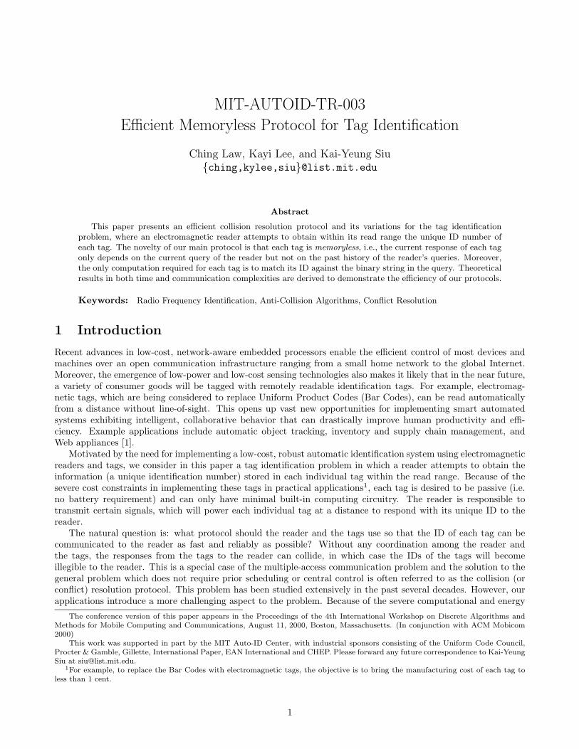
ID: {000, 001, 101, 110}

Query Response�

0

collision

Step

1

Figure 1: Communication between the reader and the tags with the QT Protocol.

4. On receiving the responses from the tags:

• If the reply is string w, then insert string w into memory M .• If a collision is detected at communication channel, then set Q to be〈q2, . . . , ql, q10, q11〉.• If there is no reply, do nothing.

Repeat the above procedure until Q is empty.

Tag Let w = w1w2 · · ·wk be the tag’s ID. Let w be the query string received from the reader. If q = εor q = w1w2 · · ·w|q|, then the tag sends string w to the reader.

We note that when more than one tag try to respond at the same time, the reader will detect a collision insteadof receiving the messages. An example of the communication between the reader and the tags in the protocol isillustrated in Figure 1.

In reality, it is not possible for the reader to send the empty string ε. Thus, in practice, the protocol shouldstart with strings 0 and 1. This will only improve the performance unless there is only one tag, since otherwise theempty string will guarantee a conflict.

4 Related Work

Before presenting the analysis of the QT protocol, we first discuss related previous work.Our QT protocol is closely related to conflict resolution algorithms in the area of multiple access communication

[6, 11, 2]. Since our QT protocol is designed for tag identification, which is quite different from those applicationsconsidered in prior research on conflict resolution protocols, the specific mechanism of our protocol is also quitedifferent. However, the underlying algorithm shares similar insights with previous work. Conflict resolution algo-rithms were introduced by Capetanakis [3], and Tsybakov and Mikhailov [11]. It was further studied by Massey[7], Fayolle et al. [5], and Mathys and Flajolet [8]. In particular, [8] contains a detailed theoretical treatment. Fora comprehensive survey and a bibliography on conflict resolution algorithms, see Molle and Polyzos [9].

Since conflict resolution algorithms have already been widely studied, our discussion will focus on the propertiesof the QT protocol as applied to the problem of tag identification. In particular, we note the following differencesbetween the tag identification problem and the general multiple access communication problem:

• The tags are very limited in computational power and memory, whereas computation and memory are notthe limiting constraints in multiple access communication.

• The number of tags in our problem is fixed during the run of the algorithm, whereas the general multipleaccess problem usually models network traffic as a stochastic process.

• Communication bandwidth is much more constrained in the tag identification problem than in the generalmultiple access problem. Thus it is highly desirable to reduce the number of bits transmitted in the tagidentification problem. This will be further discussed in Section 7.

3

• When fault tolerance issues are considered, the fault model in the tag identification problem is also differentfrom the general multiple access problem. We will discuss the issue of fault tolerance in Section 6.

We also want to emphasize the following characteristics of the QT protocol:

• The tags are memoryless: a tag’s response depends on the current query and its tag ID only.

• The QT protocol is deterministic and does not assume any randomization technique.

• The only computation required for a tag is prefix-matching its own predetermined ID.

Chan et al. [4] suggests a direct implementation of a conflict resolution algorithm commonly studied in pre-vious work for the tag identification problem. However, we note that this approach suffers from the followingshortcomings.

• A log2 k-bit register is needed to store certain state information in each tag.

• Each tag needs to be able to increment and decrement its counter.

• Each tag needs to generate a random bit at each step.

• The number of bits sent by each tag is large compared to our QT-sl protocol to be introduced in Section 7.In fact, the algorithm in [4] is optimized for the number of messages sent by the reader, while our Query-Treealgorithm is optimized for implementation simplicity and power consumption.

5 Time Complexity

In this section, we analyze the time complexity of the QT protocol. Assuming that each query-response step takesa fixed amount of time, we count the number of queries sent by the reader in a complete execution of the protocol.We define the identification time of the QT protocol, denoted by TS , as the number of queries sent by the readerin order to identify a set S of tags. As we have discussed in the preceding section, the underlying algorithm of QTis similar to the conflict resolution algorithms studied in some previous work. Using similar analysis from [7], wecan show that for n = |S| ≥ 4,

2.881n− 1 ≤ E [TS ] ≤ 2.887n− 1 (1)

for a uniformly distributed random set S, where E [TS ] is the expected identification time. This gives us the averagetime complexity of the QT protocol. In Section 5.2, we discuss the worst-case time complexity of the protocol. Weshow that in the worst case, it takes n · (k+ 2− log n) steps to identify all the n tags. In Section 5.3, we argue thatwith high probability, the running time of the protocol is O(n).

To help our analysis in the current section and subsequent sections, we introduce the notion of a query tree,which describes the complete dialogue between the reader and the tags in an execution of the QT protocol. Knowingthe size of the query tree, we can find out the identification time of the QT protocol.

5.1 Query Tree

A query tree is a full binary tree (a binary tree in which each node has either two children or no children) capturingthe complete reader-tags dialogue of the QT protocol. For a given execution of the protocol, there is a one-to-onecorrespondence between every node in the query tree and every query sent by the reader. Therefore, the size, i.e.number of nodes, in the query tree is equal to the number of queries sent by the reader.

For any node x in the query tree, let l(x) and r(x) be the left child and right child of x respectively. If x is aleaf node, then l(x) and r(x) are defined to be NIL.

Definition of a Query Tree

Suppose in an execution of the QT protocol, the reader has sent the set Q of query strings. The query tree of theQT protocol execution is defined recursively by Q.

1. The root of the query tree corresponds to the query string ε.

4

b1�

000 001

101 110

internal node

black leaf�

white leaf�

Figure 2: The query tree for the example in Figure 1

2. If the query tree node x corresponds to the query string q, and both q0, q1 ∈ Q, then l(x) and r(x) are querytree nodes that correspond to the query strings q0 and q1 respectively. Otherwise, both l(x) and r(x) equalNIL.

The above definition implies that an internal node of a query tree corresponds to a query string that resultsin a collision in the communication channel. On the other hand, a leaf corresponds to a query string that resultsin either no reply or a response from exactly one tag. To facilitate our discussion, we shall call a leaf white if thecorresponding query string results in no reply, and black otherwise. Figure 2 shows the query tree for the examplein Figure 1.

Structure of a Query Tree

From the definition of query tree, we have the following observations:

1. The height of a query tree is at most k, since the query string sent out by the reader is at most k bits long.

2. If x is an internal node, then x has at least two black leaf descendants. This follows from the fact that eachblack leaf corresponds to a unique tag ID and each internal node corresponds to a query that results in acollision.

5.2 Worst-Case Time Complexity

The number of queries sent by the reader equals the size of the query tree. Given a set S of n tags, let YS be thequery tree for S. Also, let RS be number of internal nodes in the tree YS . Since a query tree is a full binary tree,the size of the tree is simply 2RS + 1.

A simple argument can give a bound on the size of YS . In a query tree, any internal node is an ancestor ofsome black leaf. For each black leaf, it has at most k ancestors, which are internal nodes. This gives us RS ≤ kn.Therefore, it follows that the size of the tree equals 2RS + 1, which is no more than 2nk + 1.

An improved result is stated in the following:

Theorem 1 The number of queries sent by the reader to identify n tags is at most n · (k + 2− log n).

Proof. The number of queries sent by the reader to identify n tags equals the size of the corresponding query tree,which has exactly n black leaves. In Appendix A, it is shown that the size of any query tree with exactly n blackleaves is no more than n · (k + 2− log n).

5

5.3 Probabilistic Analysis

Here we show that with high probability, the running time of the QT protocol is O(n).Mathys and Flajolet [8] claimed that the variance of the running time can be shown to be linear in n, as n→∞.

This would be sufficient to show that the running time is linear in n with high probability. However, the derivationwas omitted in [8] because it is “rather lengthy and complicated”.

In the following we will present a proof that QT has linear running time with high probability. We note that bybounding the number of white leaves (as introduced in Section 5), we essentially bound the total size of the tree.

Let Wn be the random variable of the number of white leaves in a query tree with n black leaves. We will applythe Chernoff bound on the upper tail of the distribution of Wn.

We first need the following technical lemma.

Lemma 1 For n ≥ 2,

E[e0.4Wn

]≤ e0.4n.

Proof. See Appendix B.

Lemma 2

Pr {Wn ≥ a} ≤ e0.4(n−a).

Proof. See Appendix B.

We now show that the running time of QT is O(n) with high probability. In particular, the probability thatQT takes at least cn steps decreases exponentially with size n.

Theorem 2 The probability the QT protocol takes at least cn steps to identify n tags is at most e−0.4n(c/2−2).

Proof. When the size of the query tree is larger than cn − 1, the number of white leaves is at least cn/2 − n. ByLemma 2,

Pr {Wn ≥ a} ≤ e−0.4(a−n)

for all a > 0. Let a = cn/2− n, then,

Pr {Wn ≥ cn/2− n} ≤ e−0.4((cn/2−n)−n)

= e−0.4n(c/2−2).

5.4 Further Enhancement

Here we discuss several techniques of reducing the running time of the QT protocol.

5.4.1 Shortcutting

Consider any internal node of the query tree. This corresponds to a collision for certain prefix q during an executionof the QT protocol. The algorithm will continue to search for the tags by appending 1 and 0 to the prefix q. Withoutloss of generality, assume that the algorithm chooses to search for 0 first. If it turns out that there are no tags withprefix q0, then we know that there are at least two tags with prefix q1. Therefore, the reader should as well skipthe prefix q1.

In the shortcutting QT algorithm, the reader can randomly choose the order of sending q1 and q0. But thiswould be unnecessary if we assume that the tag IDs are uniformly distributed.

This technique is similar to the modified conflict resolution algorithm in the literature [7, 8], and has beenshown to give an improved expected running time bound of 2.665n− 1.

6

5.4.2 Aggressive Advancement

Assume the reader knows that there are at least n unrecognized tags with prefix q. For example, this could be ana prior knowledge: maximum number of items in a checkout counter. Or the reader can detect the strength of theresponse from the tags to estimate the number of tags. When n is large, it is very likely that the responses for q1 andq0 will collide. The probability that either one of the queries does not result in a collision is 2 · ( 1

2n +n · 12n ) = n+1

2n−1 .Now suppose we extend the prefix string by two bits. That is, the reader will query q00, q01, q10, and q11. In thiscase, we save two queries q1 and q0 with probability 1 − n+1

2n−1 . Note that we send more queries (campared withthe original QT protocol) only in the case where both q0 and q1 have exactly one tag with a matching prefix. Thiscannot happen when n ≥ 3.

This technique is equivalent to the “Q-ary tree conflict resolution” as analyzed by [8], which showed that a3-ary tree is optimal without shortcutting, but the basic 2-ary tree is preferred if shortcutting is used.

5.4.3 Categorization

If the reader has some information about the types of the tags, then it is possible to speed up the protocol. Forexample, suppose a set S of IDs is given. Assume the reader knows that set S can be partitioned into S1, . . . , Smsuch that all IDs in Si have prefix qi. Now the reader can just identify each set Si independently. In particular,if we can partition the tags into m groups, then the upper bound on the expected running time is improved to2.887n−m.

6 Fault Tolerance

We now introduce a dynamic version of the QT protocol that is useful when the communication between the tagsand the reader is unreliable. We assume that there is a probability p that a given tag would fail to reply to a query.We assume that these failures are statistically independent events. During any execution of the QT protocols, sometags may not be identified due to these failures. We will develop a QT algorithm with multiple tries such that theprobability of missing any tags is low.

It is impossible to identify all tags with 100% certainty if we want our protocol to terminate. Instead, ouralgorithm is designed to trade off between running time and the probability of missing some tags. In particular,in the QTl protocol, if the reader receives no collision on a query string q, it will repeat sending the the samequery string until it detects a collision or the same query has been sent for l times. The reader will summarizethe responses to all such queries and determine whether there are multiple, one or no tags having the prefix q.Specifically, while the reader is repeatedly sending the query string, it will summarize the responses as follows:

• If the reader detects a collision for the query string, it will conclude that more than one tag have a matchingprefix.

• If in the course of the l queries, no tag has replied, the reader will conclude that no tag has a matching prefix.

• If in the course of the l queries, it receives response(s) from exactly one tag, the reader will conclude thatonly the tag has a matching prefix.

• If in the course of the l queries, it receives responses from different tags, the reader will conclude that morethan one tag have a matching prefix. It will then behave as if a collision is detected.

Since the same query string is sent for multiple times, it is unlikely that a tag with a matching prefix is notidentified.

Theorem 3 With failure probability p ≤ 1/2, the expected running time of the QTl protocol is at most 3l+92 n− 1.

Proof. See Appendix C

Theorem 4 With failure probability p, the probability that the QTl protocol does not recognize a particular tag isat most pl.

Proof. Consider an arbitrary tag w. For the tag w to be unidentified, the reader must have repeated sending someprefix of w for l times. In addition, the tag w must have failed to respond to all these l queries. The probabilityfor this to happen is at most pl.

7

Corollary 1 With failure probability p, the probability that the QT(c+1) log1/p n protocol does not identify all tags isat most 1/nc.

Proof. The probability that a certain tag is not identified is at most p(c+1) log1/p n. Therefore, the probability thatany tag is unidentified is at most np(c+1) log1/p n = 1/nc.

7 Communication Complexity

In this section we turn our attention to the communication complexity of the protocol. The reader communicationcomplexity is the number of bits sent by the reader; and the tag communication complexity is the number of bitssent by a tag. The tag communication complexity is especially important because it is desirable to minimize thepower consumption of the tags.

We will first derive the communication complexities of our QT protocol and then introduce several variants thatimprove upon the performance of QT.

7.1 Basic Query-Tree

In the followings, we will first find the expected number of collisions experienced by a tag. We assume that the bitlength k of each tag ID is infinite. This will give us an upper bound for cases where k is finite. We show that inthe QT protocol, the expected number of responses a tag makes is no more than 2.21 log2 n+ 3.19, where n is thetotal number of tags.

In the algorithm QT, each tag responds to query strings that match its prefix. It will experience a collision onlyif there is some other tag having the same prefix, which is the query string sent by the reader.

Let w be the ID of an arbitrary tag in a set of n tags, in which the IDs are uniformly distributed. Let Cw be thenumber of collisions the tag experiences during the execution of the QT protocol. In addition, let Ijw, j = 0, 1, 2, . . . ,be an indicator variable such that:

Ijw =

0 if none of any other n− 1 tags has the same

j-bit prefix as w,1 otherwise.

Then we have the following equation:

Cw =∞∑j=0

Ijw.

By linearity of expectation,

E [Cw] =∞∑j=0

E[Ijw].

Let wj be the j-bit prefix of w. Then for each j = 0, 1, 2, . . . ,

E[Ijw]

= Pr {some other tag ID has prefix wj}= 1− Pr {all other IDs do not have prefix wj}= 1− (Pr {an ID does not have prefix wj})n−1

= 1− (1− 2−j)n−1.

Therefore, the expected number of conflicting responses the tag experiences is given by:

E [Cw] =∞∑j=0

E[Ijw]

=∞∑j=0

(1− (1− 2−j)n−1

). (2)

A bound on E [Cw] is derived in Theorem 5, which depends on the following two technical lemmas.

8

Lemma 3 For all n ≥ 2,

∞∑j=0

2−j(1− 2−j)n <log2 e+ 2e−

23 + e−

13

n+ 1.

Proof. See Appendix D.

Lemma 4

∞∑j=0

1− (1− 2−j)n−1 ≤n−1∑j=1

C

j,

where C = log2 e+ 2e−23 + e−

13 ≈ 3.19.

Proof. See Appendix D.

Now we are ready to state the theorem and prove it.

Theorem 5 For a system with n tags, a tag is expected to experience no more than 2.21 log2 n + 3.19 conflictsbefore it successfully transmits its ID.

Proof. From Equation (2), the expected number of conflicting responses a tag experiences, E [Cw], is given by:

E [Cw] =∞∑j=0

1− (1− 2−j)n−1.

Therefore, by Lemma 4,

E [Cw] ≤n−1∑j=1

C

j,

where C = log2 e+ 2e−23 + e−

13 ≈ 3.19.

This implies

E [Cw] ≤ (1 + ln(n− 1)) · C< 2.21 log2 n+ 3.19.

Theorem 6 Let there be n tags to be identified. The expected reader communication complexity for QT is at most2.89kn. The expected tag communication complexity is at most 2.21k log2 n+ 4.19k.

Proof. Since the expected running time for the QT protocol is at most 2.887n− 1, and the length of each query isat most k. Therefore the expected total number of bits sent by the reader is at most 2.89kn.

Theorem 5 implies that each tag is expected to respond for 3.19 + 2.21 log2 n+ 1 = 4.19 + 2.21 log2 n times. Oneach step, the tag sends a k-bit ID. Therefore, the expected tag communication complexity is at most

2.21k log2 n+ 4.19k.

9

7.2 Short-Long Queries

Now we introduce the QT-sl (Query-Tree short-long) protocol that reduces the number of bits transmitted. Wenote that in QT, a lot of the k-bit responses from the tags would end up in collisions. To minimize these wastes,we can have two types of queries from the reader. The short queries will only induce 1-bit responses from the tags,while the long queries will induce the full tag IDs. The reader will send a long query only when it knows that onlyone tag matches the prefix.The QT-sl Protocol

Let A = ∪ki=0 {0, 1}i be the set of binary strings with length at most k. The state of the reader is a

pair (Q,M), where

1. queue Q is a sequence of strings in A;

2. memory M is a set of strings in A.

A query from the reader is a pair (c, w), where c ∈ {short, long} and w ∈ A.

A reply from a tag is a string 1 or a string in {0, 1}k.

Reader For convenience, let us define the queue Q be 〈ε〉, where ε is the empty string, and memoryM be empty initially.

1. Let Q = 〈q1, q2, . . . , ql〉.2. Broadcast query (short, q1) to the tags.

3. Update Q to be 〈q2, . . . , ql〉.4. On receiving the responses from the tags:

• If the reply is 1, then(a) broadcast query (long, q1) to the tags;(b) insert the resulting response string w into memory M .• If a collision is detected at the communication channel, then set Q to be 〈q2, . . . , ql, q10, q11〉.• If there is no reply, do nothing.

Repeat the above procedure until Q is empty.

Tags Let w = w1w2 · · ·wk be the tag’s ID. Let (c, q) be the query received from the reader. If q = ε orq = w1w2 · · ·w|q|, then

• if command c is short, send string 1 to the reader;

• if command c is long, send string w to the reader.

Theorem 7 Let there be n tags to be identified. The expected reader communication complexity of QT-sl is at most3.89kn+ 3.89n. The expected tag communication complexity of QT-sl is at most 2.21 log2 n+ k + 4.19.

Proof. Note that with QT-sl protocol, we need one extra bit to specify whether the query is short or long.The expected total number of short and long queries is at most 3.887n − 1. Each query is at most k + 1-bit

long, thus the expected reader communication complexity is at most

(3.887n− 1)(k + 1) < 3.89kn+ 3.89n.

Theorem 5 implies that each tag is expected to respond for 4.19 + 2.21 log2 n times. For each short query, thetag sends a 1 response. For the long query, the tag sends a k-bit ID. Therefore, the expected tag communicationcomplexity is at most

2.21 log2 n+ k + 4.19.

10

Reader Tag TotalQT 2.89kn 2.21k log2 n+ 4.19k 2.21kn log2 n+ 7.08knQT-sl 3.89kn+ 3.89n 2.21 log2 n+ k + 4.19 2.21n log2 n+ (8.08 + 4.89k)nQT-im 4.42n log2 n+ 12.18n 2.21 log2 n+ k + 4.19 6.63n log2 n+ (16.37 + k)n

Table 1: Summary of communication complexities of QT, QT-sl, and QT-im. We note that log2 n ≤ k and k is around 96 inpractice.

7.3 Incremental Matching

Here we introduce another technique to further reduce the expected reader communication complexity when log2 nis small compared to k. However, this optimization requires a tag to remember the bit position of the prefix it hasmatched so far. Therefore, the modified protocol is no longer memoryless.

The algorithm QT-im (Query-Tree incremental-matching) is very similar to QT-sl. Thus we will only describethe difference between these two protocols.

First, the QT-im protocol will follow the query tree in a preorder fashion.In QT-im, each tag has a bit marker b ∈ {1, . . . , k}. A tag is active if it has responded 1 in the previous step.

When the tag is active, upon receiving the a query, the tag matches the query string starting from bit b. If thematching is successful, then bit marker b is incremented by 1. Any active tag that mismatches would go into thetransient state. A transient tag will become inactive in the next query unless that query contains the reactivatecommand.

When a long query is received, all tags would reset the bit marker to 1 and become active again. The activetag, upon receiving a long query, will also respond with its full tag ID.

Whenever a short query does not receive any response the reader will send a reactivate query, which isequivalent to a short query except that all transient tags will become active again. Each short command takes 1bit as before, but the reactivate and long commands would need 2 bits each.

With these extra tag functionalities, the reader can then send the prefixes incrementally. For example, if thereader sent q in the previous step and the reader plans to send q0 or q1, it can simply send 0 or 1 instead. Moreover,it is no longer necessary to supply a prefix with the long query.

The tag communication complexity of QT-im is the same as that of QT-sl. However, the number of bits sent bythe reader is reduced.

Theorem 8 The expected reader communication complexity of QT-im protocol is at most 4.42n log2 n+ 12.18n.

Proof. We can partition the queries in groups such that each group ends with a long query. Since exactly one tag isidentified for each group of queries, there are n groups in total. We can find the number of bits transmitted in eachgroup. Theorem 5 implies that on average there are at most 2.21 log2 n+ 3.19 + 1 = 2.21 log2 n+ 4.19 short queriesin a group that result in either a collision or a single response. Since each short query is 2 bits long. The totalnumber of bits transmitted for short queries that result in a collision or a single response, over all the n groups, is:

4.42n log2 n+ 8.38n.

Each long query is 2 bits long. Therefore, in total the reader sends 2n bits for long queries. For each white leaf,the reader sends a 2-bit short query that corresponds to the white leaf, and another 2 bits for the reactivatecommand. Therefore, 4 bits are sent for each white leaf discovered. Equation (1) implies that on average thereare at most 0.444n white leaves. Therefore, the expected reactivate overhead is at most 1.8n. In summary, theexpected reader communication complexity is at most

4.42n log2 n+ 8.38n+ 2n+ 1.8n= 4.42n log2 n+ 12.18n.

7.4 Summary and Comments

Table 1 summarizes the communication complexities of QT, QT-sl, and QT-im, together with simple lower bounds.We showed that we can reduce the communication complexities with the more complicated implementations. Lastly

11

we note that it is possible to achieve O(n) reader communication complexity by implementing reader commands todecrease the bit marker of the tags. Such algorithm (like the one suggested in [4]) would resemble the implementationof the conflict resolution algorithms in computer networking more closely. However, we have decided not to discussit in detail here because the implementation would be too complicated for the tags in practice.

8 Concluding Remarks

In this paper we introduce Query-Tree (QT) as the first memoryless protocol for the tag identification problem.The Query-Tree protocol has simple and deterministic implementation for the tags.

We show that QT runs in n(k + 2 − log2 n) steps in the worst case, but in O(n) time with high probability.In addition, we show that QT can be extended to find all tags with high probability, even if each tag can failindependently during each step. We also study the communication complexity of the QT protocol, and suggest twovariations for further reducing the complexity. The communication complexity results are summarized in Table 1.

We note that given multiple electromagnetic communication channels, the QT protocol can be parallelized. Weare currently investigating how the performance of a parallel QT scales with the number of channels. The basicapproach is to statically assign the channels to different tag ID prefixes, so that the reader will identify the tagsusing the preassigned channel. This approach essentially partitions the set of tags according to their prefixes, sothat each group of tags will be identified independently in parallel.

A more sophisticated approach is to dynamically assign the channels. In this approach, whenever a channel isidle, it will be reused by the reader to communicate with the currently unidentified tags. Therefore, the channelscan be utilized more efficiently.

References

[1] MIT Auto-ID Center. http://auto-id.mit.edu/.

[2] Dimitri Bertsekas and Robert Gallager. Data Networks. Prentice-Hall, second edition, 1992.

[3] J. I. Capetanakis. The Multiple Access Broadcast Channel: Protocol and Capacity Considerations. PhD thesis,1977.

[4] Shun Chan, Harley Heinrich, Dilip Kandlur, and Arvind Krishna. U.S. Patent: Multiple item radio frequencytag identification protocol. Patent number: US5550547. August 1996.

[5] G. Fayolle, P. Flajolet, M. Hofri, and P. Jacquet. Analysis of a stack algorithm for random access communi-cation. IEEE Transactions on Information Theory, IT-31(2):244–254, March 1985. (Special Issue on RandomAccess Communication, J. Massey editor).

[6] Robert G. Gallager. A perspective on multiaccess channels. IEEE Transactions on Information Theory,IT-31(2):124–142, March 1985. (Special Issue on Random Access Communication, J. Massey editor).

[7] J. L. Massey. Collision-resolution algorithms and random-access communications. Multi-User CommunicationSystems, pages 73–99, 1981.

[8] P. Mathys and P. Flajolet. Q-ary collision resolution algorithms in random access systems with free or blockedchannel access. IEEE Transactions on Information Theory, IT-31(2):217–243, March 1985. (Invited Paper,Special Issue on Random Access Communication, J. Massey editor).

[9] Mart L. Molle and George C. Polyzos. Conflict resolution algorithms and their performance analysis. Technicalreport, 1993.

[10] Sheldon Ross. Stochastic Processes. John Wiley & Sons, Inc., second edition, 1996.

[11] Boris Tsybakov. Survey of USSR contributions to random multiple-access communications. IEEE Transactionson Information Theory, IT-31(2):143–165, March 1985. (Special Issue on Random Access Communication, J.Massey editor).

12

p� s

��

r

b2�

s

��

r

b2�

s

��

p�

b1�

q

��

r

b2s

��

r

b2s

(b)

�

p

b1q

(a)

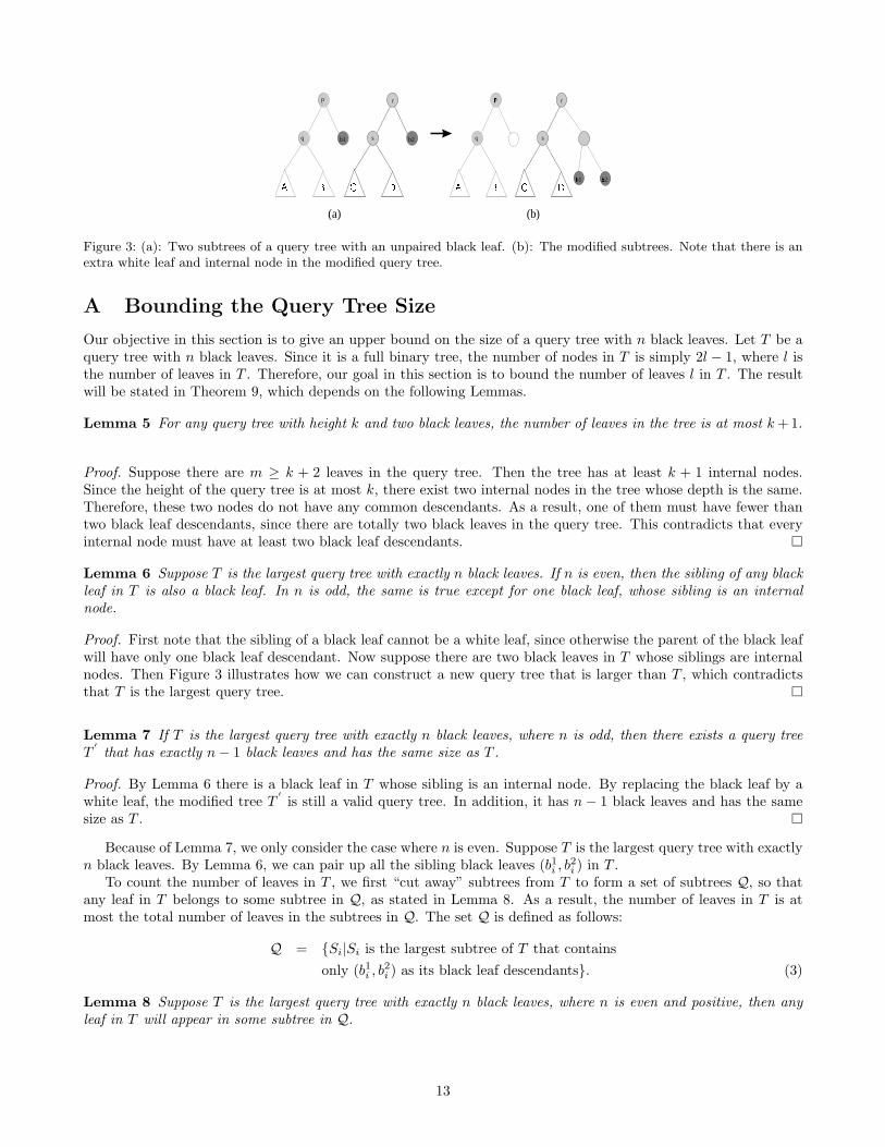
Figure 3: (a): Two subtrees of a query tree with an unpaired black leaf. (b): The modified subtrees. Note that there is anextra white leaf and internal node in the modified query tree.

A Bounding the Query Tree Size

Our objective in this section is to give an upper bound on the size of a query tree with n black leaves. Let T be aquery tree with n black leaves. Since it is a full binary tree, the number of nodes in T is simply 2l − 1, where l isthe number of leaves in T . Therefore, our goal in this section is to bound the number of leaves l in T . The resultwill be stated in Theorem 9, which depends on the following Lemmas.

Lemma 5 For any query tree with height k and two black leaves, the number of leaves in the tree is at most k+ 1.

Proof. Suppose there are m ≥ k + 2 leaves in the query tree. Then the tree has at least k + 1 internal nodes.Since the height of the query tree is at most k, there exist two internal nodes in the tree whose depth is the same.Therefore, these two nodes do not have any common descendants. As a result, one of them must have fewer thantwo black leaf descendants, since there are totally two black leaves in the query tree. This contradicts that everyinternal node must have at least two black leaf descendants.

Lemma 6 Suppose T is the largest query tree with exactly n black leaves. If n is even, then the sibling of any blackleaf in T is also a black leaf. In n is odd, the same is true except for one black leaf, whose sibling is an internalnode.

Proof. First note that the sibling of a black leaf cannot be a white leaf, since otherwise the parent of the black leafwill have only one black leaf descendant. Now suppose there are two black leaves in T whose siblings are internalnodes. Then Figure 3 illustrates how we can construct a new query tree that is larger than T , which contradictsthat T is the largest query tree.

Lemma 7 If T is the largest query tree with exactly n black leaves, where n is odd, then there exists a query treeT′

that has exactly n− 1 black leaves and has the same size as T .

Proof. By Lemma 6 there is a black leaf in T whose sibling is an internal node. By replacing the black leaf by awhite leaf, the modified tree T

′is still a valid query tree. In addition, it has n − 1 black leaves and has the same

size as T .

Because of Lemma 7, we only consider the case where n is even. Suppose T is the largest query tree with exactlyn black leaves. By Lemma 6, we can pair up all the sibling black leaves (b1i , b

2i ) in T .

To count the number of leaves in T , we first “cut away” subtrees from T to form a set of subtrees Q, so thatany leaf in T belongs to some subtree in Q, as stated in Lemma 8. As a result, the number of leaves in T is atmost the total number of leaves in the subtrees in Q. The set Q is defined as follows:

Q = {Si|Si is the largest subtree of T that containsonly (b1i , b

2i ) as its black leaf descendants}. (3)

Lemma 8 Suppose T is the largest query tree with exactly n black leaves, where n is even and positive, then anyleaf in T will appear in some subtree in Q.

13

(b)

y

x

y

xw w

(a)

Figure 4: Modifying a query tree with the structure in (a) into a larger query tree in (b). The tree in (b) has one more whiteleaf and internal node than (a).

Proof. By definition of Q, every black leaf must appear in some subtree in Q. Suppose there is a white leaf x thatdoes not appear in any subtree in Q. Let y denote the parent of x and S denote the subtree rooted at y. Then atleast two pairs of black leaves must appear in S. Suppose only one pair of black leaves appear in S. The fact thatS /∈ Q implies there is a different subtree Si ∈ Q of T such that Si contains the same pair of black leaves and it islarger than S. This implies S is a subtree of Si. Since Si ∈ Q, the white leaf x does not appear in Si. As a result,the fact that x appears in S contradicts that S is a subtree of Si.

Given that at least two pairs of black leaves appear in S, Figure 4 shows the structure of the subtree S. The figureillustrates how we can modify S to construct a new query tree S

′that has one more white leaf than S. If we replace S

by S′

in the query tree T , it would give a new query tree that is larger than T . This contradicts that T is the largestquery tree among all the trees with the same number of black leaves.

As a result, we can count of total number of leaves in Q to give an upper bound of the number of leaves in T .Since every subtree in Q has exactly two black leaves, we can apply Lemma 5 to count the number of leaves ineach subtree.

Now let Q be a set of subtrees constructed according to (3). For each subtree Si ∈ Q, let root(Si) denote theroot of the tree and let depth(Si) denote the depth of the node root(Si) in T .

Lemma 9 −∑Si∈Q depth(Si) ≤ −n2 log n

2 .

Proof. The node root(Si) has depth depth(Si) in the original tree T . Since T is a binary tree, and all the trees inQ are disjoint, if we define h(Si) = 2−depth(Si), we have:∑

Si∈Qh(Si) ≤ 1. (4)

By the fact that the geometric mean of a set of non-negative numbers is at most their arithmetic mean, wehave: ∑

Si∈Qh(Si) ≥ |Q| · (

∏Si∈Q

h(Si))1|Q|

= |Q| · (2∑Si∈Q

−depth(Si))1|Q|

=n

2(2∑Si∈Q

−depth(Si))2n .

Therefore, by Equation (4),n

2(2∑Si∈Q

−depth(Si))2n ≤ 1.

Dividing both sides by n2 , taking the logarithm and then multiplying by n

2 on both sides, we have:∑Si∈Q

−depth(Si) ≤n

2log

2n

= −n2

logn

2.

14

Theorem 9 The total number of leaves in a query tree with height k and n black leaves is at most n2 (k+2− log n).

Proof. Suppose T is the largest query tree with n black leaves. We construct the set of subtrees Q as in (3). Thenthe height of each subtree Si in Q is at most k − depth(Si), since the height of the T is at most k. By Lemma 5,the number of leaves in Si is therefore at most k − depth(Si) + 1. Summing over all the subtrees in Q, the totalnumber of leaves, denoted by L(Q), is given by:

L(Q) ≤∑Si∈Q

((k − depth(Si)) + 1)

= |Q|(k + 1)−∑Si∈Q

depth(Si)

=n

2(k + 1)−

∑Si∈Q

depth(Si)

≤ n

2(k + 1)− n

2log

n

2, by Lemma 9,

=n

2(k + 1− log

n

2).

B Proof of Lemmas 1 and 2 in Subsection 5.3

Lemma 1 For n ≥ 2,

E[e0.4Wn

]≤ e0.4n (5)

Proof. Since W0 = 1 and W1 = 0, we have

E[e0.4W0

]= e0.4,

E[e0.4W1

]= 1.

For n ≥ 2, we have the following recurrence:

E[e0.4Wn

]=

n∑i=0

Pi,n−iE[e0.4(Wi+Wn−i)

], (6)

where Wi and Wn−i are the number of white leaves in the two subtrees. Since Wi and Wn−i are independent, wecan write Equation (6) as

E[e0.4Wn

]=

n∑i=0

Pi,n−iE[e0.4Wi

]E[e0.4Wn−i

](7)

First, for the base case n = 2, we have

E[e0.4W2

]=

2∑i=0

Pi,2−iE[e0.4Wi

]E[e0.4W2−i

]= 2P0,2E

[e0.4W0

]E[e0.4W2

]+ P1,1E

[e0.4W1

]E[e0.4W1

]=

12e0.4E

[e0.4W2

]+

12.

Therefore,

E[e0.4W2

]=

12

1− 12e

0.4

≤ 1.97

< e0.4·2.

15

It remains to show that E[e0.4Wn

]≤ e0.4n for n > 2.

Multiplying both sides of Equation (7) by 2n, we have

2nE[e0.4Wn

]=

n∑i=0

(n

i

)E[e0.4Wi

]E[e0.4Wn−i

]=n−2∑i=2

(n

i

)E[e0.4Wi

]E[e0.4Wn−i

]+ 2(n

0

)E[e0.4W0

]E[e0.4Wn

]+ 2(n

1

)E[e0.4W1

]E[e0.4Wn−1

]=n−2∑i=2

(n

i

)E[e0.4Wi

]E[e0.4Wn−i

]+ 2e0.4E

[e0.4Wn

]+ 2nE

[e0.4Wn−1

](8)

Now, after subtracting both sides of Equation (8) by 2e0.4E[e0.4Wn

], we apply our inductive assumption that

E[e0.4Wi

]≤ e0.4i for i = 2, . . . , n− 1,

(2n − 2e0.4)E[e0.4Wn

]=n−2∑i=2

(n

i

)E[e0.4Wi

]E[e0.4Wn−i

]+ 2nE

[e0.4Wn−1

]≤n−2∑i=2

(n

i

)e0.4ie0.4n−i + 2ne0.4(n−1)

=n−2∑i=2

(n

i

)e0.4n + 2ne0.4ne−0.4

= e0.4n(2n − 2− 2n) + 2ne0.4ne−0.4

= e0.4n(2n − 2e0.4) + 2e0.4ne0.4 − 2e0.4n − 2ne0.4n + 2ne0.4ne−0.4

= e0.4n(2n − 2e0.4) + 2e0.4n((e0.4 − 1)− n(1− e−0.4))

For n > 2,

n(1− e−0.4) > e0.4 − 1.

Thus, we conclude that

(2n − 2e0.4)E[e0.4Wn

]< e0.4n(2n − 2e0.4) (9)

And dividing Equation (9) by 2n − 2e0.4 yields

E[e0.4Wn

]< e0.4n

Lemma 2 Let Wn be the random variable of the number of white leaves in a query tree with n black leaves, then

Pr {Wn ≥ a} ≤ e0.4(n−a).

Proof. The Chernoff Bounds[10, p.39] state that for any random variable X and a > 0,

Pr {X ≥ a} ≤ e−taE[etX]

(10)

for all t > 0.Setting t = 0.4 and X = Wn, we can rewrite Equation (10) as

Pr {Wn ≥ a} ≤ e−0.4aE[e0.4Wn

].

And by Lemma 1, we have

Pr {Wn ≥ a} ≤ e−0.4ae0.4n

= e−0.4(a−n).

16

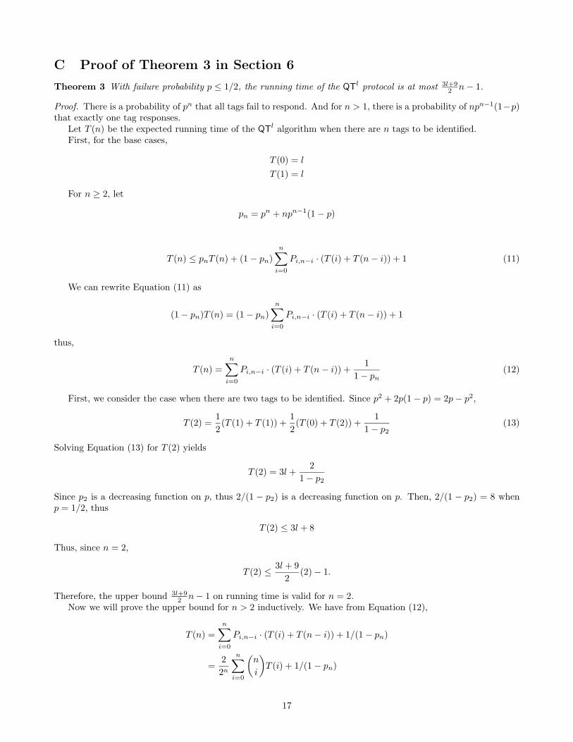
C Proof of Theorem 3 in Section 6

Theorem 3 With failure probability p ≤ 1/2, the running time of the QTl protocol is at most 3l+92 n− 1.

Proof. There is a probability of pn that all tags fail to respond. And for n > 1, there is a probability of npn−1(1−p)that exactly one tag responses.

Let T (n) be the expected running time of the QTl algorithm when there are n tags to be identified.First, for the base cases,

T (0) = l

T (1) = l

For n ≥ 2, let

pn = pn + npn−1(1− p)

T (n) ≤ pnT (n) + (1− pn)n∑i=0

Pi,n−i · (T (i) + T (n− i)) + 1 (11)

We can rewrite Equation (11) as

(1− pn)T (n) = (1− pn)n∑i=0

Pi,n−i · (T (i) + T (n− i)) + 1

thus,

T (n) =n∑i=0

Pi,n−i · (T (i) + T (n− i)) +1

1− pn(12)

First, we consider the case when there are two tags to be identified. Since p2 + 2p(1− p) = 2p− p2,

T (2) =12

(T (1) + T (1)) +12

(T (0) + T (2)) +1

1− p2(13)

Solving Equation (13) for T (2) yields

T (2) = 3l +2

1− p2

Since p2 is a decreasing function on p, thus 2/(1 − p2) is a decreasing function on p. Then, 2/(1 − p2) = 8 whenp = 1/2, thus

T (2) ≤ 3l + 8

Thus, since n = 2,

T (2) ≤ 3l + 92

(2)− 1.

Therefore, the upper bound 3l+92 n− 1 on running time is valid for n = 2.

Now we will prove the upper bound for n > 2 inductively. We have from Equation (12),

T (n) =n∑i=0

Pi,n−i · (T (i) + T (n− i)) + 1/(1− pn)

=22n

n∑i=0

(n

i

)T (i) + 1/(1− pn)

17

Multiplying both sides by 2n−1,

2n−1T (n) ≤n∑i=0

(n

i

)T (i) +

2n−1

1− pn

≤n−1∑i=2

(n

i

)T (i) + T (0) + nT (1) + T (n) +

2n−1

1− pn

Subtract T (n) from both sides and assume that T (i) ≤ ki− 1 for i = 2, . . . , n− 1, where k = 3l+92 ;

(2n−1 − 1)T (n)

=n−1∑i=2

(n

i

)T (i) + l + nl +

2n−1

1− pn

≤n−1∑i=2

(n

i

)(ki− 1) + l + nl +

2n−1

1− pn

= kn(2n−1 − 2)− (2n − 2− n) + l + nl +2n−1

1− pn

= kn(2n−1 − 1)− kn+−(2n−1 − 1) + (1 + n)(l + 1) +pn2n−1

1− pnIt is straightforward to verify that

pn2n−1

1− pn≤ 2n+ 1

for n ≥ 3. Thus,

(2n−1 − 1)T (n) ≤ kn(2n−1 − 1)− (2n−1 − 1)− kn+ (1 + n)(l + 1) + 2n+ 1

Since for n ≥ 3, (1 + n)(l + 1) + 2n+ 1− kn < 0, we conclude that

T (n) ≤ kn− 1.

D Proof of Lemmas 3 and 4 in Section 7

Here we give the proofs for Lemmas 3 and 4. Lemma 3 will be proved in Section D.1. Lemma 4 will be proved inSection D.2.

D.1 Proof of Lemma 3

In this section we will prove Lemma 3:

Lemma 3 For all n ≥ 2,∞∑j=0

2−j(1− 2−j)n <log2 e+ 2e−

23 + e−

13

n+ 1.

We organize the proof as follows. We split the series∞∑j=0

2−j(1− 2−j)n

into 3 parts:

18

1.∑p1j=0 2−j(1− 2−j)n,

2.∑p2−1j=p1+1 2−j(1− 2−j)n, and

3.∑∞j=p2

2−j(1− 2−j)n,

where p1 = blog(n+ 1)c−1 and p2 = blog(n+ 1)c+ 2. We give an upper bound on each part, as stated in Lemmas12, 13, and 14. From the lemmas we can give an upper bound on the series as a whole.

We first prove the following two lemmas, which will be used in the proofs of Lemmas 12 and 13.

Lemma 10 Let f(x) = 2−x(1− 2−x)n. For non-negative x, f′(x) > 0 if and only if x < log(n+ 1).

Proof.

f′(x) = −n2−x(1− 2−x)n−1

(d2−x

dx

)+ (1− 2−x)n

(d2−x

dx

)=(d2−x

dx

)(1− 2−x)n−1(1− 2−x − n2−x)

=(d2−x

dx

)(1− 2−x)n−1(1− (n+ 1)2−x).

Since 2−x is strictly decreasing, d2−x

dx < 0. Also, (1− 2−x)n−1 > 0 for x > 0. Therefore, f′(x) > 0 if and only if:

1− (n+ 1)2−x < 0.

Solving the inequality gives:

x < log(n+ 1)

Lemma 11∫ ba

2−x(1− 2−x)n dx = 1(n+1) ln 2

((1− 2−b

)n+1 − (1− 2−a)n+1)

for any a, b.

Proof. Let y = 2−x. Then we have :

1y

dy

dx= − ln 2. (14)

Therefore, ∫ b

a

2−x(1− 2−x)n dx =∫ 2−b

2−ay(1− y)n

−1y ln 2

dy

=−1ln 2

∫ 2−b

2−a(1− y)n dy

=1

ln 2

∫ y=2−b

y=2−a(1− y)n d(1− y)

=1

ln 2

∫ 1−2−b

1−2−azn dz

=1

(n+ 1) ln 2

[zn+1

]1−2−b

1−2−a

=1

(n+ 1) ln 2

((1− 2−b

)n+1 −(1− 2−a

)n+1).

19

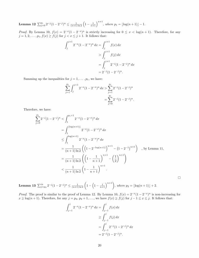
Lemma 12∑p1j=0 2−j(1− 2−j)n ≤ 1

(n+1) ln 2

(1− 1

n+1

)n+1

, where p1 = blog(n+ 1)c − 1.

Proof. By Lemma 10, f(x) = 2−x(1 − 2−x)n is strictly increasing for 0 ≤ x < log(n + 1). Therefore, for anyj = 1, 2, . . . , p1, f(x) ≥ f(j) for j < x ≤ j + 1. It follows that:∫ j+1

j

2−x(1− 2−x)n dx =∫ j+1

j

f(x) dx

>

∫ j+1

j

f(j) dx

=∫ j+1

j

2−j(1− 2−j)n dx

= 2−j(1− 2−j)n.

Summing up the inequalities for j = 1, . . . , p1, we have:

p1∑j=1

∫ j+1

j

2−x(1− 2−x)n dx >p1∑j=1

2−j(1− 2−j)n

=p1∑j=0

2−j(1− 2−j)n.

Therefore, we have:

p1∑j=0

2−j(1− 2−j)n <∫ p1+1

1

2−x(1− 2−x)n dx

=∫ blog(n+1)c

1

2−x(1− 2−x)n dx

≤∫ log(n+1)

1

2−x(1− 2−x)n dx

=1

(n+ 1) ln 2

((1− 2−log(n+1)

)n+1

−(1− 2−1

)n+1)

, by Lemma 11,

=1

(n+ 1) ln 2

((1− 1

n+ 1

)n+1

−(

12

)n+1)

<1

(n+ 1) ln 2

(1− 1

n+ 1

)n+1

.

Lemma 13∑∞j=p2

2−j(1− 2−j)n ≤ 1(n+1) ln 2

(1−

(1− 1

n+1

)n+1)

, where p2 = blog(n+ 1)c+ 2.

Proof. The proof is similar to the proof of Lemma 12. By Lemma 10, f(x) = 2−x(1− 2−x)n is non-increasing forx ≥ log(n+ 1). Therefore, for any j = p2, p2 + 1, . . . , we have f(x) ≥ f(j) for j − 1 ≤ x ≤ j. It follows that:∫ j

j−1

2−x(1− 2−x)n dx =∫ j

j−1

f(x) dx

≥∫ j

j−1

f(j) dx

=∫ j

j−1

2−j(1− 2−j)n dx

= 2−j(1− 2−j)n.

20

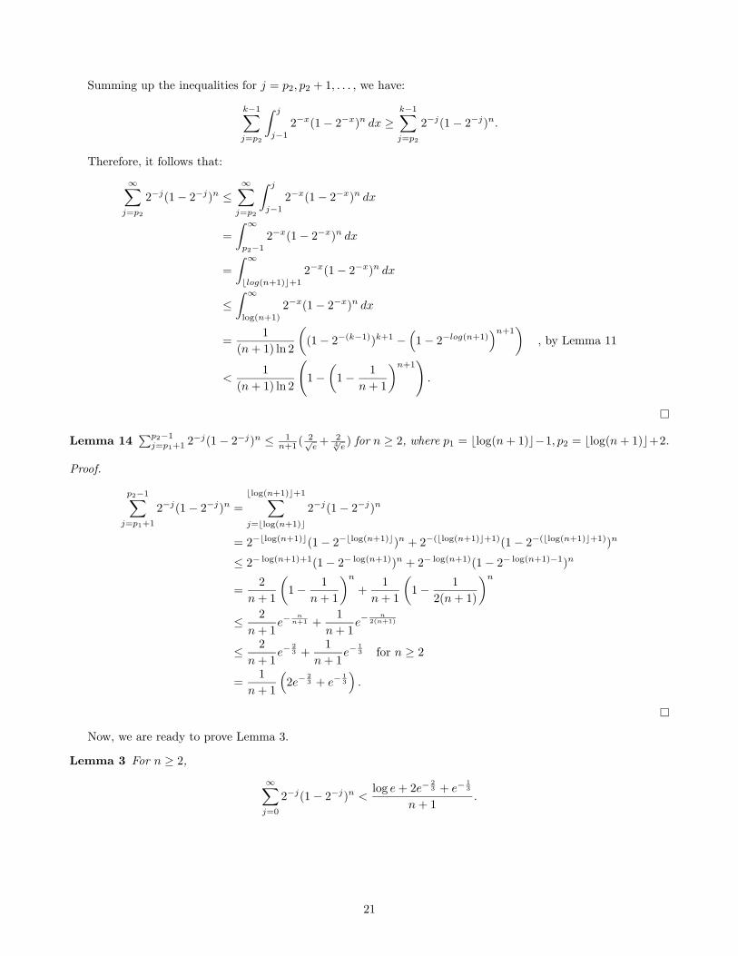
Summing up the inequalities for j = p2, p2 + 1, . . . , we have:

k−1∑j=p2

∫ j

j−1

2−x(1− 2−x)n dx ≥k−1∑j=p2

2−j(1− 2−j)n.

Therefore, it follows that:

∞∑j=p2

2−j(1− 2−j)n ≤∞∑j=p2

∫ j

j−1

2−x(1− 2−x)n dx

=∫ ∞p2−1

2−x(1− 2−x)n dx

=∫ ∞blog(n+1)c+1

2−x(1− 2−x)n dx

≤∫ ∞

log(n+1)

2−x(1− 2−x)n dx

=1

(n+ 1) ln 2

((1− 2−(k−1))k+1 −

(1− 2−log(n+1)

)n+1)

, by Lemma 11

<1

(n+ 1) ln 2

(1−

(1− 1

n+ 1

)n+1).

Lemma 14∑p2−1j=p1+1 2−j(1− 2−j)n ≤ 1

n+1 ( 2√e

+ 24√e ) for n ≥ 2, where p1 = blog(n+ 1)c−1, p2 = blog(n+ 1)c+2.

Proof.

p2−1∑j=p1+1

2−j(1− 2−j)n =blog(n+1)c+1∑j=blog(n+1)c

2−j(1− 2−j)n

= 2−blog(n+1)c(1− 2−blog(n+1)c)n + 2−(blog(n+1)c+1)(1− 2−(blog(n+1)c+1))n

≤ 2− log(n+1)+1(1− 2− log(n+1))n + 2− log(n+1)(1− 2− log(n+1)−1)n

=2

n+ 1

(1− 1

n+ 1

)n+

1n+ 1

(1− 1

2(n+ 1)

)n≤ 2n+ 1

e−nn+1 +

1n+ 1

e−n

2(n+1)

≤ 2n+ 1

e−23 +

1n+ 1

e−13 for n ≥ 2

=1

n+ 1

(2e−

23 + e−

13

).

Now, we are ready to prove Lemma 3.

Lemma 3 For n ≥ 2,

∞∑j=0

2−j(1− 2−j)n <log e+ 2e−

23 + e−

13

n+ 1.

21

Proof. Let p1 = blog(n+ 1)c − 1, p2 = blog(n+ 1)c+ 2.

∞∑0

2−j(1− 2−j)n =p1∑0

2−j(1− 2−j)n +p2−1∑p1+1

2−j(1− 2−j)n +∞∑p2

2−j(1− 2−j)n

≤ 1(n+ 1) ln 2

(1− 1

n+ 1

)n+1

+1

n+ 1

(2e−

23 + e−

13

)+

1(n+ 1) ln 2

(1−

(1− 1

n+ 1

)n+1)

=1

n+ 1

(1

ln 2+ 2e−

23 + e−

13

)

D.2 Proof of Lemma 4

In this section we will prove Lemma 4:

Lemma 4 For all n ≥ 2,

∞∑j=0

2−j(1− 2−j)n <log2 e+ 2e−

23 + e−

13

n+ 1.

Proof. The lemma can be proved by induction on n.

Base Case: The statement is true for n = 1, 2 and 3.

Inductive Case: Assume the statement is true for n− 1, where n ≥ 4. In other words,

∞∑j=0

1− (1− 2−j)n−2 ≤n−2∑j=1

C

j.

Then we prove the statement is true for n:

∞∑j=0

(1− (1− 2−j)n−1

)=∞∑j=0

(1− (1− 2−j)n−2(1− 2−j)

)=∞∑j=0

1− (1− 2−j)n−2 + 2−j(1− 2−j)n−2

≤n−2∑j=1

C

j+∞∑j=0

2−j(1− 2−j)n−2 , by inductive hypothesis

≤n−2∑j=1

C

j+

C

n− 1, by Lemma 3

=n−1∑j=1

C

j.

22