I

Faculty of Engineering

Department of Industrial Management and Logistics

Division of Production Management

REDUCING THE TIED UP CAPITAL

THROUGH INVESTIGATION OF PRODUCTION

POSTPONEMENT AND INVENTORY

Authors:

Lina Hedvall and Hanne Olsson

Supervisors:

Stig-Arne Mattsson, Division of Engineering and Logistics

The Financial Manager at the company

II

III

PREFACE This master thesis project is the final step to complete a Master of Science in Industrial

Engineering and Management at Lund University. The work started in early January

and proceeded to the end of May 2013. The project was carried out at the Department

of Industrial Management and Logistics at the Faculty of Engineering and a market

leading company within the process industry.

We would like to express our gratitude to a few people, who have supported us

throughout the work. Firstly, our supervisor at Lund University, Stig-Arne Mattsson for

his guidance and insightful feedback that helped us through the encountered difficulties.

His large experience in the field was very valuable. Furthermore, we would like to

thank the financial manager at the company, who also was our supervisor, both for

giving us the opportunity to write this thesis and also for helpful comments. There are

also other people at the company whom we would like to thank, for example the

production and product managers, the production planner and the manager for customer

relationship that have given us necessary data and also shared a bit of their vast

experience within the company. Without these people the purpose of this project would

have been almost impossible to fulfil

Due to anonymity reasons the name of the company and some sensible information

about the production process has been excluded or modified in the report. Careful

considerations have been made to not affect the outcome of this project or the reader´s

understanding of the case. The company is called Hyde AB.

IV

V

ABSTRACT

Title Reducing the tied up capital through investigation of production

postponement and inventory

Authors Lina Hedvall

Hanne Olsson

Supervisors Stig-Arne Mattsson

Financial manager at Hyde AB

Background

and purpose

The possibilities to reduce tied up capital have in most companies got

more attention in recent years, this since the lock up constrains a more

efficient use. The financial manager of Hyde AB, also the supervisor of

this master thesis, has long wondered about the possibilities to reduce the

total amount of tied up capital in the company by moving the goods in

the finished goods inventory to an intermediate storage in the production.

The products are then only finished at the arrival of a customer order.

The purpose of this master thesis project was to investigate the level of

tied up capital for Hyde AB in their production process and finished

goods inventory, in order to reduce unnecessary costs. This was to be

done with the strategies of inventory management and production

postponement. The purpose was also to present a well-executed

recommendation and to give clear and reasonable evidence for the

developed solution to Hyde AB.

Issues A complicating issue with inventory reduction at Hyde is that the

demand varies a lot from month to month, since the customers are few

and their orders large. Due to capacity constraints and recent growth

there has not been any focus on lowering the tied up capital as the

resources have been allocated to various expansion projects. This

expansion has also made Hyde AB to consciously increase the inventory

levels further to cope with future demand.

VI

Delimitations The company has several product families but only one is investigated in

this project. There are today two main warehouses at the production site,

the warehouse for raw material and the one for finished goods, where

only the latter was studied. There are other places within the company

where capital could be tied up as well, e.g. when products are being

processed in a machine, but this was not examined either.

The inventories were investigated by questioning its size and location.

The suggested changes might require capacity or technical adjustments in

the production; the feasibility or practicality of implementing those

changes in reality is not discussed in depth in this report.

Methodology At first, a literature study was carried out to find useable analytical tools

for the inventory review and to understand the possibilities and the

limitations with a postponement strategy. Company knowledge was

obtained through interviews, observations and from the information

systems. A simulation model was created to investigate if it was possible

to have an intermediate storage at different steps in the production.

Analysis In the first part of the analysis the main finding was the high inventory

level in the finished goods inventory. The level was far exceeding the

level set by Hyde themselves (safety stock + forecast) resulting in a high

cost of tied up capital. A review was also carried out to look upon if the

supposed inventory levels would have been sufficient to avoid stock outs

in 2012. It showed two stock-out occasions during the year, where it

would not have been possible to deliver to the customer in time. Due to

the high inventory levels this was no problem in reality.

Four different postponement scenarios were investigated where all or a

few product groups were placed in an intermediate storage. Only one of

the scenarios, to place product group YB before the mixing, was feasible

since the other scenarios resulted in longer production times than the

maximum time to shipping. This was true even though extensive

investments in production capacity were accounted for.

VII

Results and

conclusion

The purpose of the master thesis has been fulfilled; ways to reduce the

tied up capital have been recommended through general inventory

reduction (871 kSEK/year) and partly the use of a postponement strategy.

The most efficient way to reduce the inventory levels is to use a more

flexible production planning where smaller batches are enabled. Flexible

manufacturing is also required to make a postponement strategy possible.

Postponement of some products could be beneficial but the savings are

limited, hence postponement is only recommended if no additional

investments are required.

Keywords tied up capital, postponement, inventory management, safety stock,

finished goods inventory, risk-pool, demand variability

VIII

IX

TABLE OF CONTENT

1. Introduction .................................................................................................................. 1

1.1. Background ........................................................................................................... 1

1.2. Purpose .................................................................................................................. 2

1.3. Topic Background ................................................................................................. 2

1.4. Issues ..................................................................................................................... 3

1.5. Focus and Scope .................................................................................................... 3

1.6. Structure of the Report .......................................................................................... 4

2. Methodology ................................................................................................................ 5

2.1. Introduction ........................................................................................................... 5

2.2. Short Vocabulary ................................................................................................... 5

2.3. Ambition ................................................................................................................ 6

2.4. Type of Study ........................................................................................................ 7

2.5. Research Approach................................................................................................ 8

2.6. Types of Data Collection Methods ........................................................................ 8

2.7. Simulation ........................................................................................................... 10

2.8. Quality Assurance ............................................................................................... 11

3. Theoretical Framework .............................................................................................. 15

3.1. Definition of Logistics......................................................................................... 15

3.2. Inventory Management ........................................................................................ 15

3.3. Inventory Management Costs .............................................................................. 22

3.4. Push, Pull and Order Penetration Point ............................................................... 23

3.5. Postponement ...................................................................................................... 24

3.6. Additional Theories ............................................................................................. 32

4. Empirical Framework ................................................................................................. 33

4.1. Company Background ......................................................................................... 33

4.2. Production Process .............................................................................................. 34

4.3. Inventory Management ........................................................................................ 41

X

4.4. Products ............................................................................................................... 42

5. Analysis and Results .................................................................................................. 47

5.1. Inventory Management ........................................................................................ 47

5.2. Postponement ...................................................................................................... 68

6. Conclusion .................................................................................................................. 93

6.1. Inventory Levels .................................................................................................. 93

6. 2. Postponement ..................................................................................................... 95

6.3. Recommendations ............................................................................................... 97

6.4. Additional Observations ...................................................................................... 98

6.5. Criticism .............................................................................................................. 99

7. References ................................................................................................................ 101

8. Appendix ....................................................................................................................... i

8.1. Appendix 1: Shipped and Forecasted ..................................................................... i

8.2. Appendix 2: Inventory Levels .............................................................................vii

8.3. Appendix 3: Shipped & Inventory .................................................................... xiii

8.4. Appendix 4: Simulation Model .......................................................................... xix

8.5. Appendix 5: Correlation Coefficients .............................................................. xxiv

1

1. INTRODUCTION

The introduction aims to give the reader a general understanding of the content in this

project. Areas covered in this part are the background to the project, the purpose and

the issues to be solved. The focus is then further specified along with the scope. Finally

the report disposition is presented.

1.1. BACKGROUND This master thesis project was carried out at Hyde AB, a market-leading company

within their field. The company continuously develops new, more efficient, products

and expects a doubling in sales the coming five years. The production facility is already

today used close to its maximum and expansion projects will be carried out the coming

years. Within this expansion process a question was raised regarding how well the

production is managed today:

Is it possible to store semi-finished products in an intermediate step in the production

and by postponing1 the product differentiation

2 decrease the costs of tied up capital

3?

How would it affect production lead time, capacity and the total cost?

If the production is delayed, the demand uncertainty could be reduced and the safety

stock decreased. This would, in addition to the lower value of semi-finished products,

in turn reduce the cost of tied up capital. Also problems with the finished goods

inventory have been raised at Hyde, since the warehouse cannot hold what needs to be

stored today. Therefore the investigation was extended to also include the finished

goods inventory. To know appropriate inventory levels is also necessary to enable

decisions about postponement.

The target groups of this report are university students with basic knowledge in logistics

and statistics, as well as the case company Hyde AB. The report is written so that Hyde

would be able to implement the proposed recommendations and understand the

reasoning behind.

1 Postponement is the delaying of the product differentiation until demand is more certain

2 The action of distinguishing products from each other

3 Money is bonded in products and is locked from being used for other investments. The

potential profit from an alternative investment is named the cost of tied up capital.

2

1.2. PURPOSE The purpose of this master thesis project was to investigate the level of tied up capital at

Hyde AB in their finished goods inventory in order to reduce unnecessary costs. This

was to be done with the strategies of inventory management and production

postponement.

The purpose was also to present a well-executed recommendation and to give clear and

reasonable evidence for the developed solution to Hyde AB. The company presentation

was to be understandable and show a solution clear enough so that it could be

implemented by the company in the future.

1.3. TOPIC BACKGROUND Today, inventory management is of great importance in most companies. With concepts

such as “lean manufacturing” the question about what inventory to carry has been

emphasised. Lean manufacturing is a Japanese production philosophy with the aim to

reduce the seven types of wastes; overproduction, waiting, transporting, inappropriate

processing, unnecessary inventory, unnecessary/excess motion and defects.

Unnecessary inventory tends to hide problems in the production process and contributes

to long lead times, occupies floor space and delays problem identification. (McBride,

2003)

Inventory directly affects the return on assets (ROA) as well as the amount of working

capital available to do other more profitable investments. Inventories are valuable when

it comes to volatility in demand, when short lead times are expected and when there are

problems in the production. Disadvantages, apart from the tied up capital, are the need

of storage locations, material handling and IT-systems for tracking and control.

(Strategos, n.d.)

The importance of an inventory investigation in this case is clear, since the

characteristics of Hyde AB differ from the general assumptions in the main theory. The

small number of customers and their large orders make the demand from month to

month very volatile. This in combination with a long production lead time and high

utilization of machines makes it important to accurately plan orders and have the right

amount of inventory.

3

1.4. ISSUES It is important to have a suitable level of tied up capital in a company since holding

inventory is associated with an opportunity cost. The money tied up in products could

be used for other investments that generate a greater future profit for Hyde AB. Due to

the growth the last years there has not been any focus on decreasing the tied up capital.

Instead, resources have been allocated to expansion projects for increased production

capacity.

To be able to manage the volatile demand and still meet the desired service levels,4

Hyde is forced to have relatively high inventory levels. Furthermore, the production

today is not planned to be efficient from a tied up capital point of view but to achieve a

high utilisation rate. Large batch sizes are often used in the last production step, even if

the products are often not needed in those quantities. For example, even if there is a

forecasted demand of four tonnes, five tonnes are produced since that is the used batch

size. This further pushes the inventory levels up.

Today, almost all volume in Hyde is stored as individual products in the finished goods

inventory. To only store products as finished goods could result in high inventory

levels, since the demand of finished products varies more than the aggregated demand

of many semi-finished products. The production process of Hyde branches so that the

number of different products increases in each of the three final steps; this enables the

opportunity to aggregate the volatile demand in an intermediate buffer earlier in the

production.

These things combined have made the production and warehouse crowded, leading to a

situation where possibly higher levels of inventory than needed are used. If the

inventory levels are reduced it would also ease the material handling, since today

overflow inventory has to be transported to a separate storage location due to lack of

space.

1.5. FOCUS AND SCOPE The focus and scope in the project have been decided together with Hyde AB. In

inventory management, the safety and cycle stock levels of today were the main

interests. In postponement, the focus was on the possibilities to aggregate risks by

delaying production until a customer order arrives. The production time as well as the

amount of required additional production capacity was also investigated.

4 The percentage of orders that are delivered full in time to the customer

4

Hyde has several product families but only one of them is considered in this report.

Every product family has its own equipment and staff.

There are other places within the company where capital could be tied up as well, e.g.

in the raw material storage or when products are being processed in a machine, but this

is not examined in this thesis. The used products are returned from the customers and

then remanufactured to reduce the cost of raw material. The possible implications of

this for the production process were not considered.

The inventory was mainly investigated by questioning its size and location, in order to

find a suitable solution. The suggested changes might require capacity or technical

adjustments in the production; the feasibility or practicality of implementing for

example additional machinery is not discussed in depth in this report. Further on, no

technical solutions are presented for how to store the products or how material handling

should be organised in practice.

1.6. STRUCTURE OF THE REPORT This chapter, Introduction, aims to make the reader familiar with the reasons to why

this master thesis project has been carried out. This familiarisation includes the purpose,

an introduction to the topic, the issues and a discussion of where the focus will be. The

following chapter is about the methodology used and is more theoretical, with focus on

the science behind the research. Chapter three, Theoretical Framework, deals with

theories used in the area of inventory management and postponement.

In chapter four, Empirical Framework, the current situation at Hyde is discussed. It

includes the company background, the characteristics of the products and a description

of the production process and the finished goods inventory. Further, the chapter

Analysis is presented. In this chapter, the first part is about inventory management and

includes reviews of the safety stock and the inventory levels. The second part is about

postponement and how risk-pooling could reduce the cost of tied up capital. Finally, a

conclusion summarises the most important findings from the analysis and gives a

recommendation about future work.

5

2. METHODOLOGY

The purpose of the Methodology chapter is to show the approach to this project and the

methods that have been used to obtain knowledge and information. The findings

themselves are presented in chapter three, Theoretical Framework and chapter four,

Empirical Framework.

2.1. INTRODUCTION To introduce the reader to how this project has developed the chronological mile stones

are presented in a short-list below. Contact with personnel at and visits to Hyde AB

have taken place and literature has been researched throughout the project. The writing

process started early and the text was continuously developed as the project proceeded.

Initial visit to Hyde AB to get an overview of the company, its production and

the issue in concern. Further specification of the purpose, goals and scope.

Find the most suitable approach to the project (develop the methodology)

Literature study: mainly postponement and inventory management

Empiricism: investigation of production and demand characteristics

Simulation in ExtendSim: find the implications of a postponement strategy

Analysis of the results

Conclusion and recommendation

2.2. SHORT VOCABULARY To readers who are not familiar with the science of methodology, a short list of

common vocabulary is presented below. Knowledge of this vocabulary facilitates the

reading of this chapter.

Primary data is data collected directly by the researcher. (Andersen, 1998)

Secondary data is data collected by someone else than the researcher. (Andersen,

1998)

Qualitative methods are primarily descriptive and it is usually hard to do any

generalisations based on qualitative data. (Holme & Solvang, 1997) Hence, analytical

and statistical methods are rarely used in this context. The aim with a qualitative

6

method is mainly to understand a concept and not to find the cause of it. (Andersen,

1998)

Quantitative methods are analysis of quantitative data (numbers) with statistical and

analytical methods. The researcher chooses the approach to the problem, which is

usually stricter than in a qualitative analysis, leading to a greater control of what to

study. (Holme & Solvang, 1997) The aim is primarily to find the cause to an observed

issue and to enable predictions of future behaviour. (Andersen, 1998)

2.3. AMBITION The ambition level and the width of a project could be described through the steps of

knowledge in figure 1 below. Each step represents different depths of knowledge and

actions where the previous steps usually have to be fulfilled before entering the next.

(Nilsson, 2013) In this project the first four steps have been covered: the exploratory,

the descriptive, the explanatory and the predictive.

The exploratory step aims to give an understanding of the problem and an impression of

what is happening. Possible ways to do this is to be part of the system by observing it or

to map the process. (Wallén, 1996) In this project, the understanding was given from

several interviews, observations and thereafter a mapping of the process. Also an initial

seminar was held with people at key-functions to get a general understanding of the

issue and the context of the problem.

Figure 1: Steps of Knowledge

7

In the descriptive part the researcher has to understand the system in focus to be able to

describe it. Data can be collected and used to illustrate cause and effect between

different parts. The aim is to find the characteristics of the system. (Wallén, 1996) In

this part of the project, production data such as the production rate per hour and the

inventory levels was investigated.

The explanatory step aims to find the cause of the problem. The problem is identified

and described in the previous steps and this step aims to find the reason to why it has

occurred. (Wallén, 1996) In this project, the causes to the large amount of tied up

capital were understood through interviews with key personnel at Hyde AB,

observations and mapping/analysis of the production.

Predictive analysis uses the causes found in the explanatory step, to predict events and

behaviours in the future. To do this, analytical or statistical models are used. The aim

could be to predict the effect of a development project in a production process. (Nyce,

2007) In this project several analytical and statistical theories have been used to predict

the behaviour of the recommended implementation. These theories are primarily

covering postponement and inventory management, and are thoroughly described in

chapter three, Theoretical Framework.

2.4. TYPE OF STUDY A project could be approached in several different ways. To ensure the quality, regular

contact with the company and a good connection to existing theory has been

fundamental. In this project a combination of the two methods case study and action

research has been used.

The purpose of a case study is to describe an event or object in depth, and is especially

suitable if the phenomenon is hard to exclude from its surroundings. A case study

describes a specific case and does not necessarily have to be directly applicable in other

situations. The planning of a case study is flexible and could be changed and adapted

during the work. Some common investigation techniques are interviews, observations

and historical data analysis. (Höst, et al., 2006) All of these were used throughout the

work with this project as described later on.

Action research is sometimes described as a variant of a case study. This is because the

action research usually starts with the observation of a phenomenon in order to identify

or clarify the problem. One of the methods to do this observation is a case study.

Secondly, the researcher proposes a solution to the problem and suggests a way to

8

implement it in the company. (Höst, et al., 2006) In this project the first part, proposing

a solution, has been carried out. Since this project is carried out as a master thesis

project during one semester, the authors are not able to follow an eventual

implementation. The last part of the action research is the evaluation of the

implementation, which is not part of this project either. Of course, an in depth

discussion of the proposed solution is included in this report.

2.5. RESEARCH APPROACH The way theory and empiricism connects to each other could differ depending on the

chosen research approach. A real situation could be described and analysed from

existing theories in order to predict a behaviour (deduction), or general conclusions (or

theories) could be found from studying the reality (induction). (Wallén, 1996) In this

project, an abductive approach has been used. It could be seen as a mix between

deduction and induction and is characterised as a way where the effects of a problem

are known but there are many uncertainties about the causes. These causes are not

always possible to affect or change, but need to be identified so that a solution to the

problem could be found (Svennevig, n.d.).

When using the approach of abduction, in depth understanding and experience of the

area under investigation is necessary. The conclusions do not necessarily result in a

normative theory, but could be specific for the case in investigation. (Wallén, 1996) A

common way to work when using abduction is to first get a general understanding of

the situation, then search for available theories, followed by in depth empirical

investigation and ending up with a conclusion about the problem. (Svennevig, n.d.)

This is mainly the way the work within this project has been carried out.

2.6. TYPES OF DATA COLLECTION METHODS In this part the methods for data collection used in the project are described.

2.6.1. INTERVIEWS

There are three main types of interviews, structured, semi-structured and open. The

structured interview is close to a survey and is good to use for quantitative research.

The interviewer asks questions that all have fixed answers. An open interview gives the

opportunity to the interviewee to more freely talk about what she finds most interesting.

This can give important information but there is also a risk that some topics are

neglected. The semi-structured interview is a mix of the two others; there are both open

9

questions and fixed ones. When choosing interviewees for an open interview it is

important to find persons representing all stakeholders. (Höst, et al., 2006)

In this project, semi-structured, qualitative interviews have been a vital part of the data

collection. These were often conducted with key personnel within the company, such as

the production planner and product manager, but also production staff. The sharing of

experience from these people has been absolutely necessary to get an understanding of

the company, the production and the inventory system. Since an interview can be seen

as collection of secondary data the reliability and validity must be checked so that there

are no misunderstandings.

2.6.2. OBSERVATION

When studying a phenomenon, it is possible to take the position as an observer. The

observer can have different roles depending on the level of interaction with and

visibility to the studied object: complete participation, complete observer or somewhere

in between, as shown in table 1 below. The benefit with a “participant as observer” and

complete participant is that they receive all information, while the complete observer

can become somewhat excluded. If the observed people are aware of the observer, it

would likely affect their behaviour, but if the observer is hidden to them it is instead an

ethical dilemma. (Höst, et al., 2006)

In this project though, the role “observer as participant” was mainly used. Observations,

visible or through interviews, were made to get an overview of the warehouse and how

it functioned. There were no hidden observations made, and as far as possible there was

an aim to see the daily work as much as needed. Observations of the production process

Table 1: Possible roles as observer, (Gold, 1958)

Observational research roles

Complete

participant

Hidden observation, participation

Participant

as observer

Visible observation, participation

Observer as

participant

Usually interviews. No in-depth relationship

through a lengthy observation, no

participation

Complete

observer

Experimental design, no participation

10

itself were hard to carry out due to the long production time (some steps are today up to

72 hours) Primary data, of qualitative character, could be collected through

observations.

2.6.3. DATA COLLECTED FROM IT-RESOURCES

The company has an old-fashioned software solution for production planning where a

limited amount of information could be found; for example the times for different

production steps are saved only for a short period of time. The primary data used from

this system was mainly approximate times for different production steps.

Primary forecast data was manually gathered from Microsoft Excel-files sent from the

customer relationship manager to the production planner.

The WMS-system has been used to obtain primary data about inventory levels and

shipping rates. Unfortunately continuous data was not accessible, furthermore the data

received was not digital and had to be computerised by manually putting the values into

an Excel-file. This further limited the amount of data that could be analysed.

2.6.4. LITERATURE STUDY

A literature study is usually carried out in the initial part of a project to benefit from

previous work by others. The literature study is a way to familiarise the researcher with

the existing theory. The amount of initial research that is required depends on the

researcher’s previous knowledge and experience. (Andersen, 1998) Literature study is a

qualitative method where information from secondary data is gathered.

This project started with an extensive research among academic journals and textbooks

mainly in logistics and supply chain management. The research has primarily taken

place at the digital and physical libraries at Lund University, such as LibHub and the

University Library. Other tools have also been used, for example Libris and Google

scholar. Some of the textbooks were in Swedish which required careful translations of

terminology. To assist the translations Jan Olhager’s “Produktionslogistiklexikon” has

been used.

2.7. SIMULATION A simulation model was built up with the purpose of finding out how much production

capacity different postponement scenarios would need in order to handle the flow of

incoming orders. The model was created in the simulation software ExtendSim and can

be found in appendix 4.

11

A simulation model as a tool could be beneficial since a real life situation is imitated

and its behaviour can be predicted cheaply. One deficiency with simulation is the risk

of errors if the model is not correctly built or if faulty assumptions are made.

(Stillwater, 2003)

The task in this project was to see whether a future situation is feasible or not. This

meant that the simulated situation did not exist in reality, which resulted in difficulties

to validate the results. All results received through the simulations were carefully

checked to see whether they were plausible or not, but the results should be seen as

guidance only.

2.8. QUALITY ASSURANCE To ensure the quality of this project the concept of triangulation has been a key factor.

Triangulation means that the data is received and confirmed from more than one source.

It could, for example, be that different methods are used. (Höst, et al., 2006) In this

project, production data has been compared to interviews with the production manager

and the operational staff, and if there was any mismatch, further questions were asked

to find the reasons behind. In addition to that, the same questions have been asked to

several persons the same day.

Quality could be expressed by the measurements reliability and validity. Bullseye

analogy (see figure 2) is a common way to illustrate these measures. Every dot is a

sample of data (for example a production time), and the bullseye is what should be the

result. If the dots are scattered close together, as in the first picture, it shows that the

data collected is similar, thus the reliability is high. If the dots are spread evenly around

the bullseye, as in the second picture, it shows that the measured data represents what

the researcher was supposed to measure, the validity is high. The third picture shows a

perfect match, where both the reliability and validity is high. (New Mexico Department

of Health, 2012)

12

Figure 2: Bullseye analogy

Reliability could be seen as a way to describe how trustworthy collected data is in a

situation with random variations. (Höst, et al., 2006) A good measurement for

reliability is whether the same results would be found at a later data collection or not.

(Wallén, 1996) To ensure the reliability in this project, data from two years (2011 and

2012) was used to study the behaviour of the products and to detect extreme values.

In the qualitative analysis the main source of information was interviews with people at

key-functions in the company, who have had the possibility to check the data to ensure

that there were no misunderstandings. The slightly differing production times for the

products and the old fashioned production system made it harder to find reliable data, as

the products use the same machines. To achieve reliable production times, the times

from the production system were compared to numbers given from interviews with in

total five different people.

To check validity is to ensure that the right thing is measured. If the measure is not

valid, the analysis becomes inaccurate and could lead to significant costs to the

company. (Höst, et al., 2006) Bad validity gives a systematic error and could appear

when there are problems with for example measuring equipment. It is important to

ensure that not only the right thing is measured but also that nothing else is, for example

it is important to know if the setup time is included or not in the production time for a

certain step. To achieve this, it is important to have a good understanding of casual

relationships. (Wallén, 1996) In this project the validity has been safeguarded through

detailed interview questions to ensure that a full understanding has been obtained for all

data used in the analysis.

In this project there was a trade-off between reliability and validity, to ensure high

reliability data from several years had to be used. At the same time, the sales have

increased and the products have changed over years. Therefore it was not preferable to

13

use data from a longer time horizon. Two years of data, 2011 and 2012, was considered

to be valid and still give reliable results.

Representativeness is a measure of to what extent results can be transferred to other

companies and contexts. (Höst, et al., 2006) The representativeness of this project is

limited due to the somewhat special conditions. These conditions are carefully

described in chapter four, Empirical Framework, and a reader planning to do a similar

investigation in another company should carefully read those.

14

15

3. THEORETICAL FRAMEWORK

The purpose of this chapter is to describe the theories used in the project. It starts with

a definition of what logistics is, followed by the main parts: Inventory Management,

Inventory Management Costs, Push, Pull and Order Penetration Point and

Postponement. In the end some additional theories are presented briefly.

3.1. DEFINITION OF LOGISTICS To introduce this chapter the definition of logistics is first presented. The Council of

Supply Chain Management (former Council of Logistics Management) defines logistics

as following:

“Logistics is the part of the supply chain process that plans, implements, and controls

the efficient, effective flow and storage of goods, services, and related information from

point of origin to point of consumption in order to meet customers’ requirements.”

Another more simple way to describe the aims of logistics is the classical seven R’s.

“To ensure the availability of the right product, in the right quantity, in the right

condition, at the right place, at the right time, at the right cost, for the right customer.”

Logistics can be divided into three main functions; supply, production and distribution.

There are inventory between, and sometimes within, the functions. It is important to

have a high degree of integration between those functions to achieve high profitability.

If there is a lack of integration, each function will be optimised without regard to the

other parts in the chain. This will sub-optimise the company as a whole. The integration

has to include flow of both physical products and information. (Oskarsson, et al., 2006)

3.2. INVENTORY MANAGEMENT The main reason for inventory is to decouple different parts of a process from each

other in order to enable a more smooth production and distribution. In this part the

different types and functions of inventory are described, followed by an in depth

description about safety stock. Eventually theory about forecast accuracy and bias is

presented.

16

3.2.1. INVENTORY SYSTEMS

A production consists of different levels, where each level can have its own inventory.

Figure 3, 4 and 5 below show three different ways of how the inventory could be

managed. Normally it is wise to have the main part of the inventory at a point where

there are few items with a high and stable demand. (Axsäter, 2006)

The simplest type of inventory system is the serial structure (figure 3) where there is

one storage following on the other, and the path the product takes is predetermined and

the same for all variants. (Nilsson, 2006)

Another is the assembly structure (figure 4) where each level has at least one previous

step.

In the general structure (figure 5) each step can have one or more previous steps and

one or more subsequent steps. (Nilsson, 2006)

3.2.2. TYPES OF INVENTORY

There are several types of inventory and the most common are presented below.

Raw material inventory (RMI) is a way to reduce the dependence on timely and

accurate deliveries from suppliers. An idle production due to shortage of material is

Figure 3: Serial structure

Figure 4: Assembly structure

Figure 5: General structure

17

expensive and can cause lost sales. RMI will also enable the company to buy in bulk

and thereby reduce the cost. (Shan, u.d.)

Buffers are, in this report, referred to as small inventories in between production steps

to decouple sensitive parts of production. It could also be a way to ensure a high

utilisation rate of constraining equipment. All semi-finished goods (SFG), no longer

part of the RMI and not yet in the finished goods inventory, could be referred to as

work in process (WIP). Buffers could be seen as storages holding WIP. (Oskarsson, et

al., 2006)

Finished goods inventory (FGI) is a way to decouple the production and the sales

processes from each other. The FGI does also decrease the time for delivery to

customer, since finished products are ready for delivery. (Mattson & Jonsson, 2003)

3.2.3. FUNCTIONS OF INVENTORY

Within each of the inventory types described above the stored goods could have

different functions. The two most common is safety stock and cycle stock. The safety

stock is of significant importance in this project and is described in depth in the next

part (3.2.4). Also the cycle stock is of importance and could be defined as the inventory

on hand minus the safety stock. (Hartman, n.d.) Other inventory functions could be

speculation, e.g. the raw material price is expected to rise in the future, or season, e.g.

Christmas decorations could be produced throughout the year to decrease the capacity

need but are only sold around Christmas. Thus, they have to be stored in wait for the

right season.

3.2.4. SAFETY STOCK

The safety stock is a function of inventory with great importance; in this part, some

statistical concepts are explained followed by a description of how the service level

could be set and measured in a company.

The safety stock could be defined as a stock hold with the purpose of reducing the risk

of stock-outs. This is especially useful in the case of high demand variability, or

problems in production or supply. (Oskarsson, et al., 2006) The harder the demand and

supply is to forecast, the more safety stock is required. The amount of safety stock is

also dependent on the desired service level, as explained further. The service level is a

strategic decision for a company to take, if they wish to almost always be able to deliver

to customer straight from the stock, they will need a lot of safety stock which is costly.

(Chopra & Meindl, 2010)

18

Statistical measures

Statistical measures are of high importance when for example dimensioning a safety

stock. In this part, the normal distribution, standard deviation and coefficient of

variance are presented. If a sample of data is normally distributed it enables the use of

the most common methods to dimension a safety stock. The standard deviation could be

seen as a measure of variability, and if for example the demand is very volatile, the

standard deviation is large and more safety stock would be needed. The coefficient of

variance could be used to see if a sample of data could be approximated with a normal

distribution or not. It is also useful when comparing the variability of products with

dissimilar average demand.

The Normal distribution

When using the most common formulas to dimension safety stock, the normal

distribution is of great importance. If the sample follows a normal distribution, it is

characterised by a symmetric probability function, as seen in figure 6. Shortly

described, a probability function shows the probability of getting an observation in a

certain area. The total area below the curve is always one, representing a probability of

100%. Since the curve is symmetric it is possible to know how much that is within

boundaries of a certain number of standard deviations. If one standard deviation is

added on each side of the mean (μ +/- σ), 68,27% of the data is included, for two

standard deviations the same value is 95,45% and for three 99,73%. (Mattson &

Jonsson, 2003)

Figure 6: Normal distribution, (Answers, n.d.)

19

The Standard Deviation

A standard deviation (1) is a measure of variation.

It is calculated from the square root of the variance, V(X).The variance is calculated

from the expected value of the squared difference between the observation, represented

by the stochastic variable X, and the mean, μ. (Blom, et al., 2005)

When the standard deviation is used in practise, it is usually the standard deviation

during the lead time that is of importance. It could be expressed by the following

formula. (Chopra & Meindl, 2010)

Coefficient of Variance

The coefficient of variance (3) is a measure of the relative variation and is equal to the

quote between the standard deviation and the mean demand during a specific period of

time.

This measure could be used to see if a sample of data may be approximated with a

normal distribution. Mattsson (2003) has made a collection of different methods to find

when the normal distribution can be approximated. In that paper, for example

Schönsleben’s findings are presented: if the coefficient of variance is 0,4 or smaller an

Table 2: List of symbols

Symbols Explanation

σL standard deviation

during lead time

σi standard deviation in

time period i

L number of time periods

during lead time

20

approximation is valid. The coefficient of variance could also be useful in comparisons

of uncertainty between products with different average demand since the size of the

demand is taken into account.

Service level

When dimensioning a safety stock, the company must be aware of its desired service

level. The service level could be defined in a few different ways, where cycle service

level and demand fill rate are the most common. These are briefly described below.

Cycle service level (CSL): the fraction of replenishment cycles5 without stock-outs that

the company wishes to have. (Chopra & Meindl, 2010) In explicit, if there are 99 pieces

delivered correctly in one cycle and one miss, the whole period is considered a failure.

Demand fill rate (DFR): the desired fraction of demand to be served directly from

existing inventory. (Chopra & Meindl, 2010) In explicit, if 99 pieces are delivered

correctly and one fails, there are 99 successes and one fail.

When a method with CSL is used to dimension the safety stock, a larger stock is

required, for the same service level, than if a method with DFR is used. This comes

from the fact that CSL is harder to fulfil. (Oskarsson, et al., 2006)

Both CSL and DFR assume that only one piece is sold at a time, while in reality most

products are sold in greater quantities. This could increase the risk of shortage. Another

assumption is that the demand is normally distributed. In industry however, these two

measures of service level are very commonly used, even though the demand is not fully

normally distributed. How to mathematically dimension safety stock from the service

level is not further explained in this report.

Measurement of Service Level

The methods to determine service level described above are not used to measure the

actual service level. The most commonly used measures are order fill rate and order line

fill rate.

Order fill rate (OFR): the fraction of orders that can be served straight with products

in inventory (Chopra & Meindl, 2010) Order fill rate is referred to as an external metric,

telling something about how customers experience the availability of products. (Gibson

& Novack, 2008)

5 A replenishment cycle is the time between two subsequent replenishment deliveries to a

warehouse.

21

Order line fill rate (OLFR): the fraction of order lines that can be served straight with

products in inventory. This is an internal metric which is a signal about how well the

inventory levels are set for certain products. (Gibson & Novack, 2008)

3.2.5. FORECAST ACCURACY AND BIAS

It is important to measure the accuracy of the forecast and to find eventual bias. This

since the production is planned after these forecasts and the safety stocks are set in

accordance to the outcome.

Forecast bias is the systematic error found by calculating the average error between

forecast and sales. Hence, the bias tells if the forecast is continuously too large or too

small. A good forecast should not have any bias. (Mattson & Jonsson, 2003) The

accuracy is measured by finding the standard deviation of the forecast error. If this

standard deviation is large, the accuracy of the forecasts is generally low, and a larger

safety stock is required. The importance of the standard deviation is stressed in

Thomopoulos’ example where he shows that one percentage increase in the coefficient

of variance for forecast errors results in 2,18% more safety stock to reach the same

service level. (Thomopoulos, 2005)

Ritzman and King (1993) discuss how forecast errors affect the inventory levels and

customer service in a manufacturing company. Two components of the forecast error

are examined; the bias of the forecast and the standard deviation of the forecast errors

(forecast accuracy). The bias is proven to be much more important than the forecast

accuracy. What is also shown in their study is that the production lot size is an even

greater driver than the forecast to reach the correct inventory levels. (Ritzman & King,

1993)

Another important factor while evaluating forecast is to find which demand that is

“normal” and which is due to a large and non-reoccurring order or a demand peak due

to a shortage in an earlier period. Peaks of this type should not be included during the

evaluation since isolated occasions would have unacceptably high influence on the

results. (Mattson & Jonsson, 2003)

An alternative and very simple way to measure the forecast accuracy is through the

percentage error.

22

3.3. INVENTORY MANAGEMENT COSTS This part introduces the reader to some of the most important costs regarded in

inventory management. First economies of scale and scope are elaborated followed by a

presentation and discussion about the trade-off between inventory and setup costs.

3.3.1. ECONOMIES OF SCALE AND SCOPE

Economies of scale and scope are of importance when large volumes of or types of

products could be produced in a factory. The greatest difference between the concepts

is that scale refers to the volume of one product while scope is more concerning the

number of different products. (The Economist, 2008)

Economies of scale states that increasing the volume of one product produced would

decrease the individual cost of each and every product. (The Economist, 2008) The

benefit from economies of scale appears since the fixed cost associated with a

procedure is shared among the volume passing through. Hence the absorption cost of

each and every product decreases. (Heakal, 2009)

Economies of scope, on the other hand, say that producing a wide variety of products

would decrease the total costs since some vital functions like marketing and finance are

shared. The benefits could also come from cross-selling, meaning that additional

products or services could be sold to a customer. (The Economist, 2008)

3.3.2. INVENTORY AND SET UP COSTS

The costs mainly associated with inventory are the holding and inventory carrying cost.

The holding cost is about the cost to run a warehouse and do not change when adding or

removing a unit, while the inventory carrying costs mostly depend on the additional

costs for each and every stock keeping unit (SKU)6. (Oskarsson, et al., 2006)

Holding cost includes the costs to run a warehouse such as: ownership, daily

operations, employees, equipment and transports within the warehouse. These costs

usually change between certain intervals of volume. (Oskarsson, et al., 2006)

Inventory carrying cost includes the cost for the stored products in the warehouse

such as tied up capital and risk. The cost for risk includes obsolescence, waste, damage

and insurance. The cost for tied up capital can be seen as the opportunity cost for not

investing the money in a better way. If the money is freed up it can be used somewhere

else and the return from those investments is seen as the cost for tied up capital. The

6 A SKU is a warehousing unit that is stored and accounted for separately from other items.

(WebFinance Inc., n.d.)

23

return rate achieved from an investment is often called the internal rate of return (IRR).

The inventory carrying cost is often directly proportional to the amount of goods stored.

(Oskarsson, et al., 2006)

To calculate the inventory carrying cost, the inventory carrying charge (ICCh) could be

used.

The Setup cost includes the costs associated with the preparation of a machine for

production of a new batch of products. It could include cost for administration, to

change tools, moving materials to the machine or some initial testing of the output.

Since the machine is idle during the setup time there is also an opportunity cost of not

being able to produce. (Averkamp, n.d.) The setup cost is closely linked to economies

of scale; if the batch volume increases, the setup cost per product decreases.

3.4. PUSH, PULL AND ORDER PENETRATION POINT All manufacturing processes could be divided into two stages depending on if they are

carried out in anticipation for or in response to a customer order; the push and pull

process. When a pull process is executed, the customer demand is known with

certainty; it could be seen as a reactive process. The push process on the other hand is

supported by forecasts and could be seen as speculative. (Chopra & Meindl, 2010) A

push/pull system could be consisting of an entire pull or push process, or a hybrid

structure combining the two phases. (Rafiei & Rabbani, 2011)

The push/pull interface is located somewhere in the main process. This is the point

where the pull and push phases are separated from each other and is called the order

penetration point (OPP). It is from this point in the production that a specific product is

allocated to a certain customer. Even though the pull phase is carried out with certain

demand, some uncertainty is still present because of inventory and capacity decisions in

the push phase. (Chopra & Meindl, 2010)

24

In table 3 different classifications of a push/pull system are shown. Depending on

where the OPP is located a production system could be seen as of type make-to-stock

(MTS), make-to-order (MTO) or a hybrid MTS/MTO. (Rafiei & Rabbani, 2011)

Benefits with the push phase are high capacity utilization and the simplicity of the

coordination between actors in the process. The disadvantages are high throughput time

and tied up capital because of inventory. The latter is of course dependent on the

forecast accuracy. There is a great need for planning and the process is very production

oriented. (Oskarsson, et al., 2006)

The benefits with the pull phase are low amount of tied up capital and that the only

inventory used is to cater for small differences in demand. Disadvantages are that the

flow could become sensible to disturbances in demand. (Oskarsson, et al., 2006)

3.5. POSTPONEMENT Postponement is a suitable theory to use in situations where there is a need to combine

especially two factors: high production volume and customization. The method

suggests the company to take decisions about completion of generic semi-finished

goods (SFG) when more information of the demand is known, in other words after the

OPP. (Chopra & Meindl, 2010)

3.5.1. LOCATION OF ORDER PENETRATION POINT AND DIFFERENTIATION POINT

Figure 7 shows six different ways in which the OPP and differentiation point (DP)

could be located. All figures except from “a” illustrate some kind of postponement. The

options “a” and “b” show an entire push and pull system respectively. In “a”, the DP is

before the start of production while the OPP is when all the products are finished. When

the company receives an order, the product is taken directly from stock. The production

Table 3: Order penetration points

Structure Procurement Process Delivery

Make-to-

Order

OPP

Hybrid

MTO/MTS

OPP

Make-to-

Stock

OPP

25

is planned completely from forecasts. In “b”, all production is executed in response to

an arrived customer order. As the OPP is located in the beginning of the production,

there are great possibilities for product differentiation. (Wong, et al., 2009)

In “c” and “d”, the generic SFG are produced to stock in order to aggregate the demand.

In “c” the OPP is in the “customized product inventory”, while the DP is in the “generic

component inventory”. The demand is not known in the DP, but it is probably more

certain than in the beginning of the process, and since there is still just one generic SFG

there is potential for risk-pooling. In “d”, the DP and OPP are both located in the

“generic component inventory”. This means that the first phase of the process is of push

type and the second of pull type. The demand for the finalized products is aggregated in

the “generic component inventory”, also here contributing to risk-pooling. (Wong, et

al., 2009)

Figure “e” and “f” could be seen as a combination of the previous figures. Here all

generic SFG are produced through the same flow, but they are not stored in any

intermediate step. In “e” some of the benefits of postponement are achieved since the

DP is partly delayed, leading to more certain demand. The OPP is still in the

“customised product inventory” meaning that all products are sold from stock. In “f”,

all products use the same generic path, even though a customer order has already

arrived before production starts. In the “generic component inventory” the products are

differentiated, but there is no delay. (Wong, et al., 2009)

26

Due to production postponement, risk-pooling is possible since the aggregated demand

of the generic SFG before differentiation is less volatile than the individual demand of

each and every end product. If the forecast is based on the aggregate demand, it could

lead to higher accuracy. (Chopra & Meindl, 2010)

Figure 7: Possible positioning of OPP and DP

27

3.5.2. HOW TO AGGREGATE DEMAND

When the order penetration point is moved backwards and the production decision is

postponed, the generic SFG represents the new uncertainty. The uncertainty is

measured in standard deviations.

The demand of the postponed products is the same as the sum of the individual

demands, see formula 7 below. (Chopra & Meindl, 2010)

To get the new standard deviation, the formulas 8 and 9 below are used. The

uncertainty could be decreased due to risk-pooling. (Chopra & Meindl, 2010)

Table 4: List of symbols

Symbols Explanation

Dagg aggregated demand

Di demand for product i

σagg aggregated standard

deviation

σi standard deviation

for product i

X number of products

in aggregated group

agg

the aggregated

demand correlation

i,j

correlation between

products i and j

28

Key factors that positively affect the benefits of aggregation are: if the products show

high demand variability, they are negatively correlated7, more products are being

postponed and most importantly if they share the generic SFG. (Graman & Magazine,

2006) Another thing that is important is the demand between the products which has to

be quite similar to make use of the benefits of risk-pooling. (Chopra & Meindl, 2010)

Below is an example of how the aggregation of demand is very dependent on if one

product has a much larger variability than the other.

When aggregating standard deviations, their squares are first added together, and

then the new standard deviation is set to be the square root of that sum. The square

of 20 is 400, and the square of 10 is 100. Hence, one product with a standard

deviation of 20 and three of 0 will give the same aggregated standard deviation as

four products with a standard deviation of 10. This makes postponement more

beneficial if the standard deviations are similar for all products.

3.5.3. FACTORS FOR BENEFICIAL POSTPONEMENT

Three different main aspects can be identified to influence the benefits of

postponement: market factors, process factors and product factors. (Swaminathan &

Lee, 2003)

Market factors concern the customer demand and expectations of service level.

Parameters included here are demand variability, correlation in demand between

different products, lead time and service requirements. (Swaminathan & Lee, 2003)

Process factors regard the manufacturing and distribution process that the company

can control themselves. Factors included here are the sequence of operations performed,

capacity, resources, whether the product is made-to-order or made-to-stock, network of

the supply chain (manufacturing and distribution sites) and how much and where

inventories are stored. (Swaminathan & Lee, 2003)

Product factors relates to the design of the products. It concerns the level of

standardization of the products, how much it would cost to standardize and to what

degree the final products could be substituted by each other. (Swaminathan & Lee,

2003)

The benefit from postponement comes from the improved matching of demand and

supply. But there is also a cost associated since the production cost usually increases

due to the changed routines. It is important to thoughtfully consider the decision so that

7 When the total sales of one product go up, the sales of the other product go down.

29

Chart 1: Postponement strategies

the expected benefit exceeds the cost. (Chopra & Meindl, 2010) The activities after

OPP have to be smoothly carried out in order to achieve efficient postponement.

(Young, et al., 2004)

3.5.4. TYPES OF POSTPONEMENT

Postponement could be carried out in different ways, for example labelling, packaging,

assembly, manufacturing and time postponement. Labelling postponement refers to the

case when only the attachment of the label remains when the customer order arrives. In

packaging postponement the product is finished but not fully packaged before OPP.

Assembly and manufacturing postponement refers to the case when the manufacturing

or assembly is not finished before a customer order arrives. Time postponement is when

products are not shipped until an order has arrived from a specific market.

(Swaminathan & Lee, 2003)

A general rule presented by Young et al. (2004), seen in chart 1, is that the lower the

uncertainty of the product is, the later in the supply chain can the point of

differentiation be located. If the demand is very uncertain it is advisable to locate the

point of differentiation early in the process, as in the point of purchasing or product

development. In this stage no physical inventory exists. If the commonality of the

products is very low it could be better to postpone in the logistics (time postponement)

or in the purchasing stages than in production and product development.

30

In production postponement there are two different main types of changes to be made

when adapting to a postponement strategy, the ones related to the processes and those

related to the products. In process postponement the focus is on re-sequencing and

standardizing the processes so that they could be used for different types of products.

Product postponement refers to the work of developing commonalities between

different products. (Swaminathan & Lee, 2003)

3.5.5. POSSIBLE ISSUES WITH POSTPONEMENT

A problem that could arise during the implementation of postponement is lack of

cooperation and understanding between different functions in a company. To solve this,

a cross-functional team representing all relevant functions in the company could be

created to keep a holistic view of the changes. A tendency is that in older companies

with strong local autonomy it is generally harder to make major changes in the

processes compared to newly developed ones. (Graman & Magazine, 2006)

3.5.6. HYBRID POSTPONEMENT

One way of postponement is the hybrid structure, where only some of the material is

postponed. The basic idea is that the incremental benefits of postponement diminish

beyond a certain point, and that only the positive effect of postponement should be

delayed. Chart 2 shows an example of how much the inventory could be reduced in

response to different amounts of postponement of the expected demand. In this

example, the benefit of postponement diminishes when about 30 % of the expected

demand is postponed. (Graman & Magazine, 2006)

Chart 2: Hybrid postponement, the line indicates how the initial gains from postponing the first

20% of inventory is great but then the benefit is quickly decreasing

31

3.5.7. POSTPONEMENT WITH MULTIPLE POINTS OF DIFFERENTIATION

A system with multiple points of differentiation is seen in figure 8, where T1, T2 and T3

are lead times and the circles are points of differentiation. In the first stage, T1, all

variants are generic before they are transformed into different product families at

differentiation point one. After the second differentiation point the actual products are

formed. Early postponement could then be defined as changing T1 to T1+1 and T2 to T2

-1. Thus, products will spend more time before differentiation point one than after.

Alike, late postponement is defined as changing T2 to T2+1 and T3 to T3 -1.

The demand for the system is assumed to be independent, normally distributed and

identical during time periods, and the lead times, T1, T2 and T3, are the same for every

product. The system is assumed to use periodic review with a base stock policy8. The

level of inventory at each circle, in figure 8 below, has to be so high that the storages

could be seen as independent and decoupled from each other. In an environment

fulfilling all these assumptions, the following is true: (Swaminathan & Lee, 2003)

If T1 > T2 > T3, then both early and late postponement are beneficial.

If T2 >> T1,T3, then late postponement is beneficial.

If T2 << T1,T3, then early postponement is beneficial.

8 Base stock policy is also known as the policy of periodic review. Thus, a production order is

placed after inspection of inventory levels, if the levels are under a set base stock. The

inspections are done periodically.

Figure 8: Multiple points of differentiation

32

3.6. ADDITIONAL THEORIES In this part, some additional theories are presented.

3.6.1. THEORY OF CONSTRAINTS

Theory of constraints is a way to identify the bottleneck (the constraining factor) in a

production. The constraining factor prevents the production to obtain its goal or develop

in a desired direction. (Rahman, 1998) It is the part of the production that has the lowest

throughput; hence it sets the production rate for the whole system. (Sullivan, 1998)

3.6.2. NET PRESENT VALUE

The net present value (NPV) is used to find if an investment is profitable or not. It

could be very useful as it accounts for time value of money. To use the formula the

company must be aware of its desired pay-back time, the internal rate of return and the

cash flows.

The formula for NPV is seen below (10). When adding the desired values on the

parameters, the formula gives a value larger than zero if the investment is profitable and

oppositely, a negative value is the investment is not profitable. (Jan, n.d.) The symbols

used are explained in table 5.

Table 5: List of symbols

Symbols Explanation

n payback time

i internal rate of

return

R net cash flow

IC initial cost

y year 1, 2,...,n

33

4. EMPIRICAL FRAMEWORK

The empirical framework describes the company today. The chapter begins with the

general characteristics, followed by a description of the production process, inventory

management and the products. The aim with this chapter is to make the reader familiar

with Hyde AB in order to better understand the analysis.

4.1. COMPANY BACKGROUND Today Hyde AB is the market leader within the product segment in consideration and

has been so for several decades. The characteristics of the company are as shown in this

part quite unique, and no similar studies regarding postponement or inventory

management have been found.

The company has a limited number of customers, today about 160. The production

facility in Sweden ships to either international customers or to a sales warehouse in the

United States. In this project, the U.S. warehouse (and its clients) is considered as one

customer, leading to a total of about 116 customers. Due to the nature of the product,

the orders are large, similar in size for a specific customer and arrive at certain

intervals. These intervals are about 8-12 months and the average order size is about 2,5

tonnes. In 2012, the production got 144 orders, on an average twelve per month.

The relationships with the customers are often long term and the customer service is of

great importance. This is one of Hyde’s most important competitive advantages in

combination with the offering of superior quality. Therefore late deliveries are not

acceptable, even if it would incur high costs to avoid them. Today the service level is

not measured, but the personnel responsible for customer orders cannot remember a

single late order during their time in the company. If the service level was measured,

order fill rate and not order line fill rate would have to be used since incomplete orders

are of no interest to the customers. However, as mentioned in 3.2.4 order line fill rate

can be interesting to evaluate the inventory levels.

In this project, one specific product family is regarded, involving 23 different products.

They all originate from the same material, and this material is in the production process

continuously modified into different products. In this report, the unfinished products are

referred to as semi-finished goods (SFG). Of the 23 different products, six are pure and

34

17 mixed. How these appear is described further, but the mixes are pure products

diluted with additional material.

4.2. PRODUCTION PROCESS This section presents the production process at Hyde AB. It consists of two parts, here

called A and B, which both have several steps. The two parts are decoupled from each

other with a buffer, but almost all storage takes place after the production in the

finished goods inventory. There is a graphical presentation of the production process in

figure 9 on next page.

To ensure the anonymity of Hyde AB the production steps are not described in depth,

but it should not affect the reader’s understanding of the report as a whole. Due to the

nature of the products the production needs to follow the steps in the current order.

Ten people work five-shift in the production, which results in production 24 hours a day

seven days a week. In addition to this there are one person employed to take care of the

finished goods storage and several office-workers. In total, the company has about 90

employees.

4.2.1. PART A

Part A of the process has two steps. All SFG follows the same production steps and is

made out of the same raw material; thus the SFG stored in the end of part A is of the

same type for all products.

The steps in part A is now described in more detail. The first step is preparation of the

raw material. There are two machines that produce independently from each other.

When the preparation is finished, the machines empty themselves, one at a time, and the

SFG goes into the next process step called drying. When the SFG dries, it is

continuously transported away to the buffer where it is stored until needed in part B.

The maximum capacity for this storage is 12,5 tonnes.

To empty one container with 245 kg of prepared raw material on to the dryer takes 2,5-

2,9 hours. This gives a production rate of between 84-98 kg/hour, which is also the

production rate from the dryer to the buffer. Part A needs to be closed for eight hours

every ninth day. This represents a downtime of about 4 %, leading to an average

production rate of 81- 94 kg/hour.

35

Figure 9: Production process. Square figures indicate a value-adding step, triangles indicate

storage or waiting. The labels below indicate how many product groups there are at each point.

36

4.2.2. PART B

Part B is given the main focus in this report. It has four different steps and there are

three points of differentiation: the shaping, the oven and the mixing, graphically shown

in figure 9. Different SFG groups are continuously formed in the process and a scheme

of the connections between the final 23 products is shown in figure 10 below. In this

figure it is possible to see which products that origin from the same group and where

they start to differ. To understand the rest of the report this figure should be studied

carefully since the introduced denotations are extensively used.

Granulation When the SFG is needed, it is taken from the buffer to the granulation. Two substances

are added and the material is granulated. This step is the same for all products. The

granulation process including transport takes 2-3 hours.

Figure 10: Product scheme, at each differentiation point the number of product groups

increases. In the end, there are 23 products.

37

Shaping Shaping is the first point of differentiation. There are six shaping machines, all of which

can work independently from each other. The machines have different capacity, the two

largest always produce product group X or Z, while the four smaller produce X or Y.

With today’s production planning the maximum production rate is between 118 kg/hour

(product Z in the two biggest machines and X in the others) and 161 kg/hour (X in the

larger machines, Y in the smaller). Z is produced with a rate that is 10% lower than

product X.

The shaping machines require extensive maintenance. Most importantly, every 300

hours (12,5 days) the whole step is shut down for 3-4 days. There are ongoing

investigations to find alternatives where the machines are closed at different times to

enable partial production in the step at all times. The other type of maintenance is daily,

every eighth hour all machines need to shut down for 10-15 minutes to be cleaned.

Those two types of planned standstills represent about 24% of the total time. The

average production rate, including those standstills, is 89-122 kg/hour.

After the shaping, the SFG wait in small buffers that open and release material every

fourth hour for product group Y and every fifth hour for X and Z. Only one buffer

releases at a time, meaning that if another buffer is open, some extra waiting may be

necessary before the SFG are transferred into one out of three load carriers. Every load

carrier can take 725 kg and there is only one at a time that can be filled up.

Oven At the third production step in part B, the load carriers with SFG are placed in the

ovens. At the time of this writing there are five ovens working independently, during

the late spring of 2013 one of those will be replaced with a new one with double

capacity. At the moment each oven can take one load carrier (725 kg) for every cycle.

The cycle time is approximately 41 hours, slightly depending on the product group and

oven. The time span is 38-42 hours with an emphasis on the longer times. Shorter oven

time is not possible to achieve by decreasing the amount of goods in each load carrier.

Instead, the quality cannot be guaranteed if the load carriers are not filled.

The ovens produce in three different temperatures, giving three different characteristics.

All product groups before the ovens, X, Y and Z, are not given all these three

characteristics. The theoretical maximum of different product groups after this step is

nine, but in reality only six different groups are created. See the product scheme in

figure 10 above for more details.

38

In the oven, water evaporates and after this step the load carrier holds 625 kg. So if the

production rates before the ovens should be compared with the ones after, this reduction

needs to be considered.

Mixing and Packaging The last step in the production process is the mixing and packaging. The mixing is an

adding of different quantities of inexpensive, extra material. From the six product

groups entering9 the mixing/packaging station, 23 products are made. Of these 23, six

are pure and do not receive the additional material. This step can take maximally 5 000

kg (eight load carriers) and just one product group at a time. From one batch in the

oven, all end products of the same product group (see figure 10) can be created. I.e. if

YB enters the mixing machine, YB100 (pure), YB50, YB55 and so on, can be created

from the same load carrier. Further on in this report, the added material is not taken into

consideration in the calculations, if the opposite is not clearly stated.

The setup time can be divided into two parts, firstly, 10 minutes to change the settings

on the mixing machine when a new product group is to be mixed and then another 5-10

minutes to empty one load carrier. Naturally, this time is dependent on the number of

load carriers mixed. Thus, today the setup-time is about one hour. In addition to this,

time for the operator to get to the machine must be added.

The final packaging contains 50 kg product each, and there are 12 packages on one

pallet. Hence, a pallet consists of 600 kg.

The production time in the mixing/packaging is dependent on the characteristics of the

finished product. For a pure product that has no additional material it takes 1250

seconds to fill up a package. For mixed products each package requires less packing

time (900 seconds) but as more packages are needed for the same amount of SFG

entering, the total time is longer. Additional time of 30 minutes is needed in between

each pallet. Production rates for all variants can be seen in table 6.

9 XA, XB, XC, YA, YB and ZA.

39

After this step there are six pure products as well as 17 mixed products.

4.2.3. SUMMARY

The production rates and capacities for the different production steps are summarised in

table 7 below. The weight reduction in the oven is considered and the steps before are

reduced accordingly.

Table 7: Production capacity for all steps

Production step Capacity Part A 70-81 kg/hour Buffer (maximum

capacity) 10 750 kg

Part B

Transportation and

granulation 2-3 hours

Shaping 77-105 kg/hour

Small buffers Releases material

every 4-5 hours

Oven 76 kg/hour

Mixing and packaging 98-125 kg/hour

Table 6: Production rates in the

mixing/packaging

Product Production

rate (kg/h)

XA100, XB100,

XC100, YA100,

YB100 125

ZA100 116 XA70, XC70,

YA70, YB70 116

YB65 112 XA60, XC60,

YA60, YB60 108

XA55, YA55,

YB55 104

XA50, XC50,

YA50, YB50 101

YB45 98

40

4.2.4. PRODUCTION PLANNING

Hyde has two different procedures for production. The more frequently sold products

(representing 99,2% of the total volume and 57% of the products) are produced in

response to forecasts. This procedure is named make-to-stock (MTS). The order

penetration point (OPP) is then located in the finished goods inventory. Rarely sold

products are only produced in response to customer orders and are in Hyde AB referred

to as make-to-order (MTO). For those products the OPP is located in the buffer in the

beginning of part B. According to the terminology used by Rafiei & Rabbani (2011) in

3.4, they should be referred to as hybrid MTS/MTO-products. To not confuse the

readers from Hyde, the notaion of MTO is used here as well.

Hyde plans the MTS-production from monthly forecasts. The production planner is

given a document where the forecasted demand for the four coming months is

presented. After receiving this data the production planner checks the current inventory

levels. The month where the inventory level minus the forecasted demand falls below

the safety stock a production order is placed. The production planner is responsible for

the detailed planning, where he sets the production sequence and priority in intervals of

20 days. If an urgent order arrives, the prioritisation is flexible and rearrangements

could occur.

The forecasts originate from the expected sales, which are then adjusted by the product

manager according to prior experience. The forecast accuracy is today not measured

specifically for each product, but only for the product family as a whole, on a yearly

basis. The accuracy measured in percentage error (3.2.5) is then about 10%, which is

considered accurate.

Hyde does not have a set delivery time; instead the aim is to always deliver when the

customer wants the products. The time between order placement and desired delivery

date varies a lot for different customers depending on, among others, the method of

payment. The shortest time a customer can expect, from an order is placed until the

products are shipped, is one week. Within this week, one to two days are required to

pack the order. If the order contains at least one MTO product, the delivery time is

about three weeks as there is no use of having just a few of the products earlier. The

production planner has to confirm all orders that include MTO products before the

customer gets to know the exact delivery date. In average, an order contains 3,5 order

lines.

41

4.3. INVENTORY MANAGEMENT This part discusses the inventory management at Hyde today. The inventory in the

finished goods inventory (FGI) could broadly be divided into two different categories

based on functions.

The first function is the safety stock, which fills the purpose of protection against

uncertainties, as discussed in the section 3.2.4. In Hyde the total safety stock of all

products are set as a twelfth (representing one month) of the total forecasted demand

during a year. The total forecast for 2012 was 600 tonnes, leading to a safety stock of

50 tonnes. The division of safety stock between the products is decided by experience.

The safety stock levels during 2012 are shown in table 8 below.

The second function of the inventory is the cycle stock. The inventory in this function

originates from the forecasted demand the upcoming month plus excess inbound

inventory. This value could vary significantly between months. In table 8 the average

inventory level during 2012 is shown together with the targeted inventory level. The

average inventory level is found as a mean of the inventory level in the beginning of

every month, as no continuous data was available. The targeted level, on the other hand,

shows the level of inventory the company aims to have. It is twice the safety stock and

represents two months forecasted demand, where one month is the safety stock and one

month the forecast.

Since the production is based on forecasts, there are months when the shipping is less

than expected and there is a surplus of goods left in the finished goods inventory. If the

sales/forecasts the upcoming month are less than the surplus, an aggregation of

inventory will occur. If it is the opposite way, that the sales/forecasts next month are

larger than the surplus, the production planner will have to produce the difference

between the surplus and the forecast. The surplus is in this report referred to as excess

inbound inventory.

Today the warehouse is crowded and all goods cannot fit, therefore an additional

warehouse has to be used. This second warehouse is placed several hundred meters

from the production plant.

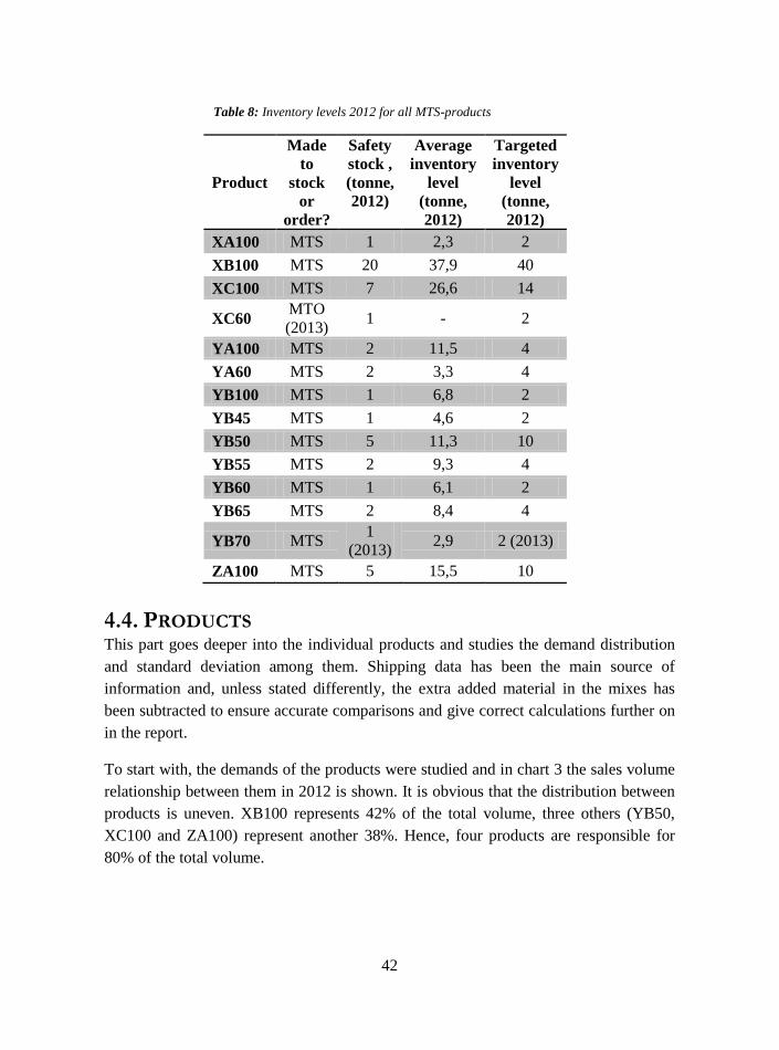
42

4.4. PRODUCTS This part goes deeper into the individual products and studies the demand distribution

and standard deviation among them. Shipping data has been the main source of

information and, unless stated differently, the extra added material in the mixes has

been subtracted to ensure accurate comparisons and give correct calculations further on

in the report.

To start with, the demands of the products were studied and in chart 3 the sales volume

relationship between them in 2012 is shown. It is obvious that the distribution between

products is uneven. XB100 represents 42% of the total volume, three others (YB50,

XC100 and ZA100) represent another 38%. Hence, four products are responsible for

80% of the total volume.

Table 8: Inventory levels 2012 for all MTS-products

Product

Made

to

stock

or

order?

Safety

stock ,

(tonne,

2012)

Average

inventory

level

(tonne,

2012)

Targeted

inventory

level

(tonne,

2012)

XA100 MTS 1 2,3 2

XB100 MTS 20 37,9 40

XC100 MTS 7 26,6 14

XC60 MTO

(2013) 1 - 2

YA100 MTS 2 11,5 4

YA60 MTS 2 3,3 4

YB100 MTS 1 6,8 2

YB45 MTS 1 4,6 2

YB50 MTS 5 11,3 10

YB55 MTS 2 9,3 4

YB60 MTS 1 6,1 2

YB65 MTS 2 8,4 4

YB70 MTS 1

(2013) 2,9 2 (2013)

ZA100 MTS 5 15,5 10

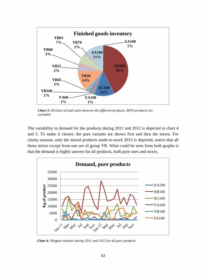
43

Chart 3: Division of total sales between the different products. MTO-products are

excluded.

Chart 4: Shipped volumes during 2011 and 2012 for all pure products

The variability in demand for the products during 2011 and 2012 is depicted in chart 4

and 5. To make it clearer, the pure variants are shown first and then the mixes. For

clarity reasons, only the mixed products made-to-stock 2013 is depicted, notice that all

those mixes except from one are of group YB. What could be seen from both graphs is

that the demand is highly uneven for all products, both pure ones and mixes.

XA100

1%

XB100

42%

XC100

13%

YA100

1%

YA60

1%

YB100

2%

YB45

2%

YB50

14%

YB55

2%

YB60

3%

YB65

7% YB70

2%

ZA100

11%

Finished goods inventory

0

5000

10000

15000

20000

25000

30000

35000

Kg

of

pro

du

ct

Demand, pure products

XA100

XB100

XC100

YA100

YB100

ZA100

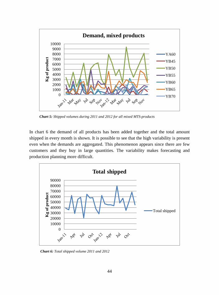
44

Chart 5: Shipped volumes during 2011 and 2012 for all mixed MTS-products

Chart 6: Total shipped volume 2011 and 2012

In chart 6 the demand of all products has been added together and the total amount

shipped in every month is shown. It is possible to see that the high variability is present

even when the demands are aggregated. This phenomenon appears since there are few

customers and they buy in large quantities. The variability makes forecasting and

production planning more difficult.

0

1000

2000

3000

4000

5000

6000

7000

8000

9000

10000 K

g o

f p

rod

uct

Demand, mixed products

YA60

YB45

YB50

YB55

YB60

YB65

YB70

0

10000

20000

30000

40000

50000

60000

70000

80000

90000

Kg

of

pro

du

ct

Total shipped

Total shipped

45

In table 9 the average demand and the standard deviation of the monthly demands are

presented for all products aggregated. The average amount of goods shipped per month

in 2011 was 36 tonnes and in 2012, 40 tonnes. This corresponds to an increase of about

11% from the previous year. The standard deviation on the other hand decreased from

11,8 to 9,2 which is about 22%.

Table 9: Average demand and

standard deviation on a monthly basis

2011 and 2012

Shipping 2011 2012

Average

demand 36,4 40,3

Standard

deviation 11,8 9,2

46

47

5. ANALYSIS AND RESULTS

In this chapter, the demand uncertainty of the finished goods is first examined in detail.

The current inventory levels are then questioned, including an in depth analysis of the

safety stock level and risk of stock out. Further on, there is a thorough analysis into

whether a postponement strategy would be profitable or not; the factors of customer

delivery time and production capacity have been of major importance.

5.1. INVENTORY MANAGEMENT In this part the finished products are analysed. First the demand uncertainties are

identified through a review of demand variability and the forecast errors. Thereafter, a

thorough investigation of the overall inventory levels of today and how they could be

reduced is presented. This is followed by the development of a method to determine

safety stock levels in a company where the normal distribution is not applicable. These

developed safety stock levels are then compared to the ones used in Hyde today.

This is partly done to see whether there are any possibilities to reduce the amount of

tied up capital in the finished goods inventory. The other reason is the importance of

good understanding of the inventories in order to appropriately decide whether a

postponement strategy is useful or not.

5.1.1. DEMAND UNCERTAINTY

To start with, two methods have been used in order to analyse the demand uncertainty

of Hyde AB, demand variability and forecast accuracy. This was done in an early stage

and the implications of the uncertainties have been regarded throughout the project. To

explain the two measurements, demand variability shows how the demand fluctuates in

comparison to the average demand, while the forecast accuracy is a measure of how

well the forecasts follow the registered demand. The standard deviation of the demand

and the standard deviation of the forecast error are the measurements used to

characterise these uncertainties. When investigating the forecasts, the bias was also

studied to find potential systematic forecast errors.

Forecast Bias and Accuracy If the forecasts have good accuracy, it indirectly affects the needed safety stock levels

in a positive way. This is because the error between the demand and the forecast is

generally small and the risk of shortage decreases. When finding the forecast accuracy,

it is important to remove the bias from the forecast errors to give a correct result.

48

The forecast bias on the other hand does affect both the cycle and safety stocks. If there

is a positive bias (too much forecasted), the cycle stock would become larger than what

is actually sold. The extra inventory would in a way act as an additional safety stock. If

the safety stock for the next period is dimensioned from those levels without removing

the bias, the new safety stock would, if there is no bias next year, become too small

since the risks for shortages have been very small during the year. If there is a negative

bias, the cycle stock could become too low, leading to a risky situation where the safety

stock is insufficient to cope with the systematically too low forecasts. On the contrary

to positive bias the negative bias results in too large safety stocks the next period if it is

not removed.

In table 10 below the bias for 2011/2012, the standard deviation of the forecast error

and the coefficient of variance are presented for each and every product. The bias was

found from the average of the forecast errors. The standard deviation was found from

the unbiased forecast errors, in explicit the forecast error minus the bias for that year.

Interesting to notice is for example XB100 which showed a clear positive bias in 2011.

On the contrary the following year the bias was negative. That aggravates the creation

of an accurate safety stock. In this case, if the safety stock was set after the results in

Table 10: Forecast bias 2011 and 2012, standard deviation for the two years combined and lastly

the coefficient of variance

Product Bias 2011

(tonne)

Bias 2012

(tonne)

Standard

deviation (tonne)

Coefficient of

variance

XA100 -0,1 -0,1 0,8 3,05

XB100 4,7 -4,2 6,6 0,43

XC100 4 2,7 4,7 0,85

YA100 0,8 0,5 1,9 1,49

YA60 0,5 -0,1 0,8 1,83

YB100 -0,1 0,9 2 2,81

YB45 0,4 1 0,8 1,50

YB50 0,4 -0,4 2,2 0,47

YB55 0,1 -0,1 1,6 1,22

YB60 -0,1 0,2 1,1 1,24

YB65 0,5 -0,1 1,1 0,60

YB70 - -0,3 0,7 0,94

ZA100 -0,5 2,4 3,4 0,83

49

2011 there could have appeared several shortages during 2012 if the bias from 2011

was not removed. YB50 shows a similar pattern as XB100, but was not spanning in as

wide range. ZA100 shows the reversed behaviour from XB100, and XC100 has a

considerably large positive bias in both 2011 and 2012.

To compare the forecast accuracy of different variants with each other the coefficient of

variance was used. In this case it is a measure of the ratio between the standard

deviation of the forecast error and the average demand. A low coefficient of variance is

usually achieved for variants where it is easier to do the forecast. The products that

show the least variability in comparison to their average demand are XB100 and YB50.

The values are based on data from both 2011 and 2012.

In charts 7 and 8 the forecast is compared to the shipping for XB100 and YB50, the two

products with the highest sales. What could be seen is that the forecast for XB100 is too

high in 2011, but too small in 2012. The forecast for YB50, on the other hand, was

continuously more even and the bias was smaller.

For XB100 and YB50, the accuracy is good and the coefficient of variance is the lowest

of all products. The reason to the low coefficient of variance is their very large demand.

In general, products with higher demand got lower coefficients of variance. Charts like

7 and 8 can be found for all products in appendix 1. In all those charts, the weight of the

additional material is included for the mixed products. This does not affect the result, as

the extra material is included in both the values for shipping and forecast.

50

Demand Variability The demand variability is a measure of the volatility in demand for a product. There are

especially two reasons to why demand variability is studied in this report. It is an

important factor in the context of inventory reduction as greater variability inhibits the

easiness of making accurate forecasts, which in turn leads to a requirement of larger

0

5000

10000

15000

20000

25000

kg

of

pro

du

ct

Shipped & Forecasted YB50

Forecasted

Shipped

0

5000

10000

15000

20000

25000

30000

35000

40000 k

g o

f p

rod

uct

Shipped & Forecasted XB100

Forecast

Shipped

Chart 8: Shipped volumes and forecasted demand for YB50

Chart 7: Shipped volumes and forecasted demand for XB100

51

Chart 9: Demand for XB100 and YB55. The top line represents XB100 while the one below

is YB55.

safety stock. The variability is also crucial when deciding whether postponement is

profitable or not, as it affects the risk-pooling possibilities.

The demand variability is measured as the standard deviation of the monthly demands

for each product. As discussed in section 4.4 the demand at Hyde is highly volatile. In

chart 9 the shipped demands for popular XB100 (ave. 15,4 tonnes, st. dev. 5,7) and the

less popular YB55 (ave. 1,3 tonnes, st. dev. 1,2) are shown.

Standard deviations are hard to use when comparing different products since the

measure does not include the average demand. Thus, a product with high demand

appears as more volatile. To enable comparison, the coefficient of variance is presented

in chart 10. This measure includes both average demand and standard deviation. What

could be seen is that the greater the average demand is the lower coefficient of variance.

This in turn means that products with greater average demand have smaller standard

deviation in comparison with their demand than products with low demand. To interpret

this into safety stock; a product with high demand would require a smaller share of its

demand as safety stock than a product with low demand.

0

5000

10000

15000

20000

25000

30000

35000

kg

of

pro

du

ct

Demand for XB100 and YB55

XB100

YB55

52

It is of great use to know whether the demand follows a normal distribution or not.

According to Schönsleben (3.2.4) the coefficient of variance has to be less than 0,4 to

make the approximation of normal distribution possible. This is the case for XB100 and

YB50 with a coefficient of variance of 0,3 and 0,4 respectively. For the other products

though, this estimation is not valid and the normal distribution can generally not be

used at Hyde.

5.1.2. THE INVENTORIES TODAY

Now when the main demand uncertainties are identified, the inventories of today are

further elaborated around. This part discusses the behaviour and level of the inventory,

as well as how it could be improved from a tied up capital point of view. In the

graphical illustrations, the features of XB100 and one other characteristic product is

shown. XB100 is always used since it represents such a large share of the total

demand. Information about all the other products can be found in chapter eight,

Appendix.

Inventory Levels in Response to Safety Stock and Target Level The first part to be studied is the inventory level in comparison to target level and safety

stock during the last two years (2011, 2012). The two charts 11 and 12 are displayed

below to show the inventory levels of XB100 and YB65.

0,0

0,5

1,0

1,5

2,0

2,5

0 5000 10000 15000 20000

Coef

fici

ent

of

va

ria

nce

Average demand 2012 (kg)

Coefficient of Variance in relation to

average demand

Product

Trend line

Chart 10: Coefficient of variance for all products. The trend line is an exponential

function set by Microsoft Excel.

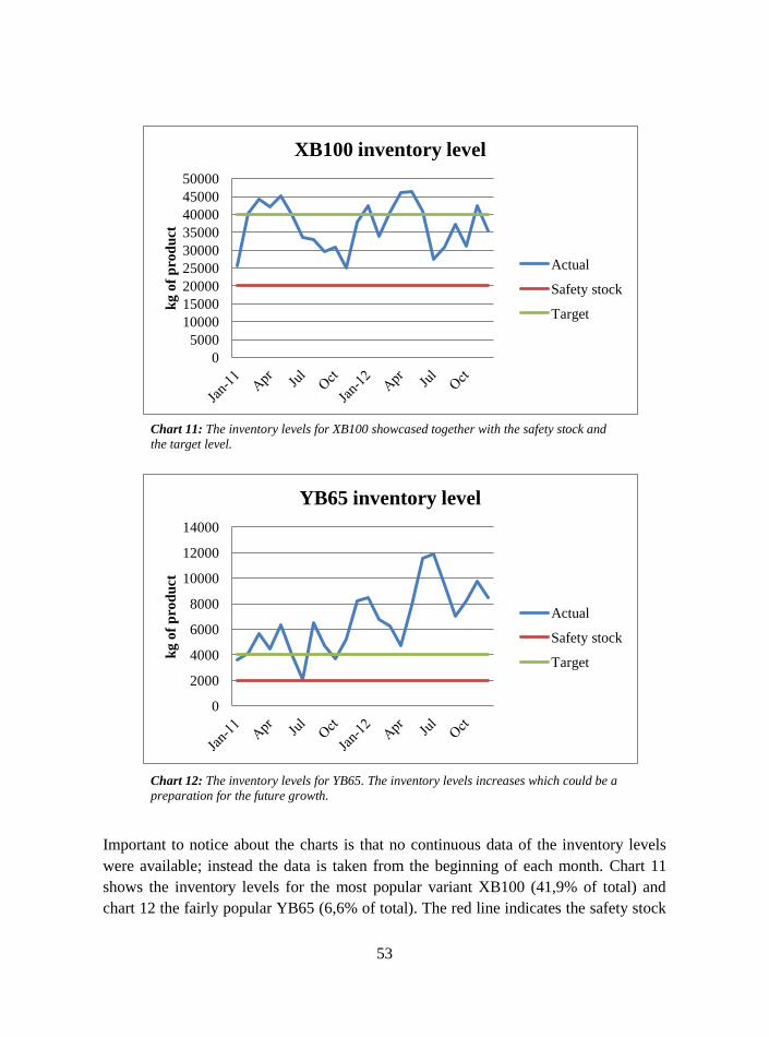
53

Important to notice about the charts is that no continuous data of the inventory levels

were available; instead the data is taken from the beginning of each month. Chart 11

shows the inventory levels for the most popular variant XB100 (41,9% of total) and

chart 12 the fairly popular YB65 (6,6% of total). The red line indicates the safety stock

0

2000

4000

6000

8000

10000

12000

14000

kg

of

pro

du

ct

YB65 inventory level

Actual

Safety stock

Target

0

5000

10000

15000

20000

25000

30000

35000

40000

45000

50000 k

g o

f p

rod

uct

XB100 inventory level

Actual

Safety stock

Target

Chart 11: The inventory levels for XB100 showcased together with the safety stock and

the target level.

Chart 12: The inventory levels for YB65. The inventory levels increases which could be a

preparation for the future growth.

54

level while the green line is the targeted level. The targeted level is the double safety

stock and is in Hyde said to be the goal level of inventory. The safety stock is updated a

few times per year, but only one report concerning 2011 and 2012 was reachable; hence

the straight red lines. The lack of information does probably not affect the results

significantly since the changes of safety stock levels have been limited between 2009

and 2013, from where other reports could be found.

In chart 11 the inventory level follows the target level pretty good, and during 2011 and

2012, there was no need to use the safety stock. A more common case for Hyde is

shown in chart 12; the target level is reached three times during two years of time but

most of the time the inventory level is much higher. For all the 13 products being

produced to stock, three never go below the target level and nine of them never use the

safety stock at all. For many of the products reaching the target level, a great share has

an inventory level that just slightly goes below it. For the interested reader, the charts

showing safety stock and target level for the other products are shown in appendix 2.

The target level is important as it is the level Hyde aims to have. This measure though

is fairly inaccurate as it does not change if the forecast for one month is very large or

very small. As Hyde has a very volatile demand, the result could turn out to be

misleading. Because of this, the safety stock plus the monthly forecast is considered to

be the desired inventory level in the remaining parts of this project. To not mix it with

the target level, it is referred to as the supposed inventory level.

Inventory Levels in Response to Demand

Now, when it is shown that the inventory levels during the last two years have been

high in comparison to the target/safety stock level, the analysis continues to study how

large the inventories have been in relation to the shipped demand. In this section the

implication of large inventory levels on the cost of tied up capital is also discussed.

Chart 13 and 14 below show the inventory levels and shipping rates for XB100 and

YB60 during 2011 and 2012. In the charts, the material added to the mixes is included.

The actual inventory level is usually much higher than shipped values; in July 2012

YB60 has the largest shipment during the two years and there are still 6,3 tonnes left in

inventory. The lowest inventory level for YB60 is 2,7 tonne, which includes the safety

stock set by Hyde of 1,8 tonne. See appendix 3 for charts of the other products.

55

Chart 14: Shipped values and inventory levels in the beginning of each month for XB60

0

2000

4000

6000

8000

10000

12000

14000

16000

kg

of

pro

du

ct

Shipped & Actual inventory level YB60

Shipped

Actual

To be able to find the implications of a large inventory level on the cost of tied up

capital, it is firstly important to find what the inventory level should have been, i.e. the

supposed average inventory level. It is calculated with formula 11 and 12 below. To

first get the supposed total stock for each product, the safety stock, forecast and excess

inbound inventory in the beginning of every month 2012 was added together (11). To

then get the average inventory level, the total stock every month was subtracted by half

0

5000

10000

15000

20000

25000

30000

35000

40000

45000

50000 k

g o

f p

rod

uct

Shipped & Actual inventory level XB100

Shipped

Actual

Chart 13: Shipped values and inventory levels in the beginning of each month for XB100

56

the shipped value that month. The given numbers for all months were summed together

and then split by 12 to get the supposed average inventory level. (12) This measure

assumes that everything that is forecasted for a month is in the finished goods inventory

in the beginning of the month and that there is an even outtake. In reality, the forecasted

demand would partly be produced during the month as well. Hence, the true inventory

levels would be lower.

This value is then compared to the actual average inventory level. This number is

estimated by summing the actual stock in the beginning of each month and divided by

12. (13) This assumes that during a year, the actual value in the beginning of a month

is, on the whole, representative for the average. This might not always be the case, but

during a year the shipments should be spread relatively even throughout the months,

making this an acceptable simplification.

In table 12 below, potential savings 2012 of having more control of the inventories are

shown (including weight and value of extra material). The first column is the supposed

average inventory level, while the second column is the actual average inventory level.

Table 11: List of symbols

Symbols Explanation

AI

actual average inventory

level

SI

supposed average

inventory level

x month 1,2,3...12

SS safety stock

F forecasted

EII excess inbound inventory

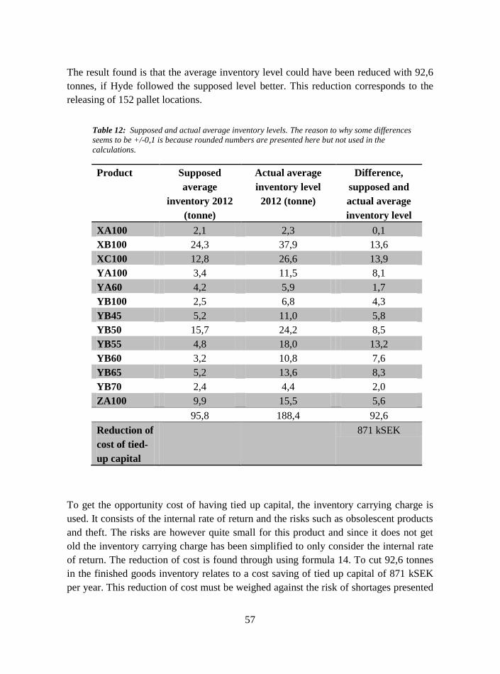
57

The result found is that the average inventory level could have been reduced with 92,6

tonnes, if Hyde followed the supposed level better. This reduction corresponds to the

releasing of 152 pallet locations.

To get the opportunity cost of having tied up capital, the inventory carrying charge is

used. It consists of the internal rate of return and the risks such as obsolescent products

and theft. The risks are however quite small for this product and since it does not get

old the inventory carrying charge has been simplified to only consider the internal rate

of return. The reduction of cost is found through using formula 14. To cut 92,6 tonnes

in the finished goods inventory relates to a cost saving of tied up capital of 871 kSEK

per year. This reduction of cost must be weighed against the risk of shortages presented

Table 12: Supposed and actual average inventory levels. The reason to why some differences

seems to be +/-0,1 is because rounded numbers are presented here but not used in the

calculations.

Product Supposed

average

inventory 2012

(tonne)

Actual average

inventory level

2012 (tonne)

Difference,

supposed and

actual average

inventory level

XA100 2,1 2,3 0,1

XB100 24,3 37,9 13,6

XC100 12,8 26,6 13,9

YA100 3,4 11,5 8,1

YA60 4,2 5,9 1,7

YB100 2,5 6,8 4,3

YB45 5,2 11,0 5,8

YB50 15,7 24,2 8,5

YB55 4,8 18,0 13,2

YB60 3,2 10,8 7,6

YB65 5,2 13,6 8,3

YB70 2,4 4,4 2,0

ZA100 9,9 15,5 5,6

95,8 188,4 92,6

Reduction of

cost of tied-

up capital

871 kSEK

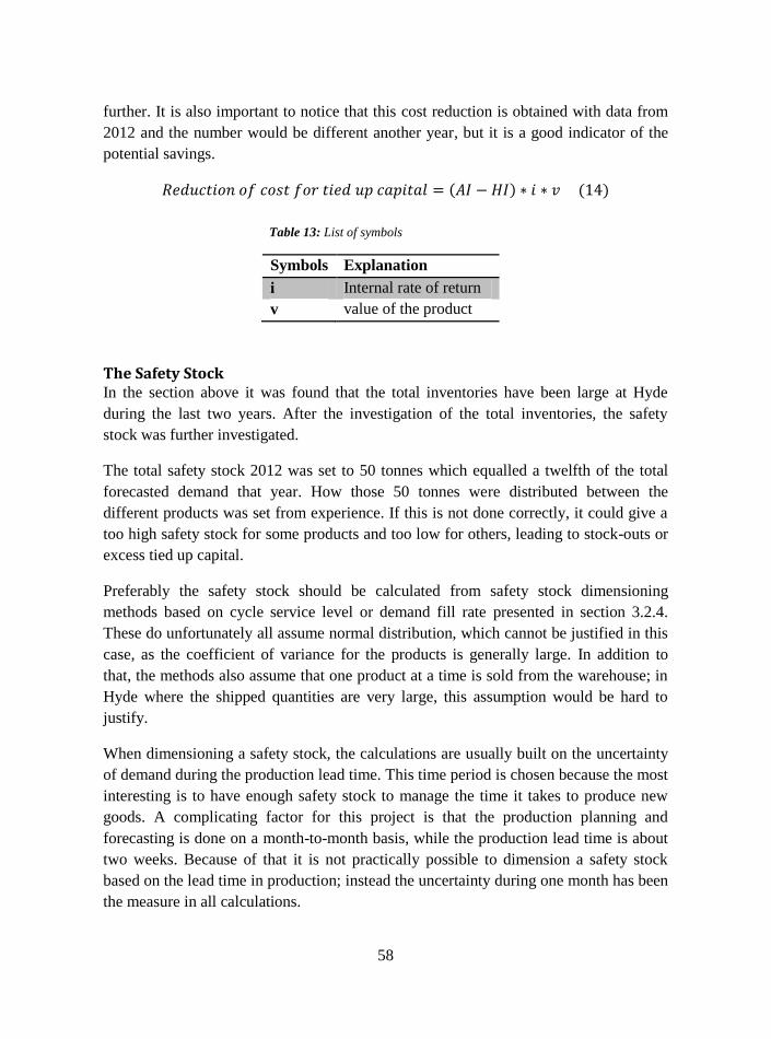
58

further. It is also important to notice that this cost reduction is obtained with data from

2012 and the number would be different another year, but it is a good indicator of the

potential savings.

The Safety Stock In the section above it was found that the total inventories have been large at Hyde

during the last two years. After the investigation of the total inventories, the safety

stock was further investigated.

The total safety stock 2012 was set to 50 tonnes which equalled a twelfth of the total

forecasted demand that year. How those 50 tonnes were distributed between the

different products was set from experience. If this is not done correctly, it could give a

too high safety stock for some products and too low for others, leading to stock-outs or

excess tied up capital.

Preferably the safety stock should be calculated from safety stock dimensioning

methods based on cycle service level or demand fill rate presented in section 3.2.4.

These do unfortunately all assume normal distribution, which cannot be justified in this

case, as the coefficient of variance for the products is generally large. In addition to

that, the methods also assume that one product at a time is sold from the warehouse; in

Hyde where the shipped quantities are very large, this assumption would be hard to

justify.

When dimensioning a safety stock, the calculations are usually built on the uncertainty

of demand during the production lead time. This time period is chosen because the most

interesting is to have enough safety stock to manage the time it takes to produce new

goods. A complicating factor for this project is that the production planning and

forecasting is done on a month-to-month basis, while the production lead time is about

two weeks. Because of that it is not practically possible to dimension a safety stock

based on the lead time in production; instead the uncertainty during one month has been

the measure in all calculations.

Table 13: List of symbols

Symbols Explanation

i Internal rate of return

v value of the product

59

Due to the complicating issue of not being able to approximate the demand of the

products with a normal distribution, a method was developed to find an appropriate

safety stock. It is now described in detail. The method is firstly described graphically

and later also analytically to ensure a clear understanding of the procedure. Observed

values from 2011 were used to find the safety stock level for 2012.

The size of a dimensioned safety stock is usually dependent on the variability of

demand, as a more fluctuating demand makes it harder to do accurate forecasts. In the

developed method, the size of the standard deviation is not directly used, but to give the

reader an understanding of the variability in demand for different products 2011, the

average demand (15) and standard deviation of demand (16) per month for make-to-

stock products are shown in table 14.

60

Table 14: Average demand and standard

deviation for all MTS-products

Product Average

demand

2011

Standard

deviation

2011

XA100 0,3 0,6

XB100 14 5,8

XC100 6,1 3,9

YA100 2,2 2,5

YA60 0,9 0,6

YB100 0,6 1,8

YB45 0,2 0,4

YB50 3,7 1,9

YB55 1,7 1,5

YB60 0,8 1

YB65 1,2 0,8

YB70 - -

ZA100 3,7 3,4

If the demand is normally distributed and if three standard deviations of demand are

kept as safety stock, demand is met in 99,73 % of the months (3.2.4) . When the normal

distribution does not work, it is possible to originate from the empirical distributions of

each and every product instead. The developed method starts by checking how much

inventory, in addition to forecast and excess inbound inventory, was needed to cover all

demand during a longer period of time. How this value turns out is dependent on the

size of the forecast errors and the amount of excess inbound inventory.

Firstly, the method is described graphically in chart 15 shown below. The dashed line

represents the shipped quantity and the solid lines the total stock with different amounts

of safety stock. In this illustrative chart the safety stock is set to three different levels

called safety stock one, two or three. With safety stock one there is a larger shortage in

May with 1,3 tonnes, with stock three there is a risk of excess inventory. With number

two on the other hand the shipping curve is almost equal in May. YB60 is by that

regarded to need a safety stock of a size close to safety stock two. When using the

method in this project, the needed safety stock was firstly set so that the total stock line

61

touched the shipped line. The bias was also considered and last some add-on stock was

given to especially important products. This is explained in detail further. Chart 15

includes the additional mixing material.

Chart 15: Depiction of the procedure to find accurate safety stocks.

The procedure is now described analytically in a short list.

The forecasts 2011 were firstly corrected to not include any bias.

is the unknown value of the safety stock.

Total stock was calculated for every month 2011 by:

Total stock was compared to the shipped values (2011) in every month.

The value of was minimised to a point where the total stock did not fall

below the shipped values in any month, but equalled in one.

The safety stock for 2012 was firstly set to .

0

1000

2000

3000

4000

5000

6000

7000

8000

9000

10000

Kg

of

pro

du

ct

YB60 inventory levels and shipping

Total stock 1

Total stock 2

Total stock 3

Shipped

62

Lastly, the safety stock levels were finalised by multiplying the value in the

prior point with an add-on that depended on how often the product was ordered.

This add-on is discussed further.

As the size of the largest forecast error is a main factor in the described method, it is

important that the forecast is not biased. How a biased forecast would affect the

developed safety stock is elaborated around in part 5.1.5.

If, for example, the studied time period is not as long as wished for, it could affect the

reliability of the method. A good way to handle this risk is to divide the products into

groups depending on their importance. Then more important products could be given an

add-on of a certain percentage. The criteria to use and the percentage to add have to

depend on the specific situation.

The add-on to the safety stock at Hyde was set as follows. The products that occurred

on 0-2% of the orders were not given any extra safety stock. Products that were

included in 2-10% of the orders were given an add-on of 15%. For products exceeding

10% the add-on was 25% .This is summarised in table 16. An example for further

clarification; YB60 was present on 4,7% of the orders which resulted in a bonus of

15%.

The reason for choosing the frequency a product is ordered as the parameter is because

the customer does not have any use of deliveries with just some of the ordered goods,

why the most important is not how much that cannot be delivered but how many orders

Table 15: List of symbols

Symbols Explanation

variable deciding the safety stock

EII

excess inbound inventory from

the previous month

F forecasted demand in a month

Table 16: Distribution of bonus

Frequency on order Add-on

0-2% 0

2%-10% 15%

>10% 25%

63

that are affected. This is also the reason to why the total share of the sales has not been

used as the parameter. The procedure was taken to decrease their risk of causing any

shortage. In some companies the add-ons of 15 and 25% could be regarded as generous,

but the orders in Hyde are very large and if for example one new customer arrives with

short notice it could affect the whole production significantly. Also the product

development and expected future growth contributes with uncertainties.

From the procedure presented above, there were some exceptions as follows:

Firstly, YB70 was not a MTS-product in 2011, thus safety stocks could not be given to

this product using the proposed method. Therefore YB70 was given a safety stock of

1000, which is the lowest safety stock used by Hyde today.

Secondly, if the safety stock was less than 1000 before eventual add-on, it was adjusted

up to 1000. This happened for YA60 and YB45.

Finally, as discussed in 3.2.5 some extraordinary peaks in demand cannot be considered

when dimensioning a safety stock. In Hyde, the variability in demand is overall large

and most products vary normally with several hundred percent between the months. If

all these extreme values were to be neglected, the evaluation of a new safety stock

would become inaccurate. The authors have chosen to instead look upon extreme

forecast errors. If the largest forecast error was more than 200% larger than the second

largest, that month was neglected when finding the safety stock.

Occasions with those large errors were rare, it happened once for one product during

two years of time. This product was YB100, where one forecast error was 640% larger

than the second largest (and 4250% larger than the third largest). None of the other

products were even close to numbers of that calibre. The fact that extremely large

forecast errors are not accounted for in the method is of course a deficiency, but to set a

safety stock to cover for such an unplanned happening would be very expensive. The

reason for this peak could for example be the arrival of an unexpected new customer.

The developed method works on a month to month basis, meaning that if the monthly

period service level is 95%, the percentage of fulfilled orders is generally higher. This

is because there in one month could be more than one order. For example, if five orders

have arrived in one month and the company fails to deliver one of them, the whole

month is recognised as a failure, even though only 20% of the orders actually failed.

However in Hyde AB, most products are ordered a few times per year and rarely more

than once a month, which makes this discussion applicable on just a few of the

products. The risk of shortage with the developed method compared to the one used by

Hyde today is further elaborated in the next part of the report.

64

The found safety stocks were then compared to the ones developed by Hyde AB as seen

in table 17 below. To notice is that the total developed safety stock is 3,5 tonnes smaller

than the current 50 tonnes. For most individual products the developed safety stocks

were similar to the ones used by Hyde. Only the bestseller XB100 got much lower (5,4

tonnes), which could also be seen as causing the main reduction from the level today.

Risk of Shortages

This part looks at the risk for shortage with the supposed inventory level set by Hyde,

as well as the risk with an inventory level having the developed safety stock. As

discussed before, good customer relationships are very important to Hyde and to

accomplish this, timely deliveries are extremely important and the aim is an order fill

rate of 100%. In reality, there have not been any shortage occasions at Hyde during

2011 or 2012 thanks to the high inventory levels. To decrease those inventory levels is

a trade-off against the risk of shortage.

The number of shortage occasions was found by comparing the total stock (18) in the

beginning of a month with the shipped value in the same month. (In reality, the

forecasts are not fully produced in the beginning of the month, but is partly also

Table 17: Developed safety stocks compared with the ones set by Hyde

Add-on Developed

safety stock

Safety stock

Hyde 2012

Difference

XA100 1 1,1 1,0 0,1

XB100 1,25 14,6 20,0 -5,4

XC100 1,25 6,5 7,0 -0,5

YA100 1,15 2,7 2,0 0,7

YA60 1 1,4 2,0 -0,6

YB100 1 1,1 1,0 0,1

YB45 1,15 1,5 1,0 0,5

YB50 1,25 4,2 5,0 -0,8

YB55 1,15 2,9 2,0 0,9

YB60 1,15 2,2 1,0 1,2

YB65 1,25 2,1 2,0 0,1

YB70

1,0 1,0 0

ZA100 1,15 5,2 5,0 0,2

Sum

46,5 50,0 -3,5

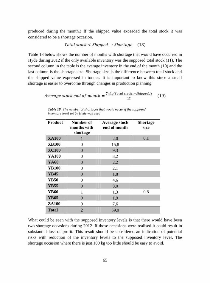
65

produced during the month.) If the shipped value exceeded the total stock it was

considered to be a shortage occasion.

Table 18 below shows the number of months with shortage that would have occurred in

Hyde during 2012 if the only available inventory was the supposed total stock (11). The

second column in the table is the average inventory in the end of the month (19) and the

last column is the shortage size. Shortage size is the difference between total stock and

the shipped value expressed in tonnes. It is important to know this since a small

shortage is easier to overcome through changes in production planning.

What could be seen with the supposed inventory levels is that there would have been

two shortage occasions during 2012. If those occasions were realised it could result in

substantial loss of profit. This result should be considered an indication of potential

risks with reduction of the inventory levels to the supposed inventory level. The

shortage occasion where there is just 100 kg too little should be easy to avoid.

Table 18: The number of shortages that would occur if the supposed

inventory level set by Hyde was used

Product Number of

months with

shortage

Average stock

end of month

Shortage

size

XA100 1 2,0 0,1

XB100 0 15,8

XC100 0 9,3

YA100 0 3,2

YA60 0 2,2

YB100 0 2,1

YB45 0 1,8

YB50 0 4,6

YB55 0 8,0

YB60 1 1,3 0,8

YB65 0 1,9

ZA100 0 7,6

Total 2 59,9

66

As the measure is in months with shortage, it could be interesting to see how many

orders were affected in those months. In January, when the shortage occasion for

XA100 happens there is just one order; hence it is just one order that cannot be fully

delivered. When there is a shortage for YB60 there are two orders which both are larger

than 800 kg. This means that one could be fully delivered, while the other one lacked

800 kg. Thus, in total two orders would have been affected during 2012. This gives an

order fill rate of 98,6%, which was found through the calculations in formula 20.

For XB100 and XC100, the average inventory level in the end of the month is very

high. As discussed earlier, the forecast for XC100 has a positive bias, which is a

probable cause to its high inventory level. For XB100 on the other hand, the reason is

probably the large safety stock Hyde AB has used, and in average 15,8 tonnes are left in

the finished goods inventory in the end of every month. The forecast for XB100 was

too small in 10 months 2012, but the safety stock was still sufficient.

67

Table 19 shows what the same result would look like with the safety stock developed in

the prior section.

With the developed safety stock there would have been only one shortage occasion

2012, and the average inventory level in the end of the month would go from 59,9

tonnes to 50,1 tonnes. In the month where the shortage occurred there were two orders

which both had a size larger than 400 kg, meaning that only one order would have been

affected. The order fill rate was found through the same calculations as above (18) and

gave the result 99,3%.

Previously in 5.1.2, the actual average inventory level during 2012 was compared to the

supposed average inventory level. If the developed safety stock would have been used

instead in those calculations, the cost saving from today would be 905 kSEK in

comparison to the 871 kSEK. The difference of 34 kSEK (905-871) is very small in the

context and there is not really any reason to use the developed safety stock instead of

the one Hyde uses today. The safety stock inventory levels are quite similar in size and

in number of shortage occasions. The developed one is slightly better in both cases, and

could give some inspiration for future safety stock dimensioning in Hyde.

Table 19: Number of shortage occasions and the average stock

in the end of the month with the developed safety stock

Product

variant

Number of

shortages

Average

stock end

of month

Shortage

size

XA100 0 2,1

XB100 0 10,4

XC100 1 8,8 0,4

YA100 0 3,9

YA60 0 1,6

YB100 0 2,2

YB45 0 2,2

YB50 0 3,8

YB55 0 2,9

YB60 0 2,3

YB65 0 2,0

ZA100 0 7,8

Total 1 50,1

68

5.2. POSTPONEMENT This section analyses how a postponement strategy would affect the tied up capital in

Hyde AB. The savings from postponement discussed here are the lower value of the

semi-finished goods and the delaying of product differentiation so that risk-pooling is

enabled. In the analysis the most suitable point of differentiation was firstly found for

every product. From these locations, the feasibility and profitability was investigated by

comparing the potential savings to the amount of extra production capacity needed. To

achieve a feasible solution, the production lead time had to be shorter than the

customers expected delivery time. Hyde shows many of the characteristics that make

postponement beneficial, as discussed in 3.5.2. The demand shows a lot of variability

and all products originate from the same SFG.

5.2.1. INTRODUCTION

In the finished goods inventory the lead time to customer is the shortest since all

products are already manufactured. If the correct inventory is stored a high service level

could be reached. To do this in a good way, very accurate forecasting is usually

necessary. Otherwise a very extensive safety stock might be needed in order to handle

the uncertainty of demand.

A way to solve this dilemma is to use a postponement strategy, where the benefits of

risk-pooling are taken advantage of. The production is then planned according to

forecasts until an intermediate storage at the point of differentiation, where the SFG

wait until a customer order arrives. If a postponement strategy would be used, a greater

flexibility in production capacity might be needed to match with fluctuating demand.

To analyse the postponement possibilities at Hyde AB, a simulation model of the

production was developed. The purpose was to understand how well the production

would be able to handle unplanned incoming orders. This is of importance when

finding the average and maximum production lead time for the investigated scenarios.

There is a trade-off between the production lead time and capacity; a greater capacity

increases the cost, but gives a higher throughput rate and better possibilities to decrease

the lead time to customer.

5.2.2. POSSIBLE INVENTORY LOCATIONS

In 3.5.1 different MTO and MTS alternatives were discussed. Figure 11 and 12 show

how a scenario could look like before and after postponement. In figure 11, the order

penetration point is in the “customised product inventory”, and the differentiation point

in the “generic component inventory”. Here the customer order arrives when the

product is already finished and there is no possibility of risk-pooling. In figure 12, a

69

Figure 11: Possible storage options

postponed scenario is shown. Here the OPP and DP are at the same location, and

products with the same generic SFG could be risk-pooled with each other.

There are, as mentioned in 4.2.2, three points of differentiation at Hyde AB; before

shaping, before oven and before mixing. Those are the postponement options and

together with the finished goods inventory the possible locations to place inventory.

After each differentiation point there is an increase in the number of product groups10

.

In figure 13, the different storage options are shown as well as the number of product

groups in each step. The earlier in the production process the inventory is held, the

more products share the generic SFG and the greater is the risk-pooling. The aim with

an implementation of postponement would be to move the OPP backwards. Thus, to go

from figure 11 which is the current situation to something more similar figure 12.

10

For example product group X becomes product groups XA, XB and XC.

Figure 12: The postponed situation Figure 11: The current situation

70

5.2.3. THE SIMULATION MODEL

The simulation model was developed with the purpose of finding the average and

maximum production lead time in different postponement scenarios when alternating

the capacity. The needed production capacity is vital as it directly affects the achieved

savings from postponement. Four plausible scenarios could be indentified and

simulated from studying possible risk-pooling opportunities at the points of

differentiation. How these four scenarios were found is shown further on in 5.2.5.-5.2.7.

To get a better understanding of the simulation model, it is described briefly further and

depicted in appendix 4. First the most important assumptions are clarified. These were

necessary in order to make the construction of the simulation model possible.

General Assumptions If a customer order included products that could go together in a specific machine they

were combined into a so-called matching group and produced together.

Each customer order was handed separately in the production process. It means that no

customer orders were combined into the same matching group, even though it may be

the case in reality. This made the simulated times slightly longer than they would be in

reality. One customer order could become one or more production orders depending on

the product.

With the tested scenarios the planning of the production would be somewhat different

than today. At the moment most volume is made-to-stock, and with the proposed

scenarios all or a great share would be made-to-order. To create a future situation with

both stochastically arriving customer orders (MTO) and MTS production orders being

produced at the same time, the priority function in ExtendSim was used. The customer

order history was generated into the model with a priority set on postponed MTO

products. This made prioritized products to go first into the system acting as a newly

arrived customer orders, while the SFG already in production caused delays to

prioritized orders, as in reality. In explicit, prioritised product groups were always

produced first but if there already were SFG in the machine the prioritised had to wait

until it was finished. The priorities depended on the scenario modelled.

The simulation model assumed that there were no shortages of material from supporting

machines not being part of the model. To achieve this supporting level in reality,

additional safety stock might have to be hold.

Mixing Machine In the mixing machine the matching groups were split into an integer number of load

carriers.

71

The mixing times were set specifically for each product group, XA, XB, YA etcetera.

Different product groups got different mixing times depending on their share of extra

material added since that is the driver of time. For example, YB has many large mixes

which takes longer time to produce. Because of that, its time in the mixing machine per

load carrier was longer than for the other product groups. To always produce filled load

carriers leads to some overproduction, in reality the production manager would have to

take this surplus into account when doing the detailed production planning.

Today, eight load carriers are usually filled in the mixing machine every time. In the

simulation model the machine was set to be more flexible and was loaded with one load

carrier at a time.

The time to walk to the mixing machine, change equipment and fill it was set to 30

minutes per load carrier.

Oven In the oven, the matching groups were split in the same way as in the mixing machine:

an integer number of load carriers were formed by dividing the matching group size by

the possible weight in a load carrier and rounding up. Since the batches were rounded

up some overproduction in the oven would result, in the same way as in the mixing

machine. In the long run, it would lead to slightly shorter production times than in the

simulation due to excessively produced inventory. If there are enough finished

products, nothing new would need to be produced. Since the quality of the end product

cannot be guaranteed if the load carriers are not filled, there is no option of not

overproducing.

When the number of ovens in reality is increased, it is likely that single ovens will be

replaced by double ovens to save space. In the simulation though, the incremental

adding of ovens was represented by single ovens. This means that the actual times in

the ovens would be slightly longer than the simulated times.

The last two simplifications have the opposite effect and aggregated they reduce the

error and give more accurate simulation times.

Shaping Due to the complexity of the shaping procedure it was not possible to model this part in

the same way as the other two steps, oven and mixing. Because of that the time in the

oven and mixing has been examined followed by an estimation of the extra time for the

shaping machine. This gave a useful approximation.

72

Description of the Model The simulation model can be found in appendix 4. To describe it briefly, all customer

orders during 2011 and 2012 were generated into the system. The model then splits the

customer orders into order lines and puts products with the same production

characteristics together in a matching group. These matching groups go firstly through

the oven and then pass by to the mixing machine. In both the oven and the mixing

machine the production orders are split into multiples of 625 kg to illustrate the SFG in

one load carrier. Depending on the scenario, the recorded time is either the completion

time of a matching group (scenario 1, 2, 3 described further) or completion time of an

order (scenario 4). The two different time measurements depend on if all products are

postponed or just a few.

5.2.4. CORRELATION COEFFICIENTS

When the correlation in demand between two products goes positive the benefit of risk-

pooling diminishes, and opposite. Two products with a high correlation will most often

be bought together; causing peaks and dips in demand to coincide, which in turn

reduces the risk-pooling. Because of that it was of interest to examine the correlation

between products that would be postponed together.

When doing this investigation, the customer order correlation had to be used instead of

the demand correlation. Customer order correlation looks at the correlation between

products on individual customer orders, instead of the total demand. This

approximation was necessary due to the large order sizes arriving within certain

intervals. Misleading correlation would otherwise appear between products if for

example two very large orders happen to coincide in the same month. Those orders are

not correlated with each other even though they arrive at the same time. When the

products are used by a customer however, there are certain combinations of products

that are sold more often. The dependency among these combinations appears if the

customer order correlation is used.

In table 20 the correlation coefficients exceeding 0,5 are presented. A complete table of

the correlation between all variants can be found in appendix 5. Correlation was

included in all future calculations in order to increase the accuracy of the results.

73

Table 20: Correlation coefficient based on demand

variability

Product variants Correlation

coefficient

YA70 YA55 0,9

YA60 YA100 0,6

YB50 XB100 0,6

YB50 YB65 0,5

Between most variants the correlation coefficient is close to zero. An interesting

observation though, is that high correlation is shown within the YA group. Between the

two MTS-products, YA100 and YA60, the correlation is 0,6 and between YA70 and

YA55 as large as 0,9. Due to the high correlations, the gain of postponing the order

penetration point for only YA becomes smaller. The products in the YA group are

standing for a very small share of the total demand (2,2 %) and the effort to postpone

this group is probably not profitable anyway.

YB50 and XB100 are the two variants that sell the most and the correlation of 0,6

would negatively affect the profitability if these products are postponed together. The

only point of differentiation they have in common though is before shaping.

During 2012 YB50 and YB65 were the two YB-products with the largest sales, and

their correlation of 0,5 can have impact on the gains from risk-pooling.

5.2.5. BEFORE MIXING

The points of differentiation are now examined more thoroughly, and the analysis starts

with the location before mixing. There is no intermediate storage before mixing today

except from load carriers waiting for the machine. The order penetration point and

finished goods inventory is today positioned just after this differentiation point.

Grouping of Products This section shows the reader possible risk-pooling opportunities between different

products just before mixing.

The mixing is the last point of differentiation and, as seen in figure 13, the six product

groups before mixing becomes 23 finished products afterwards. When comparing charts

16 and 17 it is possible to see that there are great opportunities to risk-pool product

group YB. The seven products (chart 17) are one group (chart 16) before mixing and

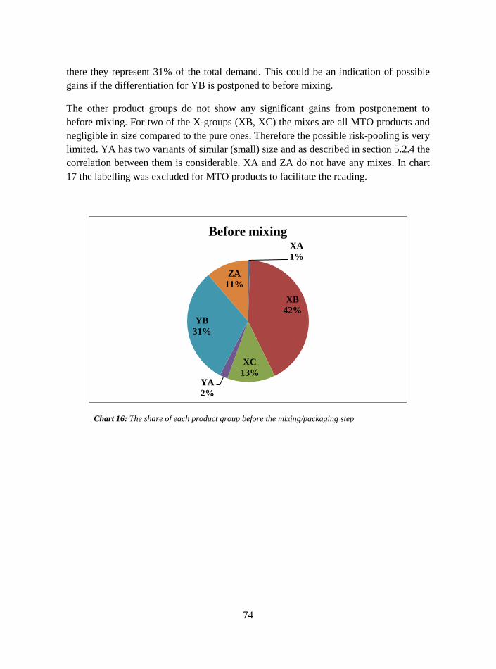
74

there they represent 31% of the total demand. This could be an indication of possible

gains if the differentiation for YB is postponed to before mixing.

The other product groups do not show any significant gains from postponement to

before mixing. For two of the X-groups (XB, XC) the mixes are all MTO products and

negligible in size compared to the pure ones. Therefore the possible risk-pooling is very

limited. YA has two variants of similar (small) size and as described in section 5.2.4 the

correlation between them is considerable. XA and ZA do not have any mixes. In chart

17 the labelling was excluded for MTO products to facilitate the reading.

Chart 16: The share of each product group before the mixing/packaging step

XA

1%

XB

42%

XC

13% YA

2%

YB

31%

ZA

11%

Before mixing

75

Chart 17: The share of sold volume for each product

According to the discussions above, the preferable option is to postpone group YB only,

since the other products would not contribute to any significant risk-pooling in this step.

Therefore postponing YB is the only scenario that is developed for this storage option.

To postpone too many products would result in unnecessarily high production

requirements.

Safety Stock Levels In this part the risk-pooling opportunities for product group YB is further specified.

First the possibilities for decreased demand variability are shown, followed by a

presentation of the new safety stock with corresponding savings from reduced tied up

capital.

In table 21, the standard deviation of demand during 2012 is shown for all YB products.

To calculate the risk-pooling, the aggregation formula in 3.5.2 has been used. The

formula uses the standard deviation to allocate the risk and find the aggregated

uncertainty. The correlation is also included. By doing this, it is found that the

aggregated standard deviation decreases with about 59 % if the YB products are

postponed to before mixing. The safety stock is a measure of the demand uncertainty

and as the risk is decreased 59 %, the new safety stock in postponement is assumed to

also decrease with 59 %.

XA100

1%

XB100

42%

XC100

13%

YA100

1%

YA60

1%

YB100

2%

YB45

2%

YB50

14%

YB55

2%

YB60

3%

YB65

7% YB70

2%

ZA100

11%

Finished goods inventory

76

In table 23 the enabled savings are shown, as a function of the new safety stock and the

one used today. This value is calculated in formula 21 and the inventory carrying

charge is also her set to be the internal rate of return.

Table 21: Standard deviations for all YB

products and the potential reduction if

postponed

Product Standard

deviation, 2012

YB100 1704

YB45 699

YB50 2219

YB55 643

YB60 1003

YB65 1314

YB70 764

Sum 8345

Postponement 3411

Reduced

variability 59%

Table 22: List of symbols

Symbols Explanation

safety stock new

safety stock today

i internal rate of return

vm value before mixing

vFGI

value in the finished goods

inventory

77

The possible savings from risk-pooling would be about 98 kSEK per year. The risk of

shortage with the new safety stock was analysed in the same way as in 5.1.2. No

shortage occasions appeared when using that method.

The value of the SFG at different points in the production was set to be dependent on

the value adding time. A thorough analysis of the value adding time was outside the

scope of this project, but the value of the finished products and the raw material per kg

was already known in the company. The approximated value of the SFG in different

storage locations was then dependent on the lead time from the previous location. The

SFG were assumed to have 60% of its final value before shaping, 70% before the oven

and 90% before the mixing.

Cycle Stock

A postponement solution does not only influence the safety stock but also the cycle

stock. If an intermediate storage is to be built earlier in the production process, the

value of the cycle stock held there is lower. This does affect the savings from a

postponement solution positively. As mentioned previously in Safety Stock Levels, the

semi-finished goods before mixing are said to have 90% of the total value of the

finished products. The average cycle stock is calculated from formula 12 minus the

safety stock. Thus, the semi-finished goods are assumed to be produced according to

forecasts as today, but without the overproduction of today.

The reduced cost of tied up capital due to lowered value is 17 kSEK per year and is

found through the calculation in (22). The average cycle stock per month during 2012 is

multiplied by the internal rate of return and the difference in value between the FGI and

the step where the product is stored.

Table 23: The potential cost reduction with postponement

Safety stock, today 13000 kg

Safety stock, new 5330 kg

Reduced cost of tied-up

capital 98 kSEK

78

Table 24: List of symbols

Symbols Explanation

SI

supposed average

inventory level

safety stock today

i internal rate of return

vm value before mixing

vFGI

value in the finished

goods inventory

The total reduced cost for both safety stock and cycle stock is thereby 115 kSEK per

year (98+17).

Production Concerns The lead time from “before mixing” to the finished goods inventory could be fairly

short but is dependent on the batch size and product group. For the interested reader

table 6 in section 4.2.2 presents the production rate for each product. These rates have

been used to find the product group specific times in the mixing machine. In the

simulation, YB was given first priority to illustrate the arrival of a customer order.

In chart 18, it is possible to see the maximum and average lead time for an order of YB-

products to pass through the mixing step. A conclusion that can be drawn from studying

the chart is the decreasing marginal benefit of additional mixing machines. To invest in

one mixing machine decreases the maximum time from 4,7 days to 2,4 and the average

lead time from 1,3 to 0,7, which is a halving of the production time. If yet another

mixing machine is purchased the marginal benefit decreases significantly as the

maximal time goes from 2,4 to 1,7 and the average time from 0,7 to 0,5. This is a time

reduction of about 30 %. To have four mixing machines is not very plausible in reality,

and if the times are compared, there is no significant decrease in the average time at all

from having three machines. These times are also shown in table 25 below.

79

The usual delivery time the customer can expect is shipment of the order from the

production facility after one week. Within this time one to two days are needed to pack

the order. When considering one mixing machine, a maximum value of 4,7 + 2 = 6,7

days should be acceptable. The average time is 3,3 days when preparation is included.

Potential Cost Savings The cost of an additional mixing machine must be compared to the savings from

reducing the tied up capital. To do this the method of net present value was used (10).

0,0

0,5

1,0

1,5

2,0

2,5

3,0

3,5

4,0

4,5

5,0

1 mixing

machine

2 mixing

machines

3 mixing

machines

4 mixing

machines

Nu

mb

er o

f d

ay

s

Max-/ average lead time

Average

Max

Table 25: Average and max lead times for YB

through the mixing/packaging step

Production

lead times

Average Max

1 mixing

machine 1,3 4,7

2 mixing

machines 0,7 2,4

3 mixing

machines 0,5 1,7

4 mixing

machines 0,5 1,3

Chart 18: Max and average lead time for YB products through the mixing/packaging step.

80

This calculation is dependent on the payback time period, internal rate of return and the

price of new machines. These are confidential numbers to Hyde AB, but to give a

feeling of the result the following example have been developed with fictive numbers.

Pay-back time: 7 years

Internal rate of return: 7%

Potential savings per year from reduced tied up capital: 115 000 SEK

Initial cost: Machine cost

Number of additional mixing machines: 1

IC = 620 000 SEK

Table 26: List of symbols

Symbols Explanation

n Payback time

i Internal rate of return

R Net cash flow

IC Initial cost

y Year 1, 2,...,n

From this expression, IC could be found as 620 kSEK, which means that this is the

maximum amount of money Hyde could invest in a new mixing machine. If the whole

amount is used the investment is indifferent to the profitability.

5.2.6. BEFORE OVEN

The second option investigated was to postpone to the location before the oven. Here

the differentiation occurs in the oven, and there is no intermediate storage at this

location today except from load carriers waiting for an idle oven.

81

X

56%

Y

33%

Z

11%

Before oven

Chart 20: The share of each product group before the oven

Grouping of Products Before the oven there are three different product groups: X, Y, and Z. As mentioned

earlier, Z remains the same throughout the process, hence there is no possibility to risk-

pool in the location before the oven. Charts 19 and 20 show the share of the volume for

every product group “before oven” and “before mixing”. When those two charts are

compared it is possible to draw some conclusions.

XA

1%

XB

42%

XC

13%

YA

2%

YB

31%

ZA

11%

Before mixing

Chart 19: The share of each product group before the mixing/packaging step

82

Firstly, there is a possibility for risk-pooling of X-products. There are three X-variants

before the oven representing 42%, 13%, and 1% of the total sold volume. Even though,

as discussed in section 3.5.2, postponement is more beneficial when products show

similar demand characteristics, it could be interesting to identify the possible gains in

this case.

For Y-products on the other hand, the risk-pooling is not as large, YB represents 31%

of the volume before mixing and, compared to that, YA is small with 2% of the total

volume. An inclusion of Y would result in small gains and a lot of extra production

capacity, since 33% of the products would be postponed.

The further investigation of the oven does only cover the postponement of X. Two

different scenarios were investigated, since it was also found in the prior part (5.2.5)

that postponing YB to before the mixing was beneficial. These two scenarios are; if just

X is postponed, and secondly if X is postponed before the oven and YB before mixing.

Safety Stock Levels The main gains from risk-pooling to before oven would be the postponement of product

group X. In this case, only the pure products had to be considered. All the mixes are

negligible; the demand is limited to up to a few hundred kilos per year. As shown in

table 27, the demand variability could be reduced by 37% when X is postponed to

before oven.

Table 27: Standard deviation for X

products and the potential reduction if

postponed

Product Standard

deviation

XA100 451

XB100 5368

XC100 3366

Sum 9185

Postponement 5748

Reduced

variability 37%

83

The new safety stock is given in table 28 below. These values are calculated in the same

way as explained in before mixing (5.2.5). What could be seen is that the saving in

percent (37%) is smaller than for postponing YB to before mixing, but that the reduced

cost of tied up capital is larger (189 kSEK). This is because the safety stock for XB100

is very large today and that the SFG value is considerably lower before oven than

before mixing. The risk of shortage with the new safety stock was analysed in the same

way as in 5.1.2. No shortage occasions appeared when using that method.

Cycle Stock

The lower value of the cycle stock would reduce the cost of tied up capital in the same

way as in the scenario before mixing. Formula 22 has been used to do the calculations,

with the difference that the value of the SFG before the oven is used instead of mixing

The reduced cost due to lowered value of the cycle stock is 40 kSEK. In total, the

annual reduction of cost for tied up capital from safety stock plus cycle stock would be

229 kSEK (189+40).

If both X and YB (before mixing) is postponed, the savings would be 229 kSEK plus

the 115 kSEK from YB. The total savings are then 344 kSEK.

Production Concerns The ovens are currently the bottleneck in the production, with a production rate of 76

kg/hour and a value-adding time of normally 41 or 42 hours. This scenario resulted

naturally in both a longer lead time and a greater production uncertainty than the option

“before mixing”, since in this scenario the SFG pass through both the oven and the

mixing. In contrary to the mixing machine, one batch in the oven can only create one

outcome. It is necessary to produce in full batches of 625 kg, which cause over-

production.

Postpone X to Before Oven

The oven and mixing machine was simulated together to give a hint of how much the

production capacity would need to increase in order to finish the production orders

Table 28: Possible cost reduction when postponing

Safety stock, today 28000 kg

Safety stock, new 17522 kg

Reduced cost of tied-up

capital 189 kSEK

84

within the delivery time. Table 29 shows the average and maximum lead time for

product group X, from before the oven until the finished goods inventory.

In this simulation only the results for product group X were studied, the other groups

were assumed to be produced to stock and the lead times of those were therefore of less

interest. The simulation showed that it is not possible to have just one mixing machine

as the production lead time reaches a maximum of between 10,2 and 11,9 days

depending on the amount of ovens. Even though these values are only attained a few

times every year, it could be troublesome for a customer focused company as Hyde.

To buy a new mixing machine shows good marginal benefits, as seen in chart 21 below.

At the same time, the benefit from three mixing machines was limited. This example is

of having six ovens, but the same pattern is also shown for other combinations. With

the production volumes of today, the optimal number of mixing machines would

therefore be two.

Table 29: The average and maximum lead times for product group X from

the oven to the finished goods inventory

1 mixing

machine

2 mixing

machines

3 mixing

machines

5 ovens Max 11,9 11,1 11,1

Average 5,2 4,6 4,5

6 ovens Max 11,5 9,3 8,6

Average 4,6 4,0 3,8

7 ovens Max 11,0 8,8 8,5

Average 4,3 3,7 3,5

8 ovens Max 10,2 8,6 7,9

Average 4,0 3,4 3,2

85

Chart 21: Marginal benefit of additional mixing machines, with six ovens

When it was decided that two mixing machines were the optimal, the most suitable

number of ovens had to be found. The marginal benefit between five and six ovens is

clearly noticeable in chart 22 below, but the numbers did not change significantly when

more ovens were added. When changing from six to eight ovens, the maximum time

changed from 9,3 days to 8,6 days. This indicated that the main cause of the long

delivery times is not the number of ovens, but the long production time in the ovens.

A problem is that the maximum times should not exceed one week including

preparation time of 1-2 days. It does not seem like a plausible solution to postpone

product group X to the location before oven. If Hyde changes the delivery time to a few

days longer, the proposed solution is six ovens and two mixing machines.

0

2

4

6

8

10

12

14

1 mix 2 mix 3 mix

Nu

mb

er o

f d

ay

s

Max & average lead time, six ovens

Max

Average

86

Table 30: Max and average lead times for X products if YB is postponed as well

1 mixing

machine

2 mixing

machines

3 mixing

machines

5 ovens Max 11,9 11,1 11,1

Average 5,3 4,6 4,5

6 ovens Max 11,5 9,3 8,6

Average 4,7 4,0 3,8

7 ovens Max 11,0 8,8 8,5

Average 4,7 3,7 3,5

8 ovens Max 10,3 8,6 7,9

Average 4,6 3,4 3,2

Chart 22: Marginal benefit of additional ovens, with two mixing machines

Postpone X before Oven and YB before Mixing

Another scenario considered was a combination of the two above; to store group X

before the oven and group YB before the mixing. All the other products were then

placed in the finished goods inventory. In table 30, it is possible to see that there was no

significant increase in lead times if YB was postponed as well. The only difference is

when there is one mixing machine, and it differs with only a couple of hours. Hence,

there is no reason to postpone just X. If both X and YB is postponed, the risk is slightly

increased, while the additional savings are much larger. However the investment cost

for the ovens should be compared to the gains from the postponement of group X only.

0,0

2,0

4,0

6,0

8,0

10,0

12,0

5 ovens 6 ovens 7 ovens 8 ovens

Nu

mb

er o

f d

ay

s

Max & average lead time, two mixing

machines

Max

Average

87

In chart 23 the marginal benefit from increasing the number of mixing machines is

shown, and in chart 24 the reduction in lead time when increasing the number of ovens

is depicted. Just as in the scenarios above the marginal benefit from a second mixing

machine is great but a third one does not reduce the lead times to any greater extent.

This scenario has the same lead time problems as discussed above for postponement of

only X. If postponement is made possible through longer delivery times, the

recommendation is two mixing machines and six ovens for this scenario as well.

Chart 23: Marginal benefit of additional mixing machines, with six ovens

Chart 24: Marginal benefit of additional ovens, with two mixing machines

0,0

2,0

4,0

6,0

8,0

10,0

12,0

14,0

1 mix 2 mix 3 mix

Nu

mb

er o

f d

ay

s

Max-/ average lead time, six ovens

Max

Average

0,0

2,0

4,0

6,0

8,0

10,0

12,0

5 ovens 6 ovens 7 ovens 8 ovens

Nu

mb

er o

f d

ay

s

Max-/ average lead time, two mixing

machines

Max

Average

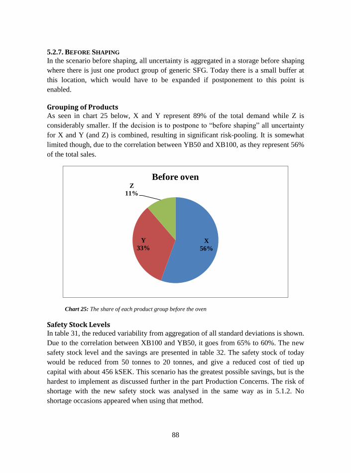
88

5.2.7. BEFORE SHAPING

In the scenario before shaping, all uncertainty is aggregated in a storage before shaping

where there is just one product group of generic SFG. Today there is a small buffer at

this location, which would have to be expanded if postponement to this point is

enabled.

Grouping of Products As seen in chart 25 below, X and Y represent 89% of the total demand while Z is

considerably smaller. If the decision is to postpone to “before shaping” all uncertainty

for X and Y (and Z) is combined, resulting in significant risk-pooling. It is somewhat

limited though, due to the correlation between YB50 and XB100, as they represent 56%

of the total sales.

Chart 25: The share of each product group before the oven

Safety Stock Levels In table 31, the reduced variability from aggregation of all standard deviations is shown.

Due to the correlation between XB100 and YB50, it goes from 65% to 60%. The new

safety stock level and the savings are presented in table 32. The safety stock of today

would be reduced from 50 tonnes to 20 tonnes, and give a reduced cost of tied up

capital with about 456 kSEK. This scenario has the greatest possible savings, but is the

hardest to implement as discussed further in the part Production Concerns. The risk of

shortage with the new safety stock was analysed in the same way as in 5.1.2. No

shortage occasions appeared when using that method.

X

56%

Y

33%

Z

11%

Before oven

89

Cycle Stock

Before the shaping, the SFG is said to have 60% of its final value. This step enhances

the greatest reduction in tied up capital for the cycle stock. With the same calculation as

in formula 22, the additional reduced cost for tied up capital due to the lower value of

the cycle stock is 157 kSEK. This results in a total cost reduction of 613 kSEK

(157+456).

Production Concerns Shaping is the first point of differentiation, thus to produce from here would incur the

longest lead times. This is because the products have to pass through every production

step in part B. In the other storage options some modifications can be done to only

include the most beneficial products. However, there is just one generic SFG before

mixing and the strength of this scenario is the inclusion of all products. This increases

the requirements on the production process. Another interesting aspect is that the

production time in part A is fairly short, which does not really encourage a storage

before shaping, but preferably before part A if a solution where all products would be

risk-pooled together was to be implemented. This is because the SFG has even less

value in the beginning of the process.

The safety stock volume would be 20 tonnes if all products were stored before shaping.

Today there is already a production buffer at this point with a maximum capacity of

10,75 tonnes. The storage would need to be increased with 186% to only meet the new

Table 31: Standard deviation for all products and

the potential reduction if postponed

Sum of standard deviations 23139

Sum of aggregated standard

deviations

9281

Reduced variability 60%

Table 32: Possible cost reduction when postponing

Safety stock, today 50000 kg

Safety stock, new 20054 kg

Reduced cost of tied-up

capital 456 kSEK

90

requirements of safety stock at this point. In addition to this, the forecasted demand

must be produced and stored in wait for orders.

Table 33 shows the average and maximum time for an order to pass through the

production process, without the inclusion of the shaping machine. By investigating the

lead time to produce all products from oven to the finished goods inventory, it is

possible to discard this option. Even with large investments (to a point where there are

eight ovens, compared with today’s five and three mixing machines), the maximum

production lead time would not fall below 9,6 days which is too much to guarantee

timely deliveries. The lowest average is 4,1 days, which is also too high as neither the

maximum nor the average include one to two days preparation for shipping or the time

in the shaping and granulation. The shaping would take at least an additional 12 hours,

and more during routine maintenance work. Today when all machines are maintained at

the same time there is a three days delay every 300 hours. That could be improved with

some re-scheduling, but probably not enough to save this option.

Just as in the prior scenarios, there is a very limited marginal benefit to have three

mixing machines compared to two. The trend is possible to see in chart 26. Chart 27 is a

depiction of the marginal benefit from additional ovens when there are two mixing

machines. The benefit diminishes quickly and is very small after the addition of a

seventh oven.

Table 33: Max and average order completion time for all products.

1 mixing

machine

2 mixing

machines

3 mixing

machines

5 ovens Max 26,5 25,8 25,8

Average 10,7 10,0 9,8

6 ovens Max 17,3 15,5 15,5

Average 7,5 6,5 6,3

7 ovens Max 14,2 11,8 11,8

Average 6,5 5,0 4,8

8 ovens Max 13,8 9,9 9,6

Average 6,1 4,4 4,1

91

0,0

5,0

10,0

15,0

20,0

1 mixing

machine

2 mixing

machines

3 mixing

machines

Nu

mb

er o

f d

ay

s

Max-/ average order completion time, six

ovens

Max

Average

Chart 26: Marginal benefit of additional mixing machines, with six ovens

Chart 27: Marginal benefit of additional ovens, with two mixing machines

0,0

5,0

10,0

15,0

20,0

25,0

30,0

5 ovens 6 ovens 7 ovens 8 ovens

Nu

mb

er

of

day

s

Max-/ average order completion time, two

mixing machines

Max

Average

92

5.2.8. HYBRID STRUCTURE

One possible option is to postpone only the uncertain demand. This could mean that the

average demand subtracted by for example one standard deviation is put in the FGI.

This would ease the pressure on the production when an order arrives and smoothen out

the needed capacity. This is not considered a safety stock, but as a part of the forecasted

demand. To store some demand in the FGI would slightly increase the tied up capital,

as the value of the products is greater than for the SFG.

In table 34 below it could be seen that three very popular variants would have their safe

demand in the finished goods inventory with this method. XB100 would have the most

with eight tonnes.

Table 34: Possible hybrid solution

Average demand 2011 One standard deviation To store in

FGI

XA100 263 551 0

XB100 14001 5784 8000

XC100 6052 3921 2000

YA100 2173 2518 0

YA60 525 637 0

YB100 646 1836 0

YB45 220 400 0

YB50 3713 1858 2000

YB55 1682 1489 0

YB60 769 1020 0

YB65 1244 848 0

YB70 17 0 0

ZA100 3721 3365 0

12000

93

6. CONCLUSION

This chapter summarises the findings in the analysis and discuss how those answer to

the purpose and research question asked in the introduction. The first part in the

analysis was a thorough review of the inventory levels. This was followed by an equally

thorough investigation of the possibilities and implications of implementing a

postponement strategy. This chapter presents the conclusions in this order and

eventually shows the recommendations.

6.1. INVENTORY LEVELS This part first shows the main findings from the investigation of the inventory levels,

followed by possible reasons to the situation today and potential savings if it is

changed. Important to notice though is that this analysis was not only important on its

own, but also for the understanding of the savings from postponement. If the

inventories are wrongly dimensioned, the generated potential savings from

postponement could appear wrong.

6.1.1. MAIN FINDING

In the Inventory Management part (5.1) of the analysis the main finding was a

confirmation of the perceived high inventory levels in the finished goods inventory. The

total inventory level was close to twice as large as the supposed level set by Hyde

themselves (safety stock + forecast), resulting in excessive tied up capital. For YB55

the inventory level was about 3,75 times larger than supposed. Important to notice is

that the forecasts were fairly accurate and that the safety stock levels were good for

most products. A review was also carried out to look upon if the supposed inventory

levels would have been sufficient to avoid stock outs in 2012. It showed two stock-out

occasions during the year, where, if the supposed levels were followed, there could

have been delivery problems.

6.1.2. POSSIBLE REASONS

The authors have limited knowledge and experience about the company but have

identified two possible reasons to this situation. First and foremost, today the

production is quite inflexible; the mixing machine is always fed with eight load carriers

(5000 kg). This is done even though the setup-time is limited compared to the total

production time. According to the economy of scale (3.3.1) it is favourable to produce

in large batches to enable allocation of the setup-time between many pieces (thus

94

reduce the cost per piece). If the setup-time is short, the powerfulness of economies of

scale is limited. Instead the benefits from flexible production could be stronger.

Ritzman and King (3.2.5) found that producing in correct batch sizes has larger

influence on reaching the correct inventory levels than both low forecast bias and good

forecast accuracy.

Another reason to the high inventory levels is that the production produces as much as

possible at all times, which results in more finished products than demanded. The

background to this is planned partial standstills due to a capacity expansion the

upcoming years. To cater for the demand during that period, the inventories have been

pushed up. The exceeding inventory levels (the inventory that is not forecasted, excess

from last month or safety stock) are enough to cater for the total demand during almost

four months, which appear to be more than necessary for this expansion. However, the

expansion project cannot fully explain the high inventory levels during the beginning of

2011, which most products show.

6.1.3. POTENTIAL SAVINGS

The potential savings were found to be 871 kSEK per year if the actual inventory levels

followed the supposed levels. These levels would have resulted in two delayed orders

2012, which could have been very expensive, especially if the reputation is impaired or

the customer changes to a competitor. One of these orders had a shortage of only 100

kg, and could probably be fulfilled with flexible planning. The other shortage would

have been about 800 kg and could have caused greater problems, since the amount

equals two load carriers.

In the project, a redistributed safety stock that is slightly smaller than the current was

developed from a method considering especially the maximum forecast error and the

bias. With this method, data from 2011 was used to create a new safety stock for 2012,

which was then tested and gave one shortage occasion. The potential annual savings

with the new safety stock compared to the one developed by Hyde is 34 kSEK per year.

Since the additional saving is rather small and some extra work would be required,

there is no reason for Hyde to change their safety stock dimensioning method from the

one used today. Never the less, the method can instead give some inspiration to the

future creation of safety stocks in Hyde.

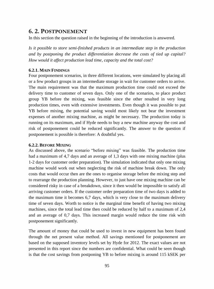
95

6. 2. POSTPONEMENT In this section the question raised in the beginning of the introduction is answered.

Is it possible to store semi-finished products in an intermediate step in the production

and by postponing the product differentiation decrease the costs of tied up capital?

How would it affect production lead time, capacity and the total cost?

6.2.1. MAIN FINDINGS

Four postponement scenarios, in three different locations, were simulated by placing all

or a few product groups in an intermediate storage in wait for customer orders to arrive.

The main requirement was that the maximum production time could not exceed the

delivery time to customer of seven days. Only one of the scenarios, to place product

group YB before the mixing, was feasible since the other resulted in very long

production times, even with extensive investments. Even though it was possible to put

YB before mixing, the potential saving would most likely not bear the investment

expenses of another mixing machine, as might be necessary. The production today is

running on its maximum, and if Hyde needs to buy a new machine anyway the cost and

risk of postponement could be reduced significantly. The answer to the question if

postponement is possible is therefore: A doubtful yes.

6.2.2. BEFORE MIXING

As discussed above, the scenario “before mixing” was feasible. The production time

had a maximum of 4,7 days and an average of 1,3 days with one mixing machine (plus

1-2 days for customer order preparation). The simulation indicated that only one mixing

machine would work out when neglecting the risk of machine break down. The only

costs that would occur then are the ones to organise storage before the mixing step and

to rearrange the production planning. However, to just have one mixing machine can be

considered risky in case of a breakdown, since it then would be impossible to satisfy all

arriving customer orders. If the customer order preparation time of two days is added to

the maximum time it becomes 6,7 days, which is very close to the maximum delivery

time of seven days. Worth to notice is the marginal time benefit of having two mixing

machines, since the total lead time then could be reduced by half to a maximum of 2,4

and an average of 0,7 days. This increased margin would reduce the time risk with

postponement significantly.

The amount of money that could be used to invest in new equipment has been found

through the net present value method. All savings mentioned for postponement are

based on the supposed inventory levels set by Hyde for 2012. The exact values are not

presented in this report since the numbers are confidential. What could be seen though

is that the cost savings from postponing YB to before mixing is around 115 kSEK per

96

year. In the example on page 80, the internal rate of return is 7% and the pay-back time

seven years. With these numbers, 620 kSEK (lower with true values) could maximally

be spent on buying a new mixing machine. This money would probably not be enough

to cover the purchase of another machine. The production is today in the middle of an

expansion project and if one more machine is to be bought anyway, the solution of

postponing YB to before mixing could become profitable with a lower risk.

The “before mixing” scenario is also supported by Swaminathan & Lee (section 3.5.7).

They found that late postponement is the most beneficial option if the production lead

time for the middle step is much longer than the lead times for the steps before and

after. In this case the oven takes much longer time than both the mixing and the

shaping. This could be seen as an indicator of where to put the storage even though the

demand does not fulfill the requirements of for example normal distribution.

A benefit of the “before mixing” scenario compared to the others is also the lower risk.

Earlier in this section the risk of having only one mixing machine was mentioned, but

in comparison with the other scenarios the total risk is smaller. Reduced risk originates

mainly from two factors. Firstly, the mixing is the last part of the production, thus the

risk of standstill comprises only one step. If one of the other scenarios would be chosen,

the risks are found in all the remaining production steps. Secondly, the production is

more flexible in the mixing than the other steps. If necessary, the amount produced can

be exactly what is needed while in the oven it has to be batches of 625 kg.

To reduce the requirements on the production even more, it is advisable to make use of

the hybrid solution discussed in the end of the analysis and produce a part of the

demand straight to FGI.

6.2.3. BEFORE OVEN

For the before oven solution two different scenarios were investigated; one where only

product group X was postponed and one where X was postponed to before the oven and

YB to before mixing. The scenarios showed almost identical characteristics regarding

production lead time but naturally, if YB was postponed as well, the potential savings

were greater. Hence, to only postpone X does not make any sense. The total potential

saving for X and YB combined, without including the cost for increased capacity, is

344 kSEK per year.

As mentioned in 6.2.1 this scenario is not feasible. Even with eight ovens and three

mixing machines the maximal production time is almost eight days. A more plausible

solution with six ovens and two mixing machines would result in a maximum lead time

97

close to nine days and an average of four days (plus customer order preparation time of

1-2 days).

The oven is the bottleneck of the production, in explicit the step with the lowest

production rate. As discussed in 3.6.1, a bottleneck has to be used in an optimal way

since it is the main inducer on the total production rate. Not only is the oven the

bottleneck, the production time is also long, one load carrier spends 41 hours in there.

In addition, the production in the oven has to be in full load carriers why the flexibility

is reduced. The low production rate, the long production time and the inflexible

characteristics of the step are also reasons to not postpone to before oven.

The only possibility to establish the storage before the oven would be to increase the

delivery time to customer with a few days. If eleven days could be accepted in

exceptional cases this solution would all of a sudden be possible. The average time

around six days is below today’s limit of seven. Those numbers are valid for six ovens

and two mixing machines, and include the order preparation time.

6.2.4. BEFORE SHAPING

The first point of differentiation is the shaping. Postponement in this step would be

beneficial of two reasons; the added SFG value is little and the risk-pooling is maximal

since there is just one generic product at this point. The possible gains from the scenario

were found to be 613 kSEK per year. Even though the savings are large, the production

lead time is too long even with major investments in production capacity.

To make this scenario possible the delivery time would need to increase to more than

two weeks and still two new ovens and one additional mixing machine would need to

be procured.

6.3. RECOMMENDATIONS The greatest potential savings and the lowest risk can be found if the size of the

inventory levels is reduced. Thus, that would be the natural place to start. It is also

necessary to have a good overview of what the inventory levels should be before

postponement can be realised, as it affects the size of the new storage location.

The first step to take is to allow more flexible production in the mixing machine. This is

necessary both to reduce the inventory levels and to enable postponement of YB. This

would not incur any extensive costs; the production staff will have to visit the location

more often but that can hopefully be managed if considered when scheduling.

98

An easy measure to reduce the risk of stock out is to have a more flexible production

planning. Today the production planning is updated every 20th day and with the current

inventory levels there is no reason to change. However, if the levels are decreased as

proposed, it could be advantageous to compare the forecasts and the incoming orders

more frequently. If a certain product is ordered more often or in greater volumes than

forecasted, this can be noticed early and the product would be given a higher priority.

This should act as a way to reduce the risk of having a shortage occasion.

The postponement of YB is seen as considerably risky with just one mixing machine.

At the same time, the savings are not large enough to pay for a new machine. Therefore

the postponement of YB is only recommended if a second mixing machine is procured

for other reasons.

The purpose of this report was to reduce the tied up capital for Hyde with the strategies

of inventory reduction and postponement. Further, clear recommendations about how to

implement the findings was also supposed to be given. In the thorough review of the

inventory levels, possible savings were indicated. How to implement the findings is

clearly summarised above. To sum up, the purpose of the report has been fulfilled.

6.4. ADDITIONAL OBSERVATIONS The forecasts were reviewed and were found to be relatively good. The standard

deviations of the forecast errors (forecast accuracy) are however in general quite large

which indicates the difficulties with forecasting the correct month of order arrival.

Today there is already some collaboration with the customers to find the reason to why

orders do not arrive when planned. If this collaboration could be extended further, it

would give an opportunity to even better forecasts. If the forecasting improves, there

would also appear possibilities to reduce the safety stock levels. Furthermore, the

average cycle stock would most likely decrease due to less excess inbound inventory.

Today, the information systems at Hyde are rather outdated and it is hard to obtain

sufficient data to do accurate analysis. A system that gathers for example forecasts,

inventory levels and sales data would facilitate the creation of forecasts and safety

stocks in the future. Furthermore, it was hard to obtain product specific production data

from a longer period of time, as the production lead times are not logged in a detailed

way. This information could preferably also be identified and stored in a more efficient

way than today, to enhance future production analysis.

Currently a lack of load carriers has been a challenge in the production. A flexible

production in the mixing step would reduce this problem. At the moment a lot of load

99

carriers wait for eight of the same product group to be finished in the oven, and while

waiting they occupy a load carrier. If only the amount of load carriers that were

demanded got mixed at once, the waiting time and the number of occupied load carriers

would be reduced.

6.5. CRITICISM Even though this project has been performed at the authors’ best ability, there are

reasons to criticise it on a few points. The number of assumptions has been held to a

minimum. However, some have been necessary to be able to execute this project. One

of these was that the mean of the actual inventory level in the beginning of each month,

over the year, was representative for the average inventory level. To answer if this

simplification is justified is hard without having information about the true values, but

if the inventories are to be reduced according to the recommendation, the levels should

be followed more in depth during a few months of time. How the expansion project has

affected the overall inventory levels is also hard to know, and does probably also affect

the outcome of expected savings.

The production times used in the simulation model are not as reliable as wished for, as

there was no availability of data over an extended period of time. This resulted in a less

accurate simulation model which has to be taken into consideration while evaluating the

results in the project.

The value of the SFG was in this report estimated from knowing the initial value of the

raw material and the final value of the products. The production time in each machine

was then assumed to be the determining factor of value add-on. This estimation is

probably not 100% correct and could affect the presented savings from postponement.

If the company decides to further investigate the postponement results, the value of the

SFG could easily be changed and elaborated with.

Due to the inconvenience of data collecting, the developed safety stock method has

only been tested on 2012 with data from 2011. Preferably at least one more year should

have been tested to ensure the validity and reliability of the method. As all numbers

regarding the forecasts, inventory levels and shipping had to be rewritten into Excel

manually, it was regarded too time consuming to include one more year. This decision

was taken from the knowledge that the dimensioned safety stock did not differ

dramatically from the safety stock developed by Hyde themselves.

100

101

7. REFERENCES

Andersen, I., 1998. Den uppenbara verkligheten - Val av samhällsvetenskaplig metod.

1:14 red. Lund: Studentlitteratur .

Answers, n.d. Answers. [Online]

Available at: http://www.answers.com/topic/normal-distribution

[Accessed 04 02 2013].

Averkamp, H., n.d. Accounting coach - What is setup cost?. [Online]

Available at: http://blog.accountingcoach.com/what-is-setup-cost/

[Accessed 21 02 2013].

Axsäter, S., 2006. Inventory Control E-book. 2 red. Boston: Springer Science.

Blom, G. et al., 2005. Sannolikhetsteori och Statistikteori med tillämpningar. 5 ed.

Lund: Studentlitteratur.

Chopra, S. & Meindl, P., 2010. Supply Chain Management: Strategy, planning and

operation. 4 ed. New Jersey: Pearson Education.

Gibson, B. J. & Novack, R. A., 2008. Supply Chain managment: a logistics perspective.

8th ed. Mason: Cengage Learning.

Gold, R. L., 1958. Roles in Sociological Field Investigation. Social Forces, 36(1-4), pp.

217-223.

Graman, G. A. & Magazine, M. J., 2006. Implementation issues influencing the

decision to adopt postponement. International Journal of Operations & Production

Management,, 26(10), pp. 1068-1083.

Hartman, D., n.d. Chron. [Online]

Available at: http://smallbusiness.chron.com/cycle-stock-inventory-25218.html

[Accessed 24 04 2013].

Heakal, R., 2009. Investopia.com. [Online]

Available at: http://www.investopedia.com/articles/03/012703.asp#axzz2IJxHhbRq

[Accessed 18 01 2013].

102

Holme, I. M. & Solvang, B. K., 1997. Forskningsmetodik - om kvaliatativa och

kvantiativa metoder. 2:nd edition red. Lund: Studentlitteratur.

Höst, M., Regnell, B. & Runesson, P., 2006. Att genomföra examensarbete. Lund:

Studentlitteratur.

Jan, I., n.d. Accounting Explained. [Online]

Available at: http://accountingexplained.com/managerial/capital-budgeting/npv

[Accessed 19 04 2013].

Mattson, S.-A. & Jonsson, P., 2003. Produktionslogistik. Lund: Studentlitteratur.

Mattsson, S.-A., 2003. Normalfördelning och Poissonfördelning för bestämning av

säkerhetslager, Lund: Lund University.

McBride, D., 2003. EMS consulting group - The 7 Manufacturing Wastes. [Online]

Available at: http://www.emsstrategies.com/dm090203article2.html

[Accessed 18 02 2013].

New Mexico Department of Health, 2012. Indicator-Based Information System for

Public Health, "Reliability and Validity". [Online]

Available at: http://ibis.health.state.nm.us/resources/ReliabilityValidity.html

[Använd 14 02 2013].

Nilsson, A., 2006. Essays on Joint Replenishment and Multi-Echelon Inventory Systems

Licentiate thesis. Luleå: Luleå University of Technology.

Nilsson, B. I., 2013. Att starta processen… Att problematisera verkligheten är det

första steget mot ökad kunskap/insikt och kan inte hoppas över. Lund: Lund University.

Nyce, C., 2007. The Institutes. [Online]

Available at: http://www.aicpcu.org/doc/predictivemodelingwhitepaper.pdf

[Accessed 32 01 2013].

Oskarsson, B., Aronsson, H. & Ekdahl, B., 2006. Modern logistik - för ökad lönsamhet.

3 ed. Ljublanja: Liber.

Rafiei, H. & Rabbani, M., 2011. Order partitioning and Order Penetration Point

location in hybrid. Computers and Industrial Engineering, Volume 61, pp. 550-560.

103

Rahman, S.-u., 1998. Theory of constraints: A review of the philosophy and its

applications. International Journal of Operations & Production Management, 18(4),

pp. 336-355.

Ritzman, L. P. & King, B. E., 1993. The relative significance of forecast errors in

multistage manufacturing. Journal of Operations Management, Volym 11, pp. 51-65.

Rutner, S. M. & C. John Langley, J., 2000. Logistics Value: Definition, Process and

Measurement",. The International Journal of Logistics Management, 11(2), pp. 73-82.

Shan, H., u.d. National Program on Technology Enhanced Learning. [Online]

Available at: http://www.nptel.iitm.ac.in/courses/Webcourse-contents/IIT-

ROORKEE/INDUSTRIAL-ENGINERRING/part3/inventory/lecture1.htm

[Använd 04 05 2013].

Stillwater, R., 2003. Virginia Tech. [Online]

Available at:

http://www.sv.vt.edu/classes/ESM4714/Student_Proj/class03/stillwater/prj/

[Accessed 14 05 2013].

Strategos, n.d. Strategos - Consultants, Enineers, Strategists. [Online]

Available at: http://www.strategosinc.com/inventory.htm

[Accessed 22 01 2013].

Sullivan, T., 1998. Implementing the Theory of Constraints (TOC) In Production.

[Online]

Available at: http://www.ciras.iastate.edu/publications/CIRASNews/winter98/toc.htm

[Använd 18 02 2013].

Svennevig, J., n.d. Handelshöjskolen. [Online]

Available at:

http://home.bi.no/a0210593/Abduction%20as%20a%20methodological%20.pdf

[Accessed 14 05 2013].

Swaminathan, J. M. & Lee, H. L., 2003. Design for postponement. In: A. G. de Kok &

S. C. Graves, eds. Handbook of OR/MS on Supply Chain Management. Amsterdam:

North Holland Publishing Co.

The Economist, 2008. The Economist - Economies of Scale and Scope. [Online]

Available at: http://www.economist.com/node/12446567

[Accessed 14 02 2013].

104

Thomopoulos, N. T., 2005. Safety Stock and Forecast Error, Vancouver: Illinois

Institute of Technology.

Wallén, G., 1996. Vetenskapsteori och forskningsmetodik. 2:nd edition ed. Malmö:

Studentlitteratur.

WebFinance Inc., n.d. BusinessDictionary.com. [Online]

Available at: http://www.businessdictionary.com/definition/stock-keeping-unit-

SKU.html

[Accessed 18 01 2013].

Wong, H., Wikner, J. & Naim, M., 2009. Analysis of form postponement based on

optimal positioning of differentiation point and stocking decisions. International

Journal of Production Research, 47(5), pp. 1201-1224.

Young, B., Burns, N. D. & Backhouse, C. J., 2004. Management of uncertainty through

postponement. International Journal of Production Research, 42(6), pp. 1049-1064.

Interviews:

18 December 2012, Financial Manager, Production Manager, Product Manager and

Customer Relationship Manager

5 February 2013, Financial Manager, Production Manager, Product Manager,

Production Planner, Production Operators (2)

In addition to this, frequent mail conversations with the ones mentioned above and the

Operations Engineer

i

8. APPENDIX

8.1. APPENDIX 1: SHIPPED AND FORECASTED

0

500

1000

1500

2000

2500

kg

of

pro

du

ct

Shipped & Forecasted XA100

Forecasted

Shipped

0

5000

10000

15000

20000

25000

kg

of

pro

du

cts

Shipped & Forecasted XC100

Forecasted

Shipped

ii

0

1000

2000

3000

4000

5000

6000

7000

8000 k

g o

f p

rod

uct

Shipped & Forecasted YA100

Forecasted

Shipped

0

1000

2000

3000

4000

5000

6000

7000

kg

of

pro

du

ct

Shipped & Forecasted YB100

Forecasted

Shipped

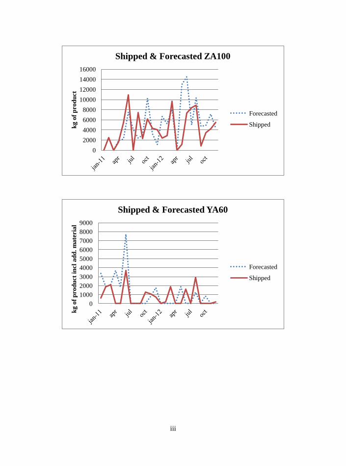
iii

0

2000

4000

6000

8000

10000

12000

14000

16000 k

g o

f p

rod

uct

Shipped & Forecasted ZA100

Forecasted

Shipped

0

1000

2000

3000

4000

5000

6000

7000

8000

9000

kg

of

pro

du

ct i

ncl

ad

d.

ma

teria

l

Shipped & Forecasted YA60

Forecasted

Shipped

iv

0

1000

2000

3000

4000

5000

6000

7000

8000

9000 k

g o

f p

rod

uct

in

cl a

dd

. m

ate

ria

l

Shipped & ForecastedYB45

Forecasted

Shipped

0

2000

4000

6000

8000

10000

12000

kg

of

pro

du

ct i

ncl

ad

d.

ma

teria

l

Shipped & Forecasted YB55

Forecasted

Shipped

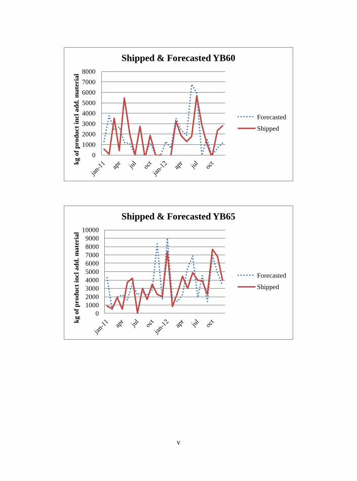
v

0

1000

2000

3000

4000

5000

6000

7000

8000 k

g o

f p

rod

uct

in

cl a

dd

. m

ate

ria

l

Shipped & Forecasted YB60

Forecasted

Shipped

0

1000

2000

3000

4000

5000

6000

7000

8000

9000

10000

kg

of

pro

du

ct i

ncl

ad

d.

ma

teria

l

Shipped & Forecasted YB65

Forecasted

Shipped

vi

0

500

1000

1500

2000

2500

3000

3500

jan-1

2

feb

mar

apr

may

jun

jul

aug

sep

oct

no

v

dec

kg

of

pro

du

ct i

ncl

ad

d.

ma

teria

l

Shipped & Forecasted YB70

Forecasted

Shipped

vii

8.2. APPENDIX 2: INVENTORY LEVELS

0

5000

10000

15000

20000

25000

30000

35000

40000

kg

of

pro

du

ct

XC100 Inventory level

Actual

Safety stock

Target

0

500

1000

1500

2000

2500

3000

3500

4000

4500

kg

of

pro

du

ct

XA100 Inventory level

Actual

Safety stock

Target

viii

0

5000

10000

15000

20000

25000 k

g o

f p

rod

uct

YA100 Inventory level

Actual

Safety stock

Target

0

2000

4000

6000

8000

10000

12000

14000

kg

of

pro

du

ct

YB100 Inventory level

Actual

Safety stock

Target

ix

0

5000

10000

15000

20000

25000 k

g o

f p

rod

uct

ZA100 Inventory level

Actual

Safety stock

Target

0

1000

2000

3000

4000

5000

6000

7000

8000

9000

kg

of

pro

du

ct

YA60 Inventory level

Actual

Safety stock

Target

x

0

1000

2000

3000

4000

5000

6000

7000

8000

9000 k

g o

f p

rod

uct

YB45 Inventory level

Actual

Safety stock

Target

0

2000

4000

6000

8000

10000

12000

14000

16000

18000

kg

of

pro

du

ct

YB50 Inventory level

Actual

Safety stock

Target

xi

0

2000

4000

6000

8000

10000

12000

14000 k

g o

f p

rod

uct

YB55 Inventory level

Actual

Safety stock

Target

0

1000

2000

3000

4000

5000

6000

7000

8000

9000

kg

of

pro

du

ct

YB60 Inventory level

Actual

Safety stock

Target

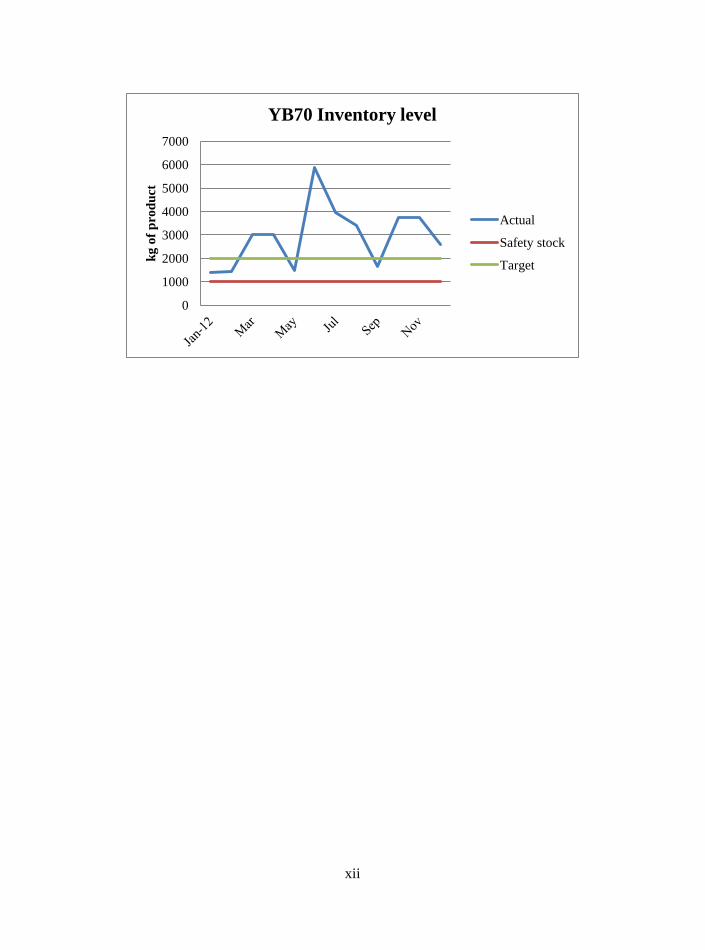
xii

0

1000

2000

3000

4000

5000

6000

7000 k

g o

f p

rod

uct

YB70 Inventory level

Actual

Safety stock

Target

xiii

8.3. APPENDIX 3: SHIPPED & INVENTORY

0

500

1000

1500

2000

2500

3000

3500

4000

4500

kg

of

pro

du

ct

Shipped & Actual inventory level XA100

Shipped

Actual

0

5000

10000

15000

20000

25000

30000

35000

40000

kg

of

pro

du

ct

Shipped & Actual inventory level XC100

Shipped

Actual

xiv

0

5000

10000

15000

20000

25000 k

g o

f p

rod

uct

Shipped & Actual inventory level YA100

Shipped

Acual

0

2000

4000

6000

8000

10000

12000

14000

kg

of

pro

du

ct

Shipped & Actual inventory level YB100

Shipped

Actual

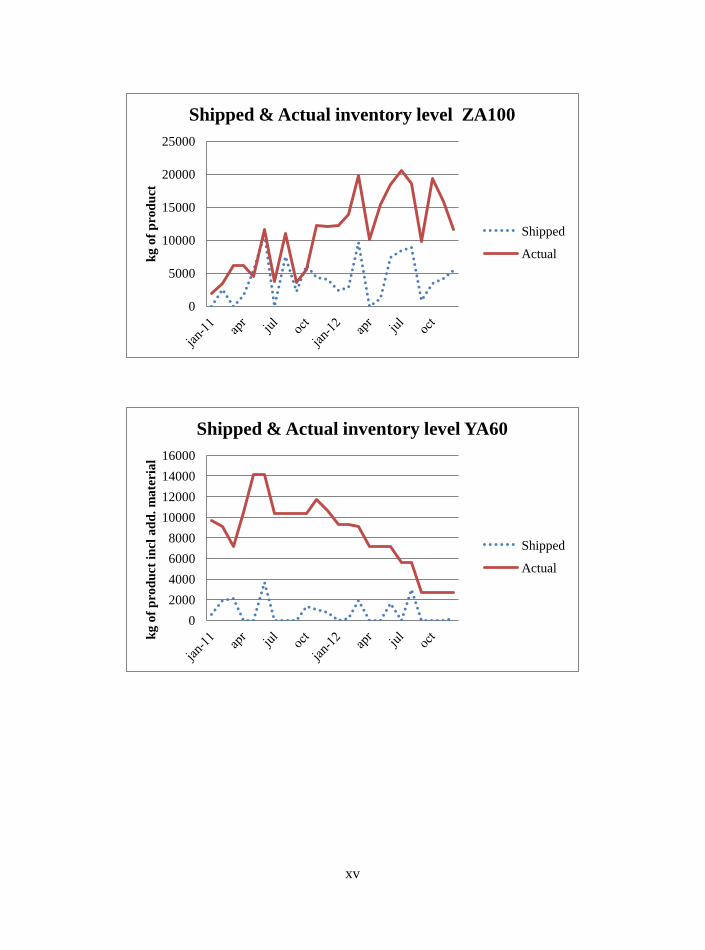
xv

0

5000

10000

15000

20000

25000 k

g o

f p

rod

uct

Shipped & Actual inventory level ZA100

Shipped

Actual

0

2000

4000

6000

8000

10000

12000

14000

16000

kg

of

pro

du

ct i

ncl

ad

d.

ma

teria

l

Shipped & Actual inventory level YA60

Shipped

Actual

xvi

0

5000

10000

15000

20000

25000 k

g o

f p

rod

uct

in

cl a

dd

. m

ate

ria

l

Shipped & Actual inventory level YB45

Shipped

Actual

0

5000

10000

15000

20000

25000

30000

35000

40000

kg

of

pro

du

ct i

ncl

ad

d.

ma

teria

l

Shipped & Actual inventory level YB50

Shipped

Actual

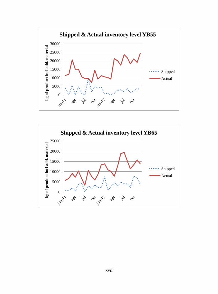
xvii

0

5000

10000

15000

20000

25000

30000 k

g o

f p

rod

uct

in

cl a

dd

. m

ate

ria

l

Shipped & Actual inventory level YB55

Shipped

Actual

0

5000

10000

15000

20000

25000

kg

of

pro

du

ct i

ncl

ad

d.

ma

teria

l

Shipped & Actual inventory level YB65

Shipped

Actual

xviii

0

1000

2000

3000

4000

5000

6000

7000

8000

9000

10000 k

g o

f p

rod

uct

in

cl a

dd

. m

ate

ria

l

Shipped & Actual inventory level YB70

Shipped

Actual

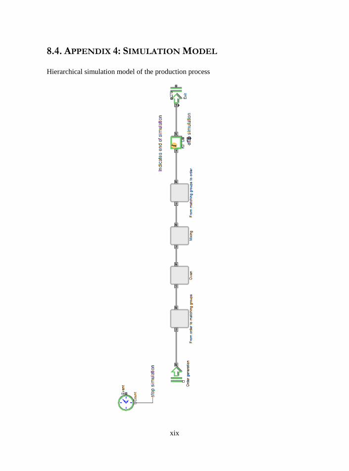
xix

8.4. APPENDIX 4: SIMULATION MODEL

Hierarchical simulation model of the production process

xx

From order to matching groups

xxi

Oven

xxii

Mixing

xxiii

From matching groups to order

xxiv

8.5. APPENDIX 5: CORRELATION COEFFICIENTS

XA100 XB100 XC100 YA100 YB100 ZA100 XB55 XB60 XB70 XC50 XC60 XC70 YA50 YA55 YA60 YA70 YB45 YB50 YB55 YB60 YB65 YB70

XA100 1,0 0,3 -0,1 0,0 0,0 0,0 0,0 0,0 0,0 0,0 0,0 0,0 0,0 0,0 0,0 0,0 0,1 0,4 -0,1 0,0 0,1 0,0

XB100 1,0 -0,2 0,0 -0,1 -0,2 0,0 0,1 0,0 -0,1 -0,1 0,0 0,1 0,0 0,0 0,0 0,1 0,6 0,0 -0,1 0,2 -0,1

XC100 1,0 -0,1 -0,1 -0,2 0,3 -0,1 0,0 0,1 0,2 0,3 0,2 0,2 -0,1 0,2 0,0 0,0 -0,1 0,0 0,1 0,1

YA100 1,0 0,0 -0,1 0,0 0,0 0,0 0,0 0,0 0,0 0,0 0,0 0,6 0,0 0,0 0,0 -0,1 0,0 -0,1 0,0

YB100 1,0 0,0 0,0 0,0 0,0 0,0 0,0 0,0 0,0 0,0 0,0 0,0 0,0 -0,1 0,0 0,0 -0,1 0,0

ZA100 1,0 0,0 0,0 0,0 0,0 -0,1 0,0 0,0 0,0 -0,1 0,0 0,0 0,0 0,2 0,1 0,1 0,2

XB55 1,0 0,0 0,0 0,0 0,0 0,0 0,0 0,0 0,0 0,0 0,0 0,1 0,0 0,0 0,2 0,0

XB60 1,0 0,0 0,0 0,0 0,0 0,0 0,0 0,0 0,0 0,0 -0,1 -0,1 0,0 -0,1 0,0

XB70 1,0 0,0 0,0 0,0 0,0 0,0 0,0 0,0 0,0 0,0 0,0 0,0 0,0 0,0

XC50 1,0 0,0 0,0 0,0 0,0 0,0 0,0 0,0 0,0 0,0 0,0 0,0 0,0

XC60 1,0 0,0 0,0 0,0 0,0 0,0 0,0 -0,1 0,0 0,0 -0,1 0,0

XC70 1,0 0,0 0,0 0,0 0,0 0,0 0,0 0,0 0,0 0,0 0,0

YA50 1,0 0,0 0,0 0,0 0,0 -0,1 0,0 0,0 -0,1 0,0

YA55 1,0 0,0 0,9 0,0 -0,1 0,0 0,0 -0,1 0,0

YA60 1,0 0,0 0,0 0,0 -0,1 0,0 -0,1 0,0

YA70 1,0 0,0 0,0 0,0 0,0 0,0 0,0

YB45 1,0 0,0 -0,1 0,1 0,1 -0,1

YB50 1,0 -0,2 -0,2 0,5 -0,1

YB55 1,0 -0,1 -0,2 0,2

YB60 1,0 -0,2 0,2

YB65 1,0 -0,1

YB70 1,0