RECOVERY SYSTEM DESIGN FOR LOWER STAGES OF ROCKETS
99
UNIVERSITY OF RWTH AACHEN Faculty of Mechanical Engineering Shock Wave Laboratory Bachelor Thesis RECOVERY SYSTEM DESIGN FOR LOWER STAGES OF ROCKETS Author: David Soriano Pascual Degree: Aerospace Engineering Tutor: Prof. Herbert Olivier Aachen, September 2017
Transcript of RECOVERY SYSTEM DESIGN FOR LOWER STAGES OF ROCKETS
UNIVERSITY OF RWTH AACHEN
Faculty of Mechanical Engineering
Shock Wave Laboratory
Bachelor Thesis
RECOVERY SYSTEM DESIGN
FOR LOWER STAGES OF ROCKETS
Author: David Soriano Pascual
Degree: Aerospace Engineering
Tutor: Prof. Herbert Olivier
Aachen, September 2017


I
Contents
Index of Tables ........................................................................................................... VI
Nomenclature ............................................................................................................. VII
CHAPTER 1. Introduction
1.1. Abstract .............................................................................................................. 1
1.2. Brief historical review of parachutes ................................................................... 1
CHAPTER 2. Units, mathematical models and important parameters
2.1. Units of measurement ......................................................................................... 3
2.1.1. Basic units .................................................................................................... 3
2.1.2. Derived units ................................................................................................ 3
2.1.2. Conversion to English units .......................................................................... 3
2.2. Earth’s atmosphere ............................................................................................. 4
2.2. Important parameters ......................................................................................... 5
CHAPTER 3. Parachute recovery system and general considerations
3.1. Parachute system boundaries .............................................................................. 7
3.2. Parachute design considerations .......................................................................... 8
3.3. Parachute structural analyses ............................................................................. 9
3.3.1. Basic description of High-performance Parachutes ........................................ 9
3.3.2. Parachute Deployment ............................................................................... 11
3.3.3. Pilot Chutes................................................................................................ 13
3.3.4. Parachute Stress Analysis ........................................................................... 14
3.3.5. Textile Materials ........................................................................................ 14
3.3.6. Parachute Recovery System Weight and Volume ....................................... 15
3.4. Parachute aerodynamic analyses ....................................................................... 18
3.4.1. Stability of parachute systems .................................................................... 18
3.4.2. Parachute inflation process ......................................................................... 20
3.4.3. Altitude effects ........................................................................................... 27
3.4.4. Porosity effects ........................................................................................... 28
3.4.5. Canopy shape and pressure distribution ..................................................... 29
3.5. Clustering of parachutes ................................................................................... 30
3.5.1. Loss of Drag in Cluster Applications .......................................................... 30
3.5.2. Synchronization problems ........................................................................... 31

II
3.6. Supersonic parachutes ....................................................................................... 32
CHAPTER 4: Application. Parachute design for the recovery of a rocket’s first-stage
4.1. Ares I-X: Overview and General data ............................................................... 35
4.1.1. Flight Performance ..................................................................................... 36
4.2. Parachute Recovery System Design .................................................................. 41
4.2.1. Main Parachute System Design .................................................................. 41
4.2.2. Drogue Chute Design .................................................................................. 50
CHAPTER 5: Impact Attenuation System. General Design Considerations
5.1. Landing Analysis .............................................................................................. 53
5.1.1. Crushable Impact Attenuators: ................................................................... 54
5.1.2. Air Bags ..................................................................................................... 55
5.1.3. Retrorocket Landing Attenuation System ................................................... 56
5.2. Airbag Impact Dynamics Modelling .................................................................. 56
5.2.1. Thermodynamics Analysis .......................................................................... 57
5.2.2. System Dynamics Equation ........................................................................ 60
5.2.3. Shape Function Equations .......................................................................... 61
5.2.4. Gas Dynamics Equation ............................................................................. 62
5.2.5. Orifice Flow Equations ............................................................................... 63
5.2.6. The Integrated Single Airbag Impact Model ............................................... 66
CHAPTER 6: Application: Airbag design for the recovery of a rocket’s first-stage
6.1. Airbag Sizing .................................................................................................... 69
6.2. Airbag performance........................................................................................... 70
CHAPTER 7. Conclusions .......................................................................................... 77
Appendix A ................................................................................................................. 78
Appendix B ................................................................................................................. 87
References ................................................................................................................... 88

III
Index of figures
Figure 3.1. Parachute Performance Envelopes.
Figure 3.2. Principal Components of a Parachute.
Figure 3.3 Geometric Parameters of a Parachute.
Figure 3.4. Uncontrolled Deployment.
Figure 3.5. Pilot Chute Deployment.
Figure 3.6. Parachute Static-Line Deployment.
Figure 3.7. Controlled Parachute Deployment Concpet.
Figure 3.8. Parachute Recovery System Weight as Percentage of Air Vehicle Weight.
Figure 3.9. Parachute Weight vs NPsD0.
Figure 3.10. Static Stability of Different Parachute Types.
Figure 3.11. Relationship of Ariflow and Stability depending on Porosity.
Figure 3.12. Parachute Canopy Inflation Process.
Figure 3.13. Filling Distance of a Parachute Canopy.
Figure 3.14. Typical Drag-Area-Versus-Time Increase for Various Parachute Types.
Figure 3.15. Typical Drag-Area-Versus-Time Increase for Reefed Parachutes.
Figure 3.16. Force-versus-Time Diagrams for Infinite and Finite Mass Conditions.
Figure 3.18. Parachute Opening Forces as Function of Altitude for Various Types of
Parachutes.
Figure 3.19. Drag Coefficient and Oscillation as a function of Total Porosity for 3.5
foot-diameter Flat and Conical Ribbon Parachutes.
Figure 3.20. Parachute Canopies with Constant Suspension-line Ratio and Porosities
from 15 to 30%.
Figure 3.21. Parachute with Constant Porosity and Suspension line ratios of 1.0, 1.5
and 2.0.
Figure 3.22. Airflow and pressure distribution around a parachute canopy.
Figure 3.23. Typical Parachute Cluster Arrangement.

IV
Figure 3.24. Drag Loss in Parachute Clusters.
Figure 3.25. Supersonic Flow around a Vehicle-Parachute System.
Figure 3.26. Instability at Mach 2.0, 2.2 and 2.5 for a 26-ft-Disk-Gap-Band Parachute.
Figure 3.27. Progression of Fluid Interaction of a Disk-Gap-Band Parachute.
Figure 3.28. Drag Coefficient of several Parachutes as Function of Mach Number.
Figure 4.1. Elements of Ares I Rocket.
Figure 4.2. Recovery Trajectory of the First Stage.
Figure 4.3. Altitude vs Velocity curve of Ares I-X performance data from Table 4.2.
Figure 4.4. Dynamic Pressure vs Time curve of performance data from Table 4.2.
Figure 4.5. Velocity vs Time curve of Ares I-X performance data from Table 4.2.
Figure 4.6. Enlargement of Altitude vs Velocity curve of Ares I-X performance.
Figure 4.7. Typical Drag Coefficient versus Nominal Diameter for different Sizes of
Ringsail Parachutes.
Figure 4.8. Drag loss in Parachute Clusters.
Figure 4.9. Variation of Drag Coefficient with Suspension Line Ratio.
Figure 4.10. Altitude vs Velocity of the Main Parachutes.
Figure 4.11. Inflation Sequence profile for a 72.8 ft-diameter Parachtue.
Figure 4.12. Opening-Force reduction factor versus Ballistic Parameter.
Figure 4.13. Sequence of images of the deployment of the main parachutes of the first
stage of the Ares I-X.
Figure 4.14. Canopy Weight versus Nominal Diameter for different sizes Ringsail
Parachutes.
Figure 5.1. Deceleration Stroke vs Rate of Descent and Allowable Impact Deceleration.
Figure 5.2. Typical Honeycomb Structure.
Figure 5.3. Airbag Pressure vs Stroke Characteristics.
Figure 5.4. Initial Condition for Thermodynamic Analysis.
Figure 5.5. System State Transition between Initial Contact weight the Surface and
Maximum Airbag Compression.

V
Figure 5.6. System during the Venting Phase.
Figure 5.7. Single Airbag Impact Model Initial Condition.
Figure 5.8. Shape Function used in Single Airbag Impact Model.
Figure 5.9. Definition of Upstream and Downstream Pressure as used by the Single
Airbag Impact Model.
Figure 5.10. Data used to model the Discharge Coefficient within the Single Airbag
Impact Model.
Figure 5.11. Single Airbag Impact Model Functional Flow Block Diagram.
Figure 6.1. Orion CEV Airbag System Design.
Figure 6.2. Proposal of simplified Airbag System Design.
Figure 6.3. Airbag cross-sectional Sketch at time t and time t+1.
Figure 6.4. Airbag Pressure vs effective Stroke.
Figure 6.5. Airbag Pressure vs Time.
Figure 6.6. Enlargement Airbag Pressure vs Time.
Figure 6.7. Air Mass within the Airbag vs Time.

VI
Index of Tables
Table 2.1. Basic Units.
Table 2.2. Derived Units.
Table 2.3. Conversion to English units.
Table 2.4. Examples of Reynolds numbers for different air vehicles.
Table 3.1. Parachute Design Criteria.
Table 3.2. Comparative Rating of Performance Characteristics for Various Parachute
Systems Applications.
Table 3.3. Pilot Chute Drag and Opening-Force Coefficients.
Table 4.1. Dimensions and Mass properties.
Table 4.2. Events based on predicted Nominal Performance, unless otherwise noted.
Table 5.1. Allowable Impact Decelerations.
Table 6.1. Values assumed for the Thermodynamics Analysis.
VII
Nomenclature
𝑚𝐹𝑆 First Stage Mass.
𝑝0 Atmospheric Pressure.
𝜌0 Atmospheric Density.
𝑇0 Atmospheric Temperature.
𝑎0 Speed of Sound at Standard Conditions.
𝜇0 Viscosity of Air at Standard Conditions.
𝑔0 Gravitational Acceleration at Sea level
𝐶𝐷 Drag Coefficient.
𝑐𝑆 Speed of Sound
𝑅𝑚 Mass Ratio
𝑊𝑃 Weight of the Parachute.
𝐷𝑣 Vent Diameter.
𝐷𝑝 Projected Diameter.
𝐷0 Nominal Diameter.
𝑆0 Nominal Surface.
𝐷𝑐 Constructed Diameter.
𝑙𝑒 Suspension Line Length.
𝑤𝑐 Specific Canopy Weight.
𝑁𝐺 Number of Radials in the Canopy.
𝑤𝑅𝑇 Specific Weight of the radial Tape.
𝐹𝑅𝑇 Strength of the radial Tape.
𝑁𝑆𝐿 Number of Suspension Lines.
𝑤𝑆𝐿 Specific Weight of Suspension Lines.
𝐹𝑆𝐿 Strength of Suspension Lines.
𝑃𝑠 Rated ultimate Strength of Suspension Lines.
𝑀𝐺 Pitch Moment.
𝐶𝑚 Pitch Coefficient.
𝑠𝑓 Filling Distance.
𝑡𝑓 Filling Time.
𝐹𝑋 Peak Opening Force.
𝐹𝑆 Snatch Force.
𝐹𝐶 Steady-state Force.
𝐶𝑋 Opening Force Coefficient.
𝑋1 Opening Force Reduction Factor.
𝑞𝑒 Equilibrium Dynamic Pressure.
𝐷𝐹𝐵 Drag Force of the Forebody.
𝐶𝑓 Friction Coefficient.
𝑆𝐹 Shape Factor.
𝑆𝑤𝑒𝑡 Wet Surface.
𝐴𝐹𝑃 Footprint Area.
𝐿𝐴𝐹𝑃 Footprint Area Length.
𝐴𝑋𝑠 Cross Section Area.
𝐴𝑡ℎ Orifice Area.
𝐶𝑑 Discharge Coefficient.

VIII
Roman Symbols
𝑧, ℎ Altitude.
𝑝 Pressure.
𝑔 Gravitational Acceleration.
𝑇 Temperature.
v, u Velocity
𝑚 Mass.
𝑙 Length.
𝐷 Diameter.
𝑀 Mach Number
𝑅𝑒 Reynolds Number
𝐹𝑟 Froude Number
𝑊 Weight.
𝑉 Volume.
𝑆 Surface.
𝑞 Dynamic Pressure.
𝐹 Force.
𝑡 Time.
𝐴 Ballistic Parameter.
𝐸 Energy.
𝑃𝐸 Potential Energy.
𝐾𝐸 Kinetic Energy
𝑈 Internal Energy.
�̈� Acceleration.
Greek Symbols
𝛿 Relative Pressure.
𝜎 Relative Density.
𝜃 Relative Temperature.
𝜇 Dynamic Viscosity.
𝜌 Density.
𝜋 Pi Number.
𝛼 Angle of Attack.
𝜆𝑇 Total Canopy Porosity.
𝛾 Coefficient of adiabatic Dilatation.

1
CHAPTER 1. Introduction
1.1. Abstract
The only way that mankind has to explore the space is with the use of space launch
vehicles, commonly known as rockets. Although the first space flight took place more
than fifty years ago and despite the great technological advances achieved, this field of
the Aerospace Industry has developed very slowly due mainly to an economic matter. It
turns out that the construction of rockets is too expensive to use a rocket once. That is
why the reuse of the rocket or part of it has become one of the major concerns to allow
the future advancement of Space Transport Systems as it ensures to save production
costs. This reuse is possible with the integration of Recovery Systems in the rockets.
Among the various methods that have been investigated for rocket recovery, in this
project we will focus on the most used, which are the parachute system and the airbag
system. In the recovery process, the parachutes are the first to be used to decelerate the
vehicle in its final descent, and then the airbag is used to attenuate the impact with the
surface.
The main objective of this study is to find an appropriate design of a parachute system
as well as to propose the design of an airbag system for allowing the recovery of the
lower stages of a rocket. In order to do this, we will study the main concepts of both
recovery subsystems, such as their structure and performance and what methods are
used to make a preliminary design. With this we will be able to apply a design proposal
for a real rocket case, from which we will be able to verify if the estimated values are
adjusted to the reality and therefore if the methods used are consistent.
1.2. Brief historical review of parachutes
Etymologically, the word parachute is derived from the French words parare (meaning
to protect), and chute (meaning fall). Therefore the word parachute refers to "any
device capable of controlling a free fall and thereby sustaining or supporting a certain
charge in the air".
In the field of engineering a parachute is considered as a type of aerodynamic
decelerator that uses the drag force that generates to decelerate people or equipment
from a high speed until a low speed and until a safe landing.
There is evidence of devices similar to parachutes found in China that dates back to
the 12th Century, in addition to some sketches by Leonardo da Vinci in 1514. However,
the first authenticated parachute descent was executed in October 1797 when André-
Jacques Ganerin jumped from a balloon in Paris.
2
At the beginning of the 19th Century the first applications of the parachutes were
simple spectacles of entertainment of specialists who exhibited their descents, until in
1808 a parachute served to save a human life.
Thus, at the outbreak of World War I they already used cotton parachutes to save the
observers whose hydrogen balloons were exploited.
With the entry into use of aircrafts, new techniques were developed to improve the
parachutes systems, such as the packaging technique, the extraction technique or the
materials of such parachutes.
After the outbreak of World War II there was already considerable experience in the
use of the parachute, used in roles as decelerator of aircrafts, falling of supplies or
stabilization of war loads.
When the war was over, Parachute Research Centres were established and many types
of parachute designs appeared, depending on the different characteristics required.
Some of these designs were the ribbon parachute (1930), the gliding parachute (1961),
or spacecraft parachutes.
Ultimately for many years it was enough to rely on test data to build the base of the
experience needed to reach the development of the technology of today's high
performance parachute systems.
Until then the development of parachutes was evolving in small steps, but finally the
technology of the parachutes was forced to advance much faster by various factors. Of
great importance was the specification of much more restrictive parachute performance
requirements needed for the flight of missiles, rockets, re-entry vehicles and spacecraft.
These requirements were made possible by the development of electronics, computers
and material science. At the same time, the payloads became much more expensive and
because of that the recovery became an important objective.
However in contrast, the costs of flight tests increased by more than one order of
magnitude, rendering the "design per test” method of a parachute unavailable. These
restrictions forced the consideration of an alternative for the development of parachute
technology, focused on modelling the complex aerodynamic behaviour of parachute
inflation.
New design tools were developed to learn more about how parachutes interact with the
air around them and although much has been learned, it has to be recognized that it is
still possible to learn much more to design today's high performance parachutes.
3
CHAPTER 2. Units, mathematical models
and important parameters
This chapter introduces some of the most basic aspects that will be used throughout
this project. It includes units of measurement in both the international system and
their conversions to English units of measurement, also used in engineering. In addition
the standard atmosphere model and certain parameters of great relevance will be
presented.
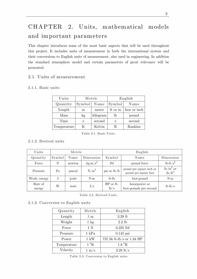
2.1. Units of measurement
2.1.1. Basic units
Units M etric English
Quantity Symbol Name Symbol Name
Length m meter ft or in foot or inch
Mass kg kilogram lb pound
Time s second s second
Temperature K Kelvin R Rankine
Table 2.1. Basic Units.
2.1.2. Derived units
Units M etric English
Quantity Symbol Name Dimension Symbol Name Dimension
Force N newton kg·m/s2
lbf pound force lb·ft/s2
Pressure Pa pascal N/m2
psi or lb/ft pound per square inch or
pound per square foot lb/in
2 or
lb/ft2
Work, energy J joule N·m ft-lb foot-pound N·m
Rate of
energy W watt J/s
HP or ft-
lb/s
horsepower or
foot-pounds per second ft-lb/s
Table 2.2. Derived Units.
2.1.2. Conversion to English units
Quantity M etric English
Length 1 m 3.28 ft
Weight 1 kg 2.2 lb
Force 1 N 0.225 lbf
Pressure 1 kPa 0.145 psi
Power 1 kW 737.56 ft-lb/s or 1.34 HP
Temperature 1 oK 1.8 oR
Velocity 1 m/s 3.28 ft/s
Table 2.3. Conversion to English units.

4
2.2. Earth’s atmosphere
Atmospheric characteristics such as temperature, pressure, density, air speed and
humidity actually vary in a seemingly random way according to different time and
space scales. For aerospace applications a statistic of these variations is used, based on
meteorological data collected over many years.
In almost all atmospheric models the temperature distribution is specified in terms of
segments of a defined and fixed variation of the temperature with altitude. These
mathematical models don’t search a detailed representation of reality (impossible
thing), they are able to establish comparisons between different aircraft models.
Once the temperature gradient value has been defined constant with the altitude for
each segment of the atmosphere (𝜕𝑇(𝑧)/𝜕𝑧 = 𝛽), pressure and density can be deduced
by assuming that the air behaves as an ideal gas.
The mathematical model employed in this case is the International Standard
Atmosphere or ISA [1]:
Standard conditions at sea level
𝑝0 = 101325 𝑃𝑎 → 𝑅𝑒𝑙𝑎𝑡𝑖𝑣𝑒 𝑃𝑟𝑒𝑠𝑠𝑢𝑟𝑒: 𝛿(𝑧) = 𝑝(𝑧)/𝑝0 (2.1)
𝜌0 = 1.225𝑘𝑔
𝑚3→ 𝑅𝑒𝑙𝑎𝑡𝑖𝑣𝑒 𝐷𝑒𝑛𝑠𝑖𝑡𝑦: 𝜎(𝑧) = 𝜌(𝑧)/𝜌0 (2.2)
𝑇0 = 288.15 𝐾 → 𝑅𝑒𝑙𝑎𝑡𝑖𝑣𝑒 𝑇𝑒𝑚𝑝𝑒𝑟𝑎𝑡𝑢𝑟𝑒: 𝜃(𝑧) = 𝑇(𝑧)/𝑇0 (2.3)
𝑎0 = 340.294 𝑚/𝑠 ; 𝜇0 = 17.894 · 10−6𝐾𝑔/𝑚𝑠 ; 𝑔0 = 9.8067 𝑚/𝑠
2
Mathematical model in the Troposphere (𝑧 < 11000 𝑚):
𝜃(𝑧)𝑧<11000 = 𝑇(𝑧)/𝑇0 = (1 − 22.57 · 10−6 · 𝑧) (2.4)
𝛿(𝑧)𝑧<11000 = 𝑝(𝑧)/𝑝0 = (1 − 22.57 · 10−6 · 𝑧)5.256 (2.5)
𝜎(𝑧)𝑧<11000 = 𝜌(𝑧)/𝜌0 = (1 − 22.57 · 10−6 · 𝑧)4.256 (2.6)
Model in the first layer of the Stratosphere (11000 𝑚 < 𝑧 < 20000 𝑚):
𝜃(𝑧)11𝑘𝑚<𝑧<22𝑘𝑚 = 𝑇(𝑧)/𝑇0 = 0.751 = 𝐶𝑜𝑛𝑠𝑡𝑎𝑛𝑡 (2.7)
𝛿(𝑧)11𝑘𝑚<𝑧<22𝑘𝑚 = 𝑝(𝑧)/𝑝0 = 0.223 𝑒−0.15788 (
𝑧1000
−11) (1.8)
𝜎(𝑧)11𝑘𝑚<𝑧<22𝑘𝑚 = 𝜌(𝑧)/𝜌0 = 0.296 𝑒−0.15788 (
𝑧1000
−11)
(2.9)

5
2.2. Important parameters
In model testing of airplanes, missiles or ships in wind tunnels, Reynold’s number,
Froude number and Mach number are accepted scale factors because they contain the
variables which affect parachute performance. The testing models of airplanes, missiles
or ships are rigid bodies mounted in wind tunnels and the data are recorded at different
constant velocities. However the geometry of a deploying parachute undergoes dramatic
changes as compared to the constant geometry of the rigid models. Thereby these scale
parameters (Reynold’s number, Froude number and Mach number) are unsuitable for
parachute deployments because they don’t take into account the change of geometry,
which affect parachutes performance.
Therefore, for any scale parameter to be valid, it must contain those variables that
affect the behaviour of the system. In the case of parachutes, the aforementioned
parameters can be considered suitable if the steady state is considered (with constant
geometry). This parameters will be described below.
In other cases as the parachute deployment and its inflation, in addition to these
parameters will be necessary to take into account other variables that affect the
parachute behaviour. In this case these parameters will be described in subsequent
sections.
Reynolds Number (Re): defines the relationship of mass forces to viscous friction
forces in liquids and gases. It is calculated as
𝑅𝑒 =𝜌 · v · 𝐷0
𝜇=𝑣𝑒𝑙𝑜𝑐𝑖𝑡𝑦 (𝑚/𝑠) · 𝑐ℎ𝑎𝑟𝑎𝑐𝑡𝑒𝑟𝑖𝑠𝑡𝑖𝑐 𝑙𝑒𝑛𝑔𝑡ℎ (𝑚)
𝑘𝑖𝑛𝑒𝑚𝑎𝑡𝑖𝑐 𝑣𝑖𝑠𝑐𝑜𝑠𝑖𝑡𝑦 (𝑚2/𝑠) (2.10)
Reynolds number is an important criterion of viscous effects and allows comparison
of model tests with full-scale flight tests. Table 2.1 shows examples of Reynolds
numbers of various air vehicles.
Reynolds Insect Glider
Aircraft
DC-3
Aircraft
B-747
Drogue
chute
M ain
parachute
6·103
2.5·106
24·106
100·106
50·106
2·106
Table 2.4. Examples of Reynolds numbers for different air vehicles [2].
Mach Number (M): is an important parameter of supersonic flight; it states how
much faster than the speed of sound the air vehicle travels.
𝑀 =𝑣
𝑐𝑆=𝑓𝑙𝑖𝑔ℎ𝑡 𝑣𝑒𝑙𝑜𝑐𝑖𝑡𝑦 (𝑚/𝑠)
𝑠𝑝𝑒𝑒𝑑 𝑜𝑓 𝑠𝑜𝑢𝑛𝑑 (𝑚/𝑠) (2.11)

6
Depending on the configuration of the body, supersonic compressibility effects may
occur in the 0.75-0.85 Mach range, causing local supersonic flow, shock waves, flow
separation, and changes in stability.
Froude Number (Fr): relates the effect of the forces of inertia and the forces of
gravity acting on a fluid.
𝐹𝑟2 =𝑐𝑒𝑛𝑡𝑟𝑖𝑝𝑒𝑡𝑎𝑙 𝑓𝑜𝑟𝑐𝑒
𝑔𝑟𝑎𝑣𝑖𝑡𝑎𝑡𝑖𝑜𝑛𝑎𝑙 𝑓𝑜𝑟𝑐𝑒=
𝑚v2
𝑙𝑚𝑔
=v2
𝐷0𝑔
(2.12)
It is a very useful performance number, since it relates the descent speed in a given
gravitational field to the required size of the parachute canopy.
Mass Ratio (Rm): is a measure of the ratio of air mass enclosed in the inflated
canopy to the payload mass:
𝑅𝑚 =𝜌𝐷0
3
𝑚 (2.13)
The mass ratio is an important parameter during parachute inflation, since the
progressive increase of the parachute diameter increases the value of the mass ratio.
This parameter can be expressed as a function of the Froude number considering
that a vehicle is being retarded by a parachute with a steady descent velocity, and
the drag of the vehicle can be neglected compared to that of the parachute [3].
1
2𝜌𝑣2𝐶𝐷𝑆0 = 𝑚 𝑔 → 𝑣
2 =𝑚𝑔
12𝜌𝐶𝐷
𝜋4𝐷02=
8 𝑚𝑔
𝜋𝜌𝐶𝐷𝐷02 (2.14)
Combining equation (2.14) into equation (2.12):
𝐹𝑟2 =𝑚
𝜌𝐷03
8
𝐶𝐷𝜋=8
𝜋 1
𝑅𝑚𝐶𝐷 → 𝑅𝑚 =
8
𝜋
1
𝐹𝑟2 𝐶𝐷 (2.15)
With this, the speed required to recover a payload can be analysed from these
parameters. Considering a type of parachute with a certain drag coefficient, if it is
desired to have a high speed of descent, the Froude number will be high and
therefore the mass ratio will be small, i.e. the air mass enclosed in the canopy must
be small, and consequently it allows a smaller parachute diameter. On the other
hand, if it is desired to have a low speed of descent, the Froude number will be low,
the mass ratio will be high, and therefore the required air mass will be greater and a
larger parachute diameter will be required.

7
CHAPTER 3. Parachute recovery system and
general considerations
This chapter will discuss the study of the tools needed to evaluate, analyse, select and
design parachute recovery systems. In particular we will focus on providing general
state of the art procedures for high performance parachute design. This includes the use
of aerodynamic and structural analyses to predict parachute inflation, deceleration
forces, parachute stability, or the required weight/volume among other considerations.
First of all it should be mentioned that the term "high performance" parachute may
seem subjective and therefore it is necessary to clarify to what type of parachutes are
concerned. The term high performance parachute includes those that are deployed at
Mach numbers above 0.7 or dynamic pressures above 24 kPa. Parachutes that recover
very heavy payloads at any deployment velocity are also considered to have high
performance. And those parachutes whose weight is small compared to their size and
the drag they produce, are considered to be high performance parachutes.
3.1. Parachute system boundaries
The range of application of the parachutes with respect to speed and altitude is very
wide, since these can be developed specifically for supersonic speeds exceeding Mach 4,
and altitudes above the limits of the atmosphere with dynamic pressures up to 15,000
psi. Figure 3.1 gives an idea of the performance limits of the parachutes developed for
different missions. These boundary limits can move both upward and outward as new
materials and technological advances are introduced.
Figure 3.1. Parachute Performance Envelopes [2].

8
3.2. Parachute design considerations
To select and design a parachute system, the performance characteristics of such
parachute must be considered and known. These performance characteristics can be
many and varied, referring to different criteria such as economic, aerodynamic or
structural scope. The importance of these performance characteristics is different
according to the application of the parachute system and therefore it is not possible to
find general guidelines for designing a parachute with a certain application.
The Table 3.1 lists some possible design criteria:
Reliability Indifference to Damage
Stability Simplicity of Design and
Manufacturing
High Drag Simplicity of Maintenance and
Service
Low Opening Shock Low Acquisition Cost
High Mach Capability Low Life Cycle Cost
Low Weight and Volume Weight Efficiency (𝐶𝐷 · 𝑆)0/𝑊𝑃
Repeatability of
Performance Volume Efficiency (𝐶𝐷 · 𝑆)0/𝑉𝑃
Environmental Adaptability Cost Efficiency (𝐶𝐷 · 𝑆)0/$
Table 3.1. Parachute Design Criteria [2].
Of all these criteria, one could say that reliability is always an important parameter,
since a parachute with a high degree of reliability determines the success or failure of
the mission. For this, it is necessary to analyse and thoroughly review the whole process
that the parachute system performs.
Weight and volume are also very important considerations, which strongly influence the
landing. Normally the structure of a parachute system constitutes 5% of the total
weight of a light vehicle, or 3-4% for heavier vehicles.
Parachute selection frequently begins with the stability requirement. This requirement
limits the oscillation of the parachute, so that a high level of stability automatically
eliminates many types of high-drag parachutes or involves the use of parachute
clusters.
The drag coefficient is an important parameter in the selection of the parachutes in the
final descent. This parameter influences the weight-efficiency ratio criteria, which shows
how much Drag area (𝐶𝐷 · 𝑆)0, is produced per kilogram of parachute 𝑊𝑝.
Repeatability and maintenance are factors that directly influence the cost of the
parachute system.

9
Figure 3.2. Principal components of a parachute [4]
Table 3.2 shows a guide to evaluate the importance of some parachute performance
characteristics according to different applications. Each designer can use different rating
values based on the specific requirements of a particular application.
PERFORM ANCE
CHARACTERISTICS
APPLICATION
Spacecraf
landing
Airborne
troops
Aircraft
landing Ordnance
Aerial
resupply
Reliability of operation 3 3 3 3 2
Repeatability of performance 2 2 2 3 1
Reuse 0 3 0 0 3
Low weight and volume 3 2 3 2 1
Stability 2 2 2 3 2
High drag 2 2 2 2 3
Low opening forces 1 3 2 2 3
Low maintenance/service 1 3 2 2 3
Cost 1 2 2 2 3
3= high importance
2= medium importance
1=low importance
0= not applicable
Table 3.2. Comparative Rating of Performance Characteristics for Various Parachute
Systems Applications [2].
3.3. Parachute structural analyses
3.3.1. Basic description of H igh-performance Parachutes
Before discussing specific high-performance
parachute configurations in detail, it is
necessary to identify their principal parts
and define the parameters and
nomenclature used to measure their
performance. Figure 3.2 illustrates the basic
features of a parachute:
The canopy is the cloth surface that
inflates to a developed aerodynamic shape
to provide the lift, drag and stability
needed to meet performance requirements.
Canopies are formed from a number of
gores bounded on each side by a radial
seam (on the top edge by the vent band
and on the bottom edge by the skirt band).

10
The suspension or shroud lines transmit the force form the canopy to the payload,
either directly or through risers attached below the convergence point of the
suspension lines to the body. This point of convergence of all suspension lines is called
the confluence point.
The crown is the region of the canopy above the major diameter of the inflated shape,
and the small circular opening at the centre of the crown is called the vent, which
serves to simplify fabrication and provides flow-through relief for the initial surge of air
when it impacts the canopy at the start of inflation.
The payload may be fastened directly to the lower end of the risers, but if there is
reason to suspend it lower, extension lines are used. If it is desirable that the payload
can be free to turn independently of the parachute, a swivel may be placed in the
suspension system anywhere below the risers.
The open region at the apex of the canopy is the vent (𝑫𝒗). The portion that extends
below the major diameter of the inflated canopy shape to the leading edge of the
canopy is the skirt. On the skirt it can be measured the projected diameter (𝑫𝒑) of the
inflated parachute, but since this latter is a function of the parachute’s inflated shape
and the load that it is carrying, parachutes are usually described by their nominal
diameter (𝑫𝟎), which is the effective diameter of a circle whose area is the nominal
area (𝑺𝟎). The nominal area is the actual three-dimensional canopy surface area,
computed as the sum of the gore areas.
Another reference dimension of parachutes is the constructed diameter (𝑫𝒄), the
diameter of the parachute measured along the radial seam when projected on a planar
surface. Another important parameter that defines the parachute geometry is the
suspension line length (𝒍𝒆), the distance from the canopy skirt to the confluence point.
In the Figure 3.3 it can be observed the different parameters mentioned:
Figure 3.3 Geometric parameters of a parachute [4].
Dc Dv Dp
hp
le
11
A Table with typical high-performance parachute with most of the shape factors,
general aerodynamic characteristics and applications of the parachutes are listed in the
Appendix A [5]. Numerical values for inflated shape factor (𝐷𝑐/𝐷0) and drag
coefficient (𝐶𝐷0) represent a range of values influenced by geometric factors and fluid
dynamic parameters such as: canopy size, canopy porosity, Mach number, suspension
line length, material, air density or dynamic pressure. The influence of these factors will
be discussed in subsequent sections.
3.3.2. Parachute Deployment
Parachute deployment denotes the sequence of events that begins with the opening of a
parachute compartment attached to the body to be recovered and continues with
extraction of the parachute until the canopy and suspension lines are stretched behind
the body and the parachute is ready to start the inflation process.
This deployment is associated with a mass shock (snatch force) created by the
acceleration of the mass of the parachute to the velocity of the body to be recovered.
Therefore, the task of a good deployment system is to limit the mass shock by
controlling the parachute deployment process and providing means for progressive
incremental acceleration of all parts of the parachute.
Parachute and riser should be stored in a textile envelope for protection during
deployment and to ensure a controlled deployment that keeps tension on all parts of
the parachute and riser. The textile envelope, called the deployment bag, usually have
separate compartment for the canopy, suspension lines and for the riser. These
compartments allow an incremental deployment sequence, thereby maintaining order
and tension on all parts of the deployment parachute assembly.
There are several deployment methods, that fit better or worse according to the needs
required by the operation.
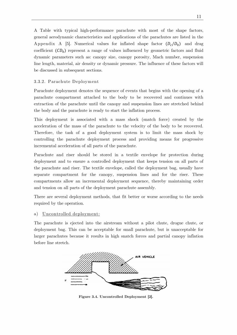
a) Uncontrolled deployment:
The parachute is ejected into the airstream without a pilot chute, drogue chute, or
deployment bag. This can be acceptable for small parachute, but is unacceptable for
larger parachutes because it results in high snatch forces and partial canopy inflation
before line stretch.
Figure 3.4. Uncontrolled Deployment [2].

12
b) Semicontrolled deployment:
Semicontrolled deployment uses a pilot chute for extracting the main parachute. It
works with medium-sized parachutes at low velocities, but at high speeds, the pilot
chute can be powerful enough to cause high snatch loads. Partial canopy inflation
before canopy stretch can also occur with this deployment.
c) Static-Line deployment:
A static line is attached on one side to the air vehicle and on the other side to the
parachute assembly. First open the parachute pack and then pull the parachute out of
its deployment bag. It is a typical method used by paratroopers and is limited to
aircraft speeds of about 240 km/h.
Figure 3.5. Pilot Chute Deployment [2].
Figure 3.6. Parachute Static-Line Deployment [2].

13
d) Controlled deployment:
It is the basic deployment method for all parachute used for the recovery and
retardation of air/space vehicles, ordnance items and high-speed payloads.
Controlled parachute deployment starts with the forced ejection of a parachute
compartment cover that pulls a pilot chute away from the air vehicle. The sequence in
the deployment of the parachute assembly is: riser, suspension lines and canopy. The
deployment bag of the main parachute contains compartments that ensure a controlled
deployment with tension on all parts of the parachute.
3.3.3. Pilot Chutes
Pilot chutes are used to deploy large parachutes from their storage packs or containers
into good airflow behind the vehicle. Its task consists in first extracts the parachute
pack from the vehicle compartment and then deploys the main parachute form its
deployment bag. For achieve this, some requirements, based on experience, can be
defined for pilot chutes:
- Pilot chutes must open quickly and reliably.
- Pilot chutes must be stable and must have sufficient drag to pull the main
parachute pack away from the payload and extract the main parachute.
- The recommendation is to eject the pilot chute to a distance equivalent to at
least four, and, if possible, six times the forebody diameter behind the vehicle.
- As a rule, the pilot chute extraction force should be equal to or larger than four
times the weight of the parachute assembly to be extracted.
Values of drag coefficients and opening-force coefficients for typical pilot chutes are
shown in Table 3.3:
Square box 0.60 2.0
Ribbon, conical 0.52 1.3
Ringslot 0.60 1.4
Guide surface 0.42 2.0
Pilot Chute type Drag Coefficient, Opening-force coefficient,
Table 3.3. Pilot Chute Drag and Opening-Force Coefficients [2].
Figure 3.7. Controlled Parachute Deployment Concpet [2].

14
3.3.4. Parachute Stress Analysis
Since textiles are the primary materials used in parachutes, their characteristics must
be considered in establishing design factors and in dimensioning the various elements of
the parachute assembly. Textiles are used for cloth or ribbons of the parachute canopy;
for webbings, lines and tapes for suspension lines and canopy reinforcements; and for
some parts of deployment bags and related components. These textile components are
affected much more than are metals by such environmental factor as temperature,
humidity, radiation, chemicals or aging; and such mechanical factors as abrasion,
handling and packing.
It is very difficult to determine the load and stress distribution for a variable-geometry,
variable-velocity inflating canopy. Mullins and Reynolds developed a computerized
system for calculation the stresses in ribbon parachutes. This method, called CANO
program, was modified and improved by the University of Minnesota and the Sandia
National Laboratories [6]. The improved version of the CANO program published by
the Sandia National Laboratories was called Canopy Load Analysis (CALA) [7].
Prior to the CANO program, three methods were developed that give a good
approximation for determining the maximum force that could experiences the canopy.
Because this maximum force occurs during the canopy filling process, these three
methods will be clarified in the section related to inflation of the canopy, since some
concepts of this process should be explained before to understand the methods.
3.3.5. Textile M aterials
It is not the purpose to provide a detailed analysis of the complex area of textiles and
fabrics, but rather to provide a general overview of the textiles used in the design and
manufacture of parachute assemblies.
The two primary groups of textiles are those of natural fibers and those of man-made
fibers. Natural fibers include wool, cotton, silk, flax and many others, but only silk and
cotton are of interest to parachute design. Man-made fibers are classified by their
origins. Mineral fibers, the only nonorganic fibers, include glass fiber and metal thread
used in woven metals. All other man-made fibers are based on cellulose, protein, or
resin composites. The cellulose group includes rayon, and the protein and resin groups
include nylon, dacron or Kevlar.
In the Appendix B [2] the main characteristics of the mentioned textile materials are
listed in a table. Of all these textile materials, it is important to mention that Kevlar
has become very used as high-tenacity material for parachute assemblies. Kevlar is
about 2.5 to 3 times stronger than nylon and is considerably more heat resistant.
Hybrid parachutes using nylon canopies and Kevlar suspension lines, risers and canopy
tapes can reduce weight and volume by 25% to 40%, depending on the amount of
Kevlar used.
15
3.3.6. Parachute Recovery System Weight and Volume
The relationship of weight and volume can be expressed by the amount of parachute
weight that can be packed into 1 cubic foot of volume. This introduces the importance
of pressure packing. The higher the pressure, the more weight can be stowed in a given
space. Although nylon parachutes and all-Kevlar parachutes can be packed with similar
pressures, Kevlar parachutes increase the pack density because of the 26% higher
specific weight of Kevlar, as it can be seen in Appendix B.
There are mainly four methods for calculating the weight of a parachute recovery
system: the preliminary design method [2]; the drawing method [2]; the TWK method
[2]; and the Keneth E. French Method [8].
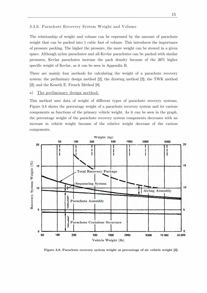
a) The preliminary design method:
This method uses data of weight of different types of parachute recovery systems.
Figure 3.8 shows the percentage weight of a parachute recovery system and its various
components as functions of the primary vehicle weight. As it can be seen in the graph,
the percentage weight of the parachute recovery system components decreases with an
increase in vehicle weight because of the relative weight decrease of the various
components.
Figure 3.8. Parachute recovery system weight as percentage of air vehicle weight [2].

16
As a simple and quick general rule, deployment bags weigh 5 to 6% of the parachute
system, and deployment bags plus pilot chute add 3 to 5%. First-stage drogue-chute
assemblies will weigh from 25 to 40% of the main parachute weight depending on the
deployment dynamic pressure and riser length. Parachute cluster have 5 to 10% higher
weight than a single parachute of equal drag area because of the loss in drag caused by
cluster interference.
This is not a very precise method, especially if the required parachute differs
significantly from the parachutes considered in the graphs. In any case, it allows us to
have an approximate idea of the weight of the parachute system.
b) The drawing method:
If detailed drawings with material lists are available, the weight of the parachute
assembly can be determined from the material and hardware specifications. Experience
shows that this method is usually precise because the estimated weight is frequently
about 5% higher than the weight of the manufactured assembly.
c) The TKW method:
If no detailed drawing is available, but the primary dimensions of the parachute are
known, the following method will give good weight data. The weight of a parachute can
be written in following form:
𝑊𝑃 = 𝑆0 · 𝑤𝑐 + 𝐷0/2 · 𝑁𝐺 · 𝑤𝑅𝑇 · 𝐹𝑅𝑇/1000 + 𝑁𝑆𝐿 · 𝐿𝑆 · 𝑤𝑆𝐿 · 𝐹𝑆𝐿/1000 (3.1)
Where:
- 𝑊𝑃 is the weight of the parachute (lb or kg).
- 𝑆0 is the surface area of the finished canopy (ft2 or m
2).
- 𝑤𝑐 is the specific canopy weight (lb/ ft2 or kg/m2).
- 𝑁𝐺 is the number of radials (gores) in the canopy.
- 𝑤𝑅𝑇 is the specific weight of the radial tape (lb/ft/1000-lb).
- 𝐹𝑅𝑇 is the strength of the radial tape (lb or kg).
- 𝑁𝑆𝐿 is the number of suspension lines.
- 𝐿𝑆 is the length of suspension lines (ft or m).
- 𝑤𝑆𝐿 is the specific weight of suspension lines (lb/ft/1000-lb).
- 𝐹𝑆𝐿 is the strength of suspension lines (lb or kg).
In this formula 𝑆0, 𝑁𝐺 , 𝑁𝑆𝐿 , 𝐿𝑆, 𝐹𝑅𝑇 , 𝐹𝑆𝐿 are known preliminary design data.

17
d) The Kenneth E. French method:
This method is only used to estimate the weight of the parachute canopy in a fast but
effective way in preliminary design tasks, where the riser, deployment bag, and special
attachment link weights are excluded. Kenneth E. French [8] collected the weight of 59
different parachutes with conventional materials as nylon, including different sizes of
Flat solid, Ext. skirt, Ringslot, Flat ribbon and Conical ribbon. Most of them were of a
relatively conventional construction with 𝐿𝑆/𝐷0~1 and 𝑁𝑆𝐿~𝐷0. Figure 3.9 shows
weight versus 𝑁𝑆𝐿𝑃𝑠𝐷0 on log-log scales for these parachutes, where 𝑃𝑠 (Newtons), is the
rated ultimate strength of suspension line.
The straight line shown in Figure 3.9 is:
𝑊(𝑘𝑔) = 1.9 · 10−5(𝑁𝑆𝐿𝑃𝑠𝐷0)0.96 (3.2)
The data scatter in Figure 3.9 appears due as much to variations within each specific
type of chute as to type-to-type variations. Thus, the incorporation of all types of chute
in one graph appears valid.
The nominal weight value of equation (3.2) multiplied by 1.21 should provide a fairly
conservative maximum weight for estimating purposes. For most chute applications, if
there are small changes in deployment conditions 𝑁𝑆𝐿𝑃𝑠 ∝ 𝐹𝑋. This relationship can be
used to obtain the variation in 𝑊 for small variations in 𝑞 and 𝐷0.
Figure 3.9. Parachute weight vs NPsD0 [8].
18
3.4. Parachute aerodynamic analyses
3.4.1. Stability of parachute systems
Stability is the tendency of a body to return to an equilibrium position after a
displacement of that position. Such stability must be considered both from a static and
from a dynamic point of view.
Thus, a system is considered to be “statically stable” when in that system a moment
develops in the direction that allows restoring equilibrium. In addition, if a system
presents static stability on one of its axis, it doesn’t necessarily mean that it is stable
on any other axis, and therefore it is important to define the axis on which the stability
of the system is considered. The criterion that defines the static stability of a parachute
in pitch can be expressed mathematically by the variation of the pitch moment with
respect to the angle of attack:
𝜕𝑀𝐺𝜕𝛼
< 0 → 𝑠𝑡𝑎𝑏𝑙𝑒
𝜕𝑀𝐺𝜕𝛼
= 0 → 𝑛𝑒𝑢𝑡𝑟𝑎𝑙𝑙𝑦 𝑠𝑡𝑎𝑏𝑙𝑒
𝜕𝑀𝐺𝜕𝛼
> 0 → 𝑢𝑛𝑠𝑡𝑎𝑏𝑙𝑒
(3.3)
On the other part the “dynamic stability” refers to the damping of the continuous
movement of a body as a consequence of the frictional forces and the gravitational
component. But the fact that a body is dynamically stable is not enough, because it is
really important that the time to reduce its oscillation to an external disturbance is
adequate and thus avoid too high amplitudes of oscillation.
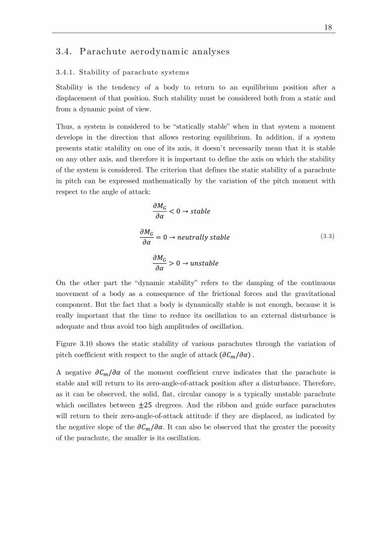
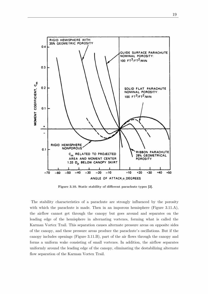
Figure 3.10 shows the static stability of various parachutes through the variation of
pitch coefficient with respect to the angle of attack (𝜕𝐶𝑚/𝜕𝛼) .
A negative 𝜕𝐶𝑚/𝜕𝛼 of the moment coefficient curve indicates that the parachute is
stable and will return to its zero-angle-of-attack position after a disturbance. Therefore,
as it can be observed, the solid, flat, circular canopy is a typically unstable parachute
which oscillates between ±25 dregrees. And the ribbon and guide surface parachutes
will return to their zero-angle-of-attack attitude if they are displaced, as indicated by
the negative slope of the 𝜕𝐶𝑚/𝜕𝛼. It can also be observed that the greater the porosity
of the parachute, the smaller is its oscillation.
19
The stability characteristics of a parachute are strongly influenced by the porosity
with which the parachute is made. Then in an imporous hemisphere (Figure 3.11.A),
the airflow cannot get through the canopy but goes around and separates on the
leading edge of the hemisphere in alternating vortexes, forming what is called the
Karman Vortex Trail. This separation causes alternate pressure areas on opposite sides
of the canopy, and these pressure areas produce the parachute’s oscillations. But if the
canopy includes openings (Figure 3.11.B), part of the air flows through the canopy and
forms a uniform wake consisting of small vortexes. In addition, the airflow separates
uniformly around the leading edge of the canopy, eliminating the destabilizing alternate
flow separation of the Karman Vortex Trail.
Figure 3.10. Static stability of different parachute types [2].

20
3.4.2. Parachute inflation process
Parachute inflation is defined as the time interval from the instant the canopy and lines
are stretched to the point when the canopy is first fully inflated. Figure 3.12 shows the
phases of the canopy inflation.
Figure 3.12. Parachute Canopy Inflation Process [2].
Case A) Imporous canopy,
instability caused by side
force N.
Figure 3.11. Relationship of Ariflow and Stability depending on porosity [2].
Case B) Porous canopy,
no side force, no unstable
moment.
B)
A)

21
The canopy filling process begins when canopy and lines are stretched and when air
begins entering the mouth of the canopy (a). After the initial mouth opening, a small
ball of air rushes toward the crown of the canopy (b). As soon as this initial air mass
reaches the vent (c), additional air starts to fill the canopy form the vent toward the
skirt (d). The inflation process is governed by the shape, porosity, size of the canopy
and by air density and velocity at the start of inflation. Inflation is slow at first but
increases rapidly as the mouth inlet of the canopy enlarges (e) and the canopy reaches
its first full inflation (f). And finally most solid textile canopies overinflate and
partially collapse because of the momentum of the surrounding air (g).
During this process it is important to consider that the amount of air toward the
canopy vent at point (b) should be small to avoid a high-mass shock when the air
bubble hits the vent of the parachute. Furthermore, the inflation of the canopy should
occur axisymmetrically to avoid overstressing of individual canopy parts. And the
overinflation phenomena after the first initial opening should be limited to avoid delay
in reaching a stable descent position.
Several methods have been developed to obtain quantitative values for opening time
and force. These methods vary from easily usable empirical models to models whose
comparison is as complex as they are almost useless for parachute designers.
a) Canopy inflation time
Knowledge of the canopy filling time, defined as the time from canopy stretch to the
first full open canopy position, is important. Over the years many authors have
developed numerous methods to calculate this filling time considering different types of
parachutes.
Mueller [9] y Scheubel [10] assumed, based on the continuity law, parachutes should
open within a fixed distance, because a given conical column of air in front of the
canopy is required to inflate the canopy. This fixed distance is proportional to a
parachute dimension such as the projected diameter, 𝐷𝑝. Therefore the filling distance
for a specific parachute can be defined as:
𝑠𝑓 = 𝑛 · 𝐷𝑝 (3.4)
Figure 3.13. Filling distance of a parachute canopy [2].
22
Because the parachute diameter, Dp, is variable, the fixed nominal diameter, Do, is
used to calculate canopy filling time [2]:
𝑡𝑓 =𝑛 · 𝐷0𝑣
(3.5)
Where:
- 𝐷0 is the nominal parachute diameter.
- 𝑣 is the velocity at line stretch.
- 𝑛 is a constant typical for each parachute type, indicating the filling distance
as a multiple of 𝐷0.
This basic fillig-time equation was extended by Kancke, Fredette, Ludtke and others
[11, 12], providing good results.
Ribbon Parachute (Knacke)
𝑡𝑓 =𝑛 · 𝐷00.9 𝑣
; Where n = 8 for Ribbon parachutes (3.6)
Ribbon Parachute in high-speed tests (Fredette)
𝑡𝑓 =0.65 𝜆𝑇 · 𝐷0
𝑣 (3.7)
Where 𝜆𝑇 is the total canopy porosity expressed as a percent of the canopy
surface area.
Solid Flat Circular Parachute (Wright Field)
𝑡𝑓 =𝑛 · 𝐷00.85 𝑣
(3.8)
Where n=4 for standard porosity canopies, and n=2.5 for low porosity canopies.
Cross Parachute (Silver Spring)
𝑡𝑓 =(𝐶𝐷𝑆)𝑝 · 𝑛
𝑣0.9 Where n=8.7 (3.9)
Reefed Parachutes: Parachute reefing is a method that permits the
incremental opening of a parachute canopy, or restrains the parachute canopy
form full inflation or overinflation. This method consists mainly of two stages:
reefing the parachute provides a temporarily high rate of descent with a low
drag area that permits a more accurate drop form high altitude; and disreefing
the parachute provides a low-impact velocity.
𝑡𝑓1 =𝑛1 · 𝐷0𝑣𝑠
· [(𝐶𝐷𝑆)𝑅(𝐶𝐷𝑆)0
]
12
𝑎𝑛𝑑 𝑡𝑓2 =𝑛2 · 𝐷0𝑣𝑅
· [(𝐶𝐷𝑆)0 − (𝐶𝐷𝑆)𝑅
(𝐶𝐷𝑆)0]
12
(3.10)

23
Where:
- 𝑡𝑓1 and 𝑡𝑓2 are the reefed and disreefed filling times.
- 𝑣𝑠 and 𝑣𝑅 are the velocities at line stretch and at disreef.
- (𝐶𝐷𝑆)𝑅 and (𝐶𝐷𝑆)0 are the reefed- and full-open drag areas.
- 𝑛1 is 10 for ribbon parachutes or 8 for ringsail parachutes.
- 𝑛2 is 6 for ribbon parachutes or 2 for ringsail parachutes.
Some types of ribbon parachutes have been opened in the velocity range of up to Mach
4, where the canopy filling time at supersonic speed can be considered constant,
because the canopy operates behind a normal shock. In later sections, we will focus on
the applications of these supersonic parachutes.
b) Parachute drag-area increase during inflation process
The parachute drag area, (𝐶𝐷𝑆)𝑃, increases from 0 to 100% during canopy inflation.
This drag-area-versus-time curve normally has a specific shape for each canopy type
and it may be drawn out or compressed by reefing, changes in porosity distribution or
other means. However, the basic configuration of the curve is maintained for a
particular type of parachute, as the Figure 3.14 and Figure 3.15 show:
This drag-area could be called more precisely “dynamic drag area”, because it is
obtained from the measured instantaneous force over the instantaneous dynamic
pressure. Therefore it includes characteristics that affect the opening process, such as
apparent mass and altitude density.
Data on drag-area-versus-time increase for the various parachute types are important
for establishing the force-trajectory-time analysis of parachute recovery systems.
Figure 3.14. Typical Drag-Area-Versus-Time Increase for Various Parachute Types [2].
Figure 3.15. Typical Drag-Area-Versus-Time Increase for Reefed Parachutes [2].

24
c) Effect of canopy loading, 𝑾/(𝑪𝑫𝑺)𝑷, on parachute opening forces
To analyse the effect of canopy loading, two general types of behaviour can be taken
into account: parachutes opened under conditions of infinite mass and parachutes
opened under finite mass conditions.
When infinite mass condition is considered, the velocity doesn’t decay during parachute
inflation and the parachute acts as if it were attached to an infinite mass. This
condition is characteristic of high canopy loading. And when finite mass condition is
considered, the velocity during the parachute opening decreases substantially and is
representative of low canopy loading.
An additional typical difference between infinite and finite mass conditions is the
location of the so called peak opening force, 𝑭𝒙. For a parachute opened under
infinite mass conditions, or high canopy loading, the peak opening force occurs at the
first full canopy inflation. But the peak opening force of a parachute opened at a finite
mass condition will occur long before the parachute canopy is fully open. In the Figure
3.16 it is shown the different force-time diagrams.
Fs: Snatch Force ; Fx: Peak Opening Force ; Fc: Steady-state Force ; ti: Inflation Time
Figure 3.16. Force-versus-Time diagrams for infinite and finite mass conditions [3].

25
Defining the opening-force coefficient, 𝑪𝒙, as the relationship of the peak opening force,
𝐹𝑥, to the steady-state drag force, 𝐹𝐶, the equation for the parachute force can be
written:
𝐹𝑥 = 𝐹𝑐 · 𝐶𝑋 · 𝑋1 = (𝐶𝐷𝑆)𝑃 𝑞 · 𝐶𝑋 · 𝑋1 (3.11)
Where:
- (𝐶𝐷𝑆)𝑃 is the drag area of the fully open parachute.
- 𝑞 is the dynamic pressure.
- 𝐶𝑋 is the opening force coefficient at infinite mass. Its value depends on each type
of parachute.
- 𝑋1 is the opening-force-reduction factor. Its value is 1.0 for a parachute opened at
the infinite mass condition, and is as low as 0.02 for a low canopy loading.
d) M ethods for calculating parachute opening forces
The most common methods for calculation parachute opening forces are three. The
Method 1, the 𝑊/(𝐶𝐷𝑆)𝑃 method [20], is fast but should be used for preliminary
calculations only. Method 2, the Pflanz method [23], is mathematically exact and
provides good results within certain application limits. Method 3, the computerized
force-trajectory-time method [24], gives good results with no limitations. However, all
three methods require knowledge of certain parachute and opening-process
characteristics.
In this case, of all these methods, the second one will be detailed below, since for a
preliminary design it is considered more accurate than the first method and less
complicated than the third method.
The Pflanz method is based on the following concept: a body of known fixed weight and
velocity is decelerated along a vertical flight path by an aerodynamic drag device whose
drag area increases form a small value to 100% in a known, mathematically definable
form. This method is mathematically exact, however, no drag area overshoot is
included at the start of the reefed or disreef inflation cycle.
In this method it is defined a dimensionless parameter, which is obtained from known
data and is called ballistic parameter, 𝑨.
𝐴 =2 𝑊
(𝐶𝐷𝑆)𝑃 𝜌 𝑔 𝑣 𝑡𝑓 (3.12)
Where:
- 𝐴 is the ballistic parameter.
- 𝑊 is the system weight.
- (𝐶𝐷𝑆)𝑃 is the drag area.
- 𝑔 is the acceleration of gravity.
- 𝜌 is the air density at altitude of
parachute inflation.
- 𝑣 is the velocity of descend.
- 𝑡𝑓 is the canopy inflation time.

26
𝑊,𝑔 and (𝐶𝐷𝑆)𝑃 are fixed values for each specific application. The filling time 𝑡𝑓 can
be calculated by the methods given in section 3.4.2.a, and the velocity of descend 𝑣 can
be measured. Before calculating the ballistic parameter, it is necessary to determine the
shape of the drag-area-versus-time curve, that is denote by the letter n: the n=1 curve
is a straight line, typical for ribbon and ringslot parachutes; the concave curve, n=2, is
representative of solid cloth, flat circular, conical and extended-skirt parachutes; and
the convex form is for reefed inflation of extended-skirt parachutes. Once the value of
the ballistic parameter is calculated, the force factor 𝑋1 can be obtained from the graph
in Figure 3.17.
In the case of the opening-force coefficient, the table of the Appendix A presents values
of 𝐶𝑋, for a variety of unreefed parachute types operating under infinite mass inflation
conditions; these values range from a high of 1,8 for a solid flat canopy to a low of 1.0
for a hemisflo ribbon canopy. Since there is little drag overshoot for a reefed parachute,
a value of 𝐶𝑋 of 1.0 should be used for inflation to a reefed stage.
Finally, the opening force of the parachute can be calculated using the equation (3.11)
Figure 3.17. Opening-Force Reduction Factor versus Ballistic Parameter [2].
27
3.4.3. Altitude effects
A parachute dropped at a certain speed but different altitudes may have greater
opening forces at higher altitudes than at low altitudes. This phenomenon occurs in
particular when the parachute system has a low canopy loading, which causes the value
of the ballistic parameter to take small values in the range between 0-10. As it can be
seen in the graph of Figure 3.17, this range of values results in a highly variable
opening force reduction factor, which can take lower values when the altitude is low or
higher values when the altitude is higher. Consequently, as we saw in the equation
(3.11), if the force reduction factor varies, the opening force also varies proportionally.
However, we can also observe in the graph of Figure 3.17 that for a range of values of
the ballistic parameter between 10 and 1000, the value of the opening force reduction
factor hardly varies with the altitude, and therefore the opening forces also do not vary.
In this case, this phenomenon occurs when the loading canopy is high.
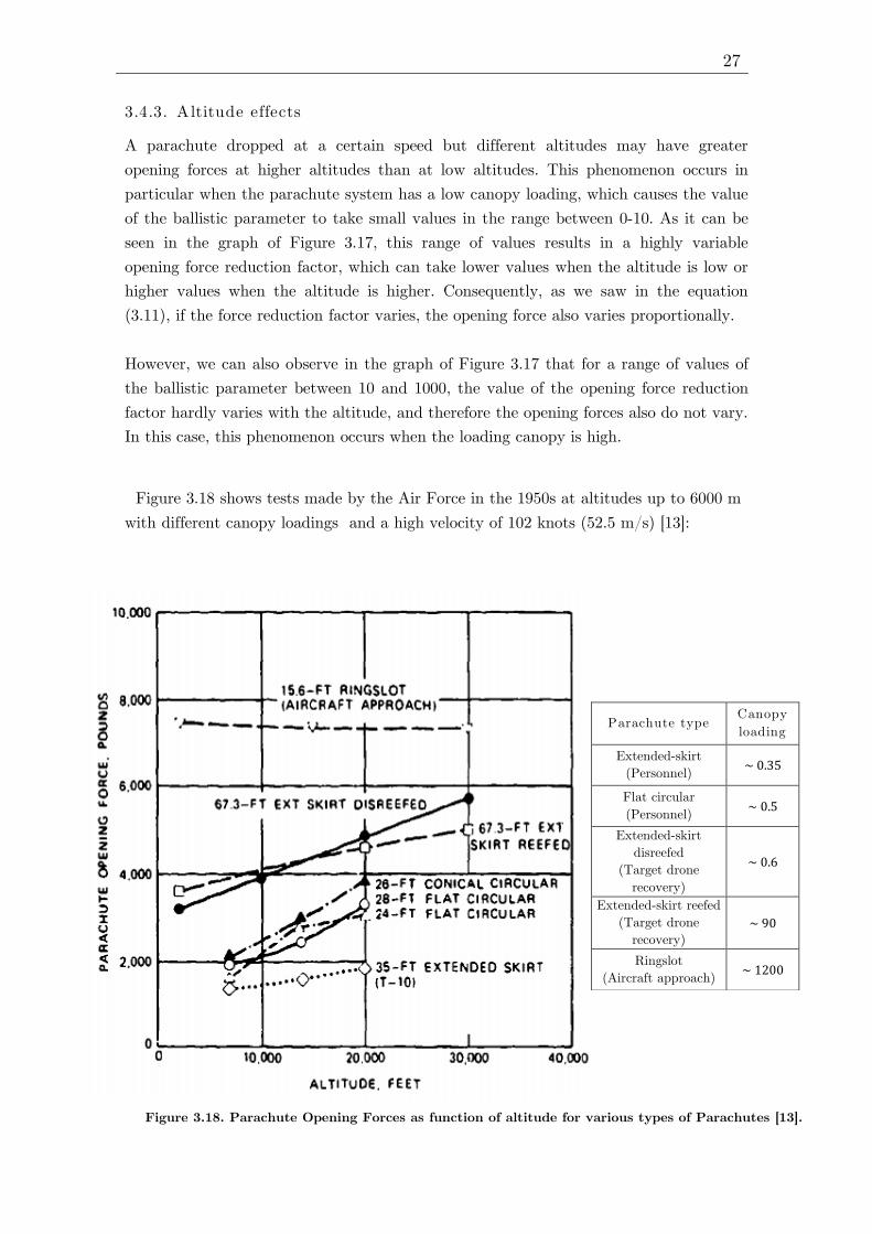
Figure 3.18 shows tests made by the Air Force in the 1950s at altitudes up to 6000 m
with different canopy loadings and a high velocity of 102 knots (52.5 m/s) [13]:
Parachute type Canopy
loading
Extended-skirt
(Personnel) ~ 0.35
Flat circular
(Personnel) ~ 0.5
Extended-skirt
disreefed
(Target drone
recovery)
~ 0.6
Extended-skirt reefed
(Target drone
recovery) ~ 90
Ringslot
(Aircraft approach) ~ 1200
Figure 3.18. Parachute Opening Forces as function of altitude for various types of Parachutes [13].
28
3.4.4. Porosity effects
The porosity of parachute canopies influences parachute characteristics and parachute
performance. For parachute canopies manufactured form solid fabric, the nominal
porosity was defined by Heinrich [27] as the volumetric airflow per unit area of material
per unit of time (ft3/ft
2/s is commonly used). For slotted canopies such as ribbon,
ringslot and ringsail parachutes, geometric porosity is defined in percent as the ratio of
all open areas to the total canopy area (typical values are in the 10 to 35 % range).
Porosity affects parachute drag, stability and opening forces. The porosity increase
makes the opening forces and oscillation smaller, that is desirable, but also makes the
drag smaller, that is generally undesirable.
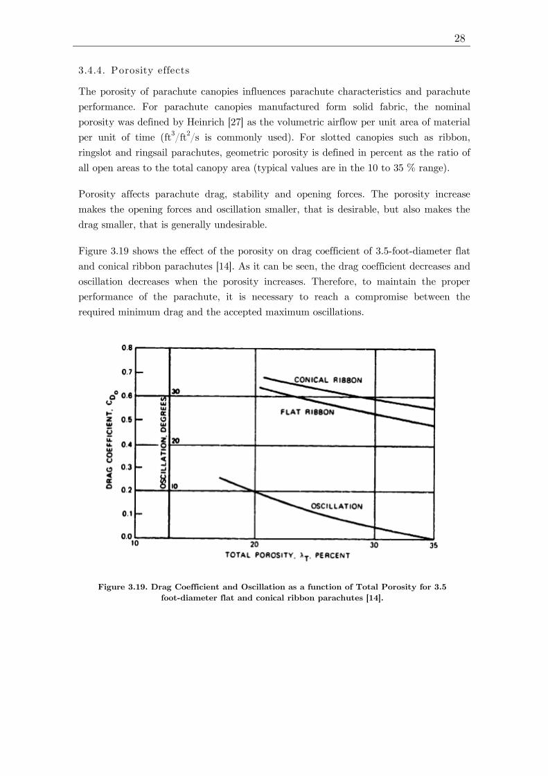
Figure 3.19 shows the effect of the porosity on drag coefficient of 3.5-foot-diameter flat
and conical ribbon parachutes [14]. As it can be seen, the drag coefficient decreases and
oscillation decreases when the porosity increases. Therefore, to maintain the proper
performance of the parachute, it is necessary to reach a compromise between the
required minimum drag and the accepted maximum oscillations.
Figure 3.19. Drag Coefficient and Oscillation as a function of Total Porosity for 3.5
foot-diameter flat and conical ribbon parachutes [14].

29
3.4.5. Canopy shape and pressure distribution
The inflated shape of a parachute canopy depends on the type and geometric design of
the canopy, on the canopy porosity, and on the suspension-line length. These factors
are responsible for generating a certain balance of internal pressures forces and the
tension in the suspension lines, which directly affects the instant shape of the canopy.
A decrease in canopy porosity and an increase in suspension-line length are the prime
reasons for an increase in inflated canopy diameter and associated increase in drag
coefficient. In Figure 3.20 it can be observed an example of the variation of the shape
respect to the increase of canopy porosity and Figure 3.21 shows the canopy diameter
variation respect to the line-ratio increase (𝑙𝑒/𝐷0) .
In regard to the pressure distribution over the parachute canopy is important to know
the inflation characteristics of the canopy in order to determine canopy stresses. The
desirable condition for parachutes is to keep a uniform airflow separation around the
leading edge of the canopy and a uniform wake behind the canopy for obtaining high
drag and good stability. As Figure 3.22 shows, the airflow in front of the canopy is
decelerated to zero at the stagnation point (I) . Behind the stagnation point, turbulent
airflow occurs, resulting in a high static pressure inside the parachute canopy compared
to the static pressure in the undisturbed flow of the free airstream around the canopy.
The airflow around the edge of the canopy is accelerated by the compression of the
streamlines, causing a negative pressure difference on the outside of the canopy. The
positive inside pressure difference and the negative outside pressure difference form a
strong pressure gradient outwards that keeps the canopy inflated.
Figure 3.22.
Airflow and pressure
distribution around a
parachute canopy. [2]
Figure 3.21. Parachute with constant porosity and
Suspension line ratios of 1.0, 1.5 and 2.0 [2].
Figure 3.20. Parachute canopies with constant
suspension-line ratio and porosities from 15 to 30%

30
3.5. Clustering of parachutes
A parachute cluster consists of two or more parachutes used to stabilize, decelerate or
lower a payload. The use of this clustering basically depends on the mission, which
must take into account both the advantages and disadvantages that entails.
On the one hand several small parachutes are easier to fabricate, store, maintain,
handle and retrieve than a single large parachute. During its performance, they also
have less probability of a catastrophic system failure than a single one and provide a
stable descent even when using individual, high-drag, unstable parachutes. Another
important advantage during its performance is that a parachute cluster has a shorter
filling time than a single large parachute.
On the other hand however, it is impossible to obtain a perfectly synchronized opening
of all parachutes in a cluster. For this reason each parachute in the cluster must be
designed to handle the maximum individual load. Therefore, the total strength of the
parachutes in a cluster and their associated weight and volume are higher than the
weight and volume of a single large parachute of equivalent drag area and because of
the interference and systems geometry, they also experience a reduction in drag,
although its effect is less aggressive.
3.5.1. Loss of Drag in Cluster Applications
Parachutes combined into clusters suffer a reduction in drag because of the geometry of
the cluster system, which forces parachutes to fly at a large angle of attack. However
this problem can be reduce using longer suspension lines to decrease the individual
angle of attack and thereby increases the cluster drag. Another reason of reduction in
drag also happens because of mutual interference, but this reason is less aggressive than
the previous one.
Figure 3.23. Typical Parachute Cluster Arrangement [2].

31
Figure 3.24 shows a group of parachutes of different types and different sizes, whose
drag coefficient decreases as the number of parachutes in the cluster increases.
3.5.2. Synchronization problems
The problems of synchronization can occur if one of the parachutes of the cluster
inflates ahead of the others, since the velocity and dynamic pressure decreased so
rapidly that the remaining pressure is not enough to inflate the lag parachutes. This is
considered a catastrophic failure because the early inflated parachutes can be
destructed by the supported overload.
To avoid this problem the reefing technique is used. Reefing the individual parachutes
in the cluster allows all parachutes to obtain an initial inflation followed by a
reasonably uniform full inflation and inflation forces.
Figure 3.24. Drag loss in Parachute Clusters [2].

32
3.6. Supersonic parachutes
The supersonic flow around a parachute canopy is different form the subsonic flow
around them. The use of parachutes in the supersonic regime is limited due to
performance, stability and structural concerns to applications such as missile recovery,
Mars entry-systems and ballistic nose cone recovery.
Recent experimental and analytical work with subscale parachutes in supersonic flight
has shown that for operations above Mach 1.2 it exists an instability as a result of the
fluid-structure interaction between the flow-field and the canopy [15]. This instability is
driven by aerodynamic coupling of the parachute bow-shock and forebody wake, and is
dependent on Mach and proximity and shape of the forebody.
Supersonic parachute aerodynamics was first investigated with subscale wind tunnel
tests of ribbon parachutes form Mach 1 to 3 [17]. These studies revealed lateral and
inflation instabilities as a function of Mach number and canopy porosity, and
manifested that at Mach numbers above 1.2 a supersonic breathing phenomenon
appeared for parachutes flown in the wake of a bluff-body vehicle. Figure 3.26 shows
that the instability is characterized by periodic collapse and re-inflation events that
result in dynamic loading, projected area variation, and in some cases parachute
structural damage or failure.
Figure 3.26. Instability at Mach 2.0, 2.2 and 2.5 for a 26-ft-Disk-Gap-Band Parachute [17].
Figure 3.25. Supersonic flow around a Vehicle-Parachute System [16].
33
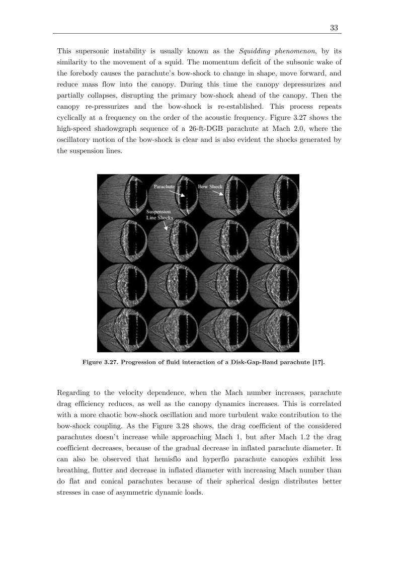
This supersonic instability is usually known as the Squidding phenomenon, by its
similarity to the movement of a squid. The momentum deficit of the subsonic wake of
the forebody causes the parachute’s bow-shock to change in shape, move forward, and
reduce mass flow into the canopy. During this time the canopy depressurizes and
partially collapses, disrupting the primary bow-shock ahead of the canopy. Then the
canopy re-pressurizes and the bow-shock is re-established. This process repeats
cyclically at a frequency on the order of the acoustic frequency. Figure 3.27 shows the
high-speed shadowgraph sequence of a 26-ft-DGB parachute at Mach 2.0, where the
oscillatory motion of the bow-shock is clear and is also evident the shocks generated by
the suspension lines.
Regarding to the velocity dependence, when the Mach number increases, parachute
drag efficiency reduces, as well as the canopy dynamics increases. This is correlated
with a more chaotic bow-shock oscillation and more turbulent wake contribution to the
bow-shock coupling. As the Figure 3.28 shows, the drag coefficient of the considered
parachutes doesn’t increase while approaching Mach 1, but after Mach 1.2 the drag
coefficient decreases, because of the gradual decrease in inflated parachute diameter. It
can also be observed that hemisflo and hyperflo parachute canopies exhibit less
breathing, flutter and decrease in inflated diameter with increasing Mach number than
do flat and conical parachutes because of their spherical design distributes better
stresses in case of asymmetric dynamic loads.
Figure 3.27. Progression of fluid interaction of a Disk-Gap-Band parachute [17].

34
The shape, scale and proximity of the parachute and bluff-body vehicle affect
parachute performance. The ratio of vehicle diameter to parachute nominal diameter
(𝑑/𝐷0) is a measure of the contribution of the wake to the fluid-structure interaction.
The non-dimensional trailing distance (𝑥/𝑑) is defined as the axial distance between
the parachute leading-edge and the vehicle maximum diameter. Knowing this, wind
tunnel tests [16] demonstrated that an increase in 𝑑/𝐷0 tends to reduce the flow field
unsteadiness and similarly, an increase in trailing distance reduces the coupling of the
wake to bow-shock and the drag coefficient is higher. Therefore, in the limit of 𝑥/𝑑 →
∞ or 𝑑/𝐷0 → 0, the effective vehicle diameter approaches zero, i.e. the flow field
approaches that of the parachute without an upstream wake contribution.
In general, the flow-dynamics is strongly associated with the parachute geometric
parameters and is dependent on the degree of coupling between the wake and
parachute bow-shock. Thereby, the selection of an appropriate trailing distance can
reduce coupling, but it must be traded with an orderly deployment process, parachute
inflation time, and multibody dynamics considerations.
Figure 3.28. Drag Coefficient of several parachutes as function of Mach number [16].

35
CHAPTER 4: Application. Parachute design
for the recovery of a rocket’s first-stage
In this section the concepts developed in the previous chapter will be applied to a real
case of recovery of the first stage of a rocket, which as we saw in the first chapter, the
recovery and subsequent reuse of the components of a rocket has become a very
important aspect for future space transport systems. Thus, from the data compilation
of the mission of this real case we will be able to make a preliminary design of the
recovery system of the first stage of the rocket. Therefore, through performance and
system analysis we can choose which type of parachute to select for high-speed
deceleration and for final recovery. We will try to verify as much as possible the design
considered with the real design, but of course we must take into account that different
engineers may make different selections based on experiences with particular types of
parachutes.
4.1. Ares I-X: Overview and General data
The rocket selected to make the preliminary design of the recovery system is the Ares
I-X, since in it we find a recovery system based on parachutes in which we can apply
properly the concepts studied in the last chapter.
Ares-I is one of the first rockets of the next-generation space transportation systems
developed by NASA’s Constellation Program to deliver explorations beyond the low
Earth orbit. The first flight test of this Program, known as Ares I-X, was on October
2009 and provided NASA an opportunity to test and prove hardware, models, facilities
and ground operations associated with the Ares I launch vehicle. This flight test
vehicle was built to demonstrate the flight control system performance during ascent
and gathering information to help engineers to find a final design of the Ares-I vehicle.
The Ares I-X vehicle consisted of two main parts: a functional five-segment solid rocket
booster stage (First Stage, FS) and an Upper Stage (US).
The US consists of eleven segments: two interstage segments, two ballast segments, five
“common” segments, and the spacecraft adapter and service module. These together
account more than 30 meters of the total 99.6-meter vehicle height and almost 205,000
kilograms of the Ares I-X vehicle’s lift-off weight.
The FS is approximately 53 meters in length and is responsible for lifting the entire
Ares I off the ground toward Earth orbit. It comprises a five-segment solid rocket
booster. It has an aluminium aft skirt, which provides structural support for the vehicle
and a forward skirt extension that contains the avionics system and the parachute
recovery system. The frustum which is made of a composite material, interfaces with
the US and contains the aeroshell, which houses the pilot and drogue parachutes.

36
Figure 4.1 shows a scheme of the different important parts of the Ares I and Table 4.1
lists some information gathered about the mass properties and dimensions of Ares I:
ARES I-X GENERAL
Length 99,6 m
Diameter 5,5 m
Total Mass 803,5 tons
4.1.1. Flight Performance
At launch, the thrust produced by the engine is greater than the weight of the rocket
and the net force accelerates the rocket away from the pad. Leaving the pad, the rocket
begins a powered vertical ascent. The vehicle accelerates because of the high thrust and
decreasing weight and rather quickly moves out of the thick atmosphere near the
surface of the Earth. Although the rocket is traveling supersonically, the drag on the
vehicle is small because of the shape of the rocket and the lower air density at higher
altitude. As the rocket ascends, it also begins to pitch over and its flight path becomes
more inclined to the vertical.
After approximately two minutes into the ascent, the propellants burn off and the first
stage becomes a near-empty tankage and must be discarded to allow the rest of the
vehicle to continue its ascent trajectory. This process is called staging. The discarded
first stage continues on a ballistic flight back to the Earth. At this point we will focus
only on the trajectory of the first stage and it will be described in more detail [18].
ARES I-X General
Length 99.6 m
Diameter 5.5 m
Total M ass 803.5 tons
Upper Stage
Length 46.9 m
Diameter 5.5 m
Total M ass 220 tons
First Stage
Length 52.7 m
Diameter 3.7 m
Total M ass 583.5 tons
Empty M ass 126.2 tons
Table 4.1. Dimensions and M ass properties [18].
Figure 4.1. Ares I Elements [18].

37
Staging of the Ares I-X occur near Mach 4.6 at an altitude of 40,000 meters and a
dynamic pressure of 4.8 kPa. The Ares I-X separation plane is located at the base of
the frustum. At staging, eight Booster Deceleration Motors (BDMs), located on the FS
aft skirt, are ignited to reduce the velocity of the FS relative to the US. During this
time the FS moved primarily in an axial direction relative to the US. Three seconds
after staging, four Booster Tumble Motors (BTMs), also located on the aft skirt of the
FS, are ignited to induce a tumbling motion predominantly about the negative yaw-axis
in order to increase drag and reduce re-entry dynamic pressure. Both the BDMs and
BTMs have short (~3 seconds) burn times, and the FS subsequently descend,
unpowered and uncontrolled, until parachute deployment.
For the first 15-20 seconds after staging, the FS is in the wake of the US and thus is
subjected to aerodynamic interference effects. The FS reach an apogee altitude of
approximately 46,000 meters nearly 38 seconds after staging and 90 seconds later (130
seconds after staging) it reach a maximum dynamic pressure (max-q) of 42 kPa at an
altitude of 16,600 meters.
Once the FS descend to an altitude of approximately 4,500 meters the FS nose cap is
jettisoned, releasing a pilot chute that deploys the drogue parachute with 20 meters of
nominal diameter. The drogue parachute reaches full inflation, decelerating the FS and
orienting it into a tail-first attitude. Then, the main parachutes (45-m nominal
diameter each one) are deployed as the forward skirt extension (FSE) is separated [18].
Figure 4.2 shows a sketch of the recovery trajectory of the first stage:
[………………………………….]
Figure 4.2. Recovery Trajectory of the first stage [19].
13. FS Water
Impact
12. Descent in
Equilibrium 11. Main Chutes
Full Disreef
1. Separation
from US
2. Tumble
Motor Fire
3. Apogee 4. Reentry
max Q
5. Nose Cap
Jettision
6. Pilot Chute
Deploy 7. Drogue
Chute
Deploy Drogue
Chute
Partial
Disreef
8. Drogue
Chute Full
Disreef
9. Fwd Skirt
Extension
Separation
10. Main Chutes
Deploy
14. FS Water
Impact
Attenuation

38
FIRST STAGE RECOVERY Time
(s)
Altitude
(m)
Velocity
(m/s)
Dynamic Pressure
(Pa)
1. First Stage Separation. 0 40107.41 1487.42 4500.74
2. Tumble Motor Fire. 3 41483.28 1475.23 3638.9
3. Apogee. 38 46664.88 1368.55 1580.05
4. Reentry Max q. 128 16672.56 710.18 42134.62
5. Nose Cap Jettision. 191 4660.392 160.02 9576.05
6. Pilot Chute Deploy. 192 4553.712 160.02 9671.81
7. Drogue Chute Deploy. 194 4206.24 157.89 9767.57
8. Drogue Chute Full Disreef. 206 2560.32 118.87 6511.71
9. Fwd Skirt Extension Separation. 216 1371.6 103.63 5601.99
10. Main Chutes Deploy. 218 1143 117.35 7325.68
11. Main Chutes Full Disreef. 231 347.472 31.09 574.56
12. Descent in Equilibrium. 236 228.6 21.64 335.16
13. FS Water Impact. 245 0 21.64 335.16
14. FS Water Impact Attenuation. 306 0 12.19 95.76
Table 4.2. Events based on predicted nominal performance, unless otherwise noted [19].
From Table 4.2 it can be represented the following graphs that show the characteristics
on the behaviour of the Recovery System of Ares I-X’s first stage.
0
5000
10000
15000
20000
25000
30000
35000
40000
45000
50000
0200400600800100012001400
Altitude (
m)
Velocity (m/s)
Altitude vs Velocity
Figure 4.3. Altitude vs Velocity curve of Ares I-X performance data from Table 4.2.

39
0
200
400
600
800
1000
1200
1400
0 50 100 150 200 250 300
Velo
city (
m/s)
Time (s)
Velocity vs Time
Figure 4.5. Velocity vs Time curve of Ares I-X performance data from Table 4.2.
0
5000
10000
15000
20000
25000
30000
35000
40000
45000
0 50 100 150 200 250 300
Dynam
ic P
ress
ure
(P
a)
Time (s)
Dynamic Pressure vs Time
Figure 4.4. Dynamic Pressure vs Time curve of Ares I-X performance data from Table 4.2.

40
If an increase of Figure 4.3 is made, we can observe in greater detail the behaviour of
the first stage of the rocket when the parachute recovery system is activated.
We can distinguish mainly three different phases according to this graph.
First, a rapid descent is made to an altitude of about 1400 meters. In this phase is
precisely where the pilot chute followed by the drogue chute deploys. The latter is
capable of decelerating the vehicle to about 35% in less than 25 seconds.
Next, a sudden increase in speed is observed due to the transition between the
separation of the drogue chute and the deployment of the main parachutes. As
expected in this transition there is no decelerator element and therefore the speed
increases to 13% in a period of 2 seconds.
The second phase, in which the parachutes are reefed, a lower descent is observed, since
the reefed parachutes offer more drag than the drogue chute, and consequently the rate
of descent is smaller. Thus it is possible to reduce the speed more than 80% with
respect to the speed before the deployment of the parachutes.
Finally, in a third phase, it is observed that the speed remains constant with the
altitude. This is because the main parachutes are completely disreef and reach a state
of equilibrium in the descent.
0
500
1000
1500
2000
2500
3000
3500
4000
4500
5000
020406080100120140160
Altitude (
m)
Velocity (m/s)
Altitude vs Velocity
Figure 4.6. Enlargement of Altitude vs Velocity curve of Ares I-X performance.
41
4.2. Parachute Recovery System Design
In this section, a preliminary design will be made of the parachute system described in
the previous section, used for the recovery of the first stage of Ares I-X rocket. For this,
the design concepts described in Chapter 3 will be applied, with which we will be able
to obtain certain characteristic values of the parachute system and its performance.
Some of these values can be compared with the values of the real case and therefore we
can verify the degree of adequacy of these procedures as a tool to obtain a suitable
preliminary design. On the other hand, in those cases where veridical information is not
available in the specific case, we will simply try to apply the necessary procedures to
obtain the values that characterize the parachute and based on the experience of other
designs, we will discuss the validity of the results obtained.
4.2.1. M ain Parachute System Design
a) Nominal Diameter:
The main objective of the main parachute system is to decelerate the vehicle in its last
descent phase, period in which the load is already stabilized at a low altitude and a
relatively slower speed.
First, to try to approximate as much as possible the design calculations with the real
main parachute system, we will select a cluster of three Ringslot parachutes. Anyway
this choice can be justified.
On the one hand, the decision to use a parachute cluster instead of a single one is
mainly due to the safety they offer, since it is less probably that a catastrophic failure
could occur. Besides this, the cluster reduces the inflation time of the parachute and its
manufacture is much simpler.
On the other hand, among the possible types of parachute shown in appendix A, the
Ringslot parachute proves to be one of the most suitable choices under these operating
conditions. Experience has shown that this type of parachute worked successfully as a
final recovery parachute and also because of its lighter weight, good drag coefficient,
slower inflation rate (thus lower opening-shock load), and improved stability compared
to other canopies.
The size of the cluster is determined by calculating the total effective drag area
required. For this, it is necessary to select the required rate of descent, when the main
parachutes are full opened and thus in equilibrium descent. In this application, the
selected rate of descent must be 21.7 m/s at an altitude of 230 m (see Table 4.2).
𝑚𝐹𝑆 = 126.2 𝑡𝑜𝑛𝑠 = 126200 𝑘𝑔 (Table 4.1) ; 𝑣1 = 𝑣(𝑧 = 230𝑚) = 21.7 𝑚/𝑠 (4.1)

42
Therefore, in equilibrium descent, the equilibrium dynamic pressure must be the same
at both 230 m altitude and sea level. Knowing this, it can be obtained an expression of
the rate of descent as a function of altitude:
𝑞𝑒 =1
2𝜌(𝑧)𝑣2 ; 𝜌(𝑧) = 𝜌0(1 − 22.57 · 10
−6𝑧)4.256 ; 𝜌0 = 1.225 𝑘𝑔/𝑚3
(4.2)
1
2𝜌(𝑧 = 230𝑚)𝑣1
2 =1
2𝜌0𝑣0
2 → 𝑣0 = 𝑣1√𝜌1𝜌0 ; 𝑧0 < 𝑧 < 𝑧1 (4.3)
Applying equation (4.3), the velocity of descent at sea level is 𝑣0 = 21.5 𝑚/𝑠, which is a
value very close to the value of the speed of descent acquired in the real case.
Considering that in equilibrium descent the total drag of the system is very nearly
equal to its weight, the required effective drag area can be obtained.
𝑊 = 𝐷 = (𝐶𝑑𝑆0) 𝑞𝑒 → (𝐶𝑑𝑆0) =𝑊
𝑞𝑒=2 𝑚𝐹𝑆 𝑔
𝜌(𝑧)𝑣2 ; 𝑧0 < 𝑧 < 𝑧1 (4.4)
In this case, the equilibrium dynamic pressure is 𝑞𝑒 = 282.102 𝑃𝑎, and the total drag
area is (𝐶𝑑𝑆0) = 4384.1 𝑚2, which is equivalent to an individual drag area for each
main parachute of (𝐶𝑑𝑆0)1,2,3 = 1461.4 𝑚2.
Once the drag area of each parachute is determined, the nominal surface can be
estimated and consequently the nominal diameter of each parachute of the cluster. At
this point it is necessary to make an assumption about the drag coefficient of the
parachute, since we don’t have a real value of it. Considering that a ringsail parachute
usually has a drag coefficient from 0.75 to 0.9 (see Appendix A), we can determine the
drag coefficient of each parachute representing a correlation between the nominal
diameter and the drag coefficient from data of different parachutes. These parachutes
are ringsail type, but built with different diameters [20].
y = -0,0002x2 + 0,0163x + 0,5118 R² = 0,9161
0,5
0,55
0,6
0,65
0,7
0,75
0,8
0,85
0,9
0,95
1
0 10 20 30 40 50 60
Dra
g C
oeffic
ient, C
D
Nominal Diameter , D0 (m)
CD vs Nominal Diameter
Figure 4.7. Typical drag coefficient versus nominal diameter for different sizes of
ringsail parachutes [20].

43
According to the graph of Figure 4.7, a typical drag coefficient value for a parachute of
45 m in diameter is 0.84, but in a cluster of three parachutes there is a drag loss
(section 3.5.1). Nevertheless this drag loss can be attenuated by lengthening the
suspension lines (section 3.4.5). Figures 4.8 and 4.9, based on experimental data of
different parachute systems, can give an idea of the percentage of drag change.
Figure 4.8. Drag loss in Parachute Clusters [2].
Figure 4.9. Variation of Drag Coefficient with Suspension Line Ratio [2].

44
As can be seen the percentage of drag loss is less than 5% for a cluster of three
parachutes, and this drag loss can be almost recover with a ratio 𝑙𝑒/𝐷0 greater than
1.2. Therefore for this preliminary design, this issue doesn’t mean a serious problem
and can be obviated.
𝐶𝑑 = 0.84 → 𝑆0 =𝐶𝑑𝑆0𝐶𝑑
→ 𝐷0 = √4 𝑆0𝜋
(4.5)
Using these equations, for each canopy the nominal surface is 𝑆0 = 1739.1 𝑚2 and the
nominal diameter is 𝑫𝟎 = 𝟒𝟕. 𝟎𝟓 𝒎. Comparing the latter with the nominal diameter of
the parachutes used in the Ares’s first stage (Section 4.1.1), it can be deduced that it is
a practically identical value, and therefore the assumptions are correct.
b) Canopy Inflation Time:
In the final interval in which the main parachutes are deployed, two phases can be
differentiated: reefed and disreefed phase. For this reason it is necessary to determine
two inflation times for both reefed and disreefed stages.
Considering that during the reefed phase, the equation of motion is given by:
𝑚 �̈� = 𝑚𝑔 − 𝐷𝐹𝐵 −𝐷𝑃 (4.6)
Where 𝐷𝑃 is the drag generated by the parachute (𝜌
2(𝐶𝐷𝑆0)𝑅𝑣
2) and 𝐷𝐹𝐵 is the drag of
the forebody. The drag generated by the forebody can be calculated by considering the
flat plate analogy developed by Daniel P. Raymer [21]. This method consists of
calculating the drag generated by a flat plate, and correcting the result by a shape
factor (SF), which depends on the geometrical parameters that define the volume of the
body, and therefore takes into account that the boundary layer becomes thicker and
detaches compared to the flat plate.
𝐷𝐹𝐵 =𝜌
2𝑆𝑤𝑒𝑡 𝑣
2 𝐶𝑓 𝑆𝐹 (4.7)
Where:
- 𝜌 is the air density.
- 𝑆𝑤𝑒𝑡 is the wet surface of the forebody.
- 𝑣 is the velocity of the forebody.
- 𝐶𝑓 is the Friction Coefficient.
- 𝑆𝐹 is the Shape Factor.
According to Raymer, the Friction Coefficient 𝐶𝑓 can be calculated as a function of the
Reynolds number and the Mach number as follows:
𝐶𝑓 = 0.455 (log10 𝑅𝑒(𝐷0))−2.58(1 + 0.144 𝑀2)−0.65 (4.8)
45
In this case the velocity is a variable, therefore we can express the equation (4.8) as:
𝐶𝑓 = 0.455 (log10 (𝜌 𝑣 𝐷0𝜇
))−2.58
(1 + 0.144 (𝑣
𝑐𝑆)2
)
−0.65
(4.9)
Moreover, considering that the forebody has a cylindrical shape similar to an aircraft
fuselage, Raymer proposes that the Shape Factor can be calculated as follows:
𝑆𝐹 = (1 +60
𝑓3+
𝑓
400) (4.10)
Where 𝑓 is the ratio between the length of the forebody and its diameter, also known
as slenderness (𝑙𝐹𝐵/𝑑𝐹𝐵).
Therefore the force of resistance of the forebody in the instant in which the main
parachutes deploy (𝑣𝑅 = 117.35 𝑚/𝑠 and 𝑧𝑅 = 1143 𝑚 from Table 4.2) can be
calculated.
From Table 4.1 we can obtained the values of length and diameter of the forebody,
which allow to obtain the value of 𝑓 and consequently the value of 𝑆𝐹.
𝑓 =52.7
3.7= 14.24 → 𝑆𝐹 = (1 +
60
𝑓3+
𝑓
400) = 1.0564 (4.11)
In order to obtain the value of the Friction Coefficient, Reynolds and Mach numbers
must be calculated (see Chapter 2), and then equation (4.8) is applied.
𝑅𝑒 =𝜌 𝑣 𝐷0𝜇0
=1.096 · 117.35 · 47.05
17.894 · 10−6= 2.6595 · 107
𝑀 =𝑣
𝑐𝑆=
117.35
√𝑇0 · (1 − 22.57 · 10−6 · 1143)
= 0.349
(4.12)
𝐶𝑓 = 0.455 (log10 𝑅𝑒(𝐷0))−2.58(1 + 0.144 𝑀2)−0.65 = 0.002551 (4.13)
Then applying equation (4.7), the resulting Drag force of the forebody is:
𝐷𝐹𝐵 =𝜌
2𝜋 𝑙𝐹𝐵 𝑑𝐹𝐵 𝑣
2 𝐶𝑓 𝑆𝐹 = 12458.5 𝑁 (4.14)
Finally, obtaining the deceleration from the data of Table 4.2, the drag area of the
reefed parachute can be calculated rearranging equation (4.6):
�̈�~∆𝑣
∆𝑡=117.3 − 31.1
231 − 218= −6.63
𝑚
𝑠2 ; (𝐶𝐷𝑆0)𝑅 =
2 (𝑚(𝑔 − �̈�) − 𝐷𝐹𝐵)
𝜌𝑣2= 273.35 𝑚2 (4.15)
Therefore each parachute have an individual drag area of (𝐶𝐷𝑆0)𝑅1,2,3 = 91.12 𝑚2.

46
With this we can easily obtain the nominal area (𝑆0)𝑅 dividing by the drag coefficient
and thus we can obtain the nominal diameter (𝐷0)𝑅 of the reefed parachutes.
(𝑆0)𝑅 =(𝐶𝐷𝑆0)𝑅𝐶𝐷
= 108.435 𝑚2 → (𝐷0)𝑅 = √4 𝑆0𝜋
= 11.75 𝑚 (4.16)
Finally, applying the equation (3.10) the inflation time of both phases can be obtained.
In this case the constant n must be 𝑛1 = 8 and 𝑛2 = 2 for ringsail parachutes.
𝒕𝒇𝟏 = 𝟎. 𝟐𝟎 𝒔 ; 𝒕𝒇𝟐 = 𝟐. 𝟗𝟒 𝒔 (4.17)
These values can be considered acceptable, even though the real values are not
available, since if we observe the inflation sequence of other parachute examples, the
filling time values are similar. Figure 4.11 shows an example of a cluster of two 72.8 ft-
diameter conical, full-extended skirt parachutes with a 2200-kg payload.
Figure 4.11. Inflation Sequence profile for a 72.8 ft-diameter Parachtue [2].
0
200
400
600
800
1000
1200
1400
020406080100120
Altitude (
m)
Velocity (m/s)
Main Parachutes. Altitude vs Velocity
Figure 4.10. Altitude vs Velocity of the Main Parachutes.

47
c) Opening Forces:
To calculate parachute opening forces we can apply the Pflanz Method described in
section 3.4.2.d. First we must calculate the ballistic parameter to be able to determine
through the graph of Figure 3.16 the force reduction factor 𝑋1.
For the reefed parachutes we have the following data:
𝑚1 = 𝑚𝐹𝑆/3 = 42066.7 𝑘𝑔
(𝐶𝐷𝑆)𝑅 = 91.12 𝑚2
𝜌(𝑧𝑅) = 1.096 𝑘𝑔/𝑚3
𝑔 = 9.81 𝑚/𝑠2
𝑣𝑅 = 117.35 𝑚/𝑠𝑡𝑓1 = 0.20 𝑠 }
→ 𝐴𝑅 =2 𝑊1
(𝐶𝐷𝑆)𝑅 𝜌 𝑔 𝑣𝑅 𝑡𝑓1= 35.89 (4.18)
In the case of the disreefed parachute we have:
𝑚1 = 𝑚𝐹𝑆/3 = 42066.7 𝑘𝑔
(𝐶𝐷𝑆)𝐷 = 1461.4 𝑚2
𝜌(𝑧𝐷) = 1.185 𝑘𝑔/𝑚3
𝑔 = 9.81 𝑚/𝑠2
𝑣𝐷 = 31 𝑚/𝑠𝑡𝑓2 = 2.94 𝑠 }
→ 𝐴𝐷 =2 𝑊1
(𝐶𝐷𝑆)𝐷 𝜌 𝑔 𝑣𝐷 𝑡𝑓2= 0.533 (4.19)
Before continuing we can observe that the ballistic parameter in this case takes low and
different values because the canopy loading is relatively low (𝑊/(𝐶𝐷𝑆)𝑅 = 461.7 𝑘𝑔/𝑚2 and
𝑊/(𝐶𝐷𝑆)𝐷 = 28.8 𝑘𝑔/𝑚2 ). Therefore, as section 3.4.3 (Altitude effects) explains, before we
get the values of the opening forces we can predict that they will decrease in descend
because of the strong velocity decrease (finite mass conditions).
Figure 4.12. Opening-Force reduction factor versus Ballistic Parameter.

48
From Figure 3.17 we obtain that the force reduction factors are (𝑋1)𝑅 = 1 for the reefed
phase and (𝑋1)𝐷 = 0.4 for the disreefed phase. Finally according to Appendix A, for
this preliminary design the opening-force coefficient can be considered 𝐶𝑋 = 1.05. With
this the opening forces for each parachute can be obtained using equation (3.11).
(𝐹𝑋)𝑅𝑒𝑒𝑓𝑒𝑑 = (𝐶𝐷𝑆)𝑅 · 𝑞𝑅 · 𝐶𝑋 · (𝑋1)𝑅 = 722032 𝑁
(𝐹𝑋)𝐷𝑖𝑠𝑟𝑒𝑒𝑓𝑒𝑑 = (𝐶𝐷𝑆)𝐷 · 𝑞𝐷 · 𝐶𝑋 · (𝑋1)𝐷 = 349385 𝑁 (4.20)
These are the opening forces applied on one main parachute and as expected, the
opening force decreases almost half. These opening forces are one of the most important
aspects in the design of the parachute system, since from them it is possible to choose
the material that is able to withstand these forces. As we saw in section 3.4.3, an
opening of the parachutes at an altitude higher than expected could cause serious
damage to the parachute system, as it would experience forces greater than expected at
a lower altitude.
Indeed, investigating some of the tests made with the Ares I-X rocket, this issue was a
big problem in one of the tests of recovery of the first stage of the Ares I. It can be
observed in the video captures of Figure 4.13 that there have been indeed problems in
this matter. In particular Figure 4.13 shows that one of the parachutes fails during its
opening, although the rest remain and avoid a catastrophic failure.
6.
1. 2. 3.
4. 5.
Figure 4.13. Sequence of images of the deployment of the main parachutes of the first stage
of the Ares I-X [22].

49
d) Weight Estimation:
Since we don’t have most of the measurements of the components of the parachute,
except the diameter of the main parachutes, it is not possible to make an estimation of
the complete parachute system weight, however it is possible to calculate a value of the
canopy weight using the K. E. French method (Section 3.3.6.d).
First, knowing that 𝑁𝑆𝐿𝑃𝑠 = 𝐹𝑋, we can rewrite the equation (3.4) as following:
𝑊𝑐𝑎𝑛𝑜𝑝𝑦 = (1.9 · 10−5(𝐹𝑋𝐷0)
0.96) (4.21)
Therefore, the obtained value of the canopy weight is 𝑾𝒄𝒂𝒏𝒐𝒑𝒚 = 𝟏𝟔𝟎. 𝟕𝟏 𝒌𝒈 and
consequently the three canopies would weigh 𝑾𝟑𝒄𝒂𝒏𝒐𝒑𝒊𝒆𝒔 = 𝟓𝟖𝟐. 𝟏𝟐 𝒌𝒈.
To contrast this result, we can make a similar procedure from data collected from other
ringsail canopies made of nylon as the main material. [20]. If these data are represented
in a graph, we obtain a curve with an exponential tendency, from which we can deduce
that the canopy weight is:
𝑊𝑐𝑎𝑛𝑜𝑝𝑦 = 0.0598 𝐷02.046 → 𝑾𝒄𝒂𝒏𝒐𝒑𝒚 = 𝟏𝟓𝟖. 𝟑𝟖 𝒌𝒈 → 𝑾𝟑𝒄𝒂𝒏𝒑𝒔 = 𝟒𝟕𝟓. 𝟏𝟓 𝒌𝒈 (4.22)
These two values of canopy weight obtained present a difference of about 2 kg for each
canopy, which allows us to deduce that it is quite probable that the real canopy has a
weight around 160 kg.
y = 0,0598x2,0465 R² = 0,9964
0
50
100
150
200
250
300
0 10 20 30 40 50 60
Canopy W
eig
ht
(kg)
Nominal Diameter, Do (m)
Canopy weight Vs Nominal diameter
Figure 4.14. Canopy Weight versus Nominal Diameter for different sizes Ringsail
Parachutes [20].
50
4.2.2. Drogue Chute Design
a) Nominal Diameter:
The following operational requirements govern the design of the drogue chute:
- The drogue chute must have a reliable operation in the velocity range from
157.9 m/s at 4206 meters (Point 7, Table 4.2).
- The drogue chute must be able to decelerate the forebody to the permissible
opening speed of the main parachute assemblies, which is 103.6 m/s at an
altitude of 1371 meters (Point 9, Table 4.2).
Evaluating the possible drogue chute candidates from Appendix A, the conical ribbon
parachute meets all requirements and has a higher drag coefficient than the equally
suited hemisflo parachute. The drag coefficient determines the parachute size and its
associated weight and volume.
As we can see in Figure 4.6, the behaviour of the drogue chute is similar to that of the
main reefed parachutes. Therefore the diameter of the drogue chute can be determined
with the same procedure used to determine the diameter of the reefed parachutes.
Applying equation (4.14), the drag of the forebody, when the descent velocity is
𝑣 = 157.9 𝑚/𝑠, is:
𝐷𝐹𝐵 =𝜌
2𝜋 𝑙𝐹𝐵 𝑑𝐹𝐵 𝑣
2 𝐶𝑓 𝑆𝐹 = 16352.8 𝑁 (4.23)
Obtaining the deceleration from the data of Table 4.2, the drag area of the drogue
chute can be calculated using equation (4.15):
�̈�~∆𝑣
∆𝑡=103.6 − 157.9
216 − 194= −2.467 𝑚/𝑠2 (4.24)
(𝐶𝐷𝑆0)𝐷𝐶 =(2 (𝑚(�̈� − 𝑔) + 𝐷𝐹𝐵)
𝜌𝑣2= 153.5 𝑚2 (4.25)
Therefore, assuming that the conical ribbon parachute has a drag coefficient 𝐶𝐷 = 0.5,
we can obtain the nominal area and consequently the nominal diameter:
(𝑆0)𝐷𝐶 =(𝐶𝐷𝑆0)𝐷𝐶
𝐶𝐷 = 307.039 𝑚2 → (𝐷0)𝐷𝐶 = √
4 𝑆0𝜋
= 𝟏𝟗. 𝟕𝟕 𝒎 (4.26)
Comparing the value of this nominal diameter with that one of the drogue chute used
in the Ares’s first stage (𝐷0𝐷𝐶 = 20 𝑚, Section 4.1.1), it can be deduced that it is a
practically identical value, and therefore the assumptions are correct.

51
Figure 4.15. Opening-Force reduction factor versus Ballistic Parameter.
b) Canopy Inflation Time:
The inflation time can be calculated in this case using equation (3.6), specific for the
ribbon parachute.
𝑡𝑓𝐷𝐶 =8 · 𝐷0𝐷𝐶0.9 · 𝑣
→ 𝒕𝒇𝑫𝑪 = 𝟏. 𝟏𝟏 𝒔 (4.27)
c) Opening Forces:
In order to determine the Opening Force, we will apply again, just as the Section
4.2.1.c, the Pflanz method described in section 3.4.2.d.
Applying equation (3.12) the ballistic parameter is obtained:
𝑚1 = 126200 𝑘𝑔
(𝐶𝐷𝑆)𝐷𝐶 = 153.5 𝑚2
𝜌(4206) = 0.801 𝑘𝑔/𝑚3
𝑔 = 9.81 𝑚/𝑠2
𝑣𝐷𝐶 = 157.9 𝑚/𝑠𝑡𝑓1 = 1.11 𝑠 }
→ 𝐴𝑅 =2 𝑚1
(𝐶𝐷𝑆)𝐷𝐶 𝜌 𝑣𝐷𝐶 𝑡𝑓1= 1.194 (4.28)
From Figure 4.15 we obtain that the force reduction factor is (𝑋1)𝐷𝐶 = 0.5.
52
Finally according to Appendix A, the opening-force coefficient for the conical ribbon
parachute is 𝐶𝑋 = 1.05. With this the opening force can be obtained using equation
(3.11).
(𝐹𝑋)𝐷𝑟𝑜𝑔𝑢𝑒𝐶ℎ𝑢𝑡𝑒 = (𝐶𝐷𝑆)𝐷𝐶 · 𝑞𝐷𝐶 · 𝐶𝑋 · (𝑋1)𝐷𝐶 = 𝟖𝟎𝟒𝟒𝟗𝟕 𝑵 (4.29)
d) Weight Estimation:
Again, as in the Section 4.2.1.d, we can only calculate the weight of the canopy by
applying the K. E. French method (Section 3.3.6.d).
𝑊𝐷𝐶𝑐𝑎𝑛𝑜𝑝𝑦 = (1.9 · 10−5(𝐹𝑋𝐷𝐶𝐷0)
0.96) → 𝑊𝐷𝐶𝑐𝑎𝑛𝑜𝑝𝑦 = 𝟏𝟓𝟓. 𝟕 𝒌𝒈 (4.30)

53
CHAPTER 5: Impact Attenuation System .
General Design Considerations
5.1. Landing Analysis
The rate of descent, the allowable impact deceleration, the type of vehicle, or the
required deceleration stroke (or distance) are factors that determine need for impact
attenuation.
This required deceleration distance (stroke) can be defined as follows [2]:
𝑠 =𝑣12 − 𝑣2
2
2𝑔(𝑛 − 1) (5.1)
Where:
- 𝑠 is the required deceleration stroke (distance).
- 𝑣1 is the rate of descent at start of deceleration.
- 𝑣2 is the rate of descent at impact.
- 𝑔 is the acceleration of gravity.
- 𝑛 is the allowable impact deceleration factor in multiples of 𝑔.
Figure 5.1 shows the required deceleration stroke for any kind of vehicle as a function
of the rate of descent, 𝑣1, and the allowable impact deceleration, 𝑛, using the
assumption that the velocity at impact, 𝑣2, is zero. As it can be seen, the selection of
the impact attenuator best suited for the operation is mainly based on the required
deceleration stroke and the allowable impact deceleration. Because of this we can
differentiate three primarily types of impacts attenuators with different application
ranges: Crushable and frangible attenuators are suitable for low required deceleration
strokes and have a high impact deceleration; Inflatable airbags are best suited for
higher deceleration strokes than the crushable attenuators and also permit a low impact
deceleration; and Retrorockets are used for longer deceleration strokes and are very
suitable for low impact deceleration.
Some examples of allowable impact deceleration factors based on measured data and
experience are listed in Table 5.1 [2].
Operation Impact deceleration, g
Military airdrop cargo 20 to 35
Target drones, unmanned vehicle structures 20 to 30
Telemetry equipment 20 to 25
Sensitive electronics equipment 5 to 10
Aircrew members 6 to 10
Astronauts after long duration space flights 3 to 5
Table 5.1. Allowable Impact Decelerations [2].
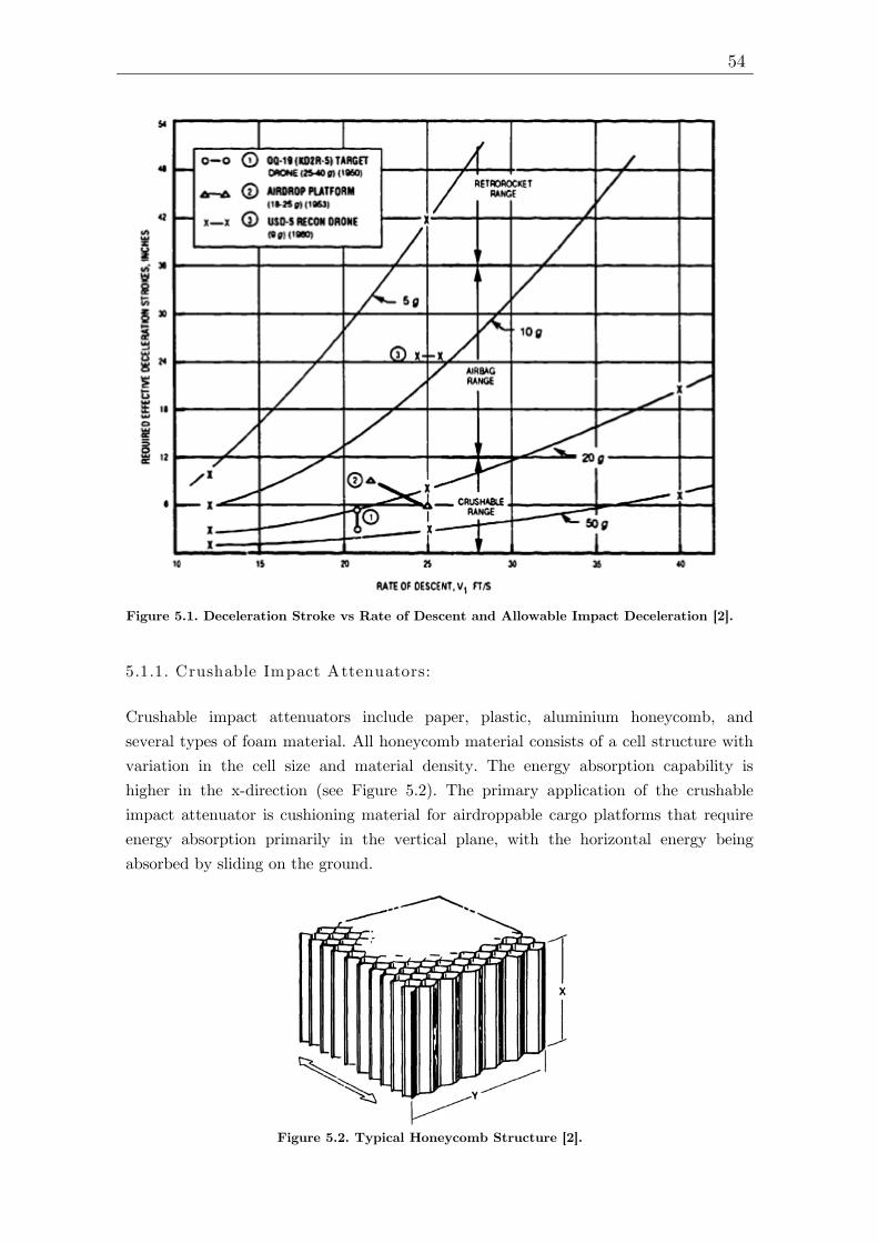
54
5.1.1. Crushable Impact Attenuators:
Crushable impact attenuators include paper, plastic, aluminium honeycomb, and
several types of foam material. All honeycomb material consists of a cell structure with
variation in the cell size and material density. The energy absorption capability is
higher in the x-direction (see Figure 5.2). The primary application of the crushable
impact attenuator is cushioning material for airdroppable cargo platforms that require
energy absorption primarily in the vertical plane, with the horizontal energy being
absorbed by sliding on the ground.
Figure 5.2. Typical Honeycomb Structure [2].
Figure 5.1. Deceleration Stroke vs Rate of Descent and Allowable Impact Deceleration [2].
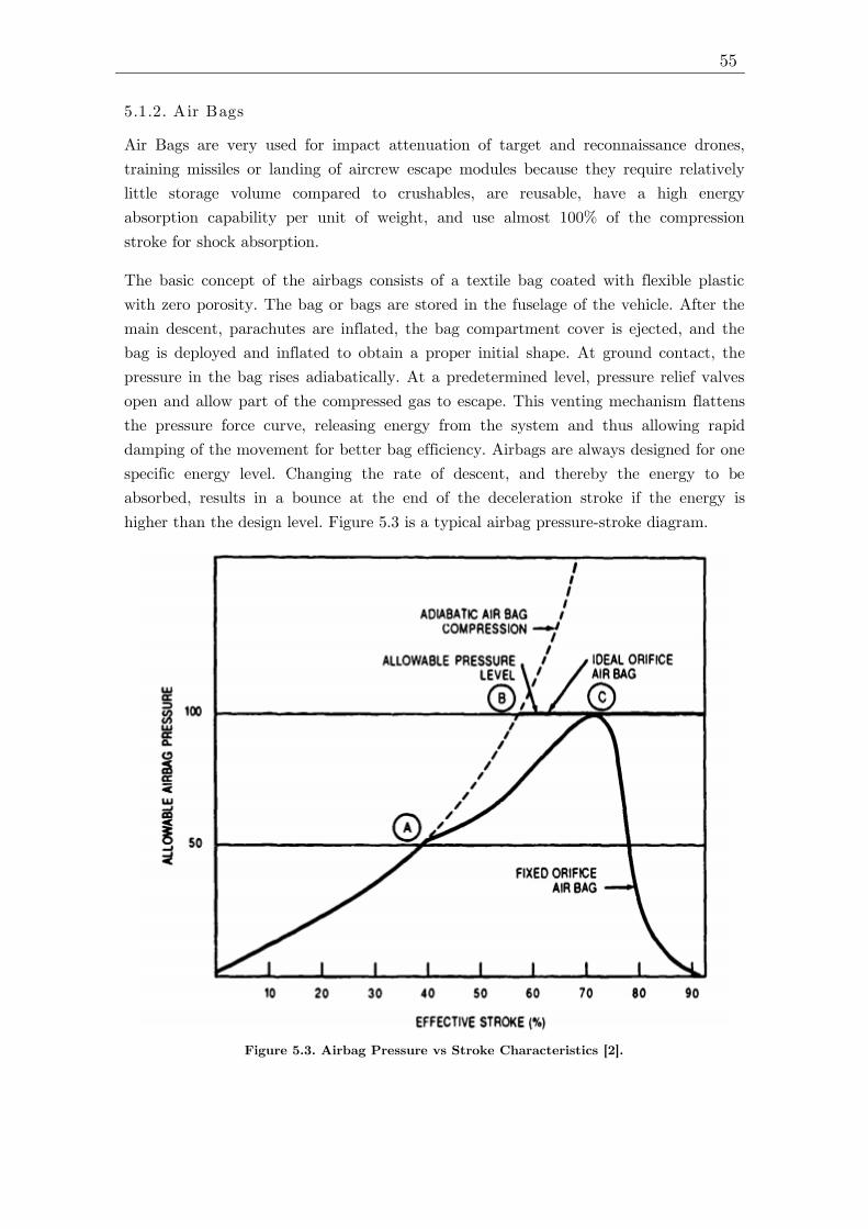
55
Figure 5.3. Airbag Pressure vs Stroke Characteristics [2].
5.1.2. Air Bags
Air Bags are very used for impact attenuation of target and reconnaissance drones,
training missiles or landing of aircrew escape modules because they require relatively
little storage volume compared to crushables, are reusable, have a high energy
absorption capability per unit of weight, and use almost 100% of the compression
stroke for shock absorption.
The basic concept of the airbags consists of a textile bag coated with flexible plastic
with zero porosity. The bag or bags are stored in the fuselage of the vehicle. After the
main descent, parachutes are inflated, the bag compartment cover is ejected, and the
bag is deployed and inflated to obtain a proper initial shape. At ground contact, the
pressure in the bag rises adiabatically. At a predetermined level, pressure relief valves
open and allow part of the compressed gas to escape. This venting mechanism flattens
the pressure force curve, releasing energy from the system and thus allowing rapid
damping of the movement for better bag efficiency. Airbags are always designed for one
specific energy level. Changing the rate of descent, and thereby the energy to be
absorbed, results in a bounce at the end of the deceleration stroke if the energy is
higher than the design level. Figure 5.3 is a typical airbag pressure-stroke diagram.

56
At ground contact, the bag starts to compress and the internal pressure increases until
at Point A, where the pressure relief valves open simultaneously, staggered or pressure
controlled. Then the pressure increase lessens until the allowable pressure level is
reached at Point C. Finally a pressure decay follows. The design of the pressure relief
valves contributes notably to the efficiency of the bag. Ideal orifices permit the bag
pressure to rise Point B and then remain constant until ground impact.
5.1.3. Retrorocket Landing Attenuation System
Retrorockets may be called long-stroke impact attenuators. Retrorockets are well suited
for loads and vehicles that have impact deceleration limits when landing in the 3- to 6-g
range that normally results in required deceleration strokes of more than 1 meter. The
main advantage of retrorockets is their high energy-weight ratio and their capability of
decelerating the vehicle before ground contact.
Retrorockets, like most other impact attenuators, are designed for one energy level but
this problem can be solved using a two-step rocket. The high thrust level is decreased
to a lowest energy level and then this low-energy deceleration stops the vehicle slightly
above the ground and gently lowers it for final landing.
5.2. Airbag Impact Dynamics M odelling
In this section the operation of the airbag system will be described in greater detail,
because it is the most appropriate impact attenuator for rocket’s stage recovery
applications. As its capabilities show in Section 5.1, airbag impact attenuation systems
are used for applications in which very strict allowable impact decelerations are not
required, as is the case for the recovery of the stage of a rocket. In addition they are
economically cheaper than the retrorockets and can have a second function of float for
those cases in which the landing takes place in the sea.
Fundamentally, airbags attenuate impact loads on objects through a series of energy
conversion processes. During landing, the kinetic energy of an impacting object is
transferred into the internal energy of the gas within the airbag. When predetermined
conditions are met, vents within the airbag open, releasing the gas into the open
environment and thereby removing this energy form the system. Although seemingly
simple, this process involves principles from several disciplines, including
thermodynamics, fluid mechanics and structural dynamics.
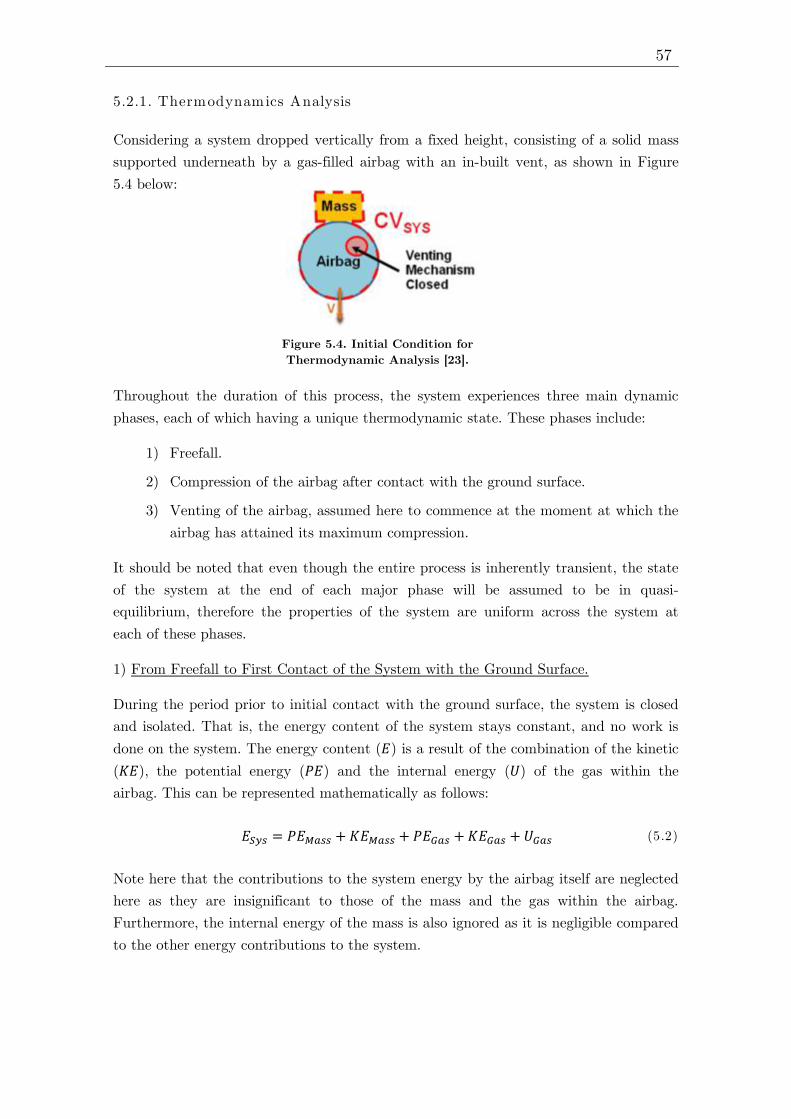
57
5.2.1. Thermodynamics Analysis
Considering a system dropped vertically from a fixed height, consisting of a solid mass
supported underneath by a gas-filled airbag with an in-built vent, as shown in Figure
5.4 below:
Throughout the duration of this process, the system experiences three main dynamic
phases, each of which having a unique thermodynamic state. These phases include:
1) Freefall.
2) Compression of the airbag after contact with the ground surface.
3) Venting of the airbag, assumed here to commence at the moment at which the
airbag has attained its maximum compression.
It should be noted that even though the entire process is inherently transient, the state
of the system at the end of each major phase will be assumed to be in quasi-
equilibrium, therefore the properties of the system are uniform across the system at
each of these phases.
1) From Freefall to First Contact of the System with the Ground Surface.
During the period prior to initial contact with the ground surface, the system is closed
and isolated. That is, the energy content of the system stays constant, and no work is
done on the system. The energy content (𝐸) is a result of the combination of the kinetic
(𝐾𝐸), the potential energy (𝑃𝐸) and the internal energy (𝑈) of the gas within the
airbag. This can be represented mathematically as follows:
𝐸𝑆𝑦𝑠 = 𝑃𝐸𝑀𝑎𝑠𝑠 + 𝐾𝐸𝑀𝑎𝑠𝑠 + 𝑃𝐸𝐺𝑎𝑠 +𝐾𝐸𝐺𝑎𝑠 +𝑈𝐺𝑎𝑠 (5.2)
Note here that the contributions to the system energy by the airbag itself are neglected
here as they are insignificant to those of the mass and the gas within the airbag.
Furthermore, the internal energy of the mass is also ignored as it is negligible compared
to the other energy contributions to the system.
Figure 5.4. Initial Condition for
Thermodynamic Analysis [23].
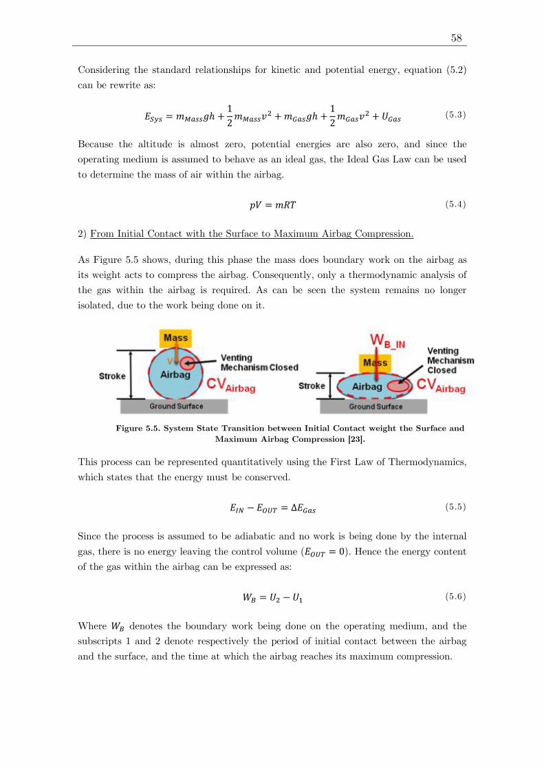
58
Considering the standard relationships for kinetic and potential energy, equation (5.2)
can be rewrite as:
𝐸𝑆𝑦𝑠 = 𝑚𝑀𝑎𝑠𝑠𝑔ℎ +1
2𝑚𝑀𝑎𝑠𝑠𝑣
2 +𝑚𝐺𝑎𝑠𝑔ℎ +1
2𝑚𝐺𝑎𝑠𝑣
2 + 𝑈𝐺𝑎𝑠 (5.3)
Because the altitude is almost zero, potential energies are also zero, and since the
operating medium is assumed to behave as an ideal gas, the Ideal Gas Law can be used
to determine the mass of air within the airbag.
𝑝𝑉 = 𝑚𝑅𝑇 (5.4)
2) From Initial Contact with the Surface to Maximum Airbag Compression.
As Figure 5.5 shows, during this phase the mass does boundary work on the airbag as
its weight acts to compress the airbag. Consequently, only a thermodynamic analysis of
the gas within the airbag is required. As can be seen the system remains no longer
isolated, due to the work being done on it.
This process can be represented quantitatively using the First Law of Thermodynamics,
which states that the energy must be conserved.
𝐸𝐼𝑁 − 𝐸𝑂𝑈𝑇 = ∆𝐸𝐺𝑎𝑠 (5.5)
Since the process is assumed to be adiabatic and no work is being done by the internal
gas, there is no energy leaving the control volume (𝐸𝑂𝑈𝑇 = 0). Hence the energy content
of the gas within the airbag can be expressed as:
𝑊𝐵 = 𝑈2 − 𝑈1 (5.6)
Where 𝑊𝐵 denotes the boundary work being done on the operating medium, and the
subscripts 1 and 2 denote respectively the period of initial contact between the airbag
and the surface, and the time at which the airbag reaches its maximum compression.
Figure 5.5. System State Transition between Initial Contact weight the Surface and
Maximum Airbag Compression [23].

59
The energy content of the system at this latter period can be observed by simply
rearranging equation (5.6).
𝑈2 = 𝑈1 −𝑊𝐵 (5.7)
In effect, equation (5.7) states that during the compression phase of the airbag, the
kinetic energy of the mass is being transferred into the internal energy of the gas via
the means of boundary work. The amount of kinetic energy transferred is equal to the
magnitude of the boundary work, which is defined as the integral of the system
pressure (𝑃) over its changing volume (𝑉).
𝑊𝐵 = ∫ 𝑃 𝑑𝑉2
1
(5.8)
A dependence on pressure and volume implies that boundary work, and hence the
efficiency of the energy transfer between the mass and the gas, is directly related to the
change in the geometry of the airbag as it compresses.
Assuming that the energy transfer process is completely efficient, the boundary work at
state 2 is equal to the kinetic energy of the mass and the gas at state 1.
𝑈2 = 𝑈1 − (𝐾𝐸𝑀𝑎𝑠𝑠 + 𝐾𝐸𝑔𝑎𝑠) (5.9)
3) From Airbag Venting to Rest.
The vents built into the airbag are opened immediately after it has reached its
maximum compression. At this point, the system becomes one which is open, as mass is
allowed to cross the boundary of the control volume.
To simplify the analysis, it will be assumed that boundary work is no longer being done
on the operating medium during this phase. As a consequence, 𝐸𝐼𝑁 = 0, and the energy
content of the system by the time it comes to rest can be represented by:
−𝑚𝑂𝑈𝑇(ℎ𝑂𝑈𝑇 + 𝑘𝑒𝑂𝑈𝑇) = 𝑈3 − 𝑈2 (5.10)
Figure 5.6. System during the Venting Phase [23].

60
Where ℎ𝑂𝑈𝑇 denotes the specific enthalpy, 𝑘𝑒𝑂𝑈𝑇 denotes the specific kinetic energy,
and the subscript 3 denotes the state of the system being at rest. Again, the energy
content of the system after this process can be expressed by rearranging equation (5.10)
as follows:
𝑈3 = 𝑈2 −𝑚𝑂𝑈𝑇(ℎ𝑂𝑈𝑇 + 𝑘𝑒𝑂𝑈𝑇) (5.11)
It can be seen that the final energy of the content of the system is equal to its energy
prior to venting, minus the energy removed by the kinetic energy and enthalpy of the
vented gas.
Ideally, this system would have zero energy at the end of the venting stage, signifying a
complete attenuation of the impact energy. To obtain an estimate for the proportion of
gas required to be vented to achieve this, 𝑈3 will be set to zero and equation (5.11) will
be solved for 𝑚𝑂𝑈𝑇.
𝑚𝑂𝑈𝑇 =𝑈2
ℎ𝑂𝑈𝑇 + 𝑘𝑒𝑂𝑈𝑇 (5.12)
5.2.2. System Dynamics Equation
From a fluid mechanics perspective, the change in airbag geometry is calculated based
on the position of the supported mass. This is then used to obtain the pressure, volume
and mass of the operating medium, which is in turn used to determine the conditions
for venting of the airbag.
Figure 5.7. Single Airbag Impact Model
Initial Condition [23].
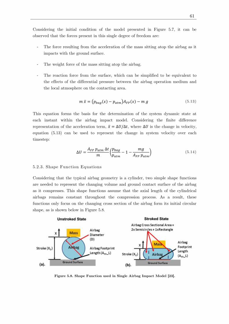
61
Considering the initial condition of the model presented in Figure 5.7, it can be
observed that the forces present in this single degree of freedom are:
- The force resulting from the acceleration of the mass sitting atop the airbag as it
impacts with the ground surface.
- The weight force of the mass sitting atop the airbag.
- The reaction force from the surface, which can be simplified to be equivalent to
the effects of the differential pressure between the airbag operation medium and
the local atmosphere on the contacting area.
𝑚 �̈� = (𝑝𝑏𝑎𝑔(𝑥) − 𝑝𝑎𝑡𝑚)𝐴𝐹𝑃(𝑥) − 𝑚 𝑔 (5.13)
This equation forms the basis for the determination of the system dynamic state at
each instant within the airbag impact model. Considering the finite difference
representation of the acceleration term, �̈� = ∆𝑈/∆𝑡, where ∆𝑈 is the change in velocity,
equation (5.13) can be used to represent the change in system velocity over each
timestep:
∆𝑈 =𝐴𝐹𝑃 𝑝𝑎𝑡𝑚 ∆𝑡
𝑚(𝑝𝑏𝑎𝑔
𝑝𝑎𝑡𝑚− 1 −
𝑚𝑔
𝐴𝐹𝑃 𝑝𝑎𝑡𝑚) (5.14)
5.2.3. Shape Function Equations
Considering that the typical airbag geometry is a cylinder, two simple shape functions
are needed to represent the changing volume and ground contact surface of the airbag
as it compresses. This shape functions assume that the axial length of the cylindrical
airbags remains constant throughout the compression process. As a result, these
functions only focus on the changing cross section of the airbag form its initial circular
shape, as is shown below in Figure 5.8.
Figure 5.8. Shape Function used in Single Airbag Impact Model [23].

62
A condition is enforced such that the circumference of the airbag cross section remains
constant. This can be expressed as:
𝜋𝐷 = 𝜋𝑋𝐷 + 2𝐿𝐴𝐹𝑃 (5.15)
Rearranging equation (5.15) the airbag footprint length can be written as a function of
the airbag stroke:
𝐿𝐴𝐹𝑃 = 𝜋(𝐷 − 𝑋𝐷) (5.16)
The cross sectional area of the airbag in the stroked state can be determined using the
fact that it consists of a rectangle and two semi-circles:
𝐴𝑋−𝑠𝑒𝑐𝑡𝑖𝑜𝑛 = 𝜋𝑋𝐷2/4 + 𝑋𝐷𝐿𝐴𝐹𝑃 (5.17)
Since the axial length (𝐿) is assumed to remain constant throughout the compression
process, the airbag volume and contact surface can be obtained.
𝐴𝐹𝑃(𝑋𝐷) = 𝐿 · 𝐿𝐴𝐹𝑃(𝑋𝐷) = 𝐿 𝜋(𝐷 − 𝑋𝐷) (5.18)
𝑉(𝑋𝐷) = 𝐿 𝐴𝑋−𝑠𝑒𝑐𝑡𝑖𝑜𝑛 = 𝐿 𝑋𝐷 (𝜋𝑋𝐷4+ 𝐿𝐴𝐹𝑃) (5.19)
5.2.4. Gas Dynamics Equation
A simplifying assumption is made such that the operating medium within the airbag
acts as an ideal gas, and that the process is isentropic.
Therefore the Ideal Gas Law can be applied:
𝑝 𝑉 = 𝑤 𝑅𝐺𝑎𝑠𝑇 (5.20)
Where 𝑝 is the pressure, 𝑉 is the volume, 𝑤 is the equivalent mass of the gas, 𝑅𝐺𝑎𝑠 is
the specific gas constant, and 𝑇 is the operating temperature.
And it can be also considered the Isentropic Process Equation:
𝑇2𝑇1= (
𝑝2𝑝1)
𝛾−1𝛾= (
𝜌2𝜌1)𝛾−1
(5.21)

63
Figure 5.9. Definition of Upstream and Downstream Pressure
as used by the Single Airbag Impact Model [23].
5.2.5. Orifice Flow Equations
The flow of a gas can be modelled using the mass flow equation applied at the location
of the orifice:
𝑑𝑤
𝑑𝑡= 𝐶𝐷 𝐴𝑡ℎ 𝜌𝑡ℎ 𝑣𝑡ℎ (5.22)
Where the subscript th indicates the state at the orifice, 𝐶𝐷 is the discharge coefficient
(a factor representing inefficiencies in the flow stream), 𝐴𝑡ℎ is the orifice area during
the current timestep, and 𝑣𝑡ℎ is the flow velocity through the orifice. The mass flow
rate through the orifice can be represented in terms of only the pressure and
temperature of the gas using the following equations:
Density form of the Ideal Gas Law applied at the orifice:
𝜌𝑡ℎ =𝑝𝑡ℎ
𝑅𝐺𝑎𝑠𝑇𝑡ℎ (5.23)
The velocity to the gas:
𝑣𝑡ℎ = 𝑀𝑡ℎ 𝑐𝑡ℎ ; 𝑐𝑡ℎ = √𝛾𝑅𝐺𝑎𝑠𝑇𝑡ℎ (5.24)
Combining equations (5.23) and (5.24) into equation (5.22), the mass flow rate is:
𝑑𝑤
𝑑𝑡= 𝐶𝐷 𝐴𝑡ℎ 𝑝𝑡ℎ 𝑀𝑡ℎ √
𝛾
𝑅𝐺𝑎𝑠𝑇𝑡ℎ (5.25)
Since there is close to zero average flow of gas within the airbag, a standard nozzle flow
equation can be used to relate the flow velocity through the orifice, to the ratio of
pressure at the orifice and upstream from it.
𝑝𝑡ℎ𝑝𝑢
= (1 +(𝛾 − 1)𝑀𝑡ℎ
2
2)
𝛾𝛾−1
(5.26)
Where 𝑝𝑢 indicates the pressure upstream from the orifice, that is effectively the same
pressure as of that to the airbag, as shown in Figure 5.9.
64
With this, equation (5.26) can be rearranged:
𝑀𝑡ℎ = (2
𝛾 − 1((𝑝𝑡ℎ𝑝𝑢)
1−𝛾𝛾− 1))
12
(5.27)
Substituting this result into equation (5.25) yields:
𝑑𝑤
𝑑𝑡= 𝐶𝐷 𝐴𝑡ℎ 𝑝𝑡ℎ (
2
𝛾 − 1((𝑝𝑡ℎ𝑝𝑢)
1−𝛾𝛾− 1))
12
(𝛾
𝑅𝐺𝑎𝑠𝑇𝑡ℎ)
12 (5.28)
Assuming that the gas at the orifice experiences an isentropic process from the initial
system state to the current state, the initial pressure and temperature of the gas at the
orifice are the same as those of the gas within the airbag.
1
𝑇𝑡ℎ=1
𝑇𝑖(𝑝𝑖𝑝𝑡ℎ)
𝛾−1𝛾
(5.29)
Thus, substituting equation (5.29) into equation (5.28) results in:
𝑑𝑤
𝑑𝑡= 𝐶𝐷 𝐴𝑡ℎ 𝑝𝑡ℎ (
2
𝛾 − 1((𝑝𝑡ℎ𝑝𝑢)
1−𝛾𝛾− 1))
12
(𝛾
𝑅𝐺𝑎𝑠)
12(1
𝑇𝑖(𝑝𝑖𝑝𝑡ℎ)
𝛾−1𝛾)
12
(5.30)
Finally, manipulating this equation and considering that the upstream pressure is
equivalent to the airbag pressure (𝑝𝑢 = 𝑝𝑏𝑎𝑔) and orifice pressure is equal to the local,
downstream atmospheric pressure (𝑝𝑡ℎ = 𝑝𝑎𝑡𝑚) the final form of this orifice flow
equation can be expressed as:
𝑑𝑤
𝑑𝑡= 𝐶𝐷 𝐴𝑡ℎ 𝑝𝑎𝑡𝑚 (
𝛾
𝑅𝐺𝑎𝑠 𝑇𝑖)
12 (
2
𝛾 − 1((𝑝𝑎𝑡𝑚𝑝𝑏𝑎𝑔
)
1−𝛾𝛾
− 1) (𝑝𝑖𝑝𝑎𝑡𝑚
)
𝛾−1𝛾)
12
(5.31)
In this last equation it can be seen that the mass flow rate is a function of the ratio
between the airbag pressure and the local atmospheric pressure. Moreover, it is
important to note that this relationship is only valid for subsonic flows.
In the case that the flow through the orifice is sonic, 𝑀𝑡ℎ = 1, equation (5.26) reduces
to:
𝑝𝑡ℎ𝑝𝑢
= (𝛾 + 1
2)
𝛾1−𝛾
(5.32)

65
Figure 5.10. Data used to model the Discharge Coefficient within the Single Airbag
Impact Model [24].
Proceeding in the same way as in the subsonic case, the equation for sonic flow through
the airbag orifice is given as:
𝑑𝑤
𝑑𝑡= 𝐶𝐷 𝐴𝑡ℎ 𝑝𝑖 (
𝛾
𝑅𝐺𝑎𝑠 𝑇𝑖)
12 ((
2
𝛾 + 1)
𝛾+1𝛾−1
(𝑝𝑏𝑎𝑔
𝑝𝑖)
𝛾+1𝛾)
12
(5.33)
In this case it can be observed that the sonic orifice flow has a flow rate that remains
constant and unaffected by the fluctuations in the pressure downstream of the orifice.
To determine if the flow through the orifice is subsonic or sonic, the pressure ratio
across the orifice compared to that of the critical pressure ratio of the operating
medium. This critical pressure ratio is defined as the ratio at which the flow is
accelerated to a velocity equal to that of the local velocity of sound. Subsequently, this
can be obtained from equation (5.32) substituting the appropriate ratio of specific heats
for a given operating medium. For atmospheric air at room temperature, this specific
heat ratio is 1.4 and thereby the critical pressure ratio is:
𝑝𝑡ℎ𝑝𝑢
= (𝛾 + 1
2)
𝛾1−𝛾
= (1.4 + 1
2)
1.41−1.4
= 0.528 (5.34)
Therefore, if the pressure ratio across the orifice is less than 0.528, the flow through the
orifice is subsonic and equation (5.31) applies. However, if the pressure ratio across the
orifice is greater than 0.528, the sonic orifice flow is given by equation (5.33).
* Discharge Coefficient
The discharge coefficient refers to the losses due to frictional and viscous effects as the
gas flow through the orifice, which varies as function of the pressure ratio across the
orifice. To model this effect, data obtained from orifice flow experiments conducted by
Perry [24] was used to form an empirical relationship between pressure ratio and
discharge coefficient.
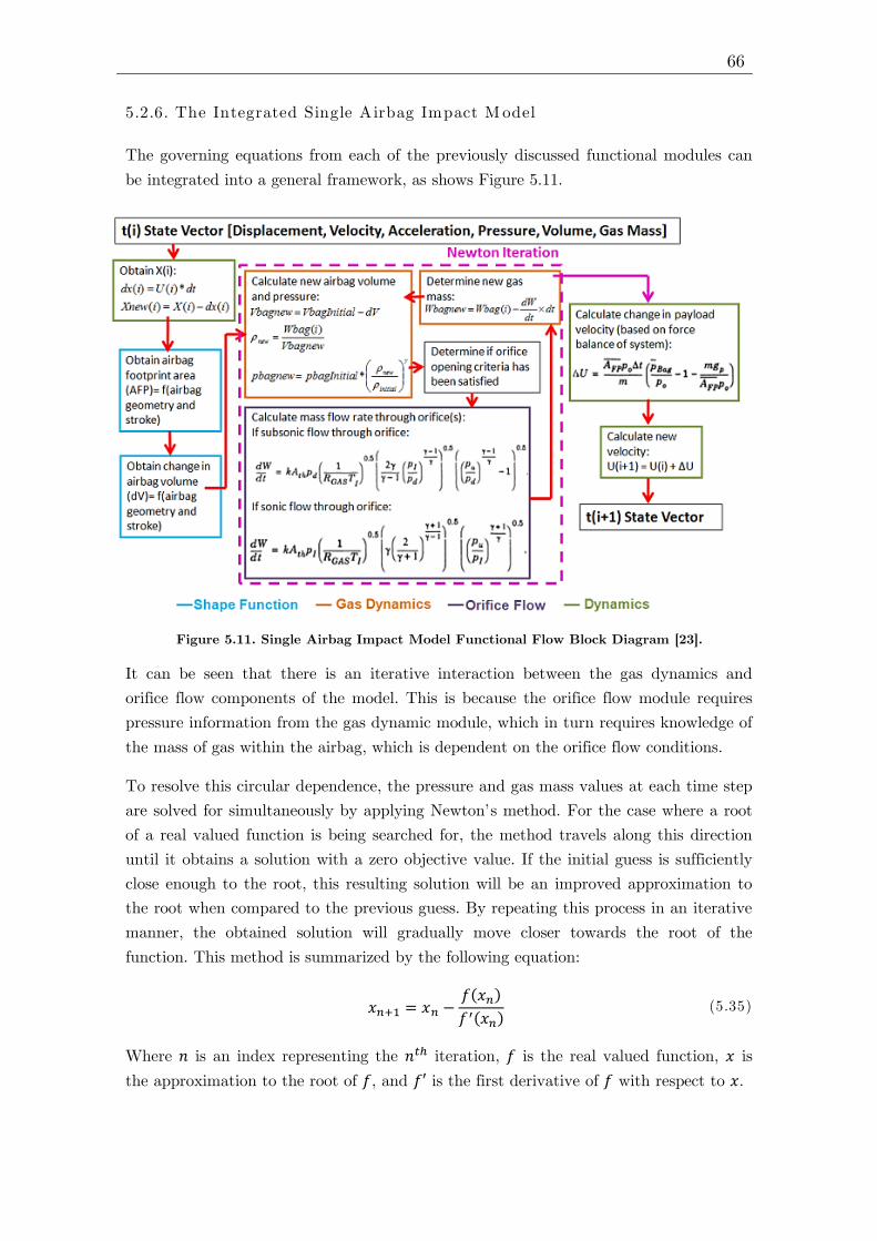
66
5.2.6. The Integrated Single Airbag Impact M odel
The governing equations from each of the previously discussed functional modules can
be integrated into a general framework, as shows Figure 5.11.
It can be seen that there is an iterative interaction between the gas dynamics and
orifice flow components of the model. This is because the orifice flow module requires
pressure information from the gas dynamic module, which in turn requires knowledge of
the mass of gas within the airbag, which is dependent on the orifice flow conditions.
To resolve this circular dependence, the pressure and gas mass values at each time step
are solved for simultaneously by applying Newton’s method. For the case where a root
of a real valued function is being searched for, the method travels along this direction
until it obtains a solution with a zero objective value. If the initial guess is sufficiently
close enough to the root, this resulting solution will be an improved approximation to
the root when compared to the previous guess. By repeating this process in an iterative
manner, the obtained solution will gradually move closer towards the root of the
function. This method is summarized by the following equation:
𝑥𝑛+1 = 𝑥𝑛 −𝑓(𝑥𝑛)
𝑓′(𝑥𝑛) (5.35)
Where 𝑛 is an index representing the 𝑛𝑡ℎ iteration, 𝑓 is the real valued function, 𝑥 is
the approximation to the root of 𝑓, and 𝑓′ is the first derivative of 𝑓 with respect to 𝑥.
Figure 5.11. Single Airbag Impact Model Functional Flow Block Diagram [23].

67
Therefore, a general Newton step for a function of pressure can be expressed as:
𝑝𝑡+∆𝑡,𝑛+1 = 𝑝𝑡+∆𝑡,𝑛 −𝑓(𝑝𝑡+∆𝑡,𝑛)
𝑓′(𝑝𝑡+∆𝑡,𝑛) (5.36)
Where 𝑝 is the airbag pressure, 𝑡 is a time coordinate and 𝑛 is an increment denoting
the iteration number. For the purposes of simplifying the notation used in this
derivation, let 𝑝𝑡+∆𝑡,𝑛 be denoted by 𝑝𝑛𝑒𝑤(𝑛) and 𝑝𝑡+∆𝑡,𝑛+1 by 𝑝𝑛𝑒𝑤(𝑛 + 1) .
Furthermore, let the pressure from the previous time step, that is 𝑝𝑡, be denoted by
𝑝𝑜𝑙𝑑. Thus, equation (5.36) becomes:
𝑝𝑛𝑒𝑤(𝑛 + 1) = 𝑝𝑛𝑒𝑤(𝑛) −𝑓(𝑝𝑛𝑒𝑤(𝑛))
𝑓′(𝑝𝑛𝑒𝑤(𝑛)) (5.37)
From this, explicit relationships for 𝑓(𝑝𝑛𝑒𝑤) and 𝑓′(𝑝𝑛𝑒𝑤), can be derived as follows:
𝒇(𝒑𝒏𝒆𝒘)
The relationship that describes the change in airbag pressure from one timestep to the
next is given by equation (5.21):
𝑝𝑛𝑒𝑤 = 𝑝𝑜𝑙𝑑 (𝜌𝑛𝑒𝑤𝜌𝑜𝑙𝑑
)𝛾
= 𝑝𝑜𝑙𝑑 (𝑤𝑛𝑒𝑤
𝜌𝑜𝑙𝑑𝑉𝑛𝑒𝑤)𝛾
= 𝑝𝑜𝑙𝑑 (𝑤𝑜𝑙𝑑 −
𝑑𝑤(𝑝𝑛𝑒𝑤)𝑑𝑡
𝑑𝑡
𝜌𝑜𝑙𝑑𝑉𝑛𝑒𝑤)
𝛾
(5.38)
Moreover, the mass flow rate component of this equation for subsonic flow (equation
(5.31)) can be expressed as:
𝑑𝑤
𝑑𝑡= 𝐶𝐷𝑝𝑛𝑒𝑤 𝐴𝑡ℎ 𝑝𝑎𝑡𝑚 (
𝛾
𝑅𝐺𝑎𝑠 𝑇𝑖)
12 (
2
𝛾 − 1((𝑝𝑎𝑡𝑚𝑝𝑛𝑒𝑤
)
1−𝛾𝛾− 1) (
𝑝𝑖𝑝𝑎𝑡𝑚
)
𝛾−1𝛾)
12
(5.39)
Substituting equation (5.39) into equation (5.38) yields:
𝑝𝑛𝑒𝑤 = 𝑝𝑜𝑙𝑑
(
1
𝜌𝑜𝑙𝑑𝑉𝑛𝑒𝑤
{
𝑤𝑜𝑙𝑑 − 𝑑𝑡 𝐶𝐷(𝑝𝑛𝑒𝑤) 𝐴𝑡ℎ 𝑝𝑎𝑡𝑚 (
𝛾
𝑅𝐺𝑎𝑠 𝑇𝑖)
12· →
→ · (2
𝛾 − 1((𝑝𝑎𝑡𝑚𝑝𝑛𝑒𝑤
)
1−𝛾𝛾− 1) · (
𝑝𝑖𝑝𝑎𝑡𝑚
)
𝛾−1𝛾)
12
}
)
𝛾
(5.40)
From this, a function in terms of 𝑝𝑛𝑒𝑤 can be determined by rearranging equation (5.40):
𝑓(𝑝𝑛𝑒𝑤) = 𝑝𝑜𝑙𝑑
(
1
𝜌𝑜𝑙𝑑𝑉𝑛𝑒𝑤
{
𝑤𝑜𝑙𝑑 − 𝑑𝑡 𝐶𝐷(𝑝𝑛𝑒𝑤) 𝐴𝑡ℎ 𝑝𝑎𝑡𝑚 (
𝛾
𝑅𝐺𝑎𝑠 𝑇𝑖)
1
2· →
→ · (2
𝛾 − 1((
𝑝𝑎𝑡𝑚
𝑝𝑛𝑒𝑤
)
1−𝛾
𝛾
− 1) · (𝑝𝑖
𝑝𝑎𝑡𝑚
)
𝛾−1
𝛾
)
12
}
)
𝛾
− 𝑝𝑛𝑒𝑤
(5.41)

68
𝒇′(𝒑𝒏𝒆𝒘)
Using the chain rule, equation (5.41) can be differentiated, with the following result:
𝑓′(𝑝𝑛𝑒𝑤) =𝑑𝑓(𝑝𝑛𝑒𝑤)
𝑑𝑝𝑛𝑒𝑤= 𝛾(𝑓(𝑝
𝑛𝑒𝑤) + 𝑝
𝑛𝑒𝑤)𝛾−1
· →
→ ·−𝑑𝑡𝐴𝑡ℎ𝑝𝑎𝑡𝑚𝜌𝑜𝑙𝑑𝑉𝑛𝑒𝑤
(𝛾
𝑅𝐺𝑎𝑠𝑇𝑖)
0.5
(2
𝛾 − 1(𝑝𝑖𝑝𝑎𝑡𝑚
)
𝛾−1𝛾)
0.5
· →
→ ·
(
𝐶𝐷( 𝑝𝑛𝑒𝑤) ((
𝑝𝑛𝑒𝑤𝑝𝑎𝑡𝑚
)
𝛾−1𝛾− 1)
0.5
+ →
→ +0.5 𝐶𝐷′ ( 𝑝𝑛𝑒𝑤) ((
𝑝𝑛𝑒𝑤𝑝𝑎𝑡𝑚
)
𝛾−1𝛾− 1)
−0.5
· (𝛾 − 1
𝛾) (𝑝𝑛𝑒𝑤𝑝𝑎𝑡𝑚
)−1𝛾
)
− 1
(5.43)
With this, equations (5.41) and (5.42) can be substituted into equation (5.37) and
computationally implemented into an iterative scheme to obtain the pressure and gas
solution over a given timestep.
69
CHAPTER 6: Application: A irbag design for the
recovery of a rocket’s first-stage
In this section we will obtain the proposal of a preliminary design for an Airbag based
on the characteristics and behaviour of the first stage of the Ares I-X rocket. It is a
completely invented approach, since the rocket does not actually have such an impact
attenuation system. To do this we will use the concepts described in Chapter 5 and try
to dimension the airbag system and its performance.
6.1. Airbag Sizing
Before beginning the design of the airbag, we must consider how the position of the
airbag should be to fulfil its impact attenuation function.
Firstly, according to the recovery performance of the FS described in Section 4.1.1, the
vehicle impacts with a completely vertical position at a speed of 21.64 m/s. The impact
in this vertical position implies that the lower end of the vehicle suffers the greatest
loads, i.e. most of the stresses are concentrated in the lower part of the vehicle and
therefore suffer more damage than the upper end. For this reason it would be necessary
to design a very robust attenuation system to absorb such loads.
It is physically more logical that the vehicle impacts the surface in a horizontal
position, because with this the impact stresses are spread uniformly throughout the
structure. In addition the airbag system in this case can be designed along the entire
length of the vehicle and as a secondary function can work as a flotation system to
prevent the sinking of the vehicle.
In short, the airbag design to be considered must attenuate the impact of the FS in
horizontal position instead of vertical position. For this we must also design a
mechanism that can change the vertical position of the FS to a horizontal position.
This mechanism can be another parachute system that is deployed at the lower end of
the vehicle. This mechanism involves reconsidering the recovery action of the first stage
in its final phase, i.e. once the main parachutes have been fully opened.
Therefore we must now consider that a second parachute system is deployed. To
achieve a horizontal position, this parachute system must be identical to the main
parachutes, i.e. a cluster of 3 parachutes of 45 meters in diameter and with the same
drag area (4384.1 m2).

70
With these two clusters of 3 parachutes, the speed of descent in equilibrium will be
much smaller than the previous one (21.64 m/s). This speed is difficult to determine
due to the oscillations that the vehicle can suffer until it stabilizes completely in
horizontal position. Therefore to continue with the design of the airbag, we will assume
that the parachute system descends in equilibrium from 200 meters and with a speed of
10 m/s.
6.2. Airbag performance
The first issue is to find the volume of air that the airbag needs to absorb all the
energy of the impact. The method used to solve this problem is based on the
thermodynamic analysis (section 5.2.1), with which we can study the energy state of
the system in each of the three phases of the impact and we can obtain the required
mass of air. For this we will consider certain assumptions based on other airbag impact
attenuation systems, such as the Orion CEV airbag system [25].
The initial data considered in this case are those mentioned in the previous section
(𝑣1 = 10 𝑚/𝑠 and 𝑧 = 0 𝑚). Regarding the Airbag, we will assume that the operating
medium is atmospheric air that is in normal conditions with an initial pressure of 130
kPa. Table 6.1 shows the assumed values for the thermodynamic analysis based on the
Orion CEV airbag system.
Figure 6.1. New Design of the Main Parachutes for the Final Descent.
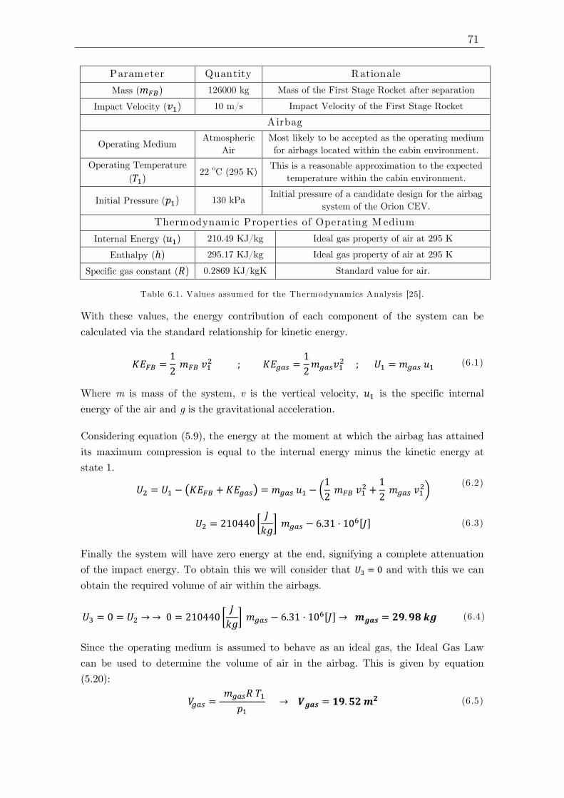
71
Parameter Quantity Rationale
Mass (𝑚𝐹𝐵) 126000 kg Mass of the First Stage Rocket after separation
Impact Velocity (𝑣1) 10 m/s Impact Velocity of the First Stage Rocket
Airbag
Operating Medium Atmospheric
Air
Most likely to be accepted as the operating medium
for airbags located within the cabin environment.
Operating Temperature
(𝑇1) 22
oC (295 K)
This is a reasonable approximation to the expected
temperature within the cabin environment.
Initial Pressure (𝑝1) 130 kPa Initial pressure of a candidate design for the airbag
system of the Orion CEV.
Thermodynamic Properties of Operating M edium
Internal Energy (𝑢1) 210.49 KJ/kg Ideal gas property of air at 295 K
Enthalpy (ℎ) 295.17 KJ/kg Ideal gas property of air at 295 K
Specific gas constant (𝑅) 0.2869 KJ/kgK Standard value for air.
Table 6.1. Values assumed for the Thermodynamics Analysis [25].
With these values, the energy contribution of each component of the system can be
calculated via the standard relationship for kinetic energy.
𝐾𝐸𝐹𝐵 =1
2 𝑚𝐹𝐵 𝑣1
2 ; 𝐾𝐸𝑔𝑎𝑠 =1
2𝑚𝑔𝑎𝑠𝑣1
2 ; 𝑈1 = 𝑚𝑔𝑎𝑠 𝑢1 (6.1)
Where m is mass of the system, v is the vertical velocity, 𝑢1 is the specific internal
energy of the air and g is the gravitational acceleration.
Considering equation (5.9), the energy at the moment at which the airbag has attained
its maximum compression is equal to the internal energy minus the kinetic energy at
state 1.
𝑈2 = 𝑈1 − (𝐾𝐸𝐹𝐵 + 𝐾𝐸𝑔𝑎𝑠) = 𝑚𝑔𝑎𝑠 𝑢1 − (1
2 𝑚𝐹𝐵 𝑣1
2 +1
2 𝑚𝑔𝑎𝑠 𝑣1
2)
(6.2)
𝑈2 = 210440 [𝐽
𝑘𝑔] 𝑚𝑔𝑎𝑠 − 6.31 · 10
6[𝐽] (6.3)
Finally the system will have zero energy at the end, signifying a complete attenuation
of the impact energy. To obtain this we will consider that 𝑈3 = 0 and with this we can
obtain the required volume of air within the airbags.
𝑈3 = 0 = 𝑈2 → → 0 = 210440 [𝐽
𝑘𝑔] 𝑚𝑔𝑎𝑠 − 6.31 · 10
6[𝐽] → 𝒎𝒈𝒂𝒔 = 𝟐𝟗. 𝟗𝟖 𝒌𝒈 (6.4)
Since the operating medium is assumed to behave as an ideal gas, the Ideal Gas Law
can be used to determine the volume of air in the airbag. This is given by equation
(5.20):
𝑉𝑔𝑎𝑠 = 𝑚𝑔𝑎𝑠𝑅 𝑇1
𝑝1 → 𝑽𝒈𝒂𝒔 = 𝟏𝟗. 𝟓𝟐 𝒎
𝟐 (6.5)

72
As we can observe the minimum value of the initial volume required to absorb the
impact energy is a very low value. This is because the vehicle already descends with a
sufficiently low speed and therefore the energy of impact is considerably low.
However as our goal is that the airbag system could have a second function of flotation
system, it seems obvious that with this volume the first stage will sink. For this reason
we must analyse what is the minimum volume that the airbag must have to keep the
first stage afloat.
Applying the Archimedes principle, the weight of the displaced water volume equals the
flotation force.
𝜌𝑤𝑎𝑡𝑒𝑟 · 𝑉𝑠𝑖𝑛𝑘 · 𝑔 = 𝐹𝑓𝑙𝑜𝑡𝑎𝑡𝑖𝑜𝑛 (6.7)
In this case as a requirement we will impose that the submerged volume of the airbag
should be at most half, that is 𝑉𝑠𝑖𝑛𝑘 = 𝑉𝑏𝑎𝑔/2 . Therefore from the equation of
equilibrium of forces we can obtain the required volume to maintain the FS afloat:
𝑚𝑔 = 𝐹𝑓𝑙𝑜𝑡𝑎𝑡𝑖𝑜𝑛 = 𝜌𝑤𝑎𝑡𝑒𝑟 · 𝑉𝑏𝑎𝑔/2 · 𝑔 → 𝑉𝑏𝑎𝑔 = 2 𝑚/𝜌𝑤𝑎𝑡𝑒𝑟 (6.8)
𝑉𝑏𝑎𝑔 = 2 ·126200
1000 → 𝑽𝒃𝒂𝒈 = 𝟐𝟓𝟐. 𝟒 𝒎
𝟑 (6.9)
The required initial volume must be larger enough to reach a final volume of 252.4 𝑚3.
This problem can be solved simply by assuming a coherent initial volume value, then
applying the equations necessary to obtain the final volume value, and if this latter
value is less than the minimum volume required for the flotation, we must correct the
initial value until the condition is fulfilled. For this we will use the mathematical
program Matlab, which will help us to estimate this volume much faster.
First of all we will consider that:
- Two airbags are located at the ends of body of the first stage .
- The airbag geometry is an orthohedron of height h, total length l and width w.
- The length of the air bag is 6 meters for each airbag and remains constant.
- The value of the airbag width varies.
- The height of the airbag varies with time.
l/2 l/2
Figure 6.2. Proposal of Airbag System Design.
h h

73
To simplify the calculations we will consider a single airbag with a length of 12 meters.
As a first step we will consider that the initial volume is 𝑉𝑖 = 300 𝑚3 and that the
initial height of the airbag is ℎ𝑖 = 3 𝑚 and the length of the airbag is 𝑙 = 12 𝑚, which
remains constant. Taking into account that the volume of the Airbag can be expressed
as follows:
𝑉𝑖 = (𝜋ℎ2
4+ ℎ 𝑤) · 𝑙 (6.10)
Rearranging the terms of the equation (6.10) we can obtain an expression of the width
as a function of the height.
𝑤 = (𝑉𝑖ℎ · 𝑙
− ℎ𝜋
4) =
25
ℎ− 0.7854 ℎ (5.11)
Therefore, if we considered that the initial height of the airbag is hi=3 meters, the
initial width will be w=5.97 meters.
With these values we can calculate the evolution of the pressure by using the Matlab
program, with which we can calculate the pressure in every timestep. The code created
to model this consists on the following steps:
1) Calculate the velocity change and the new velocity.
∆𝑣 =𝐴𝐹𝑃 𝑝𝑎𝑡𝑚 ∆𝑡
𝑚𝐹𝐵(𝑝𝑏𝑎𝑔
𝑝𝑎𝑡𝑚− 1 −
𝑚𝐹𝐵 𝑔
𝐴𝐹𝑃 𝑝𝑎𝑡𝑚) → 𝑣𝑛𝑒𝑤 = 𝑣𝑜𝑙𝑑 + ∆𝑣 (6.12)
2) Calculate the height change and thereby define the new height of the airbag.
𝑑𝑡 = 0.002 𝑠 → 𝑑ℎ = 𝑣𝑛𝑒𝑤 𝑑𝑡 → ℎ𝑛𝑒𝑤 = ℎ𝑜𝑙𝑑 − 𝑑ℎ (6.13)
3) Calculate the new volume of the airbag system.
𝐿𝐹𝑃 =𝜋
2(ℎ𝑜𝑙𝑑 − ℎ𝑛𝑒𝑤) + 𝑤𝑜𝑙𝑑 (6.14)
𝐴𝑥𝑠𝑒𝑐𝑡𝑖𝑜𝑛 = 𝜋ℎ𝑛𝑒𝑤2
4+ ℎ𝑛𝑒𝑤 𝐿𝐹𝑃 (6.15)
𝑉𝑛𝑒𝑤 = 𝑙 · 𝐴𝑥𝑠𝑒𝑐𝑡𝑖𝑜𝑛 (6.16)
Figure 6.3. Simplified Arbag System Design.
l
h
w
h

74
Figure 6.4. Airbag Pressure vs Stroke.
4) Calculate the new pressure of the enclosed air.
𝑝𝑛𝑒𝑤 = 𝑝𝑜𝑙𝑑 (𝜌𝑛𝑒𝑤𝜌𝑜𝑙𝑑
)𝛾
= 𝑝𝑜𝑙𝑑 (𝑉𝑜𝑙𝑑𝑉𝑛𝑒𝑤
)𝛾
(6.15)
5) Repeat this process until the velocity of the vehicle is zero.
After calculating the final pressure of the attenuation process, we must check if the
final volume is greater than the minimum volume necessary to maintain the flotation of
the first stage. In this case we obtain that the final volume is 𝑉𝑓𝑖𝑛 = 181.15 𝑚3,, which
is less than the required volume. Therefore we must repeat the same procedure now
considering an initial volume greater than 300 𝑚3.
Finally iterating, it is obtained that the initial volume should be 𝑽𝒊 = 𝟑𝟖𝟔 𝒎𝟑, for the
particular case in which the initial pressure is 130 kPa.
The following graphs are obtained:
Figure 6.5. Airbag Height vs Time.

75
Figure 6.6. Airbag Width vs Time.
Figure 6.7. Velocity vs Time.
Figure 6.8. Volume vs Time.
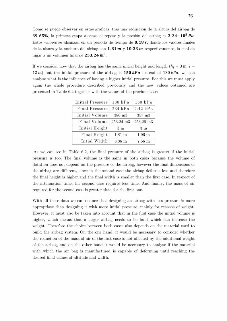
76
Como se puede observar en estas gráficas, tras una reducción de la altura del airbag de
𝟑𝟗. 𝟔𝟓%, la primera etapa alcanza el reposo y la presión del airbag es 𝟐. 𝟑𝟒 · 𝟏𝟎𝟓 𝑷𝒂.
Estos valores se alcanzan en un periodo de tiempo de 𝟎. 𝟏𝟖 𝒔, donde los valores finales
de la altura y la anchura del airbag son 𝟏. 𝟖𝟏 𝒎 y 𝟏𝟎. 𝟐𝟑 𝒎 respectivamente, lo cual da
lugar a un volumen final de 𝟐𝟓𝟑. 𝟐𝟒 𝒎𝟑.
If we consider now that the airbag has the same initial height and length (ℎ𝑖 = 3 𝑚 , 𝑙 =
12 𝑚) but the initial pressure of the airbag is 𝟏𝟓𝟎 𝒌𝑷𝒂 instead of 130 𝑘𝑃𝑎, we can
analyse what is the influence of having a higher initial pressure. For this we must apply
again the whole procedure described previously and the new values obtained are
presented in Table 6.2 together with the values of the previous case:
Initial Pressure 130 kPa 150 kPa
Final Pressure 234 kPa 2.42 kPa
Initial Volume 386 m3 357 m3
Final Volume 253.24 m3 253.26 m3
Initial H eight 3 m 3 m
Final H eight 1.81 m 1.96 m
Intial W idth 8.36 m 7.56 m
As we can see in Table 6.2, the final pressure of the airbag is greater if the initial
pressure is too. The final volume is the same in both cases because the volume of
flotation does not depend on the pressure of the airbag, however the final dimensions of
the airbag are different, since in the second case the airbag deforms less and therefore
the final height is higher and the final width is smaller than the first case. In respect of
the attenuation time, the second case requires less time. And finally, the mass of air
required for the second case is greater than for the first one.
With all these data we can deduce that designing an airbag with less pressure is more
appropriate than designing it with more initial pressure, mainly for reasons of weight.
However, it must also be taken into account that in the first case the initial volume is
higher, which means that a larger airbag needs to be built which can increase the
weight. Therefore the choice between both cases also depends on the material used to
build the airbag system. On the one hand, it would be necessary to consider whether
the reduction of the mass of air of the first case is not affected by the additional weight
of the airbag, and on the other hand it would be necessary to analyse if the material
with which the air bag is manufactured is capable of deforming until reaching the
desired final values of altitude and width.

77
CHAPTER 7. Conclusions
The main objective of this project was to carry out the preliminary design of the
recovery system of the first stage of a rocket. This recovery system was based on the
design of two main subsystems: the Parachute System and the Airbag System.
The design of the parachute system was based on a real parachute system used to
decelerate the first stage of the Ares X-I rocket. According to the data collected from
this application, we can conclude that the procedure used to calculate the required
parachute dimensions is adequate, since it is very close to the real case.
On the other hand, both the filling time and the estimated opening forces could not be
compared with the real values due to lack of information, but the experience with other
similar parachutes allows us to deduce that the estimated values are reasonable and
sufficient for the preliminary design, since they allow us to choose the material or
materials to manufacture the parachute system. However the time of inflation and the
opening forces are critical parameters that determine the success or failure of the
parachute performance, and therefore in a later refinement of the design would be
necessary to perform tests to ensure reliability.
Similarly, the parachute mass estimation was based on the correlation of mass values of
other parachutes. This method allows us to obtain the weight of the canopy in a fast
and effective way in preliminary design tasks. But the result of the weight estimation
obtained in this preliminary design phase is a very approximate value of the real one,
whose uncertainty depends fundamentally on the choice of materials of all the
components of the parachute. Therefore only from the last stages of design it can be
possible to obtain a more accurate estimate of this parameter, since a list of all the
components of the parachute with their dimensions and materials would require.
The design of the impact attenuation system is not included in the Ares I-X rocket
recovery system, but taking advantage of this example, it was proposed a possible
airbag system design that could be installed in the first stage of the rocket. The
purpose of this preliminary design was to check numerically the airbag behaviour
described in the theory and with this to validate the assumptions made. It was
necessary to modify the final phase of descent to be able to integrate a feasible airbag
system. For this purpose, a mechanism was included which consisted of an additional
parachute system to rotate the first stage from a vertical position to a horizontal
position. Despite the difficulty of modelling the airbag performance, it was possible to
obtain a sufficiently consistent impact attenuation system as a preliminary design. To
do the design of the airbag we didn’t consider the venting mechanism, but in a later
refinement of the design it would be necessary to study in detail the process of
attenuation, because the airbag really has a spring effect that makes the body oscillate,
and the system of relief valves is precisely the responsible for dampening this
movement.

78
Appendix A
A.1. H igh-Performance Parachute Types
Type
Constructed
shape
Inflated
Shape
Drag
Coefficient
Average
Angle of
Oscillation
Opening
Load
Factor
General
Application
D c/ D 0 DP/ D 0 CD 0 (D 0) Degrees CX
Flat circular 1.00
0.67
to
0.70
0.75
to
0.80
±10 to ±40 ~1.8 Descent
Conical 0.93 to 0.95 0.70
0.75
to
0.90
±10 to ±30 ~1.8 Descent
Biconical 0.90 to 0.95 0.70
0.75
to
0.92
±10 to ±30 ~1.8 Descent
Estended Skirt
(10%) 0.86
0.66
to
0.70
0.78
to
0.87
±10 to ±15 ~1.4 Descent
Extended Skirt
(14.3%) 0.81
0.66
to
0.70
0.75
to
0.90
±10 to ±15 ~1.4 Descent
Hyperflo 0.71 0.66
0.62
to
0.77
±10 to ±15 ~1.6 Descent
Guide Surface
(R ibbed) 0.63 0.62
0.28
to
0.42
0 to ±2 ~1.1 Stabilization Drogue
Guide Surface
(R ibless) 0.66 0.63
0.30
to
0.34
0 to ±3 ~1.4 Pilot, Drogue
Cross 1.15 to 1.19
0.66
to
0.72
0.60
to
0.78
0 to ±3 ~1.2 Descent, Deceleration
Flat R ibbon 1.00 0.67
0.45
to
0.50
0 to ±3 ~1.05 Pilot, Drogue,
Deceleration, Descent
Conical R ibbon
0.95
to
0.97
0.70
0.50
to
0.55
0 to ±3 ~1.05 Pilot, Drogue,
Deceleration, Descent
Hemisflo R ibbon 0.62 0.62
0.30
to
0.46
±2
1.00
to
1.30
Supersonic drogue
R ingslot 1.00
0.67
to
0.70
0.56
to
0.65
0 to ±5 ~1.05 Extraction,
Deceleration, Descent
R ingsail 1.16 0,69
0.75
to
0.90
±5 to ±10 ~1.10 Decent
Disc-Gap-Band 0.73 0.65
0.52
to
0.58
±10 to ±15 ~1.30 Supersonic, Drogue,
Descent
Hyperflo 1.00 0.80
0.35
to
0.44
0 to ±3
1.20
to
1.50
Supersonic, Drogue.

79
Solid Cloth Parachtues
Fla
t C
ircula
r P
ara
chute
s
The canopy is a regular polygon of N
sides, constructed as a flat surface with
a central vent. Its design is the basis
for most circular parachutes, other
types being variations in gore pattern
and general geometry. Flat circular
parachutes are simple and economical
to construct, handle and inspect, and
are often used in clusters. They are in
wide use for personnel and airdrop
applications. This parachute is very
reliable.
Conic
al
Para
chute
s
The canopy is constructed as the
surface of a regular pyramid of N sides
and base angle 𝜇. Its design is a minor
variation of the flat circular canopy.
The conical parachute is as simple and
economical to construct, handle and
inspect as the flat circular and serve
similar applications. As a result of
drop tests with models conducted in
1949, conical parachutes with up to 30o
cone angles showed approximately 10%
higher drag than solid flat parachutes
of the same surface area.
A.2. Skechtes and Applications
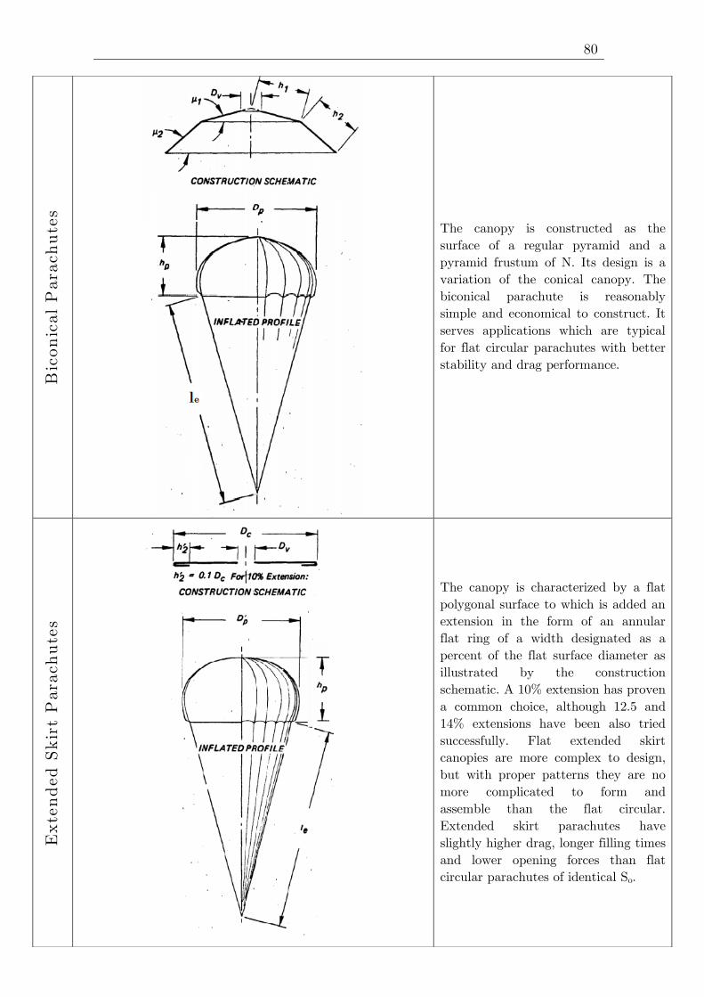
80
Bic
onic
al
Para
chute
s
The canopy is constructed as the
surface of a regular pyramid and a
pyramid frustum of N. Its design is a
variation of the conical canopy. The
biconical parachute is reasonably
simple and economical to construct. It
serves applications which are typical
for flat circular parachutes with better
stability and drag performance.
Exte
nded S
kir
t P
ara
chute
s
The canopy is characterized by a flat
polygonal surface to which is added an
extension in the form of an annular
flat ring of a width designated as a
percent of the flat surface diameter as
illustrated by the construction
schematic. A 10% extension has proven
a common choice, although 12.5 and
14% extensions have been also tried
successfully. Flat extended skirt
canopies are more complex to design,
but with proper patterns they are no
more complicated to form and
assemble than the flat circular.
Extended skirt parachutes have
slightly higher drag, longer filling times
and lower opening forces than flat
circular parachutes of identical So.

81
Hem
ispheri
cal
Para
chute
s
The constructed shape of this canopy
is a hemispherical surface. The gore is
designed so that the flat width
dimension is the horizontal arc
distance between radial seamlines. The
inflated shape approaches the
constructed profile under load. The
hemispherical parachute is more stable
than the flat circular type and is used
primarily for airdrop of supplies.
Rib
bed G
uid
e S
urf
ace P
ara
chute
s
The canopy is constructed with a
slightly rounded crown or roof, and an
inverted conical front or "guide
surface" extending from roof edge to
skirt hem. Ribs, placed between gores
in a plane with the suspension lines,
help to maintain the constructed
profile during operation. The guide
surface parachute was specifically
developed as a stabilization device for
bombs, mines, torpedoes and similar
bodies. Its good stability comes from
the abrupt flow separation edge of its
largest diameter and the guide surface
slope of the skirt. Low porosity cloth is
used in the roof and guide surfaces to
promote fast inflation and to help
maintain its characteristic shape. The
ribbed guide surface parachute is
reliable and very stable. However, it
has a low drag coefficient and is
difficult to manufacture.

82
Rib
less
Guid
e S
urf
ace P
ara
chute
s
In the ribless guide surface canopy, the
desired shape is obtained by modifying
the gore outline. The roof panel is
widened to extend around the edge of
the guide surface panel to the skirt
edge, eliminating the rib. The resulting
flow-separation edge is less abrupt,
accounting for a slightly higher
oscillation angle than the ribbed
version. A slit vent at the outer edge
of each guide surface panel also helps
to promote flow separation.
Construction is simplified by avoiding
the rib. Dimensions for roof and guide
surface panels depend upon diameter
and the number of gores in the canopy.
Cro
ss P
ara
chute
s
The cross parachute, a French
development, is finding increased use
for deceleration in applications that
require good stability and low cost.
The design is simple. The carnopy
consists of two identical cloth
rectangles, crossed and joined to each
other at the square intersection “t”
fcrm a flat surface having four equal
arms. Suspension lines are attached to
the outer edges of four arms. The
Cross parachute is similar in stability
performance and drag efficiency to the
ringslot parachute, but it has a
tendency to rotate. It is popular as a
deceleration perachute for ground
vehicles. Recent applications include
stabilization and deceleration of air
dropped n3val weapons and low rate of
descent, high altitude experiments.

83
Slotted Canopy Parachutes
Fla
t C
ircula
r R
ibbon P
ara
chute
s
The canopy is a flat circular design and
consists of concentric ribbons, usually 2
inches in width, supported by smaller
horizontally spaced tapes and radial
ribbons at gore edges. Ribbons and
tapes are accurately spaced to provide
the desired ratio of open space to solid
fabric over the entire canopy. Gores are
triangular and their dimensions are
determined in the same manner as for
the solid cloth flat circular parachute.
The flat circular ribbon parachute has a
lower drag efficiency than the solid
cloth parachutes. However, its stability
is excellent and the maximum opening
force is low in comparison. The canopy
is relatively slow in opening and its
performance reliability depends on
specific design parameters. Compared
to solid cloth parachute canopies, the
flat circular ribbon canopy is more
difficult to manufacture.
Conic
al
Rib
bon P
ara
chute
s
The constructed shape of this canopy is
obtained in the same manner as that
described for solid cloth conical
parachutes. Gores, like the flat circular
ribbon design, are composed of a grid of
horizontal ribbons spaced and retained
at close intervals by narrow vertical
tapes. Radial tapes which extend from
the vent to the skirt are sewn together
in the joining of adjacent gores.
The conical ribbon parachute shows
higher drag than the flat circular ribbon
just as the solid cloth conical parachute
does over the solid flat parachute of
equal area.

84
Hem
isflo R
ibbon P
ara
chute
s
The constructed shape of this canopy is
a spherical surface which continues 15
degrees past a hemisphere at the skirt
as shown. The canopy design retains
effective drag and stability performance
over the range from Mach 1.5 to 2.5,
although conical ribbon parachutes are
as good or better at speeds below Mach
1.5. Hemisflo parachute is used almost
exclusively for drogue applications
which require stabilization and
retardation at supersonic speeds.
Rin
gsl
ot
Para
chute
s
This parachute exists in flat and conical
designs. The canopy is constructed of
wide concentric cloth strips with
intervening slots in a manner similar to
the assembly of ribbon designs. Fewer
operations are required, simplifying
manufacture and reducing cost
compared with ribbon parachutes.
Performance characteristics are between
those of the ribbon and solid cloth
types. Ringslot parachutes are being
used for aircraft landing deceleration,
extraction of air drop equipment and
final recovery parachutes. Opening
reliability is comparable to ribbon
parachutes

85
Rin
gsa
il P
rachute
s
This parachute design is complex and
develops a unique shape from the
ccmbination of a curved basic profile
and fullness at the leading edge of
annular cloth rings. The constructed
profile is a circular arc, tangent to a 15o
cone at the apex and tangent to a 55o
cone at the skirt edge. The ringsail
canopy is constructed of wide
concentric cloth strips, spaced apart in
the upper crown with slots like the
ringslot, but adjacent over the
remainder of the canopy, obtaining
geometric porosity through crescent-
shaped slots resulting from the cloth
dimension between radials being longer
for the leading edge of each sail than
the trailing edge of the sail below it.
Dis
k-B
and-G
ap p
ara
chute
s
The disk-gap-band parachute was
developed to operate at very low
dynamic pressures at high altitudes and
supersonic speeds. This parachute is
designed to have better stability than a
solid flat canopy without loss of drag
efficiency. The right-angle change from
the band to the disk portion of the
canopy provides a discontinuity in the
surface shape and causes the interior
airflow to become separated around the
edge at all times. By adjusting the
width of the gap, the inside airflow of
the canopy can be controlled to
maximize the drag and maintain the
stability.

86
Hyperf
lo P
ara
chute
The Hyperflo type parachute is a
shaped parachute with a design
geometric shape like an inverted right
conical frustum. The decrease in drag
coefficient in the low supersonic speed
regime is somewhat compensated by an
increase in the projected canopy area in
this regime, giving the effect of
essentially constant drag area. This is
obviously a desirable characteristic and
an indication of satisfactory decelerator
performance at an operational
combination of low supersonic velocity
and dynamic pressures approaching 140
kPa.

87
Chara
cte
rist
icD
imensi
ons
Silk
Cott
on
Rayon
Nylo
nD
racon
Kevla
rG
lass
fib
er
Sta
ple
length
mm
400
- 140
0 m
120
- 6
30
Con
tinuou
sC
ontinuou
sC
ontinuou
sC
ontinuou
sC
ontinuou
s
Tensi
le s
trength
Kg/cm
2-
--
8300
840
026
000
24500
Tenacit
ygr/
den
ier
3,8
- 5
,22,
1 -
6,3
1,5
- 5
,0
6 -
96
- 9
20 -
22
7,7
Specific
weig
ht
gr/
cm3
1,3
41,5
21,5
1,1
41,3
81,4
42,
54
Ult
imate
elo
ngati
on
%13 -
31
3 -
715 -
25
25 -
40
12
- 20
3 -
53
Melt
ing p
oin
t0 C
150
230
170
- 2
30
248
252
454
730
Filam
ent
dia
mete
rm
m0,
0005
< 0
,001
0,00
050,
001
0,00
10,
0005
0,00
05
Wet
stre
ngth
%75
- 9
5110
- 130
45 -
55
85 -
90
95100
95 -
100
Resi
stance t
o:
--
--
--
-
Ult
ravio
let
rays
PG
PP
GD
E
Sto
rage, agin
gG
GG
EE
GE
Fungus,
bacte
ria
PP
PG
GG
E
Fla
me
PB
urn
sB
urn
sG
GG
E
P=
poo
r
G=
goo
d
E=
exce
llen
t
Appendix B

88
References
[1] National Oceanic and Atmospheric Administration, NASA, U.S. Air Force: “U.S.
Standard Atmosphere”. Documents Stock No. 003-017-00323-0, Washington, D.C.
20402, 1976.
[2] Theo W. Knacke: “Parachute Recovery Systems Design Manual”. Naval Weapons
Center, China Lake, California NWC TP 6575, 1992.
[3] D. J. Cockrell: “The Aerodynamics of Parachutes”. AGARDograph No.295,
Universty of Leicester, United Kingdom, July 1987.
[4] E. G. Ewing, H. W. Bixby, and T. W. Knacke, “Recovery Systems Design Guide”.
USAF AFFDL-TR-78-151, December 1978.
[5] R.C. Maydew and C. W. Peterson: “Design and Testing of High-Performance
Parachutes”. AGARDograph No. 319, Sandia National Laboratories, Albuquerque, New
Mexico 87185, U.S. November 1991.
[6] W. L. Garrard, M. L. Konicke, K. S. Wu, and K. K. Muramoto: “Measured and
Calculated Stress in a Ribbon Parachute Canopy”. AIAA Journal of Aircraft, Vol. 24,
No. 2, pp. 65 to 72, February 1987.
[7] W.D. Sundberg: “A New Solution Method for Steady-State Canopy Structural
Loads”. AIAA Paper. (AIAA 86-2489 CP).
[8] K. E. French: “A New Correlation of Parachute Weight Data”. AIAA Journal of
Spacecraft and Rockets, Vol. 8, No. 1, pp. 71-72, January 1971.
[9] W. Mueller: “Parachutes for Aircraft”. National Advisory Committee for
Aeronautics, NACA TM-450, October 1927.
[10] F. N. Scheubel: “Notes on the Opening Shock of a Parachute”. Progress Report
IRE-65, Foreign Exploitation Section, Intelligence (T-2), April 1946.
[11] K. E. French and Lockheed Aircraft Corp. Proceedings of the 1968 Aerodynamic
Deceleration Systems Conference: “The Initial Phase of Parachute Inflation”. U.S. Air
Force, El Centro, Calif. , USAF Report FTC-69-11, September 1968.
[12] D. L. Schilling and Lockheed Aircraft Corp: “A Method for Determining Parachute
Opening Shock Forces”. LAC Report 12543, August 1957.
[13] H. F. Freeman and I. Rosenberg: “High Altitude and High Airspeed Tests of
Standard Parachute Canopies”. U.S. Air Force, USAF Report AFFTC-TR-58-32,
October 1958.
[14] W.B. Pepper and J.F. Reed: “Parachute Study of Pressure Distribution in Wind
Tunnel Testing”. Journal of Aircraft, Vol. 10, No. 11, pp. 895-900, November 1976.
89
[15] Arnold AFB: “Aerodynamic Characteristics of Disk-Gap-Band Parachutes in the
Wake of Viking Entry Forebodies at Mach Numbers from 0.2 to 2.6”, AEDC-TR-72-78,
Tennessee, 1972.
[16] R. Brendt: “Supersonic Parachute Research”. U.S. Air Force, USAF Report ASD-
TR-66-236, July 1966.
[17] Barnhardt, Drayna, Nompelis, Candler, and Garrard: “Detached Eddy Simulations
of the MSL Parachute at Supersonic Conditions”, Proceedings of the 19th AIAA
Aerodynamic Decelerator Systems Technology Conference, Williamsburg, Virginia, May
2007.
[18] Paul V. Tartabini and Brett R. Starr: “Ares I-X Separation and Reentry
Trajectrory Analyses”. NASA Langley Research Center, Hampton, VA 23681, 2011.
[19] NASA’s Constellation Programm: “Ares I-X”. Press kit, October 2009.
[20] Edgar G. Ewing: “Ringsail Parachute Design”. Northrop Corporation Ventura
Division, Technical Report AFFDL-TR-72-3, pp. 57-58, January 1972.
[21] Daniel P. Raymer: “Aircraft Design: A Conceptual Approach”. Second Edition,
AIAA, Sylmar, California 1992.
[22] NASA flight test: “Ares I-X Launch Parachute Failure on Atlantic Ocean”.
Youtube https://www.youtube.com/watch?v=YSTuKzYuQ0Q, November 2009.
[23] Olivier L. de Weck, Sydney Do, Ricardo Robles, Joseph Pellicciotti, Tim Brady:
“An Airbag-Based Crew Impact Attenuation System for the Orion Crew Exploration
Vehicle”. AIAA 2009-6438, California, September 2009.
[24] Perry, J.A.: "Critical Flow Through Sharp-Edged Orifices" Transactions of the
American Society of Mechanical Engineers, pp. 757-764, October 1949.
[25] M. Cooper, R. Sinclair, J. Sanders: "Design and Testing of an Airbag Landing
Attenuator System for a Generic Crew Return Vehicle". AIAA 2005-1616, 18th
Aerodynamic Decelerator Systems Technology Conference and Seminar, 2005, Munich,
Germany.