
RBAFOI-171806 - housing component of CPI · Data frequency: I don ... I understand that HANA is...
98
1
Transcript of RBAFOI-171806 - housing component of CPI · Data frequency: I don ... I understand that HANA is...

1


1
From:Sent: Monday, 12 September 2016 8:39 AMTo:Cc:Subject: RE: Dun and Bradstreet company-level data [SEC=UNCLASSIFIED]
Hi
I think it’s going to be tricky to use company accounts data to construct estimates of property developer markups. There are a few issues to keep in mind…
Average versus marginal mark‐ups: I imagine the ABS wants to capture the mark‐up on new apartments.The company accounts (and ATO) data shown below capture average profits and hence average markups(i.e. across all built apartments and not just the newest ones). I guess you could make an assumption thatthe industry is perfectly competitive, in which case the average and the marginal mark‐up should be thesame. But I think the RIA intern note last year confirmed that the apartment building industry is highlyconcentrated.
Sampling bias: the company accounts data that we have are probably not designed for this exercise, as Isuspect the ABS will need data from some of the large apartment developers, like Meriton. The D&B dataonly include a small subset of residential construction firms and I think most of them are detached homebuilders. The D&B data are mainly focussed on firms that apply for debt and as I understand it the bigdevelopers like Meriton are largely equity financed and hence are not captured.
Data frequency: I don’t know of any mark‐up data that are quarterly. All the measures I know of are annual.
If the ABS wants to go down this path, then I think that ATO data on sales and profits would be the way to go. The ATO should be able to separately identify apartment builders (including the large developers) and the data should be quarterly. The publicly available ATO industry‐level data are here if you want to take a look at the types of data that are available: \\san1\er\Research\LaCavaG\Housing Supply\ATO Data.xlsx
Happy to meet this afternoon if you want to chat more.
Cheers,
| Economic Research Department RESERVE BANK OF AUSTRALIA | 65 Martin Place, Sydney NSW 2000
w: www.rba.gov.au
From: Sent: Friday, 9 September 2016 2:27 PM To: Cc: Subject: FW: Dun and Bradstreet company-level data [SEC=UNCLASSIFIED]
Hi ,
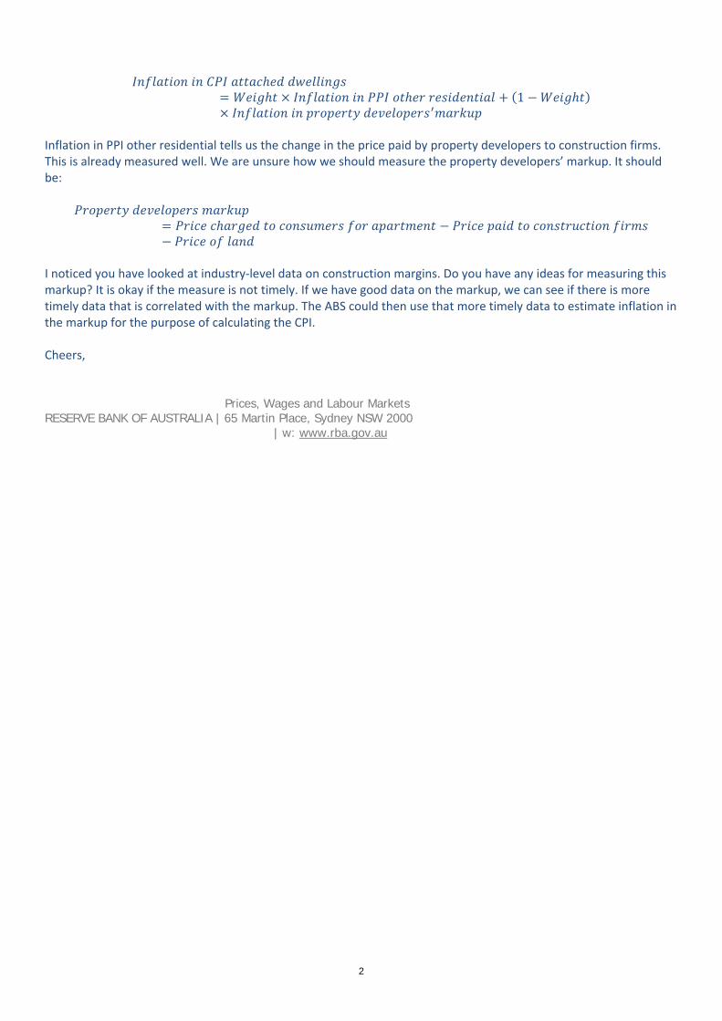
The ABS is currently doing work to incorporated attached dwellings into the CPI. Conceptually, we are trying to measure the price paid by the consumer to a property developer for an apartment, excluding land. The ABS is considering a ‘component cost’ approach, where it would calculate:
2
2
1
Inflation in PPI other residential tells us the change in the price paid by property developers to construction firms. This is already measured well. We are unsure how we should measure the property developers’ markup. It should be:
I noticed you have looked at industry‐level data on construction margins. Do you have any ideas for measuring this markup? It is okay if the measure is not timely. If we have good data on the markup, we can see if there is more timely data that is correlated with the markup. The ABS could then use that more timely data to estimate inflation in the markup for the purpose of calculating the CPI. Cheers,
Prices, Wages and Labour Markets RESERVE BANK OF AUSTRALIA | 65 Martin Place, Sydney NSW 2000
| w: www.rba.gov.au

1
From:Sent: Monday, 19 September 2016 11:58 AMTo:Subject: FW: Roadmap for CPI New dwelling purchase by owner-occupiers series
[SEC=UNCLASSIFIED]Attachments: Roadmap for CPI New dwelling purchase by owner-occupiers series.docx
Hi
The ABS’s work on measuring attached dwellings in the CPI has been progressing. Now that you are back from leave, I’d like to visit your desk to update you on what has happened so far. Please let me know a time that suits you.
Cheers,
From: Sent: Friday, 16 September 2016 9:56 AM To: Cc: @abs.gov.au'; @abs.gov.au;
Subject: FW: Roadmap for CPI New dwelling purchase by owner-occupiers series [SEC=UNCLASSIFIED]
Hi ,
I understand that HANA is interested in the ABS’s work on measuring attached dwellings in the CPI. I have attached the ABS’s draft paper. We have sent the ABS comments, which I will forward to you. and I also discussed the paper with the ABS on a call.
Our main point of contact at the ABS for this work is (CC’d). If you have questions, feel free to contact or myself.
Cheers,
Prices, Wages and Labour Markets RESERVE BANK OF AUSTRALIA | 65 Martin Place, Sydney NSW 2000
| w: www.rba.gov.au
From: @abs.gov.au] Sent: Thursday, 15 September 2016 3:55 PM To: Cc: Subject: Roadmap for CPI New dwelling purchase by owner-occupiers series
Hi ,
from our BACS area met with and from the Household/National Accounts group at the RBA. expressed interest in the work we are doing on measuring attached dwellings in the CPI.
Could you please send them the roadmap paper and pass on my contact details to Penny and Andrew.
Thanks
3

2
(See attached file: Roadmap for CPI New dwelling purchase by owner-occupiers series.docx)
Australian Bureau of Statistics
@abs.gov.au (W) www.abs.gov.au

ROADMAP FOR CPI NEW DWELLING PURCHASE BY OWNER-OCCUPIERS SERIES Prices branch August 2016
4

ROADMAP FOR CPI NEW DWELLING PURCHASE BY OWNER-OCCUPIERS SERIES Prices branch August 2016
Page 2 of 12
Purpose
The purpose of this paper is to outline the plan for the future measurement of the CPI series New dwelling purchase by owner-occupiers.
Known facts
• The Australian CPI is based on the acquisitions approach. For the purchase of dwellings this requires the measurement of price change for the net additions of dwellings (excluding land) by owner occupiers.
• The CPI series New dwelling purchase by owner-occupiers directly measures the price change for project homes. This is used as a proxy to capture the price change for attached dwellings where it is assumed they face similar supply and demand side influences.
• Pricing to constant quality is particularly problematic for measuring the price change in attached dwellings. • The residential building construction boom over the past couple of years has predominantly been driven by
an increase in construction activity of attached dwellings (see figures 1 and 2).
Recommendations
1. Implement the 'component cost' approach in the CPI in the December quarter 2016. 2. Further investigate the use of hedonic modelling for both attached dwellings and houses, with the view to
implement in the December quarter 2017 as part of the CPI 17th series review.
1. Concept and measurement
1.1 The CPI international manual states: "the treatment of owner-occupied housing is arguably the most difficult issue faced by CPI compilers. Ideally, the approach chosen should align with the conceptual basis that best satisfies the principal purpose of the CPI" (para. 10.4). The Australian CPI has adopted the acquisitions approach to align to the principle purpose of the CPI being a general measure of household inflation.
1.2 For owner-occupied housing this means the CPI measures the cost of net additions of dwellings to the household sector, which includes new homes (excluding land) and major improvements. Sales of houses that take place between households (generally established dwellings) are excluded so that the weights relate only to net additions to the housing stock.
1.3 The Australian CPI uses a matched model method for houses where project home builders are approached to obtain prices for a few specific models of project homes each quarter. The types of project homes selected are those most commonly constructed in each capital city. This method ensures both the pricing to constant quality and the exclusion of land.
1.4 Various methods are used by other countries to measure new dwelling purchase in their CPIs. Those on an acquisitions basis use similar methods to Australia. Those countries that aren't on an acquisitions basis use methods such as measuring gross mortgage interest repayments or a rental equivalence approach. The former method is similar to that used by the ABS in the Selected Living Cost Indexes series.

ROADMAP FOR CPI NEW DWELLING PURCHASE BY OWNER-OCCUPIERS SERIES Prices branch August 2016
Page 3 of 12
2. Attached dwellings
2.1 The recent residential building construction boom has predominantly been driven by an increase in the construction activity of attached dwellings. A recent RBA Bulletin article noted: "apartments have become an increasingly important contributor to new dwelling construction over recent years". Figures 1 and 2 show that for most cities the proportion of attached dwelling construction activity relative to total dwelling construction activity has increased since the recovery following the GFC. For Australia as a whole, this has seen attached dwelling construction activity going from contributing less than 30% of total dwelling construction activity post GFC, to over 40% in more recent times.
Figures 1 and 2: Value of attached dwellings building work compared to total dwelling building work (4 quarter average)
Source: 8752.0 - Building Activity, Australia, tables 21-29.
2.2 In the past, the CPI assumed that although price change for attached dwellings was not measured directly, it would be similar to the price change for project homes. This seemed a reasonable assumption based on the fact that both attached dwellings and houses faced similar input costs, both in terms of materials and labour, and also similar demand side influences, such as interest rates and property price growth.
2.3 Figure 3 compares the PPI's 3019 Other residential building construction series and the CPI's Project homes series. This comparison indicates the aforementioned assumption held up until the GFC. However, post GFC the series' started to diverge with the PPI series remaining lower than the CPI series. Following the GFC investment in large attached dwelling projects fell relative to new houses, as indicated by the proportions in figures 1 and 2. Figure 4 shows the recent boom in construction activity of attached dwellings has seen the series continue to diverge.

ROADMAP FOR CPI NEW DWELLING PURCHASE BY OWNER-OCCUPIERS SERIES Prices branch August 2016
Page 4 of 12
Figures 3 and 4: Indexes for PPI and CPI dwelling series'
3. Methods for measuring attached dwellings
3.1 The ABS is investigating two methods for the measurement of purchase of attached dwelling by owner-occupiers
Component cost
3.2 The component cost method is based on the principle that the price change for a product is based on the price change of the components (or inputs) that are used in the production of the product. This principle is adopted in the PPI series 3019 Other residential building construction. The Australian System of National Accounts (ASNA) also adopt this principle when measuring the output of non-market goods or services, such as those produced by the Health and Education industries. The ASNA states that: "when no prices for similar products exist, it may be necessary to value goods or services by the amount that it costs to produce them. This is the case for most non-market goods and services produced by general government units and non-profit institutions serving households" (para 3.43).
3.3 The PPI international manual describes the component cost method in detail and sites the ABS as an example (see appendix 1). For the CPI, the component cost method is discussed in the international manual in the context of quality adjustments and refers to it as the 'production cost approach'. The manual states: "a natural approach to quality adjustment is to adjust the price of an old item by an amount equal to the resource costs of the additional features of the new item" (para. 7.81). The manual goes onto say: "one distinction, then, between the use of producer cost estimates in the CPI and PPI is that only the former programme will add retail markups and indirect taxes" (para. 7.82).
3.4 The PPI series 3019 Other residential building construction aligns to the concept of measuring the purchase of attached dwellings in the CPI in that: it is measuring new dwellings only; pricing is to constant quality; and only the dwelling component is measured (i.e. land is excluded). What is missing from a CPI perspective are the impacts faced by the final consumer mentioned in paragraph 3.3.
3.5 Therefore, in adopting the component cost method in the CPI it is important to also capture the final retail margin and indirect taxes. The ABS is investigating combining the PPI series with a demand side indicator to capture

ROADMAP FOR CPI NEW DWELLING PURCHASE BY OWNER-OCCUPIERS SERIES Prices branch August 2016
Page 5 of 12
these impacts faced by the consumer. One option for this is the Residential Property Price Index's (RPPI) Attached dwellings series. The advantages of using this series is that it measures price change in attached dwellings only and reflects the demand for attached dwellings. Some disadvantages are it includes the value of land/location in the sale price, and captures established as well as new dwellings.
3.6 Figure 5 provides an example of what a CPI series for purchase of attached dwellings might look like compared to other relevant series. The series CPI attached* has a weight of 0.8 of the PPI series and 0.2 of the RPPI series. For the weighted 8 capital cities the CPI attached* series is lower than the CPI project homes series. Appendix 2 contains results for each of the capital cities. Further work (see below) is still required to investigate the suitability of this method.
Figure 5: Preliminary CPI series for purchase of attached dwellings.
3.7 This method has been replicated for houses using the PPI series Input to the house construction industry and the RPPI series Established house price index. Appendix 3 shows that this method is a reliable predictor of price change when compared to the CPI's Project homes series.
3.8 Following further investigation, it is proposed to implement this, or a similar method into the CPI for the December quarter 2016.
Hedonic model
3.9 The CPI international manual discusses the use of hedonic modelling in the context of quality adjustments. The manual states: "the (hedonic model) method should be applied where there are high ratios of non-comparable replacements and where the differences between the old and new items can be well defined by a large number of characteristics" (para. 7.120).
3.10 This description seems highly applicable to the case of attached dwellings where it is very unlikely for the same (in terms of quality) newly built attached dwelling to be purchased from one quarter to the next. In addition to this, attached dwellings also have a number of distinctive price determining characteristics such as geographic location and the number of bedrooms.

ROADMAP FOR CPI NEW DWELLING PURCHASE BY OWNER-OCCUPIERS SERIES Prices branch August 2016
Page 6 of 12
3.11 The ABS is investigating the use of a 'direct time dummy price index' as discussed in de Haan (2003). The ABS has received a test file from RP CoreLogic, which is the same data source used in the production of the RPPI. Using these data, variables that could be included in the hedonic model include location (e.g. suburb), number of bedrooms, bathrooms and car spaces, and floor space. As the test file includes dwelling type, an hedonic model could be used to measure price change for the purchase of both attached dwellings and houses in the CPI.
3.12 It is proposed that if testing indicates the use of an hedonic model is a suitable method for measuring price change for the purchase of attached dwellings and/or houses, then it will be implemented into the CPI as part of the 17th series review scheduled for the December quarter 2017.
4. Further work
• Determine the weight for attached dwellings as part of the CPI series New dwelling purchase by owner-occupiers.
• Consult with PPI and industry experts to understand the lower inflation experienced in attached dwellings compared to houses.
• Consult with industry to determine the most appropriate demand side indicator and the weight to apportion it.
• Continue to refine and test the hedonic model for both attached dwellings and houses.
References
Australian System of National Account: Concepts, Sources and Methods, (cat. no. 5216.0), 2015, ABS.
de Haan J ,2003 "Direct and Indirect Time Dummy Approaches to Hedonic Price Measurement", presented at the Ottawa Group, 2003
Consumer Price Index Manual: Theory and Practice, 2004, International Labour Organisation, paragraphs 7.81 - 7.124.
Producer Price Index Manual: Theory and Practice, 2004, International Labour Organisation, paragraphs 10.149 - 10.157.
Shoory, M. 2016, "The Growth of Apartment Construction in Australia, RBA Bulletin - June Quarter 2016

ROADMAP FOR CPI NEW DWELLING PURCHASE BY OWNER-OCCUPIERS SERIES Prices branch August 2016
Page 7 of 12
Appendix 1 Extract from PPI international manual
I.2 Residential building other than houses and non-residential building
10.149 The building output can be defined as a whole final structure or as a collection of particular elements that constitute the construction process. These elements should be narrowed down to include only those that would generally be covered in a standard construction contract between client and builder. Examples of excludable elements are any site works (such as demolition, land clearance, roads), external services (such as drainage, water and electricity connection), and design and other professional services.
10.150 Of the several compilation methods available, the ABS has chosen a method based on a breakdown of building construction into a set of common components. This so-called component cost method treats building output as a set of standardised homogeneous components representing subcontracted work-in-place. This and other methods for compiling building price indices are described in OECD and Eurostat (1997).
10.151 Typical projects were selected to represent construction activity in a range of functional categories, such as office buildings, shops, and factories. Each project was broken down into a set of standard well-defined components, each component consisting of a quantity, a unit rate, and a value (quantity multiplied by rate). The selection and analysis of projects was undertaken by a firm of quantity surveyors.
10.152 Projects are priced each period by updating the unit rate of each component while holding the quantity constant. The resultant component values are aggregated to produce a current-period project value. Project indices are weighted together to produce index numbers for strata, such as building function, region, and total industry.
10.153 Not all components need to be directly priced each period. First, pricing can focus on a subset of components that contribute to the bulk of the building cost. Second, it may be possible to use one item to represent several components that fall under the same building trade or that exhibit similar price behaviour. The unit rate (price) collected, for example, for one specification of the formwork to a suspended slab could represent several formwork components (say, formwork to slabs, columns, and beams). Finally, because the components are standardised, it will be possible for one specification to be applicable to several building types. Thus, instead of collecting a distinct set of prices for every component of each project, it may be possible to greatly reduce the number of prices collected by arriving at a group of representative items. For example, an office building, a shopping centre, a hospital, a hotel, and an apartment building will share a set of common components (the components will have different quantities and values for each project but share the same definition). For some of these common components, just one price may suffice for all of the projects. The items will need to be specified in considerable detail to enable consistent pricing from quarter to quarter. These element prices will then have to be aggregated to form the price of the building.
10.154 The ABS has contracted with a consultant to provide the unit rates for the building indices. The consultant, a large national quantity surveyor or cost consultant has access to up-to-date market prices for work-in-place and inputs. The consultant first builds up the unit rates from scratch, using prices and ratios for labour, materials, and plant. Profit margins and overheads are added. The rate is then modified according to up-to-date information on prices tendered for current projects. Every quarter the consultant provides 62 unit rates for each of nine geographic regions.
10.155 The ABS decided to obtain rates from a consultant, rather than collect rates through a survey of builders. This decision was based on economic considerations. The establishment of a collection for more than 550 items, with at least three different respondents per item, would have involved setting up more than 1,650 specifications, most of

ROADMAP FOR CPI NEW DWELLING PURCHASE BY OWNER-OCCUPIERS SERIES Prices branch August 2016
Page 8 of 12
which would have been complex models. This would have required significant time and resources. In addition, the maintenance of such a collection would be relatively complex and costly, ideally requiring the services of in-house building industry experts.
10.156 The advantages of the component cost method are (i) the index captures changes in productivity and subcontractor profit margins (unlike the simpler factor inputs method) by pricing work-in-place; (ii) it can be used for a range of structures, selected to best represent building activity; (iii) pricing is relatively simple and less resource intensive than the quoted price method (in which respondents provide prices for whole hypothetical structures), and consequently promises more plausible results; and (iv) it requires less information than hedonic methods.
10.157 The component cost method used by the ABS does not measure changes in the prime contractor’s profit margin - it is fixed at 5 percent. On the basis of information gained from interviews with contractors, the ABS determined 5 percent to be representative of a reasonable margin under normal conditions. This course of action was taken because the options for estimating the margin were judged to be highly subjective, or they involved the collection of very sensitive figures from respondents who are traditionally quite guarded about divulging such information. Work on developing a reliable measure for prime contractors’ margin is continuing, and if a reliable measure is developed it will be incorporated in the index.

ROADMAP FOR CPI NEW DWELLING PURCHASE BY OWNER-OCCUPIERS SERIES Prices branch August 2016
Page 9 of 12
Appendix 2 Component cost method preliminary results for each capital city

ROADMAP FOR CPI NEW DWELLING PURCHASE BY OWNER-OCCUPIERS SERIES Prices branch August 2016
Page 10 of 12

ROADMAP FOR CPI NEW DWELLING PURCHASE BY OWNER-OCCUPIERS SERIES Prices branch August 2016
Page 11 of 12
Appendix 3 Comparison of component cost method with the CPI's Project home series

ROADMAP FOR CPI NEW DWELLING PURCHASE BY OWNER-OCCUPIERS SERIES Prices branch August 2016
Page 12 of 12

1
From:Sent: Friday, 23 September 2016 4:59 PMTo:Cc:Subject: Draft email to on CPI attached dwellings. [SEC=UNCLASSIFIED]
Hi ,
This is the email I am planning to send to the ABS regarding CPI attached dwellings.
‐‐‐
Hi
My colleagues and I have given some thought to the measurement of attached dwellings in the CPI. I have written some fairly detailed comments below. Please let me know if you would like to discuss this in a call.
The ABS wants to measure the final price of an attached dwelling, excluding land. For a particular apartment, the price that should entire into the CPI calculation is:
My understanding is that high‐density property developers buy the land, pay a construction firm to build on the land, and then sell the attached dwelling to the consumer. We can write:
The first term is the property developer’s markup, and the second is PPI other residential. In the component cost approach, we calculate CPI attached as:
1
The outstanding question is how to measure inflation in the developer’s markup. Below I discuss three options for measuring this markup. The third option, of assuming the markup moves in line with PPI other residential, seems the most promising to us.
Option 1 – Using the residential property price index (RPPI) release
In the RPPI release contains an attached dwellings price index for each capital city. These indexes measure the price of the stock of dwellings, but they likely move similarly to the price of new dwellings. In our notation above, they
provide a reasonable measure of . However, it is less obvious that they provide a good measure of the markup
, which removes land prices and construction prices. Land prices tend to vary greatly over time, so there could be large divergences between the attached dwellings price index and the markup we are trying to estimate.
As far as I know, there are no housing price indexes that exclude land in Australia. In principle, such an index could be constructed, perhaps using data from each of the state valuers general. However, this seems like a challenging task. Perhaps this is why the RPPI release does not contain price indexes excluding land.
Option 2 – Estimating markups from profits
5

2
You could obtain data on the profits of property developers. Suppose, for argument’s sake, that the developer bought the land, paid the construction firm, and sold the dwelling all in the same quarter. Then the profit in that quarter would be:
Rearranging:
The right hand side is the markup. We can calculate it as long as we have data on profits and quantity of dwellings sold. The ATO publishes data on profits by industry (link). It might be possible to obtain more disaggregated data from the ATO, such as the profits of high‐density property developers. Another possibility is to use Dun & Bradstreet data, which we mentioned on the last call. However, having looked into this data further it seems to focus on detached home builders, not high density property developers. The big problem with estimating markups from profits is land prices. Property developers usually buy land a few years before they sell the dwelling. Consequently, their profit also reflects gains or losses on their portfolio of land, which could be substantial. Since changes in land prices would cause big movements in these estimates of the markup, it does not seem appropriate to use this method to measure CPI attached dwellings. If you can obtain data on the gains or losses that developers make on land, you could calculate better estimates of the markups. For publicly listed companies, you may be able to get this data from their financial statements. For other companies, you would have to compel them to give you this data. Option 3 – Impute markups from other components The ABS could assume that nsa inflation in the markup equals nsa inflation in PPI other residential. Under this assumption, CPI attached would equal PPI other residential. This assumption has a nice economic interpretation: it means developers’ markups are a constant fraction of CPI attached. This assumption seems roughly correct. It is true that the percentage markup may vary over time based on conditions on the housing market. However, in the absence of a good way to measure this markup, a constant percentage markup seems like the best option. Importantly, it ensures land prices do not affect CPI new dwellings, which we think is very important. This option would also be simple and transparent, and would not increase the amount of work needed to compile CPI. An alternative is to assume nsa inflation in the markup equals nsa inflation in CPI project homes. This is reasonable, but is a bit harder to explain, and does not have a nice interpretation as a constant percentage markup. Cheers,
| Prices, Wages and Labour Markets RESERVE BANK OF AUSTRALIA | 65 Martin Place, Sydney NSW 2000
| w: www.rba.gov.au

D17/317289 RESTRICTED 1
COST INFLATION FOR HIGH-RISE APARTMENT CONSTRUCTION
Inflation in the cost of constructing new apartments has been low in recent years, despite a large increase in activity. The containment of apartment construction costs can be partly explained by excess capacity in non-residential construction, particularly in the office sector. Industry contacts report that there is an overlap between the supply chains for apartment and office projects and that construction is typically undertaken by the same firms. Strong competition between these firms in recent years has limited tender price growth. Productivity improvements may have also helped to contain costs as high-rise construction activity has grown. In contrast to the containment of cost inflation in Sydney and Melbourne, costs have increased significantly in Brisbane alongside a sharper pick-up in activity.
The supply chain for detached house construction is quite different to that for high-rise apartment and commercial projects; the price of construction of detached houses has increased more notably in most markets in recent years despite only a modest increase in activity. Prices for newly constructed detached houses are included in the CPI but prices for apartments are not – as a result, the CPI has become less representative of dwelling purchase costs as apartments have accounted for an increasing share of new dwellings. A constructed measure of new dwelling costs that incorporates apartments suggests that the CPI measure of dwelling prices has probably overstated the true extent of housing inflation in recent years.
Introduction
Cost inflation for apartment construction has been low in recent years, both relative to history and to cost inflation for detached houses (Graph 1).1 Information from liaison suggests that the supply chain for apartment construction is relatively independent to that for detached homes and in fact overlaps with the supply chain for non-residential (particularly office) construction. Given this overlap, excess capacity among non-residential construction firms (which typically also undertake high-rise apartment construction) may have helped contain costs for apartment projects. Productivity improvements and strong competition among construction firms may have also contributed to the cost containment.
The distinction between cost pressures for detached houses and apartments is important – these costs flow on to prices and wages in the broader economy, and provide an indication of the capacity of different supply chains to deliver additional dwellings. There are also important implications for inflation measures. PPI output cost inflation for detached houses feeds in to the house purchase costs component of the CPI, whereas the purchase costs of new apartments and other dwellings are not currently reflected in the CPI despite the share of building approvals accounted for by these dwellings having increased notably (Graph 2). A constructed measure of new dwelling costs that incorporates apartments is lower than the CPI measure in recent years – see Box A.
Graph 1 Graph 2
1 The analysis in this note focuses on construction costs exclusively – the cost of the land or sites on which projects are constructed is not considered. In recent years, the cost of sites has reportedly increased sharply in the eastern capital cities, in contrast to the cost of constructed projects. As such, it can be implied that land costs have been the key driver of increases in final prices of new apartments (which is consistent with reports from liaison).
-10
-5
0
5
10
-10
-5
0
5
10
1998 2001 2004 2007 2010 2013 2016
PPI Output CostsYear-ended growth
Sources: ABS; RBA
Houses
Other residential% %
Non-residential
0
60
120
180
0
60
120
180
1995 1998 2001 2004 2007 2010 2013 2016
Residential Building Approvals* Annual
*Dots are for 2016 data to August, annualisedSources: ABS; RBA
'000 '000
Apartments
Detached houses
Total
Semi-detached
6

D17/317289 RESTRICTED 2
Recent trends and drivers of high-rise inflation
ABS measures of cost inflation indicate that growth in apartment construction prices has remained low in recent years. PPI output costs measure the cost of constructing an apartment project – this reflects the builders’ margin and input costs excluding land, but does not reflect the margin of the project developer. 2 PPI output cost inflation for ‘other residential’ construction (largely apartments, but also townhouses) has averaged only 1 per cent per year since 2011, well below the long-run average of 3 per cent (Graph 1). This is despite a large increase in apartment construction, with the annual number of building approvals doubling since 2011. By contrast, detached dwelling construction prices have increased notably in recent years despite only a modest increase in activity (see Shoory, 2015c and Shoory, 2016 for a detailed discussion of the drivers of new detached dwelling price inflation). Data on PPI output costs also indicates that cost inflation for ‘other residential’ and non-residential construction has been very similar over the past 20 years, and distinct from cost inflation for detached dwellings.3 Indeed, PPI output costs for detached houses have increased by almost three times as much those for ‘other residential’ dwellings and non-residential buildings since the beginning of the current interest rate easing cycle.
The containment of apartment costs can be partly explained by excess capacity in non-residential construction, particularly in the commercial sector where construction is typically undertaken by the same firms as those that build large or high-rise apartment projects. This is consistent with official data showing that both growth in costs and the level of costs are closely related for these two sectors (Graphs 1 & 8). Office buildings are more similar to apartment projects than other types of commercial projects (such as retail) and other non-residential developments (such as industrial), including in terms of scale, site location, site preparation and excavation. The scope for reallocation of activity (and labour) away from office construction to high rise apartments in recent years is apparent in the volume of office (and total commercial) construction approvals, which have been low relative to history and very low relative to high-rise apartment approvals (Graph 3). Contacts have reported that apartment projects have been a much more profitable use of land than office buildings in recent years, reflecting very strong demand for new apartments in inner-city areas.4, 5
2 The developer’s margin is reflected in the final price of apartments paid by buyers. In contrast to apartments, PPI output costs for detached house construction will typically closely resemble the final price because there is normally a builder only (and no developer).
3 Growth in implicit price deflators derived from building activity data also suggest a very close relationship between ‘other residential’ and non-residential construction costs from the early 2000s (see Graph B4 in Appendix B).
4 The return on investment for apartment projects is also generally much quicker than for office projects – the developer typically receives full payment immediately following settlement, while for offices and other forms of commercial construction the full payback is often not received until after at least a few years of tenancy.
5 According to RLB’s Crane Index for the June quarter 2016, 81 per cent of all cranes erected across the country were for residential projects, while only 7 were for commercial projects. The east coast accounted for 90 per cent of all cranes in Australia.
Graph 3
0.0
0.5
1.0
1.5
2.0
0.0
0.5
1.0
1.5
2.0
2000 2004 2008 2012 2016
Building Approvals - ValuePer cent of GDP, financial year
* Apartment buildings with 4 or more storeys** Component of commercialSources: ABS; RBA
Office buildings**
High-rise apartments*
% %
Total
Commercial

D17/317289 RESTRICTED 3
There are some similarities across the two sectors with finishing products and trades (such as those used for kitchens and bathrooms), though these represent a fairly small share of total costs.
Box A: Constructing a new measure for new dwelling cost inflation in the Consumer Price Index
The item ‘new dwelling purchases by owner-occupiers’ has an effective weight of 9 per cent in the Consumer Price Index (CPI), making it the largest single expenditure class in the basket. This component measures the cost of new detached dwellings only – specifically, the price of project homes purchased by owner-occupiers (excluding the cost of land). As the share of new dwellings accounted for by apartments has increased, this CPI series has become less representative of the new dwellings purchased and thus prices paid by home buyers. The ABS is working on incorporating apartments and other non-detached dwelling prices into the CPI, though the details for this new series and the timeline for its introduction are yet to be finalised.
I estimate a new dwelling costs series for the CPI that includes apartments and other non-detached dwellings (see Appendix A for a description of the methodology). This constructed measure, which incorporates PPI output costs for ‘other residential’ dwellings, suggests that the CPI measure of detached project homes has probably overstated the true extent of price pressures for buyers of new dwellings in recent years (Graph 4). The difference between the two series reflects the relative containment of ‘other residential’ construction costs, though the measures have converged in recent quarters as detached dwelling cost pressures have eased. The difference has been largest for Sydney, mostly due to the sharp increase in CPI new dwellings costs in 2013 and 2014 (Graph 5) (see Shoory, 2015 and Shoory, 2016). The constructed measure has been lower than CPI new dwelling costs in Melbourne but slightly higher in Brisbane in the past year, reflecting developments in ‘other residential’ PPI output costs in those cities (see Appendix A).
Graph 4 Graph 5
Differences by state
-2
0
2
4
6
-2
0
2
4
6
2002 2005 2008 2011 2014
Housing Cost InflationYear-ended
*Constructed using PPI output costs for 'other residential' construction and the CPI project home series,scaled by the value share of building approvals of different dwelling types Sources: ABS; RBA
CPI project homes (ABS series)
Dwelling costs (RBA constructed)*
% %
-2
0
2
4
6
8
-2
0
2
4
6
8
2002 2005 2008 2011 2014
Sydney Housing Cost InflationYear-ended
*Constructed using PPI output costs for 'other residential' construction and the CPI project home series, scaled by the value of building approvals by different dwelling typesSources: ABS; RBA
CPI project homes (ABS series)
Dwelling costs (RBA constructed)*
% %

D17/317289 RESTRICTED 4
Cost inflation for apartment construction has been contained in aggregate terms, though the scale of inflation has differed across the three eastern capital cities (PPI data are only available by state; these data are used as proxies for the capital cities, where almost all the high-rise construction activity takes place).
• Cost inflation has been lowest in Victoria, with costs having been flat or declining in recent years (Graph 7). This is consistent with liaison information – reports of productivity gains and strong competition in the tender market have been most commonly associated with Melbourne.
• Cost inflation in New South Wales has been moderate in recent years. However, industry contacts generally expect cost pressures to increase due to the strong pipeline of construction to be completed (including both residential and infrastructure projects).10 Indeed, some contacts believe the construction industry in Sydney is nearing capacity, and there have been reports that the commencement of some projects may be delayed because construction firms have a full workload.11,
Graph 6 Graph 7
In contrast to Sydney and Melbourne, apartment construction costs have grown significantly in Brisbane over the past few years as the industry has reportedly reached capacity. Among the three key eastern markets, Queensland is the only state where ‘other residential’ PPI output costs have grown by more than those for detached houses (see Appendix B). This is consistent with liaison messages – contacts have reported that the sharp increase in high-rise construction since mid 2013 has driven large cost increases, and that as a result several planned projects will not proceed to construction. The cost pressures in Brisbane have likely been exacerbated by the scale of the increase in activity compared to the size of the existing market. It is also possible that the construction cycle is young enough that productivity improvements have not yet been achieved (as in Melbourne). In addition, the pool of available resources is smaller than in Sydney and Melbourne. For instance, one contact reported that it was almost impossible to source a crane in south-east Queensland in late 2015, and some have suggested that the large pipeline of non-residential construction underway for the 2018 Commonwealth Games (in the Gold Coast) has stretched the availability of construction firms. Contacts have reported that suitable labour has been in short supply and rates for tradespeople have increased significantly, with the slowdown in the mining sector not appearing to have materially improved labour availability.12, Cost pressures are likely to remain elevated in Brisbane over the coming year as a large pipeline of work is completed. However, these pressures may ease somewhat in subsequent years following a weakening demand from apartment buyers and a slowdown in project announcements in the past year.
10 RLB forecasts construction costs in Sydney to grow by up to 5 per cent annually in 2016 and 2017 (Table B1 in Appendix B). 11 Consistent with these reports, ABS data show that the volume of ‘other residential’ work that is ‘approved but not yet commenced’ has
increased in New South Wales in the past year. 12 One contact commented that the slowdown in the mining sector released less labour into the Queensland construction industry than
expected, speculating that this was due to a large share of the workers being FIFOs from interstate (particularly Sydney) who had subsequently returned home rather than transitioning into construction in Queensland.
0.0
0.5
1.0
1.5
0.0
0.5
1.0
1.5
2000 2004 2008 2012 2016
High-rise Apartment Building Approvals - Value* Per cent of GSP, financial year
* Apartment buildings with 4 or more storeysSources: ABS; RBA
VIC
NSW
% %
QLD
-15
-10
-5
0
5
10
15
-15
-10
-5
0
5
10
15
2001 2004 2007 2010 2013 2016
PPI Output Costs - 'Other Residential' Year-ended growth
Sources: ABS; RBA
New South Wales
Victoria
% %
Queensland
Australia
Graph 8

D17/317289 RESTRICTED 5
In addition to differences in cost growth, the level of costs for constructing high-rise projects differs across markets. Data from quantity surveyor Rider Levett Bucknall (RLB) indicate that construction costs are typically higher in Sydney relative to Melbourne and Brisbane, which is consistent other reports from liaison (Graph 8). The higher costs in Sydney partly reflect site access costs and restrictions – contacts report that suitable sites for apartment projects are less readily available in Sydney, and those that are available are typically more difficult to build on and/or zoned for lower heights than would be possible in Melbourne or Brisbane. Notwithstanding the differences across markets, these levels data show the close relationship between apartment and office construction costs in several cities (both Australian and international), supporting the notion that excess capacity in office construction can facilitate cost containment for apartment projects.
Outlook Apartment construction costs in Sydney and Melbourne have been contained in recent years by a combination of excess capacity in office construction, competition between commercial construction firms and productivity improvements. Over the coming two years, cost pressures are likely to increase due to the large pipeline of construction to be completed, particularly in Sydney where some contacts have suggested the industry is close to reaching capacity. Cost pressures are likely to remain elevated in Brisbane over the coming year, though a weakening in demand and a slowdown in new project announcements may see these pressures ease once projects under construction have been completed. However, the impact of apartment construction cost increases on measures of headline inflation will ultimately depend on how and when the ABS includes these costs in the CPI.
/Regional and Industry Analysis/Economic Analysis/ 6 October 2016
13 See Shoory (2015a) and Shoory (2015b) for more details on site availability in Sydney.
0
1
2
3
0
1
2
3
High-rise Construction Costs* December quarter 2015, per square metre
$US '000
$US '000
* Converted to $US from local currencies using average market exchange rates over December quarter 2015 **Grade A officesSources: RLB; RBA
Apartments
Offices**

D17/317289 RESTRICTED 6
References Doyle & Langcake (2014), Labour and Materials Intensity of House and Apartment Construction Shoory (2016), ‘Box a: New Dwelling Costs and Prices’, Liaison on Current Conditions – July 2016 Shoory (2015a), The Apartment Approvals Process Shoory (2015b), Recent Developments in Apartment Markets Shoory (2015c), Recent Drivers of New Dwelling Price Inflation
Appendix A: Methodology of constructing residential cost inflation
CPI house purchase costs currently reflect detached dwellings only. We can estimate a CPI-style ‘dwelling purchase costs’ price index that includes both detached and high-density dwellings using information available in the PPI. This index is constructed by combining the PPI output cost series for ‘other residential’ dwellings and the existing CPI house purchase costs series for detached houses, weighting each by their share of building approvals.
• Approvals for semi-detached dwellings are combined with those for detached houses because the construction methods employed are more similar than those used for apartments and the CPI new dwelling series is likely more representative of costs for those dwellings. (Note: the PPI output series for ‘other residential’ dwellings includes semi-detached.)
• Approvals for high-rise and low-rise apartments are combined.
• The index is calculated using value of building approvals. Substituting this for the number of approvals instead only makes a slight difference.
• The data are quarterly and no lags are incorporated.
• For the state/city specific charts, the CPI data are for the capital cities (Sydney, Melbourne, Brisbane) but the PPI output series are only broken down by state.
• Because PPI output costs exclude the developer’s margin (which is reflected in the final price paid by buyers), this method assumes that these margins have remained constant over time.
• The ABS is considering two ways of incorporating non-detached dwellings into the CPI: an input approach (estimate prices using PPI measures of input costs and a measure of developers’ margins) possibly as early as the December quarter 2016 or a hedonic approach (using microdata purchased from RP Core Logic, the ABS would regress the price of a new dwelling on the dwelling’s characteristics and a time dummy – the timeframe for this approach is unclear).
Graph A1 Graph A2
-4
-2
0
2
4
6
8
-4
-2
0
2
4
6
8
2002 2005 2008 2011 2014
Melbourne Housing Cost InflationYear-ended
*Constructed using PPI output costs for 'other residential' construction and the CPI project home series, scaled by the value share of building approvals of different dwelling typesSources: ABS; RBA
CPI project homes (ABS series)
Dwelling costs(RBA constructed)*
% %
-5
0
5
10
-5
0
5
10
2002 2005 2008 2011 2014
Brisbane Housing Cost InflationYear-ended
CPI project homes (ABS series)
Dwelling Costs (RBA constructed)*
% %
*Constructed using PPI output costs for 'other residential' construction and the CPI project home series, scaled by the value share of building approvals of different dwelling typesSources: ABS; RBA

D17/317289 RESTRICTED 8
Graph B7 Graph B8
0
50
100
150
200
250
0
50
100
150
200
2502000-09 2010 onwards
High-rise Residential ConstructionNumber of completions; includes projects under construction
No. No.
* Buildings over 100 metresSources: The Skyscraper Center; RBA
20
30
40
50
20
30
40
50
2000-09 2010 onwards
High-rise Residential ConstructionAverage floors per project; includes projects under construction
Floors Floors
* Buildings over 100 metres; includes mixed-useSources: The Skyscraper Center; RBA

Price and Wage Developments | Statement on Monetary Policy – November 2016 | RBA
https://www.rba.gov.au/publications/smp/2016/nov/price-and-wage-developments.html[13/10/2017 2:17:39 PM]
About Us Monetary Policy Market Operations Financial Stability
Payments & Infrastructure Financial Services Banknotes
In PublicationsStatement on Monetary Policy – November 2016
5. Price and Wage Developments
InflationA number of factors have contributed to continued low inflation. Spare capacity inthe labour market is restraining wage growth. Heightened competition in anumber of product markets is also contributing to low inflation outcomes.Furthermore, measures of inflation expectations have declined over the past year,which may be influencing price and wage-setting behaviour. Lower inflationexpectations may, in part, reflect the effect of the large fall in oil prices andcommodity prices more generally, over recent years. The adjustment to thedecline in the terms of trade over recent years has also weighed on nominalgrowth – including via wages and margins – and the effect of the decline in theterms of trade is evident in the particularly low inflation outcomes in Perth. Thedepreciation of the exchange rate since 2013 has put upward pressure on tradableprices in recent years.
The September quarter inflation data were broadly in line with forecasts made atthe time of the August Statement. Headline consumer price inflation increased alittle in year-ended terms to 1.3 per cent (Graph 5.1; Table 5.1). Volatile itemsadded to headline inflation in the quarter; higher fruit and vegetable prices causedby supply disruptions more than offset a decline in fuel prices. In year-endedterms, measures of underlying inflation have been around 1½ per cent over thepast few quarters (Graph 5.2). Non-tradable inflation was little changed in theSeptember quarter (Graph 5.3). It continues to be weighed down by low pricegrowth of market services and rents.
Prices for tradable items (excluding volatile items and tobacco) declined a little inthe quarter and were unchanged over the year.
Low inflation has been broad based across the CPI components. Less than one-quarter of the components of the CPI basket have price growth above their long-run average (Graph 5.4). This includes tobacco, childcare and insurance. Tobacco
Home › Publications › Statement on Monetary Policy › 2016 › November › Price and Wage Developments
Careers Education Media Q&A Glossary Contacts
Media Releases Speeches Publications Statistics Chart Pack
Minutes
Statement on MonetaryPolicy
2017
2016
November
August
May
February
Boxes
2015
2014
2013
2012
2011
2001–2010
1997–2000
Financial Stability Review
Bulletin
Annual Reports
Corporate Plan
7

Price and Wage Developments | Statement on Monetary Policy – November 2016 | RBA
https://www.rba.gov.au/publications/smp/2016/nov/price-and-wage-developments.html[13/10/2017 2:17:39 PM]
has contributed around 1/3 percentage point to CPI inflation over the past year,largely due to increased excise taxes. Offsetting this, lower automotive fuel priceshave subtracted around 1/3 percentage point from CPI inflation over the year.More recently, fuel prices have increased as global oil prices have moved higher,which if sustained will add a little to headline inflation.
Labour costs are an important determinant of inflation and there has been broad-based weakness in measures of labour cost growth (see below). The implicationsfor inflation depend on how labour costs evolve relative to productivity. Unitlabour costs have now been little changed for around five years, as low wagegrowth has been offset by productivity gains (Graph 5.5). Labour costs accountfor around one-half of final prices for market services; consistent with this, marketservices inflation is around its lowest level over the inflation-targeting period. Inparticular, prices for telecommunication equipment & services have fallen sharplyover the past two years, reflecting increased competition and technologicalchange in the industry.
In the retail sector, heightened competition has largely offset the effect of thehigher cost of imported goods owing to the earlier depreciation of the exchangerate (Graph 5.6). These competitive pressures largely reflect the entry of overseasretailers. In response to competitive pressures, firms have made efforts toreduce cost pressures along the supply chain, which is reflected in a pick-up overrecent years in multifactor productivity growth in the wholesale and retail tradeindustries. Low wage growth has also contributed to low retail sector inflation. Theeffect of heightened competitive pressures on inflation is expected to wane overtime, although the point at which this occurs is uncertain.
Rent inflation is well below its inflation-targeting average (Graph 5.7). Rents havecontinued to fall in Perth, in line with weak economic activity and a markedslowdown in population growth. In other capital cities, an increase in the supply ofhousing, particularly apartments, has contributed to low rent inflation. Furtherincreases in housing supply over coming years is expected to result in a protractedperiod of low rent inflation.
New dwelling price inflation has declined in year-ended terms since mid 2015. Thisslowing has been fairly broad based across all cities, which appears somewhat atodds with the continued solid level of activity in detached housing construction inSydney and Melbourne. New dwelling costs are currently measured as the cost ofconstructing a new detached house and, as such, do not capture the cost ofbuilding an apartment where a lot of the activity has been concentrated. Materialand labour cost growth remains subdued, although liaison has suggested thatthere are some pockets of wage pressures, such as for bricklayers, in the easternstates. One potential explanation for subdued price pressures in thedetached housing market is that heightened competition has meant builders havebeen focusing on reducing costs.
Research DiscussionPapers
Conferences
Workshops
Submissions
Consultations
Order Form
[1]
[2]
rsdpdl
Sticky Note
Marked set by rsdpdl

Price and Wage Developments | Statement on Monetary Policy – November 2016 | RBA
https://www.rba.gov.au/publications/smp/2016/nov/price-and-wage-developments.html[13/10/2017 2:17:39 PM]
Utilities inflation is low relative to its inflation-targeting average. This largelyreflects regulatory decisions, which have approved much smaller price rises thanthose that were granted in the late 2000s. Gas and water & sewerage inflationover the year is low relative to the inflation targeting period, and there were largeprice falls in the September quarter for a number of cities. In contrast, there werelarge increases in electricity prices in Sydney and Adelaide in the Septemberquarter, driven in part by higher wholesale electricity costs; these wholesale costpressures are expected to flow through to Melbourne retail electricity prices in theMarch quarter. Excluding utilities, administered price inflation is only a little belowaverage levels.
Labour CostsWage growth appears to have stabilised, albeit at a low level (Graph 5.8). Growthin the private sector wage price index (WPI) has been stable for six quarters at anannualised pace of around 2 per cent. Year-ended growth in the public sector WPIalso appears to have stabilised around 2½ per cent since early 2015. Wagegrowth is lower than average across all industries and states and the dispersion inwage growth across industries is at its lowest level since the series began in thelate 1990s. Broader measures of labour costs also appear to have stabilised oreven picked up. Growth in average earnings per hour from the national accounts(AENA) – which also captures non-wage costs as well as the effect of promotionsand changes in the composition of employment – has picked up in recentquarters. There has been little change to unit labour costs over recent years asgrowth in labour costs have been matched by productivity gains.
The weakness in wage growth over recent years reflects a number of factors,some specific to Australia and others also evident in other countries. First, therehas been some spare capacity in the labour market putting downward pressure onwage growth. While it is difficult to be precise, it is estimated that the currentunemployment rate is a bit over ½ percentage point higher than full employment.Furthermore, as has been the case in other advanced economies in recent years,it appears that there has been some change in the historical relationship betweenwage growth and measures of spare capacity. There are a range of plausiblestructural and cyclical explanations for this: increased labour market flexibility mayhave provided firms with greater scope to adjust wages in response to changes innominal revenue growth; workers may be putting more emphasis on job securitythan higher wage claims as a result of the global financial crisis or structuralchange; and/ or reduced workers' pricing power as a result of increasedcompetitive pressure from globalisation and technology. The extent to whichthese factors persist will determine how quickly wage growth picks up as labourmarket conditions improve.
A second influence on wage setting has been low outcomes for headline inflationover the past couple of years and the associated decline in inflation expectations
[3]

Price and Wage Developments | Statement on Monetary Policy – November 2016 | RBA
https://www.rba.gov.au/publications/smp/2016/nov/price-and-wage-developments.html[13/10/2017 2:17:39 PM]
(at least over the short to medium term). Workers may have agreed to smallerwage increases given low actual and expected inflation.
A third factor weighing on wages growth has been increased efforts by firms tocontain growth in labour costs. Over recent years, the sharp fall in the terms oftrade, heightened competition (such as in the retail market) and spare productivecapacity in product markets has weighed on firms' output prices.
Low wage growth in recent years has helped the economy adjust to the lowerterms of trade. Combined with the depreciation of the nominal exchange ratesince 2013, low growth in labour costs has improved Australia's internationalcompetitiveness. This is in contrast to the earlier period of sharply risingcommodity prices and mining investment, during which Australia's unit labour costgrowth outpaced that in many comparable countries, contributing to a decline inAustralia's international competitiveness.
As the economy continues the transition away from mining-led activity, there arelikely to be further adjustments to relative wages. Following a period of beingabove average, wage growth is currently lowest in industries and states that aremore exposed to the end of the terms of trade and mining investment boom, andrelative wages in these industries and states have started to turn lower (Graph5.9). Liaison suggests that the movement of workers from higher-paying mining-related jobs to lower-paying jobs elsewhere in the economy is well advanced.
Analysis of micro-level WPI data from the Australian Bureau of Statistics indicatesthere has been both a decline in the frequency of wage increases and in theaverage size of the increases in recent years. In particular, the share of jobsthat experienced wage growth in excess of 4 per cent has fallen sharply, largelyreflecting a decline in large wage rises in mining-related jobs (Graph 5.10).Workers in around half of all jobs have received a wage increase of between 2–3 per cent. Only a small share of jobs has experienced a decline in wages,indicating downward nominal wage rigidity.
Inflation ExpectationsMeasures of inflation expectations have declined over the past year, consistentwith low outcomes for CPI inflation, although consumers' short-term inflationexpectations have been little changed over the past year. More recently, one- yearahead inflation swaps have increased a little (Graph 5.11).
Survey-based measures of long-term inflation expectations remain around themid-point of the inflation target (Graph 5.12). After falling sharply earlier in theyear, financial market measures of inflation expectations have been more stable oflate. Five-to-ten year inflation swaps, which capture expected average inflationover the period five-to-ten years ahead, have picked up modestly over the pastfew months, while inflation expectations based on 10-year bonds have been little
[4]
Price and Wage Developments | Statement on Monetary Policy – November 2016 | RBA
https://www.rba.gov.au/publications/smp/2016/nov/price-and-wage-developments.html[13/10/2017 2:17:39 PM]
Copyright Disclaimer Judicial Notice Privacy Accessibility Scams
Share
changed since June at low levels. The 10-year indexed bond measure has declinedover the past year by more than the five-to-ten year inflation swap measure. Thisis in part because it is an expected average inflation rate over the next 10 yearsand so is affected by expected low inflation in the near term.
The financial market measures of inflation expectations can be affected by factorsother than changes in investors' perceptions of expected future inflation, such aschanges in the premium that investors' demand to bear inflation risk. Changes inthis premium affect both the inflation swaps and bond-based measure of inflationexpectations. The bond-based measure is also affected by changes in the liquidityof inflation-indexed bonds relative to nominal bonds. Regulatory changes since2008 may have led to a relative deterioration in liquidity of inflation-indexedbonds; this would tend to raise the yield on indexed bonds and depress theimplied inflation rate. Bank estimates suggest that much of the decline in thebond-based measure over the past 12 months is due to changes in the liquidityand inflation risk premia rather than long-term expectations of inflation, whichhave been relatively little changed.
Footnotes
Continue to ‘Economic Outlook’ →
For a more detailed discussion, see Ballantyne A and S Langcake (2016), ‘Why HasRetail Inflation Been So Low?’, RBA Bulletin, June, pp 9–17.
[1]
The wage price index (WPI) shows low wage inflation for the construction industry,however this measure also includes wages for workers in non-residential andengineering construction where activity has been weaker. The WPI also does notmeasure income growth for subcontractors, who make up a high share of workers inthe detached housing industry. There is some tentative evidence that the incomegrowth of these subcontractors has picked up.
[2]
See Lowe, P (2016), ‘Inflation and Monetary Policy’, Address to Citi's 8th AnnualAustralian & New Zealand Investment Conference, Sydney, 18 October.
[3]
Further analysis of these data will be available in the September quarter 2016 WagePrice Index release (released 16 November 2016).
[4]

1
From:Sent: Monday, 31 October 2016 2:34 PMTo:Cc:Subject: FW: Construction skirmish notes [SEC=UNCLASSIFIED]Attachments: Construction skirmish_Final.docx
Hi ,
The ABS sent us a summary of its interviews with house and apartment builders. Hope you find the results interesting. Please let us know if you have any thoughts.
Cheers,
Prices, Wages and Labour Markets RESERVE BANK OF AUSTRALIA | 65 Martin Place, Sydney NSW 2000
| w: www.rba.gov.au
From: @abs.gov.au] Sent: Monday, 31 October 2016 11:57 AM To: Cc: Subject: Construction skirmish notes
Hi all
It was good to meet with you all again today for the Prices briefing.
As promised, attached below is the note that we have put together on the Construction skirmish.
Feel free to pass this note onto anyone else within the RBA that might be interested, and of course if you have any questions, please let me know.
Cheers
Producer Price Indexes | Macroeconomic Statistics Division | Australian Bureau of Statistics
@abs.gov.au (W) www.abs.gov.au
(See attached file: Construction skirmish_Final.docx)
8

Construction skirmish - September quarter 2016
Context
There has been considerable interest in the Construction industry recently following the downturn in the mining boom, concerns about rising property prices, and risks of oversupply in the attached dwellings market.
Each quarter, after the release of the Consumer Price Index and the Producer Price Indexes the Reserve Bank of Australia (RBA) meets with staff from the Prices Branch for a Price’s debrief of the quarter. During the June quarter 2016 debrief the Prices Branch agreed to undertake a skirmish of the construction industry in order to gain a better understanding of current conditions as well as understanding the pricing mechanism within the industry.
Details of the skirmish
Over the past few months, the ABS Prices branch met with a sample of key players in the industry across both the east coast and west coast including:
- 10 Project Home Builders - 1 Property Developer - 1 Quantity surveyor
The discussions centred around the following 5 main themes:
1. Current state of the housing market and outlook2. How are Construction prices set, including the determination of margins3. The pass through of input costs to the final price4. Developments in the Labour market5. Innovation and Productivity Improvements in the Industry
Findings
Overall, the discussions were useful and provided information is generally not available through the ABS regular data collection. Most of this was anecdotal in nature however there were certainly a number of common themes which resonated throughout the discussions. These are summarised below:
Current State of the market:
• New South Wales builders generally noted that the market was relatively steady at the moment.However some also mentioned that sales had slowed recently.
• The housing market in Victoria was considered by builders to be moderate to steady. Somebuilders noted that the market was slowing and competition amongst builders was high.
• The market in WA is in decline following the downturn in mining which has impacted on demand.Volume of sales has dropped off considerably from previous years. Builders did not expect marketconditions to improve in the near future.
• Across the board it did not appear that project home builders had seen or were aware of anyimpacts of the boom in apartment sales on sales of detached houses. Some noted that that theyare competing in different markets. For example, Project home builders tend to be competing inthe market for second and third home buyers. Moreover, apartments are also mostly concentratedin the CBD while detached houses are generally located in the outer suburbs and so are not indirect competition.
9

How are Construction prices set, including the determination of margins
• When setting final prices, builders are able to anticipate future increases in costs of labour and materials by factoring them into current prices. Cost of materials are generally reviewed with suppliers once a year and changes in labour costs as a result of EBA’s and subcontractor rates also come through once a year and can be factored into the current prices. Depending on the builder, sophisticated forecast models may be used, whereas, others use informed judgement or experience to estimate future increases.
• Builders noted that the biggest unknown variable in setting prices is the Construction time. Delays in construction process as a result of planning/approvals process, and weather were difficult to anticipate and impacted on margins and profitability.
• In setting margins, most builders indicated they targeted a gross margin as opposed to a net margin. That is, they target a margin on each build which will allow them to cover other expenses such as office administration costs, display home cost, marketing etc…
• Depending on how competitive the market in the region is, builders will target price points, which will determine their margin. Builders in competitive markets will either target lower price points to achieve greater profit through volume of sales
• Once a margin has been determined, they are generally inflexible. Project home builders noted that they rarely cut their gross margins. Even during periods where activity is subdued. Builders also noted that they rarely ever dropped advertised prices. Instead they looked at cutting other costs within the business such as reducing the number of staff in the office, number of display homes
• Competition for sales is generally carried out in the form of bonus offers, upgrades or inclusions. Higher margins are made on homes with upgrades or inclusions.
• On the attached dwellings side, final prices are determined based on what the developer believes the market can handle in terms of a final price. This takes into account a number of different factors including the cost of the build, land availability, financing costs. One further consideration for the developer is both the ‘hurdle rate’ as well as the ‘hurdle number’ the minimum number of off the plan sales required to proceed with the project.
• A key difference on the attached dwellings is that both prices and margins tend to be more flexible. It was noted here that developers will adapt to the current market. For example, developers can reconfigure floor plans and inclusions in order to reflect demand, even while the apartment is being constructed.
• There are significant differences in materials and labour used compared to Project homes. Attached dwellings have significant costs on things like cranes, scaffolding, engineering services and other skilled labour. In addition, the planning and approvals process is significantly longer and more complex.
Pass through of costs
• Project Home builders noted that pass through of material costs and labour tended to take place gradually over time. Builders tend to have long term agreements with suppliers (up-to 12 months), which are known and would have already been factored into the cost of construction earlier. As competition amongst builders is very high and consumers are generally price sensitive, builders have been reluctant to pass on cost increases quickly. Changes in exchange rates generally don’t have much of an effect in the short term on prices as long term contracts or hedging strategies are in place

• Labour costs have been relatively subdued, with builders noting that there has been a good supply of tradesman available and very little pressure on wage rates. For some Trades (particularly bricklayers), rates have increased dramatically over the recent period.
• Overall, material costs increases have been relatively small in recent periods, and some builders even noted that they have been able to negotiate price falls for certain materials. On the attached dwellings side, developers noted that pass through of costs tend to be smaller in comparison to the project homes side. This is due to a number of factors including:
- The ability of the developers to enter into longer term contract which hedge against price increases.
- Some of the bigger builders tend to have a lot of stock on hand which insulates them from any short term price increases.
- Developers are often able to negotiate significant discounts with their suppliers when ordering bulk especially when they have a number of projects operating at the one time.
Developments in the labour market
• Builders noted that the supply of labour is quite good at the moment which is keeping wages and contractor rates competitive.
• One of the factors keeping labour costs low is the degree of labour mobility. On the project homes side, tradesman frequently move between the regional and urban areas depending on where the work is, ensuring there is good supply of labour. Builders also talked about the availability of skilled tradesman who were previously working on mining projects – this was particularly the case in WA. This was not the case on the East coast where builders noted that these workers tended to move into the Heavy and Civil Engineering Construction projects.
• This degree of mobility happens to a lesser extent on the attached dwellings side, due to the
specialised skills required to work on these projects.
• Although labour costs have been subdued, a common theme across all the builders we spoke to was the shortage of skilled bricklayers. Due to the sheer physical nature of bricklaying, they tend to have shorter working lives, and the current generation are nearing the end of their careers. Further compounding this is that there is a shortage of bricklayers coming through the ranks as most young people are choosing careers in professional service industries instead. This has seen bricklayer rates increase dramatically over the recent period.
Innovation and productivity
• Innovation in the industry has been very incremental. Most builders noted that because of the shortage of bricklayers in the industry they are starting to utilise forms of light weight construction material such as hebel concrete products. Light weight cladding etc. to minimise costs. Brick layers are not coming through the ranks which have forced them to re-think their methods.
• In an effort to reduce costs, many builders noted that they are outsourcing their professional services such as draftsmen and marketing services to other countries such as India where the labour costs are much cheaper.
• On the attached dwelling side, it was noted they employ new building techniques where it is cost and or time efficient. Most of this comes in the form of prefabricated products, pre-cast concrete and bathroom pods. All of which tended to be manufactured in Australia and transported to site reducing labour costs. Most of these are used as they have better quality or improve build timeframes.
• Any reductions in costs through innovation or productivity are generally not passed onto the
consumer and are retained by the builders in higher margins.

1
From:Sent: Monday, 21 November 2016 10:44 AMTo:Subject: RE: Housing Market Discussion Group - Housing and Land in the CPI
[SEC=UNCLASSIFIED]
That’s right. Land prices will affect landlords decisions about how much rent to charge.
I think it’s still fair to say that land prices are not ‘in’ the CPI. Similarly, I would say that jet fuel prices are not in the CPI, even though they affect airfares, which are in the CPI.
From: Sent: Monday, 21 November 2016 10:14 AM To: Subject: RE: Housing Market Discussion Group - Housing and Land in the CPI [SEC=UNCLASSIFIED]
So is land in there implicitly in rents?
From: Sent: Friday, 11 November 2016 5:15 PM To: Domestic Housing Community Cc: Subject: Housing Market Discussion Group - Housing and Land in the CPI [SEC=UNCLASSIFIED]
Hi all,
I heard that the CPI was brought up at the most recent Housing Market Discussion Group. I thought I’d give you a quick summary of housing in the CPI.
The CPI consists of eleven ‘expenditure groups’. One of those groups is ‘Housing’, which makes up 24 per cent of the basket. Housing is further divided into seven ‘expenditure classes’. None of those expenditure classes include the price of land.
Expenditure Class Weight (%)
Rents 6.95
New dwelling purchase by owner‐occupiers 9.05
Maintenance and rep of the dwelling 2.08
Property rates and charges 1.54
Water and sewerage 1.04
Electricity 2.34
Gas and other household fuels 0.90
You can find information on each of the expenditure classes in CPI concepts, sources & methods. A few key points:
Rents inflation measures private and government rents. It measures inflation in the stock of all rentalagreements, not just new ones.
New dwellings inflation measures the cost of constructing a new dwelling, excluding land.o It has a large weight in the basket, of 9 per cent. This weight is based on expenditure by owner‐
occupiers on constructing all types of dwellings: detached, semi‐detached and apartments.
10

2
o Its inflation rate is calculated from data on the price of constructing detached project homes. Implicitly, the CPI assumes that inflation in the cost of constructing other types of homes is the same.
o From March 2017 onwards, its inflation rate will also reflect data on the price of constructing an apartment.
Fyi, data on the price of constructing an apartment (excluding land) is available in the producer price index. See Shoory (2016) Cheers,
| Prices, Wages and Labour Markets RESERVE BANK OF AUSTRALIA | 65 Martin Place, Sydney NSW 2000
| w: www.rba.gov.au

[Record Number] [Classification Marking] 1
MODELLING RENTS INFLATION WITH THE VACANY RATE
Rents inflation has fallen since 2011 alongside a rise in the vacancy rate and is expected to remain low as significant additions to the housing stock come online over the next few years. I test these expectations by modelling rents inflation using HANA’s forecast for the vacancy rate. The model has a very high fit and forecasts rents inflation to fall further, with much of this outlook due to the projected rise in the vacancy rate. The model also performs well on a by capital city-basis and helps explain the dispersions between Perth and capitals on the Eastern Seaboard.
Motivation
Rents inflation has declined steadily since 2011, to be at its lowest pace since the introduction of the inflation target (Graph 1). Rents constitute the second largest expenditure class in the CPI, with a weight of 7 per cent, and have contributed to the low inflation outcomes in recent years. Supply of housing has risen strongly in recent years, in particular high-density dwellings, and elevated residential building approvals indicate further housing supply to come on line over the year or two. These additions to the housing stock are expected to exceed demand and put downward pressure on rents inflation. Notwithstanding this, there are significant differences in the outlook for housing supply, and subsequently rents inflation, across capital cities
A recent review of Mark-up Error-correction Model for inflation found that rents are a likely factor for explaining the divergence between consumer prices and input costs.1 As a result, the Mark-up model’s performance could improve if we exclude rents inflation from the model and forecast it separately. To that end, I develop a new model for forecasting rents inflation, which could be run alongside the mark-up model and as part of PWL’s bottom-up approach to forecast inflation. This new model picks up on previous work (Vu, 2012) which found that an accurate forecast of the vacancy rate as a measure of spare capacity in the rental market would improve our rents forecast. I also test the model on a by-capital-city level to explain the stark differences in rents inflation between Perth and the other capital cities (Graph 2).
This note first discusses the forecast for the vacancy rate, presents the results of the baseline and extended models and their performance in a forecast evaluation. I then apply the models on a per-capital city level, before discussing alternative determinants of rents inflation.
Graph 1 Graph 2
1 See Ballantyne, 2016.
0
1
2
3
4
50
2
4
6
8
1993 1998 2003 2008 2013 2018
Rents Inflation and Vacancy Rate
* Five-term Henderson trend; lagged by two quartersSources: ABS; RBA
% %
Trend Vacancy Rate*(RHS, inverted scale)
CPI Rents(year-ended, LHS)
CPI Rents(quarterly, sa,
LHS)
Forecast
-8
-4
0
4
8
12
-8
-4
0
4
8
12
2003 2007 2011 2015 2005 2009 2013Source: ABS
%
Rent InflationYear-ended
%
Melbourne
Sydney
BrisbaneAdelaide
Perth
Australia
11

[Record Number] [Classification Marking] 2
Graph 3
Graph 4
Graph 5
Graph 6
Baseline model of rents inflation
I develop a model for quarterly rents inflation over the inflation-targeting period.2
𝜋𝜋𝜋𝜋𝜋𝜋𝜋𝜋𝜋𝜋𝜋𝜋𝑡𝑡 = 𝛼𝛼 + 𝛽𝛽1𝜋𝜋𝜋𝜋𝜋𝜋𝜋𝜋𝜋𝜋𝜋𝜋𝑡𝑡−1 + 𝛽𝛽2𝜋𝜋𝜋𝜋𝜋𝜋𝜋𝜋𝜋𝜋𝜋𝜋𝑡𝑡−2 + 𝛽𝛽3𝑣𝑣𝑣𝑣𝑣𝑣𝑣𝑣𝜋𝜋𝑣𝑣𝑣𝑣𝜋𝜋𝑣𝑣𝜋𝜋𝜋𝜋𝑡𝑡−2 + 𝛽𝛽4∆ℎ𝑜𝑜𝑜𝑜𝜋𝜋𝜋𝜋𝑜𝑜𝜋𝜋𝑜𝑜𝑣𝑣𝜋𝜋𝑡𝑡−1 + 𝛽𝛽5𝑣𝑣𝑣𝑣𝜋𝜋ℎ𝜋𝜋𝑣𝑣𝜋𝜋𝜋𝜋𝑡𝑡
Where:
• 𝜋𝜋𝜋𝜋𝜋𝜋𝜋𝜋𝜋𝜋𝜋𝜋𝑡𝑡 quarterly inflation in rents (sa), excluding interest charges and adjusted for tax;
• 𝑣𝑣𝑣𝑣𝑣𝑣𝑣𝑣𝜋𝜋𝑣𝑣𝑣𝑣𝜋𝜋𝑣𝑣𝜋𝜋𝜋𝜋𝑡𝑡−2
the second lag of the trend vacancy rate, using a 5-term Henderson trend;
2 I come to very similar results as Cusbert (2008) after trying a number of alternative explanatory variables, such as the standard
variable mortgage rate, population growth, net overseas migration and building approvals.
-4
-2
0
2
4
6
8-2
0
2
4
6
8
1993 1997 2001 2005 2009 2013 2017
Rents Inflation and Vacancy Rates - SYD
* 5-term Henderson TrendSources: ABS; RBA
% %Rents SYD
(year-ended, LHS)
Vacancy Rate SYD(RHS, inverted scale)*
Forecast
-4
-2
0
2
4
6
8-2
0
2
4
6
8
1993 1997 2001 2005 2009 2013 2017
Rents Inflation and Vacancy Rates - MEL
* 5-term Henderson TrendSources: ABS; RBA
% %
Rents MEL(year-ended, LHS)
Vacancy Rate MEL(RHS, inverted scale)*
Forecast
-2
0
2
4
6
8-3
0
3
6
9
1993 1997 2001 2005 2009 2013 2017
Rents Inflation and Vacancy Rates - BRI
* 5-term Henderson TrendSources: ABS; RBA
% %Rents BRI
(year-ended, LHS)
Vacancy Rate BRI(RHS, inverted scale)*
Forecast
-2
0
2
4
6
8-10
-5
0
5
10
1993 1997 2001 2005 2009 2013 2017
Rents Inflation and Vacancy Rates - PER
* 5-term Henderson TrendSources: ABS; RBA
% %Rents PER
(year-ended, LHS)
Vacancy Rate PER(RHS, inverted scale)*
Forecast

[Record Number] [Classification Marking] 3
• ∆ℎ𝑜𝑜𝑜𝑜𝜋𝜋𝜋𝜋𝑜𝑜𝜋𝜋𝑜𝑜𝑣𝑣𝜋𝜋𝑡𝑡−1
The first lag of year-ended growth in Core Logic nominal dwelling prices from 1995 and ABS/APM house price data prior to 1995;
• 𝑣𝑣𝑣𝑣𝜋𝜋ℎ𝜋𝜋𝑣𝑣𝜋𝜋𝜋𝜋𝑡𝑡 the contemporaneous level of the cash rate.
The persistent nature of rents inflation is accounted for with two lags of rents inflation. As discussed above, the level of the vacancy rate captures the extent to which supply of rental properties exceeds demand, or net additions to the property stock that exceed household formation. The trend measure of the vacancy rate with a lag of two quarters fits the data best. Year-ended house price growth accounts for the impact from price growth in residential dwelling prices. While contemporaneous house price growth has a marginally better fit, it performs worse in the forecast evaluation, so we use the first lag of house price growth. The level of the cash rate captures both the effect that monetary policy has on aggregate demand and inflation, and the relative attractiveness of renting versus buying a property.
Table 1: Rents Inflation Model Results
All estimated coefficients of the baseline model have the expected sign and are highly significant (Table 1). Rents are highly autoregressive, reflecting their persistence, with the two lags of rents contributing to much of the model’s high fit. However, even without lags of rents, the explanatory power of the model is high, with an adjusted R2 of 0.68. As expected, the vacancy rate is highly significant and indicates that the rising share of vacant properties of dwelling stock has contributed to low rents inflation. By itself, the vacancy rate explains a bit more than half of the variation in rents inflation. The influence of the cash rate is smaller in comparison. Its coefficient is positive, suggesting that a low cash rate reduces the relative attractiveness of renting versus buying; this effect outweighs the stimulatory impulse of a low cash rate on demand and inflation. Year-ended house price growth only has a minor influence in the model, with some of its influence already captured by the
Estimated on June 1993 to September 2016Baseline Extended Model Bottom Up AR2Estimate Estimate Estimate Estimate
Constant 0.35* 0.10 -0.63*** 0.07*(0.164) (0.159) (0.129) (0.043)
Quarterly inflation in Rentst-1 0.44*** 0.34*** 0.39*** 0.69***(0.084) (0.096) (0.103) (0.102)
Quarterly inflation in Rentst-2 0.23* 0.24 0.25** 0.21**(0.110) (0.121) (0.091) (0.102)
Level of the Vacancy Ratet-2 -0.16*** -0.09**(0.041) (0.038)
Year-ended house price growtht-1 0.01** 0.01**(0.003) (0.002)
Level of the cash rate 0.07*** 0.08*** 0.08***(0.011) (0.008) (0.014)
Coefficient on the cash rate from Q3 2006 0.05***(0.008)
Quarterly population growth 0.80**(0.256)
Quarterly population growtht-1 0.83**(0.266)
R2 0.85 0.87 0.86 0.80Adjusted R2 0.84 0.87 0.85 0.79AIC -0.55 -0.69 -0.58 -0.30BIC -0.39 -0.50 -0.41 -0.22Pseudo out of sample forecastsRMSE 0.31 0.24 0.24*, **, *** denotes significance at 10, 5 and 1 per cent, respectivelyStandard errors in parenthesis

[Record Number] [Classification Marking] 4
cash rate but yet it improved the fit. 3 Its coefficient is positive, which points to house price growth capturing a net positive impact of house price growth on rents inflation. High house price growth raises the value of all dwellings, including rental properties, for which landlords require compensation for. This effect offsets the opposing dynamic of a pick-up in house price growth reducing demand rental properties.
The fit of the baseline model is slightly worse than that of the Bottom-up model (Graph 7). However, we take more confidence in this specification because the choice of the vacancy rate and house price growth as explanatory variables are more directly tied to developments in housing markets. Specifically, the vacancy rate captures both demand for and supply of dwellings while population growth which is used in the Bottom-up model only reflects demand. The component breakdown highlights the persistent nature of rents inflation, with autoregressive terms having a large influence (Graph 8). A low vacancy rate relative to its inflation-targeting average contributed to the rise rents inflation before the crisis, but its influence has declined more recently as the vacancy rate returned to around its long-run average. The low cash rate has contributed to the low rents inflation over the last 5 years as owning a house has become relatively more attractive than renting. House price growth has only had a small influence.
Graph 7
Graph 8
Model with a break in the cash rate coefficient
The baseline model overestimated rents inflation in the late 1999s and early 2000s, but underestimated the sharp rise in rents inflation before the crisis. This may be a result of rents inflation becoming more sensitive to the cash rate
𝜋𝜋𝜋𝜋𝜋𝜋𝜋𝜋𝜋𝜋𝜋𝜋𝑡𝑡 = 𝛼𝛼 + 𝛽𝛽1𝜋𝜋𝜋𝜋𝜋𝜋𝜋𝜋𝜋𝜋𝜋𝜋𝑡𝑡−1 + 𝛽𝛽2𝜋𝜋𝜋𝜋𝜋𝜋𝜋𝜋𝜋𝜋𝜋𝜋𝑡𝑡−2 + 𝛽𝛽3𝑣𝑣𝑣𝑣𝑣𝑣𝑣𝑣𝜋𝜋𝑣𝑣𝑣𝑣𝜋𝜋𝑣𝑣𝜋𝜋𝜋𝜋𝑡𝑡−2 + 𝛽𝛽4∆ℎ𝑜𝑜𝑜𝑜𝜋𝜋𝜋𝜋𝑜𝑜𝜋𝜋𝑜𝑜𝑣𝑣𝜋𝜋𝑡𝑡−1 + 𝛽𝛽5𝑣𝑣𝑣𝑣𝜋𝜋ℎ𝜋𝜋𝑣𝑣𝜋𝜋𝜋𝜋𝑡𝑡+ 𝛽𝛽6𝑑𝑑𝑜𝑜𝑑𝑑𝑑𝑑𝑣𝑣𝑄𝑄32006𝑣𝑣𝑣𝑣𝜋𝜋ℎ𝜋𝜋𝑣𝑣𝜋𝜋𝜋𝜋𝑡𝑡
I run Bai-Perron break tests and find a significant break in the coefficient on the cash rate in Q3 2006. This suggests that rents inflation has become more sensitive to the level of the cash rate. From 2006 onwards rents inflation rose by more than the historical relationship with the cash rate implied (Graph 9). The sharp rise in rents inflation between 2006 and 2008 occurred amid a tightening in the rental market following a decline in housing approvals and construction activity from 2003 to 2005, resulting in short-supply of housing. Also contributing was a steady decline in rental yields since the mid 1990s, which discouraged investors to supply additional rental properties.4 This additional positive effect on rents inflation from the cash rate exceeding its inflation-targeting average persisted until around 2012. As the cash rate declined below its inflation-targeting average in recent years and therefore reduced the relative attractiveness of renting, the additional influence from the cash rate dissipated (Graph 10).
3 Auxiliary regressions and small variance inflation factors indicate that multicollinearity is not a significant concern. 4 Statement on Monetary Policy, November 2007 and Statement on Monetary Policy, February 2007
-2
0
2
4
6
8
-2
0
2
4
6
8
1993 1997 2001 2005 2009 2013 2017
CPI Rents Inflation and ModelsYear-ended growth
Sources: ABS; RBA
% %Actual
Bottom-up Model
Baseline Model
Extended Model
AR2 Model
-1.00
-0.50
0.00
0.50
1.00
-1.00
-0.50
0.00
0.50
1.00
1993 1996 1999 2002 2005 2008 2011 2014 2017
Contributions to Baseline Rents ModelRelative to inflation-targeting average, quarterly
* Five-term Henderson TrendSources: ABS; RBA
ppt ppt
Rents
Vacancy Rate*
House Prices
Cash Rate

[Record Number] [Classification Marking] 5
Graph 9
Graph 10
I allow for the change in the relationship between rents inflation and the cash rate by introducing a discrete break in the cash rate coefficient. By raising the influence of the cash rate, the coefficients on the constant, the lags of rents and the vacancy rate decline compared with the baseline model (Table 1). The sign of the coefficients and their significance remain little changed. The fit of the extended model is marginally better than that of the baseline and the bottom up model (Table 1). For the remainder of the note I refer to the version with the break as the extended model.
Sensitivity analysis
Both the baseline and the extended models forecast rents inflation to continue to fall over the forecast horizon (Graph 7). The baseline model produces the lowest forecast for rents inflation, while the extended model indicates a slower decline, due to the smaller influence from the vacancy rate and the lags of rents inflation in the extended model. Over the forecast period, The vacancy rate has the largest influence on the models so the rents inflation forecast depend to a large extent on the forecast accuracy for the vacancy rate.
To illustrate the sensitivity of the model, I forecast rents inflation with the assumption that the vacancy rate remains constant, which is also around its long-run average. While both models continue to predict a decline in rents inflation, the extent of the decline is considerably smaller under this assumption (Graph 11). In addition I test the models with a gradual rise and fall in the vacancy rate over the next year, to reach two standard deviations from its last observation (Graph 12, Graph 13).5
As discussed above, the
extended model is less sensitive to the vacancy rate and yields a narrower set of forecasts than the baseline model.
5 The resulting upper bound for the vacancy rate is 4.4 per cent and the lower bound is 1.3 per cent by December quarter 2017.
-3
0
3
6
9
-3
0
3
6
9
1993 1998 2003 2008 2013 2018
CPI Rents and Cash rate*
* Vertical line indicates a break in the cash rate coefficientSources: ABS; RBA
% %CPI Rents
(year-ended growth)
Cash rate-1.00
-0.50
0.00
0.50
1.00
-1.00
-0.50
0.00
0.50
1.00
1993 1996 1999 2002 2005 2008 2011 2014 2017
Contributions to Extended Rents Model*Relative to inflation-targeting average, quarterly
* With break in cash rate coefficient** Five-term Henderson TrendSources: ABS; RBA
ppt ppt
Rents
Vacancy Rate**
House Prices
Cash Rate break
Cash Rate
Graph 11
-2
0
2
4
6
8
-2
0
2
4
6
8
1993 1997 2001 2005 2009 2013 2017
CPI Rents Inflation and ModelsYear-ended growth
Sources: ABS; RBA
% %Actual
Baseline Model
Extendedmodel
Baseline with constant vacancy rate
Extended with
constant vacancy
rate

[Record Number] [Classification Marking] 6
Graph 12
Graph 13
6 Due to the break in the cash rate coefficient in 2006 the pseudo out of sample window only starts in 2007.
-2
0
2
4
6
8
-2
0
2
4
6
8
2000 2003 2006 2009 2012 2015 2018
Rents Inflation ForecastYear-ended
* Shaded area reflect forecasts with vacancy rate deviating from actual by two standard deviations over the next yearSources: ABS; RBA
% %Baseline model,
fitted
Baseline model forecast*
-2
0
2
4
6
8
-2
0
2
4
6
8
2000 2003 2006 2009 2012 2015 2018
Rents Inflation ForecastYear-ended
* Shaded area reflect forecasts with vacancy rate deviating from actual by two standard deviations over the next yearSources: ABS; RBA
% %Extended model,
fitted
Extended model forecast*

[Record Number] [Classification Marking] 7
Model performance by capital city
Taking the new model to capital-city data allows the analysis of the large differences in rents inflation across capital cities; it also provides an additional robustness check of the model specifications. I use HANA’s city-level forecasts for the vacancy rate for Sydney, Melbourne, Brisbane and Perth and their rough assumptions for house price growth by city which are consistent with HANA’s national forecasts.7
Both the baseline and the extended models work well on a per capital-city level (Table 2). All coefficients have the expected sign and most remain highly significant. Specifically, the vacancy rate and the cash rate remain highly significant and affirm their relevance to developments in rents inflation. The influence of the vacancy rate remains similar to the national level data for Sydney and Perth, but it is lower for Melbourne and Brisbane. There is also more variability in the size of the coefficients on the autoregressive terms; rents inflation in Brisbane and Perth appears more autoregressive than in Sydney and Melbourne, which explains the better fit for the former two cities.
Both the baseline and extended model forecast rents inflation to decline further across all cities, but to remain positive in Sydney and Melbourne, reflecting smaller increases in their projected vacancy rates and a smaller drag from the lags of rents inflation (Graph 18 to Graph 21). As expected, rents deflation in Perth is forecast to fall further in line with a sharp rise Perth’s vacancy rate. As is the case on the national level, the baseline model expects a steeper decline in rents inflation than the extended model. Sydney is the exception but this is predominantly due to a lower constant in the extended model.
7 The vacancy rate for Adelaide was discontinued by the Real Estate Institute of Australia in 2014.
Graph 18 Graph 19

[Record Number] [Classification Marking] 8
Table 2: Rents Inflation Model Results – By Capital City
Other determinants of rents inflation
To demonstrate the preference for the vacancy rate as an explanatory variable, I test separately other variables that influence demand for rental properties: population growth and net overseas migration (NOM).8 Population growth tracks rents inflation more closely before 2009, but the relationship weakens during the decline in rents inflation from 2011 (Graph 22). Substitution the vacancy rate with population growth produces a similar fit. I also test NOM’s performance in the model given it is a more specific determinant of rents inflation than population growth, with new migrants more likely to initially rent, rather than buy a house. However, the substitution of the vacancy rate with net overseas migration deteriorates the model’s fit. It also performs and
8 Note that these serve as inputs in the construction of the vacancy rate.
Estimated on June 1993 to September 2016Baseline Extended
Sydney Melbourne Brisbane Perth Sydney Melbourne Brisbane PerthConstant 0.33*** 0.17* -0.03 0.34 0.17 0.08 -0.12 0.22
(0.11) (0.10) (0.08) (0.22) (0.13) (0.09) (0.09) (0.21)Quarterly inflation in Rentst-1 0.29*** 0.17* 0.41*** 0.34*** 0.23*** 0.07 0.34** 0.25***
(0.06) (0.09) (0.09) (0.08) (0.07) (0.09) (0.12) (0.07)Quarterly inflation in Rentst-2 0.38*** 0.50*** 0.37*** 0.47*** 0.35*** 0.45*** 0.37*** 0.43***
(0.07) (0.08) (0.10) (0.08) (0.07) (0.08) (0.08) (0.08)Level of the Vacancy Ratet-2 -0.16*** -0.07** -0.07*** -0.17*** -0.11*** -0.05*** -0.06** -0.17***
(0.04) (0.02) (0.02) (0.04) (0.04) (0.02) (0.02) (0.04)Year-ended house price growtht-1 0.00 0.01** 0.01** 0.01** 0.01* 0.01** 0.01** 0.01**
(0.00) (0.00) (0.00) (0.00) (0.00) (0.00) (0.00) (0.01)
Level of the cash rate 0.06*** 0.05*** 0.07** 0.06* 0.07*** 0.06*** 0.08*** 0.08**(0.02) (0.01) (0.02) (0.03) (0.01) (0.01) (0.02) (0.03)
Break in cash rate coefficient 0.05*** 0.05*** 0.04* 0.06**
(0.01) (0.01) (0.03) (0.02)R2 0.73 0.67 0.87 0.86 0.75 0.71 0.88 0.87Adjusted R2 0.71 0.65 0.86 0.85 0.73 0.69 0.87 0.86AIC 0.22 0.03 0.04 0.92 0.15 -0.09 -0.02 0.86*, **, *** denotes significance at 10, 5 and 1 per cent, respectivelyStandard errors in parenthesis
Graph 20
Graph 21
0.0
2.0
4.0
6.0
8.0
0.0
2.0
4.0
6.0
8.0
1993 1997 2001 2005 2009 2013 2017
Rents Inflation - SydneyYear-ended growth
Sources: ABS; RBA
% %
Actual
Extended model, fitted
Baseline model, fitted
Forecast
0.0
1.0
2.0
3.0
4.0
5.0
6.0
0.0
1.0
2.0
3.0
4.0
5.0
6.0
1993 1997 2001 2005 2009 2013 2017
Rents Inflation - MelbourneYear-ended growth
Sources: ABS; RBA
% %Actual
Extended model, fitted
Forecast
Baseline model,fitted
-2.0
0.0
2.0
4.0
6.0
8.0
10.0
-2.0
0.0
2.0
4.0
6.0
8.0
10.0
1993 1997 2001 2005 2009 2013 2017
Rents Inflation - BrisbaneYear-ended growth
Sources: ABS; RBA
% %
Actual
Forecast
Extended model, fitted
Baseline model,fitted
-12.0
-8.0
-4.0
0.0
4.0
8.0
12.0
-12.0
-8.0
-4.0
0.0
4.0
8.0
12.0
1993 1997 2001 2005 2009 2013 2017
Rents Inflation - PerthYear-ended growth
Sources: ABS; RBA
% %Actual
Forecast
Baseline model, fittedExtended model,
fitted

[Record Number] [Classification Marking] 9
found that it performed poorly on a by-capital city level, with the wrong sign on several coefficients a decline in significance.
Another alternative is net interstate migration (NIM), which could explain the stark dispersion in rents inflation between Perth and the Eastern capital cities (Graph 23 to Graph 26). I find that the inclusion of NIM instead of NOM or population growth performs even worse for fitting the data. This analysis confirms our choice of the vacancy rate as the preferred explanatory variable.
Conclusion
HANA’s forecasts of the vacancy rate help improve PWL’s forecast for rents inflation. Unlike the existing model, the new models project rents inflation to fall further, but this outlook strongly depends on the profile of the vacancy rate and is therefore subject to forecast errors. The new models can be integrated into the bottom up framework and will assist in informing PWL’s underlying inflation profile. Given the sensitivity of our forecasts, ongoing analysis of residential construction activity and its outlook will be of great interest to PWL.
Graph 22
Graph 23
Graph 24
Graph 25
Graph 26
0
100
200
300
400
-1
0
1
2
3
1986 1991 1996 2001 2006 2011 2016
CPI Rents and Population Growth
* Annual rolling sumSources: ABS; RBA
% '000sNet Overseas Migration*
(RHS)
CPI Rents(quarterly growth, LHS)
Population Growth(year-ended, LHS)
-2
0
2
4
6
8
-1.5
-1.0
-0.5
0.0
0.5
1.0
1993 1997 2001 2005 2009 2013
Migration and Rents Inflation - NSW*
* Contributions to year-ended state population growthSources: ABS; RBA
ppt %
CPI Rents Sydney(year-ended growth RHS)
Net overseas migration (LHS)*
Net interstate migration (LHS)*
-2
0
2
4
6
-2.0
-1.0
0.0
1.0
2.0
1993 1997 2001 2005 2009 2013
Migration and Rents Inflation - VIC*
* Contributions to year-ended state population growthSources: ABS; RBA
ppt %
CPI Rents Melbourne(year-ended growth RHS)
Net overseas migration (LHS)*
Net interstate migration (LHS)*
0
2
4
6
8
-2.0
-1.0
0.0
1.0
2.0
1993 1997 2001 2005 2009 2013
Migration and Rents Inflation - QLD*
* Contributions to year-ended state population growthSources: ABS; RBA
ppt %
CPI Rents Brisbane(year-ended growth RHS)
Net overseas migration (LHS)*
Net interstate migration (LHS)*
-8
-4
0
4
8
12
-2.0
-1.0
0.0
1.0
2.0
3.0
1993 1997 2001 2005 2009 2013
Migration and Rents Inflation - WA*
* Contributions to year-ended state population growthSources: ABS; RBA
ppt %CPI Rents Perth(year-ended growth RHS)
Net overseas migration (LHS)*
Net interstate migration (LHS)*

[Record Number] [Classification Marking] 10
Prices Wages and Labour Market Economic Analysis Department 12 January 2017

D17/317257 RESTRICTED 1
CONSUMER PRICE INFLATION PREVIEW – DECEMBER QUARTER 2016 12

D17/317257 RESTRICTED 2
Assessment
Inflation in ECs with large weights in the CPI basket are expected to remain low, with competition between builders containing inflation in new dwelling costs, and the large supply of apartments weighing on rents.

D17/317257 RESTRICTED 3
Analytical measures
Graph 3
-0.5 0.0 0.5 1.0 1.5
Alc. & tobacco
Food*
Consumer durables
Market services*
Rents
New dwellings**
Administered
Other
Inflation Rates by ComponentQuarterly, seasonally adjusted
* Excluding alcohol, fruit, vegetables, meals out and takeaway** New dwellings included in the CPI since 1998Q3*** Excluding domestic travelSources: ABS; RBA
%
Inflation-targeting average
December quarter

D17/317257 RESTRICTED 4
Non-tradable inflation is expected to be 0.6 per cent in the quarter, which is slightly higher than in the September quarter, but it remains close to its lowest level since the late 1990s (Graph 6).
Graph 6
• Inflation in the housing group (excluding administered items) is expected to tick up slightly (Graph 6).
• We expect new dwelling inflation to be 0.5 per cent, well below its inflation targeting average (Graph 8).4 We expect ongoing moderate inflation in Eastern cities and deflation in Perth. Liaison suggests that competition is elevated and that builders are making efforts to reduce their costs.5 Labour cost growth in the industry is reportedly low, with some exceptions including bricklayers. Material cost inflation is around average.6
• Rents inflation in the quarter is expected to remain well below its inflation-targeting average, with year-ended rents inflation little changed at the lowest level since the mid 1990s. This is a result of a substantial supply of high-density apartments which has led to a rise in vacancies, particularly in Perth and Brisbane.
4 We continue to liaise with the ABS about ways to include the cost of building an apartment into the measure (it currently only
measures the cost of building a new detached house). The ABS indicated to us that they intend to release a description of their planned methodology alongside the December quarter release, and to implement it in the March quarter 2017 release.
5 RBA liaison suggests competition is high (D16/468051). ABS liaison suggests competition is high, and that builders are trying to reduce costs rather than accept lower margins (D16/415258).
6 There was a small pick-up in the construction WPI in the September quarter (Wage Price Index - Release note - September 2016). The new dwellings EC only captures the construction of detached dwellings, which relies mostly on subcontractors rather than employees, so we do not expect this to have much effect on the new dwellings EC.
-2
0
2
4
6
8
-2
0
2
4
6
8
2005 2009 2013 2008 2012 2016 2007 2011 2015
Non-tradable Inflation% %
* Excludes deposit & loan facilities to June 2011 and housing services** Includes rents, dwelling maintenance and new dwelling purchases; excludes
administered items*** Includes utilities, education, child care, health services, property rates, urban
transport fares, postal services and some motor vehicle services; includes pharmaceutical products, which are classified as tradable items
Sources: ABS; RBA
Domestic market services*
Year-ended
Quarterly(seasonally adjusted)
Housing** Administered items***
Excluding domestic travel

D17/317257 RESTRICTED 5
Graph 8
-2
0
2
4
6
8
-2
0
2
4
6
8
2002 2006 2010 2014 2002 2006 2010 2014
Housing Cost Inflation% %
Sources: ABS; RBA
Rents
Year-ended
Quarterly(seasonally adjusted)
New dwellings

D17/317257 RESTRICTED 6
Risks
There are a few areas of uncertainty to our preview.
• New dwellings inflation is hard to forecast, as we do not have data on subcontractor costs (which make up most of home builders’ labour costs). Furthermore, material cost growth is passed through roughly contemporaneously, but the Producer Price Index data on material costs in the quarter will not be published until after the CPI.
Prices Wages and Labour Markets Economic Analysis Department 16 January 2017

D17/317254 RESTRICTED 1
CONSUMER PRICE INDEX – DECEMBER QUARTER 2016
Assessment
Non-tradable inflation rose slightly in the quarter, but remains low (especially when tobacco is excluded).1 This reflects weak domestic cost pressures and low rent inflation as the stock of housing is increased.
New dwellings inflation picked up slightly in the quarter, although there is considerable variation across cities consistent with the diverging trends in building activity.
1 In the December quarter the ABS reclassified five ECs to tradables and three ECs to non-tradables. The most significant of these was a reclassification of tobacco to non-tradables. In the graphs and tables that follow, we have applied these classification changes to the entire history of the series, so recent data is comparable with earlier data. See Appendix A for details.
13

D17/317254 RESTRICTED 2
Graph 4
-3.0 -2.0 -1.0 0.0 1.0 2.0 3.0
Market services* (19)
Consumer Durables (17)
Administered ex utilities (15)
New dwellings** (9)
Food*** (8)
Rents (7)
Travel (5)
Utilities (4)
Tobacco (4)
Inflation Rates by ComponentQuarterly, seasonally adjusted
Numbers in brackets show the current effective weight in the basket* Excluding domestic travel** New dwellings included in the CPI since September 1998*** Excluding fruit, vegetables, meals out and takeawaySources: ABS; RBA
%
Inflation-targeting average
Decemberquarter

D17/317254 RESTRICTED 4
Graph 9 Graph 10
New dwelling price inflation picked up slightly at 0.5 per cent in the quarter. This EC is currently measured by the cost of construction for a new detached house. The slowing in price pressures over the year has been fairly broad based across all cities, which may appear somewhat at odds with the continued solid level of activity in detached housing construction in Sydney and Melbourne (Graph 10). Liaison and the ABS reported that heightened competition between builders has led to efforts to increase efficiencies and reduce operating costs with the aim to retain margins and avoid passing on cost increases to consumers. Reports on wage pressures are mixed; liaison suggests that subcontractor rates in Sydney had been stable following rapid increases earlier in the year, but price pressures remain high in Melbourne.3 Material cost inflation is around average, but liaison suggest that cost pressures have risen in Sydney due to the significant volume of construction taking place. New dwelling costs remain low in Perth reflecting reduced demand for housing following the end of the mining investment boom and the large decline in commodity prices over recent years.
From next quarter, the ABS intends to incorporate the cost of constructing apartments in this EC and will have a weight of around 30 per cent (which is likely to increase as the stock of apartments added increases).4 Liaison and the ABS have suggested that the inclusion of apartments will initially lower inflation in new dwelling costs, with cost inflation for apartment construction below that of project homes in recent years.5 However, price pressures for apartments may pick up going forward as the high level of activity could lead to capacity constraints.
3 See D16/468049. The construction WPI picked up a little in the September quarter but, with a high share of detached dwelling constructed
by subcontractors which are not captured by the WPI, we expected little effect on new dwelling costs. 4 The apartments component of CPI new dwellings will be sourced from the PPI other residential building construction series. This measures
the price paid by property developers to construction firms to build an apartment. Ideally, the new dwellings EC should also capture the property developer’s margin, which is the difference between the price it charges consumers and the price it pays the construction firms. Unfortunately, this is very difficult to measure. The ABS may occasionally record a different price change in the apartment’s component of CPI new dwellings than the PPI other residential series based on evidence of changes in the property developers’ margin. See ABS 2016.
5 Shoory 2016
-2
0
2
4
6
8
-2
0
2
4
6
8
2005 2008 2011 2014 2007 2010 2013 2016
Housing Cost Inflation% %
Sources: ABS; RBA
Rents
Year-ended
Quarterly(seasonally adjusted)
New dwellings
-5
0
5
10
15
-5
0
5
10
15
2004 2008 2012 2016 2006 2010 2014
Source: ABS
%
New Dwelling Cost InflationYear-ended
%
Melbourne
Sydney Brisbane
Adelaide
Perth
Australia

D17/317254 RESTRICTED 5
Rent inflation, which has been steadily declining lower over the past few years, fell further in the December quarter. Over the year, rent inflation has slowed to 0.6 per cent, which is its lowest level since the mid 1990s. Rent inflation has stabilised in Sydney and Melbourne, but it has continued to fall in Adelaide and Brisbane, in response to rising vacancy rates in recent years and substantial additions to the housing supply, and in Perth where economic conditions have weakened (Graph 11). The fall has been particularly pronounced in Perth, with rents falling by more than 7 per cent over the year. Further increases in housing supply over coming year is expected to result in a protracted period of low rents inflation in all capital cities (see Seibold and Zurawski, forthcoming).
Graph 11
-8
-4
0
4
8
12
-8
-4
0
4
8
12
2004 2008 2012 2016 2006 2010 2014Source: ABS
%
Rent InflationYear-ended
%
Melbourne
Sydney
BrisbaneAdelaide
Perth
Australia

D17/317254 RESTRICTED 7
Prices Wages and Labour Markets Economic Analysis Department 25 January 2017
Next release: 26 April 2017

D17/317254 RESTRICTED 10
Sydney Melbourne Brisbane Adelaide Perth Canberra Total
Rents 0.5 0.5 -0.1 0.0 -2.2 0.2 0.1
New house purchase 0.8 1.0 0.1 -0.2 0.2 0.4 0.5
Rents 2.5 1.6 0.2 0.9 -7.2 0.2 0.6
New house purchase 3.3 3.3 1.9 0.6 -2.5 2.7 2.0
Sources: ABS; RBA
December quarter 2016; non seasonally adjusted*
Quarterly
Year-ended
Table A3: Rents and New House Purchase Price Inflation by Capital City
* The ABS does not provide seasonally adjusted data at the city level

1
From:Sent: Friday, 3 February 2017 5:03 PMTo:
Subject: ABS Prices Debrief - Diary Note, Slides - December 2016 - CPI, PPI, ITPI [SEC=UNCLASSIFIED]
Hi all,
This diary note summarises the prices debrief meeting between PWL and the ABS on 1 February 2017.
Other CPI issues
Apartment costs: The ABS will incorporate attached dwelling construction costs into the CPI from Marchquarter 2017 (ABS 2017). The Bank asked for clarification of the feature article’s statement that: “The ABSwill monitor property developer margins through regular liaison with the construction industry and contactwith data providers to ensure any changes in margins are captured in the attached dwelling series.” The ABSsaid it will monitor changes in margins, but will not be adjusting inflation in apartment costs in CPI newdwellings quarter‐to‐quarter. However, if it has evidence of a big change in margins, it would adjust inflationin the component.
14

2
Cheers,
Prices, Wages and Labour Markets RESERVE BANK OF AUSTRALIA | 65 Martin Place, Sydney NSW 2000
| w: www.rba.gov.au

D17/317250 RESTRICTED 1
CONSUMER PRICE INDEX – MARCH QUARTER 2017
Assessment
New dwelling cost inflation increased in the quarter (by more than expected), reflecting rising input costs for detached housing construction in some cities. This series now incorporates apartments; in a follow-up discussion the ABS noted that inflation rates for houses were higher than apartments.
15

D17/317250 RESTRICTED 2
Details
New dwelling costs, which has a large weight in the CPI basket, picked up considerably and contributed 0.1 percentage points to quarterly headline inflation.
Graph 3
In the quarter, lower inflation in admin ex utilities was only partly offset by higher inflation in new dwellings and utilities.
-3.0 -2.0 -1.0 0.0 1.0 2.0 3.0
Market services* (17)
Consumer Durables (17)
Administered ex utilities (15)
New dwellings** (9)
Food*** (8)
Rents (7)
Travel (5)
Utilities (4)
Tobacco (4)
Inflation Rates by ComponentQuarterly, seasonally adjusted
Numbers in brackets show the current effective weight in the basket* Excluding domestic travel & telecommunications** New dwellings included in the CPI since September 1998*** Excluding fruit, vegetables, meals out and takeawaySources: ABS; RBA
%
Inflation-targeting average
Marchquarter

D17/317250 RESTRICTED 3
New dwelling cost inflation picked up to 1 per cent in the quarter (Graph 8, Graph 9). From this quarter onwards, new dwellings inflation is calculated from inflation in detached houses (currently with a 4/5th weight) and apartments (1/5 weight). Inflation in previous quarters only reflects data on detached houses. The ABS reported that inflation was higher for houses than apartments in the quarter, in particular in Melbourne. The increase in inflation was largely driven by pass through of higher materials costs, particularly steel and other metal products; discounting and promotional activity was reportedly little changed in the quarter. Reports on wage pressures are mixed; liaison suggests that subcontractor rates are growing rapidly in Melbourne, but are stable elsewhere (D17/84036). The construction wage price index shows that employee wages, which are more important for apartments than detached houses, are growing at a slow pace (D17/59015).4
4 We will receive data on inflation in houses and apartments, and on material costs, in the Producer Price Index release on 28 April.

D17/317250 RESTRICTED 4
Graph 8
Graph 9
Rent inflation remains at a very low level; over the year, rents increased by 0.6 per cent, which is the smallest increase since the mid 1990s. Rent inflation has stabilised in Sydney and Melbourne, but has continued to decline elsewhere (Graph 10). The fall has been particularly pronounced in Perth, with rents falling by more than 7 per cent over the year. Further increases in housing supply over coming years is expected to result in a protracted period of low rents inflation in all capital cities (see and forthcoming).
-2
0
2
4
6
8
-2
0
2
4
6
8
2005 2008 2011 2014 2017 2007 2010 2013 2016
Housing Cost Inflation% %
Sources: ABS; RBA
Rents
Year-ended
Quarterly(seasonally adjusted)
New dwellings
-5
0
5
10
15
-5
0
5
10
15
2004 2008 2012 2016 2006 2010 2014
Sources: ABS; RBA
%
New Dwelling Cost InflationYear-ended
%
Melbourne
Sydney Brisbane
Adelaide
Perth
Australia
Graph 10
-8
-4
0
4
8
12
-8
-4
0
4
8
12
2004 2008 2012 2016 2006 2010 2014Source: ABS; RBA
%
Rent InflationYear-ended
%
Melbourne
Sydney
BrisbaneAdelaide
Perth
Australia

D17/317250 RESTRICTED 7
Prices Wages and Labour Markets Economic Analysis Department 26 April 2017
Next release: 26 July 2017

D17/317250 RESTRICTED 9
Group Effective weight
Quarterly contribution
Year-ended
Housing 24 0.8 0.8 0.2 2.5
CPI 0.5 0.5 0.5 2.1Sources: ABS; RBA
Table A1: Expenditure Groups – March Quarter 2017
Quarterly inflation
Sydney Melbourne Brisbane Adelaide Perth Canberra Total
Rents 0.5 0.4 0.1 0.1 -2.4 0.5 0.1
New house purchase 1.3 1.0 1.9 0.3 -0.8 0.6 1.0
Rents 2.5 1.7 0.3 0.6 -7.3 0.7 0.6
New house purchase 4.1 3.7 3.4 0.6 -1.1 1.6 2.8
Sources: ABS; RBA
March quarter 2017; non seasonally adjusted*
Quarterly
Year-ended
Table A3: Rents and New House Purchase Price Inflation by Capital City
* The ABS does not provide seasonally adjusted data at the city level

D17/29365 GENERAL 1
PRODUCER PRICE INDEX (PPI) – DECEMBER QUARTER 2016
• The PPI measure of the cost of constructing an apartment will be incorporated into CPI new dwellingsin March quarter 2017. Inflation in the cost of constructing detached houses and apartments arecurrently similar in year-ended terms.
The Residential Construction Industry
The Consumer Price Index (CPI) contains a New Dwellings expenditure class, which is intended to measure the cost of net additions of dwellings by owner occupiers. The CPI new dwelling series is currently measured as the cost of cost of constructing a project home, and is almost identical to the PPI output of house construction series (Graph 1). From the March quarter 2017, CPI new dwellings will also reflect the cost of constructing apartments, which will be measured as the PPI output of other residential construction series (ABS 2016). In the December quarter, year-ended inflation in apartment construction costs and house construction costs were similar, so including apartment costs would have had little effect on measured CPI inflation. However, their inflation rates have diverged significantly in the past, and may diverge in the future, as the supply chain for houses and apartments are quite different (Shoory 2016).
Inflation in PPI output of other residential has differed greatly across Australia’s largest apartment markets (Graph 2). Inflation has been high in NSW and Queensland, following a period of low inflation. In contrast, inflation has been negative in Melbourne, following very rapid inflation from 2010 to 2012. Inflation has been subdued in Western Australia and South Australia, though apartments make up a much smaller share of completions in these States.
Graph 1 Graph 2
Inflation in the new dwellings CPI series is well below average, but inflation in the input to house construction producer price series is around average (Graph 3). This means that material costs cannot explain the weakness in new dwellings. Some respondents to ABS liaison have reported that heightened competition between builders has led to efforts to reduce operating costs, with the aim to retain margins and avoid passing on cost increases to consumers (ABS 2016). Reports on labour costs pressures are mixed. Construction WPI growth is low, but it does not capture the cost of subcontractors that comprise most the labour input for detached houses. Liaison and ABS contacts report that labour cost growth has been high for a few types of contractors in the Eastern States, including bricklayers (Pillar 2017).
-10
-5
0
5
10
-10
-5
0
5
10
2002 2005 2008 2011 2014 2017
Dwelling CostsYear-ended inflation
Sources: ABS; RBA
% %
CPI New Dwellings*
PPI Output of OtherResidential Construction
PPI Output of House Construction
-12
-6
0
6
12
-12
-6
0
6
12
2002 2006 2010 2014
Source: ABS
-12
-6
0
6
12
-12
-6
0
6
12
% %
PPI - Other Residential ConstructionYear-ended inflation
%
Victoria NSW
%
Western Australia
Queensland
South Australia
16

D17/29365 GENERAL 2
Graph 3
-3
0
3
6
-3
0
3
6
1999 2002 2005 2008 2011 2014 2017
New Dwellings and Input CostsYear-ended inflation
*Adjusted for the tax changes of 1999-2000Sources: ABS; RBA
% %
PPI Input to House Construction
CPI New Dwellings*

1
From:Sent: Wednesday, 26 April 2017 1:21 PMTo:Cc:Subject: Information on CPI new dwellings - Houses vs apartments [SEC=UNCLASSIFIED]
Hi ,
As requested, here is some information on new dwellings from the Dec 2016 PPI release note.
The CPI contains a New Dwellings expenditure class, which is intended to measure the cost of net additionsof dwellings by owner occupiers. The CPI new dwelling series is currently measured as the cost of cost ofconstructing a project home, and is almost identical to the PPI output of house construction series (Graph 1). From the March quarter 2017, CPI new dwellings will also reflect the cost of constructingapartments, which will be measured as the PPI output of other residential construction series (ABS 2016). In the December quarter, year‐ended inflation in apartment construction costs and house construction costs were similar, so including apartment costs would have had little effect on measured CPI inflation.
I will update this graph this Friday, when the Mar 2017 PPI is released.
Cheers,
| Prices, Wages and Labour Markets RESERVE BANK OF AUSTRALIA | 65 Martin Place, Sydney NSW 2000
| w: www.rba.gov.au
17

D17/129532 GENERAL 1
MEASUREMENT OF HOUSING IN THE CPI
Recent media reports have discussed the treatment of housing in the CPI, arguing that the exclusion of house prices (including land) understate cost of living pressures for those looking to purchase property. This note provides a brief summary of the ABS’ stated position on the issue, and some further discussion.
The current treatment of housing
The Australian CPI contains a ‘Housing’ expenditure group (24 per cent weight in the CPI), which comprises seven expenditure classes (ECs).
The New Dwellings EC (9 per cent weight in the CPI) measures the cost of constructing a new dwelling, excluding land. Its weight is based on expenditure by owner-occupiers on constructing detached houses, semi-detached houses and apartments. Historically its inflation rate has been calculated solely from data on detached homes, but from March 2017 onwards its inflation rate reflects data on apartments (4/5th per weight on detached dwellings, 1/5th on apartments, ABS 2016).
Response to the Commonwealth Bank’s Argument
The media reports refer to a Commonwealth Bank (CBA) article, which argues that the CPI is considered to be a de-facto cost of living index (Commonwealth Bank 2017). They argue that the cost of a dwelling, including land, is part of the inflation faced by households who aspire to own a home.
The short answer to this argument is that the CPI is not intended primarily as a measure of the cost of living. In Outcome of the 16th series review 2010, the ABS says that: “The principal purpose of the Australian CPI is to measure inflation faced by consumers to support macroeconomic policy decision making. This is achieved by providing a measure of household consumer inflation by the acquisitions approach.”
Under the acquisitions approach: “Market prices for goods and services are exclusively utilised… Non-monetary transactions (i.e. imputed prices, such as imputed rent) and interest rate payments are excluded.”
Owner-occupier housing is difficult to incorporate, as it includes consumption and investment elements. The ILO CPI Manual says: “…one approach is to regard the cost of the land as representing the investment element and the cost of the structure as representing the consumption element.” The rationale for this is that while the structure may deteriorate over time and hence be ‘consumed’, the land remains at constant quality for all time. Consistent with this approach, the Australian CPI measures owner-occupier housing costs as the “net acquisition of new dwellings excluding land”.
The ABS describes two alternative approaches to constructing the CPI, but neither would include the price of existing dwellings (see further discussion).
FURTHER DISCUSSION
Alternative approaches to measuring the CPI
The ABS describes two alternative approaches to constructing the CPI: the outlays and cost-of-use approaches. Neither of these methods would involve including the price of existing dwellings.
Under the outlays approach, the CPI would measure out-of-pocket living expenses. Owner-occupier housing costs are measured as mortgage interest payments, not the cost of constructing a dwelling. Mortgage payments will be affected by the prices of existing dwellings, but also by other factors, such as interest rates. The ABS produces ‘Living Cost Indexes’ for four groups using the outlays approach.1
Under the cost-of-use approach, the CPI would measure the cost of goods and services consumed, irrespective of when they were acquired. Owner-occupier housing costs are measured as imputed rents, to capture the flow of services produced by the dwelling regardless of when it was acquired. A CPI constructed under this approach would be suitable as a cost of living index. At present, the ABS does not publish a CPI under the cost-of-use approach.
1 The groups are employees; self-funded retirees; pensioners; and other government transfer recipients.
18

D17/129532 GENERAL 3
Prices Wages and Labour Market Economic Analysis Department 27 April 2017

1
From:Sent: Tuesday, 2 May 2017 10:36 AMTo: @abs.gov.au; @abs.gov.auCc:Subject: RBA note on Measurement of housing in the CPI - Response to CBA article
[SEC=UNCLASSIFIED]Attachments: Measurement of housing in the CPI - April 2017.docx
Hi ,
Thanks for the prices debrief yesterday, we found it useful. As discussed, we wrote a short note on the CBA article, to prepare senior management for any questions on the issue (see attached). This note has been reviewed by but not by , so it should not be seen as the RBA’s official view. Please let us know if you have any comments.
We are looking forward to seeing the ABS’s forthcoming paper on this issue.
Cheers,
| Prices, Wages and Labour Markets RESERVE BANK OF AUSTRALIA | 65 Martin Place, Sydney NSW 2000
| w: www.rba.gov.au
19

1
From:Sent: Tuesday, 2 May 2017 10:26 AMTo:Cc:Subject: ABS Prices Debrief March quarter 2017 [SEC=UNCLASSIFIED]
Hi ,
Here is the write‐up from yesterday’s meeting. Any comments/additions would be great.
Cheers,
5. CPI developments
The ABS noted that an increase in material costs for new dwellings, predominantly for houses, contributedto the pick‐up in inflation in the March quarter. In Perth, a $5000 increase in the first home owner grantcontributed to falling new dwelling costs.
20

1
From:Sent: Wednesday, 3 May 2017 5:58 PMTo:Subject: RE: Press Summary: 21 April 2017 [SEC=UNCLASSIFIED]
Hi . I’ve edited the housing note based on your comments and the SLCI article. Edit: D17/129532
From: Sent: Tuesday, 2 May 2017 11:20 AM To: Cc: Subject: RE: Press Summary: 21 April 2017 [SEC=UNCLASSIFIED]
Hi ,
Fyi, I drafted a response to the CBA article: D17/129532. In short, the Australian CPI is compiled under an acquisitions approach, so it is appropriate that it includes new dwellings excluding land. However, a CPI compiled under the outlays approach or cost of use approach would look quite different.
The Bank’s view is that the ABS should continue to compile the CPI under the acquisitions approach. However, for internal purposes it could be useful to compile price indexes under a cost of use approach. The chain price index for HFCE could be suitable for this purpose, since it uses imputed rents, but it differs in many other ways. Alternatively, we could construct our own cost of use index. As a first pass, I made a graph where I have removed the weight of new dwellings, and made a corresponding increase to the weight of rents. Please don’t circulate this graph separately from the note, as otherwise it could be misinterpreted.
21

2
Please let me know if you have any comments. Cheers,
From: Sent: Friday, 21 April 2017 9:53 AM To: Subject: FW: Press Summary: 21 April 2017 [SEC=UNCLASSIFIED]
From: Sent: Friday, 21 April 2017 9:18 AM To: Subject: RE: Press Summary: 21 April 2017 [SEC=UNCLASSIFIED] I do believe their argument is massively flawed. Precisely for this reason, the ABS has always insisted the CPI is a cost of acquisition index, not a cost of living index. As you say, they should include imputed rent, not a measure of asset prices, if they really want to capture the cost of services consumed from existing owner‐occupied dwellings. This will just triple the weight on the current rent component and lead to more disinflation. I shall release this analysis to Notes Policy Groups shortly. And is working on the formatting for the RDP this afternoon.
| Economic Research Department RESERVE BANK OF AUSTRALIA | 65 Martin Place, Sydney NSW 2000
| w: www.rba.gov.au
From: Sent: Friday, 21 April 2017 9:12 AM To: Cc: Subject: RE: Press Summary: 21 April 2017 [SEC=UNCLASSIFIED] Surprised it took this long for someone to run this research.

3
Does the ABS still publish an imputed rent measure? I think it used to, maybe part of the ‘cost of living’ release…?
From: RBAInfo Sent: Friday, 21 April 2017 8:55 AM To: All RBA Staff Subject: Press Summary: 21 April 2017 [SEC=UNCLASSIFIED] Papers this morning continue to discuss the ‘massive flaw’ in the consumer price index (CPI). The Daily Telegraph headlines ‘flaw in RBA calculations hits home’, though the article later clarifies that it is referring to the Australian Bureau of Statistics’ ‘premier’ inflation gauge, which guides the Bank in its monetary policy deliberations. Articles say the main problem (revealed in a Commonwealth Bank analysis released yesterday) is the exclusion of a broad measure of property price growth in the CPI calculation. It is argued that including dwelling prices in the CPI would ‘assist’ the Bank in hitting its inflation target. This suggests that the current cash rate setting is too low, which in turn is fuelling the property boom and leading to record high household debt. In political news, Labor will apparently unveil seven measures to tackle the ‘housing affordability and homelessness crisis’ today, in a pre‐emptive move to ‘upstage’ the government’s own announcement, due in the 9 May budget.
RESERVE BANK OF AUSTRALIA | 65 Martin Place, Sydney NSW 2000 | w: www.rba.gov.au

D17/129532 GENERAL 1
MEASUREMENT OF HOUSING IN THE CPI
Recent media reports have discussed the treatment of housing in the CPI, arguing that due to the exclusion of dwelling prices (including land) the CPI understates cost of living pressures for those looking to purchase property. This note provides a brief summary of the ABS’ and RBA’s stated positions on the issue, and some further discussion.
Summary of the CBA Article
The media reports refer to a Commonwealth Bank (CBA) article, which argues that the CPI is considered to be a de-facto cost of living index (Commonwealth Bank 2017). The author suggests that the cost of a dwelling, including land, is part of the inflation faced by households who aspire to own a home. By adding in a measure of dwelling prices (with a 10 per cent weighting), CBA suggest that CPI inflation would have been much higher over most of the past decade.
ABS Response
In response to the CBA article, the ABS have recently published a paper on housing in the CPI and living cost indexes (ABS 2017). The paper notes that: “The Australian CPI is primarily used as a macro-economic indicator to monitor and evaluate levels of inflation in the Australian economy. The CPI is not designed as a cost of living index.” This is consistent with earlier statements by the ABS.
In 2010, the ABS explained that a CPI intended as a macro-economic indicator should be compiled using the acquisitions approach.” Under the acquisitions approach: “Market prices for goods and services are exclusively utilised… Non-monetary transactions (i.e. imputed prices, such as imputed rent) and interest rate payments are excluded.”
Owner-occupier housing is difficult to incorporate, as it includes consumption and investment elements. The ILO CPI Manual says: “…one approach is to regard the cost of the land as representing the investment element and the cost of the structure as representing the consumption element.” The rationale for this is that while the structure may deteriorate over time and hence be ‘consumed’, the land remains at constant quality for all time. Consistent with this approach, the Australian CPI measures owner-occupier housing costs as the “net acquisition of new dwellings excluding land”.
The ABS describes two alternative approaches to constructing the CPI; the outlays approach and the cost-of-use approach. However, neither would directly include the price of existing dwellings (see further discussion).
RBA Position
In our Submission to the 16th Review of the CPI (2010), we stated that we “strongly support the continuation of the acquisitions approach”. We noted that between the acquisitions and outlays approach, “there are important differences with regard to the measurement of owner-occupied housing costs…”
22

D17/129532 GENERAL 2
FURTHER DISCUSSION
The outlays approach
The ABS produces ‘Living Cost Indexes’ for four groups using the outlays approach.1 The outlays approach measures out-of-pocket living expenses. Owner-occupier housing costs are measured as mortgage interest charges, not the cost of constructing a dwelling. Mortgage charges will be affected by the prices of existing dwellings as they affect the current level of mortgage debt, but will also be affected by mortgage interest rates. As the ABS explain in their recent paper, the rise in dwelling prices over the past decade has been more than offset by the fall in interest rates, so mortgage charges have fallen.
The cost of use approach
The ABS does not publish a CPI under the cost-of-use approach. The cost-of-use approach measures the cost of goods and services consumed, irrespective of when they were acquired. Such a price index would be a good measure of the ‘true cost of living’, which is defined as the change in the cost of attaining a given level of utility.
A household’s utility depends on the stream of housing services received, so the cost of living will depend on the cost of obtaining those housing services. If the household is a tenant, the cost of housing services is the rent paid. If the household is an owner-occupier, the cost of housing services is a ‘user cost’, which is unobservable but can be estimated.2 Statistical agencies often assume that the user cost is equal to the rent that the household would receive for that dwelling, so they measure it as an ‘imputed rent’.3 To get a rough idea of how imputed rents would affect the Australian CPI, we remove the weight of new dwellings and make a corresponding increase to the weight of rents. This results in lower inflation for the past few years (Graph 3).
1 The groups are employees; self-funded retirees; pensioners; and other government transfer recipients. 2 In Fox and Tulip 2014, the cost of owning a home in dollars is 𝑃𝑃(𝑟𝑟 + 𝑐𝑐 + 𝑠𝑠 + 𝑑𝑑 − 𝜋𝜋), where 𝑃𝑃 represents the price of the
property; r the real interest rate (a composite of the mortgage rate and the opportunity cost of owner’s equity); c represents other running costs as a proportion of the price; s represents buying and selling costs (stamp duty, etc.), also as a proportion of the price, averaged over the period of home-ownership; d is the physical depreciation rate; and π is the expected real appreciation rate of the property on a constant-quality basis.
3 This assumes that the price of existing dwellings is such that households are financially as well off buying or renting. To assess whether this assumption is reasonable, we can estimate the user cost directly and compare it with rents. If the estimated user cost and rents differ, this may suggest dwelling prices are over- or under-valued (Fox and Tulip 2014).

D17/129532 GENERAL 3
Graph 1
The use of imputed rents is fairly common internationally. The US CPI uses imputed rents, with the rents on owner-occupied dwellings imputed using the rents of nearby tenant dwellings (BLS). The Japanese CPI also uses imputed rents (Statistics Bureau 2014). The Australian CPI is compiled under the acquisitions approach, so it does not include imputed rents.
The CBA article uses the residential property price index to measure owner-occupied housing costs. This is not suitable for a cost of living measure. A dwelling is an asset that provides a stream of housing services. The cost of living index should measure the cost of obtaining the housing services, which is the user cost, not the cost of obtaining the dwelling itself. The user cost will be affected by the price of the dwelling, but it will also reflect other considerations, such as the real interest rate. Of course, changes in the prices of existing dwellings are still relevant to debates about intergenerational equity. Changes in dwelling prices, like changes in the prices of financial assets, can affect the relative wealth of different demographic groups.
I
Graph 2
0
1
2
3
4
5
0
1
2
3
4
5
2001 2004 2007 2010 2013 2016
Headline InflationYear-ended
Sources: ABS; RBA
% %
New dwellings replaced by rentsPublished
0
1
2
3
4
5
0
1
2
3
4
5
2004 2008 2012 2016 2006 2010 2014Source: ABS
%
Headline InflationBy capital city, year-ended
%
Melbourne
Sydney
Brisbane
Adelaide
Perth
Australia

D17/129532 GENERAL 4
Possible Projects
- Should we place more focus on the chain price index for household final consumption expenditure when thinking about the cost of living? This includes imputed rents, but this differs from the CPI in many other ways (Bulman 2005).
- Develop a price index under the cost of use approach, such as a CPI where new dwellings has been replaced by imputed rents (Graph 3).
Prices Wages and Labour Market Economic Analysis Department 5 May 2017

1
From:Sent: Friday, 5 May 2017 11:52 AMTo:
Cc:Subject: RE: Response to Commonwealth Bank article about housing in the CPI
[SEC=UNCLASSIFIED]
Thanks ‐ this is a helpful summary of the issues.
Regards
From: Sent: Friday, 5 May 2017 11:47 AM To:
Cc: Subject: Response to Commonwealth Bank article about housing in the CPI [SEC=UNCLASSIFIED]
Hi all,
Recent media reports have discussed the treatment of housing in the CPI, arguing that due to the exclusion of dwelling prices (including land) the CPI understates cost of living pressures for those looking to purchase property.This email provides a brief summary of the ABS’ and RBA’s stated positions on the issue. A note provides further discussion.
Summary of the CBA Article
The media reports refer to a Commonwealth Bank (CBA) article, which argues that the CPI is considered to be a de‐facto cost of living index (Commonwealth Bank 2017). The author suggests that the cost of a dwelling, includingland, is part of the inflation faced by households who aspire to own a home. By adding in a measure of dwellingprices (with a 10 per cent weighting), CBA suggest that CPI inflation would have been much higher over most of thepast decade.
ABS Response
In response to the CBA article, the ABS have recently published a paper on housing in the CPI and living cost indexes(ABS 2017). The paper notes that: “The Australian CPI is primarily used as a macro‐economic indicator to monitor and evaluate levels of inflation in the Australian economy. The CPI is not designed as a cost of living index.” This isconsistent with earlier statements by the ABS.
23

2
In 2010, the ABS explained that a CPI intended as a macro‐economic indicator should be compiled using the acquisitions approach.” Under the acquisitions approach: “Market prices for goods and services are exclusively utilised… Non‐monetary transactions (i.e. imputed prices, such as imputed rent) and interest rate payments areexcluded.”
Owner‐occupier housing is difficult to incorporate, as it includes consumption and investment elements. The ILO CPI Manual says: “…one approach is to regard the cost of the land as representing the investment element and the costof the structure as representing the consumption element.” The rationale for this is that while the structure maydeteriorate over time and hence be ‘consumed’, the land remains at constant quality for all time. Consistent withthis approach, the Australian CPI measures owner‐occupier housing costs as the “net acquisition of new dwellingsexcluding land”.
The ABS describes two alternative approaches to constructing the CPI; the outlays approach and the cost‐of‐useapproach. However, neither would directly include the price of existing dwellings (see further discussion).
RBA Position
In our Submission to the 16th Review of the CPI (2010), we stated that we “strongly support the continuation of theacquisitions approach”. We noted that between the acquisitions and outlays approach, “there are importantdifferences with regard to the measurement of owner‐occupied housing costs…”
Prices, Wages and Labour Markets RESERVE BANK OF AUSTRALIA | 65 Martin Place, Sydney NSW 2000
| w: www.rba.gov.au

1
From:Sent: Thursday, 25 May 2017 11:21 AMTo:Subject: RE: Housing and inflation [SEC=UNCLASSIFIED]
Hi all,
I recently wrote a note on the treatment of housing in the CPI: D17/129532. Given our earlier discussion, I thought you might be interested.
Cheers,
From: Sent: Wednesday, 5 April 2017 12:34 PM To: Cc: Subject: RE: Housing and inflation [SEC=UNCLASSIFIED]
Hi all,
Whether the CPI is capturing housing price costs appropriately is a good question. As discussed in CPI concepts, sources & methods, 2016, the appropriate way to measure housing depends on your conceptual approach to the CPI. The three common approaches are:
(i) The Acquisitions method: in the base period, all goods and services acquired (i.e. actually received) by the reference population are included in the CPI regardless of the period in which payment or use occurs. (ii) The Cost‐of‐Use method: in the base period, all goods and services used (i.e. consumed) by the reference population are included in the CPI regardless of when they are paid for or acquired. In particular, the cost of using the good or service is measured by its true economic cost. (iii) The Outlays method: in the base period, all goods or services for which payments were made are included in the CPI without regard to the source of the funds.
Depending on your approach, you will measure housing differently. The Australian CPI uses the acquisitions approach.
2.24 Under the acquisitions approach, the required measure is the change in prices for both the net purchase of housing, and the increase in the volume of housing because of renovations and extensions, plus other costs incurred in ensuring the continued supply of services provided by owner‐occupied dwellings (e.g. maintenance costs and council rates). Changes in rents are measured for that part of the reference population that resides in rented dwellings.
2.25 Under the outlays approach, the required measure includes changes in the amount of interest paid on mortgages, and the costs incurred in ensuring the continued supply of services provided by the dwellings (e.g. maintenance costs and council rates). Also included are changes in rents which are measured for that part of the reference population that resides in rented dwellings.
2.26 Under the cost‐of‐use approach, the required measure is the change in the economic value of the services provided by dwellings. The price of these services is usually measured as the rental value of the dwellings. For owner‐occupied dwellings, the rental values are imputed.
The Australian CPI uses the acquisitions approach, so it does not make sense to include land, since households do not make net additions to the amount of land.
24

2
The Living Cost Indexes release provides a measure of inflation that uses the outlays approach. It uses the amount paid by owner‐occupiers for their mortgages. Cheers,
From: Sent: Wednesday, 5 April 2017 11:09 AM To: Cc: Subject: Housing and inflation [SEC=UNCLASSIFIED] Further to our chat on housing and the CPI the other day! Land prices not in there….bit of an omission if we think that house prices (in Syd at least) are more about location/prime real estate than the actual dwelling costs?? May mean that CPI not accurately capturing housing price costs facing households? (Thanks to Martin for providing the below info!)
The CPI consists of eleven ‘expenditure groups’. One of those groups is ‘Housing’, which makes up 24 per cent of the basket. Housing is further divided into seven ‘expenditure classes’. None of those expenditure classes include the price of land.
Expenditure Class Weight (%)
Rents 6.95
New dwelling purchase by owner‐occupiers 9.05
Maintenance and rep of the dwelling 2.08
Property rates and charges 1.54
Water and sewerage 1.04
Electricity 2.34
Gas and other household fuels 0.90
You can find information on each of the expenditure classes in CPI concepts, sources & methods. A few key points:
Rents inflation measures private and government rents. It measures inflation in the stock of all rental agreements, not just new ones.
New dwellings inflation measures the cost of constructing a new dwelling, excluding land. o It has a large weight in the basket, of 9 per cent. This weight is based on expenditure by
owner‐occupiers on constructing all types of dwellings: detached, semi‐detached and apartments.
o Its inflation rate is calculated from data on the price of constructing detached project homes. Implicitly, the CPI assumes that inflation in the cost of constructing other types of homes is the same.
o From March 2017 onwards, its inflation rate will also reflect data on the price of constructing an apartment.
Fyi, data on the price of constructing an apartment (excluding land) is available in the producer price index. See Shoory (2016)

3
From: Sent: Wednesday, 5 April 2017 9:41 AM To: Cc: Subject: RE: Housing and inflation [SEC=UNCLASSIFIED] Hi , I wrote an email to the Domestic Housing Community on this topic: D16/429061. Please let me know if you have any more questions. Cheers,
From: Sent: Tuesday, 4 April 2017 9:30 AM To: Subject: Housing and inflation [SEC=UNCLASSIFIED] Hi Looking for a high level discussion of how house prices/rents/costs show up in measures of inflation? Just had a team chat down here in FXD and we realised we are not sure quite how they show up

1
From:Sent: Tuesday, 20 June 2017 5:45 PMTo:Subject: RE: Housing data and measurement [SEC=UNCLASSIFIED]
Follow Up Flag: Follow upFlag Status: Flagged
Thanks . I have had a look at the public share of the dwelling stock and it is small enough to be negligible for us, so I don’t think you would need to worry about it.
Unfortunately I don’t have any great suggestions for better sources/methods, but here’s a couple anyway.
‐ Should the flow of services should just be the ownership of dwellings (which I think is the production side equivalent of imputed rents) rather than including construction? If you include dwelling construction in the flow of services don’t you end up double counting it? (i.e. once when you build it, and then again as it delivers services while it depreciates)
‐ Two issues with CPI rents are that its weight reflects the share of properties that are actually rented in the market (which is not the concept you are looking for) and that it includes land rental. In concept, I think the imputed rents deflator is closer to what is in your model – i.e. the price of the services flowing from the actual structure of the dwelling. But from what I gather no‐one has much confidence in what that series is actually measuring given the nominal is imputed (and possibly informed by the CPI rents data anyway).
Cheers,
From: Sent: Tuesday, 20 June 2017 5:26 PM To: Subject: RE: Housing data and measurement [SEC=UNCLASSIFIED]
Hi ,
The flow of services is computed from national accounts from the industry value added series. We constructa measure that combines value added from dwelling construction, real estate services, and ownership ofdwellings.
For the price, we do just use rents and prices of new dwelling from CPI.
Let me know if you think there are better sources for any of these data or if we should make some adjustments.
Best,
25

2
From: Sent: Tuesday, 20 June 2017 4:18 PM To: Subject: Housing data and measurement [SEC=UNCLASSIFIED] Hi – Thanks for the presentation – interesting stuff. I just wanted to follow up on some data stuff (we are using some of the same concepts in our model and I am also trying to get my head around how this stuff is measured).
For the dwelling stock, are you using data from the financial accounts/annual capital stock? (Both about 1.8 trillion currently – we are using the annual capital stock interpolated with investment but not for any important reason). By the way, the value of household land holdings is given as 4.6 trillion if you haven’t seen.
For the flow of housing services, do you impute it from the housing stock in the model or use something like imputed rent from the national accounts as data?
And for the rent data (i.e. price of housing services) is that the weighted average of CPI rents and new dwelling construction? (And then that could be scaled up to give an NPV for a housing asset).
Cheers,

D17/317262 RESTRICTED 1
CONSUMER PRICE INDEX – JUNE QUARTER 2017
Assessment
New dwelling cost inflation has increased over the year as the high level of activity in residential construction has put upward pressure on some construction material costs in the eastern states. Rent inflation appears to have stabilised albeit at a low pace, reflecting substantial additions to the stock of apartments and significant falls in Perth rents.
26

D17/317262 RESTRICTED 2
Graph 3
-3.0 -2.0 -1.0 0.0 1.0 2.0 3.0
Market services* (17)
Consumer Durables (17)
Administered ex utilities (15)
New dwellings** (9)
Food*** (8)
Rents (7)
Travel (5)
Utilities (4)
Tobacco (4)
Inflation Rates by ComponentQuarterly, seasonally adjusted
Numbers in brackets show the current effective weight in the basket* Excluding domestic travel & telecommunications** New dwellings included in the CPI since September 1998*** Excluding fruit, vegetables, meals out and takeawaySources: ABS; RBA
%
Inflation-targeting average
Junequarter

D17/317262 RESTRICTED 4
Following a high March quarter outcome, new dwelling cost inflation was slightly lower in June, at 0.9 per cent (Graph 10, Graph 11). The expenditure class contains the cost of building new houses and apartments (currently with houses having a 4/5 weight and apartments a 1/5 weight); prior to the March quarter, inflation only reflected data on detached houses. The ABS reported that both houses and apartments contributed to inflation in the quarter. Consistent with liaison, the ABS reported upward pressures on selected building materials, such as steel, timber and concrete, and noted that the pass through was larger for apartments in the quarter.3 The ABS also noted rising labour costs in both the detached and attached construction industries, in the eastern capital cities. Although liaison have reported some signs of rising cost pressures for labour in the apartment market, there is little evidence yet in the construction wage data.4 In the detached market, liaison indicated little change in cost pressures and considerable variation in subcontractor rates across cities. Deflation in new dwelling cost inflation in Perth has slowed in recent quarters.
Graph 10
Graph 11
3 We will receive data on inflation in houses and apartments, and on material costs, in the Producer Price Index release on 28 July. 4 D17/221416
-2
0
2
4
6
8
-2
0
2
4
6
8
2005 2008 2012 2016 2007 2010 2014
Housing Cost Inflation% %
Sources: ABS; RBA
Rents
Year-ended
Quarterly(seasonally adjusted)
New dwellings
-5
0
5
10
15
-5
0
5
10
15
2004 2008 2012 2016 2006 2010 2014
Sources: ABS; RBA
%
New Dwelling Cost InflationYear-ended
%
Melbourne
Sydney Brisbane
Adelaide
Perth
Australia
Graph 12

D17/317262 RESTRICTED 5
Rent inflation remains at a very low level but has stabilised over the last two quarters; over the year, rent inflation was unchanged at 0.6 per cent, which remains the smallest increase since the mid 1990s (Graph 10). Nevertheless, there continue to be considerable differences across capital cities (Graph 12). Slowing population growth and rising vacancy rates have contributed to further falls of rents in Perth, while rent inflation in Sydney and Melbourne increased a little. Rent inflation in Brisbane continued to decline, reflecting the large additions to the housing stock. Even though building approvals have declined in recent months, we expect the large pipeline of work to weigh on rent inflation in coming years.
-9
-6
-3
0
3
6
9
12
-9
-6
-3
0
3
6
9
12
2004 2008 2012 2016 2006 2010 2014Source: ABS; RBA
%
Rent InflationYear-ended
%
Melbourne
Sydney
BrisbaneAdelaide
Perth
Australia

D17/317262 RESTRICTED 8
Prices Wages and Labour Markets Economic Analysis Department 26 July 2017
Next release: 25 October 2017

D17/317262 RESTRICTED 10
Sydney Melbourne Brisbane Adelaide Perth Canberra Total
Rents 0.5 0.5 -0.2 0.1 -1.5 0.7 0.2
New house purchase 1.0 0.9 1.5 0.0 -0.1 0.5 0.9
Rents 2.5 1.7 0.0 0.6 -8.1 1.5 0.6
New house purchase 3.7 3.7 4.0 0.2 -1.1 1.6 2.8
Sources: ABS; RBA
June quarter 2017; non seasonally adjusted*
Quarterly
Year-ended
Table A3: Rents and New House Purchase Price Inflation by Capital City
* The ABS does not provide seasonally adjusted data at the city level

1
From:Sent: Thursday, 27 July 2017 3:03 PMTo:Cc:Subject: RE: Note EA: Consumer Price Index - June Quarter 2017 [SEC=UNCLASSIFIED]
Hi ,
Great that one of our graphs caught your interest. I agree with your thoughts.
Yesterday’s release confirmed our view that rent inflation has stabilised. Going forward, we expect rent inflation to remain pretty low given the pipeline of work is still large so further additions to the housing stock are expected to contain rents growth. Of course, there are considerable variation across cities. Population growth is rising in Sydney and Melbourne, which suggests a modest rise in inflation going forward. Although population growth in Brisbane has picked up a little in recent quarters, the high activity in apartment constructions points to oversupply and rising vacancy rates. And conditions in Perth still look dire on most measures.
We do forecast rent inflation and are currently working on a new model. Previously, we used population growth in our model but this method did not account for the large additions to the housing stock in recent years. HANA has been working on a vacancy rate forecast, but it is quite a difficult variable to forecast. It depends on a number of assumptions for population growth, average household size, building approvals, completion rates etc. So a model for rents that includes vacancy rates would implicitly also depend on those assumptions.
Another thing to note is that the CPI measure of rents includes both new and established rental agreements, which makes it very persistent measure given only a small share of agreements are re‐set each quarter. Maybe the market discussion refer to newly‐negotiated rental agreements? REIA publishes data on new rents (HANA have a graph of that series).
Cheers,
From: Sent: Thursday, 27 July 2017 11:39 AM To: l Subject: RE: Note EA: Consumer Price Index - June Quarter 2017 [SEC=UNCLASSIFIED]
Out of curiosity. I have seen some low quality market discussions (twitter, journos, etc) about the prospect for a pick‐up in rental inflation. This seems in stark contrast to Graph 10 (below). I know you’re probably not inclined to do forecasts about the future path of various components of inflation… but what do you think the outlook is for rental growth?
It seems pretty plausible to me that it could remain quite weak, right? Or am I missing something?
27

2
From: Sent: Wednesday, 26 July 2017 5:36 PM To: Notes policy groups Cc: Subject: Note EA: Consumer Price Index - June Quarter 2017 [SEC=UNCLASSIFIED]
Measures of underlying inflation were steady at 0.5 per cent in the June quarter and 1¾ per cent over the year. Thiswas in line with the May Statement forecasts. Headline inflation declined a little to be 0.4 per cent in the quarter and1.9 per cent over the year. This was a little weaker than expected, reflecting lower‐than‐anticipated fruit & vegetableprices in the quarter and a sharp decline in clothing & footwear prices. Overall, today’s release does not change ouroverall assessment that inflation has stabilised, with the gradual increase in non‐tradable inflation partly offset by declines in the prices of tradable items.
Non‐tradable inflation rose to 2.7 per cent over the year. While increases in the tobacco excise continue to make astrong contribution to non‐tradable inflation, other components of non‐tradable inflation have been moving higher. New dwelling cost inflation has increased over the year as the high level of activity in residential construction has putupward pressure on some construction material costs in the eastern states. Rent inflation appears to have stabilisedalbeit at a low pace, reflecting substantial additions to the stock of apartments and significant falls in Perth rents.Utilities inflation was little changed over the year, however more substantial price increases are expected in theSeptember quarter as rising wholesale costs are passed on to consumers. Market services inflation, which accountsfor one‐quarter of the non‐tradable basket, remains low and consistent with subdued growth in labour costs.
The price of tradable items (excluding volatiles) fell a little in the June quarter, to be around 1 per cent lower over theyear. PWL were surprised by the extent of the decline in consumer durable prices, in particular in clothing & footwearand furniture & furnishings. Although price changes can be lumpy within tradable components, the price falls suggest that competitive pressures persist in the retail industry. Consistent with this, the ABS ascribed the fall in clothing &footwear prices to unusually heavy discounting in the middle of the quarter. The small appreciation of the exchangerate over the year to the June quarter likely contributed to downward pressure on tradable prices. The exchange ratehas appreciated further since the June quarter.
For more details, please see: D17/260618
Prices, Wages and Labour Markets RESERVE BANK OF AUSTRALIA | 65 Martin Place, Sydney NSW 2000
| w: www.rba.gov.au
| Prices, Wages and Labour Markets RESERVE BANK OF AUSTRALIA | 65 Martin Place, Sydney NSW 2000
| w: www.rba.gov.au