Valuation of water quality benefits A spatial hedonic ... of water quality benefits A spatial...
19
1 Valuation of water quality benefits A spatial hedonic price model Abstract The water framework directive (hereafter WFD) defines quality levels that should be achieved by 2015 in European water bodies. Good status should be reached by implementing sets of measures selected by member states themselves, provided these measures are cost-efficient. In case these costs would appear to be disproportionate, initial quality requirements could be reduced. The issue of dis-proportionality is not clearly defined in the WFD, and one could think of comparing costs and benefits associated to water quality to justify her decision making. The definition of such benefits is not mentioned in the directive and its valuation even less. In this paper, we present values associated to different water quality levels resulting from the estimation of a spatial hedonic price model. To our knowledge, this is the first time the spatial structure of the data is accounted for in the context of the valuation of this environmental good. Our empirical application pertains to a zone managed by a Dutch water board, the Dommel, located in the southern part of the Netherlands. We focus on two water quality indicators: nitrogen concentration and secchi depth. Results are based on the estimation of a spatial error model by the generalised method of moments. Based on our sample characteristics and given a discount rate of 4 percent, an increase in secchi depth by 10 centimetres is associated to a yearly premium of 40 euros per household. Concerning nitrogen concentration, the premium is maximised for a concentration of 4.2 mg/l and amounts to 470 euros per year per household. These results are net of additional benefits related to the proximity to water, which represent a premium of 4.8 percent of the selling price when a house is directly located on the edge of water. These benefits are complemented by distance-based premiums which also depend on the type of water body closest to a dwelling. Key words Hedonic price model, water quality, spatial econometrics
Transcript of Valuation of water quality benefits A spatial hedonic ... of water quality benefits A spatial...

1
Valuation of water quality benefits
A spatial hedonic price model
Abstract
The water framework directive (hereafter WFD) defines quality levels that should be achieved by 2015 in
European water bodies. Good status should be reached by implementing sets of measures selected by
member states themselves, provided these measures are cost-efficient. In case these costs would appear to
be disproportionate, initial quality requirements could be reduced. The issue of dis-proportionality is not
clearly defined in the WFD, and one could think of comparing costs and benefits associated to water
quality to justify her decision making. The definition of such benefits is not mentioned in the directive
and its valuation even less. In this paper, we present values associated to different water quality levels
resulting from the estimation of a spatial hedonic price model. To our knowledge, this is the first time the
spatial structure of the data is accounted for in the context of the valuation of this environmental good.
Our empirical application pertains to a zone managed by a Dutch water board, the Dommel, located in the
southern part of the Netherlands. We focus on two water quality indicators: nitrogen concentration and
secchi depth.
Results are based on the estimation of a spatial error model by the generalised method of
moments. Based on our sample characteristics and given a discount rate of 4 percent, an increase in secchi
depth by 10 centimetres is associated to a yearly premium of 40 euros per household. Concerning
nitrogen concentration, the premium is maximised for a concentration of 4.2 mg/l and amounts to 470
euros per year per household. These results are net of additional benefits related to the proximity to water,
which represent a premium of 4.8 percent of the selling price when a house is directly located on the edge
of water. These benefits are complemented by distance-based premiums which also depend on the type of
water body closest to a dwelling.
Key words
Hedonic price model, water quality, spatial econometrics
2
1. Introduction
The water framework directive (hereafter WFD) defines quality levels that should be achieved by 2015 in
European water bodies. Good status should be reached by implementing sets of measures selected by
member states themselves, provided these measures are cost-efficient. In case these costs would appear to
be disproportionate, initial quality requirements could be reduced, or initial delays given to member states
for the achievement of these requirements could be extended. The issue of dis-proportionality is not
clearly defined in the WFD, and one could think of comparing costs and benefits associated to water
quality to justify her decision making. The definition of such benefits is not mentioned in the directive
and its valuation even less.
Our interest goes to the provision of a monetary value to the benefits associated to the
improvement of water quality. We are interested in covering both use and non-use values. In this paper,
we present values associated to different water quality levels resulting from the estimation of a spatial
hedonic price model. Our empirical application pertains to a zone managed by a Dutch water board, the
Dommel, located in the southern part of the Netherlands. We focus on two water quality indicators:
nitrogen concentration and secchi depth.
This paper is organised as follows. Section 2 exposes the hedonic price methodology and its
spatial extension. Section 3 describes the Dommel region and reports our empirical application together
with preliminary results. The last section concludes.
2. Hedonic valuation of water quality benefits
Water quality benefits are usually estimated by stated preference techniques such as contingent research
frameworks. This means that individuals are directly asked for their willingness-to-pay (hereafter WTP)
for a given improvement in water quality. A main advantage for the researcher is that contextual
information can be given to respondents, such as current quality levels or impacts of quality
improvements. But a major drawback is that respondents can report behaviours that do not correspond to
what they would do in real life situations. This is known in the literature as the hypothetical bias. Several
studies have tried to isolate methodological aspects from other determinants of bias in estimated WTP,
and it appears that individuals have a tendency to overstate their willingness to pay especially when faced
with the valuation of public goods, which can thus be expected in the context of water quality benefits.
List and Gallet (2001) justify such disparity by the lack of experience consumers have to value public
goods as opposed to private ones. Another drawback of this technique is that elicited values are specific to
a given water use, which complicates generalisation of water quality improvement to all water uses.

3
This could be overcome by using revealed preference techniques instead. This framework looks
at actual consumer behaviour on existing markets, specially housing market, and it does not make any
distinction between the different (non-)use values. The assumption underlying revealed preference studies
based on housing market prices is that the choice of buying a dwelling is shaped by its structural
characteristics as well as by characteristics related to the property’s location. The hedonic price method,
initially presented by Rosen (1974), regards a dwelling as a differentiated market good representing a
bundle of quantitative and qualitative characteristics. Each of these characteristics has a value, and these
values sum up to the observed transaction price. By controlling for these characteristics we are able to
infer their corresponding implicit shadow prices. Considering a single housing market in equilibrium, we
can estimate the relationship 𝑃 = 𝑃 𝑆,𝑁,𝑊𝑄 such that:
P = α+ Sβ+ Nγ+WQδ+ ε (1)
where S is a vector of structural characteristics of the dwelling, N the neighbourhood
characteristics related to the location of the house, and WQ indicators of water quality. The implicit
marginal price of any characteristic of the dwelling can be expressed as the partial derivative of this
expression to the characteristic of interest, and amounts to the monetary value associated with a housing
bundle with a higher level of that characteristic, ceteris paribus.
Unfortunately such specification does not account for the spatial dependence of the data. There
are two main motivations justifying the use of appropriate spatial econometrics techniques for such
models. First, price formation may be spatially dependent, so that prices of each house may be influenced
by the price of neighbourhood houses. Second, error terms of the hedonic price equation may be spatially
autocorrelated, because of the differences in spatial scales between neighbourhood characteristics and
house characteristics, including transaction prices, leading to space-varying measurement errors. For an
overview of spatial statistics and spatial econometrics , please refer to Anselin (1988;2006).
Recent developments in hedonic pricing literature have seen the explicit modelling of such spatial
dependence, typically specifying either spatial lag models (SLM) or spatial error models (SEM). In the
first type of model, a spatial lag of the dependent variable is included among the explanatory variables, so
that the spatial weighted average of prices of neighbouring houses would capture neighbourhood spillover
effects. In the second type of model, a spatial structure is introduced in the error term. Such an extension
leads to the estimation of the following hedonic price equation:
𝑃 = α + ρWP+ Sβ+ Nγ+WQδ+ μ (2)
μ = λWμ+ ε

4
with W a spatial weight matrix; λ=0 for an SLM specification and ρ=0 for an SEM specification.
Note that it is common practice to express the hedonic price equation under its semi-log form.
For both types of models, the use of OLS would be inappropriate as it would lead to biased
coefficient estimates of the SLM model because of endogeneity problem and to inefficient coefficient
estimates of the SEM model. Both models can be estimated by maximum likelihood. It is also possible to
apply an instrument variables estimator for SLM and to use the method of moments to estimate SEM.
Specification choice is based on Lagrange multiplier tests (hereafter LM tests) on the restricted model
estimated by OLS where λ=ρ=0, against the SLM or SEM alternative. Robust versions of these tests
(hereafter RLM) account for the fact that these diagnostics have power against the other alternative. These
tests are part of the spatial diagnostic tests.
Hedonic price models have been widely applied in the context of environmental goods valuation,
and spatial specifications are more and more common in recent years: Gawande Jenkins-Smith (2001) on
transportation of nuclear waste; Kim et al. (2003) on air quality; Brasington and Hite (2005) on air, water
and soil pollution; Bin et al. (2008a;Bin et al. 2008b) and Daniel et al. (2007) on floodplain location and
Daniel et al. (2009) for a review; Anselin and Lozano-Gracia (2008) on air quality.
Hedonic price models have also been applied in the context of valuation of improvements in
water quality though to our knowledge not using spatial econometrics. Poor et al. (2007) have reported
hedonic values of ambient water quality measures as suspended solid and dissolved inorganic nitrogen.
Other studies include Epp and Al-Ani (1979), Boyle et al. (1999), Gibbs et al. (2002), Steinnes (1992) or
Leggett and Bockstael (2000).
Finally, findings for the Netherlands are reported in Brouwer et al. (2007). Transaction prices of
houses located in proximity to the water are 2.9 percent higher than average prices for the year 2005. In
terms of quality, a clear visibility of water increases transaction prices by 0.5 percent for each 10cm of
insight gain in the closest water (respectively 0.3 and 0.2 percent for streams and canals).
3. Case study: the Dommel area
NVM, the Dutch Association of Real Estate Brokers and Real Estate Experts, provides data on property
values, reflecting transactions occurring 2005 in the Dommel, together with a comprehensive list of house
characteristics. This data is coupled to neighbourhood characteristics and geographic information on
water bodies. On the one hand, we are willing to capture the utility households have for living nearby
water bodies (sight-seeing, green environment, access to sport activities). These values shall not be
negligible in the region, as the water board the Dommel provides maps and routes for the following

5
activities: bathing, canoeing, rowing, sailing, but also biking, trekking and site seeing. On the other hand,
we want to capture their preference for clean water. To do so, we create variables reflecting proximity to
water for each house in our data set, and associate each dwelling to water quality indicators.
First, we determine the distance between each dwelling and the closest water segment, per type of
water body. Water bodies can be rivers, canals, lakes or city water. We also compute the distance between
each dwelling and the closest official swimming location. In the Dommel, there are currently 23 bathing
locations, which are advertised by the Province Brabant as official – thus safe – bathing locations, and are
subject to regular monitoring for checking the presence of bacteria and algae. The results of these
screenings are publicly available. We complete this set of distance variables with an indicator of water
richness in the close neighbourhood of each dwelling. This indicator is defined as the percentage of
ground surface covered by water in a one square kilometre area around the dwelling, and can take values
lying between 0 and 100.
Then for each house, we associate two water quality indicators, the concentration in nitrogen in
mg/l and secchi depth in decimetres, which is a measure of the turbidity or cloudiness of water. These two
measures are reported by the national emission register1 for a certain number of monitoring stations. We
consider yearly average in 2005 of these test results. We then link this monitoring data to the water body
it refers to, and we associate for each house the monitoring data of the closest water body that happens to
have such data.
We have information for 5358 transactions in a region comprising the main cities Boxtel, Tilburg
and Eindhovein. Figure 1 shows the distribution of transactions in this region. Each dot represents a house
sale. Summary statistics for the whole dataset are presented in Appendix 1.
Table 1 presents summary statistics for water related variables. It appears that water is broadly
present in the region, where all houses are located on average within less than 400 meters to city waters.
Table 1 Summary statistics – water variables (all distances in metres)
Minimum Maximum Average
Water richness 0 44.16 3.7
Distance to river 25 3795 990.2
Distance to lake 16 4482 683.5
Distance to canal 95 18602 3586.7
Distance to swimming location(1)
215 11808 2867.1
Distance to city water 10 6548 390.4
(1) Swimming locations were reported in 2003
1 http://www.emissieregistratie.nl/

6
Figure 1 House transactions and water bodies in the Dommel region in 2005
Concerning water quality indicators, maps in Figure 2 show their spatial variation. Each dot
illustrates the water quality level attached to a specific transaction. Water quality levels defined by
nutrient concentration are apparently relatively worse in rural areas, while turbidity seems to be a problem
in both rural areas and extremely populated zones (specifically around Eindhoven). Spurious regression is
avoided by including population density among neighbourhood characteristics
Secchi depth takes value between 0 and 16 decimetres, and concentration in N goes from 0.6 to
8.8 mg/l. The distribution of nutrient concentration across attached houses is rather flat, while there is less
variation for the turbidity indicator. These differences are visible in the histograms presented in Figure 3.
It is interesting to note at this point that the Netherlands National Institute for Public Health and the
Environment (RIVM) defines the maximum acceptable level of nitrogen concentration at 2.2 mg/l, but
recommends a desirable threshold value of 1 mg/l. These recommendations were, in 2005, clearly not
reached in the sample area taken in the present study.

7
Figure 2 Water quality indicators
Spatial distribution N concentration (left) and secchi depth (right)
Figure 3 Water quality indicators
Frequency distribution N concentration (left) and secchi depth (right)
All water related variables are of course very correlated, and this is especially true for the water
richness index and all the other distance variables, as shown in Table 2.

8
Table 2 Correlation between water richness and distance variables
River Canal Lake Swimming location City water
0.28 0.16 0.30 0.17 0.20
Different specifications are considered. The dependent variable is the transaction price taken in
log, and the independent variables are the house characteristics, neighbourhood characteristics and water
related variables, together with regional dummies (Eindhoven is the omitted variable). The different
regions used to differentiate house markets are presented in the following map (Figure 4).
Figure 4 Regional house markets
Because we consider a single year, no trend variable is added. First trials show that the water
richness index is systematically associated with a negative sign, indicating that a higher proportion of
water in the very neighbourhood of a house is negatively accounted in its selling price. Adding a
quadratic term for this variable does not help avoiding this counterintuitive result, so that this term is
excluded from the list of independent variables. In addition, muliticollinearity checks lead us to consider
the exclusion of the variable proximity to city waters and lakes when taken in metres.
In total, we estimate six different types of models, linking three different definitions of the variables
related to the proximity to water to two definitions of nitrogen concentration.
In models 1 and 2, proximity to water is defined by continuous variables (distance expressed in
metres), including a quadratic term; only rivers, canals and swimming locations are considered. Models 3
and 4 include categorical definitions of the distance variables, considering the following threshold
distances in metres: 2100 for rivers, 6200 for canals and 3900 for swimming locations. Finally models 5

9
and 6 include a quadratic term of the distance to the closest water body, together with a dummy variable
indicating the type of water which is closest to the dwelling. In this latest case, swimming locations are
never the closest water bodies, and the omitted water type dummy is city water.
These different definitions of proximity to water are alternated with two definitions of nitrogen
concentrations, either defined as a continuous variable, including a quadratic term, or as a set of
categorical variables. In the latest case, the dummy variables define concentration levels of nitrogen in
mg/l lower than 4, 6 and 8 and higher than 8. The omitted category corresponds to a concentration level
lower than 2 mg/l. Table 3 summarises these different specification characteristics.
Table 3 Characteristics of the six specified models
Proximity to water Concentration in N
Quadratic Dummies Combination Quadratic Dummies
Model 1
Model 1
Model 2
Model 2
Model 3
Model 3
Model 4
Model 4
Model 5 Model 5
Model 6
Model 6
Table 4 and Table 5 report coefficient estimates associated with variables of interest for the six
models estimated by OLS. We check whether the OLS residuals are spatially correlated. In order to check
for the presence of spatial correlation we use Moran’s I statistic. The presence of a positive spatial
autocorrelation reveals that spatial clusters consist of similar values, whereas a negative spatial
autocorrelation reveals that spatial clusters are made of both high and low values. The Moran’s I statistic
is defined as follows (Cliff and Ord, 1981):
𝐼 =𝑁
𝑆0
𝑒 ′𝑊𝑒
𝑒 ′ 𝑒 (3)
where W is the spatial weight matrix, e regression residuals obtained using the OLS estimator, N the
number of observations, and S0 the sum of the elements of the spatial weight matrix.

10
Table 4 Key estimation results (OLS) – models 1 to 4
Model 1 Model 2 Model 3 Model 4
Edge of water 0.077***
0.073***
0.078***
0.075***
(0.03) (0.03) (0.03) (0.03)
Distance to river 0.000 0.000**
(0.00) (0.00)
Distance to river (square) 0.000 0.000***
(0.00) (0.00)
Distance to canal 0.000***
0.000**
(0.00) (0.00)
Distance to canal (square) 0.000***
0.000***
(0.00) (0.00)
Distance to swimming location 0.000 0.000
(0.00) (0.00)
Distance to swimming location (square) 0.000 0.000
(0.00) (0.00)
Proximity to river
0.002 0.010*
(0.01) (0.01)
Proximity to a canal
0.015**
0.006
(0.01) (0.01)
Proximity to a swimming location
0.001 0.002
(0.01) (0.01)
Concentration in N 0.033***
0.033***
(0.01) (0.01)
Concentration in N (square) 0.004***
0.004***
(0.00) (0.00)
Concentration in N lower than 4
0.003
0.003
(0.01)
(0.01)
Concentration in N lower than 6
0.051***
0.057***
(0.01)
(0.01)
Concentration in N lower than 8
0.025**
0.022**
(0.01)
(0.01)
Concentration in N higher than 8
0.048*
0.031
(0.02)
(0.02)
Secchi depth 0.006***
0.003***
0.006***
0.004***
(0.00) (0.00) (0.00) (0.00)
RSE 0.1677 0.1668 0.1679 0.1671
Adj R2 0.8264 0.8282 0.8259 0.8276
AIC 3873.5 3926.7 3861.8 3912.3
Robust standard errors in parentheses. Significance is indicated by *,
** and
*** for the 10, 5 and 1 percent level.

11
Table 5 Key estimation results (OLS) – models 5 and 6
Model 5 Model 6
Edge of water 0.060**
0.058**
(0.03) (0.03)
Distance to any water 0.000***
0.000***
(0.00) (0.00)
Distance to any water (square) 0.000***
0.000**
(0.00) (0.00)
Closest water is a river 0.012 0.015*
(0.01) (0.01)
Closest water is a canal 0.008 0.017
(0.03) (0.03)
Closest water is a lake 0.013**
0.014**
(0.01) (0.01)
Concentration in N 0.032***
(0.01)
Concentration in N (square) 0.003***
(0.00)
Concentration in N lower than 4
0.003
(0.01)
Concentration in N lower than 6
0.051***
(0.01)
Concentration in N lower than 8
0.019*
(0.01)
Concentration in N higher than 8
0.038
(0.02)
Secchi depth 0.005***
0.003***
(0.00) (0.00)
RSE 0.1677 0.1669
Adj R2 0.8263 0.8281
AIC 3872.1 3924.1
Robust standard errors in parentheses. Significance is indicated
by *,
** and
*** for the 10, 5 and 1 percent level.
We design a spatial weight matrix such that every house located within a given cut-off distance is
designated as a neighbour, and subsequently row-standardize the matrix. We choose a cut-off distance
that ensures that every house has at least one neighbour, and run spatial diagnostics on the residuals
deriving from the OLS estimates of the six models. Moran’s I statistics have a low but significant value
(about 0.03), which suggests the presence of positive spatial autocorrelation among the residuals. The
presence of spatial dependence in the OLS-based residuals is confirmed by performing LM diagnostics,
12
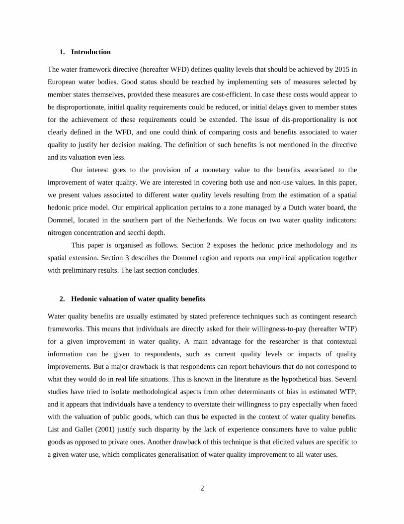
which are based on restricted versions of the SARAR(1, 1) model presented in equation (2). These
diagnostics are presented in Table 6.
Table 6 Spatial diagnostics on OLS residuals
Model 1 Model 2 Model 3 Model 4 Model 5 Model 6
LM Error model 665.9 390.2 897.8 563.2 577.4 916.9
LM Lag model 267.4 191.5 261.6 196.6 187.5 252.1
RLM Error model 543.4 310.1 763.1 469.5 485.1 784.0
RLM Lag model 145.0 111.3 126.8 102.9 95.3 119.1
Moran's I 0.0285 0.0219 0.0332 0.0263 0.0266 0.0335
Note: all test statistics are significant at the 1 percent level
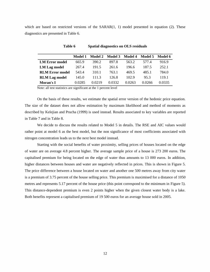
On the basis of these results, we estimate the spatial error version of the hedonic price equation.
The size of the dataset does not allow estimation by maximum likelihood and method of moments as
described by Kelejian and Prucha (1999) is used instead. Results associated to key variables are reported
in Table 7 and in Table 8.
We decide to discuss the results related to Model 5 in details. The RSE and AIC values would
rather point at model 6 as the best model, but the non significance of most coefficients associated with
nitrogen concentration leads us to the next best model instead.
Starting with the social benefits of water proximity, selling prices of houses located on the edge
of water are on average 4.8 percent higher. The average sample price of a house is 273 200 euros. The
capitalised premium for being located on the edge of water thus amounts to 13 000 euros. In addition,
higher distances between houses and water are negatively reflected in prices. This is shown in Figure 5.
The price difference between a house located on water and another one 500 metres away from city water
is a premium of 3.75 percent of the house selling price. This premium is maximised for a distance of 1050
metres and represents 5.17 percent of the house price (this point correspond to the minimum in Figure 5).
This distance-dependent premium is even 2 points higher when the given closest water body is a lake.
Both benefits represent a capitalised premium of 19 500 euros for an average house sold in 2005.
13
Table 7 Key estimation results (SEM, GM) – models 1 to 4
Model 1 Model 2 Model 3 Model 4
Edge of water 0.062***
0.062***
0.066***
0.066***
(0.02) (0.02) (0.02) (0.02)
Distance to river 0.000***
0.000***
(0.00) (0.00)
Distance to river (square) 0.000**
0.000***
(0.00) (0.00)
Distance to canal 0.000 0.000
(0.00) (0.00)
Distance to canal (square) 0.000 0.000
(0.00) (0.00)
Distance to swimming location 0.000 0.000
(0.00) (0.00)
Distance to swimming location (square) 0.000 0.000
(0.00) (0.00)
Proximity to river
0.004 0.010
(0.01) (0.01)
Proximity to a canal
0.027***
0.024***
(0.01) (0.01)
Proximity to a swimming location
0.012 0.013*
(0.01) (0.01)
Concentration in N 0.020***
0.023***
(0.01)
(0.01)
Concentration in N (square) 0.002***
0.003***
(0.00)
(0.00)
Concentration in N lower than 4
0.003
0.001
(0.01)
(0.01)
Concentration in N lower than 6
0.027**
0.031***
(0.01)
(0.01)
Concentration in N lower than 8
0.008
0.011
(0.01)
(0.01)
Concentration in N higher than 8
0.043**
0.044**
(0.02)
(0.02)
Secchi depth 0.004***
0.002* 0.004
*** 0.002
*
(0.00) (0.00) (0.00) (0.00)
Lambda 0.794***
0.761***
0.840***
0.805***
RSE 0.1633 0.1632 0.1633 0.1632
AIC 4080.0 4085.0 4082.0 4088.0
Standard errors in parentheses. Significance is indicated by *,
** and
*** for the 10, 5 and 1 percent level.

14
Table 8 Key estimation results (SEM, GM) – models 5 and 6
Model 5 Model 6
Edge of water 0.048**
0.048**
(0.02) (0.02)
Distance to any water 0.000***
0.000***
(0.00) (0.00)
Distance to any water (square) 0.000 0.000
(0.00) (0.00)
Closest water is a river 0.014 0.014
(0.01) (0.01)
Closest water is a canal 0.008 0.016
(0.03) (0.03)
Closest water is a lake 0.020***
0.018***
(0.01) (0.01)
Concentration in N 0.020***
(0.01)
Concentration in N (square) 0.002***
(0.00)
Concentration in N lower than 4
0.003
(0.01)
Concentration in N lower than 6
0.024**
(0.01)
Concentration in N lower than 8
0.004
(0.01)
Concentration in N higher than 8
0.044**
(0.02)
Secchi depth 0.004***
0.002
(0.00) (0.00)
Lambda 0.839***
0.803***
RSE 0.1631 0.1630
AIC 4092.0 4096.0
Standard errors in parentheses. Significance is indicated
by *,
** and
*** for the 10, 5 and 1 percent level.
We now turn to the discussion of coefficients associated with water quality indicators. Starting
with the turbidity indicator, an increase by 1 decimetre of visibility corresponds to an increase in house
price of 3.6 percent, which corresponds to a capitalised value of 995 euros. Given a discount rate of 4
percent, this corresponds to an annual premium of 40 euros per household.

15
Figure 5 Variation in house prices due to proximity to water
The variation in house price due to the concentration in nitrogen is non linear, and is presented in
Figure 6. The maximum house premium is reached for a nitrogen concentration of 4.2 mg/l, and amounts
to 4.3 percent of the house price, which corresponds to a capitalised value of 11 760 euros. Given a
discount rate of 4 percent, this corresponds to an annual premium of 470 euros per household.
Figure 6 Variation in house prices due to nitrogen concentration
4. Concluding remarks
The objective of this paper is to provide a monetary value to the benefits associated to improvements in
water quality. Our empirical application is based on the estimation of a spatial hedonic price model, with
a focus on two water quality indicators: nitrogen concentration and secchi depth. To our knowledge, this
was the first time the spatial structure of the data was accounted for in the context of the valuation of this
environmental good.
-0.06
-0.05
-0.04
-0.03
-0.02
-0.01
0.00
0 500 1000 1500 2000 2500
% c
han
ge in
ho
use
pri
ce
Distance to closest water body in metres
-0.080
-0.060
-0.040
-0.020
0.000
0.020
0.040
0.060
0 2 4 6 8 10 12
% c
han
ge in
ho
use
pri
ce
Concentration in N in mg/l
16
Our results are based on the estimation of a spatial error model by the generalised method of
moments. We find significant results for both visible (secchi depth) and invisible (nitrogen concentration)
water quality indicators. Based on our sample characteristics and given a discount rate of 4 percent, an
increase in secchi depth by 10 centimetres is associated to a yearly house premium of 40 euros per
household. Concerning nitrogen concentration, the premium is maximised for a concentration of 4.2 mg/l
and amounts to 470 euros per year per household. These results are net of additional benefits related to
the proximity to water, which represent a premium of 4.8 percent of the selling price when a house is
directly located on the edge of water. These benefits are complemented by distance-based premiums
which also depend on the type of water body closest to a dwelling.
In a next step, we will extend the time scale of the empirical application in order to investigate the
impact on house prices of actual changes in water quality. In addition, we will place more efforts on the
relation between our two water quality indicators and the WFD requirements. A final step then will be to
compare the benefits of achieving these requirements to the costs of measures needed to be implemented.
We currently investigate these costs in a parallel research project.

17
References
Anselin L. (1988). Spatial econometrics: Methods and models. Kluwer, Dordrecht.
Anselin L. (2006). Spatial Econometrics. In: Palgrave handbook of econometrics: Volume 1, Econometric
theory (ed. Mills and Patterson). Basingstoke, Palgrave Macmillan, pp. 901-969.
Anselin L. & Lozano-Gracia N. (2008). Errors in variables and spatial effects in hedonic house price
models of ambient air quality. Empirical Economics, 34, 5-34.
Bin O., Crawford T.W., Kruse J.B. & Landry C.E. (2008a). Viewscapes and Flood Hazard: Coastal
housing market response to amenities and risk. Land Economics, 84, 434-448.
Bin O., Kruse J.B. & Landry C.E. (2008b). Flood hazards, insurance rates, and amenities: Evidence from
the coastal housing market. Journal of Risk and Insurance, 75, 63-82.
Boyle K.J., Poor P.J. & Taylor L.O. (1999). Estimating the demand for protecting freshwater lakes from
eutrophication. American Journal of Agricultural Economics, 81, 1118-1122.
Brasington D.M. & Hite D. (2005). Demand for environmental quality: a spatial hedonic analysis.
Regional Science and Urban Economics, 35, 57-82.
Brouwer R., Hess S., Wagtendonk A. & Dekkers J. (2007). De Baten van Wonen aan Water: Een
Hedonische Prijsstudie naar de Relatie tussen Huizenprijzen, Watertypen en Waterkwaliteit. In.
Daniel V.E., Florax R.J.G.M. & Rietveld P. (2007). Long term divergence between ex-ante and ex-post
hedonic prices of the Meuse River flooding in The Netherlands. In: (ed. Working Paper - ERSA
conference 2007).
Daniel V.E., Florax R.J.G.M. & Rietveld P. (2009). Flooding Risk and Housing Values: An Economic
Assessment of Environmental Hazard. Ecological Economics, 69, 355-365.
Epp D.J. & AlAni K.S. (1979). The effect of water quality on rural nonfarm residential property values.
American Journal of Agricultural Economics, 61, 529-534.
Gawande K. & Jenkins-Smith H. (2001). Nuclear waste transport and residential property values:
Estimating the effects of perceived risks. Journal of Environmental Economics and Management, 42,
207-233.
Gibbs J.P., Halstead J.M., Boyle K.J. & Huang J.C. (2002). An hedonic analysis of the effects of lake
water clarity on New Hampshire Lakefront properties. Agricultural Resource Economic Review, 31, 39-
46.
Kelejian H.H. & Prucha I.R. (1999). A generalized moments estimator for the autoregressive parameter in
a spatial model. International Economic Review, 40, 509-533.
Kim C.W., Phipps T.T. & Anselin L. (2003). Measuring the benefits of air quality improvement: a spatial
hedonic approach. Journal of Environmental Economics and Management, 45, 24-39.
Leggett C.G. & Bockstael N.E. (2000). Evidence of the effects of water quality on residential land prices.
Journal of Environmental Economics and Management, 39, 121-144.
List J.A. & Gallet C.A. (2001). What experimental protocol influence disparities between actual and
hypothetical stated values? Environmental & Resource Economics, 20, 241-254.
Poor P.J., Pessagno K.L. & Paul R.W. (2007). Exploring the hedonic value of ambient water quality: A
local watershed-based study. Ecological Economics, 60, 797-806.
Rosen S. (1974). Hedonic Prices and Implicit Markets - Product Differentiation in Pure Competition.
Journal of Political Economy, 82, 34-55.
Steinnes D.N. (1992). Measuring the Economic Value of Water-Quality - the Case of Lakeshore Land.
Annals of Regional Science, 26, 171-176.

18
Appendix 1 Summary statistics
Continuous variables
Minimum Maximum Mean
Price 22000 2950000 273204
Surface (square metres. log) 3.69 6.2 4.9
Number of rooms 0 15.0 4.9
Number of bath-rooms 0 8.0 1.0
Index of maintenance 1 9.0 7.0
Index of insulation 0 5.0 1.7
Proportion of foreigners 1 40.0 7.2
Average income per inhabitant 81 186.0 111.7
Proportion of non-active 4 51.0 15.9
Index for water richness 0 44.2 3.7
Distance to the river 25 3795 990.2
Distance to a lake 16 4482 683.5
Distance to a canal 95 18602 3586.7
Distance t a swimming location 215 11808 2867.1
Distance to a city water 10 6548 390.4
Concentration in N 0.6 8.8 2.7
Secchi depth in decimetres 0 15.7 7.6
Categorical variables
Sum
Uden 110
Den Bosch, Waalwijk Drunen 601
Breda, Tilburg 1510
South East Brabant 345
Built before 1905 126
Built between 1991 and 200 668
Built after 2001 101
Townhouse 2400
House in a row 161
Corner house 939
Half of a dubble house 1082

19
Simple house 141
Single-family house 4089
Manor house 649
Farm house 220
Villa 185
Practice possible 212
Practice present 148
Parking lot 90
Carport 205
Garage 1602
Both carport and garage 113
Garage adapted to several cars 275
Gas or coal heating 127
Central heating boiler 5091
First sale (no public notary charges) 16
Ground rent 6
Urbanisation > = 2500 addresses per km2 1088
Urbanisation 1500 - < 2500 addresses per km2 1039
Urbanisation 500 - < 1000 addresses per km2 1501
Urbanisation < 500 addresses per km2 283
Garden towards South 1674
Residential area 4035
City center 379
Edge of a wood 117
Edge of water 56
Edge of a park 214
Unobstructed view 545
Busy road 248