RASMUS UNIV RSITY ROTT R AM Thesis Marin... · Emami Namini and his feedback and advice on my work....

1

ERASMUS UNIVERSITY ROTTERDAM

Master Thesis

Corruption and Growth, an Empirical Study of 40

European Countries

Marin Marinov

324355

Thesis Supervisor: Professor Dr. Benoit Crutzen

Second Reader: Professor Dr. Julian Emami Namini

2

Table of Contents

Acknowledgement........................................................................................... 3

Abstract .......................................................................................................... 4

I. Introduction .............................................................................................. 5

II. The two views on corruption ..................................................................... 8

III. Theoretic Framework ........................................................................... 12

IV. Data ..................................................................................................... 14

1. Data Description .................................................................................. 14

2. Comparative Statistics of the data ....................................................... 19

V. Methodology ........................................................................................... 24

VI. Results ................................................................................................. 27

1. Short-run Scenario ............................................................................... 27

2. Long-run Scenario ................................................................................ 35

VII. Limitations and Further Research ......................................................... 42

VIII. Conclusions .......................................................................................... 43

Bibliography .................................................................................................. 45

Appendix ....................................................................................................... 45

Panel Data: ................................................................................................... 49

3

Acknowledgement

It is with great gratitude that I would like to acknowledge the support and patience of my supervisor

Professor Dr. Benoît Crutzen. His guidance and suggestions have helped me immensely in finishing

my thesis in a way I can be proud of. Without his quick responses to my questions and feedback to

my research, completing this thesis would not have been possible. Thank you Professor Crutzen!

Next I would like to express my gratitude towards the second reader of my thesis, Professor Dr. Julian

Emami Namini and his feedback and advice on my work. I would also like to thank Ivan Lyubimov

from the Erasmus School of Economics, a PhD Candidate, who volunteered his time and efforts to

help me understand better the theoretical aspects of my thesis and their implications. Our Skype

conversations also played a key inspirational role in finishing my thesis. Additionally, I would like to

thank all the teachers and professors throughout my Masters and Bachelors who gave me the

knowledge and tools in order to handle the daunting task of this thesis.

I would like to thank my parents for their support and the opportunity they have given me to study in

an elite international university. And finally, I would like to acknowledge my friends who have spent

many nights debating with me on the topic of this thesis and inspiring me to finish it in the way I

have.

4

Abstract

This thesis empirically investigates the relationship between corruption and growth of GDP per capita

in real terms. There are two opposing views on the nature of the effects of corruption, some calling it

“the helping hand” (Leff, 1964), while others - “the grabbing hand” (Mauro, 1995). This paper

composes a dataset of 40 European countries for the time period 1998-2011 with the goal of

analyzing the exact nature of the relationship. Both the short-run and the long-run are analyzed

through a panel and a cross-section study, respectively. The empirical analysis in the short-run isn’t

successful in confirming a significant link between growth and corruption thus does not disprove

either of the views on corruption. However, in the long-run cross-section regressions the findings

indicate a very strong and significant negative relationship between the two. This confirms the

“grabbing” effect of bribery on a county’s economy in the long-run.

5

I. Introduction

The effect of corruption on economic growth has been a long and heated debate in the economic

community. Data from Transparency International in recent years indicates that corruption has been

“rampant” in over 70 countries, including some of the world’s most populous and fastest growing

economies such as China and India, countries that account for a large and rapidly increasing share of

the global economy. However, the exact effects that corruption has on growth still remain unclear.

Some have argued that bribes perhaps act as a piece-rate wage for bureaucrats who generally tend

to be under-paid and thus under-motivated to do their job efficiently. Thus administrative corruption

is an effective tool for cutting through excess red-tape and helps speed up the wealth-generating

activities of firms. On the other side of the economic spectrum, some believe that corruption is

damaging for innovation and investments and thus for growth. This view has been spearheaded in

recent years by Paolo Mauro with his famous paper from 1995, "Corruption and Growth". Whatever

stance one takes on the topic, corruption remains as one of the main issues and concerns of every

government and society on the globe and thus presents itself as a fascinating research topic. In this

paper I will first review both points of view on the effects on growth and then follow the analysis of

previous researchers with my own empirical study on a data-sample I have gathered consisting of

subjective indices, growth variables and GDP for 40 European countries in the period between 1998

and 2011. But before we begin with the literature review and empirical research, let us first

introduce the topic in more detail.

What is corruption to begin with? And while it has many names – bribery, kickback, or in the Middle-

East – baksheesh, how do we define it so that we can determine its effects? Over the course of time,

corruption has gathered a wide myriad of definitions. They vary and often confuse, therefore in this

paper I will attempt to define a narrow and clear meaning for the term. Where does the word derive

from? The roots of corruption come from the Latin adjective corruptus, meaning spoiled, broken or

destroyed. Those who turn to the Oxford Advanced Dictionary will find the following – “dishonest or

illegal behavior, especially of people in authority:” The Concise Oxford English Dictionary is more

precise in its definition, describing the word in its social context as bribing - an act of “moral

deterioration”. The Merriam Webster’s Collegiate Dictionary defines corruption as “inducement to

wrong by improper or unlawful means (as bribery).”

What does the economic literature have to say about corruption and its definition? In his work from

1996, “The search for definitions: the vitality of politics and the issue of corruption”, Johnston

provides an important typology for the definition of corruption. The author divides the existing

6

literature into two separate groups. The first group, which he associates with the works of Friedrich

1966, Nye, 1967, Van Klaveren, 1989 and Heidenheimer, 1989, has its focus on the behavioral

aspects of corruption. To Johnston, these behavior-focused works all share the opinion that

corruption is the abuse of public office, power or authority in the aim of achieving private gain. Nye

(1967) defines it as “behavior which deviates from the formal duties of a public role because of

private-regarding (personal, close family, private clique) pecuniary or status gains; or violates rules

against the exercise of certain types of private-regarding influence”. Even though not mentioned in

the work of Johnston (1996), Garner (2004:370) also gives a definition consistent with this first

group. He defines corruption as “The act of doing something with an intent to give some advantage

inconsistent with official duty and the rights of others, a fiduciary’s official’s use of a station or office

to procure some benefit either personally or for someone else contrary to the rights of others”.

The second group of researchers, according to Johnston, defines corruption by focusing on the

principal-client-agent relationship. Among the representatives of this group, the author mentions the

works of Rose-Akerman, 1978; Klitgaard, 1988 and Alam, 1989. To him, these researches focus more

attention to the interactions between and among the involved parties of the above-mentioned

relationship. In his work, Alam defines corruption as “… (1) the sacrifice of the principal’s interest for

the agent’s, or (2) the violation of norms defending the agent’s behavior”.

So far, the definition given by the two groups can be summarized as follows. The first one seems to

focus on corruption as a phenomenon that exists in the public sector. The second groups of

definitions escape the apparent weakness of the previous ones, by not confining corruption only to

the public sector. However, when one includes the private sector in the equation as well, he risks

defining corruption too broadly and making any empirical research on the matter highly complex. It

is for this reason that in this paper I will adopt a definition that confines my research only on the

corruption in the public sector. Therefore, I define corruption as follows: “the abuse or complicity in

abuse of public power, office or resources for the goal of achieving personal gains”.

Although there has been a lot of attention on the issue of corruption on both an international level,

mainly by campaigns from the United Nations and the World Bank, and on a national level, the

presence of corruption in the public sector as it is perceived by the population doesn’t cease to grow.

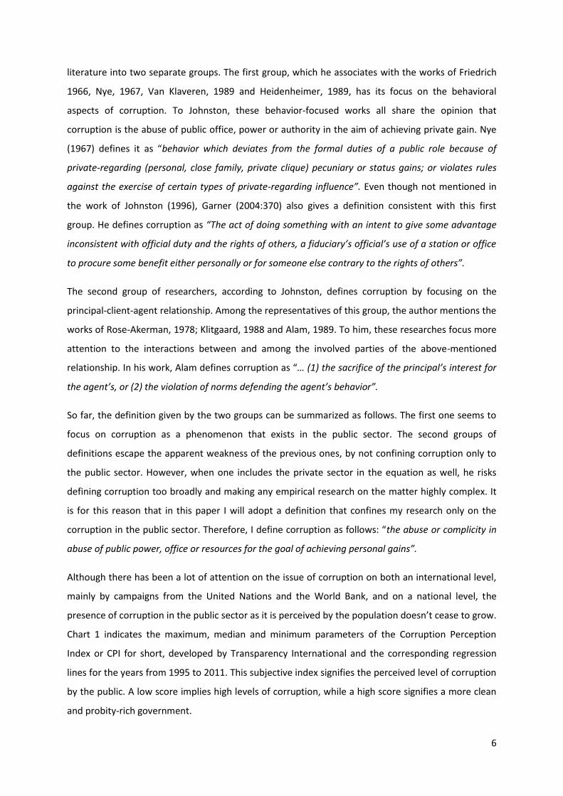
Chart 1 indicates the maximum, median and minimum parameters of the Corruption Perception

Index or CPI for short, developed by Transparency International and the corresponding regression

lines for the years from 1995 to 2011. This subjective index signifies the perceived level of corruption

by the public. A low score implies high levels of corruption, while a high score signifies a more clean

and probity-rich government.

7

Chart 1

What Chart 1 shows is that the distribution has shifted to its lower end of the scale. All parameters

exhibit decay in the public sector. This occurs not only in the most corrupt nations, but affects the

less corrupt as well. The shift is strongest in the median. Here one can observe an average annual

change rate of -3.4% (the regression line slope is -0.13). This signifies a deterioration of social morals

in more than half of the countries the CPI index covers in its research. This longer term trend is

worrisome and merits further investigation into the effects the corruption phenomenon has on the

world economy. Although this is hardly the first paper to investigate the link between corruption and

growth (Leff, 1964; Huntington, 1968; Acemoglu and Verdier, 1998; all suggest corruption might be

desirable for economic growth, while Gould and Amaro-Reyes, 1983; Murphy et al, 1993; Mauro,

1995; Mo, 2001 and most recently, Aidt, 2009 - claim that corruption damages investment and

innovation and therefore is detrimental for growth), most of the works done on the subject use older

datasets for a wide myriad of countries from all continents. Even one of the most recent works by

Aidt, 2009 uses dataset that is only up to the year 2000. I will provide a more recent data-sample I

have combined from indices, growth variables and GDP for 40 European countries for the period

8

from 1998 to 2011. The data I have collected has come mainly from the sources of Transparency

International, the World Bank, Penn World Tables and Barro-Lee’s data sample on Schooling.

The main hypothesis I will be testing is if there is a link between economic growth (in real terms) and

corruption in the economies of Europe and if such a link exists, is its effect negative or positive. The

Null Hypothesis I will be testing is that there is no significant link between the two. I will do this by

looking at the link between corruption (expressed by the CPI Index from Transparency International)

and growth of real GDP per capita. I will use first a paneI study to check for first the short-term

relationship between the two and then a cross-sectional regression to check for the medium/long-

term effects. What I expect to find is a significant negative relation between the level of corruption

and growth of GDP in real terms, with the relationship being stronger and more significant in the

medium/long-run scenario. (Although, since the CPI Index measures corruption with 1 being the

most corrupt and 10 the least corrupt, statistically the relation should be positive between the values

of CPI and RealGDP per capita).

In the next section, I will take a closer look at the debate on whether corruption helps grease the

cogs of the economy and stimulates growth or does it damage the growth of GDP. After that, I will

present the theoretical framework and the model I will use, followed by a section devoted to the

methodology used in this paper. Next, I will present a section that takes a deeper focus on the

dataset I have constructed and used to test the effects of corruption, explaining how the data was

gathered, why I have chosen the 1998-2011 time-frame, why I have chosen the 40 European

countries and some descriptive statistics about the data itself. Finally, I will analyze the results of the

empirical research and draw conclusions based on them.

II. The two views on corruption

While all economists undoubtedly agree corruption has a significant effect on investments and

growth, there are discerning views on what the net effect is. As Aidt (2009) puts it, the world is

populated by two types of people – the “sanders” and the “greasers”. The sanders are those who

believe that bribes and other acts of corruption “sand”, that is hinder, development, while the

greasers hold the view that, in some cases, corruption can grease the cogs of the economic machine

and thus help foster growth. Perhaps the best example of a “greaser” paper is the classic work by

Nathan Leff – “Economic Development through Bureaucratic Corruption” from 1964. While the view

that corruption can be beneficial for commerce wasn’t new at the time of Leff’s work, his paper

9

helped it gain prominence. The paper’s significance nowadays should not be underestimated as it has

been used as a theoretic basis for more recent works such as Lui (1985) and Beck and Maher (1986).

Further claims that support its results have come from empirical papers such as the one of Egger and

Winner from 2005. They conclude that “using a data set of 73 developed and less developed

countries, we find that corruption is a stimulus for FDI, which confirms the position of Leff (1964)

that corruption can be beneficial in circumventing regulatory and administrative restrictions”. What

is the general idea behind the view of Leff and other researchers that see corruption as the grease

necessary to run the commerce machine at full speed? The first thing Leff does to defend his position

is to distinguish between bureaucratic corruption and bureaucratic inefficiency. “Corruption refers to

extra-legal influence on policy formulation or implementation. Inefficiency, on the other hand, has to

do with success or failure in attaining given goals, whether those of its political directors, or those of

the grafters.” (Leff, 1964). Leff strongly believes that corruption can have a positive effect in

economies that suffer from government and administrative inefficiencies, since corruption facilitates

beneficial transactions that would otherwise not have occurred and thus corrects the shortcomings

of the administration. According to him, this is especially the case in underdeveloped countries,

where the government might have other priorities and the importance of economic development is

only given lip-service. In such cases, the bureaucracy and authorities generally are more concerned

with maintaining the status-quo and could even dislike the emergence of a competing center of

power, such as a strong and wealthy middle-class. Through graft, entrepreneurs can induce the

administration to take a more favorable stance on activities that would help foster economic growth.

Graft can also motivate the bureaucracy to be more efficient in its task of allocating resources to the

most productive of the entrepreneurs. According to Leff, this is done by allowing individuals in the

private sector to outbid each other for the allocation of scarce licenses or favors and with

competition driving prices upwards, the licenses and favors will tend to go to those who can pay the

highest prices. In the long run, this will make sure that the favors will go only to the most efficient

producers, as they will be able to out-bid less competitive peers. To Leff, this is a situation where the

efficient out-do the inefficient and thus presents itself as a good self-correcting mechanism for the

market. The author sets the following example to illustrate his theory. In the early 1960s, the

government agencies of Chile and Brazil were given the job to enforce price controls for food

products. In Chile, the administration strictly enforced the freeze as was charged to do. That resulted

in a stagnation of food production. In contrast to Chile, the Brazilian agencies were corrupt and

sabotaged the freeze, resulting in a substantial increase in food production.

Daniel Levy provides another example from the real world in his work from 2007 - Price adjustment

under the table: Evidence on efficiency-enhancing corruption – that supports the claims of the

10

greasing effect of corruption. Based on his first-hand experience, his paper offers anecdotal evidence

on price-setting and price-adjustment mechanisms that were in usage in the Republic of Georgia

during the Soviet planning and rationing regime (1960-1971). In his work, Levy depicts the creative

and sophisticated ways that were used to deal with the artificially created shortages of the inefficient

central-planned economy of the Soviet Union and its distorted relative prices. Rent-seeking behavior

led to the allocation of significant real resources for the development and maintenance of an

unexpectedly efficient and well-functioning chain of black markets. This was done through a chain of

bribes and secret payments which resulted in the fact that the Georgian economy could produce far

more output and allocate it far more efficiently than would have otherwise been feasible.

Next on I will present the paper of Peter Egger and Hannes Winner – Evidence on corruption as an

incentive for foreign direct investment. The reason why I have chosen this paper in particular out of

all the ones defending the positive externalities of corruption is because it assesses the relationship

between corruption and inward foreign direct investments (FDI), an aspect I will examine in detail in

the empirical part of my paper and its focus on distinguishing between the long and short term

influences of perceived corruption. Egger and Winner use a sample of 73 developed and less

developed countries for the time period 1995-1999 and find a clear positive relationship between

corruption and FDI and thus conclude corruption is a stimulus for FDI, thus confirming the

proposition of Leff (1964). How do they come to that conclusion? Prior research done before their

paper, mainly analyzing cross-section data => therefore focusing on the long run, tends to find a

negative long run impact of corruption on FDI. The Co-authors thus decide to assess the short and

long run impact of corruption on inward FDI stocks by using a panel study to see if there is any

significant difference between the two. To accomplish this, they disentangle the short run from the

long run by estimating a Hausman-Taylor model and thus accounting for the potential endogenity of

the long run. What is more fascinating in this paper is the results Egger and Winner find on the

internal distributional effect of corruption on FDI. Their findings suggest that the long run

contribution of the perceived corruption amounts to up to 40%, while the short run contribution is

5% of the observed overall FDI growth in their sample of countries in the 1995-1999 period.

Furthermore, the observed change in corruption has accounted for an equalization effect on the

international distribution of real inward FDI shares (though only accounting 1% for a long run

increase in the entropy index).

What do the “sanders” have to say about all this? It seems the “helping hand” theory has no lack of

evidence supporting its case, but is corruption all that good? Perhaps it can be circumstantially

beneficial only in the cases of major administrative or government failures? Mauro (1995) explores

that probability by measuring the effects of the indices for corruption, red tape, the efficiency of the

11

judicial system and various categories of political stability on the growth of the economy of a cross

section of countries. To him, the interaction between the institutions and economic growth is two-

sided. While institutions undoubtedly affect economic variables and performance, at the same time,

the same economic variables may affect the institutions themselves. In order to escape the issue of

endogenity, Mauro uses an index of ethno-linguistic fractionalization (an index that measures the

probability that two persons drawn at random from a country’s population will not belong to the

same ethno-linguistic group) as an instrument in his regressions. What he finds contradicts with the

position of Leff (1964) and directly that of Egger and Winner (2005). Mauro finds that corruption

lowers private investment and thereby, reduces economic growth even for a subsample of countries

where government and bureaucratic regulations and red tape are very cumbersome and major

administrative failures are present. His results are significant both statistically and economically.

Mauro (1995) gives an example of his findings. He suggests that if Bangladesh were to increase the

integrity and efficiency of its administration by one standard deviation increase in the bureaucracy

efficiency index, its investments rate would increase by 5 percent, which in turn, would result in an

increase in the annual GDP growth increase by half a percentage point. He concludes that

bureaucratic efficiency is perhaps just as important determinant of investments and thus growth, as

is political stability and thus puts support to the theory of corruption’s “grabbing hand” effect.

Another interesting “sander” paper is the 2001 work of Pak Hung Mo – “Corruption and Economic

Growth”. Similarly to Mauro (1995), Mo does an empirical study in order to provide quantitative

estimates on the impact of corruption on the growth of an economy. Unlike previous literature,

however, Mo explores the importance of the transmission channels through which corruption affects

investment and growth. The author presents the three most important to him, of these channels –

the Investment channel, the Human Capital channel and the Political Stability channel. His results are

consistent with Mauro (1995). He finds that a one-unit increase in the corruption index (the

perceived corruption index CPI) reduces the growth rate of an economy by 0.545 percentage points.

While corruption lowers growth through all 3 of the channels he differentiates, its strongest effect is

via the Political Stability one, which accounts for around 53% of the overall effect. Additionally, he

finds that corruption is most prevalent in countries where other forms of institutional inefficiencies

and administrative failures are present, such as bureaucratic red tape and weak or inefficient

legislative and judicial systems. Mo concludes that perhaps all these effects are perhaps a

manifestation of a single phenomenon and thus should be considered as a whole.

Aidt (2009) takes a slightly different approach then Mauro (1995) and Mo (2001) before him. In his

paper “Corruption, institutions and economic development” he looks at the relationship between

growth in genuine wealth per capita, a direct measure, the author believes, of sustainable

12

development, and corruption. Aidt describes corruption as a source of short-term unsustainable

growth and while circumstantially an effective lubricator that speeds up the entrepreneurs’ wealth

generating activities, in a broader sense, corruption is an obstacle for long-term sustainable

development. One of the main arguments he puts is the logical fallacy of efficient corruption. If a

bureaucrat, who is interested in rent-seeking, knows corruption is a useful tool to overcome

cumbersome procedures and excessive red tape or other administrative inefficiencies, he has an

incentive to create and maintain such administrative inefficiencies precisely because of their

corruption potential. This will cause substantial amounts of real resources to be devoted to

contesting the associated rents. The result will be pure waste and misallocation of resources. Even if

there are singular examples of efficiency-enhancing corruption on a microeconomic level, according

to Aidt, they should not be taken as evidence of the same effect on a macroeconomic level. From a

quantitative point of view, unlike the works of Mauro and Mo, the paper is unsuccessful in its

attempt at producing statistically robust and convincing evidence of the negative link between

corruption and GDP per capita. However, Aidt does present quantitative evidence in the form of field

studies and survey points to the substantial cost of corruption. Even though Aidt may not have

proven the link statistically, his work does indicate that corruption is a hindrance to sustainable

growth. His theoretic model and theoretic framework provide a very interesting and clear

explanation on the possible mechanism that makes corruption an ineffective tool for dealing with

bureaucratic inefficiency and failures, as well as fostering sustainable growth. The insight his paper

provides is the reason why I will use it as my own theoretic framework.

III. Theoretic Framework

After analyzing some of the most prominent works on the subject of corruption and growth,

discussing the views of both “greasers” and “sanders”, I will now continue this paper with a theoretic

framework in order to explain why I believe a link exists between corruption and growth and why I

believe the relationship is a negative one. As I said above, the model I will present is a theoretic

model based of the insights of Aidt (2009) about the efficient corruption logical fallacy. We have seen

so far that corruption is indeed more evident in an economy suffering from administrative failures

and or bureaucratic inefficiency. So let us assume first an economy without government

intervention, a perfectly competitive market. This economy consists of a continuum of agents. Each

of these agents can become an entrepreneur or works for a wage. Each of these agents is

differentiated by their level of entrepreneurial skills and productivity or to say it in another way, their

13

comparative advantage. In this model, we will call this comparative advantage “a” with a being

uniformly distributed between [0, 1]. a = 1 will present the most skilled and productive

entrepreneurs while a = 0 the least skilled and productive. If an agent decides to work as a worker in

the private sector, his wage will be w, with w not changing regardless of his entrepreneurial skills and

productivity a. The wage will, however, increase with the number of firms n. Additionally, the profits

of the entrepreneur decrease with the increase in n. An agent becomes an entrepreneur if

. If an entrepreneur’s comparative advantage is high, he is able to produce more

cheaply and efficiently, this retaining a higher percentage of the value he produces. In an economy

without government intervention, individuals with high levels of a create firms until the profit from

the two employment opportunities is the same -> This result is market

efficient and allocatively efficient, therefore government intervention isn’t necessary or warranted.

Yet suppose that the administration decides to implement licenses in order for an entrepreneur to

set up a firm and begin wealth generating activities. If the number of licenses, let us denote them as

λ, is equal to the number of firms in market equilibrium , nothing changes in the economy. The

market is still in equilibrium and resources are allocated efficiently. Now assume, however, that λ is

smaller than . In this case, the government must decide on how to distribute the licenses among

the entrepreneurs who want to set up their operations. Since the administration cannot observe the

comparative advantage a of each entrepreneur, they have to either distribute the licenses at random

or sell them to the highest bidder. In the first scenario, the government distributes the licenses at

random which might cause some entrepreneurs with a low value of a to set up firms and thus cause

a misallocation of resources. The latter option, where a corrupt government official sells the licenses

to the highest bidder at first seems like a more effective way for allocation, as only agents with the

highest value of a would compete for the licenses. In this sense, here corruption can be seen as

efficiency-enhancing as more output will be produced than in the non-corrupt case. This is similar to

the examples of Leff (1964) of the food production freeze in Brazil and Chile. This scenario creates

some complications however. First, it would be far more efficiently-enhancing for the government to

not intervene at all or to set the number of licenses λ equal to . Since we assume all agents to be

perfectly rational and the bureaucrats to be the ones determining the number of licenses in the

economy λ, they have no incentive to set the number of licenses λ equal to the equilibrium number

of firms , as in that way they do not generate additional income. The profits of the public sector

agent will increase from = t to = t+c, in the corruption scenario, with c representing the scarcity

rent the bureaucrat will gain from selling the licenses and t being the wage of the bureaucrat. In fact,

we expect the bureaucrat to set the number of licenses λ, in a way to maximize the value of c or the

profits they will gain from corruption. This will definitely mean setting the number of licenses λ

14

below the optimum. What this argument says is that not only does corruption not help in cases of

government failures and bureaucracy inefficiencies, in fact, knowing that those inefficiency have

corruption potential, the administration would purposely impose and maintain them in order to

generate rent from the entrepreneurs. This scenario creates misallocation of resources, as agents

with high comparative advantage are now interested in private sector jobs. Since fewer

entrepreneurs will produce in this equilibrium than in the perfectly competitive market one,

investments will decrease and the overall output of the economy will suffer a decrease as well and in

this way, decreasing the overall growth of the economy. The crucial point of this model, similar to the

insight of Aidt (2009), is that corruption and bureaucratic inefficiency are two elements of the same

phenomenon, undividably linked together. Inefficient regulations generate scarcity rents and those

scarcity rents by themselves create corruption potential as individuals are only willing to pay to

obtain licenses if they are scarce. And even if, as some of the “greaser” papers suggest, corruption is

a useful tool to circumvent cumbersome regulation or bureaucratic inefficiencies in the short-run, it

provides enough incentives for the creation of more such regulation and inefficiencies in the long-

run. In the empirical analysis, we would expect that an increase in the Gastil index (that is, worsening

of the political freedom and bureaucratic efficiency) and a decrease in the corruption perception

index CPI (that is, an increase in the perceived corruption in the public sector) to have negative

effects on investments and the growth of real GDP per capita. Since the effects of change in

corruption and administrative efficiency take time to bear fruit, we would expect the impact on GDP

growth and investments to be more pronounced in the long-run than in the short-run.

IV. Data

1. Data Description

For the purpose of testing empirically the main hypothesis of whether a link between corruption and

growth exists, I have constructed a data-sample taken from 40 European countries for the time

period from 1998 to 2011. The main reason I have done so is because previous papers that have

been written on the topic of corruption and growth all use older data-series, with even the most

recent ones using samples going only until the year 2000. Therefore, in order to see if the results of

previous researchers are consistent with more recent data, I have collected a data-sample, consisting

of subjective indices, growth variables and real GDP per capita from Transparency International, The

World Bank, Penn World Tables and The Barro-Lee sources on schooling for the countries: Albania,

Austria, Belarus, Belgium, Bosnia and Herzegovina, Bulgaria, Croatia, Cyprus, The Czech Republic,

15

Denmark, Estonia, Finland, France, Germany, Greece, Hungary, Ireland, Italy, Latvia, Lithuania,

Luxembourg, Former Yugoslavian Republic of Macedonia, Malta, Moldova, Montenegro, (for the

years 1998 and 1999, I used data for Serbia for the CPI and Gastil Indexes) The Netherlands, Norway,

Poland, Portugal, Romania, Russia, Serbia, Slovakia, Slovenia, Spain, Sweden, Switzerland, Turkey,

Ukraine and the United Kingdom. Initially, the data set also included Monaco, Kosovo, Lichtenstein,

San Marino, the Vatican and Andorra, Armenia, Georgia, Iceland but they were dropped from the

series due to insufficient data. (Transparency International did not include most of these countries in

its CPI Index until much later on in the series). Why have I chosen only European countries? In

previous works, the data sample has always had a diverse selection of developed and developing

countries from all around the globe. Representatives of almost every continent were present in the

data-series. The reason I chose to focus my attention only on Europe is because, even though

European countries differ substantially between each other (for example, the Netherlands are very

different culturally, ethnically and linguistically from Russia, yet Russia is much more similar to the

Netherlands, when compared to China), they still share more commonalities then differences. In that

way, I account to some extent for cultural effects on corruption.

Another reason why I have limited my research to Europe only is the fact the continent provides us

with an excellent sample of countries, distributed along the whole spectrum of parameters. In terms

of the level of CPI, Europe has the 2 highest ranking countries in the index, Denmark and Finland,

which have scored on more than one occasion the perfect score of 10. On the other hand, the

European series also includes examples such as Albania, Serbia and Russia with scores comparable to

third-world countries in Africa in terms of corruption. This diversity and distribution of countries in

the data I hope will provide my empirical research with good and robust results on the link between

corruption and growth.

The main indicator I am using in this paper for measuring corruption is the Corruption Perception

Index which ranks countries according to their perceived level of public-sector corruption. This index

is consistent with my definition of corruption as - “the abuse or complicity in abuse of public power,

office or resources for the goal of achieving personal gains” – since it limits the scope of research to

only the public sector. The index ranks its scores from 1 to 10. A score of 10 signifies that the county

is a paragon of probity and there is no perceivable corruption, while a score of 1 shows that

corruption dominates the country entirely. The index itself is a composite index, drawing on

corruption related data by a variety of independent and reputable institutions. The main reason the

researchers at Transparency International use an aggregate index of individual sources, rather than

taking each score separately, is that a combination of sources measuring the same phenomenon is

much more reliable and robust. To be included in their CPI index, a source must measure the overall

16

extent of corruption (frequency and/or size of corrupt transactions) in the public and political sectors

and measure perceptions of corruption in at least a few different countries. The methodology used

to assess the perception has to be the same for all assessed countries. There are two different type

of sources included in the CPI Index. The first one is business people opinion surveys on how much

corruption influences their activities. The second one is assessment scores of a country’s

performance, provided by a group of country/risk/expert analysts. (For example, the 2009 CPI

includes 6 assessments of business people surveys: IMD 2008 and 2009, PERC 2008 and 2009 and

WEF 2008 and 2009. The other 7 sources used in the construction of the index are assessments

provided by country experts or analysts). Since each of the sources uses its own scaling system, the

researchers at Transparency International standardize the data before entering it into the index (For

details on how this is achieved refer to www.Transparency.org/cpi).

The next index I use in the data is the Gastil measure of world freedom, taken from the annual report

prepared by the Freedom House on World Freedom (Since 1989 the survey has been renamed to the

Freedom of the World, however, it used to be called the Gastil index in honor of Raymond Gastil, a

Harvard-trained specialist in regional studies who developed the survey’s methodology in 1972). I

calculate the Gastil Measure by taking the scores of political rights and civil liberties per country,

presented in the report, adding them together and then dividing by 2. The survey used in the report

provides an annual evaluation of the state of global freedom as experienced by individuals. The

ratings are divided into 2 categories – Political rights and civil liberties. Political rights enable people

to participate freely in the political process, including the right to vote freely, compete for public

office, join political parties and organizations and elect representatives who have a decisive impact

on public policies. Civil liberties on the other hand allow for freedoms of expression and belief

associational and organizational rights, rule of law, personal autonomy without interference from the

state and etc. The survey does not rate governments and or government performance per se, what it

does measure is the real-world rights and social freedoms of individuals. The survey tries to reflect

the interplay between a variety of governmental and non-governmental actions that affect the

freedoms. An important note on the survey is that the Freedom house does not maintain a culture-

restricted view of freedom, but grounds its methodology in basic standards of rights and liberties,

derived from the Universal Declaration of Human Rights. The ratings are done on a scale of 1 to 7,

with 1 indicating the highest degree of freedom and 7 – the lowest. These ratings are applied to 192

countries around the globe. (for a more detailed look at the methodology of the report, please visit

http://www.freedomhouse.org/report/freedom-world-2010/methodology).

Next I will present the growth variables I have assembled for the data sample of the 40 countries in

the 1998-2011 period. The variables come from the data banks of the World Bank, The Penn World

17

Tables and The Barro-Lee data sample on Schooling. The values for foreign direct investment (FDI)

were gathered from the World Development Indicators (WDI), the primary World Bank databank,

compiled from official-recognized sources of development data of national, regional and global

estimates. Foreign direct investment are the net inflows of investment to acquire a lasting

management interest (10 percent or more of voting stock) in an enterprise operating in an economy

other than that of the investor. It is the sum of equity capital, reinvestment of earnings, other long-

term capital, and short-term capital as shown in the balance of payments. This series shows net

inflows (new investment inflows less disinvestment) in the reporting economy from foreign

investors. Data are in current U.S. dollars.

Initial GDP, converted using PPP, from the year 1998 has been taken from the Penn World Tables

database. PPP GDP is gross domestic product converted to international dollars using purchasing

power parity rates. An international dollar has the same purchasing power over GDP as the U.S.

dollar has in the United States. Data are in constant 2005 international dollars. The growth indicator I

have chosen is GDP per capita based on purchasing power parity (PPP). PPP GDP is calculated as

gross domestic product converted to international dollars using purchasing power parity rates. An

international dollar has the same purchasing power over GDP as the U.S. dollar has in the United

States. GDP at purchaser's prices is the sum of gross value added by all resident producers in the

economy plus any product taxes and minus any subsidies not included in the value of the products. It

is calculated without making deductions for depreciation of fabricated assets or for depletion and

degradation of natural resources. Data are in constant 2005 international dollars. The values have

been also taken from the Penn World Tables. The next growth variable I have included, taken from

the WDI is the population growth. The population growth, expressed as the annual change in

percentages, is the exponential rate of growth of a midyear population from the previous period to

the current period. It is derived from the total population. The last variable I use from the WDI

databank is the Inflation. It is measured by the annual growth rate of the GDP implicit deflator and

shows the rate of price change in the economy as a whole. The GDP implicit deflator is the ratio of

GDP in current local currency to GDP in constant local currency.

The next development variable I have used is the average years of total schooling for individuals

above the age of 25. This variable is used as a proxy for the stock of human capital. It is taken from

the well-known dataset of Robert J. Barro and Jong-Wha Lee and provides us with an estimation of

the total amount of years, on average, an individual has spent in schooling, with schooling including

primary, secondary and tertiary education. The reason I have chosen to employ the measure for

individuals over the age of 25, is because that is the age at which, on average, individuals complete

18

their tertiary education. The data estimations are made for every 5 years, so in the data series I have

completed, the measures present are for the years 2000, 2005 and 2010.

The next two growth variables have also been taken from the Penn World Tables. They are

Investment Share of PPP Converted GDP Per Capita at 2005 constant prices in percentages and

Openness at 2005 constant prices in percentages. Previous researchers have identified Openness to

trade, share of investment in GDP, the rate of population growth, the initial level of real GDP and

proxy for human capital (in this paper’s case, total years of schooling for individuals over 25) to be

robust in determining growth (Levine and Renelt (1992)).

One of the goals of this paper is to analyze the effects corruption has on investment and on growth

both in the short-run as well as in the medium to long-run. For this reason, the data sample has been

constructed to allow for both a panel study that includes samples for every year in the period from

1998 to 2011 (the exception here being the Barro-Lee schooling data which is calculated for every 5

years) and a cross-section analysis which analyses the data averaged over the sample period,

displayed in table 1 (For a detailed look at the panel data-sample itself, refer to the Appendix).

19

Table 1: Cross-section data, averaged over the sample period 1998-2011 on the 40 European

countries

2. Comparative Statistics of the data

Now I would like to turn my focus on some descriptive statistics from the data set I’ve assembled. I

will begin by looking at the descriptive statistics for variables of interest and their individual samples

in the panel study short-run scenario. (Table 2)

FDI Kills Pop Growth School Inflation Real GDP/Cap Income Income/Cap Gastil Index CPI Initial GDP Investment Openness

AUT 4.4098418 0.72716 0.39323136 9.416267 1.435655 33478.49246 1.71311E+11 20933.9004 1 7.992857 2.372E+11 24.5746154 96.711538

BEL 16.127193 2.25679 0.55767842 10.40047 1.886156 31638.00194 2.11082E+11 20143.6744 1.14285714 6.885714 2.903E+11 26.0023077 150.22923

BGR 10.926582 3.12621 -0.7572182 9.675367 7.230175 9423.432293 13688427302 1755.33868 1.89285714 3.714286 5.394E+10 19.6546154 110.5

ALB 4.626262 7.07618 0.28105846 10.1499 4.230214 6029.323554 4531842630 1443.64262 3.35714286 2.714286 1.248E+10 28.7115385 61.603077

BIH 4.3969893 1.7 0.77670564 5.184807 6250.61911 7074972727 1893.57321 3.89285714 3.021429 1.628E+10 21.4561538 88.743846

BLR 2.3716245 8.30808 -0.4697963 63.95136 8629.520846 17049914029 1749.63511 6.28571429 3.178571 5.314E+10 19.3469231 105.02154

CYP 7.6851676 1.7 1.61384719 9.471967 2.846548 24270.54261 9207530676 9075.81737 1 6.035714 1.432E+10 22.7553846 99.384615

HRV 5.0712984 1.86266 -0.3063047 8.739233 4.006371 14647.12816 21452842215 4825.35404 2.21428571 3.664286 5.333E+10 26.9353846 86.497692

CZE 5.6432686 1.18083 0.16572685 12.4344 2.18902 20605.09885 52383291560 5077.90072 1.21428571 4.485714 1.681E+11 24.8930769 119.14615

DNK 3.9260766 0.92595 0.38030009 10.12177 2.274754 32353.69014 1.38276E+11 25525.5429 1 9.535714 1.592E+11 24.7353846 90.257692

EST 8.7784731 8.96651 -0.310503 11.88023 5.1423 15093.13203 6525937096 4829.1999 1.21428571 6.107143 1.441E+10 25.8307692 143.70846

FIN 3.3331343 2.49117 0.33548333 9.5314 1.695 29805.37428 1.10576E+11 21080.4975 1 9.535714 1.293E+11 25.5476923 76.937692

FRA 2.6474825 0.80818 0.61452038 9.838733 1.641301 28978.97576 1.23797E+12 19740.4741 1.14285714 6.914286 1.604E+12 21.9269231 52.021538

DEU 2.1044349 1.03792 -0.0269358 11.6463 0.765281 31578.50045 1.67458E+12 20362.6217 1.14285714 7.85 2.373E+12 21.4346154 73.247692

GRC 0.7832543 0.985 0.34134598 9.613767 3.196522 23053.65221 1.25674E+11 11339.3596 1.67857143 4.314286 2.053E+11 26.0392308 56.650769

HUN 10.965448 1.99479 -0.2252779 11.4614 6.318964 15824.00892 41568127479 4110.97641 1.25 5.014286 1.298E+11 21.56 133.69923

IRL 8.29811 1.20488 1.43482323 11.39623 1.528783 37127.59807 84403082354 20550.6693 1 7.571429 9.352E+10 27.2046154 151.60692

ITA 0.99713 1.18983 0.4712152 8.9587 2.158187 27779.97684 9.5955E+11 16455.7681 1.25 4.764286 1.501E+12 25.7807692 51.133846

LVA 4.2400551 10.22 -0.6539759 9.9844 6.098541 11782.01567 8464750340 3672.87458 1.5 4.007143 1.808E+10 22.7561538 101.57769

LTU 3.8207803 8.3375 -0.7851116 10.482 2.846664 13282.01313 13124308510 3847.11874 1.28571429 4.6 3.261E+10 16.8269231 110.57385

LUX 365.9793 2.5 1.49356104 9.888333 3.288543 65611.22025 16565792868 35835.6903 1 8.564286 2.266E+10 25.7976923 283.79923

MKD 4.8418387 2.45386 0.28561558 3.582773 7993.178969 3060998155 1506.15481 3.10714286 3.021429 1.361E+10 19.6630769 103.18077

MLT 11.812643 1 0.7879697 9.542767 2.450459 21288.3855 4787319159 11980.4747 1 6.207143 7.262E+09 18.9046154 163.61077

MDA 5.8265743 8.08906 -0.1992091 9.367167 13.65212 2242.505342 1691692310 470.085538 3.32142857 2.742857 6.116E+09 17.4623077 107.38923

MNE 25.52391 3.5 -0.1151135 7.09827 8545.021344 1154418300 1835.2234 3.17857143 2.857143 4.812E+09 24.9123077 115.51692

NLD 6.403704 1.13167 0.48011283 10.98757 2.133621 35133.52155 3.45956E+11 21322.0942 1 8.857143 4.931E+11 21.2830769 126.80538

NOR 2.2630779 0.82337 0.83582597 12.28823 4.862504 46116.94981 1.36968E+11 29552.2286 1 8.757143 1.875E+11 25.29 72.443077

PRT 2.7294055 1.26697 0.37630471 7.2488 2.534399 21290.961 99053107278 9483.17723 1 6.357143 2E+11 29.1453846 64.269231

POL 3.6463391 2.43271 -0.0805979 9.719833 3.855459 14028.11868 1.69306E+11 4426.05834 1.21428571 4.242857 4.147E+11 20.1192308 71.436923

ROM 4.4681972 2.77333 -0.3784853 10.14557 22.28844 9092.025092 42075806835 1933.19646 2.03571429 3.228571 1.521E+11 21.61 70.270769

SRB 5.2538581 2.26909 -0.3723039 9.408033 25.54658 8168.887037 11818345455 1592.17269 2.96428571 2.771429 5.224E+10 17.6030769 68.520769

SVK 3.8835316 2.16536 0.07485117 11.45787 3.724766 16291.51191 27811813023 5153.64484 1.25 4.135714 6.763E+10 22.4130769 144.19846

SVN 1.9228583 1.1197 0.23367512 11.6225 4.188303 22795.93167 19457376980 9693.43076 1.14285714 6.078571 3.58E+10 30.6230769 119.79692

ESP 3.382961 0.9175 1.10965845 9.715733 2.945412 26506.96571 5.54085E+11 12915.5029 1.14285714 6.642857 9.202E+11 28.9846154 54.781538

SWE 6.0233685 1.03917 0.47399831 11.44437 1.539376 31632.0467 2.34399E+11 25901.789 1 9.271429 2.365E+11 18.2692308 87.716154

CHE 4.3424884 0.99289 0.7801244 10.0935 0.917775 35874.6972 2.35019E+11 31668.6592 1 8.871429 2.376E+11 25.5623077 88.699231

TUR 1.5066347 3.3 1.37049397 6.0255 30.11008 11033.88779 2.79901E+11 4146.69102 3.5 3.771429 6.06E+11 18.2946154 43.611538

UKR 3.9242122 8.57149 -0.7257379 11.01977 16.73426 5157.683407 32772601360 692.57252 3.25 2.378571 1.72E+11 13.7038462 92.033077

GBR 4.3880011 1.56288 0.51090828 8.992067 2.217346 31377.83154 1.43816E+12 23908.1852 1.14285714 8.271429 1.58E+12 18.2761538 54.464615

RUS 2.2053138 23.7667 -0.2654607 4.807267 20.74102 11421.87798 3.7916E+11 2438.31227 5.17857143 2.385714 1.077E+12 15.1053846 50.781538

20

Table 2: Descriptive statistics for the panel study variables and their individual samples

FDI Investment Openness POP

Growth

RealGDPcap CPI Gastil

Mean 14.43284 22.67490 98.56448 0.263769 21274.24 5.533036 1.872321

Maximum 564.9163 47.19000 326.5400 3.421902 74113.94 10.00000 6.500000

Minimum -29.22884 7.690000 27.98000 -2.850973 1619.869 1.300000 1.000000

Std. Dev. 61.38150 5.401361 45.10473 0.726680 13151.91 2.346298 1.317707

Jarque-Bera 55071.17* 5.205105*** 1027.554* 133.4320* 149.2667* 41.53755* 439.2141*

Observations 540 520 520 560 558 560 560

An interesting observation that characterizes the data is that all the variables follow a normal

distribution as can be seen from the Jarque-Bera test statistic. All the variables Jarque-Bera test

values, except for the Investments at constant prices (KI), are significant at the 1% level. The

Investment variable’s test statistic is significant at the 10% level. The mean value of CPI is 5.533 and it

is surpassed by 19 of the 40 sample countries. These are all developed countries, with the highest

results belonging to the Northern European countries. Two countries manage to achieve the perfect

score of 10 and the maximum in the sample – Denmark for the years 1998 and 1999 and Finland for

the year 2000. On the other hand, the minimum value of 1.3 belongs to Serbia for the year 2000. The

same observations are made for the Gastil index as well. Here again, Northern Europe can proudly

claim the top spot (in this case, the minimum values) when it comes to political freedom and civil

liberties. 26 countries manage to receive the minimum value of 1 (completely free) during the

sample period, with Austria, Cyprus, Denmark, Finland, Ireland, Luxembourg, Malta, The

Netherlands, Norway, Portugal, Sweden and Switzerland managing to maintain the perfect rating of

1 throughout the whole sample period. The maximum value of 6.5 belongs to Belarus for the years

2004-2011. The mean value for real GDP per capita is 21274.24. The minimum value of the series is

1619.869 and belongs to Moldova for the year 1999. The second lowest value also belongs to

Moldova for the year 2000. 17 countries – Austria, Belgium, Cyprus, Denmark, Finland, France,

Germany, Ireland, Italy, Luxembourg, The Netherlands, Norway, Portugal, Spain, Sweden, Switzerland

and Great Britain have Real GDPs per capita over the mean value for the entire sample period. The

maximum value of 74113.94 belongs to Luxembourg for the year 2007. This isn’t surprising, as 2007

was the year before the latest global economic crisis and most countries experience their highest

values of GDP per capita during that year.

21

Table 3: Descriptive statistics for the cross-sectional study variables and their individual samples

FDI Investment Initial

GDP

Openness POP

Growth

RealGD

P/cap

Schooling CPI Gastil

Mean 14.5370

2

22.67490 3.41E+1

1

98.56448 0.262675 21330.8

6

9.971594 5.53303

6

1.87232

1

Maximum 365.979

3

30.62308 2.37E+1

2

283.7992 1.613847 65611.2

2

12.43440 9.53571

4

6.28571

4

Minimum 0.78325

4

13.70385 4.81E+0

9

43.61154 -0.785112 2242.50

5

4.807267 2.37857

1

1.00000

0

Std. Dev. 57.1722

7

4.094188 5.46E+1

1

43.69451 0.627130 13141.0

9

1.577112 2.33071

8

1.27316

0

Jarque-Bera 2231.68

1*

1.029745 62.1199

7*

87.51757* 0.991755 9.52575

9*

17.33915* 3.38356

4

30.4090

3*

Observations 40 40 40 40 40 40 40 40 40

When we analyze the variables for the cross-sectional regression (table 3), we find that there are

little differences in the data’s descriptive statistics of the averaged variables. Perhaps the main

difference in the long-run scenario is that not all variables follow a normal distribution anymore. Only

6 variables have significant Jarque-Bera statistics, FDI, Initial GDP (INIGDP), Openness at Constant

Prices (OPENK), Real GDP per capita, Total years of schooling and the Gastil Index. Of the 6, all are at

the 1% significance level. In terms of the CPI scores, the maximum belongs to Denmark, as in the

panel data, while the minimum to Ukraine. In Real GDP per capita, Moldova holds the minimum

averaged over the sample period value of 2242.505 with Ukraine being second. The maximum

belongs to Luxembourg with an impressive averaged real GDP per capita of 65611.22. The second

largest averaged value belongs to Norway. In terms of the 2 new variables that are added to the

long-run scenario – Schooling and Initial GDP – we find that the Czech Republic can boast as having

the largest amount of total schooling for individuals over the age of 25. On average, a Czech citizen

has 12.4344 years spent on his education. Russia on the other hand holds the minimum with 4.8072

years of schooling. In terms of Initial GDP, Germany occupies the first position with Montenegro

being last.

I will now look to see if the variables used in the regressions are correlated. Again, I will first look at

the short-run panel study, represented in table 4.

22

Table 4: Short-run Panel Data

Covariance

Correlation CPI FDI Gastil Index Openness Investment

POPGROW

TH

CPI 5.504453

1.000000

FDI 27.47612 3459.497

0.199109 1.000000

Gastil Index -2.097151 -8.651601 1.723449

-0.680885 -0.112045 1.000000

Openness 21.45691 1722.640 -13.87221 2065.509

0.201232 0.644428 -0.232505 1.000000

Investment 3.520984 32.54366 -2.525401 38.30167 29.44429

0.276571 0.101967 -0.354512 0.155312 1.000000

POPGROWTH 0.737752 10.30931 -0.254447 5.121464 1.197176 0.536528

0.429296 0.239291 -0.264608 0.153845 0.301204 1.000000

From the covariance analysis of the panel study we see that indeed some of the variables are highly

correlated. Perhaps the strongest example of this we can find between the Gastil index and the CPI

corruption index. The link is very strongly negative, with a correlation of – 0.68. This result is to be

expected, since as we saw in the review of previous researches and paper on the topic, as well as in

theoretic part of this paper, corruption is most prevalent in countries that suffer from political

instability and governmental and bureaucratic inefficiencies and failures. The Gastil index is a good

proxy for those issues and therefore it comes with no surprise to see the relationship. The reason

why the link is negative is due to the way the two indexes are calculated. Lower scores of CPI signify

higher levels of corruption, while lower scores of the Gastil index represent countries that are not

suffering from the previously mentioned administrative issues. As Mo (2001) has suggested, perhaps

the two are simply symptoms of the same phenomenon. The other two highly correlated variables

we find in this analysis are openness at constant prices (OPENK) and Foreign Direct Investment (FDI).

This is also an expected relationship, as it is consistent with previous research that demonstrates the

strong link between openness to trade and foreign investment.

23

Table 5: Cross-Section Long-Run Data

Covariance

Correlation SCHOOL CPI FDI Gastil Index InitialGDP Investment Openness POPGrowth

SCHOOL 2.418192

1.000000

CPI 1.058370 5.103604

0.301268 1.000000

FDI 0.441815 27.97621 3527.785

0.004783 0.208497 1.000000

Gastil Index -0.864807 -1.591628 -6.835803 0.949649

-0.570679 -0.722972 -0.118102 1.000000

InitialGDP -1.64E+11 2.14E+11 -4.19E+12 1.46E+09 3.10E+23

-0.189782 0.170257 -0.126789 0.002691 1.000000

Investment 1.504955 3.201627 29.07903 -1.923667 -3.33E+11 17.39745

0.232025 0.339773 0.117378 -0.473266 -0.143329 1.000000

Openness 26.72675 22.69845 1940.314 -14.40713 -1.09E+13 23.41117 2055.643

0.379076 0.221607 0.720522 -0.326078 -0.429764 0.123796 1.000000

POPGrowth -0.080711 0.781740 12.17118 -0.205419 3.60E+10 1.027571 5.153791 0.399591

-0.082107 0.547414 0.324171 -0.333466 0.102350 0.389728 0.179823 1.000000

In the cross-section long-run scenario (table 5), the negative correlation between CPI and the Gastil

Index is even stronger. Additionally we find that the Gastil Index is also somewhat highly negatively

correlated with the total amount of schooling for individuals above the age of 25. This makes sense,

since the more educated the country’s population, the higher their need for democracy, political

freedom and civil liberties. Perhaps this could be an interesting topic for further research.

Furthermore, we also see that the correlation between FDI and Openness at constant prices has

increased by more than 15% to 0.72052.

24

V. Methodology

In order to check empirically if corruption indeed has an effect on growth in the short and long run

and if so, is the effect positive, does it grease the wheels as Leff (1964), Levy (2007) and Egger and

Winner (2005) suggest or is it negative, is corruption the sand in the cogs of the economic machine,

as Mauro (1995), Mo (2001) and Aidt (2009) say, I will now test my initial hypothesis through the use

of panel study (for the short-run) and a cross-section study (for the long-run).

As before, I will begin first by looking at the short-run panel data scenario. Since the obtained dataset

is characterized by time, cross-section and country specific dimensions a panel data analysis was

conducted. The PPP GDP per capita of country J in period T is determined by the levels of corruption

it has experienced, measured from 1 to 10. A positive and significant coefficient here would signify

that corruption has a negative impact on growth of GDP, since higher values of the CPI index mean

less corruption. Previous researchers have identified openness to trade, share of investment in GDP,

the rate of population growth, the initial level of real GDP and proxy for human capital (in this

paper’s case, total years of schooling for individuals over 25) to be robust in determining growth

(Levine and Renelt (1992)). Thus I will include them as control variables in my regressions. I have

excluded schooling and initial GDP from the short run panel data as variables, since in my sample the

data for schooling is measured every 5 years, the dataset only contains 3 entries per country and this

would distort the results, not to mention reduce the observations by roughly 5 times. This move can

also be justified theoretically, as we expect most of the effects of schooling (human capital) to be in

the long run. Initial GDP has been excluded since it is not necessary in a panel-study for the short-

run. Lastly, I have added the Gastil Index acts as a measure for the political freedom and civil rights in

a country. The positive effects of political stability and democracy on growth have been shown many

times before by other researchers.

( )

The Null Hypothesis I will be testing is that corruption has no effect on the growth of real GDP. The

other variables employed in the regression act as control variables. In the results section, I will test

several models that include or exclude some of them in order to find the most robust and best fitting

results.

25

Since all 7 variables pass the normality assumption as can be seen in table 2 from the data section, I

will not use logarithmic values and transform them in anyway. To check if fixed cross-section effects

are necessary in the panel-regression, I test with the redundancy fixed effects test. The null

hypothesis is that the fixed effects are redundant and thus unnecessary.

Effects Test Statistic d.f. Prob.

Cross-section F 303.744791 (39,474) 0.0000

The likelihood ratio test for redundant fixed effects shows that the use of fixed effects estimation is

adequate because the null hypothesis of redundant fixed effects can be rejected on a 1% level. Thus

the regression will use cross-section fixed effects which are a set of dummy variables where each

country gets its own dummy variable. Using a panel regression with fixed effects allows for an

estimation of the regression parameters by ordinary least squares (OLS). It is safe to assume some

differences in the level of economic development as well as the political, administrative and financial

environment in the panel of countries of interest (countries such as the ones from war-recovering

former Yugoslavia and the former Soviet Bloc differ substantially from Western European countries),

differences in cross-sectional residuals might exist, which would in turn signify heteroskedasticity.

Eviews 7 cannot provide significant evidence for heteroskedasticity by means of a standard White

test. In order to account for this occurrence, which might bias the results, I will use white cross-

section coefficient covariance method. When using the white cross-section method, the influence of

heteroskedasticity in the error terms is minimized.

To further extend my analysis on the effects of corruption on the growth of GDP, expressed by real

GDP per capita, in the short-run I will run a regression on investment to see if corruption has a

negative impact there as well. All previously done research on the link between corruption and

investment indicates there is a strong relationship between the two, even if they do not agree on the

exact nature of this relationship. I expect to find a positive relationship between CPI and investment

at constant 2005 prices. I say positive because of the way the CPI index is measured. An increase in

the index means a decrease in corruption for a country. If such is the case, we can then conclude that

corruption will have both a direct and indirect effect on the growth of real GDP per capita, with the

indirect being the change in investment due to the changes in corruption.

( )

26

As before, I wish to test my initial null hypothesis that corruption has no effect on investment.

Similarly to the previous regression, I will first check to see if fixed effects are necessary. I will use the

same test as before – The Redundant Fixed Effects Test.

Effects Test Statistic d.f. Prob.

Cross-section F 15.301463 (39,357) 0.0000

Cross-section Chi-square 396.999966 39 0.0000

We can conclude from the test that fixed cross-section effects are appropriate in this case. The

control variables I will employ in this regression are FDI in country J at period T, openness of the

economy J at period T and population growth for country J at time T, as well as a selection of other

control variables which I have not used in the regressions for GDP growth such as income, inflation

and the number of intentional homicides, a measure that I use as proxy for political stability in

country J at period T. Similarly to the panel-study on the short-run growth, we expect to encounter

heteroskedasticity, thus in order to account for such occurrence, a white coefficient covariance

matrix is used.

Mauro (1995), Mo (2001) and Aidt (2009) all agree that the effects of corruption are strongest in the

medium to long-run. Most of the effects of corruption on growth and investment take time to come

into play, since institutional changes are long and slow processes that span for more than several

years, so I expect to find much more robust and significant results than what I expect to have for the

panel study. It is for this reason that I will now do a long-run scenario cross-section regression. As in

the two previous regressions, here again my null hypothesis will be that corruption has no significant

effect on the growth of real GDP per capita. The data here will be averaged over the sample period

1998-2011. As we saw in the data section table 3, unlike in the short-run scenario, here not all

variables meet the normal distribution requirement of OLS. For this reason, I will use the logarithmic

values of Investment, Population growth and CPI. The control variables I will employ in this

regression are FDI in country J and openness of the economy, total years of schooling for individuals

over the age of 25 and the number, share of investment over GDP at constant 2005 prices,

population growth, initial real GDP at 2005 constant prices and the Gastil Index of political freedom.

Similarly to the panel-study on the short-run growth, we expect to encounter heteroskedasticity,

thus in order to account for such occurrence, a white coefficient covariance matrix is used.

27

( )

Even though Population growth fails the normal distribution assumption, the variable measures the

percentage changes of the total population of a country and since we have countries that experience

negative growth, I cannot use its logarithmic value. Therefore, I will transform the data to 1 + the

Population growth in order to make it possible.

The Durbin-Watson statistic indicates that there is no presence of autocorrelation in the regression

and thus HAC Newey-West estimators are not necessary.

The final regression I will run in this paper is the medium to long-run cross-sectional study on the

relationship between investment and corruption. In most aspects, it is similar to the short-run

scenario. The main difference will stem from the inclusion of total years of schooling for an individual

over the age of 25. I expect to find the negative link between corruption and investment (positive link

between CPI and Investment) stronger and more significant than in the short-run case due to the

nature of bureaucratic and administrative changes. Due to Investment, Population growth and CPI

failing the normal distribution assumption, I will use their logarithmic values in the OLS regression.

( )

After describing the data and methodology parts of this paper, I will now proceed to examine the

results of the panel and cross-section regressions. We will now finally see if the empirical research

coincides with what the theory predicts. Does corruption grease the wheels of the great economic

machine or is it the sand in the cogs of the economic engine? We are about to find out in the next

section.

VI. Results

1. Short-run Scenario

After conducting a panel regression, represented by equation (1) in the Methodology section, we see

some interesting results. At first glance those results appear to contradict with some of the reference

papers I presented in the literature part of this paper. Particularly, the results contradict with the

greasing theory championed by Leff (1964) and Egger and Winner (2005), however they do resemble

the results of Mauro (1995) and Mo (2001). Six regressions have been run to check for the exact

nature of the relationship between growth (expressed in real GDP per capita) and corruption

(expressed as CPI). These regressions differ based on the set of control variables used in them. Table

28

6 and 7 below will present the results of the panel regression. Table 6 shows the results without

using fixed cross-sectional effects, while table 7 will show the output after their addition to the

regression. This is done to improve the robustness of the results.

Table 6: Regression Results for Panel Study, no fixed effects.

Dependent Variable – Real GDP/Capita

Independent Variables (1) (2) (3) (4) (5) (6)

Constant -4870.062*

(206.11)

-10016.99*

(470.56)

-13962.27*

(502.69)

-10593.50*

(868.59)

-6348.437*

(950.05)

-2813.739*

(1219.74)

CPI 4732.537*

(80.85)

4558.853*

(131.03)

4356.388*

(119.06)

3972.320*

(52.94)

3941.944*

(51.03)

3698.710*

(105.23)

Investment 263.82*

(30.51)

204.3850*

(37.85)

121.001*

(43.26)

149.914*

(36.55)

120.415*

(24.97)

Openness 65.12*

(1.13)

62.687*

(1.16)

6.259

(6.56)

3.043

(7.06)

Pop Growth 3315.468*

(655.94)

2505.906*

(478.24)

2581.718*

(424.73)

FDI 69.280*

(8.83)

71.194*

(8.86)

Gastil -667.803*

(-197.14)

Adj

No of obs

0.712

558

0.724

518

0.771

518

0.797

518

0.848

503

0.850

503

*indicates significance at a 1* level, ** at a 5% significance level and *** at a 10% significance level

Note: The first 6 Model Specifications, depending on the different control variables; (1) is the simple

RealGDP per capita and Corruption regression. (2) Incorporates Investment, (3) Openness to trade

and its effects on the Growth of Real GDP per capita. (4) Includes the growth of the population of

country J for period T. (5) adds the FDI as an independent variable and (6) includes the Gastil Index as

a determinant for growth. As we saw in the descriptive statistics in the data section of this paper, FDI

is highly correlated with Openness and Gastil is highly correlated with CPI. Thus (5) and (6) will suffer

from biasness due to multicolinearity of the independent variables. The method used is Panel Least

Squares, with no fixed effects and no logarithmic values. All variables are at 2005 $ constant prices.

All standard errors are reported in parenthesis.

29

The reason why I have run both regressions with fixed effects and without, even though in the

methodology section I have tested and confirm their appropriate use in this scenario, is to check if

there is any large discrepancy in the results. If such exists, perhaps the 40 countries should not be

pooled together, since the data set includes some of the most developed western countries and

some of the least developed. If we see very different results, that would indicate the need to perhaps

separate the data set into two different groups, developed and developing and run the regressions

then.

The first thing we notice is that corruption (CPI) remains highly significant (significant at a 1% level)

through the regressions (1) to (6). Even on its own, as in (1) we see that CPI is responsible for 71% of

the changes we see in the 40 countries in the sample period 1998-2011. This result confirms what all

previous researchers so far have done – the strong relationship between corruption and growth. If a

country increases its probity by 1 level, that is to say, it improves its CPI rating by 1 mark, according

to this regression, this will improve the real GDP per capita of its population by 4373 $. This is a very

strong positive relationship between corruption and growth. The gradual addition of other control

variables does decrease the effect of corruption on growth, but it doesn’t change its sign or

significance. In the end, we find corruption, investment, Population growth and openness of an

economy to be significant determinants of growth in terms of real GDP per capita (1)-(4).After adding

FDI (5) as a determinant for growth, openness losses its significance in the regression. This can be

attributed to the effects of multicolinearity of the independent variables. As we saw in the

descriptive statistic of the data section, FDI and Openness are highly correlated and thus the results

could suffer from biasness. (6) Also suffers from multicolinearity, this time also due to correlation

between CPI and Gastil. All of the variables exhibit the expected relationships with growth. As

previous researchers have shown (Levine and Renelt (1992)) Openness to trade, share of investment

in GDP, the rate of population growth are all robust and positive in determining growth. FDI is also a

positive determinant of real GDP per capita, though compared with the other variables its effect is

quite small. The reason why we see a negative relation between the Gastil index and growth in (6) is

due to the nature of the Index itself. Since it is measured from 1 to 7, with 1 being the most free

countries and 7 the least free, it makes sense that the more politically and socially free a country is,

that is the lower its score is, the more investment it will attract and thus the more growth it will

experience.

The results from running the regressions with fixed effects are displayed in table 7. The first big

difference we can see is the change of the constant. It becomes positive. The second change of note

is that the coefficient of the corruption variable CPI losses its significance in regressions (9) and (10).

However, the overall effects of the variables do not change. All of them, with the exception of the

30

constant, retain their signs and their values do not differ substantially from those of regressions (1) –

(6). Similarly to regressions (5) and (6), (11) and (12) suffer from multicolinearity and thus possibly

suffer from biased estimators. While there are indeed changes between regressions (1)-(6) and (7)-

(12), they are not large enough to signify that the data cannot be pooled together and therefore

there is no reason to separate the 40 countries in developing and developed countries.

Table 7: Regression Results for Panel Study, with fixed effects.



Constant 15455.41*

(886.21)

12588.12*

(1159.55)

8696.515*

(847.07)

8961.131*

(804.82)

8188.602*

(869.09)

10726.82*

(1790.52)

CPI 1055.11*

(147.23)

750.695*

(67.18)

114.15

(114.32)

99.127

(103.99)

166.293***

(92.17)

11.311

(92.28)

Investment 194.014*

(49.23)

69.515*

(23.00)

62.550*

(22.15)

84.344*

(30.86)

75.665*

(30.83)

Openness 103.892*

(8.93)

102.211*

(8.89)

103.886*

(9.89)

100.602*

(11.10)

Pop Growth 533.698*

(139.49)

533.012*

(146.43)

567.048*

(129.61)

FDI -2.609

(11.49)

-2.670

(11.65)

Gastil -625.436**

(285.70)

Adj

No of obs

0.973

558

0.976

518

0.985

518

0.986

518

0.986

503

0.986

503


Note: The second 6 Model Specifications, depending on the different control variables; (7) is the

simple RealGDP per capita and Corruption regression. (8) Incorporates Investment, (9) Openness to

trade and its effects on the Growth of Real GDP per capita. (10) Includes the growth of the population

of country J for period T. (11) adds the FDI as an independent variable and (12) includes the Gastil

Index as a determinant for growth. Model specifications (7) – (12) all include fixed cross-section

effects in order to account for the differences in the countries from the dataset. Similarly to

regressions (5) and (6), (11) and (12) will suffer from biasness due to multicolinearity of the

31

independent variables. The method used is Panel Least Squares and no logarithmic values. All

variables are at 2005 $ constant prices. All standard errors are reported in parenthesis.

After analyzing the results from tables 6 and 7, we can conclude that just as the economic theory

predicts, corruption has a very strong effect on the growth of an economy. Corruption appears to be

detrimental to growth, just as Mauro (1995), Mo (2001) and Aidt (2009) say. This also coincides with

what our theoretic model predicts. The results from the fixed cross-section effects regressions (7) –

(12) appear to be more robust and have higher adjusted R-squared values, making their prediction

estimators superior to the regressions without the fixed effects. However, in all regressions (1) – (12)

we can see that the Durbin-Watson statistic is rather low while ideally it should be close to 2. This

indicates the possible presence of positive autocorrelation in our short-run panel studies and thus is

another aspect that shall be considered in this paper. I will run a third set of regressions (13) – (18)

which include a lagged variable of the dependent variable real GDP per capita in order to account for

the possible distortion caused by the autocorrelation in the data. It can also be justified theoretically,

since perhaps changes need additional periods to take effect. The results are presented in table 8.

Table 8: Regression Results for Panel Study, with fixed effects and Lagged Variable



Constant 2265.307

(1585.43)

1693.526

(1142.98)

1787.230***

(1048.71)

1708.836

(1044.351)

1370.989

(959.62)

1832.551

(1199.45)

CPI 241.304*

(70.30)

108.39*

(32.00)

43.707

(30.49)

45.604

(32.27)

79.295

(59.32)

53.533

(47.60)

Lagged GDP 0.848*

(0.09)

0.803*

(0.09)

0.754*

(0.09)

0.758*

(0.09)

0.748*

(0.10)

0.744*

(0.10)

Investment 98.917*

(31.04)

86.086*

(26.74)

87.133*

(26.77)

101.024*

(32.81)

100.111*

(32.67)

Openness 15.765*

(3.94)

15.682*

(3.99)

16.948*

(3.40)

16.795*

(3.39)

Pop Growth -111.805*

(30.32)

-111.478*

(30.08)

-98.300*

(33.03)

FDI -1.168

(4.21)

-1.287

(4.27)

Gastil -109.729

(90.74)

Adj

No of obs

0.997

518

0.998

478

0.998

478

0.998

478

0.998

466

0.998

466


32

Note: The third 6 Model Specifications, depending on the different control variables; (13) is the simple



country J for period T. (17) adds the FDI as an independent variable and (18) includes the Gastil Index

as a determinant for growth. Model specifications (13) – (18) all include fixed cross-section effects in

order to account for the differences in the countries from the dataset and lagged variable to account

for autocorrelation. Similarly to regressions (5), (6), (11) and (12), regressions (17) and (18) will suffer

from biasness due to multicolinearity of the independent variables. The method used is Panel Least

Squares and no logarithmic values. All variables are at 2005 $ constant prices. All standard errors are

reported in parenthesis.

The effect of corruption on real GDP per capita is similar to the regressions (7) - (12), though the

value of its coefficient has decreased substantially. It still retains its sign throughout all 18

regressions, however its loss of significance in tables 7 and 8 does indicate the effect isn’t substantial

enough in the short-run for us to safely reject the null hypothesis of no correlation between

corruption and the growth of real GDP per capita. In general, all coefficients have decreased in value,

however have not changed significantly. The one exception to this is the effect of population growth.

In regressions (10), (11) and (12) it displayed positive effects on growth of real GDP per capita, while

in models (16), (17) and (18) it signifies a negative relationship between the two. After checking the

Durbin-Watson test statistic in the models (13) – (18) we see that it has increased to the ranges of

1.57 and 1.65, ranges safe enough to assume autocorrelation has no effect on the estimators of the

regression. The lagged variable also retains its significance throughout all the models it was included.

After adjusting the initial results from table 6 for heteroskedasticity (table 7) and autocorrelation

(table 8), we see that corruption, expressed via the CPI Index, consistently has a strong negative

relationship with the growth of Real GDP per capita in the short-run, however its loss of significance

in the latter regressions does not allow us to be certain in rejecting the null hypothesis. We cannot

conclude for certain that corruption has an effect on real growth of GDP in the short-run. This result

renders us unable to confirm our previous expectations, however is somewhat consistent with the

results of Mauro (1995), Mo (2001) and Aidt (2009), which predict that most of the negative effect of

corruption on growth comes in the medium to long-run and also doesn’t contradict the works of Leff

(1964), Levy (2007) and Egger and Winner (2005), which expect that corruption not only does not

damage the economy in a significant way, but nurtures growth.

Following the methodology explained in the previous part, I will now analyze what effects, if any,

corruption has on investments. Investments, similar to the real GDP per capita, is expressed in

33

constant 2005 $ prices. If we find a negative relation between corruption and investment (positive

relationship between CPI and Investment) this will signify that corruption affects growth both a

directly and indirectly through Investment changes. The regression I will run is equation (2) from the

methodology section of this paper. Similarly to the regressions on the short-run changes in real GDP

per capita, I will run regressions using both with and without fixed cross-section effects. In the

methodology section we tested via the redundant fixed effects test that the use of cross-country

fixed effects is appropriate, therefore I will only present the results from the regressions with fixed

effects (8) – (14) (Table 9). The results from the regressions without fixed cross-section effects (1) –

(7) are available in the Appendix section (Table 10). As in the previous panel study, all variables are

found to be normally distributed and thus no logarithmic values are taken and used.

Table 9: Regression Results for Panel Study, with fixed effects

Dependent Variable – Investment

Independent Variables (8) (9) (10) (11) (12) (13) (14)

Constant 8.559*

(3.15)

8.931*

(3.23)

7.106**

(3.59)

10.304*

(2.75)

9.751*

(3.09)

9.212*

(2.98)

13.469*

(3.08)

CPI 0.913*

(0.31)

0.879*

(0.31)

0.922*

(0,32)

0.666

(0.50)

0.744

(0.52)

0.819

(0.51)

0.563

(0.43)

Openness 0.092*

(0.03)

0.087**

(0.04)

0.076**

(0,03)

0.049**

(0.02)

0.042**

(0.02)

0.026

(0.02)

0.022

(0.02)

Pop Growth 0.994

(0.64)

0.889

(0.64)

1.050

(0.68)

1.378**

(0.67)

1.422**

(0.67)

1.235**

(0.60)

Income/Cap 0.0002***

(0.0001)

0.001*

(0.0002)

0.001*

(0.0002)

0.001*

(0.0002)

0.001*

(0.0002)

KILLS -0.495**

(0.25)

-0.425***

(0.26)

-0.416

(0.26)

-0.387

(0.25)

Inflation

-0.034*

(0.01)

-0.035*

(0.01)

-0.036*

(0.01)

FDI

0.097**

(0.44)

0.094**

(0.43)

Gastil

-1.147**

(0.45)

Adj

No of obs

0.592

520

0.597

520

0.598

520

0.598

520

0.707

411

0.714

404

0.750

404


Note: The second set of 7 Model Specifications, depending on the different control variables used.

Models (8) – (14) use fixed cross-section effects. (8) Is the base model, Investment determinants being

34

only Corruption and Openness to Trade. (9) Introduces population growth as an independent variable.

(10) Adds income per capita as an explanatory variable for Investment. (11) Introduces the number of

intentional murders per 100 000 people per year, a proxy measure of the political stability of a

country. (12) Presents Inflation as a determinant. (13) and (14) add FDI and the Gastil Index,

respectively, to the regression equation. The last two regressions suffer from multicolinearity, as

shown in the descriptive statistics of the data section. The method used is Panel Least Squares and no

logarithmic values. All variables are at 2005 $ constant prices. All standard errors are reported in

parenthesis.

As we can see from table 9 corruption has a negative impact on Investment throughout all the 7

regressions. In model (8) we see that if a country, for example, Moldova, would increase its CPI rating

by 1 measure (that is decrease its corruption level by 1), we would expect to see the share of

investments per real GDP in the country rise by 0.913. CPI doesn’t manage to maintain its

significance throughout models (11) – (14), however, it sign remains unchanged and its coefficient

doesn’t change substantially. A reason why CPI might lose its significance is due to it being

moderately (0.54) correlated with the measure of intentional murders per 100 000 individuals. While

corruption doesn’t necessarily indicate lawlessness, it follows common sense that corruption can

lead to less political stability due to crimes not being punished. This is a relationship that, in this

author’s opinion, deserves further investigation and research. Openness and Population growth

seem to both be positive influences on the share of investments in country J. Openness is found to

be a significant and robust determinant for investment in models (8) to (12), becoming insignificant

only in the last 2 models, which suffer from multicolinearity due to the FDI being highly correlated

with openness. Thus we can conclude that openness is a good determinant for growth of an

economy. While income per capita does have a positive effect on investment, its estimator is

negligibly small and thus can safely be ignored. It is not surprising to see a negative relationship

between the amount of intentional homicides and Investment. As we saw before, intentional

murders per 100 000 is often used by researchers as a proxy for political stability. Thus a decrease in

political stability in a country (increases in homicides) creates more potential risk for investors,

increasing their potential costs and thus decreasing their overall investment into the country. The

result is significant in models (11) and (12). Inflation is another variable that has a negative

relationship with investment growth according to the regressions in table 9. While its effect is rather

small, its addition has increased the explanatory power of the regression (its adjusted R-squared)

substantially. Furthermore, Inflation is found to be significant in all of the models it has been used in.

Finally, we see the effects of change coming from the last 2 independent variables – the FDI and the

Gastil Index. FDI, as expected, significantly increases the share of investments in country J. The Gastil

35

Index of Political Freedom, on the other hand, is strong deterrent to growth in Investments. Less

politically free countries, suffering from administrative inefficiencies, in general offer less lucrative

possibilities for Investment. Most are either centralized and government owned or monopolized by

existing entrepreneurs with a strong lobby. These things drive off investors to safer shores and thus

substantially decrease investments.

After analyzing the results of the relationship between corruption and investments we can now

conclude that, much like in the case of corruption and growth of PPP derived GDP per capita,

corruption has a negative effect on the economy J in the short-run. However, we cannot safely reject

the null hypothesis for both equation (1) and (2) from the methodology section. In both cases CPI’s

coefficients are not significant enough to allow us to be certain of the relationship between

corruption and growth and investment in the panel study. Only half of the regressions seem to

indicate the relationship. Theoretically, this result can be explained since changes in the

administration and government take a long time to be implemented. Additionally, the CPI measures

the perception of corruption in the public sector of the economy. Perceptions do not change

overnight just because the bureaucracy has made some reforms in combating bribery. Thus it is not

such a big surprise that we cannot find panel data effect of CPI on growth and on investment. I do

however expect to find a very strong and significant link between corruption and growth in the long-

run. I expect this effect to have two transitional channels through which it takes place. The first

channel would be the indirect one, through Investments. Corruption decreases investments in

country J. Since corruption increases the costs of entrepreneurs to invest in the economy through

increased risk and bribes, less of them would be willing to commit their resources to this country and

will look for more profitable alternatives. And while corruption could speed up the wealth generating

activities of some investors in the short-run and thus actually increase their willingness to invest,

according to the theory of Leff (1964) and Egger and Winner (2005), I expect that the overall net

effect of corruption on investment and growth of the real economy to be negative. The second

transitional channel will be the direct one. Here corruption directly decreases the growth of the

economy. As an example we can use a politician who pockets the money that should go to improving

road infrastructure. Or a politician who is bribed to accept terms of an agreement that are not

favorable for the economy of the country.

2. Long-run Scenario

Unlike in the short-run setting, here I will use a cross-section analysis of the data from the 40

European countries, having all variables averaged over the period sample 1998-2011 (equation (3)

from the methodology section). This is done to examine the long-term effects of corruption on

36

investment and growth of real GDP per capita. I expect to find the results much more significant and

stronger than what we saw in the short-run panel scenario.

Table 11: Long-run Cross-Section Analysis, data averaged over time


Independent

Variables

(1) (2) (3) (4) (5) (6) (7) (8)

Constant -19983.89*

(3849.21)

-32359.59**

(15484.24)

-34100.33

(16787.77)

-17161.65

(18822.11)

-29348.08

(17501.97)

-25352.19

(19533.35)

-17827.03

(15551.10)

-34211.73

(22822.40)

CPI 25524.67*

(2775.38)

24722.14*

(2480.46)

23586.71*

(1740.04)

21040.21*

(2055.94)

18838.06*

(2513.19)

18075.73*

(2116.91)

18889.58*

(2192.61)

21740.67*

(4115.56)

Investment 4404.865

(4580.02)

3603.835

(4991.77)

-748.2933

(5810.407)

2932.486

(5282.18)

3453.80

(6126.20)

507.691

(4576.50)

2485.312

(4979.37)

Openness 61.537

(54.52)

65.201

(50.31)

93.279***

(52.22)

98.652***

(56.83)

-29.548

(45.36)

-24.786

(43.57)

Pop Growth 4344.232**

(1871.43)

3803.320**

(1647.16)

4135.023**

(2270.26)

3436.424**

(1408.869)

2962.606***

(1473.07)

Initial GDP 4.682**

(2.32)

4.389**

(2.08)

1.896

(1.86)

1.93

(1.93)

Schooling -453.303

(979.37)

775.277

(918.03)

1005.43

(899.23)

FDI 105.564*

(21.49)

102.675*

(20.80)

GASTIL 1699.858

(2055.80)

Adj

No of obs

0.733

40

0.729

40

0.764

40

0.788

40

0.810

40

0.796

36

0.881

36

0.881

36


Note: The 8 Model Specifications, depending on the different control variables; (1) is the simple



country J for period T. (5) adds the initial real GDP as an independent variable and (6) includes the

total amount of schooling of an individual over the age of 25 as a determinant for growth. As we saw

in the descriptive statistics in the data section of this paper, Pop Growth, CPI and Investments fail the

normal distribution assumption of OLS and thus their logarithmic values have been taken and used.

(7) Introduces FDI as a growth variable and (8) and incorporates the Gastil Index of Political Freedom.

FDI is highly correlated with Openness and Gastil is highly correlated with CPI. Thus (7) and (8) will

37

suffer from biasness due to multicolinearity of the independent variables. The method used is Least

Squares, with a White coefficient covariance matrix. All variables are at 2005 $ constant prices. All

standard errors are reported in parenthesis.

As we saw in the descriptive statistics part of the data section (table 3), Pop Growth, CPI and

Investments fail their normal distribution assumptions. Therefore, in order to account for this and

use OLS, I have taken and used their respective logarithmic values. As we would expect, the

magnitude of change in the long-run scenario is much greater for all parameters. This is especially

the case for corruption. Its coefficient has increased over tenfold when compared to the regressions

of the short-run panel studies and fixed cross-section effects (table 7 and 8) and roughly 5 times

when compared to the results of the panel with no fixed effects (table 8). What is more important

here to see is how large the prediction power of CPI is. Just by itself it predicts the changes in the

long-run real GDP per capita in 73.3 % of the examined cases in the dataset. Throughout all the 8

regressions (models (1) – (8)) CPI remains highly significant at a 1% confidence level and its

coefficient doesn’t change drastically with the additions of other control variables. These results

indicate that between corruption and growth exists a very strong link. Since CPI remains significant

through all of the regressions, unlike in our panel study case, we can safely reject the null hypothesis

that there is no link between the two. In table 11 we see that, on average, if a country increases its

CPI rating by 1 level (that is, it increases its probity by 1 level or decreases its corruption by 1 level)

we can expect that it will increase its real GDP per capita by about 20 000 on average. This is very

strong evidence in defense of the sander papers we examined in the literature section and the

theoretic model presented in the theoretical section. The other explanatory variable found to be

significant in determining growth of real GDP per capita in the long run is Population growth. While

its effect and significance is smaller than that of corruption, it still remains consistently an accurate

and positive determinant of growth at 5% and 10% significance level. Initial real GDP also has a

significant positive effect on growth as economic theory would predict. All variables behave as we

would expect from them. The 2 exceptions are the total amount of schooling and the Gastil Index of

Political Freedom, however, both are consistently insignificant in their results and thus can be

discarded. Schooling has been found to be a problematic explanatory variable by other papers as well

(Aidt 2009) and could perhaps also suffer from the fact that its measured on a 5 year basis, compared

to all other variables which are taken annually. The Gastil Index surprisingly shows a positive

relationship with the growth of real GDP per capita. This is unexpected due to the nature of the way

the index is measured. Lower levels of the Gastil Index mean a country is more politically free, while

higher indicate administrative failures and political instability. Therefore, we would expect low levels

of Gastil to be associated with better growth. However, since we know regressions (7) and (8) suffer

38

from multicolinearity due to the Gastil Index being highly correlated with the CPI index (table 5) and

FDI being highly correlated with the Openness of a country (also table 5), we can judge these results

biased and thus discard them from our analysis.

Another notable change from the short-run scenario is that investment at constant 2005 prices is

consistently found to be insignificant and thus not a good predictor for long –term real GDP per

capita growth. This is unexpected, but can be explained that it comes from the fact that investment

data from the dataset failed the normal distribution assumption of OLS even after its values had been

logged. Overall, the regressions have good explanatory power, their adjusted R-squared values are all

above 70 percent. The Durbin-Watson test statistic is within 1.91 and 2.15, values that signify that

there is no autocorrelation presence in the regressions. This means that the use HAC Newey-West

estimators is not necessary. However, a white coefficient covariance matrix has been used to

account for any possible heteroskedasticity in the results due to the difference between the

countries themselves.

To further make the findings of this paper on the long-run effect of corruption on growth of real GDP

per capita even more robust, I will now run regression (5) from table 11, one by one removing the

most corrupt and least developed countries in the data set. This is done as another check for the

poolability of the data. If we see any significant changes in the results, this will indicate that the

relationship of corruption and growth differ in the less developed and more corrupt countries from

the more developed and less corrupt. The consequences of such a result would be the need to run 2

separate data-sets, one of the more developed western European countries and one of the

developing others. The results of the test are displayed in table 12 below.

39

Table 12: Pooling test for the cross-section real GDP per capita growth regressions.


Independent

Variables

(0) (1) (2) (3) (4) (5) (6) (7) (8)

Constant -29348.08

(17892.14)

-25686.12

(18361.93)

-25837.36

(19039.54)

-25734.78

(19375.94)

-26857.84

(19896.20)

-34110.64

(21109.21)

-39182.93***

(21763.17)

-36355.71

(22115.60)

-52789.41**

(23176.62)

CPI 18838.06*

(2739.28)

18424.23*

(2781.32)

18386.85*

(2980.44)

18361.81*

(3040.75)

17989.02*

(3251.36)

18180.94*

(3254.34)

18625.83*

(3289.35)

17650.88*

(3495.81)

19923.48*

(3595.11)

Investment 2932.49

(5910.28)

1979.96

6011.68

2054.05

(6389.53)

2037.12

(6493.72)

2581.243

(6755.70)

4767.036

(7081.14)

5977.24

(7196.18)

5688.25

(7238.61)

9683.47

(7312.80)

Openness 93.28*

(24.88)

94.53*

(24.97)

94.48*

(25.52)

94.57*

(25.95)

95.59*

(26.47)

94.33*

(26.48)

96.84*

(26.63)

96.11*

(26.77)

95.41*

(25.75)

PopGrowth 3803.32**

(1847.32)

3995.53**

(1862.87)

4002.76**

(1900.65)

3988.87**

(1937.10)

4004.58**

(1965.31)

4321.31**

(1988.12)

4310.63**

(1990.01)

4847.54**

(2095.60)

4317.87**

(2037.24)

IniGDP 4.68**

(2.08)

4.57**

(2.09)

4.57**

(2.12)

4.56**

(2.15)

4.60**

(2.19)

4.69*

(2.19)

4.98**

(2.21)

4.76**

(2.24)

4.12***

(2.18)

Adj

No of Obs

0.810

40

0.810

39

0.795

38

0.787

37

0.779

36

0.773

35

0.769

34

0.759

33

0.776

32


Note: The 9 Model Specifications of model (5) from the previous table, depending on the included

countries in the regressions; (0) includes all 40 European countries, (1) removes Moldova from the

data series, (2) removes Albania, (3) removes Belarus, (4) Bosnia and Herzegovina, (5) Montenegro,

(6) Ukraine, (7) Serbia and (8) Russia. As we saw in the descriptive statistics in the data section of this

paper, Pop Growth, CPI and Investments fail the normal distribution assumption of OLS and thus their

logarithmic values have been taken and used. The method used is Least Squares, with a White

coefficient covariance matrix. All variables are at 2005 $ constant prices. All standard errors are


In the test above I have gradually reduced the numbers of observations from 40 to 32, one by one

removing Moldova, Albania, Belarus, Bosnia and Herzegovina, Montenegro, Ukraine, Serbia and

Russia. I have chosen these 8 on the basis of their CPI scores and real GDP per capita as they occupy

the lowest ratings on those 2 accounts. When comparing all 9 regressions, we see that almost

nothing really changes. CPI remains significant at the 1% level, its coefficient never really deviates

40

with more than 500-600. All of the variables behave the similarly. The adjusted R-squared also

doesn’t change much. These results seem to indicate that the strong negative relationship between

corruption and growth of real GDP is robust. The data set is poolable, as there doesn’t seem to be a

significant change in the results when the least developed and most corrupt countries are removed

from the regressions. Separating the data into two groups isn’t necessary.

I will now run equation (4) from the Methodology section to examine the effects of corruption on

investments in the long-run. Again, all the data has been averaged over the sample period and the

values of CPI, Population growth and investment have been taken as logarithms. The results are

displayed in table 13.

Table 13: Regression results for cross-section study for Investment in the Long-run scenario


Independent

Variables

(1) (2) (3) (4) (5) (6) (7) (8)

Constant 2.796*

(0.13)

2.865*

(0.14)

2.734*

(0.17)

2.885*

(0.19)

2.975*

(0.21)

3.250*

(0.35)

3.150*

(0.36)

3.097*

(0.56)

CPI 0.178**

(0.07)

0.127

(0.08)

0.250***

(0.13)

0.173

(0.14)

0.129

(0.14)

-0.0069

(0.16)

0.073

(0.18)

0.096

(0.26)

Openness 0.000208

(0.0005)

0.000161

(0.0005)

0.000200

(0.0007)

0.000248

(0.0006)

0.0002

(0.0006)

-9.63

(0.0007)

-0.001

(0.001)

-0.001

(0.001)

Pop Growth 0.069

(0.05)

0.086

(0.05)

0.059

(0.06)

0.059

(0.05)

0.103

(0.06)

0.103

(0.06)

0.101

(0.07)

Income/Cap -6.70

(6.15)

-5.15

(6.10)

-4.74

(6.06)

-4.31

(5.99)

-8.57

(7.28)

-9.08

(8.44)

KILLS -0.0124

(0.0078)

-0.0106

(0.0079)

-0.0094

(0.0089)

-0.0081

(0.0089)

-0.0091

(0.0120)

Inflation -0.0034

(0.0027)

-0.0132**

(0.0055)

-0.014**

(0.006)

-0.0140**

(0.007)

Schooling 0.0018

(0.0247)

0.0117

(0.0265)

0.0124

(0.0275)

FDI 0.00095

(0.00092)

0.00097

(0.00096)

GASTIL 0.0124

(0.0987)

Adj

No of obs

0.14

40

0.16

40

0.16

40

0.20

40

0.21

40

0.29

36

0.29

36

0.26

36


41

Note: The 8 Model Specifications, depending on the different control variables; (1) is the simple

Investment, Openness and Corruption regression. (2) Incorporates Population Growth, (3) Income per

capita and its effects on Investments. (4) Introduces the number of intentional murders per 100 000

people per year, a proxy measure of the political stability of a country. (5) Presents Inflation as a

determinant. (6) Includes the total amount of schooling of an individual over the age of 25. As we saw

in the descriptive statistics in the data section of this paper, Pop Growth, CPI and Investments fail the

normal distribution assumption of OLS and thus their logarithmic values have been taken and used.

(7) Introduces FDI as a growth variable and (8) and incorporates the Gastil. FDI is highly correlated

with Openness and Gastil is highly correlated with CPI. Thus (7) and (8) will suffer from biasness due

to multicolinearity of the independent variables. The method used is Least Squares, with a White

coefficient covariance matrix. All variables are at 2005 $ constant prices. All standard errors are


When compared with the regressions from the panel short-run study, we notice the long-run cross-

section ones are much less robust and accurate in predicting changes in investments. The adjusted R-

squared is substantially lower than what we saw before and out of all the explanatory variables, only

2 are found to be significant and even they are not significant all the time. Corruption is still a

determinant of investment growth, though much less so. Its results are only significant in models (1)

and (3). Its effect still remains negative, however. The other variable found to be significant in this

regression is inflation. Similar to corruption it too has a negative relationship with investment

growth. Overall, the results seem much less robust and significant when compared with the short-

run study. I attribute this to the fact that Investment fails its normality assumption even after its

values had been transformed via logarithms.

Unfortunately, regressions (1) – (8) do not confirm the initial expectation of corruption being

detrimental to investment growth in the long-run. Thus, we cannot reject the null-hypothesis of

equation (4) from the methodology section. Corruption doesn’t appear to affect real growth of GDP

per capita indirectly through investments, at least not significantly enough for us to conclude with

99%, 95% or even 90% certainty.

After analyzing the link between corruption and the growth of real GDP per capita for the 40

European countries selected in the time period 1998-2011, this paper finds that a strong negative

relationship exists between the two in the long-run. The long-run null-hypothesis that there is no

relation between the 2 is then rejected. The results are not, however, significant in both the short-

run scenario, as demonstrated by the panel study and in the long-run, as shown by the cross-section

analysis of the averaged data. While the panel study found a negative coefficient for corruption when

42

determining the real growth of GDP per capita, its results lacked the necessary significance to be

certain in the outcome. Moreover, through the analysis of the short and long-run regressions on the

effects of corruption on investment, this paper wasn’t successful in proving that corruption has a

direct and indirect effect on real growth through its negative influence on investment. The

conclusions still however confirm the position of Mauro (1995), Mo (2001) and Aidt (2009) who all

see corruption as a hindrance towards sustainable long-run growth for an economy.

VII. Limitations and Further Research

Although the analysis in general and the empirical model have been constructed as complete and as

comprehensive as possible, there are some limitations, causing suggestions for further research and

improvements to the existing research I have done in this paper.

First, the analysis presented in this paper only covers 40 European countries for which there was

sufficient data on their growth variables, real GDP and most importantly CPI index ratings from

Transparency International. The results thus cover the realities in the European region only. If

someone was to perhaps do similar research centered around countries from the Middle East, where

corruption and bribery, or as it called there baksheesh, are part of the culture, the results could differ

substantially from those presented in this paper. This is due to the fact that CPI measures the

subjective perception of corruption, not any real data on its activities since it’s practically impossible

to measure the actual grey market and bribes.

A second limitation experienced in this paper is perhaps the too short time-span. The 14 years

analyzed by the regressions of this paper perhaps could be insufficient to explore the full effect of

corruption on growth and on investments. This is especially true for cross-section study. Although

the results are more significant and greater in magnitude than those in the short-run panel study,

perhaps if the dataset covered 25 years or more, we would find even greater effects.

Thirdly, an interesting relationship between the amount of intentional homicides, an often used

proxy for political instability and the level or perceived corruption (CPI) became apparent during my

regressions on Investments. I have not explored this relationship, as I feared it might distract me

away from the main topic of corruption and growth, but I find the idea that corruption may cause

increases in murders and thus political instability very interesting and worthy of further investigation.

43

Fourthly, I limit the definition of corruption and its effects only to the public sector. The addition of

corruption in the private sector to the regressions and theoretic models would have made them

perhaps too complex to tackle together. I suggest further research be done on corruption solely on

the private sector and what effect it has on growth and investment.

Furthermore, the dataset is an unbalanced panel which creates a limitation with the empirical

analysis and a balanced panel would add to the reliability and the completeness of the analysis.

And finally, a limitation I encountered during my research was that the data on investment in the

cross-section long-run estimations failed the normality distribution assumption of OLS, even after

being transformed through logarithms. Perhaps if another source for the data on investment is taken

(the source I used was the Penn World Tables) the results on the relationship between investment

and corruption in the long-run could improve or even change.

VIII. Conclusions

In this thesis an empirical model has been used to see if corruption has an effect on the growth of an

economy, expressed in real GDP per capita terms and if such an effect indeed exists, is it positive or

negative, or to quote existing literature – does corruption grease or sand the growth of a country.

The settings of the paper are 40 European countries in the time frame 1998-2011. The paper first

described the importance of the corruption phenomenon for modern macroeconomics and its real

world relevance. As we saw, the topic of corruption is very heatedly discussed in both the

international and local policy maker circles as well as in the academic world. I analyzed first the

meaning of the word corruption and attempted to give it a narrower and concise definition, one that

can make its research more practical and easier. I have defined corruption as “the abuse or

complicity in abuse of public power, office or resources for the goal of achieving personal gains”, thus

limiting its scope solely on the public sector. Next this paper has presented three influential papers

from each side of the debate. The three “greaser” works that I have analyzed were “Economic

Development through Bureaucratic Corruption” by Nathan Leff from 1964, “Price adjustment under

the table: Evidence on efficiency-enhancing corruption” from 2007 by Daniel Levy and “Evidence on

corruption as an incentive for foreign direct investment” by Egger and Winner from 2005. All three of

these papers in turn have shown how corruption perhaps can be a useful tool to overcome

administrative failures and/or bureaucratic inefficiencies in the public sector and thus speed up the

wealth generating activities of firms in the short-run. Contrasting to the helping hand theory are the

44

three “sander” papers of Mauro, Mo and Aidt – “Corruption and Growth” (1995), “Corruption and

Growth, an empirical study” (2001) and “Corruption, Institutions and Economic Development” (2009)

respectively. They believe that not only is corruption not beneficial for economic development and

growth in the short-run, it is detrimental to the growth of the economy and hurts investments. This

paper has given special attention to the paper of Aidt (2009) as it has used his theoretic framework

to form the theoretic model in part III. The model there explains the interaction between corruption

and growth, showing the logical fallacy of using bribes and other means of corruption to solve

bureaucratic and administrative inefficiencies and that the prospect of corruption is the reason why

those inefficiencies might exist there in the first place and thus hurt the growth of the economy.

After presenting a detailed overview and descriptive statistics of the data, the null hypothesis is

formed as follows: corruption has no effect on growth of real GDP per capita in the short-run and

respectively in the long-run. The methodology section explained how 4 equations were formed to

test the hypothesis, 2 focusing on the short-run and 2 on the long-run. To see if corruption has also

an indirect effect on growth of real GDP per capita through its influence on investments, as the

sander papers suggested in the literature section, further analysis and regressions have been made

to explore the possibility. The null hypothesis for the investment regressions is: corruption has no

effect on investment in the short-run and long-run respectively.

In order to test the above explained hypothesis in the short-run, an empirical analysis using panel

regression models with different control variables and fixed effects (and lagged variables) for

robustness have been employed. In all three sets of regressions, corruption has been found to be a

negative determinant of growth of real GDP per capita in the short-run. However, this result is

significant in only half of the examined regression-scenarios. Thus the null hypothesis cannot be

rejected safely. This result hasn’t managed to confirm the conclusions of the papers of Mauro, Mo

and Aidt, or to disprove the claims of Leff (1964), Levy (2007) and Egger and Winner (2005). The

results are similar in the case of corruption and investments in the short-run scenario. The result

cannot confirm the possibility of bribery affecting growth through a direct and indirect transmission

channel (through investments).

To check if the same conclusion can be made for the long-run scenario, a cross-section analysis has

been constructed, taking the variables from the panel study and averaging them over the sample

period. Additional long-run variables such as the total amount of schooling for an individual over the

age of 25 and initial real GDP have been added to the cross-sectional regressions. Unlike in the short-

run panel study, the results here have shown themselves highly significant and large in magnitude,

indicating that corruption becomes a great hindrance to economic growth in larger time spans. The

results robustness has been confirmed by an additional test on the poolability of the data, indicating

45

that the relationship between the two variables doesn’t change even when the outliers are excluded.

This conclusion underlines the importance of the prevention of increases in corruption to the policy

makers, both on a global and on a local level. When analyzing the long-run effects of corruption on

investments and thus indirectly on growth of real GDP, our results have been less significant and

robust, due to the data for investment failing the normality distribution assumptions of OLS, even

after being transformed through the use of logarithms. They still, however, indicate the same

conclusion that corruption decreases investments in the long-run.

Bibliography

Acemoglu, Daron & Verdier, Thierry, 1998. "Property Rights, Corruption and the Allocation of

Talent: A General Equilibrium Approach," Economic Journal, Royal Economic Society, vol.

108(450), pages 1381-1403, September

Aidt, Toke , (2009) Corruption, institutions, and economic development, Oxford Review of

Economic Policy, 2: 271-291.

Alam, M.S. (1989) “Anatomy of Corruption: An Approach to the Political Economy of

Underdevelopment.” American Journal of Economics and Sociology 48(4): 441-56.

Egger, Peter & Winner, Hannes, 2005. "Evidence on corruption as an incentive for foreign direct

investment," European Journal of Political Economy, Elsevier, vol. 21(4), pages 932-952,

December.

Freedom House Reports 1998 – 2011 - http://www.freedomhouse.org/reports

Friedrich C. J., 1966. Political Pathology, The Political Quarterly, 1: 70-85

Garner, B, 2004. Black’s Law Dictionary, 8th Edition, Thompson West.

Gould, D. J. and Amaro-Reyes, J. 1983, The effects of corruption on administrative

performance: Illustrations from developing countries

Heidenheimer, A, J. 1989. ‘Perspectives on the perception of corruption’ in A.J. Heidenheimer,

M. Johnston and V Levine (eds) Political Corruption: A Handbook, New Brunswick.

46

Hodgson, Geoffrey M. and Jiang, Shuxia, The Economics of Corruption and the Corruption of

Economics: An Institutionalist Perspective (July, 24 2008). Revista de Economía Institucional,

Vol. 10, No. 18, First Semester, 2008.

Huntington, S. P. (1968). Political order in changing societies, Yale University Press, New

Haven

Johnston, M. (1996), The search for definitions: the vitality of politics and the issue of

corruption. International Social Science Journal, 48: 321–335.

Klitgaard, R. (1988). Controlling corruption, University of California Press, Berkeley and Los

Angeles.

Leff N. H., Economic Development Through Bureaucratic Corruption, American Behavioral

Scientist November 1964 8: 8-14

Levine, R. and Renelt, D. (1992). A sensitivity analysis of cross-country growth regressions,

American Economic Review 82(4): 942-63.

Levy, Daniel, Price Adjustment under the Table: Evidence on Efficiency-Enhancing Corruption.

European Journal of Political Economy, Forthcoming; Emory Law and Economics Research

Paper No. 06-12; Emory Public Law Research Paper No. 06-20

Lui, F. T. (1985). An equilibrium queuing model of bribery, Journal of Political Economy 93: 760-

81.

Mauro, Paolo. (1995) Corruption and Growth, The Quarterly Journal of Economics, 3: 681-712.

MO, Pak-Hung. (2001) Corruption and Economic Growth, Journal of Comparative Economics,

1: 66-79.

Murphy, K. M., Shleifer, A. and Vishny, R. W. (1993). Why is rent-seeking so costly to growth?,

The American Economic Review 83(2): 409-414.

Nye, J. S. (1967). Corruption and political development: A cost-benefit analysis,The American

Political Science Review 61(2): 417-427.

47

Obert Chinhamo, Gabriel Shumba(2007), Institutional Working definition of Corruption, ACT-

Southern Africa Working Paper Series.

Rose Ackerman, Susan, 1978. Corruption: A Study in Political economy. New York Academic

Press

Penn World Tables 7.1 - https://pwt.sas.upenn.edu/php_site/pwt_index.php

Transparency International (2012).Corruption Index (CPI) since 1995, Maximum, minimum and

median scores, Technical report, Areppim AG, Bern, SwitzerlandTransparency International

(2010). Long Methodological brief, Technical report, Transparency International, Berlin.

TI (1998-2011). Global Corruption Report 1998-2011, Pluto Press, London - Ann Arbor, MI.

The Wolrd Bank Data Base - http://databank.worldbank.org

48

Appendix

Table 9: Results from the panel study without fixed cross -section effects


Independent Variables (1) (2) (3) (4) (5) (6) (7)

Constant 18.113* (0.999)

19.008* (1.07)

18.294 *(0.923)

21.266* (0.93)

22.034* (0.930)

22.139* (1.01)

24.001* (0.71)

CPI 0.597* (0.12)

0.388* (0.14)

0.645* (0,13)

0.609* (0.12)

0.566* (0.14)

0.618* (0.12)

0.407* (0.1)

Openness 0.013* (0.005)

0.011** (0.005)

0.012** (0.005)

0.012** (0.006)

0.010*** (0.006)

0.007 (0.010)

0.006 (0.010)

Pop Growth 1.589* (0.22)

1.715* (0.28)

3.633* (0.35)

3.530* (0.35)

3.547* (0.36)

3.534* (0.36)

INCOMECAP -7.11*** (3.78)

-0.0002* (3.12)

-0.0002* (3.22)

-0.0002* (2.62)

-0.0002* (2.14)

KILLS -0.311* (0.04)

-0.276* (0.03)

-0.276* (0.04)

-0.220* (0.06)

INFLATION

-0.0475* (0.013)

-0.048* (0.013)

-0.0382* (0.012)

FDI

0.016 (0.025)

0.014 (0.026)

Gastil

-0.592*** (0.34)

Adj No of obs

0.086 520

0.645 520

0.123 520

0.292 411

0.312 408

0.311 404

0.317 404


Note: The first set of 7 Model Specifications, depending on the different control variables used.

Models (1) – (7) do not use fixed cross-section effects. (1) Is the base model, Investment determinants

being only Corruption and Openness to Trade. (2) Introduces population growth as an independent

variable. (3) Adds income per capita as an explanatory variable for Investment. (4) Introduces the

number of intentional murders per 100 000 people per year, a proxy measure of the political stability

of a country. (5) Presents Inflation as a determinant. (6) and (7) add FDI and the Gastil Index,

respectively, to the regression equation. The last two regressions suffer from multicolinearity, as

shown in the descriptive statistics of the data section. The method used is Panel Least Squares and no

logarithmic values. All variables are at 2005 $ constant prices. All standard errors are reported in

parenthesis.

49

Panel data:

FDI Pop Growth

School

Inflation

Pop Total

Income

Income/Cap

Gastil

CPI

Investment

Openness

RealGDP/Ca

p

1998 AUT 2.17656954

0.109728368

1.00320326

7976789

1.5047E+11

18863.57479

1 7.5

26.2 78.16 29732.90823

1999 AUT 1.41700163

0.194563153

1.00283421

7992324

1.5511E+11

19407.32112

1 7.6

26.26 79.75 30725.35544

2000 AUT 4.43868022

0.240466652

9.0002

1.00919217

8011566

1.5966E+11

19928.21476

1 7.7

25.88 86.64 31775.73316

2001 AUT 3.08113594

0.382799394

1.01873801

8042293

1.5989E+11

19881.04948

1 7.8

25.47 90.97 31925.7334

2002 AUT 0.15328923

0.491980464

1.01239627

8081957

1.6532E+11

20455.17369

1 7.8

23.84 91.23 32307.13267

2003 AUT 2.79518415

0.487133895

1.0114961

8121423

1.67E+11

20562.52294

1 8 24.94 92.91 32428.53081

2004 AUT 1.33550064

0.620413127

1.01683295

8171966

1.7189E+11

21033.81347

1 8.4

24.76 100.06 33062.53159

2005 AUT 26.771322

0.681267248

9.4862

1.02039182

8227829

1.7481E+11

21246.00636

1 8.7

24.61 104.13 33626.38683

2006 AUT 1.2349812

0.494797775

1.01884472

8268641

1.8091E+11

21879.52556

1 8.6

24.18 107.27 34688.34224

2007 AUT 17.0572841

0.388028342

1.02004815

8300788

1.8658E+11

22477.56937

1 8.1

24.85 111.54 35834.55607

2008 AUT 1.59406554

0.434411324

1.01763742

8336926

1.8919E+11

22693.5253

1 8.1

24.02 110.64 36177.36111

2009 AUT 3.01814816

0.339464568

1.01045947

8365275

1.793E+11

21433.47598

1 7.9

22.12 99.27 34681.08772

2010 AUT -6.6796129

0.292401674

9.7624

1.01784615

8390000

1.8692E+11

22278.93239

1 7.9

22.34 104.68 35380.23766

2011 AUT 3.34423632

0.347783065

1.02107097

8419000

1 7.8

36352.99748

Average AUT 4.40984184

0.393231361

9.41627

1.01435655

8193341.214

1.7131E+11

20933.9004

1 7.99

24.57461538

96.71153846

33478.49246

1998 BEL 0.213527651

1.87034334

10203008

1.9204E+11

18821.77078

1.5 5.4

26.4 135.04 28453.84294

1999 BEL 0.229189103

0.31416897

10226419

1.9723E+11

19285.87391

1.5 5.3

26.15 135.19 29393.57797

2000 BEL 0.242517956

10.0432

1.97854637

10251250

2.0273E+11

19776.49158

1.5 6.1

26.82 146.02 30398.44681

2001 BEL 0.343951158

2.05050351

10286570

2.0266E+11

19700.95458

1.5 6.6

25.49 146.17 30538.75359

2002 BEL 7.15226748

0.448268895

2.00655244

10332785

2.0689E+11

20022.56467

1 7.1

23.96 147.08 30815.599

2003 BEL 11.0828418

0.418641508

1.98285913

10376133

2.0745E+11

19992.55725

1 7.6

23.87 146.68 30934.38116

2004 BEL 12.2801347

0.432788248

2.14173117

10421137

2.1168E+11

20312.52787

1 7.5

25 150.34 31807.18698

2005 BEL 8.92640648

0.550055708

10.5918

2.36906721

10478617

2.1335E+11

20360.07107

1 7.4

26.4 153.88 32189.35133

2006 BEL 14.708188

0.659558215

2.2928009

10547958

2.1753E+11

20622.99078

1 7.3

26.94 157.39 32846.93669

2007 BEL 21.0148491

0.734330831

2.33924032

10625700

2.2446E+11

21124.52131

1 7.1

27.98 160.7 33558.65196

2008 BEL 36.4296125

0.789976845

2.15731173

10709973

2.2205E+11

20732.98913

1 7.3

28.28 162.97 33617.42962

2009 BEL 14.0536797

0.804599573

1.21916365

10796493

2.1445E+11

19862.80962

1 7.1

25.79 150.52 32414.0013

50

2010 BEL 17.6695411

0.915465803

10.5664

1.80073131

10896000

2.3156E+11

21251.64524

1 7.1

24.95 161 32837.35224

2011 BEL 17.9544085

1.024626399

1.88316301

11008000

1 7.5

33126.51554

Average BEL 16.1271929

0.557678421

10.4005

1.88615593

10511431.64

2.1108E+11

20143.67445

1.1429

6.89

26.00230769

150.2292308

31638.00194

1998 BGR 4.11397327

-0.667302701

29.6722235

8256786

9942461084

1204.156325

2.5 2.9

11.74 105.66 6533.150736

1999 BGR 6.18963535

-0.560648225

3.6946904

8210624

1.0265E+10

1250.206197

2.5 3.3

12.87 106.79 6698.923368

2000 BGR 7.76146183

-0.493896417

9.3994

6.60383738

8170172

1.1016E+10

1348.284429

2.5 3.5

13.75 88.7 7117.56846

2001 BGR 5.86174644

-1.851637793

6.17759335

8020282

1.1782E+10

1469.078522

2 3.9

15.52 93.87 7551.590855

2002 BGR 5.6614856

-1.911020315

4.67039971

7868468

1.2546E+10

1594.451711

1.5 4 15.69 97.33 8055.230459

2003 BGR 10.1450105

-0.572406973

2.27267173

7823557

1.3162E+10

1682.353018

1.5 3.9

17.4 105.04 8547.487295

2004 BGR 10.5295442

-0.543375463

4.17276241

7781161

1.396E+10

1794.084431

1.5 4.1

18.77 111.56 9174.011021

2005 BGR 14.9243456

-0.531678823

9.6771

7.38514136

7739900

1.4541E+10

1878.735147

1.5 4 22.41 93.02 9809.338565

2006 BGR 23.3598204

-0.529571959

6.83857058

7699020

1.529E+10

1985.997299

1.5 4 25.72 130.93 10508.5605

2007 BGR 31.3782676

-0.511187415

9.23353529

7659764

1.5234E+10

1988.882965

1.5 4.1

27.4 133.5 11238.41113

2008 BGR 19.2597934

-0.475936534

8.41565821

7623395

1.7047E+10

2236.137066

2 3.6

30.28 131.66 11992.13195

2009 BGR 7.05188865

-0.503192495

4.33360008

7585131

1.6516E+10

2177.383271

2 3.8

23.75 114.3 11389.73302

2010 BGR 3.33406909

-0.672541561

9.9496

2.79371595

7534000

1.6648E+10

2209.652458

2 3.6

20.21 124.14 11512.45824

2011 BGR 3.40110198

-0.776657838

4.95805149

7476000

2 3.3

11799.45649

Average BGR 10.9265817

-0.757218179

9.67537

7.2301751

7817732.857

1.3688E+10

1755.33868

1.8929

3.71

19.65461538

110.5 9423.432293

1998 ALB 1.65008065

-0.416954977

13.5560082

3079037

2732729639

887.5273791

4.5 2.4

16.83 34.78 4053.182072

1999 ALB 1.19962644

-0.205209571

4.47606852

3072725

3079504113

1002.206222

4.5 2.3

19.43 39.54 4471.72045

2000 ALB 3.87886086

-0.028285086

9.8659

4.32151113

3071856

3381177093

1100.69518

4.5 2.4

25.31 49.22 4799.513398

2001 ALB 5.06719 0.17959 3.4582 307737 368411 1197.1 3.5 2. 28.65 51.26 5126.2

51

565 9654 8096 8 7735 61264 5 6431

2002 ALB 3.03413506

0.402130794

3.30019587

3089778

3836688588

1241.736004

3 2.5

28.39 62.85 5253.756466

2003 ALB 3.14979054

0.54621478

3.38348607

3106701

4125418714

1327.909803

3 2.5

29.53 64.92 5522.970763

2004 ALB 4.57214198

0.582841073

6.00774467

3124861

4433719353

1418.853304

3 2.5

28.53 63.85 5814.835828

2005 ALB 3.13352262

0.540608188

10.204

3.4692522

3141800

4663774202

1484.427462

3 2.4

30.96 68.43 6101.576853

2006 ALB 3.5615231

0.470183247

1.99524122

3156607

4976769376

1576.619889

3 2.6

33.29 69.1 6376.603379

2007 ALB 6.18683777

0.412818752

2.02408136

3169665

5692926114

1796.065551

3 2.9

34.76 74.36 6725.003521

2008 ALB 7.39089006

0.369450443

4.36090456

3181397

6442019361

2024.902696

3 3.4

36.3 73.05 7216.119498

2009 ALB 7.95993176

0.35537492

2.41088207

3192723

5990145843

1876.187143

3 3.2

33.19 70.69 7427.807916

2010 ALB 9.35686981

0.361450678

10.3798

3.45934259

3205000

5874964060

1833.062109

3 3.3

28.08 78.79 7660.043814

2011 ALB 0.364595549

3 3215988

0 3 3.1

7861.131481

Average ALB 4.62626202

0.28105846

10.1499

4.23021424

3134679.714

4531842630

1443.642616

3.3571

2.71

28.71153846

61.60307692

6029.323554

1998 BIH 1.62111583

3.350317972

-1.5819249

3480285

4890300000

1405.143544

5 2.6

25.15 88.78 4677.44996

1999 BIH 3.77274415

3.421902317

8.35565081

3601438

5337500000

1482.046893

5 2.7

19.99 89.81 4954.029305

2000 BIH 2.65303348

2.529491409

28.7901362

3693698

5549200000

1502.342639

4.5 2.6

19.78 84.35 5095.955058

2001 BIH 2.06114828

1.469295458

2.96196248

3748370

5665300000

1511.403623

4.5 3 18.95 88.59 5242.579426

2002 BIH 4.02586774

0.731318381

4.46158305

3775883

5843600000

1547.611512

4 3.3

21.66 87.03 5480.211436

2003 BIH 4.56133472

0.180827187

0.91238477

3782717

6881100000

1819.089295

4 3.3

21.97 90.68 5689.123106

2004 BIH 7.08231975

-0.035933013

2.57249762

3781358

7193100000

1902.253106

3.5 3.1

23.63 95.34 6038.328979

2005 BIH 5.55176984

-0.009441498

3.8776273

3781001

7586600000

2006.505685

3.5 2.9

23.59 98.8 6340.84407

2006 BIH 6.19572372

0.015523784

5.72849024

3781588

1.0524E+10

2782.957847

3 2.9

18.53 90.76 6732.931116

2007 BIH 13.5517416

-0.067560582

5.71779231

3779034

8534000000

2258.249066

3.5 3.3

23.79 92.55 7198.190442

2008 BIH 5.29455998

-0.128952019

7.55658443

3774164

0 3.5 3.2

25.77 92.39 7598.123984

2009 BIH 1.40555168

-0.171867756

0.05194539

3767683

0 3.5 3 18.99 76.34 7389.708194

2010 BIH 1.39083601

-0.200163939

1.40488499

3760000

9820000000

2611.702128

3.5 3.2

17.13 78.25 7463.750655

2011 BIH 2.39010346

-0.210878739

1.77768283

3752228

0 3.5 3.2

7607.441804

Average BIH 4.39698 0.77670 0 5.1848 373281 707497 1893.5 3.8 3. 21.456 88.743 6250.6

52

93 564 0696 7.643 2727 73213 929 02 15385 84615 1911

1998 BLR 1.3349087

-0.475577999

76.5804094

10069000

1.0498E+10

1042.575162

6 3.9

16.87 98.46 5277.204636

1999 BLR 3.65778751

-0.338241447

316.793331

10035000

1.0668E+10

1063.064545

6 3.4

13.21 94.97 5475.117427

2000 BLR 0.93272622

-0.299401402

185.290798

10005000

1.1157E+10

1115.176343

6 4.1

14.02 99.34 5810.043576

2001 BLR 0.77540586

-0.34783004

79.5345725

9970260

1.1688E+10

1172.325515

6 4.7

12.92 101.52 6105.786817

2002 BLR 1.69305422

-0.454984055

44.8937391

9925000

1.2458E+10

1255.188662

6 4.8

12.48 104.45 6443.088487

2003 BLR 0.96379129

-0.515499169

30.6853214

9873968

1.3795E+10

1397.069441

6 4.2

14.96 109.95 6932.533067

2004 BLR 0.7078166

-0.502567781

22.6751226

9824469

1.5559E+10

1583.677449

6.5 3.3

18.15 120.6 7765.217946

2005 BLR 1.0095964

-0.49875412

18.9276963

9775591

1.8248E+10

1866.639494

6.5 2.6

18.49 106.38 8540.816352

2006 BLR 0.95774248

-0.44177639

10.7506375

9732500

2.059E+10

2115.573687

6.5 2.1

23.02 114.96 9436.321528

2007 BLR 3.98734757

-0.313875068

12.8235533

9702000

2.1897E+10

2256.950995

6.5 2.1

24.23 110.73 10284.54004

2008 BLR 3.58866853

-1.036063971

21.1604911

9602000

2.5426E+10

2648.035874

6.5 2 28.08 109.33 11456.61003

2009 BLR 3.82454137

-0.994304073

5.7222859

9507000

2.39E+10

2513.978086

6.5 2.4

26.45 96.79 11590.01457

2010 BLR 2.54034101

-0.178975676

11.1135436

9490000

2.5765E+10

2715.001117

6.5 2.5

28.63 97.8 12504.80624

2011 BLR 7.22901478

-0.179296573

58.3675854

9473000

0 6.5 2.4

13191.19114

Average BLR 2.37162447

-0.469796269

0 63.9513634

9784627.714

1.705E+10

1749.635105

6.2857

3.18

19.34692308

105.0215385

8629.520846

1998 CYP 3.61541751

1.923656882

2.94021527

908059 8081398424

8899.640248

1 6 21.73 94.63 21095.551

1999 CYP 8.3166503

1.902909953

2.34856355

925504 7639198027

8254.095095

1 6.3

19.68 96.23 21871.89786

2000 CYP 9.17745589

1.903955099

9.6788

3.81932399

943294 7786883973

8254.991522

1 6.4

21.01 101.58 22731.77273

2001 CYP 9.76044124

1.909783912

3.37396029

961482 8279009746

8610.675755

1 6.1

19.53 103.72 23393.34261

2002 CYP 10.4519414

1.894814787

1.1938099

979874 8545786167

8721.311278

1 6 21.78 98.79 23586.88614

2003 CYP 6.81815734

1.846354387

5.08525825

998134 8868927149

8885.507506

1 6.1

20.62 96.98 23630.10885

2004 CYP 7.07367886

1.755012919

3.22683713

1015806

9124434380

8982.457654

1 5.4

23.63 99.52 24061.81316

53

2005 CYP 6.8360224

1.636070643

8.9853

2.38761029

1032562

9417376138

9120.397747

1 5.7

23.38 99.96 24407.93895

2006 CYP 10.1483149

1.510000173

2.97900604

1048272

9779679047

9329.333462

1 5.6

24.23 100.98 24929.47475

2007 CYP 10.5094511

1.397740464

4.63363053

1063027

1.0122E+10

9522.087446

1 5.3

25.87 105.1 25826.45205

2008 CYP 5.30499824

1.305982783

5.05704143

1077001

1.0611E+10

9852.681317

1 6.4

27.43 105.93 26456.15767

2009 CYP 15.0791274

1.243122039

-0.31161306

1090473

1.0857E+10

9956.630432

1 6.6

23.98 92.2 25789.7083

2010 CYP 3.5429194

1.200860328

9.7518

1.90099828

1103000

1.0584E+10

9595.81632

1 6.3

22.95 96.38 25961.04672

2011 CYP 0.95777105

1.16359623

1.21703315

1116564

0 1 6.3

26045.44577

Average CYP 7.68516764

1.613847186

9.47197

2.84654822

1018789.429

9207530676

9075.817368

1 6.04

22.75538462

99.38461538

24270.54261

1998 HRV 3.74737334

-1.565115162

8.20411273

4501000

1.7623E+10

3915.342054

4 2.5

22.43 76.89 11848.26227

1999 HRV 6.29347255

1.170637333

3.81289274

4554000

1.6931E+10

3717.830564

4 2.7

21.24 77.47 11588.24645

2000 HRV 5.15822849

-2.850972601

8.5052

4.60496244

4426000

1.7558E+10

3967.017471

2.5 3.7

19.79 80.22 12370.55168

2001 HRV 6.86451913

0.315813482

4.14823935

4440000

1.7793E+10

4007.524748

2 3.9

22.24 84.41 12782.38649

2002 HRV 4.14691567

0 3.53403122

4440000

1.9308E+10

4348.564682

2 3.8

25.84 85.99 13405.94526

2003 HRV 6.00059 0 4.05478411

4440000

2.0034E+10

4512.059719

2 3.7

28.11 91.02 14125.98765

2004 HRV 2.63041782

-0.022525059

3.79428386

4439000

2.1393E+10

4819.358731

2 3.5

28.08 91.88 14712.48381

2005 HRV 3.98917146

0.067559962

8.7358

3.34641312

4442000

2.2704E+10

5111.213886

2 3.4

28.88 91.45 15331.78789

2006 HRV 6.93368095

-0.045034903

4.01433308

4440000

2.3893E+10

5381.242744

2 3.4

31.25 93.27 16095.69542

2007 HRV 8.36290682

-0.090130696

4.10021401

4436000

2.5405E+10

5726.942891

2 4.1

31.59 93.26 16925.37433

2008 HRV 8.62178126

-0.045095829

6.08886834

4434000

2.6252E+10

5920.683421

2 4.4

33.02 93.79 17300.33791

2009 HRV 5.2466697

-0.112828625

3.34351295

4429000

2.4985E+10

5641.125542

1.5 4.1

30.45 80.99 16282.22616

2010 HRV 0.701183

-0.248671994

8.9767

1.01672211

4418000

2.5009E+10

5660.696023

1.5 4.1

27.24 83.83 16128.31697

2011 HRV 2.30126797

-0.249291914

2.02581708

4407000

0 1.5 4 16162.19199

Average HRV 5.07129844

-0.306304667

8.73923

4.00637051

4446142.857

2.1453E+10

4825.354037

2.2143

3.66

26.93538462

86.49769231

14647.12816

1998 CZE 5.79388677

-0.094744752

9.63090992

10294373

4.3041E+10

4181.030601

1.5 4.8

24.55 86.65 16334.13824

54

1999 CZE 10.1544624

-0.102175934

2.51979878

10283860

4.3016E+10

4182.824953

1.5 4.6

23.57 89.68 16625.41388

2000 CZE 8.48038228

-0.112258212

11.8969

1.37212016

10272322

4.3702E+10

4254.342931

1.5 4.3

25.35 101.01 17340.75109

2001 CZE 8.76222445

-0.34942087

4.63939418

10236491

4.5088E+10

4404.672884

1.5 3.9

25.75 109.55 17940.43301

2002 CZE 10.8340289

-0.309549365

2.65259043

10204853

4.6569E+10

4563.419202

1.5 3.7

25.52 110.83 18382.84273

2003 CZE 2.12112715

0.024583319

0.89629509

10207362

4.8792E+10

4780.110189

1.5 3.9

24.36 114.73 19070.48392

2004 CZE 4.36738067

0.084746025

4.03393128

10216016

5.1137E+10

5005.547835

1 4.2

24.86 122.6 19957.99817

2005 CZE 8.92100195

0.193742982

13.0864

-0.34880164

10235828

5.4524E+10

5326.795981

1 4.3

24.36 125.23 21264.41393

2006 CZE 3.72224115

0.32485824

0.53328296

10269134

5.7862E+10

5634.516868

1 4.8

25.1 131.58 22683.44791

2007 CZE 5.87556946

0.63122155

3.32023178

10334160

6.0738E+10

5877.40164

1 5.2

27.45 139.47 23833.45558

2008 CZE 2.91530326

0.868815999

1.91560755

10424336

6.2854E+10

6029.588221

1 5.2

27.12 139.7 24359.49355

2009 CZE 1.46233205

0.601029549

1.94957466

10487178

5.9702E+10

5692.830383

1 4.9

22.49 130.51 23076.64928

2010 CZE 3.09580439

0.310506715

12.3199

-1.72856851

10520000

6.3958E+10

6079.627611

1 4.6

23.13 147.36 23635.21602

2011 CZE 2.50001544

0.248820586

-0.74008483

10546000

0 1 4.4

23966.64661

Average CZE 5.6432686

0.165726845

12.4344

2.18902013

10323708.07

5.2383E+10

5077.900715

1.2143

4.49

24.89307692

119.1461538

20605.09885

1998 DNK 3.84367437

0.363162524

1.18743426

5304219

1.2399E+11

23376.6376

1 10 25.15 70.77 30009.36331

1999 DNK 9.68579063

0.330886246

1.68125147

5321799

1.2671E+11

23809.45062

1 10 23.41 74.51 30676.06749

2000 DNK 22.4967088

0.334233619

9.993

2.99856283

5339616

1.2822E+11

24012.28046

1 9.8

25.08 80.75 31652.54989

2001 DNK 5.78678147

0.358315679

2.49621092

5358783

1.3048E+11

24348.09477

1 9.5

24.26 82.38 31761.63679

2002 DNK 2.54812629

0.319487125

2.30312423

5375931

1.3151E+11

24462.16424

1 9.5

24.45 86.48 31807.81346

2003 DNK 0.55724523

0.272010444

1.64607467

5390574

1.3277E+11

24629.27737

1 9.5

23.8 85.2 31843.16711

2004 DNK -3.5975313

0.258432282

2.32573035

5404523

1.3789E+11

25513.3242

1 9.5

24.8 87.34 32490.36713

2005 DNK 4.98078381

0.275481733

10.098

2.87788675

5419432

1.4361E+11

26498.32289

1 9.5

25.48 93.24 33193.23729

2006 DNK 0.88196922

0.328645159

2.12459802

5437272

1.4944E+11

27484.26436

1 9.5

27.48 99.77 34207.44552

2007 DNK 3.79215832

0.443466054

2.27883765

5461438

1.5018E+11

27498.8125

1 9.4

27.56 101.65 34595.28003

2008 DNK 0.63719864

0.58754759

4.23171199

5493621

1.4949E+11

27211.93425

1 9.3

26.41 106.11 34123.025

2009 DNK 1.25941585

0.535079062

1.02741185

5523095

1.4173E+11

25661.97266

1 9.3

21.81 101.56 31960.90232

55

2010 DNK -2.4652985

0.444197155

10.2743

3.85926487

5547000

1.5157E+11

27325.52138

1 9.3

21.87 103.59 32231.50202

2011 DNK 4.55805015

0.473256595

0.80845319

5574000

0 1 9.4

32399.30467

Average DNK 3.92607665

0.380300091

10.1218

2.27475379

5425093.071

1.3828E+11

25525.54287

1 9.54

24.73538462

90.25769231

32353.69014

1998 EST 10.3777662

-0.960559005

5.15029025

1386156

4445610438

3207.15016

1.5 5.7

21.92 125.98 10397.01767

1999 EST 5.3456443

-0.760519414

6.77146387

1375654

4375692967

3180.809249

1.5 5.7

18.41 121.3 10447.97286

2000 EST 6.82464091

-0.447259184

11.7301

4.79298599

1369515

4740048682

3461.114834

1.5 5.7

21.13 141.11 11512.50683

2001 EST 8.69672803

-0.396105896

6.47793358

1364101

5196485650

3809.458134

1.5 5.6

21.83 138.96 12284.24394

2002 EST 3.88788613

-0.400846007

4.6864351

1358644

5644100478

4154.215878

1.5 5.6

26.98 133.92 13142.7196

2003 EST 9.33862995

-0.37512013

4.04207945

1353557

6128877129

4527.9786

1.5 5.5

28.67 136.08 14216.53178

2004 EST 8.03111563

-0.315741405

4.45808579

1349290

6637872353

4919.529792

1 6 29.18 146.42 15166.07326

2005 EST 21.1518305

-0.236923417

11.9044

6.06084442

1346097

7469128746

5548.729955

1 6.4

30.46 159.82 16547.96064

2006 EST 10.6404706

-0.189616229

8.77254949

1343547

8261101701

6148.725501

1 6.7

34.95 160.38 18253.44373

2007 EST 12.3673398

-0.139653436

11.6393359

1341672

8975353395

6689.677801

1 6.5

36.04 156.94 19648.44954

2008 EST 7.32125872

-0.074337887

5.32744362

1340675

8576790137

6397.3671

1 6.6

30.03 158.94 18941.29094

2009 EST 9.92523971

-0.030138615

-1.00154532

1340271

7085719988

5286.781545

1 6.6

17.66 131.96 16245.56123

2010 EST 8.17687553

-0.008207632

12.0062

1.07708733

1340000

7300400587

5448.060139

1 6.5

18.54 156.4 16614.64714

2011 EST 0.8131972

-0.012014204

3.73720744

1340000

0 1 6.4

17885.42924

Average EST 8.77847308

-0.310503033

11.8802

5.14229978

1353512.786

6525937096

4829.199899

1.2143

6.11

25.83076923

143.7084615

15093.13203

1998 FIN 9.2696831

0.265472962

3.41247353

5153498

9.3389E+10

18121.47694

1 9.6

25.9 62.56 25085.18509

1999 FIN 3.56742601

0.232116249

0.9337678

5165474

9.6997E+10

18777.98774

1 9.8

24.64 65.06 26005.17494

2000 FIN 7.49254047

0.207606515

8.2107

2.60952739

5176209

1.0199E+11

19702.97716

1 10 26.17 72.35 27332.82213

2001 FIN 3.00013329

0.227687342

3.01300161

5188008

1.052E+11

20276.57787

1 9.9

25.77 72 27893.45255

2002 FIN 6.12200 0.24238 1.2713 520059 1.0748 20667. 1 9. 24.79 73.38 28336.

56

216 105 2188 8 E+11 02294 7 28952

2003 FIN 2.11398529

0.23845724

-0.68636695

5213014

1.0776E+11

20671.55036

1 9.7

25.11 72.62 28837.69085

2004 FIN 1.51841035

0.290350362

0.48308248

5228172

1.1334E+11

21678.17277

1 9.7

25.54 75.14 29940.15073

2005 FIN 2.45465124

0.342248594

10.0972

0.46126601

5246096

1.1446E+11

21817.72431

1 9.6

27.07 79.43 30707.94588

2006 FIN 3.71398777

0.383777136

0.84712964

5266268

1.1883E+11

22564.60711

1 9.6

25.97 83.9 31939.53604

2007 FIN 5.15263114

0.425429832

2.99014704

5288720

1.2373E+11

23394.68568

1 9.4

27.35 85.37 33500.75641

2008 FIN -0.843103

0.465549285

2.94529458

5313399

1.2245E+11

23045.86388

1 9 26.49 90.76 33443.04788

2009 FIN 0.20765404

0.478246393

1.38662026

5338871

1.1387E+11

21328.23388

1 8.9

23.26 82.24 30502.88267

2010 FIN 2.90530892

0.457494535

10.2863

0.42773087

5364000

1.1801E+11

21999.58691

1 9.2

24.06 85.38 31496.67958

2011 FIN -0.0114302

0.439949095

3.63501052

5387000

0 1 9.4

32253.6257

Average FIN 3.33313433

0.335483328

9.5314

1.69500047

5252094.786

1.1058E+11

21080.4975

1 9.54

25.54769231

76.93769231

29805.37428

1998 FRA 2.00959736

0.42698263

1.03486414

60299148

1.1098E+12

18404.51531

1.5 6.7

20.41 45.66 26608.78855

1999 FRA 3.15750333

0.324874319

0.1767485

60495363

1.1547E+12

19087.00058

1.5 6.6

21.26 46.6 27395.5908

2000 FRA 3.19523032

0.684578435

9.2981

1.57287958

60910922

1.1839E+12

19435.92664

1.5 6.7

22.32 50.98 28209.95217

2001 FRA 3.76169973

0.727334167

2.01374978

61355563

1.2012E+12

19577.49268

1.5 6.7

22.01 51.28 28519.62272

2002 FRA 3.41375057

0.72667916

2.21817924

61803045

1.2033E+12

19469.24467

1 6.3

21.15 51.71 28576.12091

2003 FRA 2.40272318

0.708165157

1.99740353

62242266

1.2166E+12

19545.67322

1 6.9

21.03 51.1 28629.69924

2004 FRA 1.59698712

0.735700104

1.67425767

62701871

1.2471E+12

19889.70855

1 7.1

21.93 52.43 29143.05325

2005 FRA 3.97820234

0.753214979

9.7868

1.91221956

63175934

1.2653E+12

20027.52861

1 7.5

22.45 53.62 29452.66778

2006 FRA 3.18440532

0.69662054

2.14071156

63617567

1.2935E+12

20331.87423

1 7.4

22.85 54.97 29969.73314

2007 FRA 3.80703704

0.618171961

2.587109

64012051

1.3267E+12

20726.08263

1 7.3

23.91 55.79 30465.75175

2008 FRA 2.34968143

0.558432414

2.54207403

64370515

1.3149E+12

20427.0888

1 6.9

23.75 56.03 30271.65613

2009 FRA 1.34067174

0.541817076

0.71597215

64720232

1.2763E+12

19719.50363

1 6.9

20.97 51.1 29160.56583

2010 FRA 1.32095528

0.547533718

10.4313

1.05036612

65076000

1.3005E+12

19984.52374

1 6.8

21.01 55.01 29483.65768

2011 FRA 1.54630989

0.553180682

1.34167543

65436552

0 1 7 29818.80064

Average FRA 2.64748247

0.614520382

9.83873

1.64130073

62872644.93

1.238E+12

19740.4741

1.1429

6.91

21.92692308

52.02153846

28978.97576

1998 DEU 1.08512352

0.015143651

0.58978677

82047195

1.5269E+12

18610.54256

1.5 7.9

23.03 54.27 28916.54191

1999 DEU 2.62343774

0.064634578

0.19197153

82100243

1.5567E+12

18960.40112

1.5 8 23.64 57.08 29438.55973

2000 DEU 11.1368365

0.1354316

10.4935

-0.6723

82211508

1.5802E+12

19221.33808

1.5 7.6

23.69 62 30297.62732

57

2846

2001 DEU 1.39142267

0.168225361

1.12548359

82349925

1.604E+12

19477.596

1.5 7.4

22.25 63.53 30704.74918

2002 DEU 2.67146418

0.168128319

1.43125947

82488495

1.6125E+12

19548.04864

1 7.3

20.4 64.73 30656.27991

2003 DEU 1.27625167

0.055363304

1.09713176

82534176

1.62E+12

19628.24176

1 7.7

20.7 67.48 30524.27883

2004 DEU -0.359563

-0.021709728

1.0709031

82516260

1.6737E+12

20283.3776

1 8.2

20.32 73.12 30885.4106

2005 DEU 1.67999248

-0.056778262

12.2369

0.61821196

82469422

1.6757E+12

20319.03615

1 8.2

19.81 77.74 31114.53059

2006 DEU 1.95139759

-0.112797498

0.31201245

82376451

1.7524E+12

21273.40967

1 8 20.73 84.18 32302.18373

2007 DEU 2.42470534

-0.133718573

1.63033557

82266372

1.8061E+12

21954.2487

1 7.8

21.85 86.83 33402.79265

2008 DEU 0.23331292

-0.190142845

0.77376649

82110097

1.8017E+12

21942.68197

1 7.9

21.92 88.45 33828.87411

2009 DEU 0.77847903

-0.25338341

1.17309836

81902307

1.7412E+12

21258.92759

1 8 19.63 82.89 32175.88586

2010 DEU 1.44086719

-0.153198447

12.2085

0.59592343

81777000

1.8184E+12

22236.23217

1 7.9

20.68 89.92 33414.44319

2011 DEU 1.12836031

-0.06229858

0.77637618

81726000

0 1 8 34436.8487

Average DEU 2.10443487

-0.026935752

11.6463

0.76528087

82205389.36

1.6746E+12

20362.62169

1.1429

7.85

21.43461538

73.24769231

31578.50045

1998 GRC 0.540235109

5.19730808

10834880

1.0531E+11

9719.951108

2 4.9

24.47 50.27 18946.45346

1999 GRC 0.42594096

0.439278596

3.02860053

10882580

1.0735E+11

9864.682465

2 4.9

25.86 56.52 19508.42208

2000 GRC 0.87077317

0.320201198

8.5692

3.39684886

10917482

1.1053E+11

10124.3725

2 4.9

27.24 62.07 20316.73459

2001 GRC 1.22071725

0.297017167

3.1175772

10949957

1.1566E+11

10562.50037

2 4.2

27.18 60.01 21106.65378

2002 GRC 0.03633098

0.342664723

3.40117707

10987543

1.2011E+11

10931.25805

1.5 4.2

26.67 55.75 21757.85853

2003 GRC 0.69053245

0.326845113

3.92210064

11023514

1.2566E+11

11398.9037

1.5 4.3

29.62 53.8 22975.79172

2004 GRC 0.92344245

0.345815407

2.94694428

11061701

1.3115E+11

11856.59567

1.5 4.3

27.78 56.9 23896.50888

2005 GRC 0.27394133

0.381347001

9.7731

2.81197995

11103965

1.3251E+11

11933.65364

1.5 4.3

24.76 56.03 24348.40224

2006 GRC 2.06093871

0.399912003

2.52393621

11148460

1.3874E+11

12444.46075

1.5 4.4

27.81 56.03 25595.45975

2007 GRC 0.6424133

0.396603696

3.54142176

11192763

1.4203E+11

12689.16172

1.5 4.6

29.68 60.58 26258.00216

2008 GRC 1.55444353

0.395286138

4.72016

11237094

1.3986E+11

12445.98898

1.5 4.7

27.44 62.81 26113.38576

2009 GRC 0.75181334

0.405562688

2.79256568

11282760

1.3444E+11

11915.95039

1.5 3.8

21.08 52.66 25162.2855

2010 GRC 0.1437481

0.289827724

10.499

1.71011374

11316000

1.3041E+11

11524.19484

1.5 3.5

18.92 53.03 24207.13806

58

2011 GRC 0.58727041

-0.101752885

1.64057484

11304000

0 2 3.4

22558.0344

Average GRC 0.78325431

0.341345977

9.61377

3.19652206

11088764.21

1.2567E+11

11339.35955

1.6786

4.31

26.03923077

56.65076923

23053.65221

1998 HUN 6.97161433

-0.232679337

13.6518844

10266570

3.3329E+10

3246.317893

1.5 5 24.2 87.6 12643.89418

1999 HUN 6.85456902

-0.28326061

7.85905782

10237530

3.3915E+10

3312.78317

1.5 5.2

23.55 94.49 13085.22024

2000 HUN 5.97271541

-0.259764908

11.2444

9.7430961

10210971

3.5205E+10

3447.726968

1.5 5.2

24.2 108.21 13673.57493

2001 HUN 7.48068992

-0.229379183

11.2631003

10187576

3.7454E+10

3676.483538

1.5 5.3

22.28 111.59 14213.73177

2002 HUN 4.53814581

-0.284751377

8.45715315

10158608

4.0183E+10

3955.609155

1.5 4.9

22.01 111.72 14896.57579

2003 HUN 2.6062838

-0.286433268

5.39766804

10129552

4.2191E+10

4165.155591

1.5 4.8

21.32 115.35 15514.53226

2004 HUN 4.20089499

-0.221439379

5.23445876

10107146

4.4332E+10

4386.246576

1 4.8

23.47 126.65 16294.83651

2005 HUN 6.91264751

-0.198878843

11.4672

2.4856047

10087065

4.5542E+10

4514.922037

1 5 22.22 132.82 16974.55981

2006 HUN 17.3480171

-0.155716485

3.49478071

10071370

4.6657E+10

4632.588938

1 5.2

21.33 149.67 17663.56947

2007 HUN 52.05155

-0.154915158

5.43745802

10055780

4.5892E+10

4563.780646

1 5.3

20.94 169.94 17711.2456

2008 HUN 47.0331173

-0.175097367

5.27590934

10038188

4.622E+10

4604.454167

1 5.1

21.52 177.81 17900.92761

2009 HUN 3.67167442

-0.154908814

3.56476783

10022650

4.3538E+10

4343.931228

1 5.1

16.22 166.1 16709.77564

2010 HUN -29.228838

-0.226013876

11.6726

3.09274899

10000000

4.5927E+10

4592.693488

1 4.7

17.02 186.14 16958.29498

2011 HUN 17.1031943

-0.290651314

3.50780824

9971000

0 1.5 4.6

17295.38614

Average HUN 10.9654483

-0.225277851

11.4614

6.31896403

10110286.14

4.1568E+10

4110.976415

1.25

5.01

21.56 133.6992308

15824.00892

1998 IRL 12.5228416

1.048535847

3712696

6.581E+10

17725.59031

1 8.2

30.65 133.5

1999 IRL 19.0028559

1.133677522

3754786

7.0569E+10

18794.37638

1 7.7

29.95 137.57

2000 IRL 26.1483268

1.341967292

11.1807

3805174

7.4403E+10

19553.11749

1 7.2

29.21 151.04 33424.40788

2001 IRL 9.05611823

1.604893758

6.48709449

3866243

7.7291E+10

19991.20539

1 7.5

27.39 155.35 34473.06392

2002 IRL 23.8492867

1.699427584

5.01888451

3931947

8.0199E+10

20396.64718

1 6.9

26.66 152.1 35887.81123

2003 IRL 14.0841 1.64229 3.0573 399652 8.471E 21195. 1 7. 27.51 143.89 36776.

59

05 0702 7144 1 +10 86025 5 57951

2004 IRL -5.8809501

1.845129802

2.18798036

4070262

8.7662E+10

21537.18038

1 7.5

28.2 149.37 37738.05592

2005 IRL -14.922137

2.202610053

11.3959

3.06554795

4159914

9.2079E+10

22134.75118

1 7.4

30.81 149.75 38896.38661

2006 IRL -2.4692506

2.385480304

3.57432566

4260341

9.8068E+10

23018.82794

1 7.4

31.22 151.09 39996.86359

2007 IRL 9.45584343

2.24187064

1.27754897

4356931

1.0106E+11

23195.78123

1 7.5

29.89 155.3 41136.9735

2008 IRL -6.1969568

1.565670641

-2.33212552

4425683

9.6396E+10

21781.14742

1 7.7

26.79 157.22 39294.28654

2009 IRL 11.900909

0.748690133

-4.06452856

4458942

8.783E+10

19697.39825

1 8 19.7 162.34 36273.2475

2010 IRL 13.1959199

0.34509126

11.6121

-2.44836252

4475000

8.1162E+10

18136.81774

1 8 15.68 172.37 35993.08389

2011 IRL 6.42662771

0.282189624

0.9928738

4487000

0 1 7.5

35640.41671

Average IRL 8.29810996

1.434823226

11.3962

1.52878278

4125817.143

8.4403E+10

20550.66932

1 7.57

27.20461538

151.6069231

37127.59807

1998 ITA 0.21514366

0.028774016

2.66227438

56906744

9.0149E+11

15841.54913

1.5 4.6

24.55 46.4 26374.00506

1999 ITA 0.5746543

0.016820844

1.79379448

56916317

9.1777E+11

16124.95913

1.5 4.7

25.25 46.34 26752.216

2000 ITA 1.19350456

0.045303631

8.5794

1.94499753

56942108

9.3315E+11

16387.66901

1.5 4.6

25.72 49.38 27717.07423

2001 ITA 1.32365168

0.061638359

2.87775192

56977217

9.5342E+11

16733.38911

1.5 5.5

25.77 49.6 28215.94285

2002 ITA 1.19975815

0.315748447

3.20803967

57157406

9.5817E+11

16763.77454

1 5.2

26.52 48.6 28253.9674

2003 ITA 1.09196128

0.779446184

3.11876789

57604658

9.6006E+11

16666.43257

1 5.3

26.35 48.76 28021.54093

2004 ITA 0.96749769

0.985760544

2.3921949

58175310

9.7799E+11

16811.09263

1 4.8

26.4 50.56 28226.87466

2005 ITA 1.09931664

0.739383915

8.9992

1.81709713

58607043

9.7964E+11

16715.44291

1 5 25.99 51.87 28279.87053

2006 ITA 2.0826145

0.569053256

1.70759938

58941499

9.9442E+11

16871.30041

1 4.9

26.77 54.74 28737.7242

2007 ITA 1.88243977

0.733272008

2.37385695

59375289

1.0093E+12

16998.19883

1 5.2

27.03 56.9 29007.90948

2008 ITA -0.4112333

0.766549688

2.53315842

59832179

9.7279E+11

16258.66342

1.5 4.8

26.32 55.95 28453.5621

2009 ITA 0.7849556

0.600742268

2.08894808

60192698

9.3758E+11

15576.3452

1.5 4.3

23.72 50.2 26729.15091

2010 ITA 0.46943466

0.481764994

9.2975

0.39097847

60483000

9.7838E+11

16176.16832

1.5 3.9

24.76 55.44 27080.68577

2011 ITA 1.48612083

0.472754693

1.30515802

60770000

0 1 3.9

27069.15162

Average ITA 0.99713 0.471215203

8.9587

2.15818694

58491533.43

9.5955E+11

16455.76809

1.25

4.76

25.78076923

51.13384615

27779.97684

1998 LVA 5.39371743

-0.942918937

4.6026384

2410019

5222513517

2167.000973

1.5 2.7

19.27 100.36 7502.445171

1999 LVA 4.76914 - 4.3732 239048 546472 2286.0 1.5 3. 19.3 91.75 7919.1

60

088 0.813961204

2903 2 4318 34498 4 89185

2000 LVA 5.26613554

-0.734636293

9.4275

4.18592808

2372985

6005631173

2530.834022

1.5 3.4

18 91.92 8529.143493

2001 LVA 1.58786529

-0.760325795

1.69536302

2355011

6701982668

2845.83922

1.5 3.4

20.98 95.84 9285.517512

2002 LVA 2.72255371

-0.698267615

3.60867367

2338624

7197706522

3077.752782

1.5 3.7

20.8 93.79 9955.800694

2003 LVA 2.71310317

-0.569559723

3.56550233

2325342

7773397618

3342.905094

1.5 3.8

25.05 96.57 10733.17214

2004 LVA 4.62810581

-0.539999816

7.00858657

2312819

8338745631

3605.4467

1.5 4 28.85 101.6 11727.73413

2005 LVA 4.44774403

-0.533541998

10.1067

10.1735304

2300512

9402950357

4087.329411

1 4.2

27.95 107.57 13040.3715

2006 LVA 8.348112

-0.547636087

9.87752182

2287948

1.0475E+10

4578.128768

1 4.7

28.96 110.04 14716.00021

2007 LVA 8.04986857

-0.519189396

20.2954472

2276100

1.2292E+10

5400.398854

1.5 4.8

29.99 114.12 16268.55122

2008 LVA 4.03155774

-0.44058075

14.3832794

2266094

1.1857E+10

5232.161385

1.5 5 24.57 109.75 15646.97259

2009 LVA 0.36134175

-0.498128848

-1.49711179

2254834

1.0002E+10

4435.608148

1.5 4.5

15.46 97.76 12901.66675

2010 LVA 1.5368801

-0.704344542

10.419

-2.31571934

2239000

9309604637

4157.929717

2 4.3

16.65 109.44 12948.22878

2011 LVA 5.50464583

-0.852571475

5.42270196

2220000

0 2 4.2

13773.42603

Average LVA 4.24005513

-0.653975891

9.9844

6.09854077

2310697.857

8464750340

3672.874583

1.5 4.01

22.75615385

101.5776923

11782.01567

1998 LTU 8.22392827

-0.724436207

3.23490575

3549331

8823384058

2485.928773

1.5 3.9

15.45 96.28 9187.860603

1999 LTU 4.43387907

-0.709489234

-1.4541353

3524238

8783594302

2492.338571

1.5 3.8

13.64 83.51 9153.969997

2000 LTU 3.31352434

-0.70338544

9.8629

0.9372868

3499536

9239191239

2640.11893

1.5 4.1

12.9 86.26 9518.255249

2001 LTU 3.6665577

-0.522689903

-0.3699493

3481292

9968673276

2863.498171

1.5 4.8

14.17 96.7 10212.61875

2002 LTU 5.03003573

-0.351694274

0.1827712

3469070

1.0765E+10

3103.166542

1.5 4.8

15.59 107.29 10952.01407

2003 LTU 0.9628799

-0.429421707

-0.77720392

3454205

1.1996E+10

3472.735642

1.5 4.7

16.38 106.07 12126.19313

2004 LTU 3.42838621

-0.54033

2.53725322

3435591

1.3512E+10

3932.888335

2 4.6

19.36 109.14 13088.09233

61

6616

2005 LTU 3.97430506

-0.621529776

10.6781

6.61458237

3414304

1.478E+10

4328.768305

1 4.8

18.66 118.15 14197.22208

2006 LTU 6.11590811

-0.594033871

6.53604712

3394082

1.5754E+10

4641.474713

1 4.8

19.31 123.9 15402.19279

2007 LTU 5.15813739

-0.545490813

8.49977942

3375618

1.7313E+10

5128.902403

1 4.8

22.97 122.01 17010.27493

2008 LTU 4.21784846

-0.519861403

9.77284081

3358115

1.8262E+10

5438.099427

1 4.6

22.89 131.04 17599.49749

2009 LTU 0.04361788

-0.557188517

-3.70578037

3339456

1.5566E+10

4661.341442

1 4.9

10.9 119.66 15088.86981

2010 LTU 2.06149563

-1.588738747

10.905

2.02918915

3287000

1.5854E+10

4823.282424

1 5 16.53 137.45 15534.43224

2011 LTU 2.86042022

-2.583266138

5.81570547

3203000

0 1 4.8

16876.69028

Average LTU 3.82078028

-0.785111618

10.482

2.84666374

3413202.714

1.3124E+10

3847.118744

1.2857

4.6

16.82692308

110.5738462

13282.01313

1998 LUX 117.2402

1.243870803

-0.41053722

424700 1.3357E+10

31449.55956

1 8.7

25.07 239.77 53353.7477

1999 LUX 564.916268

1.350621285

5.33001266

430475 1.4618E+10

33957.47835

1 8.8

26.73 251.86 57068.77143

2000 LUX 437.792606

1.344082996

9.7043

2.01540787

436300 1.4995E+10

34369.55017

1 8.6

25.48 259.11 61061.16607

2001 LUX 436.672985

1.190456345

0.07944037

441525 1.5248E+10

34534.7965

1 8.7

26.17 265.25 61857.3667

2002 LUX 524.879972

1.047660816

2.09981792

446175 1.5106E+10

33856.55133

1 9 24.14 259.66 63725.40389

2003 LUX 307.918623

1.21520088

6.03604799

451630 1.4922E+10

33040.06108

1 8.7

25.74 271.9 63930.23909

2004 LUX 234.950616

1.421332565

1.79946388

458095 1.7716E+10

38674.25824

1 8.4

25.72 289.99 65800.17593

2005 LUX 305.771726

1.530054663

9.8673

4.61467298

465158 1.8738E+10

40283.19595

1 8.5

27.02 285.99 68319.63721

2006 LUX 305.222741

1.595051918

6.70689124

472637 1.7912E+10

37897.51036

1 8.6

25.75 307.71 70581.76916

2007 LUX 377.621219

1.544386847

3.6449828

479993 2.0798E+10

43329.84789

1 8.4

27.08 314.03 74113.93931

2008 LUX 176.764317

1.787496632

4.40373576

488650 1.9545E+10

39997.58598

1 8.3

27.6 326.54 73349.64076

2009 LUX 398.745203

1.85177523

0.1226786

497783 1.5535E+10

31209.27267

1 8.2

22.97 308.3 68188.42718

2010 LUX 392.336884

1.825405804

10.0934

4.87810695

507000 1.6865E+10

33264.30624

1 8.5

25.9 309.28 68748.10462

2011 LUX 542.87683

1.962457738

4.71887772

517000 0 1 8.5

68458.69447

Average LUX 365.979299

1.493561037

9.88833

3.28854282

465508.6429

1.6566E+10

35835.69033

1 8.56

25.79769231

283.7992308

65611.22025

1998 MKD 4.2139531

0.473412603

1.39117488

1992404

2664060822

1337.10875

3 3 20.38 99.03 6829.693555

1999 MKD 2.40673077

0.439405732

2.73820895

2001178

2821548666

1409.943876

3 3.3

17.83 97.48 7094.804868

62

2000 MKD 5.99563866

0.394637381

8.17870553

2009091

2977283018

1481.905508

3.5 2.7

19.67 115.76 7388.335521

2001 MKD 13.0095051

0.347017092

3.61041875

2016075

2831461981

1404.442782

4 2 17.39 101.69 7029.552251

2002 MKD 2.78464883

0.306067351

3.44856684

2022255

2865722988

1417.092794

3 2.2

19.7 104.89 7067.883168

2003 MKD 2.47590677

0.274760585

3.00091359

2027819

2780647995

1371.250587

3 2.3

18.61 89.89 7247.00974

2004 MKD 5.85804017

0.257088668

0.79083337

2033039

2882541003

1417.848356

3 2.7

19.65 98.39 7562.882049

2005 MKD 1.62049074

0.249069924

3.77462015

2038109

3022136560

1482.814001

3 2.7

18.12 103.77 7872.399054

2006 MKD 6.46524254

0.244144001

3.27982058

2043091

3202411911

1567.434789

3 2.7

18.65 108.03 8248.268749

2007 MKD 8.56749488

0.236176333

7.43217588

2047922

3140198025

1533.358216

3 3.3

21.56 116.78 8734.78988

2008 MKD 5.96859293

0.224463482

7.48517188

2052524

3469404807

1690.311444

3 3.6

21.51 108.26 9146.609187

2009 MKD 2.11615449

0.206604957

0.68510267

2056769

3459634353

1682.072393

3 3.8

21.41 92.54 9043.73178

2010 MKD 2.27044677

0.184294153

1.61128583

2060000

3675923885

1784.42907

3 4.1

21.14 104.84 9187.353899

2011 MKD 4.03289574

0.161475876

2.73182145

2063893

0 3 3.9

9451.191872

Average MKD 4.84183868

0.285615581

0 3.58277288

2033154.929

3060998155

1506.154813

3.1071

3.02

19.66307692

103.1807692

7993.178969

1998 MLT 7.43312468

0.605779054

0.38035516

377516 4107789629

10881.10074

1 6.3

27.74 183.6 19236.0795

1999 MLT 21.9400823

0.487267042

0.58985187

379360 4376395234

11536.25905

1 6.2

26.7 173.86 20046.10078

2000 MLT 15.1876187

0.526605513

8.9527

4.17743311

381363 4564536761

11969.0079

1 6.3

25.31 162.92 21290.84616

2001 MLT 6.12927414

3.01291787

3.28186299

393028 4464844247

11360.11746

1 6.7

17.38 153.41 20338.74717

2002 MLT -10.007119

0.745506921

2.7716875

395969 4643061910

11725.82174

1 6.7

14.05 155.67 20755.27878

2003 MLT 19.6691396

0.657732334

3.53425864

398582 4720595254

11843.47325

1 6.9

16.16 155.17 20646.44796

2004 MLT 7.00296765

0.671628455

1.22515214

401268 4644908558

11575.57682

1 6.8

15.45 161.43 20405.04264

2005 MLT 11.3475078

0.638179795

9.746

2.55941227

403837 4817200000

11928.57514

1 6.6

19.15 157.33 21018.44605

2006 MLT 28.816056

0.634624991

3.04345932

406408 4917101011

12098.92771

1 6.4

19.89 170.51 21349.95363

2007 MLT 13.2536809

0.647981685

3.0949356

409050 5179623136

12662.56726

1 5.8

21.39 167.02 22119.76919

2008 MLT 9.73336407

0.70645848

2.57613322

411950 5318893276

12911.50207

1 5.8

16.96 162.77 22922.47009

2009 MLT 10.8840355

0.49422517

2.55775762

413991 5182343741

12518.01064

1 5.2

13.51 151.67 22204.42002

2010 MLT 12.1746214

0.48290065

9.9296

2.92727606

416000 5297856308

12735.23151

1 5.6

12.07 171.58 22696.67996

2011 MLT 0.719767896

1.58684435

419000 0 1 5.6

23007.11502

Average MLT 11.8126426

0.787969704

9.54277

2.45045856

400523 4787319159

11980.47471

1 6.21

18.90461538

163.6107692

21288.3855

1998 MDA 4.60507036

-0.188282303

5.59856234

3652771

1249938039

342.1889954

3 2.4

16.81 73.23 1674.233379

63

1999 MDA 3.23629005

-0.158142002

44.8785754

3646999

1168881386

320.5049922

3 2.6

15.23 71.1 1619.869113

2000 MDA 9.89894428

-0.20341492

9.0286

27.3372412

3639588

1193882084

328.0267119

3 2.6

16.09 82.67 1657.25404

2001 MDA 3.68350025

-0.223571716

12.0887841

3631460

1354727108

373.0530166

3 3.1

16.28 89.85 1762.282099

2002 MDA 5.05771339

-0.231607464

9.82864115

3623059

1462913385

403.7785156

3.5 2.1

15.04 96.01 1904.145142

2003 MDA 3.72305226

-0.281650308

14.8656314

3612869

1674998920

463.6201645

3.5 2.4

15.84 111.44 2035.543771

2004 MDA 3.37498799

-0.247616696

7.97653835

3603934

1746695519

484.6635701

3.5 2.3

16.66 112.76 2191.799395

2005 MDA 6.38182718

-0.243141083

9.3918

9.34311163

3595182

1878886913

522.612461

3.5 2.9

18.2 125.34 2361.950703

2006 MDA 7.58320297

-0.269110341

13.4360757

3585520

2015127319

562.0181504

3.5 3.2

19.48 127 2481.631234

2007 MDA 12.2943896

-0.240589056

15.830427

3576904

2058166801

575.4045402

3.5 2.8

23.46 141.88 2563.927394

2008 MDA 11.750335

-0.190205445

9.27997236

3570107

2169253913

607.6159377

4 2.9

23.29 135.9 2768.272819

2009 MDA 2.67178251

-0.126238331

2.1591387

3565603

1908609304

535.2837387

3.5 3.3

14.5 110.96 2605.752291

2010 MDA 3.39683634

-0.099359336

9.6811

11.0698568

3562000

2109919336

592.341195

3 2.9

16.13 117.92 2793.534963

2011 MDA 3.91410752

-0.085998414

7.43716075

3559000

0 3 2.9

2974.878449

Average MDA 5.82657426

-0.199209101

9.36717

13.6521226

3601785.429

1691692310

470.0855376

3.3214

2.74

17.46230769

107.3892308

2242.505342

1998 MNE -0.503027175

639309 0 6 3 22.77 97 7526.833427

1999 MNE -0.567845554

635689 0 5 2 21.28 100.49 6858.144392

2000 MNE -0.486165454

632606 982030000

1552.356443

4 1.3

22.19 83.37 7105.206093

2001 MNE -0.365348552

20.2036318

630299 941869000

1494.320949

3 2.3

24.85 107.26 7209.655675

2002 MNE -0.270873067

3.06076296

628594 944584000

1502.693312

2.5 2.3

16.87 110.87 7366.566175

2003 MNE -0.174190829

8.32058618

627500 1000500000

1594.422311

2.5 2.3

13.89 88.35 7563.894472

2004 MNE - 5.9151 626912 108430 1729.5 2.5 2. 15.47 109.82 7904.1

64

0.09374911

9021 0000 88842 7 12391

2005 MNE -0.027599388

4.31444546

626739 1123900000

1793.25046

2.5 2.8

16.7 104.63 8238.358534

2006 MNE 0.053436997

9.02089707

627074 1171900000

1868.838446

3 3 26.03 133.86 8942.077713

2007 MNE 25.4695766

0.141509909

12.6799481

627962 1230600000

1959.672719

3 3.3

38.21 158.35 9884.882039

2008 MNE 21.2495593

0.194567602

7.68480142

629185 1319100000

2096.521691

3 3.4

47.19 164.24 10546.39905

2009 MNE 36.877987

0.19847262

2.44786071

630435 0 2.5 3.9

32.72 123.38 9925.535271

2010 MNE 18.4985163

0.167204905

1.58284944

632000 0 2.5 3.7

25.69 120.1 10156.67699

2011 MNE 0.122017723

2.85 632261 1745400000

2760.568816

2.5 4 10401.9566

Average MNE 25.5239098

-0.115113527

0 7.0982703

630468.9286

1154418300

1835.223399

3.1786

2.86

24.91230769

115.5169231

8545.021344

1998 NLD 9.34286788

0.616640531

1.91176068

15707209

2.9766E+11

18950.47768

1 9 22.91 105.13 31393.27148

1999 NLD 10.0053744

0.665493187

1.77887077

15812088

3.1822E+11

20124.96233

1 9 23.17 109.35 32645.87146

2000 NLD 16.3913168

0.714770363

10.8104

4.12218618

15925513

3.324E+11

20872.1887

1 8.9

22.58 118.7 33690.78287

2001 NLD 12.9736902

0.754840058

5.09887677

16046180

3.3505E+11

20880.06834

1 8.8

22.38 118.99 34081.38569

2002 NLD 5.81469323

0.638291666

3.82556727

16148929

3.3779E+11

20917.45529

1 8.9

20.73 119.77 33890.38298

2003 NLD 3.79718956

0.471814399

2.17871934

16225302

3.3804E+11

20834.0614

1 8.9

20.47 121.41 33844.06201

2004 NLD 0.71793928

0.347475412

0.73256114

16281779

3.4927E+11

21451.7047

1 8.7

20.05 126.85 34480.9681

2005 NLD 7.41277364

0.233663148

10.9873

2.42821427

16319868

3.4829E+11

21341.6816

1 8.6

20.29 131.31 35104.48753

2006 NLD 1.04088503

0.160613669

1.76759923

16346101

3.7037E+11

22657.88744

1 8.7

21.3 137.07 36237.75037

2007 NLD 15.9419168

0.217521601

1.84845093

16381696

3.8129E+11

23275.16914

1 9 21.73 139.8 37576.67229

2008 NLD 1.14928512

0.389292461

2.1290383

16445593

3.6885E+11

22428.80445

1 8.9

21.91 140.28 38105.94485

2009 NLD 4.62974284

0.514284545

-0.40299372

16530388

3.5104E+11

21235.77266

1 8.9

19.58 134.1 36569.69524

2010 NLD -1.42632

66

0.512923101

11.165

1.31183951

16616000

3.6916E+11

22216.99058

1 8.8

19.58 145.71 36997.3111

2011 NLD 1.86050783

0.483955474

1.14000827

16696000

0 1 8.9

37250.7157

Average NLD 6.403704

0.48011283

10.9876

2.13362135

16248760.43

3.4596E+11

21322.09418

1 8.86

21.28307692

126.8053846

35133.52155

1998 NOR 2.88069507

0.595410343

-0.76920183

4431464

1.0685E+11

24111.80099

1 9 26.69 72.17 42304.01583

1999 NOR 4.26038633

0.684759433

6.61516091

4461913

1.1198E+11

25095.84273

1 8.9

24.21 72.01 42866.46219

2000 NOR 4.13676023

0.649044821

11.523

15.6512089

4490967

1.1786E+11

26243.03159

1 9.1

23.71 71.76 43974.79834

2001 NOR 1.23088216

0.506046911

1.73207939

4513751

1.2436E+11

27550.52837

1 8.6

21.84 73.03 44623.55032

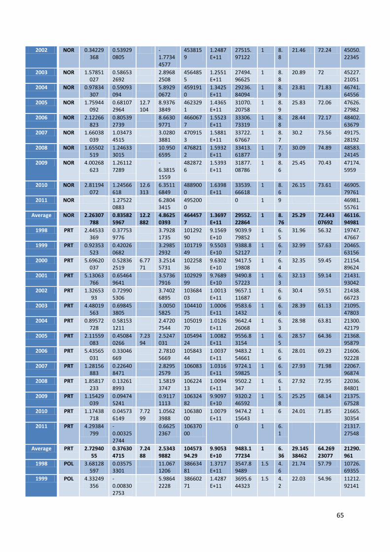
65

2002 NOR 0.34229368

0.539290805

-1.77344577

4538159

1.2487E+11

27515.97122

1 8.8

21.46 72.24 45050.22345

2003 NOR 1.57851027

0.586532692

2.89682508

4564855

1.2551E+11

27494.96625

1 8.8

20.89 72 45227.21051

2004 NOR 0.97834307

0.59093094

5.89290672

4591910

1.3425E+11

29236.84094

1 8.9

23.81 71.83 46741.64556

2005 NOR 1.75944092

0.681072964

12.7104

8.93763849

4623291

1.4365E+11

31070.20758

1 8.9

25.83 72.06 47626.27982

2006 NOR 2.12266823

0.805392739

8.66309771

4660677

1.5523E+11

33306.73319

1 8.8

28.44 72.17 48402.63679

2007 NOR 1.66038039

1.034734515

3.02803881

4709153

1.5881E+11

33722.67667

1 8.7

30.2 73.56 49175.28192

2008 NOR 1.65502519

1.246333015

10.9506595

4768212

1.5932E+11

33413.61877

1 7.9

30.09 74.89 48583.24145

2009 NOR 4.00268623

1.261127289

-6.38151559

4828726

1.5393E+11

31877.08786

1 8.6

25.45 70.43 47174.5959

2010 NOR 2.81194072

1.24566618

12.6313

6.35116849

4889000

1.6398E+11

33539.66618

1 8.6

26.15 73.61 46905.79761

2011 NOR 1.275220883

6.28043415

4952000

0 1 9 46981.55761

Average NOR 2.26307788

0.835825967

12.2882

4.86250393

4644577

1.3697E+11

29552.22864

1 8.76

25.29 72.44307692

46116.94981

1998 PRT 2.44533369

0.377539776

3.79281735

10129290

9.1569E+10

9039.979852

1 6.5

31.96 56.32 19747.47667

1999 PRT 0.92353523

0.420260682

3.29852932

10171949

9.5503E+10

9388.852127

1 6.7

32.99 57.63 20465.63156

2000 PRT 5.69620037

0.528362519

6.7771

3.25145731

10225836

9.6302E+10

9417.519808

1 6.4

32.35 59.45 21154.89624

2001 PRT 5.13063766

0.654649641

3.57367916

10292999

9.7689E+10

9490.857223

1 6.3

32.13 59.14 21431.93042

2002 PRT 1.3265393

0.729905306

3.74026895

10368403

1.0013E+11

9657.111687

1 6.6

30.4 59.51 21438.66723

2003 PRT 4.48019563

0.698453805

3.00505825

10441075

1.0006E+11

9583.61432

1 6.6

28.39 61.13 21095.47803

2004 PRT 0.89572728

0.581531211

2.47207544

10501970

1.0126E+11

9642.426068

1 6.3

28.98 63.81 21300.42179

2005 PRT 2.11559083

0.450840266

7.2394

2.5247031

10549424

1.0082E+11

9556.83154

1 6.5

28.57 64.36 21368.95879

2006 PRT 5.43565031

0.33046669

2.78105669

10584344

1.0037E+11

9483.254661

1 6.6

28.01 69.23 21606.92228

2007 PRT 1.28156883

0.226408471

2.82952579

10608335

1.0316E+11

9724.159825

1 6.5

27.93 71.98 22067.96874

2008 PRT 1.85817233

0.132618993

1.58193747

10622413

1.0094E+11

9502.2347

1 6.1

27.92 72.95 22036.84801

2009 PRT 1.15429039

0.094745241

0.91171113

10632482

9.9097E+10

9320.246592

1 5.8

25.25 68.14 21375.67528

2010 PRT 1.17438718

0.045736149

7.7299

1.05623988

10638000

1.0079E+11

9474.215643

1 6 24.01 71.85 21665.30354

2011 PRT 4.29384799

-0.003252744

0.66252367

10637000

0 1 6.1

21317.27548

Average PRT 2.7294055

0.376304715

7.2488

2.53439882

10457394.29

9.9053E+10

9483.177234

1 6.36

29.14538462

64.26923077

21290.961

1998 POL 3.68128597

0.035753301

11.0671206

38663481

1.3717E+11

3547.89489

1.5 4.6

21.74 57.79 10726.69355

1999 POL 4.33249356

-0.008302753

5.98642228

38660271

1.4287E+11

3695.644323

1.5 4.2

22.03 54.96 11212.92141

66

2000 POL 5.45493446

-0.535608109

9.5117

7.25212342

38453757

1.4735E+11

3831.758976

1.5 4.1

21.97 62.74 11753.35344

2001 POL 3.00072151

-0.536314414

3.47965753

38248076

1.4839E+11

3879.709047

1.5 4.1

18.71 60.77 11958.98287

2002 POL 2.08447471

-0.046318937

2.24590518

38230364

1.5038E+11

3933.547934

1.5 3.6

17.08 62.01 12137.23122

2003 POL 2.11668874

-0.067492702

0.39400034

38204570

1.5408E+11

4032.988783

1.5 3.6

16.97 66.71 12615.1087

2004 POL 5.03068021

-0.058512735

4.08873467

38182222

1.5994E+11

4188.830285

1 3.5

18.48 72.78 13297.13925

2005 POL 3.39209758

-0.043948953

9.6973

2.64337736

38165445

1.6914E+11

4431.694984

1 3.4

18.1 74.72 13784.16006

2006 POL 5.81731006

-0.063370574

1.48333664

38141267

1.7818E+11

4671.609386

1 3.7

19.81 81.71 14651.8488

2007 POL 5.56073462

-0.054305021

3.95598066

38120560

1.9075E+11

5003.932624

1 4.2

23.1 85.43 15654.51566

2008 POL 2.82923728

0.01363738

3.10162053

38125759

2.0313E+11

5328.023367

1 4.6

22.84 87.4 16454.80793

2009 POL 3.02219881

0.067763227

3.71793237

38151603

2.0849E+11

5464.887843

1 5 19.83 77.39 16711.31169

2010 POL 1.937921

0.084050257

9.9505

1.40346908

38184000

2.1109E+11

5528.235976

1 5.3

20.89 84.27 17348.1442

2011 POL 2.78796867

0.084599833

3.15674048

38216000

0 1 5.5

18087.44273

Average POL 3.64633908

-0.080597872

9.71983

3.85545865

38267669.64

1.6931E+11

4426.05834

1.2143

4.24

20.11923077

71.43692308

14028.11868

1998 ROM 4.82245322

-0.206980242

55.2234588

22507344

3.126E+10

1388.900519

2 3 16.95 41.27 6759.249476

1999 ROM 2.92478687

-0.156978616

47.7691848

22472040

3.1029E+10

1380.801142

2 3.3

14.8 43.6 6688.629694

2000 ROM 2.79872123

-0.12944004

9.867

44.2546316

22442971

3.1386E+10

1398.484278

2 2.9

18.09 52.69 6837.936335

2001 ROM 2.87948859

-1.395429986

37.4415236

22131970

3.3285E+10

1503.944358

2 2.8

19.78 56.99 7329.26333

2002 ROM 2.49647951

-1.496967793

23.4275355

21803129

3.5548E+10

1630.430398

2 2.8

19.49 61.99 7819.235465

2003 ROM 3.0987771

-0.28070199

23.9802842

21742013

3.7274E+10

1714.358188

2 2.8

19.7 66.13 8248.958092

2004 ROM 8.53496856

-0.263076706

15.040799

21684890

3.9798E+10

1835.282918

2.5 2.9

21.18 70.89 8965.424834

2005 ROM 6.55336941

-0.233240465

10.1337

12.2925663

21634371

4.1538E+10

1919.99338

2 3 21.05 75.71 9361.297906

2006 ROM 9.29002759

-0.21611

10.7831743

21587666

4.6775E+10

2166.749892

2 3.1

24.41 81.73 10122.69365

67

6691

2007 ROM 5.8629808

-0.189143147

13.0326971

21546873

5.3634E+10

2489.19494

2 3.7

29.71 91.95 10750.36964

2008 ROM 6.93903447

-0.154438571

11.5774121

21513622

5.82E+10

2705.26938

2 3.8

28.63 92.27 11781.85991

2009 ROM 3.00787683

-0.154537791

6.53865643

21480401

5.3988E+10

2513.36584

2 3.8

23.03 82.76 10797.07449

2010 ROM 1.81960204

-0.197584308

10.436

3.57097641

21438000

5.3269E+10

2484.778726

2 3.7

24.11 95.54 10920.97585

2011 ROM 1.52619522

-0.224157182

7.10527323

21390000

0 2 3.6

10905.38262

Average ROM 4.46819724

-0.378485252

10.1456

22.288441

21812520.71

4.2076E+10

1933.196458

2.0357

3.23

21.61 70.27076923

9092.025092

1998 SRB 0.69735174

-1.076224227

27.6877289

7567745

0 6 3 7.69 52.84 6902.974838

1999 SRB 0.63518328

-0.361977305

42.4617547

7540401

8732600000

1158.10817

5 2 8.88 30.13 6152.070499

2000 SRB 0.85301296

-0.319014864

9.2454

77.3868958

7516346

8963300000

1192.507636

4 1.3

8 27.98 6501.292217

2001 SRB 1.55817997

-0.171798903

88.3834067

7503433

9886900000

1317.650201

3 2.3

11.47 66.9 6857.642058

2002 SRB 3.75648751

-0.045339247

22.5527661

7500031

1.0344E+10

1379.194299

2.5 2.3

10.83 65.66 7143.601324

2003 SRB 7.19128522

-0.259198929

12.7427416

7480591

1.0467E+10

1399.220997

2.5 2.3

14.26 69.4 7353.719925

2004 SRB 4.34700433

-0.233056452

12.2034708

7463157

1.136E+10

1522.144047

2.5 2.7

27.86 76.48 8056.39182

2005 SRB 8.12686715

-0.29998029

9.4249

15.6818508

7440769

1.1771E+10

1581.960144

2.5 2.8

23.35 76.23 8516.986258

2006 SRB 17.0015782

-0.393204593

12.4984584

7411569

1.2634E+10

1704.632312

2.5 3 23.74 83.06 8858.360855

2007 SRB 8.81061685

-0.405458542

10.0995578

7381579

1.3726E+10

1859.493748

2.5 3.4

28.56 87.36 9374.645689

2008 SRB 6.27376212

-0.425719157

12.6080152

7350221

1.4495E+10

1972.049548

2.5 3.4

29.32 89.89 9772.39676

2009 SRB 4.82120212

-0.4009813

5.64462192

7320807

0 2 3.5

17.53 76.71 9468.25278

2010 SRB 3.48617589

-0.402005901

9.5538

9.09589532

7291000

0 2 3.5

17.35 88.13 9597.083308

2011 SRB 5.99530619

-0.418294839

8.60499504

7261000

1.7622E+10

2426.938438

2 3.3

9809.000194

68

Average SRB 5.25385811

-0.372303896

9.40803

25.5465828

7430617.786

1.1818E+10

1592.172685

2.9643

2.77

17.60307692

68.52076923

8168.887037

1998 SVK 1.91996099

0.134121598

5.07325709

5390516

2.2071E+10

4094.404996

2 3.9

26.49 110.27 12545.74014

1999 SVK 1.18307559

0.102053161

7.36160934

5396020

2.1785E+10

4037.151668

1.5 3.7

22.25 117.05 12537.67365

2000 SVK 7.14551547

-0.135376488

11.2079

9.41714814

5388720

2.2489E+10

4173.298544

1.5 3.5

21.18 125.2 12726.45514

2001 SVK -0.183012271

5.01671439

5378867

2.3201E+10

4313.354872

1.5 3.7

23.8 133.33 13193.71305

2002 SVK 11.8487277

0.003513689

3.87409235

5379056

2.4219E+10

4502.41769

1.5 3.7

23.03 133.4 13797.88191

2003 SVK 1.22010672

0.010242908

5.31000063

5379607

2.4002E+10

4461.625633

1.5 3.7

20.05 142.15 14455.25378

2004 SVK 5.41687959

0.05261082

5.84856941

5382438

2.5758E+10

4785.561745

1 4 22.23 146.81 15178.38465

2005 SVK 3.93150531

0.084739795

11.6028

2.38184062

5387001

2.8014E+10

5200.370385

1 4.3

24.34 153.55 16174.8268

2006 SVK 6.03889945

0.081793145

2.94194631

5391409

3.0335E+10

5626.555526

1 4.7

23.85 169.23 17510.3539

2007 SVK 3.99882142

0.109540275

1.11284652

5397318

3.3663E+10

6236.991146

1 4.9

23.68 171.09 19326.69704

2008 SVK 3.29982463

0.172307489

2.86078438

5406626

3.5651E+10

6593.92738

1 5 23.41 166.61 20402.88841

2009 SVK -0.03616

87

0.221039559

-1.18157029

5418590

3.3252E+10

6136.687224

1 4.5

17.07 144.47 19353.87576

2010 SVK 0.635231

0.212173182

11.5629

0.4916413

5430000

3.7114E+10

6835.036068

1 4.3

19.99 161.42 20120.69302

2011 SVK 0.182169504

1.63783974

5440000

0 1 4 20756.72951

Average SVK 3.8835316

0.074851169

11.4579

3.72476571

5397583.429

2.7812E+10

5153.644837

1.25

4.14

22.41307692

144.1984615

16291.51191

1998 SVN 0.99184428

-0.218117657

7.03190335

1981629

1.5318E+10

7729.902044

1.5 5.9

28.06 100.38 18065.32831

1999 SVN 0.4778194

0.071430845

6.56828601

1983045

1.6276E+10

8207.639206

1.5 6 30.83 99.48 19013.83164

2000 SVN 0.67969778

0.29607496

11.5642

5.22337966

1988925

1.6538E+10

8314.858045

1.5 5.5

30.35 105.02 19766.26283

2001 SVN 2.4557383

0.157498742

8.65155603

1992060

1.7271E+10

8669.705826

1.5 5.2

28.7 107.1 20315.29699

2002 SVN 7.17269504

0.123915442

7.58475371

1994530

1.8103E+10

9076.446469

1 5.9

28.47 109.17 21066.6121

2003 SVN 1.0342318

0.060296779

5.53278974

1995733

1.8855E+10

9447.734702

1 5.9

30.39 110.89 21670.80352

2004 SVN 2.45701917

0.064066202

3.27081632

1997012

1.9522E+10

9775.801833

1 6 32.04 119.74 22610.2203

2005 SVN 1.51297393

0.173208905

11.5984

1.66005894

2000474

2.0139E+10

10067.12159

1 6.1

30.89 125.2 23475.57268

2006 SVN 1.66729982

0.319114537

2.1136444

2006868

2.1271E+10

10598.8924

1 6.4

32.73 132.5 24769.63065

2007 SVN 3.2371133

0.559207816

4.17296943

2018122

2.2707E+10

11251.32135

1 6.6

36.26 141.85 26323.73439

2008 SVN 3.54686761

0.158140844

4.12435758

2021316

2.3039E+10

11397.93478

1 6.7

36.35 141.6 27225.48029

2009 SVN -1.30618

0.903875535

2.96371089

2039669

2.1606E+10

10592.75469

1 6.6

26.71 127.79 24819.94394

69

33

2010 SVN 0.78059052

0.436079485

11.7049

-1.06698039

2049000

2.2302E+10

10884.487

1 6.4

26.32 136.64 25052.85592

2011 SVN 2.21230888

0.166659267

0.80499593

2052000

0 1 5.9

24967.46976

Average SVN 1.92285832

0.233675122

11.6225

4.18830297

2008598.786

1.9457E+10

9693.430764

1.1429

6.08

30.62307692

119.7969231

22795.93167

1998 ESP 2.3770548

0.34978306

2.48006884

39721108

4.5895E+11

11554.38738

1.5 6.1

26.5 47.41 23165.56868

1999 ESP 2.99789616

0.515171909

2.62698262

39926268

4.7939E+11

12006.96502

1.5 6.6

27.99 49.86 24140.30709

2000 ESP 6.69173192

0.840384465

9.0939

3.39429573

40263216

4.9645E+11

12330.05573

1.5 7 28.25 52.43 25147.12499

2001 ESP 4.62566002

1.129296043

4.19220821

40720484

5.1272E+11

12591.20716

1.5 7 28.44 52.74 25777.13127

2002 ESP 5.82740165

1.446951382

4.35308949

41313973

5.2976E+11

12822.70152

1 6.9

28.64 52.85 26095.40574

2003 ESP 2.89723163

1.657650711

4.16260967

42004522

5.4859E+11

13060.36127

1 6.9

29.24 53.81 26459.34904

2004 ESP 2.3732789

1.622698513

4.04264134

42691689

5.6155E+11

13153.51168

1 7.1

29.8 55.82 26881.96717

2005 ESP 2.17303122

1.641238788

9.703

4.34394447

43398143

5.7947E+11

13352.43449

1 7 30.7 56.87 27392.04339

2006 ESP 2.52126819

1.641587259

4.14048309

44116441

5.9933E+11

13585.2055

1 6.8

32.01 59.48 28044.43046

2007 ESP 4.62610741

1.713622904

3.26768225

44878945

6.1586E+11

13722.66333

1 6.7

32.28 61.81 28527.08873

2008 ESP 4.88890341

1.49673505

2.37444942

45555716

6.1061E+11

13403.65194

1 6.5

30.68 59.28 28353.03543

2009 ESP 0.66661385

0.771622835

0.07373032

45908594

5.926E+11

12908.24282

1 6.1

26.99 52.65 27082.63438

2010 ESP 2.9754832

0.353072269

10.3503

0.40483123

46071000

6.1782E+11

13410.14937

1 6.1

25.28 57.15 26968.43187

2011 ESP 1.71979159

0.355403168

1.37875017

46235000

0 1 6.2

27063.00162

Average ESP 3.382961

1.109658454

9.71573

2.94541192

43057507.07

5.5408E+11

12915.50286

1.1429

6.64

28.98461538

54.78153846

26506.96571

1998 SWE 7.85843472

0.055512122

0.53392908

8850974

1.9926E+11

22513.30673

1 9.5

17.62 77.68 26724.50151

1999 SWE 23.4248638

0.077927151

0.89809775

8857874

2.0642E+11

23303.14984

1 9.4

17.82 78.91 27948.03235

2000 SWE 9.658416

0.160575485

10.9885

1.42456061

8872109

2.1382E+11

24100.78805

1 9.4

18.5 84.6 29145.49446

2001 SWE 4.94521271

0.268470528

2.37026957

8895960

2.1439E+11

24100.17806

1 9 18 83.11 29434.27256

2002 SWE 4.93641082

0.325438068

1.53277716

8924958

2.1846E+11

24477.96518

1 9.3

17.13 81.15 30067.23867

2003 SWE 1.5915008

0.372092943

1.76594496

8958229

2.2835E+11

25490.42061

1 9.3

17.24 82.48 30655.24124

2004 SWE 3.3467929

0.393298991

0.31358972

8993531

2.3413E+11

26033.62942

1 9.2

17.2 86.18 31828.02254

2005 SWE 3.27275002

0.399942763

11.7296

0.88562123

9029572

2.4186E+11

26785.3379

1 9.2

18.01 89.2 32702.98278

2006 SWE 7.13838552

0.562483906

1.94226521

9080505

2.5368E+11

27936.58806

1 9.2

19.07 93.18 33916.97341

2007 SWE 6.00812089

0.741552515

2.75965981

9148092

2.6663E+11

29146.174

1 9.3

20.77 96.64 34782.1783

2008 SWE 7.85539007

0.779033291

3.13751015

9219637

2.6601E+11

28852.5392

1 9.3

20.66 99.74 34300.56246

70

2009 SWE 2.41187016

0.851904413

2.05621443

9298515

2.4454E+11

26298.44737

1 9.2

16.66 91.04 32299.67999

2010 SWE -0.40340

26

0.852524629

11.615

1.02222708

9378000

2.5963E+11

27684.73253

1 9.2

18.82 96.4 33995.91437

2011 SWE 2.28241388

0.795219517

0.90859582

9453000

0 1 9.3

35047.55917

Average SWE 6.02336855

0.473998309

11.4444

1.5393759

9068639.714

2.344E+11

25901.789

1 9.27

18.26923077

87.71615385

31632.0467

1998 CHE 3.53923568

0.297135766

0.2891813

7110001

2.1361E+11

30042.93223

1 8.9

28.92 74.17 33424.50479

1999 CHE 4.63291222

0.476919931

0.61493598

7143991

2.1705E+11

30381.55761

1 8.9

27.11 77.48 33701.63124

2000 CHE 7.90834017

0.561954617

9.9885

1.13163993

7184250

2.2426E+11

31215.17489

1 8.6

26.63 83.44 34713.23698

2001 CHE 3.68344143

0.632771238

0.79532497

7229854

2.1806E+11

30160.36634

1 8.4

26.34 83.64 34891.67646

2002 CHE 2.43537049

0.756469146

0.46983292

7284753

2.1834E+11

29971.56453

1 8.8

26.08 82.83 34782.18162

2003 CHE 5.37499249

0.741919603

0.99945594

7339001

2.3077E+11

31444.58246

1 8.8

25.83 83.39 34456.792

2004 CHE 0.51132781

0.68742596

0.57069173

7389625

2.3574E+11

31902.13011

1 9.1

26.07 87.5 35087.44703

2005 CHE -0.14096

19

0.64060154

10.0288

0.10818392

7437115

2.4584E+11

33055.72136

1 9.1

26 91.41 35784.01319

2006 CHE 11.50022

0.627558473

2.06130403

7483934

2.4949E+11

33336.144

1 9.1

25.48 95.76 36851.12207

2007 CHE 7.69616165

0.893690978

2.49360982

7551117

2.4047E+11

31845.57214

1 9 24.51 99.86 37854.35512

2008 CHE 3.18029897

1.270618074

2.44493291

7647675

2.2206E+11

29036.32521

1 9 23.38 99.76 38159.62633

2009 CHE 5.95182475

1.249484631

0.16040647

7743831

2.6117E+11

33726.3771

1 9 23.11 94.49 36978.0434

2010 CHE 4.10026222

1.057454743

10.2632

0.06965132

7826000

2.784E+11

35574.12096

1 8.7

22.85 99.36 37582.12145

2011 CHE 0.42141151

1.027736927

0.6396954

7907000

0 1 8.8

37979.00906

Average CHE 4.34248839

0.780124402

10.0935

0.91777476

7448439.071

2.3502E+11

31668.65915

1 8.87

25.56230769

88.69923077

35874.6972

1998 TUR 0.34906982

1.566161411

137.964853

61742674

2.4681E+11

3997.431259

4.5 3.4

19.06 37.95 9815.450293

1999 TUR 0.31351167

1.526834476

54.1790075

62692616

2.3781E+11

3793.348843

4.5 3.6

17.5 36.06 9341.404356

2000 TUR 0.36838695

1.480778262

5.5449

49.2258732

63627862

2.4906E+11

3914.345878

4.5 3.8

19.13 40.32 9827.625473

2001 TUR 1.71015793

1.430986638

52.850551

64544914

2.2949E+11

3555.45197

4.5 3.6

13.34 37.95 9136.023638

2002 TUR 0.46530718

1.386657374

37.4248384

65446165

2.4329E+11

3717.405926

3.5 3.1

16.2 40.47 9565.587659

2003 TUR 0.56170634

1.355659031

23.2703148

66339433

2.6043E+11

3925.775672

3.5 3.1

16.95 43.82 9933.657685

2004 TUR 0.71015796

1.342324604

12.3998734

67235927

2.6995E+11

4014.902025

3 3.2

18.17 46.44 10718.87495

2005 TUR 2.07689829

1.340343517

6.0568

7.08429226

68143186

2.9448E+11

4321.534672

3 3.5

19.83 47.17 11464.73258

2006 TUR 3.8020336

1.341575365

9.33086822

69063538

3.1E+11

4488.668769

3 3.8

21.05 47.18 12091.73982

2007 TUR 3.40675658

1.336480094

6.22093193

69992754

3.2635E+11

4662.684982

3 4.1

21.24 49.08 12488.22926

71

2008 TUR 2.67054617

1.321335189

11.9944161

70923730

3.2351E+11

4561.335324

3 4.6

20.11 48.31 12405.50061

2009 TUR 1.36863499

1.292281589

5.29434107

71846212

3.103E+11

4318.896136

3 4.4

14.96 45.37 11655.2308

2010 TUR 1.23614434

1.253297411

6.4748

5.67573972

72752000

3.3722E+11

4635.201748

3 4.4

20.29 46.83 12564.03914

2011 TUR 2.05357359

1.21220059

8.62527039

73639596

0 3 4.2

13466.33282

Average TUR 1.50663467

1.370493968

6.0255

30.1100836

67713614.79

2.799E+11

4146.691016

3.5 3.77

18.29461538

43.61153846

11033.88779

1998 UKR 1.77397922

-0.893741564

12.0120189

50143939

2.2746E+10

453.6132822

3.5 2.8

13.32 96.34 3429.970333

1999 UKR 1.57058253

-0.942908046

27.3999247

49673349

2.2347E+10

449.8729416

3.5 2.6

10.89 86.11 3455.539826

2000 UKR 1.90329792

-1.006597042

10.6584

23.1159426

49175847

2.285E+10

464.6540211

4 1.5

12.86 100.09 3696.438272

2001 UKR 2.08369812

-1.005494904

9.94718615

48683864

2.4799E+10

509.387231

4 2.1

13.96 96.44 4077.302237

2002 UKR 1.63470785

-0.993676542

5.1218419

48202500

2.7106E+10

562.3373796

4 2.3

12.9 95.46 4332.156404

2003 UKR 2.84044706

-0.811436362

8.22060286

47812950

2.8767E+10

601.6649981

4 2.3

14.64 98.55 4777.992602

2004 UKR 2.64321686

-0.758627911

15.1556536

47451600

3.2902E+10

693.3748912

3.5 2.2

13.63 103.18 5396.917319

2005 UKR 9.06410156

-0.732790732

11.1192

24.5522927

47105150

3.5149E+10

746.1868105

2.5 2.6

14.81 94.51 5583.399175

2006 UKR 5.20077993

-0.676092035

14.8782516

46787750

3.9119E+10

836.1041487

2.5 2.8

16.19 87.69 6031.629136

2007 UKR 6.93040122

-0.596804887

22.7526076

46509350

4.5056E+10

968.7474874

2.5 2.7

18.68 90.76 6547.084842

2008 UKR 6.06303358

-0.541462211

28.583474

46258200

4.8032E+10

1038.339997

2.5 2.5

18.18 97.3 6734.031492

2009 UKR 4.1082416

-0.443932417

13.0736131

46053300

3.6964E+10

802.6342746

2.5 2.2

8.64 73.81 5762.921606

2010 UKR 4.76108017

-0.397285236

11.2817

13.8596912

45871000

4.0207E+10

876.5252952

3 2.4

9.45 76.19 6023.08274

2011 UKR 4.3614025

-0.359480081

15.6065722

45706100

0 3.5 2.3

6359.101708

Average UKR 3.92421215

-0.725737855

11.0198

16.7342624

47531064.21

3.2773E+10

692.5725199

3.25

2.38

13.70384615

92.03307692

5157.683407

1998 GBR 5.12705989

0.291406085

2.00431964

58487141

1.2168E+12

20804.15161

1.5 8.7

18.71 48.87 27021.47898

1999 GBR 5.94476586

0.333405882

1.92912191

58682466

1.2391E+12

21115.0655

1.5 8.6

18.54 49.53 27916.07171

2000 GBR 8.26948133

0.357300887

8.5824

0.61891257

58892514

1.2783E+12

21706.48139

1.5 8.7

18.14 51.92 29056.46827

72

2001 GBR 3.66123966

0.365161651

1.44816455

59107960

1.3366E+12

22613.17193

1.5 8.3

18.24 52.36 29862.69405

2002 GBR 1.58409118

0.367883666

2.53564952

59325809

1.3995E+12

23589.42102

1 8.7

17.88 52.86 30543.72469

2003 GBR 1.48427803

0.404485063

2.35076281

59566259

1.453E+12

24392.96005

1 8.7

17.93 52.04 31492.63429

2004 GBR 2.60440046

0.505061081

2.49376652

59867866

1.4951E+12

24973.57132

1 8.6

18.3 53.56 32260.00078

2005 GBR 7.77908736

0.593614118

8.9762

2.18692471

60224307

1.5169E+12

25187.1026

1 8.6

18.29 56.45 32737.9538

2006 GBR 6.30457993

0.614676968

3.23266328

60595632

1.5421E+12

25448.8439

1 8.6

18.93 60.96 33385.62467

2007 GBR 7.18380223

0.64321601

2.26586372

60986649

1.6151E+12

26482.63868

1 8.4

20.07 58.18 34321.35301

2008 GBR 3.54731642

0.664933705

3.13445115

61393521

1.6007E+12

26072.75252

1 7.7

18.99 58.88 33717.8864

2009 GBR 3.35838735

0.677747055

1.65494344

61811027

1.5161E+12

24528.40366

1 7.7

16.14 55.14 32025.50077

2010 GBR 2.35215485

0.677688813

9.4176

2.86140664

62232000

1.4868E+12

23891.84334

1 6.7

17.43 57.29 32474.70243

2011 GBR 2.23137081

0.65613487

2.3258903

62641000

0 1 7.8

32473.54772

Average GBR 4.3880011

0.510908275

8.99207

2.21734577

60272439.36

1.4382E+12

23908.18519

1.1429

8.27

18.27615385

54.46461538

31377.83154

1998 RUS 0.46862425

-0.275320276

18.538687

146899000

2.0015E+11

1362.500766

4 2.4

9.66 42.11 7328.874682

1999 RUS 1.12687851

-0.402445224

72.3867777

146309000

2.0944E+11

1431.490886

4.5 2.4

8.69 41.5 7829.368262

2000 RUS 1.22320796

-0.004100994

4.7718

37.6980956

146303000

2.5971E+11

1775.151569

5 2.1

13.83 43.49 8612.658286

2001 RUS 0.82601315

-0.241859173

16.489528

145949580.3

2.6656E+11

1826.384148

5 2.3

15.25 44.54 9073.131172

2002 RUS 1.02362861

-0.44627828

15.4929534

145299690.3

2.7675E+11

1904.684032

5 2.7

14.08 47.16 9546.037536

2003 RUS 2.26029466

-0.483095546

13.7800615

144599446.7

3.0648E+11

2119.510184

5 2.7

14.95 50.01 10292.10332

2004 RUS 2.33191834

-0.519935361

20.2820769

143849574.2

3.5476E+11

2466.187348

5.5 2.8

15.48 53.37 11088.16108

2005 RUS 1.67113349

-0.487509848

4.8285

19.3060948

143150000

4.0884E+11

2856.025148

5.5 2.4

15.84 54.91 11852.80594

2006 RUS 2.33864915

-0.455103184

15.1700471

142500000

4.6784E+11

3283.087719

5.5 2.5

17.3 57.38 12877.69003

2007 RUS 3.5327704

-0.281096461

13.8044207

142100000

5.1708E+11

3638.845883

5.5 2.3

19.51 60.72 14016.15479

2008 RUS 3.34730209

-0.105615218

17.959714

141950000

6.1858E+11

4357.731596

5.5 2.1

20.58 61.98 14767.30437

2009 RUS 3.57134885

-0.028182907

2.0061638

141910000

0 5.5 2.2

13.48 53.72 13614.5467

73

2010 RUS 3.5308956

0.007046471

4.8215

11.6039809

141920000

0 5.5 2.1

17.72 49.27 14198.97165

2011 RUS 3.62172853

0.007045975

15.8557119

141930000

6.6373E+11

4676.460227

5.5 2.4

14808.48399

Average RUS 2.20531383

-0.265460716

4.80727

20.7410224

143904949.4

3.7916E+11

2438.31227

5.1786

2.39

15.10538462

50.78153846

11421.87798

RASMUS UNIV RSITY ROTT R AM Thesis Marin... · Emami Namini and his feedback and advice on my work....

Documents

Transcript of RASMUS UNIV RSITY ROTT R AM Thesis Marin... · Emami Namini and his feedback and advice on my work....