Radial Basis Function
35
International Scholarly Research Network ISRN Applied Mathematics Volume 2012, Article ID 324194, 34 pages doi:10.5402/2012/324194 Review Article Using Radial Basis Function Networks for Function Approximation and Classification Yue Wu, 1 Hui Wang, 1 Biaobiao Zhang, 1 and K.-L. Du 1, 2 1 Enjoyor Laboratories, Enjoyor Inc., Hangzhou 310030, China 2 Department of Electrical and Computer Engineering, Concordia University, Montreal, QC, Canada H3G 1M8 Correspondence should be addressed to K.-L. Du, [email protected] Received 16 November 2011; Accepted 5 December 2011 Academic Editors: E. Gallopoulos, E. Kita, and M. Sun Copyright q 2012 Yue Wu et al. This is an open access article distributed under the Creative Commons Attribution License, which permits unrestricted use, distribution, and reproduction in any medium, provided the original work is properly cited. The radial basis function RBF network has its foundation in the conventional approximation the- ory. It has the capability of universal approximation. The RBF network is a popular alternative to the well-known multilayer perceptron MLP, since it has a simpler structure and a much faster training process. In this paper, we give a comprehensive survey on the RBF network and its learn- ing. Many aspects associated with the RBF network, such as network structure, universal approxi- mation capability, radial basis functions, RBF network learning, structure optimization, normal- ized RBF networks, application to dynamic system modeling, and nonlinear complex-valued sig- nal processing, are described. We also compare the features and capability of the two models. 1. Introduction The multilayer perceptron MLP trained with backpropagation BP rule 1 is one of the most important neural network models. Due to its universal function approximation capabil- ity, the MLP is widely used in system identification, prediction, regression, classification, con- trol, feature extraction, and associative memory 2. The RBF network model was proposed by Broomhead and Lowe in 1988 3. It has its foundation in the conventional approximation techniques, such as generalized splines and regularization techniques. The RBF network has equivalent capabilities as the MLP model, but with a much faster training speed, and thus it has become a good alternative to the MLP. The RBF network has its origin in performing exact interpolation of a set of data points in a multidimensional space 4. It can be considered one type of functional link nets 5. It has a network architecture similar to the classical regularization network 6, where the basis functions are the Green’s functions of the Gram’s operator associated with the stabilizer. If the stabilizer exhibits radial symmetry, an RBF network is obtained. From the viewpoint of
-
Upload
nicolas-br -
Category
Documents
-
view
30 -
download
6
description
Artigo que discute a estrutura das funcoes de base radial
Transcript of Radial Basis Function

International Scholarly Research NetworkISRN Applied MathematicsVolume 2012, Article ID 324194, 34 pagesdoi:10.5402/2012/324194
Review ArticleUsing Radial Basis Function Networks forFunction Approximation and Classification
Yue Wu,1 Hui Wang,1 Biaobiao Zhang,1 and K.-L. Du1, 2
1 Enjoyor Laboratories, Enjoyor Inc., Hangzhou 310030, China2 Department of Electrical and Computer Engineering, Concordia University, Montreal,QC, Canada H3G 1M8
Correspondence should be addressed to K.-L. Du, [email protected]
Received 16 November 2011; Accepted 5 December 2011
Academic Editors: E. Gallopoulos, E. Kita, and M. Sun
Copyright q 2012 Yue Wu et al. This is an open access article distributed under the CreativeCommons Attribution License, which permits unrestricted use, distribution, and reproduction inany medium, provided the original work is properly cited.
The radial basis function (RBF) network has its foundation in the conventional approximation the-ory. It has the capability of universal approximation. The RBF network is a popular alternative tothe well-known multilayer perceptron (MLP), since it has a simpler structure and a much fastertraining process. In this paper, we give a comprehensive survey on the RBF network and its learn-ing. Many aspects associated with the RBF network, such as network structure, universal approxi-mation capability, radial basis functions, RBF network learning, structure optimization, normal-ized RBF networks, application to dynamic system modeling, and nonlinear complex-valued sig-nal processing, are described. We also compare the features and capability of the two models.
1. Introduction
The multilayer perceptron (MLP) trained with backpropagation (BP) rule [1] is one of themost important neural network models. Due to its universal function approximation capabil-ity, the MLP is widely used in system identification, prediction, regression, classification, con-trol, feature extraction, and associative memory [2]. The RBF network model was proposedby Broomhead and Lowe in 1988 [3]. It has its foundation in the conventional approximationtechniques, such as generalized splines and regularization techniques. The RBF network hasequivalent capabilities as the MLP model, but with a much faster training speed, and thus ithas become a good alternative to the MLP.
The RBF network has its origin in performing exact interpolation of a set of data pointsin a multidimensional space [4]. It can be considered one type of functional link nets [5]. Ithas a network architecture similar to the classical regularization network [6], where the basisfunctions are the Green’s functions of the Gram’s operator associated with the stabilizer. Ifthe stabilizer exhibits radial symmetry, an RBF network is obtained. From the viewpoint of
2 ISRN Applied Mathematics
x2
x1
xJ1
y2
y1
yJ3
.........
φ2
φ1
φJ2
φ0 = 1
∑∑
∑
w
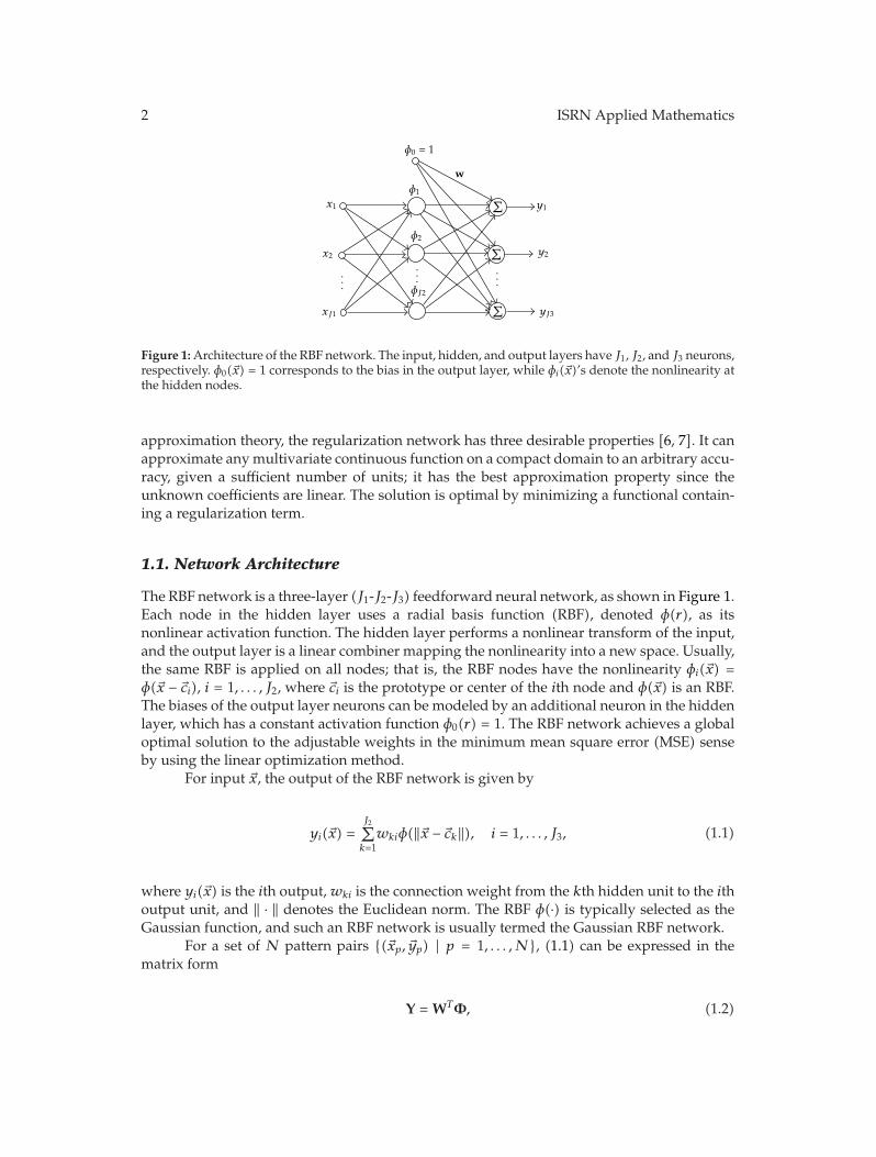
Figure 1: Architecture of the RBF network. The input, hidden, and output layers have J1, J2, and J3 neurons,respectively. φ0(�x) = 1 corresponds to the bias in the output layer, while φi(�x)’s denote the nonlinearity atthe hidden nodes.
approximation theory, the regularization network has three desirable properties [6, 7]. It canapproximate any multivariate continuous function on a compact domain to an arbitrary accu-racy, given a sufficient number of units; it has the best approximation property since theunknown coefficients are linear. The solution is optimal by minimizing a functional contain-ing a regularization term.
1.1. Network Architecture
The RBF network is a three-layer (J1-J2-J3) feedforward neural network, as shown in Figure 1.Each node in the hidden layer uses a radial basis function (RBF), denoted φ(r), as itsnonlinear activation function. The hidden layer performs a nonlinear transform of the input,and the output layer is a linear combiner mapping the nonlinearity into a new space. Usually,the same RBF is applied on all nodes; that is, the RBF nodes have the nonlinearity φi(�x) =φ(�x − �ci), i = 1, . . . , J2, where �ci is the prototype or center of the ith node and φ(�x) is an RBF.The biases of the output layer neurons can be modeled by an additional neuron in the hiddenlayer, which has a constant activation function φ0(r) = 1. The RBF network achieves a globaloptimal solution to the adjustable weights in the minimum mean square error (MSE) senseby using the linear optimization method.
For input �x, the output of the RBF network is given by
yi(�x) =J2∑k=1wkiφ(‖�x − �ck‖), i = 1, . . . , J3, (1.1)
where yi(�x) is the ith output, wki is the connection weight from the kth hidden unit to the ithoutput unit, and ‖ · ‖ denotes the Euclidean norm. The RBF φ(·) is typically selected as theGaussian function, and such an RBF network is usually termed the Gaussian RBF network.
For a set of N pattern pairs {(�xp, �yp) | p = 1, . . . ,N}, (1.1) can be expressed in thematrix form
Y = WTΦ, (1.2)

ISRN Applied Mathematics 3
where W = [ �w1, . . . , �wJ3] is a J2 × J3 matrix, �wi = (w1i, . . . , wJ2i)T , Φ = [�φ1, . . . , �φN] is a J2 ×N
matrix, �φp = (φp,1, . . . ,φp,J2)T is the output of the hidden layer for the pth sample, that is,
φp,k = φ(‖�xp − �ck‖), Y = [�y1 �y2 . . . �yN] is a J3 ×N matrix, and �yp = (yp,1, . . . ,yp,J3)T .
The RBF network with a localized RBF such as the Gaussian RBF network is a recep-tive-field or localized network. The localized approximation method provides the strongestoutput when the input is near the prototype of a node. For a suitably trained localized RBFnetwork, input vectors that are close to each other always generate similar outputs, whiledistant input vectors produce nearly independent outputs. This is the intrinsic local gener-alization property. A receptive-field network is an associative neural network in that only asmall subspace is determined by the input to the network. This property is particularly attrac-tive since the modification of the receptive-field function produces local effect. Thus recep-tive-field networks can be conveniently constructed by adjusting the parameters of the recep-tive-field functions and/or adding or removing neurons. Another well-known receptive-fieldnetwork is the cerebellar model articulation controller (CMAC) [8, 9]. The CMAC is a dis-tributed LUT system suitable for VLSI realization. It can approximate slow-varying functions,but may fail in approximating highly nonlinear or rapidly oscillating functions [10, 11].
1.2. Universal Approximation
The RBF network has universal approximation and regularization capabilities. Theoretically,the RBF network can approximate any continuous function arbitrarily well, if the RBF issuitably chosen [6, 12, 13]. A condition for suitable φ(·) is given by Micchelli’s interpolationtheorem [14]. A less restrictive condition is given in [15], where φ(·) is continuous on (0,∞)and its derivatives satisfy (−1)lφ(l)(x) > 0, for all x ∈ (0,∞) and l = 0, 1, 2. The choice of RBFis not crucial to the performance of the RBF network [4, 16]. The Gaussian RBF network canapproximate, to any degree of accuracy, any continuous function by a sufficient number ofcenters �ci, i = 1, . . . , J2, and a common standard deviation σ > 0 in the Lp norm, p ∈ [1,∞][12]. A class of RBF networks can achieve universal approximation when the RBF is con-tinuous and integrable [12]. The requirement of the integrability of the RBF is relaxed in [13].For an RBF which is continuous almost everywhere, locally essentially bounded and non-polynomial, the RBF network can approximate any continuous function with respect to theuniform norm [13]. Based on this result, such RBFs as φ(r) = e−r/σ
2and φ(r) = er/σ
2also lead
to universal approximation capability [13].In [17], in an incremental constructive method three-layer feedforward networks with
randomly generated hidden nodes are proved to be universal approximators when anybounded nonlinear piecewise continuous activation function is used, and only the weightslinking the hidden layer and the output layer need to be adjusted. The proof itself givesan efficient incremental construction of the network. Theoretically the learning algorithmsthus derived can be applied to a wide variety of activation functions no matter whether theyare sigmoidal or nonsigmoidal, continuous or noncontinuous, or differentiable or nondiffe-rentiable; it can be used to train threshold networks directly. The network learning process isfully automatic, and no user intervention is needed.
This paper is organized as follows. In Section 2, we give a general description to avariety of RBFs. Learning of the RBF network is treated in Section 3. Optimization of the RBFnetwork structure and model selection is described in Section 4. In Section 5, we introduce thenormalized RBF network. Section 6 describes the applications of the RBF network to dynamicsystems and complex RBF networks to complex-valued signal processing. A comparison

4 ISRN Applied Mathematics
between the RBF network and the MLP is made in Section 7. A brief summary is given inSection 8, where topics such as generalizations of the RBF network, robust learning againstoutliers, and hardware implementation of the RBF network are also mentioned.
2. Radial Basis Functions
A number of functions can be used as the RBF [6, 13, 14]
φ(r) = e−r2/2σ2
, Gaussian, (2.1)
φ(r) =1
(σ2 + r2)α, α > 0, (2.2)
φ(r) =(σ2 + r2
)β, 0 < β < 1, (2.3)
φ(r) = r, linear, (2.4)
φ(r) = r2 ln(r), thin-plate spline, (2.5)
φ(r) =1
1 + e(r/σ2)−θ , logistic function, (2.6)
where r > 0 denotes the distance from a data point �x to a center �c, σ in (2.1), (2.2), (2.3), and(2.6) is used to control the smoothness of the interpolating function, and θ in (2.6) is an adjus-table bias. When β in (2.3) takes the value of 1/2, the RBF becomes Hardy’s multiquadricfunction, which is extensively used in surface interpolation with very good results [6]. Whenα in (2.2) is unity, φ(r) is suitable for DSP implementation [18].
Among these RBFs, (2.1), (2.2), and (2.6) are localized RBFs with the property thatφ(r) → 0 as r → ∞. Physiologically, there exist Gaussian-like receptive fields in cortical cells[6]. As a result, the RBF is typically selected as the Gaussian. The Gaussian is compact andpositive. It is motivated from the point of view of kernel regression and kernel density esti-mation. In fitting data in which there is normally distributed noise with the inputs, theGaussian is the optimal basis function in the least-squares (LS) sense [19]. The Gaussian isthe only factorizable RBF, and this property is desirable for hardware implementation of theRBF network.
Another popular RBF for universal approximation is the thin-plate spline function(2.5), which is selected from a curve-fitting perspective [20]. The thin-plate spline is the solu-tion when fitting a surface through a set of points and by using a roughness penalty [21]. Itdiverges at infinity and is negative over the region of r ∈ (0, 1). However, for training pur-pose, the approximated function needs to be defined only over a specified range. There issome limited empirical evidence to suggest that the thin-plate spline better fits the data inhigh-dimensional settings [20]. The Gaussian and the thin-plate spline functions are illus-trated in Figure 2.
A pseudo-Gaussian function in the one-dimensional space is introduced by selectingthe standard deviation σ in the Gaussian (2.1) as two different positive values, namely, σ− forx < 0 and σ+ for x > 0 [22]. This function is extended to the multiple dimensional space bymultiplying the pseudo-Gaussian function in each dimension. The pseudo-Gaussian function

ISRN Applied Mathematics 5
−1−2 0 1 2−0.5
0
0.5
1
1.5
2
2.5
xGaussianThin plate
φ(r)
Figure 2: The Gaussian and thin-plate spline functions. r = |x|.
is not strictly an RBF due to its radial asymmetry, and this, however, provides the hiddenunits with a greater flexibility with respect to function approximation.
Approximating functions with nearly constant-valued segments using localized RBFsis most difficult, and the approximation is inefficient. The sigmoidal RBF, as a composite of aset of sigmoidal functions, can be used to deal with this problem [23]
φ(x) =1
1 + e−β[(x−c)+θ]− 1
1 + e−β[(x−c)−θ], (2.7)
where θ > 0 and β > 0. φ(x) is radially symmetric with the maximum at c. β controls the steep-ness, and θ controls the width of the function. The shape of φ(x) is approximately rectangularor more exactly soft trapezoidal if β × θ is large. For small β and θ it is bell shaped. φ(x) canbe extended for n-dimensional approximation by multiplying the corresponding function ineach dimension. To accommodate constant values of the desired output and to avoid dimini-shing the kernel functions, φ(�x) can be modified by adding a compensating term to the pro-duct term φi(xi) [24]. An alternative approach is to use the raised-cosine function as a one-dimensional RBF [25]. The raised-cosine RBF can represent a constant function exactly usingtwo terms. This RBF can be generalized to n dimensions [25]. Some popular fuzzy member-ship functions can serve the same purpose by suitably constraining some parameters [2].
The popular Gaussian RBF is circular shaped. Many RBF nodes may be required forapproximating a functional behavior with sharp noncircular features. In order to reduce thesize of the RBF network, direction-dependent scaling, shaping, and rotation of Gaussian RBFsare introduced in [26] for maximal trend sensing with minimal parameter representations forfunction approximation, by using a directed graph-based algorithm.
3. RBF Network Learning
RBF network learning can be formulated as the minimization of the MSE function
E =1N
N∑i=1
∥∥∥�yp −WT �φp∥∥∥2
=1N
∥∥∥Y −WTΦ∥∥∥2
F, (3.1)

6 ISRN Applied Mathematics
where Y = [�y1, �y2, . . . , �yN], �yi is the target output for the ith sample in the training set, and‖ · ‖2
F is the Frobenius norm defined as ‖A‖2F = tr(ATA).
RBF network learning requires the determination of the RBF centers and the weights.Selection of the RBF centers is most critical to RBF network implementation. The centers canbe placed on a random subset or all of the training examples, or determined by clustering orvia a learning procedure. One can also use all the data points as centers in the beginning andthen selectively remove centers using the k-NN classification scheme [27]. For some RBFssuch as the Gaussian, it is also necessary to determine the smoothness parameter σ. ExistingRBF network learning algorithms are mainly derived for the Gaussian RBF network and canbe modified accordingly when other RBFs are used.
3.1. Learning RBF Centers
RBF network learning is usually performed using a two-phase strategy: the first phase speci-fies suitable centers �ci and their respective standard deviations, also known as widths or radii,σi, and the second phase adjusts the network weights W.
3.1.1. Selecting RBF Centers Randomly from Training Sets
A simple method to specify the RBF centers is to randomly select a subset of the input patternsfrom the training set if the training set is representative of the learning problem. Each RBFcenter is exactly situated at an input pattern. The training method based on a random selec-tion of centers from a large training set of fixed size is found to be relatively insensitiveto the use of pseudoinverse; hence the method itself may be a regularization method [28].However, if the training set is not sufficiently large or the training set is not representativeof the learning problem, learning based on the randomly selected RBF centers may lead toundesirable performance. If the subsequent learning using a selection of random centers isnot satisfactory, another set of random centers has to be selected until a desired performanceis achieved.
For function approximation, one heuristic is to place the RBF centers at the extrema ofthe second-order derivative of a function and to place the RBF centers more densely inareas of higher absolute second-order derivative than in areas of lower absolute second-orderderivative [29]. As the second-order derivative of a function is associated with its curvature,this achieves a better function approximation than uniformly distributed center place-ment.
The Gaussian RBF network using the same σ for all RBF centers has universal approx-imation capability [12]. This global width can be selected as the average of all the Euclidiandistances between the ith RBF center �ci and its nearest neighbor �cj , σ = 〈‖�ci − �cj‖〉. Anothersimple method for selecting σ is given by σ = dmax/
√2J2, where dmax is the maximum dis-
tance between the selected centers [3]. This choice makes the Gaussian RBF neither too steepnor too flat. The width of each RBF σi can be determined according to the data distributionin the region of the corresponding RBF center. A heuristics for selecting σi is to averagethe distances between the ith RBF center and its L nearest neighbors, or, alternatively, σi isselected according to the distance of unit i to its nearest neighbor unit j, σi = a‖�ci − �cj‖, wherea is chosen between 1.0 and 1.5.
ISRN Applied Mathematics 7
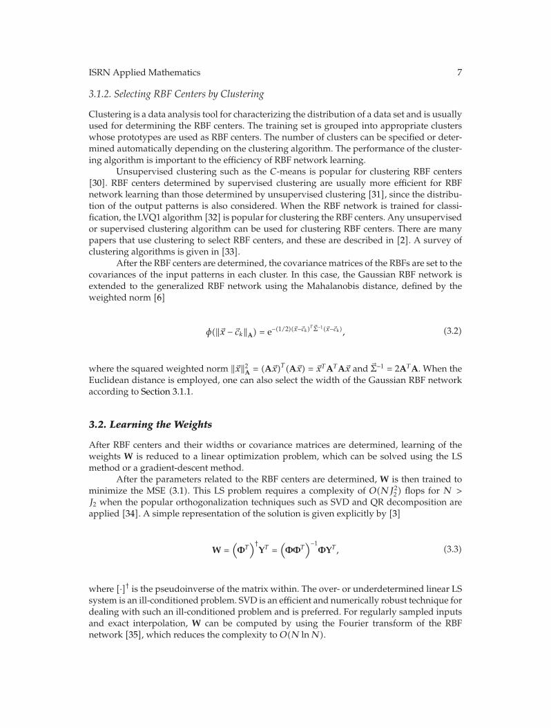
3.1.2. Selecting RBF Centers by Clustering
Clustering is a data analysis tool for characterizing the distribution of a data set and is usuallyused for determining the RBF centers. The training set is grouped into appropriate clusterswhose prototypes are used as RBF centers. The number of clusters can be specified or deter-mined automatically depending on the clustering algorithm. The performance of the cluster-ing algorithm is important to the efficiency of RBF network learning.
Unsupervised clustering such as the C-means is popular for clustering RBF centers[30]. RBF centers determined by supervised clustering are usually more efficient for RBFnetwork learning than those determined by unsupervised clustering [31], since the distribu-tion of the output patterns is also considered. When the RBF network is trained for classi-fication, the LVQ1 algorithm [32] is popular for clustering the RBF centers. Any unsupervisedor supervised clustering algorithm can be used for clustering RBF centers. There are manypapers that use clustering to select RBF centers, and these are described in [2]. A survey ofclustering algorithms is given in [33].
After the RBF centers are determined, the covariance matrices of the RBFs are set to thecovariances of the input patterns in each cluster. In this case, the Gaussian RBF network isextended to the generalized RBF network using the Mahalanobis distance, defined by theweighted norm [6]
φ(‖�x − �ck‖A) = e−(1/2)(�x−�ck)T �Σ−1(�x−�ck), (3.2)
where the squared weighted norm ‖�x‖2A = (A�x)T (A�x) = �xTATA�x and �Σ−1 = 2ATA. When the
Euclidean distance is employed, one can also select the width of the Gaussian RBF networkaccording to Section 3.1.1.
3.2. Learning the Weights
After RBF centers and their widths or covariance matrices are determined, learning of theweights W is reduced to a linear optimization problem, which can be solved using the LSmethod or a gradient-descent method.
After the parameters related to the RBF centers are determined, W is then trained tominimize the MSE (3.1). This LS problem requires a complexity of O(NJ2
2 ) flops for N >J2 when the popular orthogonalization techniques such as SVD and QR decomposition areapplied [34]. A simple representation of the solution is given explicitly by [3]
W =(ΦT)†YT =
(ΦΦT
)−1ΦYT , (3.3)
where [·]† is the pseudoinverse of the matrix within. The over- or underdetermined linear LSsystem is an ill-conditioned problem. SVD is an efficient and numerically robust technique fordealing with such an ill-conditioned problem and is preferred. For regularly sampled inputsand exact interpolation, W can be computed by using the Fourier transform of the RBFnetwork [35], which reduces the complexity to O(N lnN).

8 ISRN Applied Mathematics
When the full data set is not available and samples are obtained on-line, the RLSmethod can be used to train the weights on-line [36]
�wi(t) = �wi(t − 1) + �k(t)ei(t),
�k(t) =P(t − 1)�φt
�φTt P(t − 1)�φt + μ,
ei(t) = yt,i − �φTt �wi(t − 1),
P(t) =1μ
[P(t − 1) − �k(t)�φTt P(t − 1)
],
(3.4)
for i = 1, . . . , J3, where 0 < μ ≤ 1 is the forgetting factor. Typically, P(0) = a0IJ2 , a0 being a suffi-ciently large number and IJ2 the J2×J2 identity matrix, and �wi(0) is selected as a small randommatrix.
In order to eliminate the inversion operation given in (3.3), an efficient, noniterativeweight learning technique has been introduced by applying the Gram-Schmidt orthogonal-ization (GSO) of RBFs [37]. The RBFs are first transformed into a set of orthonormal RBFs forwhich the optimum weights are computed. These weights are then recomputed in such a waythat their values can be fitted back into the original RBF network structure, that is, with kernelfunctions unchanged. The requirement for computing the off-diagonal terms in the solutionof the linear set of weight equations is thus eliminated. In addition, the method has low stor-age requirements since the weights can be computed recursively, and the computation can beorganized in a parallel manner. Incorporation of new hidden nodes does not require recom-putation of the network weights already calculated. This allows for a very efficient networktraining procedure, where network hidden nodes are added one at a time until an adequateerror goal is reached. The contribution of each RBF to the overall network output can beevaluated.
3.3. RBF Network Learning Using Orthogonal Least Squares
The orthogonal least-squares (OLS) method [16, 38, 39] is an efficient way for subset modelselection. The approach chooses and adds RBF centers one by one until an adequate networkis constructed. All the training examples are considered as candidates for the centers, and theone that reduces the MSE the most is selected as a new hidden unit. The GSO is first used toconstruct a set of orthogonal vectors in the space spanned by the vectors of the hidden unitactivation �φp, and a new RBF center is then selected by minimizing the residual MSE. Modelselection criteria are used to determine the size of the network.
The batch OLS method can not only determine the weights, but also choose the num-ber and the positions of the RBF centers. The batch OLS can employ the forward [38–40] andthe backward [41] center selection approaches. When the RBF centers are distinct, ΦT is offull rank. The orthogonal decomposition of ΦT is performed using QR decomposition
ΦT = Q
[R
0
], (3.5)

ISRN Applied Mathematics 9
where Q = [�q1, . . . , �qN] is an N × N orthogonal matrix and R is a J2 × J2 upper triangularmatrix. By minimizing the MSE given by (3.1), one can make use of the invariant property ofthe Frobenius norm
E =1N
∥∥∥QTYT −QTΦTW∥∥∥2
F. (3.6)
Let QTYT =[BB
], where B = [bij] and B = [bij] are, respectively, a J2 × J3 and an (N − J2) × J3
matrix. We then have
E =1N
∥∥∥∥∥[B − RW
B
]∥∥∥∥∥2
F
. (3.7)
Thus, the optimal W is derived from
RW = B. (3.8)
In this case, the residual E = (1/N)‖B‖2F .
Due to the orthogonalization procedure, it is very convenient to implement the for-ward and backward center selection approaches. The forward selection approach is to buildup a network by adding, one at a time, centers at the data points that result in the largestdecrease in the network output error at each stage. Alternatively, the backward selection algo-rithm sequentially removes from the network, one at a time, those centers that cause thesmallest increase in the residual.
The error reduction ratio (ERR) due to the kth RBF neuron is defined by [39]
ERRk =
(∑J3i=1 b
2ki
)�qTk�qk
tr(YYT
) , k = 1, . . . ,N. (3.9)
RBF network training can be in a constructive way, and the centers with the largest ERRvalues are recruited until
1 −J2∑k=1
ERRk < ρ, (3.10)
where ρ ∈ (0, 1) is a tolerance.ERR is a performance-oriented criterion. An alternative terminating criterion can be
based on the Akaike information criterion (AIC) [39, 42], which balances between the perfor-mance and the complexity. The weights are determined at the same time. The criterion usedto stop center selection is a simple threshold on the ERR. If the threshold chose results invery large variances for Gaussian functions, poor generalization performance may occur. Toimprove generalization, regularized forward OLS methods can be implemented by pena-lizing large weights [43, 44]. In [45], the training objective is defined by E +
∑Mi λiw
2i , where
λi’s are the local regularization parameter and M is the number of weights.

10 ISRN Applied Mathematics
The computation complexity of the orthogonal decomposition of ΦT is O(NJ22 ). When
the size of a training data set N is large, the batch OLS is computationally demanding andalso needs a large amount of computer memory.
The RBF center clustering method based on the Fisher ratio class separability measure[46] is similar to the forward selection OLS algorithm [38, 39]. Both the methods employthe QR decomposition-based orthogonal transform to decorrelate the responses of the proto-type neurons as well as the forward center selection procedure. The OLS evaluates candidatecenters based on the approximation error reduction in the context of nonlinear approxima-tion, while the Fisher ratio-based forward selection algorithm evaluates candidate centersusing the Fisher ratio class separability measure for the purpose of classification. The twoalgorithms have similar computational cost.
Recursive OLS (ROLS) algorithms are proposed for updating the weights of single-input single-output [47] and multi-input multioutput systems [48, 49]. In [48], the ROLSalgorithm determines the increment of the weight matrix. In [49], the full weight matrix isdetermined at each iteration, and this reduces the accumulated error in the weight matrix,and the ROLS has been extended for the selection of the RBF centers. After training with theROLS, the final triangular system of equations in a form similar to (3.8) contains importantinformation about the learned network and can be used to sequentially select the centers tominimize the network output error. Forward and backward center selection methods aredeveloped from this information, and Akaike’s FPE criterion [50] is used in the model selec-tion [49]. The ROLS selection algorithms sort the selected centers in the order of their sig-nificance in reducing the MSE [48, 49].
3.4. Supervised Learning of All Parameters
The gradient-descent method provides the simplest solution. We now apply the gradient-descent method to supervised learning of the RBF network.
3.4.1. Supervised Learning for General RBF Networks
To derive the supervised learning algorithm for the RBF network with any useful RBF, werewrite the error function (3.1) as
E =1N
N∑n=1
J3∑i=1
(en,i)2, (3.11)
where en,i is the approximation error at the ith output node for the nth example
en,i = yn,i −J2∑m=1
wmiφ(‖�xn − �cm‖) = yn,i − �wTi�φn. (3.12)
ISRN Applied Mathematics 11
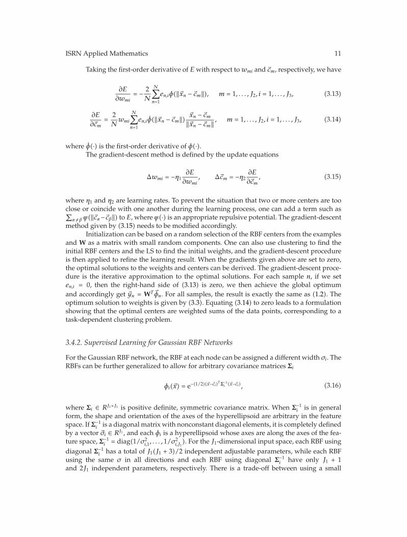
Taking the first-order derivative of E with respect to wmi and �cm, respectively, we have
∂E
∂wmi= − 2
N
N∑n=1
en,iφ(‖�xn − �cm‖), m = 1, . . . , J2, i = 1, . . . , J3, (3.13)
∂E
∂�cm=
2Nwmi
N∑n=1
en,iφ(‖�xn − �cm‖) �xn − �cm‖�xn − �cm‖ , m = 1, . . . , J2, i = 1, . . . , J3, (3.14)
where φ(·) is the first-order derivative of φ(·).The gradient-descent method is defined by the update equations
Δwmi = −η1∂E
∂wmi, Δ�cm = −η2
∂E
∂�cm, (3.15)
where η1 and η2 are learning rates. To prevent the situation that two or more centers are tooclose or coincide with one another during the learning process, one can add a term such as∑
α/= β ψ(‖�cα−�cβ‖) to E, where ψ(·) is an appropriate repulsive potential. The gradient-descentmethod given by (3.15) needs to be modified accordingly.
Initialization can be based on a random selection of the RBF centers from the examplesand W as a matrix with small random components. One can also use clustering to find theinitial RBF centers and the LS to find the initial weights, and the gradient-descent procedureis then applied to refine the learning result. When the gradients given above are set to zero,the optimal solutions to the weights and centers can be derived. The gradient-descent proce-dure is the iterative approximation to the optimal solutions. For each sample n, if we seten,i = 0, then the right-hand side of (3.13) is zero, we then achieve the global optimumand accordingly get �yn = WT �φn. For all samples, the result is exactly the same as (1.2). Theoptimum solution to weights is given by (3.3). Equating (3.14) to zero leads to a formulationshowing that the optimal centers are weighted sums of the data points, corresponding to atask-dependent clustering problem.
3.4.2. Supervised Learning for Gaussian RBF Networks
For the Gaussian RBF network, the RBF at each node can be assigned a different width σi. TheRBFs can be further generalized to allow for arbitrary covariance matrices Σi
φi(�x) = e−(1/2)(�x−�ci)TΣ−1i (�x−�ci), (3.16)
where Σi ∈ RJ1×J1 is positive definite, symmetric covariance matrix. When Σ−1i is in general
form, the shape and orientation of the axes of the hyperellipsoid are arbitrary in the featurespace. If Σ−1
i is a diagonal matrix with nonconstant diagonal elements, it is completely definedby a vector �σi ∈ RJ1 , and each φi is a hyperellipsoid whose axes are along the axes of the fea-ture space, Σ−1
i = diag(1/σ2i,1, . . . , 1/σ
2i,J1
). For the J1-dimensional input space, each RBF usingdiagonal Σ−1
i has a total of J1(J1 + 3)/2 independent adjustable parameters, while each RBFusing the same σ in all directions and each RBF using diagonal Σ−1
i have only J1 + 1and 2J1 independent parameters, respectively. There is a trade-off between using a small

12 ISRN Applied Mathematics
network with many adjustable parameters and using a large network with fewer adjustableparameters.
When using the RBF using the same σ in all directions, we get the gradients as
∂E
∂�cm= − 2
N
N∑n=1φm(�xn)
�xn − �cmσ2m
J3∑i=1en,iwi,m,
∂E
∂σm= − 2
N
N∑n=1φm(�xn)
‖�xn − �cm‖2
σ3m
J3∑i=1en,iwi,m.
(3.17)
Similarly, for the RBF using diagonal Σ−1i , the gradients are given by
∂E
∂cm,j= − 2
N
N∑n=1φm(�xn)
xn,j − cm,jσ2m,j
J3∑i=1en,iwi,m,
∂E
∂σm,j= − 2
N
N∑n=1φm(�xn)
(xn,j − cm,j
)2
σ3m,j
J3∑i=1en,iwi,m.
(3.18)
Adaptations for �ci and Σi are along the negative gradient directions. W are updated by (3.13)and (3.15). To prevent unreasonable radii, the updating algorithms can also be derived byadding to the MSE E a constraint term that penalizes small radii, Ec =
∑i 1/σi or Ec =∑
i,j 1/σi,j .
3.4.3. Remarks
The gradient-descent algorithms introduced so far are batch learning algorithms. By opti-mizing the error function Ep for each example (�xp, �yp), one can update the parameters in theincremental learning model, which are typically much faster than their batch counterparts forsuitably selected learning parameters.
Although the RBF network trained by the gradient-descent method is capable of pro-viding equivalent or better performance compared to that of the MLP trained with the BP, thetraining time for the two methods are comparable [51]. The gradient-descent method is slowin convergence since it cannot efficiently use the locally tuned representation of the hidden-layer units. When the hidden-unit receptive fields, controlled by the widths σi, are narrow, fora given input only a few of the total number of hidden units will be activated and hence onlythese units need to be updated. However, the gradient-descent method may leads to largewidth, and then the original idea of using a number of local tuning units to approximatethe target function cannot be maintained. Besides, the computational advantage of localitycannot be utilized anymore [30].
The gradient-descent method is prone to finding local minima of the error function.For reasonably well-localized RBF, an input will generate a significant activation in a smallregion, and the opportunity of getting stuck at a local minimum is small. Unsupervised meth-ods can be used to determine σi. Unsupervised learning is used to initialize the network para-meters, and supervised learning is usually used for fine-tuning the network parameters. Theultimate RBF network learning algorithm is typically a blend of unsupervised and supervisedalgorithms. Usually, the centers are selected by using a random subset of the training set or
ISRN Applied Mathematics 13
obtained by using clustering, the variances are selected using a heuristic, and the weights aresolved by using a linear LS method or the gradient-descent method. This combination mayyield a fast learning procedure with a sufficient accuracy.
3.5. Other Learning Methods
Actually, all general-purpose unconstrained optimization methods are applicable for RBFnetwork learning by minimization of E, with no or very little modification. These includepopular second-order approaches like the Levenberg-Marquardt (LM), conjugate gradient,BFGS, and extended Kalman filtering (EKF), and heuristic-based global optimization meth-ods like evolutionary algorithms, simulated annealing, and Tabu search. These algorithmsare described in detail in [2].
The objective is to find suitable network structure and the corresponding networkparameters. Some complexity criteria such as the AIC [42] are used to control a trade-off bet-ween the learning error and network complexity. Heuristic-based global optimization isalso widely used for neural network learning. The selection of the network structure andparameters can be performed simultaneously or separately. For implementation using evolu-tionary algorithm, the parameters associated with each node are usually coded together inthe chromosomes. Some heuristic-based RBF network learning algorithms are described in[2].
The LM method is used for RBF network learning [52–54]. In [53, 54], the LM methodis used for estimating nonlinear parameters, and the LS method is used for weight estimationat each iteration. All model parameters are optimized simultaneously. In [54], at each iterationthe weights are updated many times during the process of looking for the search directionto update the nonlinear parameters. This further accelerates the convergence of the searchprocess. RBF network learning can be viewed as a system identification problem. After thenumber of centers is chosen, the EKF simultaneously solves for the prototype vectors andthe weight matrix [55]. A decoupled EKF further decreases the complexity of the trainingalgorithm [55]. EKF training provides almost the same performance as gradient-descenttraining, but with only a fraction of the computational cost. In [56], a pair of parallel runningextended Kalman filters are used to sequentially update both the output weights and the RBFcenters.
In [57], BP with selective training [58] is applied to RBF network learning. The methodimproves the performance of the RBF network substantially compared to the gradient-des-cent method, in terms of convergence speed and accuracy. The method is quite effective whenthe dataset is error-free and nonoverlapping. In [15], the RBF network is reformulated byusing RBFs formed in terms of admissible generator functions and provides a fully super-vised gradient-descent training method. A learning algorithm is proposed in [59] for traininga special class of reformulated RBF networks, known as cosine RBF networks. It trainsreformulated RBF networks by updating selected adjustable parameters to minimize theclass-conditional variances at the outputs of their RBFs so as to be capable of identifying un-certainty in data classification.
Linear programming models with polynomial time complexity are also employed totrain the RBF network [60]. A multiplication-free Gaussian RBF network with a gradient-based nonlinear learning algorithm [61] is described for adaptive function approximation.
The expectation-maximization (EM) method [62] is an efficient maximum likelihood-based method for parameter estimation; it splits a complex problem into many separatesmall-scale subproblems. The EM method has also been applied for RBF network learning

14 ISRN Applied Mathematics
[63–65]. The shadow targets algorithm [66], which employs a philosophy similar to that of theEM method, is an efficient RBF network training algorithm for topographic feature extraction.
The RBF network using regression weights can significantly reduce the number ofhidden units and is effectively used for approximating nonlinear dynamic systems [22, 25,64]. For a J1-J2-1 RBF network, the weight from the ith hidden unit to the output unit wi isdefined by the linear regression [64] wi = �aTi �x + ξi, where �ai = (ai,0, ai,1, . . . , ai,J1)
T is the reg-ression parameter vector, �x = (1,x1, . . . ,xJ1)
T is the augmented input vector, and ξi is zero-mean Gaussian noise. For the Gaussian RBF network, the RBF centers �ci and their widths σican be selected by the C-means and the nearest-neighbor heuristic, while the parameters ofthe regression weights are estimated by the EM method [64]. The RBF network with linearregression weights has also been studied [25], where a simple but fast computational pro-cedure is achieved by using a high-dimensional raised-cosine RBF.
When approximating a given function f(x), a parsimonious design of the GaussianRBF network can be achieved based on the Gaussian spectrum of f(x), γG(f ; �c, σ) [67].According to the Gaussian spectrum, one can estimate the necessary number of RBF unitsand evaluate how appropriate the use of the Gaussian RBF network is. Gaussian RBFs areselected according to the peaks (negative as well as positive) of the Gaussian spectrum. Onlythe weights of the RBF network are needed to be tuned. Analogous to principal componentanalysis (PCA) of the data sets, the principal Gaussian components of f(x) are extracted. Ifthere are a few sharp peaks on the spectrum surface, the Gaussian RBF network is suitablefor approximation with a parsimonious architecture. However, if there are many peaks withsimilar importance or small peaks situated in large flat regions, this method will be inefficient.
The Gaussian RBF network can be regarded as an improved alternative to the four-layer probabilistic neural network (PNN) [68]. In a PNN, a Gaussian RBF node is placed atthe position of each training pattern so that the unknown density can be well interpolated andapproximated. This technique yields optimal decision surfaces in the Bayes’ sense. Training isto associate each node with its target class. This approach, however, severely suffers from thecurse of dimensionality and results in a poor generalization. The probabilistic RBF network[69] constitutes a probabilistic version of the RBF network for classification that extends thetypical mixture model approach to classification by allowing the sharing of mixture compo-nents among all classes. The probabilistic RBF network is an alternative approach for class-conditional density estimation. It provides output values corresponding to the class-con-ditional densities p(�x | k) (for class k). The typical learning method of probabilistic RBFnetwork for a classification task employs the EM algorithm, which highly depends on theinitial parameter values. In [70], a technique for incremental training of the probabilistic RBFnetwork for classification is proposed, based on criteria for detecting a region that is crucialfor the classification task. After the addition of all components, the algorithm splits everycomponent of the network into subcomponents, each one corresponding to a different class.
Extreme learning machine (ELM) [71] is a learning algorithm for single-hidden layerfeedforward neural networks (SLFNs). ELM in an incremental method (I-ELM) is proved tobe a universal approximator [17]. It randomly chooses hidden nodes and analytically deter-mines the output weights of SLFNs. In theory, this algorithm tends to provide good general-ization performance at extremely fast learning speed, compared to gradient-based algorithmsand SVM. ELM is a simple and efficient three-step learning method, which does not requireBP or iterative techniques. ELM can analytically determine all the parameters of SLFNs.Unlike the gradient-based algorithms, the ELM algorithm could be used to train SLFNswith many nondifferentiable activation functions (such as the threshold function) [72].

ISRN Applied Mathematics 15
Theoretically the ELM algorithm can be used to train neural networks with threshold func-tions directly instead of approximating them with sigmoid functions [72]. In [73], an onlinesequential ELM (OS-ELM) algorithm is developed to learn data one by one or chunk bychunk with fixed or varying chunk size. In OS-ELM, the parameters of hidden nodes arerandomly selected, and the output weights are analytically determined based on the sequ-entially arriving data. Apart from selecting the number of hidden nodes, no other controlparameters have to be manually chosen.
4. Optimizing Network Structure
In order to achieve the optimum structure of an RBF network, learning can be performed bydetermining the number and locations of the RBF centers automatically using constructiveand pruning methods.
4.1. Constructive Approach
The constructive approach gradually increases the number of RBF centers until a criterion issatisfied. The forward OLS algorithm [16] described in Section 3.3 is a well-known construc-tive algorithm. Based on the OLS algorithm, a constructive algorithm for the generalizedGaussian RBF network is given in [74]. RBF network learning based on a modification tothe cascade-correlation algorithm [75] works in a way similar to the OLS method, but witha significantly faster convergence [76]. The OLS incorporated with the sensitivity analysis isalso employed to search for the optimal RBF centers [77]. A review on constructive appro-aches to structural learning of feedforward networks is given in [78].
In [79], a new prototype is created in a region of the input space by splitting an existingprototype �cj selected by a splitting criterion, and splitting is performed by adding the per-turbation vectors ±�εj to �cj . The resulting vectors �cj ±�εj together with the existing centers formthe initial set of centers for the next growing cycle. �εj can be obtained by a deviation measurecomputed from �cj and the input vectors represented by �cj , and ‖�εj‖ ‖�cj‖. Feedback splittingand purity splitting are two criteria for the selection of splitting centers. Existing algorithmsfor updating the centers �cj , widths σj , and weights can be used. The process continues untila stopping criterion is satisfied.
In a heuristic incremental algorithm [80], the training phase is an iterative process thatadds a hidden node �ct at each epoch t by an error-driven rule. Each epoch t consists of threephases. The data point with the worst approximation, denoted �xs, is first recruited as a newhidden node �ct = �xs, and its weight to each output node j, wtj , is fixed at the error at the jthoutput node performed by the network at the (t − 1)th epoch on �xs. The next two phases are,respectively, local tuning and fine tuning of the variances of the RBFs.
The incremental RBF network architecture using hierarchical gridding of the inputspace [81] allows for a uniform approximation without wasting resources. The centers andvariances of the added nodes are fixed through heuristic considerations. Additional layersof Gaussians at lower scales are added where the residual error is higher. The number ofGaussians of each layer and their variances are computed from considerations based onlinear filtering theory. The weight of each Gaussian is estimated through a maximum a pos-teriori estimate carried out locally on a subset of the data points. The method shows a highaccuracy in the reconstruction, and it can deal with nonevenly spaced data points and isfully parallelizable. Similarly, the hierarchical RBF network [82] is a multiscale version of the
16 ISRN Applied Mathematics
RBF network. It is constituted by hierarchical layers, each containing a Gaussian grid at adecreasing scale. The grids are not completely filled, but units are inserted only where thelocal error is over a threshold. The constructive approach is based only on the local opera-tions, which do not require any iteration on the data. Like traditional wavelet-based multi-resolution analysis (MRA), the hierarchical RBF network employs Riesz bases and enjoysasymptotic approximation properties for a very large class of functions.
The dynamic decay adjustment (DDA) algorithm is a fast constructive trainingmethod for the RBF network when used for classification [83]. It is motivated from the pro-babilistic nature of the PNN [68], the constructive nature of the restricted Coulomb energy(RCE) networks [84] as well as the independent adjustment of the decay factor or width σi ofeach prototype. The DDA method is faster and also achieves a higher classification accuracythan the conventional RBF network [30], the MLP trained with the Rprop, and the RCE.
Incremental RBF network learning is also derived based on the growing cell structuresmodel [85] and based on a Hebbian learning rule adapted from the neural gas model [86].The insertion strategy is on accumulated error of a subset of the data set. Another example ofthe constructive approach is the competitive RBF algorithm based on maximum-likelihoodclassification [87]. The resource-allocating network (RAN) [88] is a well-known RBF networkconstruction method [88] and is introduced in Section 4.2.
4.2. Resource-Allocating Networks
The RAN is a sequential learning method for the localized RBF network, which is suitable foronline modeling of nonstationary processes. The network begins with no hidden units. As thepattern pairs are received during the training, a new hidden unit may be recruited accordingto the novelty in the data. The novelty in the data is decided by two conditions
‖�xt − �ci‖ > ε(t), (4.1)
‖�e(t)‖ =∥∥�yt − f(�xt)∥∥ > emin, (4.2)
where �ci is the center nearest to �xt, the prediction error �e = (e1, . . . , eJ3)T , and ε(t) and emin are
two thresholds. The algorithm starts with ε(t) = εmax, where εmax is chosen as the largest scalein the input space, typically the entire input space of nonzero probability. ε(t) shrinks expo-nentially by ε(t) = max{εmaxe−t/τ , εmin}, where τ is a decay constant. ε(t) is decayed until itreaches εmin.
Assuming that there are k nodes at time t−1, for the Gaussian RBF network, the newlyadded hidden unit at time t can be initialized as
�ck+1 = �xt,
w(k+1)j = ej(t), j = 1, . . . , J3,
σk+1 = α‖�xt − �ci‖,(4.3)
where the value for σk+1 is based on the nearest-neighbor heuristic and α is a parameter defin-ing the size of neighborhood. If a pattern pair (�xt, �yt) does not pass the novelty criteria, nohidden unit is added and the existing network parameters are adapted using the LMS method[89].

ISRN Applied Mathematics 17
The RAN method performs much better than the RBF network learning algorithmusing random centers and that using the centers clustered by theC-means [30] in terms of net-work size and MSE. The RAN method achieves roughly the same performance as the MLPtrained with the BP, but with much less computation.
In [90], an agglomerative clustering algorithm is used for RAN initialization, insteadof starting from zero hidden node. In [91], the LMS method is replaced by the EKF method forthe network parameter adaptation so as to generate a more parsimonious network. Two geo-metric criteria, namely, the prediction error criterion, which is the same as (4.2), and the anglecriterion are also obtained from a geometric viewpoint. The angle criterion assigns RBFs thatare nearly orthogonal to all the other existing RBFs. These criteria are proved to be equivalentto Platt’s criteria [88]. In [92], the statistical novelty criterion is defined by using the resultof the EKF method. By using the EKF method and using this criterion to replace the criteria(4.1) and (4.2), more compact networks and smaller MSEs are achieved than the RAN [88]and the EKF-based RAN [91].
Numerous improvements on the RAN have been made by integrating node-pruningprocedure [93–99]. The minimal RAN [93, 94] is based on the EKF-based RAN [91] and achi-eves a more compact network with equivalent or better accuracy by incorporating a pruningstrategy to remove inactive nodes and augmenting the basic growth criterion of the RAN.The output of each RBF unit is linearly scaled to oi(�x) ∈ (0, 1]. If oi(�x) is below a predefinedthreshold δ for a given number of iterations, this node is idle and can be removed. For a givenaccuracy, the minimal RAN achieves a smaller complexity than the MLP trained with RProp[100]. In [95], the RAN is improved by using Givens QR decomposition-based RLS for theadaptation of the weights and integrating a node-pruning strategy. The ERR criterion in [38]is used to select the most important regressors. In [96], the RAN is improved by using ineach iteration the combination of the SVD and QR-cp methods for determining the structureas well as for pruning the network. In the early phase of learning, the addition of RBFs is insmall groups, and this leads to an increased rate of convergence. If a particular RBF is not con-sidered for a given number of iterations, it is removed. The size of the network is more com-pact than the RAN.
In [97], the EKF and statistical novelty criterion-based method [92] is extended byincorporating an online pruning procedure, which is derived using the parameters andinnovation statistics estimated from the EKF. The online pruning method is analogous to thesaliency-based optimal brain surgeon (OBS) [101] and optimal brain damage (OBD) [102].The IncNet and IncNet Pro [103] are RAN-EKF networks with statistically controlled growthcriterion. The pruning method is similar to the OBS, but based on the result of the EKF algo-rithm.
The growing and pruning algorithm for RBF (GAP-RBF) [98] and the generalizedGAP-RBF (GGAP-RBF) [99] are RAN-based sequential learning algorithms. These algo-rithms make use of the notion of significance of a hidden neuron, which is defined as aneuron’s statistical contribution over all the inputs seen so far to the overall performance ofthe network. In addition to the two growing criteria of the RAN, a new neuron is added onlywhen its significance is also above a chosen learning accuracy. If during the training the signi-ficance of a neuron becomes less than the learning accuracy, that neuron will be pruned. Foreach new pattern, only its nearest neuron is checked for growing, pruning, or updating usingthe EKF. The GGAP-RBF enhances the significance criterion such that it is applicable fortraining samples with arbitrary sampling density. Both the GAP-RBF and the GGAP-RBF out-perform the RAN [88], the EKF-based RAN [91], and the minimal RAN [94] in terms of learn-ing speed, network size, and generalization performance.
18 ISRN Applied Mathematics
4.3. Constructive Methods with Pruning
In addition to the RAN algorithms with pruning strategy [93–99], there are some other cons-tructive methods with pruning.
The normalized RBF network [22] can be sequentially constructed with pruning strat-egy based on the novelty of the data and the overall behaviour of the network using thegradient-descent method. The network starts from one neuron and adds a new neuron if anexample passes two novelty criteria. The first criterion is the same as (4.2), and the second onedeals with the activation of the nonlinear neurons, maxi φi(�xt) < ζ, where ζ is a threshold. Thepseudo-Gaussian RBF is used, and RBF weights are linear regression functions of the inputvariables. After the whole pattern set is presented at an epoch, the algorithm starts to removethose neurons that meet any of the three cases, namely, neurons with a very small meanactivation for the whole pattern set, neurons with a very small activation region, or neuronshaving an activation very similar to that of other neurons.
In [104], training starts with zero hidden node and progressively builds the model asnew data become available. A fuzzy partition of the input space defines a multidimensionalgrid, from which the RBF centers are selected, so that at least one selected RBF center is closeenough to each input example. The method is capable of adapting on-line the structure of theRBF network, by adding new units when an input example does not belong to any of the sub-spaces that have been selected, or deleting old ones when no data have been assigned to therespective fuzzy subspaces for a long period of time. The weights are updated using the RLSalgorithm. The method avoids selecting the centers only among the available data.
As an efficient and fast growing RBF network algorithm, the constructive nature ofDDA [83] may result in too many neurons. The DDA with temporary neurons improves theDDA by introducing online pruning of neurons after each DDA training epoch [105]. Aftereach training epoch, if the individual neurons cover a sufficient number of samples, they aremarked as permanent; otherwise, they are deleted. This mechanism results in a significantreduction in the number of neurons. The DDA with selective pruning and model selection isanother extension to the DDA [106], where only a portion of the neurons which cover onlyone training sample are pruned and pruning is carried out only after the last epoch of theDDA training. The method improves the generalization performance of the DDA [83] andthe DDA with temporary neurons [105], but yields a larger network size than the DDA withtemporary neurons. The pruning strategy proposed in [107] aims to detect and remove thoseneurons to improve generalization. When the dot product values of two nodes is beyond athreshold, one of the two nodes can be pruned.
4.4. Pruning Methods
Various pruning methods for feedforward networks have been discussed in [2]. These meth-ods are applicable to the RBF network since the RBF network is a kind of feedforward net-work. Well-known pruning methods are the weight-decay technique [43, 45], the OBD [102],and OBS [101]. Pruning algorithms based on the regularization technique are also popularsince additional terms that penalize the complexity of the network are incorporated into theMSE criterion.
With the flavor of weight-decay technique, some regularization techniques for improv-ing the generalization capability of the MLP and the RBF network are also discussed in [108].As in the MLP, the favored penalty term
∑w2ij is also appropriate for the RBF network. The
ISRN Applied Mathematics 19
widths of the RBFs is a major source of ill-conditioning in RBF network learning, and largewidth parameters are desirable for better generalization. Some suitable penalty terms forwidths are given in [108]. Fault-tolerance ability of RBF networks are also described based ona regularization technique. In [109], a Kullback-Leibler divergence-based objective functionis defined for improving the fault-tolerance of RBF networks. The learning method achieves abetter fault-tolerant ability, compared with weight-decay-based regularizers. In [110], a regu-larization-based objective function for training a functional link network to tolerate multi-plicative weight noise is defined, and a simple learning algorithm is derived. The functionlink network is somewhat similar to the RBF network. Under some mild conditions the deri-ved regularizer is essentially the same as a weight decay regularizer. This explains why apply-ing weight decay can also improve the fault-tolerant ability of an RBF with multiplicativeweight noise.
In [111], the pruning method starts from a large RBF network and achieves a compactnetwork through an iterative procedure of training and selection. The training procedureadaptively changes the centers and the width of the RBFs and trains the linear weights. Theselection procedure performs the elimination of the redundant RBFs using an objective func-tion based on the MDL principle [112]. In [113], all the data vectors are initially selected ascenters. Redundant centers in the RBF network are eliminated by merging two centers at eachadaptation cycle by using an iterative clustering method. The technique is superior to thetraditional RBF network algorithms, particularly in terms of the processing speed and solva-bility of nonlinear patterns.
4.5. Model Selection
A theoretically well-motivated criterion for describing the generalization error is developedby using Stein’s unbiased risk estimator (SURE) [114]
Err(J2) = err(J2) −Nσ2n + 2σ2
n(J2 + 1), (4.4)
where Err is the generalization error on the new data, err denotes the training error for eachmodel, J2 is the number of RBF nodes, N is the size of the pattern set, and σ2
n is the noise vari-ance, which can be estimated from the MSE of the model. An empirical comparison amongthe SURE-based method, cross-validation, and the Bayesian information criterion (BIC)[115], is made in [114]. The generalization error of the models by the SURE-based methodcan be less than that of the models selected by cross-validation, but with much less computa-tion. The SURE-based method has a behavior similar to the BIC. However, the BIC generallygives preference to simpler models since it penalizes complex models more harshly.
The generalization error of a trained network can be decomposed into two parts,namely, an approximation error that is due to the finite number of parameters of the approxi-mation scheme and an estimation error that is due to the finite number of data available [116,117]. For a feedforward network with J1 input nodes and a single output node, a bound forthe generalization error is given by [116, 117]
O
(1P
)+O
([PJ1 ln(PN) − ln δ
N
]1/2), (4.5)
20 ISRN Applied Mathematics
with a probability greater than 1 − δ, where N is the number of examples, δ ∈ (0, 1) is theconfidence parameter, and P is proportional to the number of parameters such as P hiddenunits in an RBF network. The first term in (4.5) corresponds to the bound on the approxi-mation error, and the second on the estimation error. As P increases, the approximation errordecreases since we are using a larger model; however, the estimation error increases dueto overfitting (or alternatively, more data). The trade-off between the approximation andestimation errors is best maintained when P is selected as P ∝ N1/3 [116]. After suitablyselecting P and N, the generalization error for feedforward networks should be O(1/P).This result is similar to that for an MLP with sigmoidal functions [118]. The bound given by(4.5) has been considerably improved to O((lnN/N)1/2) in [119] for RBF network learningwith the MSE function.
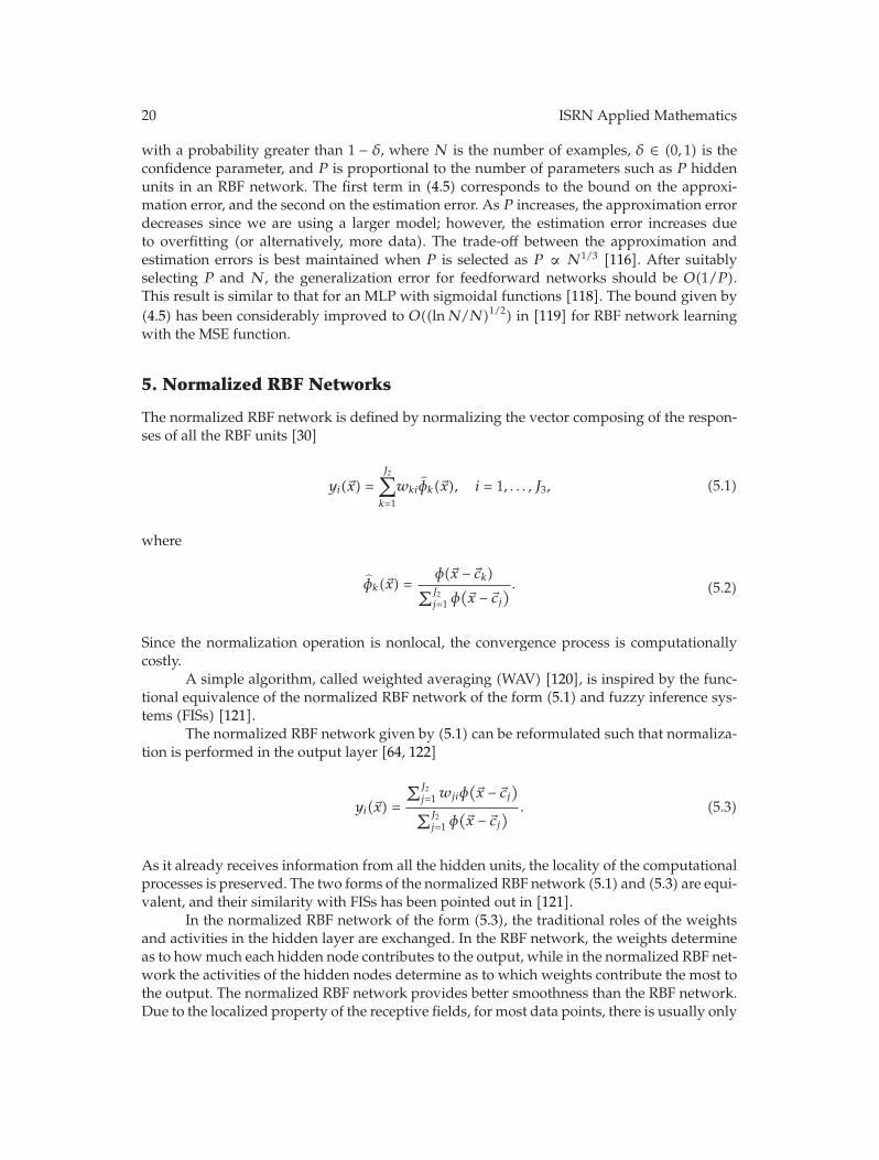
5. Normalized RBF Networks
The normalized RBF network is defined by normalizing the vector composing of the respon-ses of all the RBF units [30]
yi(�x) =J2∑k=1
wkiφk(�x), i = 1, . . . , J3, (5.1)
where
φk(�x) =φ(�x − �ck)∑J2j=1 φ
(�x − �cj
) . (5.2)
Since the normalization operation is nonlocal, the convergence process is computationallycostly.
A simple algorithm, called weighted averaging (WAV) [120], is inspired by the func-tional equivalence of the normalized RBF network of the form (5.1) and fuzzy inference sys-tems (FISs) [121].
The normalized RBF network given by (5.1) can be reformulated such that normaliza-tion is performed in the output layer [64, 122]
yi(�x) =
∑J2j=1 wjiφ
(�x − �cj
)∑J2
j=1 φ(�x − �cj
) . (5.3)
As it already receives information from all the hidden units, the locality of the computationalprocesses is preserved. The two forms of the normalized RBF network (5.1) and (5.3) are equi-valent, and their similarity with FISs has been pointed out in [121].
In the normalized RBF network of the form (5.3), the traditional roles of the weightsand activities in the hidden layer are exchanged. In the RBF network, the weights determineas to how much each hidden node contributes to the output, while in the normalized RBF net-work the activities of the hidden nodes determine as to which weights contribute the most tothe output. The normalized RBF network provides better smoothness than the RBF network.Due to the localized property of the receptive fields, for most data points, there is usually only

ISRN Applied Mathematics 21
one hidden node that contributes significantly to (5.3). The normalized RBF network can betrained using a procedure similar to that for the RBF network. The normalized Gaussian RBFnetwork exhibits superiority in supervised classification due to its soft modification rule[123]. It is also a universal approximator in the space of continuous functions with compactsupport in the space Lp(Rp, d�x) [124].
The normalized RBF network loses the localized characteristics of the localized RBFnetwork and exhibits excellent generalization properties, to the extent that hidden nodes needto be recruited only for training data at the boundaries of the class domains. This obviates theneed for a dense coverage of the class domains, in contrast to the RBF network. Thus, the nor-malized RBF network softens the curse of dimensionality associated with the localized RBFnetwork [122]. The normalized Gaussian RBF network outperforms the Gaussian RBF net-work in terms of the training and generalization errors, exhibits a more uniform error overthe training domain, and is not sensitive to the RBF widths.
The normalized RBF network is an RBF network with a quasilinear activation functionwith a squashing coefficient decided by the actviations of all the hidden units. The outputunits can also employ the sigmoidal activation function. The RBF network with the sigmoidalfunction at the output nodes outperforms the case of linear or quasilinear function at the out-put nodes in terms of sensitivity to learning parameters, convergence speed as well asaccuracy [57].
The normalized RBF network is found functionally equivalent to a class of Takagi-Sugeno-Kang (TSK) systems [121]. According to the output of the normalized RBF networkgiven by (5.3), when the t-norm in the TSK model is selected as algebraic product and themembership functions (MFs) are selected the same as RBFs of the RBF network, the twomodels are mathematically equivalent [121, 125]. Note that each hidden unit corresponds to afuzzy rule. In the normalized RBF network, wij ’s typically take constant values; thus the nor-malized RBF network corresponds to the zero-order TSK model. When the RBF weights arelinear regression functions of the input variables [22, 64], the model is functionally equivalentto the first-order TSK model.
6. Applications of RBF Networks
Tradionally, RBF networks are used for function approximation and classification. They aretrained to approximate a nonlinear function, and the trained RBF networks are then used togeneralize. All applications of the RBF network are based on its universal approximationcapability.
RBF networks have now used in a vast variety of applications, such as face trackingand face recognition [126], robotic control [127], antenna design [128], channel equalizations[129, 130], computer vision and graphics [131–133], and solving partial differential equationswith boundary conditions (Dirichlet or Neumann) [134].
Special RBFs are customized to match the data characteristics of some problems. Forinstance, in channel equalization [129, 130], the received signal is complex-valued, and hencecomplex-valued RBFs are considered.
6.1. Vision Applications
In the graphics or vision applications, the input domain is spherical. Hence, the sphericalRBFs [131–133, 135–137] are required.
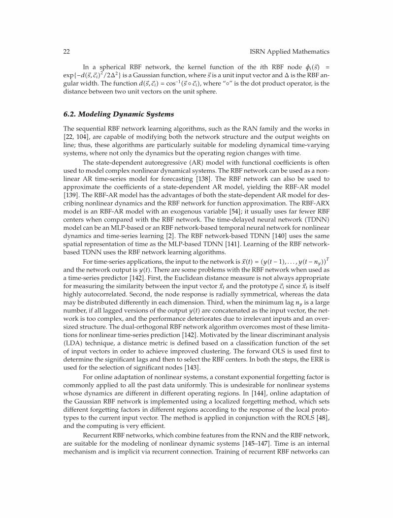
22 ISRN Applied Mathematics
In a spherical RBF network, the kernel function of the ith RBF node φi(�s) =exp{−d(�s, �ci)2/2Δ2} is a Gaussian function, where �s is a unit input vector and Δ is the RBF an-gular width. The function d(�s, �ci) = cos−1(�s ◦ �ci), where “◦” is the dot product operator, is thedistance between two unit vectors on the unit sphere.
6.2. Modeling Dynamic Systems
The sequential RBF network learning algorithms, such as the RAN family and the works in[22, 104], are capable of modifying both the network structure and the output weights online; thus, these algorithms are particularly suitable for modeling dynamical time-varyingsystems, where not only the dynamics but the operating region changes with time.
The state-dependent autoregressive (AR) model with functional coefficients is oftenused to model complex nonlinear dynamical systems. The RBF network can be used as a non-linear AR time-series model for forecasting [138]. The RBF network can also be used toapproximate the coefficients of a state-dependent AR model, yielding the RBF-AR model[139]. The RBF-AR model has the advantages of both the state-dependent AR model for des-cribing nonlinear dynamics and the RBF network for function approximation. The RBF-ARXmodel is an RBF-AR model with an exogenous variable [54]; it usually uses far fewer RBFcenters when compared with the RBF network. The time-delayed neural network (TDNN)model can be an MLP-based or an RBF network-based temporal neural network for nonlineardynamics and time-series learning [2]. The RBF network-based TDNN [140] uses the samespatial representation of time as the MLP-based TDNN [141]. Learning of the RBF network-based TDNN uses the RBF network learning algorithms.
For time-series applications, the input to the network is �x(t) = (y(t − 1), . . . ,y(t − ny))Tand the network output is y(t). There are some problems with the RBF network when used asa time-series predictor [142]. First, the Euclidean distance measure is not always appropriatefor measuring the similarity between the input vector �xt and the prototype �ci since �xt is itselfhighly autocorrelated. Second, the node response is radially symmetrical, whereas the datamay be distributed differently in each dimension. Third, when the minimum lag ny is a largenumber, if all lagged versions of the output y(t) are concatenated as the input vector, the net-work is too complex, and the performance deteriorates due to irrelevant inputs and an over-sized structure. The dual-orthogonal RBF network algorithm overcomes most of these limita-tions for nonlinear time-series prediction [142]. Motivated by the linear discriminant analysis(LDA) technique, a distance metric is defined based on a classification function of the setof input vectors in order to achieve improved clustering. The forward OLS is used first todetermine the significant lags and then to select the RBF centers. In both the steps, the ERR isused for the selection of significant nodes [143].
For online adaptation of nonlinear systems, a constant exponential forgetting factor iscommonly applied to all the past data uniformly. This is undesirable for nonlinear systemswhose dynamics are different in different operating regions. In [144], online adaptation ofthe Gaussian RBF network is implemented using a localized forgetting method, which setsdifferent forgetting factors in different regions according to the response of the local proto-types to the current input vector. The method is applied in conjunction with the ROLS [48],and the computing is very efficient.
Recurrent RBF networks, which combine features from the RNN and the RBF network,are suitable for the modeling of nonlinear dynamic systems [145–147]. Time is an internalmechanism and is implicit via recurrent connection. Training of recurrent RBF networks can

ISRN Applied Mathematics 23
be based on the RCE algorithm [147], gradient descent, or the EKF [146]. Some techniquesfor injecting finite state automata into the network have also been proposed in [145].
6.3. Complex RBF Networks
Complex RBF networks are more efficient than the RBF network, in the case of nonlinear sig-nal processing involving complex-valued signals, such as equalization and modeling of non-linear channels in communication systems. Digital channel equalization can be treated as aclassification problem.
In the complex RBF network [130], the input, the output, and the output weights arecomplex values, whereas the activation function of the hidden nodes is the same as that forthe RBF network. The Euclidean distance in the complex domain is defined by [130]
d(�xt, �ci) =[(�xt − �ci)H(�xt − �ci)
]1/2, (6.1)
where �ci is a J1-dimensional complex center vector. The Mahalanobis distance (3.16) definedfor the Gaussian RBF can be extended to the complex domain [148] by changing the trans-pose T in (3.16) into the Hermitian transpose H. Most existing RBF network learning algo-rithms can be easily extended for training various versions of the complex RBF network [129,130, 148, 149]. When using clustering techniques to determine the RBF centers, the similaritymeasure can be based on the distance defined by (6.1). The Gaussian RBF is usually used inthe complex RBF network. In [129], the minimal RAN algorithm [93] is extended to its com-plex-valued version.
Although the input and centers of the complex RBF network [129, 130, 148, 149] arecomplex valued, each RBF node has a real-valued response that can be interpreted as a con-ditional probability density function. This interpretation makes such a network particularlyuseful in the equalization application of communication channels with complex-valuedsignals. This complex RBF network is essentially two separate real-valued RBF networks.
Learning of the complex Gaussian RBF network can be performed in two phases,where the RBF centers are first selected by using the incremental C-means algorithm [33] andthe weights are then solved by fixing the RBF parameters [148]. At each iteration t, the C-means first finds the winning node with index w by using the nearest-neighbor rule and thenupdates both the center and the variance of the winning node by
�cw(t) = �cw(t − 1) + η[�xt − �cw(t − 1)],
Σw(t) = Σw(t − 1) + η[�xt − �cw(t − 1)][�xt − �cw(t − 1)]H,(6.2)
where η is the learning rate. The C-means is repeated until the changes in all �ci(t) and Σi(t)are within a specified accuracy. After complex RBF centers are determined, the weight matrixW is determined using the LS or RLS algorithm.
In [150], the ELM algorithm is extended to the complex domain, yielding the fullycomplex ELM (C-ELM). For channel equalization, the C-ELM algorithm significantly out-performs the complex minimal RAN [129], complex RBF network [149], and complex back-propagation, in terms of symbol error rate (SER) and learning speed. In [151], a fully com-plex-valued RBF network is proposed for regression and classification applications, which is

24 ISRN Applied Mathematics
based on the locally regularised OLS (LROLS) algorithm aided with the D-optimality expe-rimental design. These models [150, 151] have a complex-valued response at each RBF node.
7. RBF Networks versus MLPs
Both the MLP and the RBF networks are used for supervised learning. In the RBF network,the activation of an RBF unit is determined by the distance between the input vector and theprototype vector. For classification problems, RBF units map input patterns from a nonlinearseparable space to a linear separable space, and the responses of the RBF units form newfeature vectors. Each RBF prototype is a cluster serving mainly a certain class. When the MLPwith a linear output layer is applied to classification problems, minimizing the error at theoutput of the network is equivalent to maximizing the so-called network discriminant func-tion at the output of the hidden units [152]. A comparison between the MLP and the localizedRBF network (assuming that all units have the RBF with the same width) is as follows.
7.1. Global Method versus Local Method
The MLP is a global method; for an input pattern, many hidden units will contribute to thenetwork output. The localized RBF network is a local method; it satisfies the minimal dis-turbance principle [153]; that is, the adaptation not only reduces the output error for the cur-rent example, but also minimizes disturbance to those already learned. The localized RBF net-work is biologically plausible.
7.2. Local Minima
The MLP has very complex error surface, resulting in the problem of local minima or nearlyflat regions. In contrast, the RBF network has a simple architecture with linear weights, andthe LMS adaptation rule is equivalent to a gradient search of a quadratic surface, thus havinga unique solution to the weights.
7.3. Approximation and Generalization
The MLP has greater generalization for each training example and is a good candidate forextrapolation. The extension of a localized RBF to its neighborhood is, however, determinedby its variance. This localized property prevents the RBF network from extrapolation beyondthe training data.
7.4. Network Resources and Curse of Dimensionality
The localized RBF network suffers from the curse of dimensionality. To achieve a specifiedaccuracy, it needs much more data and more hidden units than the MLP. In order to approxi-mate a wide class of smooth functions, the number of hidden units required for the three-layer MLP is polynomial with respect to the input dimensions, while the counterpart for thelocalized RBF network is exponential [118]. The curse of dimensionality can be alleviated byusing smaller networks with more adaptive parameters [6] or by progressive learning [154].

ISRN Applied Mathematics 25
7.5. Hyperlanes versus Hyperellipsoids
For the MLP, the response of a hidden unit is constant on a surface which consists of parallel(J1 − 1)-dimensional hyperplanes in the J1-dimensional input space. As a result, the MLP ispreferable for linear separable problems. In the RBF network the activation of the hiddenunits is constant on concentric (J1 − 1)-dimensional hyperspheres or hyperellipsoids. Thus, itmay be more efficient for linear inseparable classification problems.
7.6. Training and Performing Speeds
The error surface of the MLP has many local minima or large flat regions called plateaus,which lead to slow convergence of the training process for gradient search. For the localizedRBF network, only a few hidden units have significant activations for a given input; thus thenetwork modifies the weights only in the vicinity of the sample point and retains constantweights in the other regions. The RBF network requires orders of magnitude less trainingtime for convergence than the MLP trained with the BP rule for comparable performance[3, 30, 155]. For equivalent generalization performance, a trained MLP typically has muchless hidden units than a trained localized RBF network and thus is much faster in perfor-ming.
Remark 7.1. Generally speaking, the MLP is a better choice if the training data is expensive.However, when the training data is cheap and plentiful or online training is required, theRBF network is very desirable. In addition, the RBF network is insensitive to the order of thepresentation of the adjusted signals and hence more suitable for online or subsequent adap-tive adjustment [156]. Some properties of the MLP and the RBF network are combined forimproving the efficiency of modeling such as the centroid-based MLP [157], the conic sectionfunction network [158], a hybrid perceptron node/RBF node scheme [159], and a hybrid RBFsigmoid neural network [160].
8. Concluding Remarks
The RBF network is a good alternative to the MLP. It has a much faster training process com-pared to the MLP. In this paper, we have given a comprehensive survey of the RBF network.Various aspects of the RBF network have been described, with emphasis placed on RBFnetwork learning and network structure optimization. Topics on normalized RBF networks,RBF networks in dynamic systems modeling, and complex RBF networks for handling non-linear complex-valued signals are also described. The comparison of the RBF network andthe MLP addresses the advantages of each of the two models.
In the support vector machine (SVM) and support vector regression (SVR) appro-aches, when RBFs are used as kernel function, SVM/SVR training automatically finds theimportant support vectors (RBF centers) and the weights. Of course, the training objective isnot in the MSE sense.
Before we close this paper, we would like also to mention in passing some topics asso-ciated with the RBF network. Due to length restriction, we refer to the readers to [2] fordetailed exhibition.

26 ISRN Applied Mathematics
8.1. Two Generalizations of the RBF Network
The generalized single-layer network (GSLN) [161, 162] and the wavelet neural network(WNN) [163–165] are two generalizations of the RBF network and use the same three-layerarchitecture as the RBF network. The GSLN is also known as the generalized linear discri-minant. Depending on the set of kernel functions used, the GSLN such as the RBF networkand the Volterra network [166] may have broad approximation capabilities. The WNN useswavelet functions for the hidden units, and it is a universal approximator. Due to the localizedproperties in both the time and frequency domains of wavelet functions, wavelets are locallyreceptive field functions which approximate discontinuous or rapidly changing functions dueto the multiresolution property of wavelets.
8.2. Robust Learning of RBF Networks
When a training set contains outliers, robust statistics [167] can be applied for RBF networklearning. Robust learning algorithms are usually derived from the M-estimator method [2].The M-estimator replaces the conventional squared error terms by the so-called loss func-tions. The loss function is a subquadratic function and degrades the effects of those outliersin learning. The derivation of robust RBF network learning algorithms is typically based onthe gradient-descent procedure [168, 169].
8.3. Hardware Implementations of RBF Networks
Hardware implementations of neural networks are commonly based on building blocks andthus allow for the inherent parallelism of neural networks. The properties of the MOS transis-tor are desirable for analog designs of the Gaussian RBF network. In the subthreshold orweak-inversion region, the drain current of the MOS transistor has an exponential depen-dence on the gate bias and dissipates very low power, and this is usually exploited for desig-ning the Gaussian function [170]. On the other hand, the MOS transistor has a square-lawdependence on the bias voltages in its strong-inversion or saturation region. The circuits forthe Euclidean distance measure are usually based on the square-law property of the strong-inversion region [171, 172]. There are examples of analog circuits using building blocks [173],pulsed VLSI RBF network chips [172], direct digital VLSI implementations [174, 175], andhybrid VLSI/digital designs [170].
Acknowledgments
The authors acknowledge Professor Chi Sing Leung (Department of Electronic Engineering,City University of Hong Kong) and Professor M. N. S. Swamy (Department of Electrical andComputer Engineering, Concordia University) for their help in improving the quality of thispaper. This work was supported in part by NSERC.
References
[1] D. E. Rumelhart, G. E. Hinton, and R. J. Williams, “Learning internal representations by error pro-pagation,” in Parallel Distributed Processing: Explorations in the Microstructure of Cognition, D. E.Rumelhart and J. L. McClelland, Eds., vol. 1, pp. 318–362, MIT Press, Cambridge, Mass, USA, 1986.

ISRN Applied Mathematics 27
[2] K.-L. Du and M. N. S. Swamy, Neural Networks in a Softcomputing Framework, Springer, London, UK,2006.
[3] D. S. Broomhead and D. Lowe, “Multivariable functional interpolation and adaptive networks,”Complex Systems, vol. 2, no. 3, pp. 321–355, 1988.
[4] M. J. D. Powell, “Radial basis functions for multivariable interpolation: a review,” in Algorithms forApproximation, J. C. Mason and M. G. Cox, Eds., vol. 10 of Institute of Mathematics & Its ApplicationsConference Series, pp. 143–167, Oxford University Press, Oxford, UK, 1987.
[5] M. Klaseen and Y. H. Pao, “The functional link net in structural pattern recognition,” in Proceedings ofthe IEEE Region Conference on Computer and Communication Systems (IEEE TENCON ’90), vol. 2, pp.567–571, Hong Kong, September 1990.
[6] T. Poggio and F. Girosi, “Networks for approximation and learning,” Proceedings of the IEEE, vol. 78,no. 9, pp. 1481–1497, 1990.
[7] F. Girosi and T. Poggio, “Networks and the best approximation property,” Biological Cybernetics, vol.63, no. 3, pp. 169–176, 1990.
[8] J. S. Albus, “A new approach to manipulator control: cerebellar model articulation control (CMAC),”Journal of Dynamic Systems, Measurement and Control, vol. 97, no. 3, pp. 220–227, 1975.
[9] W. T. Miller, F. H. Glanz, and L. G. Kraft, “CMAC: an associative neural network alternative to back-propagation,” Proceedings of the IEEE, vol. 78, no. 10, pp. 1561–1567, 1990.
[10] N. E. Cotter and T. J. Guillerm, “The CMAC and a theorem of Kolmogorov,” Neural Networks, vol. 5,no. 2, pp. 221–228, 1992.
[11] M. Brown, C. J. Harris, and P. C. Parks, “The interpolation capabilities of the binary CMAC,” NeuralNetworks, vol. 6, no. 3, pp. 429–440, 1993.
[12] J. Park and I. W. Sanberg, “Universal approximation using radial-basis-function networks,” NeuralComputation, vol. 2, pp. 246–257, 1991.
[13] Y. Liao, S. C. Fang, and H. L. W. Nuttle, “Relaxed conditions for radial-basis function networks to beuniversal approximators,” Neural Networks, vol. 16, no. 7, pp. 1019–1028, 2003.
[14] C. A. Micchelli, “Interpolation of scattered data: distance matrices and conditionally positive definitefunctions,” Constructive Approximation, vol. 2, no. 1, pp. 11–22, 1986.
[15] N. B. Karayiannis, “Reformulated radial basis neural networks trained by gradient descent,” IEEETransactions on Neural Networks, vol. 10, no. 3, pp. 657–671, 1999.
[16] S. Chen, S. A. Billings, C. F. N. Cowan, and P. M. Grant, “Practical identification of NARMAX modelsusing radial basis functions,” International Journal of Control, vol. 52, no. 6, pp. 1327–1350, 1990.
[17] G. B. Huang, L. Chen, and C. K. Siew, “Universal approximation using incremental constructivefeedforward networks with random hidden nodes,” IEEE Transactions on Neural Networks, vol. 17,no. 4, pp. 879–892, 2006.
[18] K. L. Du, K. K. M. Cheng, and M. N. S. Swamy, “A fast neural beamformer for antenna arrays,” inProceedings of the International Conference on Communications (ICC ’02), vol. 1, pp. 139–144, New York,NY, USA, May 2002.
[19] A. R. Webb, “Functional approximation by feed-forward networks: a least-squares approach to gene-ralization,” IEEE Transactions on Neural Networks, vol. 5, no. 3, pp. 363–371, 1994.
[20] D. Lowe, “On the use of nonlocal and non positive definite basis functions in radial basis functionnetworks,” in Proceedings of the 4th International Conference on Artificial Neural Networks, pp. 206–211,Cambridge, UK, 1995.
[21] J. Meinguet, “Multivariate interpolation at arbitrary points made simple,” Journal of Applied Mathe-matics and Physics, vol. 30, no. 2, pp. 292–304, 1979.
[22] I. Rojas, H. Pomares, J. L. Bernier et al., “Time series analysis using normalized PG-RBF network withregression weights,” Neurocomputing, vol. 42, pp. 267–285, 2002.
[23] C. C. Lee, P. C. Chung, J. R. Tsai, and C. I. Chang, “Robust radial basis function neural networks,”IEEE Transactions on Systems, Man, and Cybernetics, Part B, vol. 29, no. 6, pp. 674–685, 1999.
[24] S. J. Lee and C. L. Hou, “An ART-based construction of RBF networks,” IEEE Transactions on NeuralNetworks, vol. 13, no. 6, pp. 1308–1321, 2002.
[25] R. J. Schilling, J. J. Carroll, and A. F. Al-Ajlouni, “Approximation of nonlinear systems with radialbasis function neural networks,” IEEE Transactions on Neural Networks, vol. 12, no. 1, pp. 1–15, 2001.
[26] P. Singla, K. Subbarao, and J. L. Junkins, “Direction-dependent learning approach for radial basisfunction networks,” IEEE Transactions on Neural Networks, vol. 18, no. 1, pp. 203–222, 2007.
[27] P. A. Devijver and J. Kittler, Pattern Recognition: A Statistical Approach, Prentice-Hall International,Englewood Cliffs, NJ, USA, 1982.

28 ISRN Applied Mathematics
[28] S. Haykin, Neural Networks: A Comprehensive Foundation, Prentice Hall, Upper Saddle River, NJ, USA,2nd edition, 1999.
[29] A. V. D. Sanchez, “Second derivative dependent placement of RBF centers,” Neurocomputing, vol. 7,no. 3, pp. 311–317, 1995.
[30] J. Moody and C. J. Darken, “Fast learning in networks of locally-tuned processing units,” NeuralComputation, vol. 1, no. 2, pp. 281–294, 1989.
[31] C. L. Chen, W. C. Chen, and F. Y. Chang, “Hybrid learning algorithm for Gaussian potential functionnetworks,” IEE Proceedings D, vol. 140, no. 6, pp. 442–448, 1993.
[32] T. Kohonen, Self-Organization and Associative Memory, vol. 8 of Springer Series in Information Sciences,Springer, Berlin, Germany, 3rd edition, 1989.
[33] K. L. Du, “Clustering: a neural network approach,” Neural Networks, vol. 23, no. 1, pp. 89–107, 2010.[34] G. H. Golub and C. F. van Loan, Matrix Computation, John Hopkins University Press, Baltimore, Md,
USA, 2nd edition, 1989.[35] Y. Abe and Y. Iiguni, “Fast computation of RBF coefficients for regularly sampled inputs,” Electronics
Letters, vol. 39, no. 6, pp. 543–544, 2003.[36] K. J. Astrom and B. Wittenmark, Adaptive Control, Addison-Wesley, Reading, Mass, USA, 1995.[37] W. Kaminski and P. Strumillo, “Kernel orthonormalization in radial basis function neural networks,”
IEEE Transactions on Neural Networks, vol. 8, no. 5, pp. 1177–1183, 1997.[38] S. Chen, C. F. N. Cowan, and P. M. Grant, “Orthogonal least squares learning algorithm for radial
basis function networks,” IEEE Transactions on Neural Networks, vol. 2, no. 2, pp. 302–309, 1991.[39] S. Chen, P. M. Grant, and C. F. N. Cowan, “Orthogonal least-squares algorithm for training mul-
tioutput radial basis function networks,” IEE Proceedings, Part F, vol. 139, no. 6, pp. 378–384,1992.
[40] S. Chen and J. Wigger, “Fast orthogonal least squares algorithm for efficient subset model selection,”IEEE Transactions on Signal Processing, vol. 43, no. 7, pp. 1713–1715, 1995.
[41] X. Hong and S. A. Billings, “Givens rotation based fast backward elimination algorithm for RBFneural network pruning,” IEE Proceedings: Control Theory and Applications, vol. 144, no. 5, pp. 381–384, 1997.
[42] H. Akaike, “A new look at the statistical model identification,” Institute of Electrical and ElectronicsEngineers, vol. 19, pp. 716–723, 1974.
[43] M. J. L. Orr, “Regularization in the selection of radial basis function centers,” Neural Computation,vol. 7, no. 3, pp. 606–623, 1995.
[44] S. Chen, E. S. Chng, and K. Alkadhimi, “Regularized orthogonal least squares algorithm for cons-tructing radial basis function networks,” International Journal of Control, vol. 64, no. 5, pp. 829–837,1996.
[45] S. Chen, X. Hong, C. J. Harris, and P. M. Sharkey, “Sparse modelling using orthogonal forward reg-ression with press statistic and regularization,” IEEE Transactions on Systems, Man, and Cybernetics,Part B, vol. 34, no. 2, pp. 898–911, 2004.
[46] K. Z. Mao, “RBF neural network center selection based on Fisher ratio class separability measure,”IEEE Transactions on Neural Networks, vol. 13, no. 5, pp. 1211–1217, 2002.
[47] J. E. Bobrow and W. Murray, “An algorithm for RLS identification of parameters that vary quicklywith time,” Institute of Electrical and Electronics Engineers, vol. 38, no. 2, pp. 351–354, 1993.
[48] D. L. Yu, J. B. Gomm, and D. Williams, “A recursive orthogonal least squares algorithm for trainingRBF networks,” Neural Processing Letters, vol. 5, no. 3, pp. 167–176, 1997.
[49] J. B. Gomm and D. L. Yu, “Selecting radial basis function network centers with recursive orthogonalleast squares training,” IEEE Transactions on Neural Networks, vol. 11, no. 2, pp. 306–314, 2000.
[50] H. Akaike, “Fitting autoregressive models for prediction,” Annals of the Institute of Statistical Mathe-matics, vol. 21, pp. 243–247, 1969.
[51] D. Wettschereck and T. Dietterich, “Improving the performance of radial basis function networksby learning center locations,” in Advances in Neural Information Processing Systems, J. E. Moody, S.J. Hanson, and R. P. Lippmann, Eds., vol. 4, pp. 1133–1140, Morgan Kauffmann, San Mateo, Calif,USA, 1992.
[52] D. Gorinevsky, “An approach to parametric nonlinear least square optimization and application totask-level learning control,” Institute of Electrical and Electronics Engineers, vol. 42, no. 7, pp. 912–927,1997.
ISRN Applied Mathematics 29
[53] S. McLoone, M. D. Brown, G. Irwin, and G. Lightbody, “A hybrid linear/nonlinear training algo-rithm for feedforward neural networks,” IEEE Transactions on Neural Networks, vol. 9, no. 4, pp. 669–684, 1998.
[54] H. Peng, T. Ozaki, V. Haggan-Ozaki, and Y. Toyoda, “A parameter optimization method for radialbasis function type models,” IEEE Transactions on Neural Networks, vol. 14, no. 2, pp. 432–438,2003.
[55] D. Simon, “Training radial basis neural networks with the extended Kalman filter,” Neurocomputing,vol. 48, pp. 455–475, 2002.
[56] I. B. Ciocoiu, “RBF networks training using a dual extended Kalman filter,” Neurocomputing, vol. 48,pp. 609–622, 2002.
[57] M.-T. Vakil-Baghmisheh and N. Pavesic, “Training RBF networks with selective backpropagation,”Neurocomputing, vol. 62, no. 1–4, pp. 39–64, 2004.
[58] M. T. Vakil-Baghmisheh and N. Pavesic, “A fast simplified fuzzy ARTMAP network,” Neural Pro-cessing Letters, vol. 17, no. 3, pp. 273–316, 2003.
[59] N. B. Karayiannis and Y. Xiong, “Training reformulated radial basis function neural networks capa-ble of identifying uncertainty in data classification,” IEEE Transactions on Neural Networks, vol. 17,no. 5, pp. 1222–1233, 2006.
[60] A. Roy, S. Govil, and R. Miranda, “An algorithm to generate radial basis function (RBF)-like nets forclassification problems,” Neural Networks, vol. 8, no. 2, pp. 179–201, 1995.
[61] M. Heiss and S. Kampl, “Multiplication-free radial basis function network,” IEEE Transactions onNeural Networks, vol. 7, no. 6, pp. 1461–1464, 1996.
[62] A. P. Dempster, N. M. Laird, and D. B. Rubin, “Maximum likelihood from incomplete data via theEM algorithm,” Journal of the Royal Statistical Society. Series B. Methodological, vol. 39, no. 1, pp. 1–38,1977.
[63] M. Lazaro, I. Santamarıa, and C. Pantaleon, “A new EM-based training algorithm for RBF networks,”Neural Networks, vol. 16, no. 1, pp. 69–77, 2003.
[64] R. Langari, L. Wang, and J. Yen, “Radial basis function networks, regression weights, and the expec-tation—maximization algorithm,” IEEE Transactions on Systems, Man, and Cybernetics Part A, vol. 27,no. 5, pp. 613–623, 1997.
[65] A. Ukrainec and S. Haykin, “A mutual information-based learning strategy and its application toradar,” in Fuzzy Logic and Neural Network Handbook, C. H. Chen, Ed., pp. 12.3–12.26, McGraw-Hill,New York, NY, USA, 1996.
[66] M. E. Tipping and D. Lowe, “Shadow targets: a novel algorithm for topographic projections by radialbasis functions,” Neurocomputing, vol. 19, no. 1–3, pp. 211–222, 1998.
[67] P. Andras, “Orthogonal RBF neural network approximation,” Neural Processing Letters, vol. 9, no. 2,pp. 141–151, 1999.
[68] D. F. Specht, “Probabilistic neural networks,” Neural Networks, vol. 3, no. 1, pp. 109–118, 1990.[69] M. K. Titsias and A. C. Likas, “Shared kernel models for class conditional density estimation,” IEEE
Transactions on Neural Networks, vol. 12, no. 5, pp. 987–997, 2001.[70] C. Constantinopoulos and A. Likas, “An incremental training method for the probabilistic RBF net-
work,” IEEE Transactions on Neural Networks, vol. 17, no. 4, pp. 966–974, 2006.[71] G. B. Huang, Q. Y. Zhu, and C. K. Siew, “Extreme learning machine: theory and applications,” Neuro-
computing, vol. 70, no. 1–3, pp. 489–501, 2006.[72] G. B. Huang, Q. Y. Zhu, K. Z. Mao, C. K. Siew, P. Saratchandran, and N. Sundararajan, “Can threshold
networks be trained directly?” IEEE Transactions on Circuits and Systems II, vol. 53, no. 3, pp. 187–191,2006.
[73] N. Y. Liang, G. B. Huang, P. Saratchandran, and N. Sundararajan, “A fast and accurate online sequ-ential learning algorithm for feedforward networks,” IEEE Transactions on Neural Networks, vol. 17,no. 6, pp. 1411–1423, 2006.
[74] X. X. Wang, S. Chen, and D. J. Brown, “An approach for constructing parsimonious generalizedGaussian kernel regression models,” Neurocomputing, vol. 62, no. 1–4, pp. 441–457, 2004.
[75] S. E. Fahlman and C. Lebiere, “The cascade-correlation learning architecture,” in Advances in NeuralInformation Processing Systems, D. S. Touretzky, Ed., vol. 2, pp. 524–532, Morgan Kauffmann, SanMateo, Calif, USA, 1990.

30 ISRN Applied Mathematics
[76] M. Lehtokangas, J. Saarinen, and K. Kaski, “A ccelerating training of radial basis function networkswith Cascade-Correlation algorithm,” Neurocomputing, vol. 9, no. 2, pp. 207–213, 1995.
[77] D. Shi, J. Gao, D. S. Yeung, and F. Chen, “Radial basis function network pruning by sensitivity analy-sis,” in Proceedings of the 17th Conference of the Canadian Society for Computational Studies of Intelligence,Advances in Artificial Intelligence, A. Y. Tawfik and S. D. Goodwin, Eds., vol. 3060 of Lecture Notes inArtificial Intelligence, pp. 380–390, Springer, Ontario, Canada, May 2004.
[78] T. Y. Kwok and D. Y. Yeung, “Constructive algorithms for structure learning in feedforward neuralnetworks for regression problems,” IEEE Transactions on Neural Networks, vol. 8, no. 3, pp. 630–645,1997.
[79] N. B. Karayiannis and G. W. Mi, “Growing radial basis neural networks: merging supervised andunsupervised learning with network growth techniques,” IEEE Transactions on Neural Networks, vol.8, no. 6, pp. 1492–1506, 1997.
[80] A. Esposito, M. Marinaro, D. Oricchio, and S. Scarpetta, “Approximation of continuous and dis-continuous mappings by a growing neural RBF-based algorithm,” Neural Networks, vol. 13, no. 6,pp. 651–665, 2000.
[81] N. A. Borghese and S. Ferrari, “Hierarchical RBF networks and local parameters estimate,” Neuro-computing, vol. 19, no. 1–3, pp. 259–283, 1998.
[82] S. Ferrari, M. Maggioni, and N. A. Borghese, “Multiscale approximation with hierarchical radialbasis functions networks,” IEEE Transactions on Neural Networks, vol. 15, no. 1, pp. 178–188, 2004.
[83] M .R. Berthold and J. Diamond, “Boosting the performance of RBF networks with dynamic decayadjustment,” in Advances In Neural Information Processing Systems, G. Tesauro, D. S. Touretzky, and T.Leen, Eds., vol. 7, pp. 521–528, MIT Press, New York, NY, USA, 1995.
[84] D. L. Reilly, L. N. Cooper, and C. Elbaum, “A neural model for category learning,” Biological Cyber-netics, vol. 45, no. 1, pp. 35–41, 1982.
[85] B. Fritzke, “Supervised learning with growing cell structures,” in Advances in Neural InformationProcessing Systems, J. D. Cowan, G. Tesauro, and J. Alspector, Eds., vol. 6, pp. 255–262, MorganKauffmann, San Mateo, Calif, USA, 1994.
[86] B. Fritzke, “Fast learning with incremental RBF networks,” Neural Processing Letters, vol. 1, no. 1, pp.2–5, 1994.
[87] Q. Zhu, Y. Cai, and L. Liu, “A global learning algorithm for a RBF network,” Neural Networks, vol.12, no. 3, pp. 527–540, 1999.
[88] J. Platt, “A resource allocating network for function interpolation,” Neural Computation, vol. 3, no. 2,pp. 213–225, 1991.
[89] B. Widrow and M. E. Hoff, “Adaptive switching circuits,” in IRE Eastern Electronic Show& Convention(WESCON1960), Convention Record, vol. 4, pp. 96–104, 1960.
[90] M. Wallace, N. Tsapatsoulis, and S. Kollias, “Intelligent initialization of resource allocating RBF net-works,” Neural Networks, vol. 18, no. 2, pp. 117–122, 2005.
[91] V. Kadirkamanathan and M. Niranjan, “A function estimation approach to sequential learning withneural network,” Neural Computation, vol. 5, no. 6, pp. 954–975, 1993.
[92] V. Kadirkamanathan, “A statistical inference based growth criterion for the RBF network,” in Pro-ceedings of the IEEE Workshop Neural Networks for Signal Processing, pp. 12–21, Ermioni, Greece,1994.
[93] L. Yingwei, N. Sundararajan, and P. Saratchandran, “A sequential learning scheme for functionapproximation using minimal radial basis function neural networks,” Neural Computation, vol. 9,no. 2, pp. 461–478, 1997.
[94] L. Yingwei, N. Sundararajan, and P. Saratchandran, “Performance evaluation of a sequential minimalRadial Basis Function (RBF) neural network learning algorithm,” IEEE Transactions on NeuralNetworks, vol. 9, no. 2, pp. 308–318, 1998.
[95] R. Rosipal, M. Koska, and I. Farkas, “Prediction of chaotic time-series with a resource-allocating RBFnetwork,” Neural Processing Letters, vol. 7, no. 3, pp. 185–197, 1998.
[96] M. Salmeron, J. Ortega, C. G. Puntonet, and A. Prieto, “Improved RAN sequential prediction usingorthogonal techniques,” Neurocomputing, vol. 41, pp. 153–172, 2001.
[97] B. Todorovic and M. Stankovic, “Sequential growing and pruning of radial basis function network,”in Proceedings of the International Joint Conference on Neural Networks (IJCNN ’01), vol. 3, pp. 1954–1959,Washington, DC, USA, 2001.

ISRN Applied Mathematics 31
[98] G. B. Huang, P. Saratchandran, and N. Sundararajan, “An efficient sequential learning algorithm forgrowing and pruning RBF (GAP-RBF) networks,” IEEE Transactions on Systems, Man, and Cybernetics,Part B, vol. 34, no. 6, pp. 2284–2292, 2004.
[99] G. B. Huang, P. Saratchandran, and N. Sundararajan, “A generalized growing and pruning RBF(GGAP-RBF) neural network for function approximation,” IEEE Transactions on Neural Networks,vol. 16, no. 1, pp. 57–67, 2005.
[100] M. Riedmiller and H. Braun, “Direct adaptive method for faster backpropagation learning: theRPROP algorithm,” in Proceedings of the IEEE International Conference on Neural Networks, pp. 586–591, San Francisco, Calif, USA, April 1993.
[101] B. Hassibi, D. G. Stork, and G. J. Wolff, “Optimal brain surgeon and general network pruning,” inProceedings of the IEEE International Conference on Neural Networks, pp. 293–299, San Francisco, Calif,USA, April 1993.
[102] Y. Le Cun, J. S. Denker, and S. A. Solla, “Optimal brain damage,” in Advances in Neural InformationProcessing Systems, D. S. Touretzky, Ed., vol. 2, pp. 598–605, Morgan Kauffmann, San Mateo, Calif,USA, 1990.
[103] N. Jankowski and V. Kadirkamanathan, “Statistical control of growing and pruning in RBF-likeneural networks,” in Proceedings of the 3rd Conference Neural Networks and Their Applications, pp. 663–670, Kule, Poland, 1997.
[104] A. Alexandridis, H. Sarimveis, and G. Bafas, “A new algorithm for online structure and parameteradaptation of RBF networks,” Neural Networks, vol. 16, no. 7, pp. 1003–1017, 2003.
[105] J. Paetz, “Reducing the number of neurons in radial basis function networks with dynamic decayadjustment,” Neurocomputing, vol. 62, no. 1–4, pp. 79–91, 2004.
[106] A. L. Oliveira, B. J. Melo, and S. R. Meira, “Improving constructive training of RBF networks throughselective pruning and model selection,” Neurocomputing, vol. 64, no. 1–4, pp. 537–541, 2005.
[107] E. Ricci and R. Perfetti, “Improved pruning strategy for radial basis function networks with dynamicdecay adjustment,” Neurocomputing, vol. 69, no. 13–15, pp. 1728–1732, 2006.
[108] S. Mc Loone and G. Irwin, “Improving neural network training solutions using regularisation,”Neurocomputing, vol. 37, pp. 71–90, 2001.
[109] C. S. Leung and J. P. F. Sum, “A fault-tolerant regularizer for RBF networks,” IEEE Transactions onNeural Networks, vol. 19, no. 3, pp. 493–507, 2008.
[110] J. P. F. Sum, C. S. Leung, and K. I. J. Ho, “On objective function, regularizer, and prediction errorof a learning algorithm for dealing with multiplicative weight noise,” IEEE Transactions on NeuralNetworks, vol. 20, no. 1, pp. 124–138, 2009.
[111] A. Leonardis and H. Bischof, “An efficient MDL-based construction of RBF networks,” Neural Net-works, vol. 11, no. 5, pp. 963–973, 1998.
[112] J. Rissanen, “Modeling by shortest data description,” Automatica, vol. 14, no. 5, pp. 465–471, 1978.[113] M. T. Musavi, W. Ahmed, K. H. Chan, K. B. Faris, and D. M. Hummels, “On the training of radial
basis function classifiers,” Neural Networks, vol. 5, no. 4, pp. 595–603, 1992.[114] A. Ghodsi and D. Schuurmans, “Automatic basis selection techniques for RBF networks,” Neural
Networks, vol. 16, no. 5-6, pp. 809–816, 2003.[115] G. Schwarz, “Estimating the dimension of a model,” The Annals of Statistics, vol. 6, no. 2, pp. 461–464,
1978.[116] P. Niyogi and F. Girosi, “Generalization bounds for function approximation from scattered noisy
data,” Advances in Computational Mathematics, vol. 10, no. 1, pp. 51–80, 1999.[117] P. Niyogi and F. Girosi, “On the relationship between generalization error, hypothesis complexity,
and sample complexity for radial basis functions,” Neural Computation, vol. 8, no. 4, pp. 819–842,1996.
[118] A. R. Barron, “Universal approximation bounds for superpositions of a sigmoidal function,” Instituteof Electrical and Electronics Engineers, vol. 39, no. 3, pp. 930–945, 1993.
[119] A. Krzyzak and T. Linder, “Radial basis function networks and complexity regularization in functionlearning,” IEEE Transactions on Neural Networks, vol. 9, no. 2, pp. 247–256, 1998.
[120] Y. Li and J. M. Deng, “WAV—a weight adaptation algorithm for normalized radial basis functionnetworks,” in Proceedings of the IEEE International Conference on Electronics, Circuits, and Systems, vol.2, pp. 117–120, Lisbon, Portugal, 1998.
[121] J. S. R. Jang and C. T. Sun, “Functional equivalence between radial basis function networks and fuzzyinference systems,” IEEE Transactions on Neural Networks, vol. 4, no. 1, pp. 156–159, 1993.
32 ISRN Applied Mathematics
[122] G. Bugmann, “Normalized Gaussian radial basis function networks,” Neurocomputing, vol. 20, no.1–3, pp. 97–110, 1998.
[123] S. J. Nowlan, “Maximum likelihood competitive learning,” in Advances in Neural Information Pro-cessing Systems, D. S. Touretzky, Ed., vol. 2, pp. 574–582, Morgan Kauffmann, Boston, Mass, USA,1990.
[124] M. Benaim, “On functional approximation with Normalized Gaussian units,” Neural Computation,vol. 6, no. 2, pp. 319–333, 1994.
[125] J. S. R. Jang, “ANFIS: adaptive-network-based fuzzy inference system,” IEEE Transactions on Systems,Man and Cybernetics, vol. 23, no. 3, pp. 665–685, 1993.
[126] F. Yang and M. Paindavoine, “Implementation of an RBF neural network on embedded systems:real-time face tracking and identity verification,” IEEE Transactions on Neural Networks, vol. 14, no. 5,pp. 1162–1175, 2003.
[127] G. Loreto and R. Garrido, “Stable neurovisual servoing for robot manipulators,” IEEE Transactionson Neural Networks, vol. 17, no. 4, pp. 953–965, 2006.
[128] S. Chen, A. Wolfgang, C. J. Harris, and L. Hanzo, “Symmetric RBF classifier for nonlinear detectionin multiple-antenna-aided systems,” IEEE Transactions on Neural Networks, vol. 19, no. 5, pp. 737–745,2008.
[129] D. Jianping, N. Sundararajan, and P. Saratchandran, “Communication channel equalization usingcomplex-valued minimal radial basis function neural networks,” IEEE Transactions on Neural Net-works, vol. 13, no. 3, pp. 687–697, 2002.
[130] S. Chen, S. McLaughlin, and B. Mulgrew, “Complex-valued radial basic function network, PartI: network architecture and learning algorithms,” Signal Processing, vol. 35, no. 1, pp. 19–31,1994.
[131] C. S. Leung, T. T. Wong, P. M. Lam, and K. H. Choy, “An RBF-based compression method for image-based relighting,” IEEE Transactions on Image Processing, vol. 15, no. 4, pp. 1031–1041, 2006.
[132] S. Y. Cho and T. W. S. Chow, “Neural computation approach for developing a 3-D shape reconstruc-tion model,” IEEE Transactions on Neural Networks, vol. 12, no. 5, pp. 1204–1214, 2001.
[133] Y. T. Tsai and Z. C. Shih, “All-frequency precomputed radiance transfer using spherical radial basisfunctions and clustered tensor approximation,” ACM Transactions on Graphics, vol. 25, no. 3, pp. 967–976, 2006.
[134] I. E. Lagaris, A. C. Likas, and D. G. Papageorgiou, “Neural-network methods for boundary valueproblems with irregular boundaries,” IEEE Transactions on Neural Networks, vol. 11, no. 5, pp. 1041–1049, 2000.
[135] R. L. Jenison and K. Fissell, “A spherical basis function neural network for modeling auditory space,”Neural Computation, vol. 8, no. 1, pp. 115–128, 1996.
[136] P. M. Lam, T. Y. Ho, C. S. Leung, and T. T. Wong, “All-frequency lighting with multiscale sphericalradial basis functions,” IEEE Transactions on Visualization and Computer Graphics, vol. 16, no. 1, pp.43–56, 2010.
[137] T. Y. Ho, C. S. Leung, P. M. Lam, and T. T. Wong, “Efficient relighting of RBF-based illuminationadjustable images,” IEEE Transactions on Neural Networks, vol. 20, no. 12, pp. 1987–1993, 2009.
[138] A. F. Sheta and K. De Jong, “Time-series forecasting using GA-tuned radial basis functions,” Infor-mation Sciences, vol. 133, no. 3-4, pp. 221–228, 2001.
[139] J. M. Vesin, “Amplitude-dependent autoregressive model based on a radial basis functions expan-sion,” in Proceedings of the IEEE International Conference on Acoustics, Speech and Signal Processing(ICASSP ’93), vol. 3, pp. 129–132, Minneapolis, Minn, USA, April 1993.
[140] M. R. Berthold, “Time delay radial basis function network for phoneme recognition,” in Proceedings ofthe IEEE International Conference on Neural Networks, vol. 7, pp. 4470–4472, Orlando, Fla, USA, June1994.
[141] A. Waibel, T. Hanazawa, G. Hinton, K. Shikano, and K. J. Lang, “Phoneme recognition using time-delay neural networks,” IEEE Transactions on Acoustics, Speech, and Signal Processing, vol. 37, no. 3,pp. 328–339, 1989.
[142] S. A. Billings and X. Hong, “Dual-orthogonal radial basis function networks for nonlinear time seriesprediction,” Neural Networks, vol. 11, no. 3, pp. 479–493, 1998.
[143] S. Chen, S. A. Billings, and W. Luo, “Orthogonal least squares methods and their application to non-linear system identification,” International Journal of Control, vol. 50, no. 5, pp. 1873–1896, 1989.
[144] D. L. Yu, “A localized forgetting method for Gaussian RBFN model adaptation,” Neural ProcessingLetters, vol. 20, pp. 125–135, 2004.

ISRN Applied Mathematics 33
[145] P. Frasconi, M. Cori, M. Maggini, and G. Soda, “Representation of finite state automata in recurrentradial basis function networks,” Machine Learning, vol. 23, no. 1, pp. 5–32, 1996.
[146] B. Todorovic, M. Stankovic, and C. Moraga, “Extended Kalman filter trained recurrent radial basisfunction network in nonlinear system identification,” in Proceedings of the International Conference onArtificial Neural Networks (ICANN ’95), J. R. Dorronsoro, Ed., pp. 819–824, Madrid, Spain, 2002.
[147] Z. Ryad, R. Daniel, and Z. Noureddine, “The RRBF dynamic representation of time in radial basisfunction network,” in Proceedings of the 8th IEEE International Conference Emerging Technologies andFactory Automation (ETFA ’01), vol. 2, pp. 737–740, Juan-les-Pins Antibes, France, 2001.
[148] K. Y. Lee and S. Jung, “Extended complex RBF and its application to M-QAM in presence of co-channel interference,” Electronics Letters, vol. 35, no. 1, pp. 17–19, 1999.
[149] I. Cha and S. A. Kassam, “Channel equalization using adaptive complex radial basis function net-works,” IEEE Journal on Selected Areas in Communications, vol. 13, no. 1, pp. 122–131, 1995.
[150] M. B. Li, G. B. Huang, P. Saratchandran, and N. Sundararajan, “Fully complex extreme learningmachine,” Neurocomputing, vol. 68, no. 1–4, pp. 306–314, 2005.
[151] S. Chen, X. Hong, C. J. Harris, and L. Hanzo, “Fully complex-valued radial basis function networks:orthogonal least squares regression and classification,” Neurocomputing, vol. 71, no. 16–18, pp. 3421–3433, 2008.
[152] A. R. Webb and D. Lowe, “The optimised internal representation of multilayer classifier networksperforms nonlinear discriminant analysis,” Neural Networks, vol. 3, no. 4, pp. 367–375, 1990.
[153] B. Widrow and M. A. Lehr, “30 years of adaptive neural networks: perceptron, madaline, and back-propagation,” Proceedings of the IEEE, vol. 78, no. 9, pp. 1415–1442, 1990.
[154] K. L. Du, X. Huang, M. Wang, B. Zhang, and J. Hu, “Robot impedance learning of the peg-in-holedynamic assembly process,” International Journal of Robotics and Automation, vol. 15, no. 3, pp. 107–118, 2000.
[155] B. Kosko, Ed., Neural Networks for Signal Processing, Prentice Hall, Englewood Cliffs, NJ, USA, 1992.[156] S. Fabri and V. Kadirkamanathan, “Dynamic structure neural networks for stable adaptive control
of nonlinear systems,” IEEE Transactions on Neural Networks, vol. 7, no. 5, pp. 1151–1167, 1996.[157] M. Lehtokangas and J. Saarinen, “Centroid based multilayer perceptron networks,” Neural Processing
Letters, vol. 7, no. 2, pp. 101–106, 1998.[158] G. Dorffner, “Unified framework for MLPs and RBFNs: introducing conic section function net-
works,” Cybernetics and Systemsl, vol. 25, no. 4, pp. 511–554, 1994.[159] S. Cohen and N. Intrator, “A hybrid projection-based and radial basis function architecture: initial
values and global optimisation,” Pattern Analysis and Applications, vol. 5, no. 2, pp. 113–120,2002.
[160] D. Wedge, D. Ingram, D. McLean, C. Mingham, and Z. Bandar, “On global-local artificial neuralnetworks for function approximation,” IEEE Transactions on Neural Networks, vol. 17, no. 4, pp. 942–952, 2006.
[161] S. B. Holden and P. J. W. Rayner, “Generalization and PAC learning: some new results for the class ofgeneralized single-layer networks,” IEEE Transactions on Neural Networks, vol. 6, no. 2, pp. 368–380,1995.
[162] K. M. Adeney and M. J. Korenberg, “Iterative fast orthogonal search algorithm for MDL-based train-ing of generalized single-layer networks,” Neural Networks, vol. 13, no. 7, pp. 787–799, 2000.
[163] Q. Zhang and A. Benveniste, “Wavelet networks,” IEEE Transactions on Neural Networks, vol. 3, no.6, pp. 889–898, 1992.
[164] J. Zhang, G. G. Walter, Y. Miao, and W. N. W. Lee, “Wavelet neural networks for function learning,”IEEE Transactions on Signal Processing, vol. 43, no. 6, pp. 1485–1497, 1995.
[165] T.-H. Li, “Multiscale representation and analysis of spherical data by spherical wavelets,” SIAMJournal on Scientific Computing, vol. 21, no. 3, pp. 924–953, 1999.
[166] P. J. W. Rayner and M. R. Lynch, “New connectionist model based on a non-linear adaptive filter,” inProceedings of the International Conference on Acoustics, Speech, and Signal Processing (ICASSP ’89), pp.1191–1194, Glasgow, UK, May 1989.
[167] P. J. Huber, Robust Statistics, Wiley Series in Probability and Mathematical Statistic, John Wiley &Sons, New York, NY, USA, 1981.
[168] A. V. D. Sanchez, “Robustization of a learning method for RBF networks,” Neurocomputing, vol. 9,no. 1, pp. 85–94, 1995.

34 ISRN Applied Mathematics
[169] C. C. Chuang, J. T. Jeng, and P. T. Lin, “Annealing robust radial basis function networks for functionapproximation with outliers,” Neurocomputing, vol. 56, no. 1–4, pp. 123–139, 2004.
[170] S. S. Watkins and P. M. Chau, “A radial basis function neuroncomputer implemented with analogVLSI circuits,” in Proceedings of the International Joint Conference on Neural Networks, vol. 2, pp. 607–612, Baltimore, Md, USA, 1992.
[171] S. Churcher, A. F. Murray, and H. M. Reekie, “Programmable analogue VLSI for radial basis functionnetworks,” Electronics Letters, vol. 29, no. 18, pp. 1603–1605, 1993.
[172] D. J. Mayes, A. F. Murray, and H. M. Reekie, “Pulsed VLSI for RBF neural networks,” in Proceedingsof the 5th IEEE International Conference on Microelectronics for Neural Networks and Fuzzy Systems, pp.177–184, Lausanne, Switzerland, 1996.
[173] I. C. Cevikbas, A. S. Ogrenci, G. Dundar, and S. Balkir, “VLSI implementation of GRBF (GaussianRadial Basis Function) networks,” in Proceedings of the IEEE International Symposium on Circuits andSystems (IEEE ISCAS ’00), vol. 3, pp. 646–649, Geneva, Switzerland, 2000.
[174] P. Maffezzoni and P. Gubian, “VLSI design of radial functions hardware generator for neural compu-tations,” in Proceedings of the 4th IEEE International Conference on Microelectronics for Neural Networksand Fuzzy Systems, pp. 252–259, Turin, Italy, 1994.
[175] M. Aberbour and H. Mehrez, “Architecture and design methodology of the RBF-DDA neural net-work,” in Proceedings of the IEEE International Symposium on Circuits and Systems (IEEE ISCAS ’98),vol. 3, pp. 199–202, June 1998.

Submit your manuscripts athttp://www.hindawi.com
Hindawi Publishing Corporationhttp://www.hindawi.com Volume 2014
MathematicsJournal of
Hindawi Publishing Corporationhttp://www.hindawi.com Volume 2014
Mathematical Problems in Engineering
Hindawi Publishing Corporationhttp://www.hindawi.com
Differential EquationsInternational Journal of
Volume 2014
Applied MathematicsJournal of
Hindawi Publishing Corporationhttp://www.hindawi.com Volume 2014
Probability and StatisticsHindawi Publishing Corporationhttp://www.hindawi.com Volume 2014
Journal of
Hindawi Publishing Corporationhttp://www.hindawi.com Volume 2014
Mathematical PhysicsAdvances in
Complex AnalysisJournal of
Hindawi Publishing Corporationhttp://www.hindawi.com Volume 2014
OptimizationJournal of
Hindawi Publishing Corporationhttp://www.hindawi.com Volume 2014
CombinatoricsHindawi Publishing Corporationhttp://www.hindawi.com Volume 2014
International Journal of
Hindawi Publishing Corporationhttp://www.hindawi.com Volume 2014
Operations ResearchAdvances in
Journal of
Hindawi Publishing Corporationhttp://www.hindawi.com Volume 2014
Function Spaces
Abstract and Applied AnalysisHindawi Publishing Corporationhttp://www.hindawi.com Volume 2014
International Journal of Mathematics and Mathematical Sciences
Hindawi Publishing Corporationhttp://www.hindawi.com Volume 2014
The Scientific World JournalHindawi Publishing Corporation http://www.hindawi.com Volume 2014
Hindawi Publishing Corporationhttp://www.hindawi.com Volume 2014
Algebra
Discrete Dynamics in Nature and Society
Hindawi Publishing Corporationhttp://www.hindawi.com Volume 2014
Hindawi Publishing Corporationhttp://www.hindawi.com Volume 2014
Decision SciencesAdvances in
Discrete MathematicsJournal of
Hindawi Publishing Corporationhttp://www.hindawi.com
Volume 2014 Hindawi Publishing Corporationhttp://www.hindawi.com Volume 2014
Stochastic AnalysisInternational Journal of